research paper series

Research Paper 2004/16

Endogenous Corruption in Economic Development

by

Keith Blackburn, Niloy Bose, and M Emranul Haque

The Centre acknowledges financial support from The Leverhulme Trust under Programme Grant F114/BF

The Authors

Keith Blackburn is a Professor of Macroeconomics and Director of the Centre for

Growth and Business Cycles Research, School of Economic Studies, University of

Manchester. Niloy Bose is an Associate Professor at the Department of Economics,

University of Wisconsin-Milwaukee. M Emranul Haque is a Research Fellow in the

Leverhulme Centre for Research on Globalisation and Economic Policy (GEP),

School of Economics, University of Nottingham.

Acknowledgements

The authors are grateful for the financial support of the ESRC (Grant No.

L138251030). The usual disclaimer applies. Emranul Haque acknowledges financial

support from The Leverhulme Trust under Programme Grant F114/BF.

Endogenous Corruption in Economic Development

by

Keith Blackburn, Niloy Bose, M Emranul Haque

Abstract

This paper presents an analysis of the joint determination of bureaucratic corruption

and economic development. The analysis is based on a simple neo-classical growth

model in which bureaucrats are employed as agents of the government to collect taxes

from households. Corruption is reflected in bribery and tax evasion as bureaucrats

conspire with households to provide false information to the government. Costly

concealment of this activity leads to a loss of resources available for productive

investments. The incentive for a bureaucrat to accept a bribe depends on economy-

wide outcomes, which in turn, depend of the number of other bureaucrats who accept

bribes. We establish the existence of multiple of development regimes, together with

the possibility of multiple, frequency-dependent equilibria. The predictions of our

analysis accord strongly with recent empirical evidence.

JEL classification: D73, H26, O11

Keywords: Corruption, Bribery, Tax Evasion, Development

Outline

1. Introduction 2. The Environment 3. The Incentive to be Corrupt 4. Equilibria 5. Conclusion

Non-Technical Summary Most of the research on causes and consequences of bureaucratic corruption,

both in economics and political science, have been partial equilibrium in nature, focusing on the microeconomic aspects of incentives, information and enforcement in motivating or deterring corrupt practices which influence efficiency in resource allocation and welfare (e.g., Banerjee 1997; Klitgaard 1988, 1990, 1991; Mookherjee and Png 1995; Shleifer and Vishny 1993; Rose-Ackerman 1975, 1978, 1999). Much less research has been directed towards analysing the joint determination of corruption activities and economic outcomes within the context of fully specified dynamic general equilibrium models.

Since the early 1980s, the publication of various cross-country data sets on corruption has given rise to a flurry of empirical investigations into the relationship between corruption, investment, growth and other variables. From these investigations, there appears to be not only a significant negative correlation between the level of corruption and economic growth (Mauro, 1995), but also this relationship is two-way causal (Ades and Di Tella 1999; Treisman, 2000). Finally, there is another notable feature of the data that has received much less publicity - namely, the diversity in corruption levels among countries within the same income group, which is especially pronounced among middle-income countries.

In contrast with the compelling empirical evidence, surprisingly the previous macro theoretical research (e.g., Ehrlic and Lui, 1999; Sarte, 2000) explains only why bureaucratic corruption is likely to be detrimental to economic development without delving too deeply into the question of what gives rise to corruption to begin with and what causes corruption to either persist or decline over time. In this paper we present an analysis of corruption and growth that explains both.

Our analysis is based on a simple neo-classical growth model in which bureaucrats are responsible for collecting taxes from private households on behalf of government. Bureaucrats may exploit their powers of public office to collude with households in bribery and tax evasion. The incentive for a bureaucrat to engage in corruption depends on economy-wide outcomes, which in turn, depend on the behaviour of all other bureaucrats. As a consequence, bureaucratic decision-making entails strategic interactions that are capable of producing multiple, frequency-dependent equlibria associated with different (high or low) incidences of corruption.

The main implication of our analysis is that an economy may find itself in either of three distinct types of development regime: the first, a low development regime, is characterised by a unique equilibrium associated with a high incidence of corruption; the second, a high development regime, is also characterised by a unique equilibrium but one that entails a low incidence of corruption; the third, an intermediate development regime, is characterised by multiple equilibria with varying incidences of corruption. Consequently, and in accordance with the empirical evidence, our analysis is able to explain not only why there is more corruption in poor countries than in rich countries, but also why there is more diversity in corruption among middle-income countries. It is also able to account for persistence in both corruption and income inequalities across countries: transition from a low development (high corruption) regime to a high development (low corruption) regime is not inevitable in our model, and it is possible for an economy to remain trapped in the former unless fundamental changes take place.

1 Introduction

Public sector corruption may be broadly defined as the illegal, or unautho-rised, profiteering by public officials who exploit their positions in publicoffice to make personal gains. To many observers, this type of behaviouris an inevitable aspect of state intervention in society. This is due to thefact that any such intervention entails some transfer of responsibilities fromthe government to a bureaucracy in a principal-agent type relationship. Thegovernment (the principal) delegates powers to the bureaucracy (the agent)in order to undertake various tasks in the implementation of policies. Thistransfer of authority endows the bureaucracy with administrative discretionthat may be used to capture economic rents through side payments or bribes.These rents may be significant and the incentive to seize them may be tem-pered only mildly by imperfect mechanisms of prevention based on costly andimprecise monitoring, together with inadequate and inappropriate penalties.1

A considerable amount of research, in both economics and political sci-ence, has been devoted towards understanding in detail the causes and con-sequences of bureaucratic corruption.2 Most of this research has been partialequilibrium in nature, focusing on the microeconomic aspects of incentives,information and enforcement in motivating or deterring corrupt practiceswhich influence efficiency and welfare (e.g., Banerjee 1997; Carrillo 1996; Kl-itgaard 1988, 1990, 1991; Mookherjee and Png 1994; Rose-Ackerman 1975,1978, 1999; Shleifer and Vishny 1993). Much less research has been directedtowards analysing the joint determination of corruption activities and eco-nomic outcomes within the context of fully-specified dynamic general equi-librium models. This is particularly notable given that the macroeconomicconsequences of corruption have become an increasing concern to both econo-mists and policy makers who have shared a deepening belief that a funda-mental requirement for economic development is high quality governance. Inthis paper we present an analysis of corruption and growth that lends generalsupport to this presumption, subject to some important qualifications. Thepredictions of our analysis accord strongly with empirical observations.By its nature, corruption is a clandestine activity which takes place away

from the glare of publicity and which is difficult to measure empirically. Priorto the early 1980s, the lack of reliable data on corruption meant that littlewas known about the true effects (if any) of bureaucratic malfeasance oneconomic development. Conflicting views about these effects could neither

1In one sense, corruption is a victimless crime for which conventional deterrents may belargely ineffective. In addition, the perpetrators of this crime, as members of the politicalestablishment, may have privelaged in-roads to the legal infrastructure.

2For surveys of the literature, see Bardhan (1997, 2000) and Rose-Ackerman (1998).

2

be supported nor refuted empirically since there was simply no hard evidenceavailable. Given this, it was possible to entertain seriously the idea that cor-ruption might actually be conducive to growth and prosperity. This idea -an application of the theory of the second-best - is based on the argumentthat corruption may help to circumvent cumbersome regulations (red tape)in the bureaucratic process. The classic example of this is when bribes areused as “speed money” to secure the assistance of bureaucrats in overcom-ing institutional rigidities that cause excessive delays and that work againstefficiency (e.g., Huntington 1968; Leff 1964; Leys 1970).3 While plausible atfirst glance, this view may be challenged on a number of conceptual grounds(e.g., Bardhan 1997). For example, although bribery may speed up individ-ual transactions with bureaucrats, both the sizes of bribes and the numberof transactions may increase so as to produce an overall net loss in efficiency.In addition, and more fundamentally, the distortions that bribes are meantto mitigate are often the result of corrupt practices to begin with and shouldtherefore be treated as endogenous, rather than exogenous, to the bureau-cratic process.It is now generally accepted that efficiency-enhancing and growth-promot-

ing corruption is very much the exception, rather than the rule. The contem-porary wisdom is that the early majority view among international develop-ment experts was correct and that corruption is typically bad for developmentdue to its adverse effects on the incentives, prices and opportunities that pri-vate and public agents face.4 This consensus of opinion is based not only ontheoretical arguments, but also on a large body of recent empirical evidence.Since the early 1980s, a number of organisations - most notably, BusinessInternational Corporation, Political Risk Services Incorporated and Trans-parency International - have published various cross-country data sets onmeasures of corruption, derived from survey questionnaires sent to networksof correspondents around the world. These corruption indices rank countriesaccording to the extent to which corruption in public (and political) office isperceived to exist. While differing in their precise construction, the indicesare very closely correlated with each other, lending support to the contention

3More recent expositions of efficiency-enhancing corruption can be found in Lui (1985)and Acemoglou and Verdier (1998). The former suggests that bribes may form part of aNash equilibrium strategy in a non-cooperative game, where inefficiency in public admin-istration is reduced by the minimisation of waiting costs. The latter suggest that somedegree of corruption may be part of an optimal allocation in the presence of incompletecontracts since public officials, though corrupt, can help in the enforcement of propertyrights. A similar idea is expressed in Acemoglou and Verdier (2000) who argue moregenerally that corruption may be the necessary price to pay for correcting market failures.

4There is also an intermediate view which contends that corruption is neither beneficialnor harmful to efficiency and growth (e.g., Beck and Maher 1986; Lien 1986).

3

that they provide reliable estimates of the actual extent of corruption activ-ity.5 Their publication has given rise to a flurry of empirical investigationsinto the relationship between corruption, development and other phenomena.These investigations have yielded a number of important findings which wesummarise briefly as follows.First, there appears to be a robust (and significant) negative correlation

between the level of corruption and economic growth.6 According to Mauro(1995), the principal mechanism through which corruption affects growth isa change in private investment: an improvement in the corruption index byone standard deviation is estimated to increase investment by as much as3 percent of output. In a sequel to this analysis, Mauro (1997) studies theimplications of corruption for the allocation of public funds, presenting evi-dence which suggests that corruption distorts public expenditures away fromgrowth-promoting areas (e.g., health and education) towards other types ofproject (e.g., infrastructure investment) that are less productivity-enhancing.Similar considerations occupy the attention of Tanzi and Davoodi (1997)who find evidence of bureaucratic malpractice manifesting in the diversionof public funds to where bribes are easiest to collect, implying a bias inthe composition of public spending towards low-productivity projects (e.g.large-scale construction) at the expense of value-enhancing investments (e.g.,maintenance or improvements in the quality of social infrastructure). Thusthe abuse of public office may not only reduce the volume of public fundsavailable to the government (through corrupt practices in tax collection), butmay also engender a misallocation of those funds.Second, there is evidence that the relationship between corruption and

growth is two-way causal: bureaucratic rent-seeking not only influences, butis also influenced by, the level of development. In a thorough and detailedstudy by Treisman (2000), rich countries are generally rated as having lesscorruption than poor countries, with as much as 50 to 73 percent of thevariations in corruption indices being explained by variations in per capitaincome levels. These findings, supported in other studies (e.g., Ades andDi Tella 1999), suggest that cross-country differences in the incidence ofcorruption owe much to cross-country differences in the level of prosperity.7

Third, there is very little empirical support for the “speed money” hy-

5For more detailed discussions, see Ades and Di Tella (1997), Jain (1998), Tanzi andDavoodi (1997) and Treisman (2000).

6Some early evidence of this can be found in Gould and Amaro-Reyes (1983) and UnitedNations (1989).

7Other factors that appear to be significant in determining corruption are the colonialheritage, religious tradition, legal system, federal structure, democratisation and opennessto trade of a country.

4

pothesis. In Mauro (1995) it is found that the correlation between corruptionand growth remains consistently negative in sub-samples of countries wherebureaucratic regulations are reported to be particularly cumbersome: thiscontradicts the prediction of a positive correlation based on the argumentthat corruption provides a way of by-passing such regulations. Similar find-ings are obtained by Ades and Di Tella (1997) who conclude that there islittle evidence of any beneficial effects of corruption in countries mired withred tape. In addition, Kauffman and Wei (2000) offer empirical support tothe argument (alluded to above) that the use of bribes to speed up individ-ual transactions with bureaucrats is largely self-defeating as the number oftransactions tends to increase.By way of illustrating the relationship between corruption and develop-

ment, we present some summary statistics in Table 1, constructed on thebasis of the World Bank’s income classification of countries, together withthe corruption indices of Business International Corporation (BIC), Inter-national Country Risk Guide (ICRG) and Transparency International (TI).The data reveal considerable diversity in the incidence of corruption, withpoor countries having a much higher corruption rating than rich countries,irrespective of which index is used. This is indicative of the negative corre-lation between corruption and development that has been reported in recentempirical studies. In addition to this, there is another notable feature of thedata that has received much less publicity - namely, the diversity in corrup-tion levels among countries within the same income group. This is especiallypronounced among middle income countries, for which the range of each cor-ruption index is significantly larger than the range for either low income orhigh income countries. A comparison of the variances of the indices acrossdifferent groups of countries gives the same impression: the variance for themiddle income group is consistently higher than the variance for either thelow or high income groups, in spite of the denser and larger sample of middleincome countries. To emphasise the point further, Table 2 lists those middleincome countries that have a corruption rating similar to the rating of ei-ther low income (high corruption) countries or high income (low corruption)countries. The picture that emerges is one of wide diversity in the incidenceof corruption among countries in both the lower half and upper half of themiddle income distribution.In contrast to the burgeoning empirical literature, there remains relatively

little theoretical research on the dynamic general equilibrium modelling ofcorruption and growth with the view to explaining the above evidence. Tworecent exceptions are the innovative analyses of Ehrlich and Lui (1999) andSarte (2000). The former develop a model in which corruption opportunitiesin public office offer the prospects of economic rents that create incentives

5

for individuals to compete for the privelage of becoming bureaucrats. Theseincentives lead to a diversion of resources away from growth-promoting ac-tivities (investments in human capital) towards power-seeking activities (in-vestments in political capital). The latter proposes a framework in whichrent-seeking bureaucrats restrict the entry of firms into the formal sector ofthe economy which has a better system of property rights and law enforce-ment than the informal sector. When the costs of informality are high, growthis reduced relative to the free-entry case. The main purpose of each of theseanalyses is to explain why bureaucratic corruption is likely to be detrimentalto economic development without delving too deeply into the questions ofwhat gives rise to corruption to begin with and what causes corruption toeither persist or decline over time. In view of the recent empirical evidence,however, there is clearly a need to understand both the mechanism by whichcorruption affects the endogenous forces of development of an economy andthe mechanism by which these forces, in turn, affect the incidence of corrup-tion. This is the motivation for the present paper. In particular, we seek toprovide an account of the corruption-development feedback nexus with theview to explaining why the incidence of corruption is not only higher in poorcountries than in rich countries, but is also more variable among countriesat intermediate stages of development.Our analysis is based on a simple neo-classical growth model in which

public agents (bureaucrats) are delegated the responsibility for collectingtaxes from private individuals (households) on behalf of the political elite(the government). Bureaucrats have the opportunity to engage in corruptpractices which are difficult to monitor by the government. Specifically, bu-reaucrats may exploit their powers of public office to collude with householdsin bribery and tax evasion: a bribe to a bureaucrat holds the promise thatthe income of a household will be reported falsely and exempt from any tax.Thus our model incorporates the essential features that government interven-tion requires public officials to gather information and administer policies,and that at least some of these officials are corruptible in the sense of beingwilling to misrepresent information at the right price.A key implication of our analysis is that the incentive for a bureaucrat

to engage in corruption depends on economy-wide outcomes which, in turn,depend on the behaviour of all other bureaucrats. As a consequence, bu-reaucratic decision making entails strategic interactions that are capable ofproducing multiple, frequency-dependent equilibria associated with different(low and high) incidences of corruption. In general, such non-uniqueness isexplained by appealing to the notion that, for one reason or another, individ-uals are more likely to be corrupt when others are corrupt and vice versa. Forexample, the more corrupt people there are, the less might be the probability

6

that each one of them will be caught, the less might by the penalty that eachone of them may incur and the less might be the moral costs, or stigma,that each one of them feels. These ideas have been incorporated into severalpartial equilibrium models of corruption. Typical of these are the modelsof Andvig and Moene (1990) and Cadot (1987) in which multiple equilibriaarise because a bureaucrat’s expected punishment for being corrupt is a de-creasing function of the number of other corrupt bureaucrats.8 In a slightlydifferent vein, Tirole (1996) establishes multiple equilibria that are historydependent due to group reputation effects, whereby good or bad behaviour inthe past motivates good or bad behaviour in the present. Our own accountof the phenomena stands in sharp contrast to these analyses and centresaround the surplus that accrues to households and bureaucrats as a result oftheir illegal profiteering. Ceteris paribus, the greater is the level of corrup-tion the higher are the taxes that households must pay if the government isto balance its budget. In order to evade these higher taxes, households arewilling to cede more in bribes which reinforces the rent-seeking incentivesof bureaucrats. The upshot is that a bureaucrat’s expected gain from be-ing corrupt depends positively on the number of other bureaucrats who arecorrupt - hence the possibility of frequency-dependent behaviour and, withthis, multiple equilibria. We emphasise that this is only a possibility sincethere are circumstances in our model where such behaviour does not ariseand there exists a unique equilibrium. Significantly, these circumstances re-late to the level of economic development, as determined by the process ofcapital accumulation. This is another distinguishing feature of our analysis.Upto now, the question of how an economy may move from one equilibriumto another has been addressed largely on the basis of comparative static ex-ercises (i.e., studying the effects of exogenous changes in parameter values).In our case the selection of an equilibrium is partly endogenous, being linkedto an economy’s position along its development path.The precise effect of corruption in our model is to reduce the amount

of resources available for productive investments as bureaucrats seek other(less conspicuous, but costly) ways of disposing of their illegal income. In thisway, our analysis allows for the joint, endogenous determination of corruptionand development in a relationship that is fundamentally two-way causal: onthe one hand, the selection of an equilibrium with a particular incidenceof corruption is governed, in part, by aggregate economic activity; on theother hand, growth in economic activity through capital accumulation is

8The incidence of crime has been explained in a similar way. In Sah (1991), for example,an individual is more (less) likely to engage in criminal activity if there are many (few)others engaged in such activity because the chances that he will be caught are lower(higher).

7

determined by the equilibrium level of corruption.According to our results, an economy may find itself in one of three dis-

tinct types of development regime: the first, a low development regime, ischaracterised by a unique equilibrium associated with a high incidence ofcorruption; the second, a high development regime, is also characterised bya unique equilibrium but one that entails a low incidence of corruption; thethird, an intermediate development regime, is characterised by multiple equi-libria with varying incidences of corruption. The existence of multiple equi-libria means that different levels of corruption may be displayed by countriesat similar stages of development. Consequently, and in accordance withthe empirical evidence, our analysis is able to explain not only why thereis more corruption in poor countries than in rich countries, but also whythere is more diversity in corruption among middle income countries. It isalso able to account for persistence in both corruption and income inequal-ities across countries: transition from a low development (high corruption)regime to a high development (low corruption) regime is not inevitable in ourmodel, and it is possible for an economy to become trapped in a vicious cir-cle of widespread poverty and wholesale misgovernance unless fundamentalchanges take place.The remainder of paper is organised as follows. In Section 2 we describe

the economic environment in which agents make decisions. In Section 3we study the incentives of agents to engage in corruption. In Section 4we establish the existence of alternative equilibria associated with differentlevels of corruption and development. In Section 5 we offer some concludingremarks.

2 The Environment

Time is discrete and indexed by t = 0, ..,∞. There is a constant population oftwo-period-lived agents belonging to overlapping generations of non-altruisticfamilies. Agents of each generation are divided into two groups of citizens -private individuals (or households), of whom there is a fixed measure of massm, and public servants (or bureaucrats), of whom there is a fixed measure ofmass n < m.9 Households are differentiated according to differences in theirlabour endowments which determine their relative incomes and their relativepropensities to be taxed. Specifically, we suppose that a fraction, µ ∈ (0, 1),

9We assume that agents are differentiated at birth according to their abilities andskills. A population of m agents lack the skills necessary to become bureaucrats, while apopulation of n agents posess these skills. The latter are induced to become bureaucratsby an allocation of talent condition established below.

8

of households are endowed with λ > 1 units of labour and are liable to paytax, while the remaining fraction, 1 − µ, are endowed with only one unitof labour and are exempt from paying tax. Taxes are lump-sum and arecollected by bureaucrats on behalf of the government which requires fundingfor public expenditures. For simplicity, we assume that each bureaucrathas one unit of labour endowment (which exempts him from taxation) andthat each bureaucrat has jurisdiction over the same number, µm

n, of taxable

households. Corruption arises from the incentive of a bureaucrat to conspirewith a household in concealing information (the household’s income) fromthe government. In doing this, the bureaucrat expects to gain from hisacceptance of a bribe and the household expects to gain from its evasion oftax. We assume that a fraction, η ∈ (0, 1), of bureaucrats are corruptiblein this way, while the remaining fraction, 1 − η, are non-corruptible, withthe identity of each bureaucrat being unobservable by the government.10 Allagents are risk neutral, working (and saving) only when young and consumingonly when old. Production of output is undertaken by firms, of which thereis a continuum of unit mass. Firms hire labour from households and rentcapital from all agents. All markets are perfectly competitive.

2.1 The Government

We envisage the government as providing public services which contribute tothe efficiency of output production (e.g., Barro 1990). Expenditure on theseservices, gt, is assumed to be a fixed proportion, θ ∈ (0, 1), of output. Thegovernment also incurs expenditures on bureaucrats’ salaries which are deter-mined as follows. Any bureaucrat (whether corruptible or non-corruptible)can work for a firm, supplying one unit of labour to receive a non-taxableincome equal to the wage paid to households. Any bureaucrat who is willingto accept a salary less than this wage must be expecting to receive com-pensation through bribery and is therefore immediately identified as beingcorrupt. As in other analyses (e.g., Acemoglou and Verdier 1998), we assumethat a bureaucrat who is discovered to be corrupt is subject to the maximumfine of having all of his income confiscated (i.e., he is dismissed without pay).Given this, then no corruptible bureaucrat would ever reveal himself in theway described above. As such, the government can minimise its labour costs,while ensuring complete bureaucratic participation, by setting the salaries of

10This assumption may be thought of as capturing differences in the propensities ofbureaucrats to engage in corruption, whether due to differences in proficiencies at be-ing corrupt or differences in moral attitudes towards being corrupt (e.g., Acemoglou andVerdier 2000; Besley and McLaren 1993; Tirole 1996).

9

all bureaucrats equal to the wage paid by firms to households.11

The government finances its expenditures each period by running a con-tinuously balanced budget. Its revenues consist of the taxes collected bybureaucrats from high-income households, plus any fines imposed on bureau-crats who are caught engaging in corruption. We denote by τ t the lump-sumtax levied on each high-income household. Since the government knows howmuch tax revenue is due in the absence of corruption (since it knows the num-ber of taxable households and since it is responsible for setting taxes), anyshortfall of revenue below this amount reveals that corruption is occurring.Under such circumstances, the government investigates the behaviour of bu-reaucrats using an imprecise monitoring technology. This technology impliesthat a bureaucrat who is corrupt faces a probability, p ∈ (0, 1), of avoidingdetection, and a probability, 1 − p, of being found out. The tax-evadinghousehold with whom the bureaucrat conspires faces the same probabilitiesof remaining anonymous and being exposed. In the event of the latter, thehousehold is forced to pay its full tax liability. For simplicity, we assume thatmonitoring is costless for the government.12

2.2 Households

Each young household of generation t is paid a wage, wt, from supplyinginelastically its labour endowment to a firm. Depending on this endowment,a household is either a low-income earner and exempt from paying tax, or ahigh-income earner and liable to pay tax. In each case the household savesits entire net income as (non-consumable) capital which is rented to firms atthe market rate of interest, rt+1, in order to finance old-age consumption.For a household with one unit of labour endowment, wt is equal to total

labour income which is not subject to tax, so that wt is also equal to netincome. Obviously, this type of household has no incentive to engage in taxevasion and its (expected) lifetime income, or utility, is simply rt+1wt.13

11This has the same interpretation as the allocation of talent condition in Acemoglouand Verdier (2000). The government cannot force any of the n potential bureaucrats toactually take up public office, but it is able to induce all of them to do so by paying whatthey would earn elsewhere.12The model could be extended to allow for costly monitoring (and perhaps to allow

p to be a function of monitoring expenditures) without altering its main implications.To a large extent, our results would be strengthened in the sense that there would bean additional loss of resources from corruption. Likewise, our results would not changesubstantially if one were to assume that, in addition to paying its tax liability, a householdis fined or punished in some other way if it is caught trying to evade taxes. Again, wechoose not to include this for simplicity.13As we shall see, rt+1 is a function of currently observable variables and is therefore

10

For a household with λ units of labour endowment, total labour incomeis λwt from which the government requires payment of the lump-sum tax, τ t.This type of household may conspire with a corruptible bureaucrat in briberyand tax evasion. In the absence of such corruption, the household expects toearn a net income of λwt − τ t.14 In the presence of corruption, its expectednet income depends on the amount of bribe paid to the bureaucrat and theprobability of being caught. Let bt denote the bribe. In return for this, thebureaucrat agrees to dissemble the identity of the household by declaringthat it is a low-income type and is therefore not liable to pay tax. Withprobability p, the household and bureaucrat succeed in their conspiracy andthe household’s net income is λwt−bt. With probability 1−p, their collusionis exposed and the household is forced to pay its tax, implying a net incomeof λwt − bt − τ t. Given these outcomes, we may write the expected lifetimeutility of a high-income household as

ut =

½rt+1(λwt − τ t) if bt = 0,rt+1[λwt − bt − (1− p)τ t] if bt > 0.

(1)

2.3 Bureaucrats

Each young bureaucrat of generation t is paid the salary wt from supplyinginelastically his unit labour endowment to the government. Each bureaucratis responsible for collecting taxes from µm

nhouseholds to which he reveals

himself as being either corruptible or non-corruptible. Like all households,all bureaucrats save their entire income to finance old-age consumption.By definition, a non-corruptible bureaucrat is never corrupt. The income

of such a bureaucrat is always wt, implying a lifetime utility of rt+1wt.By contrast, a corruptible bureaucrat may or may not be corrupt. If the

latter, then he expects to receive an income of wt, as above. If the former,then his expected income depends on the bribes that he receives, the chancesof being caught, the resources spent on trying to avoid detection and thepenalties incurred if he is exposed. In general, corrupt individuals may try toremain inconspicuous by hiding their illegal income, by investing this incomedifferently from legal income and by altering their patterns of expenditure.15

For the purposes of the present analysis, we assume that a corrupt bureaucrat

known to agents at time t.14Throughout our analysis, we assume appropriate restrictions on parameter values to

ensure that λwt − τ t > wt. This means that after-tax incomes are always positive andthat high-income households are always better off than low-income households.15It is even possible that income from corruption at one level is used to foster corruption

at other levels (e.g., to ensure non-interference from the legal authorities). Discussions ofthese issues can be found in Rose-Ackerman (1996) and Wade (1985), among others.

11

must dispose of all side payments immediately if he is to stand any chance ofnot being caught: if he holds on to these payments, or invests them himself,then he is certain of being found out, in which case he ends up with nothing.The concealment of bribes is not without cost, however. Specifically, weimagine that illegal income can be invested without detection only on theblack market at an interest cost of ρ per unit invested, and only after afraction, 1−δ ∈ (0, 1), of this income has been spent on searching for such anopportunity. Legal income, by contrast, can be invested freely at the officialmarket rate. The assumption of an interest cost accords with the recognitionthat “black money” (i.e., money that is unaccounted for) typically earns alower rate of return than “white money” (i.e., money that is accounted for),and is also consistent with the implications of various government schemesthat have been implemented to bring “black money” back into circulation.16

The assumption of a search cost is a simple way of formalising the ideathat the concealment of corruption is costly not only for an individual butalso for society as a whole in the sense that less resources are available forinvestment.17 Detection of corruption occurs before a bureaucrat has thechance to dispose of his bribes, but after he has incurred expenditures onsearching. On being caught, the bureaucrat is fined the amount ft, equal tothe full amount of his earnings. Given this description of events, we may writethe initial net income of a corrupt bureaucrat as wt+

¡µmn

¢δbt with probability

p and wt+¡µmn

¢δbt−ft with probability 1−p. In the case of the former wt is

invested at the official market interest rate, rt+1, while¡µmn

¢δbt is invested at

the black market rate, rt+1 − ρ. In the case of the latter ft = wt +¡µmn

¢δbt.

It follows that the expected lifetime utility of a corruptible bureaucrat is

16As regards the first observation, the reason is that borrowers need to justify the sourcesof funds in their own accounts and that doing this is costly for them when these fundsare otherwise unexplained. As such, borrowers pay a rate of interest on “black money”which is lower than the market rate for “white money”. As regards the second observation,one approach (exemplified by the 1981 Special Bearer Bond Act in India) has been forgovernments to issue bearer bonds in fixed denominations, the proceeds from which onreaching maturity are allowed to be introduced into regular books of account withoutquestions being asked about the money that was originally exchanged for the bonds.The rate of interest on such bonds is substantially lower than the market rate. Anotherapproach, based on the principle of voluntary disclosure, has been to allow individuals toreport previously undisclosed income which is taxed at a high rate but which grants anindividual immunity from prosecution. Because of the high tax rate, the return on thisincome is again lower than the market rate.17This idea may be captured in various other ways, such as assuming that illegal income

is invested in an economy’s informal sector which has lower productivity than the formalsector, or assuming that the government incurs monitoring costs which may increase withthe amount of illegal income or level of corruption. We opt for the present formulation asa matter of convenience.

12

vt =

½rt+1wt if bt = 0,p£rt+1wt + (rt+1 − ρ)

¡µmn

¢δbt¤

if bt > 0.(2)

2.4 Firms

The representative firm produces output, yt, according to the following tech-nology:

yt = Alαt kβt g

γt , (3)

(A > 0, α, β, γ ∈ (0, 1), β + γ < 1) where lt denotes labour and kt denotescapital.18 The firm hires labour at the competitively-determined wage ratewt and rents capital at the competitively-determined rental rate rt. Profitmaximisation implies

wt = Aαlα−1t kβt gγt , (4)

rt = Aβlαt kβ−1t gγt . (5)

3 The Incentive to be Corrupt

Corruption occurs if a high-income household and a corruptible bureaucratfind it mutually advantageous (or non-disadvantangeous) to conspire witheach other in concealing information from the government. Under such cir-cumstances, there is bribery and tax evasion. In the analysis that follows westudy the individual incentives of private and public agents to behave in thisway.A high-income household is willing to pay a bribe if its expected utility

from doing so is no less than its expected utility from not doing so. Themaximum bribe that such a household is willing to concede is determined bystrict equality of this condition. From (1), this maximum bribe payment isdeduced as

bt = pτ t. (6)

Intuitively, the household is prepared to bribe a bureaucrat by no more thanwhat it expects to save in taxes.Similarly, a corruptible bureaucrat is willing to accept a bribe if he expects

to be no worse off from doing this than from not doing this. From (2), thisrequires that

18The parameter restriction β + γ < 1 ensures the existence of a steady state level ofcapital associated with a strictly concave capital accumulation path.

13

bt ≥ n(1− p)rt+1wt

µmδp(rt+1 − ρ). (7)

Accordingly, the bureaucrat demands a higher bribe payment the more heexpects to lose in legal income if he is caught and the less he expects to gainin illegal income if he is not caught.For corruption to take place, both (6) and (7) must be satisfied simulta-

neously. This yields the condition

pτ t ≥ n(1− p)rt+1wt

µmδp(rt+1 − ρ). (8)

The key feature of this condition is that it depends on the economy-widevariables τ t, rt+1 and wt. As we shall see, the current tax rate and futureinterest rate are determined by current events in the economy, while the cur-rent wage rate is predetermined. In particular, both τ t and rt+1 are functionsof the aggregate level of corruption at time t. This means that the incen-tive for each corruptible bureaucrat to be corrupt depends on the numberof other such bureaucrats who are expected to be corrupt. Consequently,bureaucratic decision making entails strategic interactions which may resultin multiple, frequency-dependent equilibria.We begin to explore the above possibility by first studying the incentives

of an individual corruptible bureaucrat to be corrupt under two oppositescenarios - one in which no other corruptible bureaucrat is corrupt and theother in which all other corruptible bureaucrats are corrupt. In conductingthe analysis, we make use of some of our earlier results and assumptions.Specifically, we recall that gt = θyt and observe that, in equilibrium, lt = l =(λµ+1−µ)m.19 From (3), (4) and (5), we then have gt = Φθkφt , wt = Φl−1αkφtand rt = Φβkφ−1t , where Φ = (Alαθγ)1/(1−γ) and φ = β

1−γ . Thus, as indicatedabove, wt is predetermined by the existing stock of capital, kt. By contrast,rt+1 depends on kt+1 which, in turn, depends on events at time t by virtueof the capital market equilibrium condition, kt+1 = st, where st denotes thetotal savings of all agents.Consider, then, the case in which no corruptible bureaucrat is corrupt.

The government obtains the maximum tax revenue of µmτ t which is usedto finance its expenditures on public services, gt, and bureaucrats’ salaries,nwt. The tax imposed on each high-income household is determined fromthe government’s budget constraint as

19This latter expression defines equilibrium in the labour market, where the total supplyof labour is equal to the labour supply of high income households, λµm, plus the laboursupply of low income households, (1− µ)m.

14

bτ t = gt + nwt

µm

=Φ(θl + αn)

lµmkφt ≡ bτkφt . (9)

Given this tax, an individual household would be willing to pay a maximumbribe of bbt = pbτ t in accordance with (6). Total savings in the economycomprise the total savings of low-income households, (1 − µ)mwt, of high-income households, µm(λwt− bτ t), and of bureaucrats, nwt. Collecting theseterms together, and exploiting (9), we may derive the following expressionfor capital accumulation:bkt+1 = lwt − gt

= Φ(α− θ)kφt ≡ bK(kt), (10)

where we assume that α > θ.20 Defining brt+1 = Φβbkφ−1t+1 , (10) may be usedto obtain

brt+1 = Φβ[Φ(α− θ)]φ−1kφ(φ−1)t ≡ bR(kt). (11)

Substituting (9) and (11) into (8), and re-arranging, gives us our final result,

bR(kt) ≥ ρδp2lµmbτδp2lµmbτ − Φ(1− p)αn

≡ bΩ. (12)

This is the condition for an individual corruptible bureaucrat to be corrupt,given that no other such bureaucrat is corrupt. To make our analysis non-trivial, we assume that bΩ > 0.21

Now consider the case in which all corruptible bureaucrats are corrupt.The total population of such bureaucrats is ηn and the total population ofbribe-paying households is ηµm.22 Among each of these groups, there isa fraction, p, of agents who evade detection by the government, while theremaining fraction, 1 − p, are caught. The government’s tax receipts fromthe former are zero, and from the latter are

¡µmn

¢τ t per bureaucrat who is

also fined the amount wt +¡µmn

¢δbt. The populations of non-corruptible

bureaucrats and non-bribe-paying high-income households are (1− η)n and(1− η)µm, respectively. From these agents, the government receives

¡µmn

¢τ t

in tax revenue per bureaucrat. As before, total government expenditure isequal to expenditures on public services, gt, plus expenditures on bureaucrats’

20Since α (θ) is the share of labour (government expenditure) in national income, thisassumption is justified empirically.21A sufficient condition for this is δp2 > 1− p.22This follows from the fact that each bureaucrat colludes with µm

n households.

15

salaries, nwt. It follows from the government’s budget constraint that thetax imposed on each high-income household is

eτ t = gt + [1− (1− p)η]nwt − (1− p)ηµmδebt(1− pη)µm

=Φθl + [1− (1− p)η]αn1− [1− (1− p)δ]pηlµmkφt ≡ eτkφt , (13)

The maximum bribe that a household would be willing to pay is deducedfrom (6) to be ebt = peτ t. Total savings of households comprise the savings oflow-income households, (1 − µ)mwt, of high-income housholds that do notbribe, (1 − η)µm(λwt − eτ t), and of high-income households that do bribe,ηµm[λwt−ebt− (1−p)eτ t]. Total savings of bureaucrats consist of the savingsof non-corruptible bureaucrats, (1 − η)nwt, and of corruptible bureaucrats,ηnp[wt +

¡µmn

¢δebt]. Together with (13), these expressions yield the following

process governing capital accumulation:

ekt+1 = lwt − gt − ηµm(1− δ)ebt= [Φ(α− θ)− pηµm(1− δ)eτ ]kφt ≡ eK(kt), (14)

where we assume that [·] > 0. Denoting ert+1 = Φβekφ−1t+1 , (14) may be used toobtain

ert+1 = Φβ[Φ(α− θ)− pηµm(1− δ)eτ ]φ−1kφ(φ−1)t ≡ eR(kt). (15)

On substituting (13) and (15) into (8), we then arrive at the result

eR(kt) ≥ ρδp2lµmeτδp2lµmeτ − Φ(1− p)αn

≡ eΩ (16)

This is the condition for an individual corruptible bureaucrat to be corrupt,given that all other such bureaucrats are corrupt. It is straightforward toverify that eΩ > 0 if bΩ > 0, as we have already assumed.The expressions derived above lead to the following observations. For

any given existing stock of capital, kt, (9) and (13) imply bτ t < eτ t (hencebbt < ebt), (10) and (14) imply bkt+1 > ekt+1, and (11) and (15) imply brt+1 < ert+1.Thus taxes (and bribe payments) are lower, capital accumulation is higherand interest rates are lower in the absence of any corruption than in thepresence of complete corruption. Intuitively, the prospect of lost tax revenuesunder corruption means that the government must raise taxes on high-incomehouseholds in order to satisfy its budget constraint. Each of these householdsis therefore willing to pay a larger bribe as a way of evading its higher tax

16

liability. Higher taxes, together with the costly concealment of bribe income,reduces savings and capital accumulation, leading to higher interest rates byvirtue of diminishing returns to capital in output production.

4 Equilibria

The foregoing analysis sets out the conditions for an individual corruptiblebureaucrat to be either corrupt or non-corrupt, given that all other corrupt-ible bureaucrats are either corrupt or non-corrupt. The analysis also revealsthe extent to which corruption at the aggregate level influences economic out-comes, in general, and capital accumulation, in particular. We now proceedto study how the aggregate incidence of corruption, itself, is determined. Aswe shall see, whether or not corruption forms part of an equilibrium dependson the level of development of the economy. In this way, our model predictsa relationship between corruption and development that is fundamentallytwo-way causal.The crucial conditions for determining equilibrium behaviour are given

in (12) and (16). Note that both bR(·) and eR(·) are decreasing monotonicallyin kt. Note also that bΩ > eΩ, while bR(·) < eR(·) for all kt, as indicated above.Given these observations, we may define two critical levels of capital, kc1 andkc2, such that the following hold: bR(kc1) = bΩ, with bR(·) > bΩ for all kt < kc1and bR(·) < bΩ for all kt > kc1; and eR(kc2) = eΩ, with eR(·) > eΩ for all kt < kc2and eR(·) < eΩ for all kt > kc2. Evidently, k

c1 < kc2. We are now in a position

to establish some key results.

Proposition 1 For kt < kc1, there exists a unique equilibrium in which allcorruptible bureaucrats are corrupt.

Proof. Suppose that kt < kc1. Then eR(·) > eΩ and bR(·) > bΩ, imply-ing that it pays each corruptible bureaucrat to be corrupt, irrespective ofwhether other corruptible bureaucrats are corrupt or non-corrupt. The casein which all corruptible bureaucrats are corrupt is an equilibrium outcomesince no bureaucrat has an incentive to deviate from corrupt behaviour. Con-versely, the case in which all corruptible bureaucrats are non-corrupt is notan equilibrium outcome since each bureaucrat has an incentive to deviatefrom non-corrupt behaviour.

This result demonstrates that low levels of development are associated withhigh (maximum) levels of corruption.

17

Proposition 2 For kt > kc2, there exists a unique equilibrium in which nocorruptible bureaucrat is corrupt.

Proof. Suppose that kt > kc2. Then bR(·) < bΩ and eR(·) < eΩ, imply-ing that it pays each corruptible bureaucrat to be non-corrupt, irrespectiveof whether other corruptible bureaucrats are non-corrupt or corrupt. Thecase in which all corruptible bureaucrats are non-corrupt is an equilibriumoutcome since no bureaucrat has an incentive to deviate from non-corruptbehaviour. Conversely, the case in which all corruptible bureaucrats are cor-rupt is not an equilibrium outcome since each bureaucrat has an incentive todeviate from corrupt behaviour.

This result demonstrates that high levels of development are associated withlow (zero) levels of corruption.

Proposition 3 For kt ∈ (kc1, kc2), there are multiple equilibria in which allcorruptible bureaucrats are either corrupt or non-corrupt.

Proof. Suppose that kt ∈ (kc1, kc2). Then eR(·) > eΩ but bR(·) < bΩ,

implying that it pays each corruptible bureaucrat to be either corrupt ornon-corrupt, depending on whether other corruptible bureaucrats are corruptor non-corrupt. The case in which all corruptible bureaucrats are corrupt isan equilibrium outcome since no bureaucrat has incentive to deviate fromcorrupt behaviour. Likewise, the case in which all corruptible bureaucratsare non-corrupt is also an equilibrium outcome since no bureaucrat has anincentive to deviate from non-corrupt behaviour.

This result demonstrates that intermediate levels of development may beassociated with either low or high levels of corruption.We illustrate the above results in Figure 1, from which we are led to dis-

tinguish between three types of development regime for the economy. Thefirst - a low development regime - is one in which the incidence of corrup-tion is always at its maximum for any given level of capital below the lowerthreshold level, kc1. The second - a high development regime - is one in whichthe incidence of corruption is always at its minimum for any given level ofcapital above the upper threshold level, kc2. And the third - an intermediatedevelopment regime - is one in which the incidence of corruption may be ei-ther at its maximum or at its minimum for any given level of capital betweenthe two thresholds. The intuition is as follows. At low levels of development,taxes are low, interest rates are high and wages are low. This combination ofoutcomes is such as to ensure that the condition for an individual corruptible

18

bureaucrat to be corrupt - that is, the condition in (8) - is always satisfied,regardless of what other corruptible bureaucrats are doing. Consequently,each and every one of these bureaucrats chooses to be corrupt in a uniqueequilibrium from which there is no incentive to deviate. Conversely, at highlevels of development, there is a combination of high taxes, low interest ratesand high wages which is such as to imply that, for each corruptible bureau-crat, the condition in (8) is never satisifed, whatever is the behaviour of othercorruptible bureaucrats. Accordingly, each of these bureaucrats chooses notto be corrupt in a unique equilibrium which is robust against defection. Ineither of these cases, aggregate bureaucratic behaviour does not affect thebribe-taking incentives that deterimine individual bureaucratic behaviour.This is not true, however, at intermediate stages of development. In thiscase, whether or not the condition in (8) holds is sensitive to the particularconfiguration of taxes and interest rates associated with a particular level ofcorruption in the economy as a whole. On the one hand, given that corrup-tion is widespread, then the condition is satisfied and it is in the interestsof each corruptible bureaucrat to be corrupt. On the other hand, given thatcorruption is absent, then the condition is not satisfied and it is in the inter-ests of each corruptible bureaucrat to be non-corrupt. These outcomes definetwo candidate equilibria that are frequency-dependent and that are equallylikely to arise.As mentioned previously, our account of multiple equilibria is quite differ-

ent from other accounts that currently exist. In our case, multiplicity arisesbecause, ceteris paribus, the joint surplus of a household and a bureaucratfrom colluding with each other is higher (lower) when corruption in totalis higher (lower). This follows from our earlier result that, for any givenlevel of capital, a higher (lower) incidence of corruption is associated witha higher (lower) level of taxes as the government strives to maintain budgetbalance. Higher (lower) taxes means that households are willing to pay larger(smaller) bribes which, in turn, means that each bureaucrat has a stronger(weaker) incentive to engage in rent-seeking. In this way, both good and badbehaviour can be contagious as a bureaucrat’s compliance in corruption maydepend critically on the compliance of others. Significantly, however, this isnot always the case and there are circumstances where the osmosis effects ofcorruption disappear. These circumstances relate to the level of developmentwhich may dictate the selection of a unique equilibrium.The predictions of our model accord well with the empirical observations

highlighted earlier: the high incidence of corruption among poor countriesis reflected in the unique equilibrium at low levels of development; the lowincidence of corruption among rich countries is reflected in the unique equi-librium at high levels of development; and the diverse incidence of corruption

19

among middle income countries is reflected in the multiplicity of equilibriaat intermediate levels of development. We are unaware of any other analysisthat produces a similar set of results. In the few related studies that currentlyexist, priority is given to explaining the existence of a generally negative cor-relation between corruption and growth (e.g., Ehrlich and Lui 1999; Sarte2000). The same broad relationship is predicted by our own analysis, butfor different reasons which also explain why the relationship may be tenuousin some circumstances. In fact, the diversity of outcomes at intermediatelevels of development is greater than what we have suggested so far. Eachof the equilibria that has been constructed is a pure strategy equilibriumin which all corruptible bureaucrats are either corrupt or non-corrupt. Butthere also exists a mixed strategy equilibrium in which bureaucratic behav-iour is heterogenous - that is, an equilibrium in which a fraction, ε ∈ (0, 1), ofcorruptible bureaucrats are corrupt, while the remaining fraction, 1− ε, arenon-corrupt. We establish this in an Appendix by demonstrating that, foreach kt ∈ (kc1, kc2), there exists an ε such that the condition in (8) holds withequality. It is therefore possible for a middle income country to be in one ofthree equilibria where the incidence of corruption is high, low or somewherein between. To many observers, it is not surprising that the relationship be-tween corruption and development may sometimes be a little fragile. Indeed,there is a widely-held view that, at least in the first instance, developmentmay do little to reduce (and may even foster) corruption as the processof modernisation (including economic, political and social reforms) bringswith it new incentives and new opportunities for public agents to engage incorrupt practices. For example, it is often alleged that this has been truein countries undergoing transition from controlled to more market-orientedeconomies (e.g., Bardhan 1997; Basu and Li 1998).In addition to the above, our analysis is able to explain why corruption

and poverty may co-exist as persistent, rather than transient, phenomena.The expressions in (10) and (14) describe the capital accumulation paths athigh and low levels of development. Each of these paths implies convergenceto a steady state equilibrium associated with a steady state stock of capital.We portray this in Figure 2. Steady state capital is bk∗ = [Φ(α− θ)]1/(1−φ) inthe case of (10) and ek∗ = [Φ(α−θ)−pηµm(1−δ)eτ ]1/(1−φ) in the case of (14).The positions of the two threshold levels of capital, kc1 and k

c2, are chosen for

illustrative purposes. The economy is on the low development path, eK(·),for kt < kc1, the high development path, bK(·), for kt > kc2 and either of thepaths for kt ∈ (kc1, kc2). What transpires from this scenario is a poverty trapequilibrium at ek∗. In other words, if the economy is poor and corrupt tobegin with (e.g., if its initial capital stock is k0), then it will be destined

20

to remain poor and corrupt unless fundamental changes take place so asto dictate otherwise. For example, exogenous shifts in the stock of capitalmay cause a switch in development regime by pushing the economy abovethe threshold level, kc1. Alternatively, changes in the values of structuralparameters may produce a similar turn of events by altering the transitionfunction and the threshold, itself, such that ek∗ > kc1. In both cases a switchin regime is more likely to occur the closer is an economy to kc1 to beginwith. Accordingly, should circumstances change in these ways, then it isthose countries at the upper end of the distribution below kc1 that are mostlikely to feel the effects, while those in the lower tail remain as they are.Even for the former, however, there is no guarantee that the result would below corruption and high growth, nor any assurance that the upper threshold,kc2, would also be breached. These observations suggest that the divisionsbetween poor and rich, corrupt and non-corrupt, economies are unlikely tovanish quickly or easily, if at all.

5 Conclusions

Public sector corruption is pervasive throughout the world. In one formor another, and to a lesser or greater degree, it has existed, and continuesto exist, in all societies. Over the past few years, there has been a grow-ing concern among the academic community and international organisationsabout the causes and consequences of corrupt behaviour within governmentbureaucracies. This has been motivated by a strengthening conviction thatgood quality governance is essential for sustained economic development andthat corruption in the public sector is a major impediment to growth andprosperity. Recent innovations at the empirical level have allowed this con-viction to be tested, and there is now a large body of evidence to supportit. By contrast, there remains relatively little by way of formal theoreticalanalysis that would lend rigour and precision to the arguments involved. Ourobjective in this paper has been to provide such an analysis.We have defined public sector corruption in the usual way as the abuse of

authority by bureaucratic officials who exploit their powers of discretion, del-egated to them by the government, to further their own interests by engagingin rent-seeking activities. We have also addressed the archetypal form of pub-lic sector corruption, whereby a bureaucrat is bribed by a private individualto conspire in the concealment of valuable information from the government.Of course, to the extent that bribery entails a transfer of resources betweenagents, there need not be any net social costs associated with such behaviour.As with any type of illegal or unauthorised activity, however, there are costs

21

to both individuals and society of deception and secrecy, on the one hand,and detection and prosecution, on the other. In our case corruption resultsin a loss of resources available for investment such that capital accumulationis depressed. It has been suggested elsewhere that corruption may also resultin a misallocation of resources towards inefficient investments with similarconsequences. Either way, the costs of corruption are potentially significant,especially since it takes only small changes in the growth rate to producesubstantial cumulative gains or losses in output and welfare.Our analysis respects the notion that bureaucratic corruption not only

influences, but is also influenced by, economic development. This two-waycausality is reflected in the existence of threshold effects and multiple equi-libria which allow us to explain why the incidence of corruption may varymarkedly across countries, even if countries share essentially the same struc-tural characteristics. At any point in time, an economy may be located ina low development regime, a high development regime or an intermediatedevelopment regime. Cross-country variations in the level of corruption mayoccur both across and within these regimes. For example, two otherwiseidentical economies may end up with very different levels of corruption if oneof them is in the low regime and the other is in the high regime, or if bothof them lie in the intermediate regime. The predictions that follow from thisaccord well with the empirical observations of a high incidence of corruptionamong low income countries, a low incidence of corruption among high in-come countries and a diverse incidence of corruption among middle incomecountries. The results are also consistent with the idea of persistence incorruption since transition from one regime to another is not inevitable butrequires the crossing of a threshold that may be prohibitive. Of course, thereare many other factors - besides economic considerations - that may help toexplain why corruption levels differ across countries. The recent empiricalliterature suggests a number of intriguing possibilities. Yet even after con-trolling for these factors, economic development remains highly significantand is undoubtedly a major determinant.The relationship between corruption and development is an issue on which

much has been written but about which there is still much to learn. To alarge extent, measurement remains ahead of theory, though there are signsthat the gap is being closed. Our intention in this paper has been to take afuther step in this direction.

22

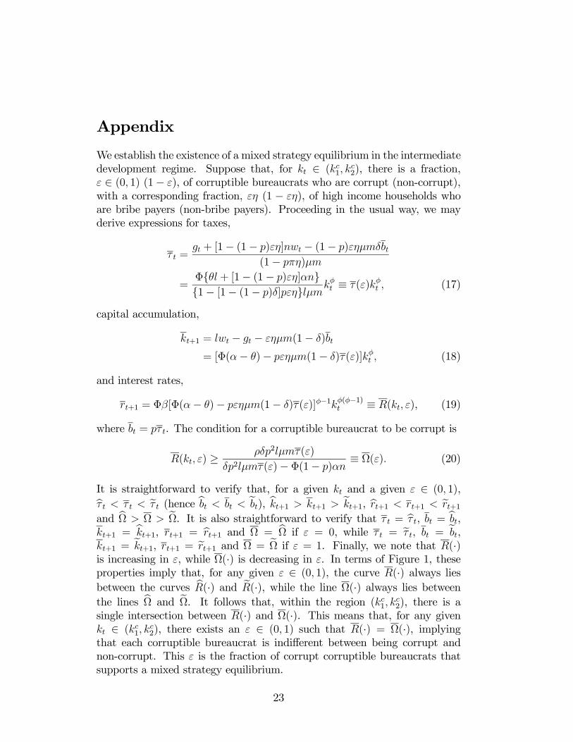
Appendix

We establish the existence of a mixed strategy equilibrium in the intermediatedevelopment regime. Suppose that, for kt ∈ (kc1, kc2), there is a fraction,ε ∈ (0, 1) (1− ε), of corruptible bureaucrats who are corrupt (non-corrupt),with a corresponding fraction, εη (1 − εη), of high income households whoare bribe payers (non-bribe payers). Proceeding in the usual way, we mayderive expressions for taxes,

τ t =gt + [1− (1− p)εη]nwt − (1− p)εηµmδbt

(1− pπη)µm

=Φθl + [1− (1− p)εη]αn1− [1− (1− p)δ]pεηlµmkφt ≡ τ(ε)kφt , (17)

capital accumulation,

kt+1 = lwt − gt − εηµm(1− δ)bt

= [Φ(α− θ)− pεηµm(1− δ)τ(ε)]kφt , (18)

and interest rates,

rt+1 = Φβ[Φ(α− θ)− pεηµm(1− δ)τ(ε)]φ−1kφ(φ−1)t ≡ R(kt, ε), (19)

where bt = pτ t. The condition for a corruptible bureaucrat to be corrupt is

R(kt, ε) ≥ ρδp2lµmτ(ε)

δp2lµmτ(ε)− Φ(1− p)αn≡ Ω(ε). (20)

It is straightforward to verify that, for a given kt and a given ε ∈ (0, 1),bτ t < τ t < eτ t (hence bbt < bt < ebt), bkt+1 > kt+1 > ekt+1, brt+1 < rt+1 < ert+1and bΩ > Ω > eΩ. It is also straightforward to verify that τ t = bτ t, bt = bbt,kt+1 = bkt+1, rt+1 = brt+1 and Ω = bΩ if ε = 0, while τ t = eτ t, bt = ebt,kt+1 = ekt+1, rt+1 = ert+1 and Ω = eΩ if ε = 1. Finally, we note that R(·)is increasing in ε, while Ω(·) is decreasing in ε. In terms of Figure 1, theseproperties imply that, for any given ε ∈ (0, 1), the curve R(·) always liesbetween the curves bR(·) and eR(·), while the line Ω(·) always lies betweenthe lines bΩ and eΩ. It follows that, within the region (kc1, kc2), there is asingle intersection between R(·) and Ω(·). This means that, for any givenkt ∈ (kc1, kc2), there exists an ε ∈ (0, 1) such that R(·) = Ω(·), implyingthat each corruptible bureaucrat is indifferent between being corrupt andnon-corrupt. This ε is the fraction of corrupt corruptible bureaucrats thatsupports a mixed strategy equilibrium.

23

References

[1] Acemoglou, D. and T. Verdier, 1998. Property rights, corruption and theallocation of talent: a general equilibrium approach. Economic Journal,108, 1381-1403.

[2] Acemoglou, D. and T. Verdier, 2000. The choice between market failuresand corruption. American Economic Review, 90, 194-211.

[3] Ades, A. and R. Di Tella, 1997. The new economics of corruption: asurvey and some new results. Political Studies, 45 (Special Issue), 496-515.

[4] Ades, A. and R. Di Tella, 1999. Rents, competition and corruption.American Economic Review, 89, 982-993.

[5] Andvig, J.C. and K.O. Moene, 1990. How corruption may corrupt. Jour-nal of Economic Behaviour and Organisations, 13, 63-76.

[6] Banerjee, A.V., 1997. A theory of misgovernance. Quarterly Journal ofEconomics, 112, 1289-1332.

[7] Bardhan, P., 1997. Corruption and development: a review of issues.Journal of Economic Literature, 35, 1320-1346.

[8] Bardhan, P., 2000. Corruption: a review. Journal of Economic Surveys,15, 71-116.

[9] Barro, R.J., 1990. Government spending in a simple model of endoge-nous growth. Journal of Political Economy, 98, S103-S125.

[10] Basu, S. and D.D. Li, 1998. Corruption in transition. University of Michi-gan Business School Working Paper No.161.

[11] Beck, P.J. and M.W. Maher, 1986. A comparison of bribery and biddingin thin markets. Economics Letters, 20, 1-5.

[12] Besley, T. and J. McLaren, 1993. Taxes and bribery: the role of wageincentives. Economic Journal, 119-141.

[13] Cadot, O., 1987. Corruption as a gamble. Journal of Public Economics,33, 223-244.

[14] Carillo, J.D., 2000. Corruption in hierarchies. Annales d’Economie et deStatistique, 10, 37-61.

24

[15] Ehrlich, I. and F.T. Lui, 1999. Bureaucratic corruption and endogenouseconomic growth. Journal of Political Economy, 107, 270-293.

[16] Gould, D.J. and J.A. Amaro-Reyes, 1983. The effects of corruption onadministrative performance. World Bank StaffWorking Paper No.580.

[17] Huntington, S.P., 1968. Political Order in Changing Societies. Yale Uni-versity Press, New Haven.

[18] Jain, A.K. (ed.), 1998. The Economics of Corruption. Kluwer AcademicPublishers, Massachusettes.

[19] Kauffman, D. and S.-J. Wei, 2000. Does “grease money” speed up thewheels of commerce? IMF Working Paper No.WP/00/64.

[20] Klitgaard, R., 1988. Controlling Corruption. University of CaliforniaPress, Berkeley.

[21] Klitgaard, R., 1990. Tropical Gangsters. Basic Books, New York.

[22] Klitgaard, R. 1991. Adjusting to reality: beyond state versus market ineconomic development. ICS Press and International Centre for EconomicGrowth, San Francisco.

[23] Leff, N.H., 1964. Economic development through bureaucratic corrup-tion. In A.K. Jain (ed.), The Economics of Corruption, Kluwer Acad-emic Publishers, Massachusettes.

[24] Leys, C., 1970. What is the problem about corruption? In A.J. Heiden-heimer (ed.), Political Corruption: Readings in Comparative Analysis,Holt Reinehart, New York.

[25] Lien, D.H.D., 1986. A note on competitive bribery games. EconomicsLetters, 22, 337-341.

[26] Lui, F., 1985. An equilibrium queuing model of corruption. Journal ofPolitical Economy, 93, 760-781.

[27] Mauro, P., 1995. Corruption and growth. Quarterly Journal of Eco-nomics, 110, 681-712.

[28] Mauro, P., 1997. The effects of corruption on growth, invsetment andgovernment expenditure: a cross-country analysis. In K.A. Elliott (ed.),Corruption and the Global Economy, Institute for International Eco-nomics, Washington D.C.

25

[29] Mookherjee, D. and I.P.L. Png, 1995. Corruptible law enforcers: howshould they be compensated? Economic Journal, 105, 145-159.

[30] Rose-Ackerman, S., 1975. The economics of corruption. Journal of Pub-lic Economics, 4, 187-203.

[31] Rose-Ackerman, S., 1978. Corruption: A Study in Political Economy.Academic Press.

[32] Rose-Ackerman, S., 1996. Democracy and the “grand” corruption. In-ternational Social Science Journal, 158, 365-380.

[33] Rose-Ackerman, S., 1998. Corruption and development. Annual WorldBank Conference on Development Economics 1997, 35-57.

[34] Rose-Ackerman, S., 1999. Corruption and Government: Causes, Con-sequences and Reform. Cambridge University Press, Cambridge.

[35] Sah, R.K., 1991. Social osmosis and patterns of crime. Journal of Polit-ical Economy, 99, 1272-1295.

[36] Sarte, P.-D., 2000. Informality and rent-seeking bureaucracies in a modelof long-run growth. Journal of Monetary Economics, 46, 173-197.

[37] Shleifer, A. and R. Vishny, 1993. Corruption. Quarterly Journal of Eco-nomics, 108, 599-617.

[38] Tanzi, V. and H. Davoodi, 1997. Corruption, public investment andgrowth. IMF Working Paper No.WP/97/139.

[39] Tirole, J., 1996. A theory of collective reputation (with applications tothe persistence of corruption and to firm quality). Review of EconomicStudies, 63, 1-22.

[40] Treisman, D., 2000. The causes of corruption: a cross-national study.Journal of Public Economics, 76, 399-457.

[41] United Nations, 1989. Corruption in Government. United Nations, NewYork.

[42] Wade, R. 1985. The market for public office: why the Indian state is notbetter at development. World Development, 13, 467-497.

26

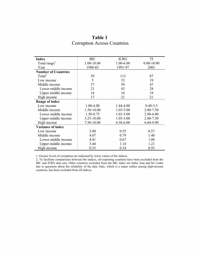
Table 1 Corruption Across Countries

Index BIC ICRG TI Total range1 1.00-10.00 1.00-6.00 0.00-10.00 Year 1980-83 1991-97 2001 Number of Countries Total2 59 113 87 Low income 5 33 19 Middle income 37 59 47 Lower middle income 21 43 28 Upper middle income 16 16 19 High income 17 21 21 Range of index Low income 1.00-4.00 1.44-4.00 0.40-3.5 Middle income 1.50-10.00 1.03-5.00 2.00-7.50 Lower middle income 1.50-8.75 1.03-5.00 2.00-6.00 Upper middle income 3.25-10.00 1.05-5.00 2.80-7.50 High income 7.50-10.00 4.38-6.00 6.60-9.90 Variance of index Low income 2.00 0.55 0.57 Middle income 4.07 0.79 1.40 Lower middle income 4.41 0.67 1.08 Upper middle income 3.44 1.14 1.21 High income 0.33 0.34 0.93

1. Greater levels of corruption are indicated by lower values of the indices. 2. To facilitate comparisons between the indices, oil-exporting countries have been excluded from the BIC and ICRG data sets. Other countries excluded from the BIC index are India, Iraq and Sri Lanka due to questions about the reliability of the data. Italy, which is a major outlier among high-income countries, has been excluded from all indices.

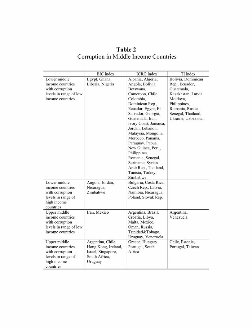
Table 2

Corruption in Middle Income Countries

BIC index ICRG index TI index Lower middle income countries with corruption levels in range of low income countries

Egypt, Ghana, Liberia, Nigeria

Albania, Algeria, Angola, Bolivia, Botswana, Cameroon, Chile, Colombia, Dominican Rep., Ecuador, Egypt, El Salvador, Georgia, Guatemala, Iran, Ivory Coast, Jamaica, Jordan, Lebanon, Malaysia, Mongolia, Morocco, Panama, Paraguay, Papua New Guinea, Peru, Philippines, Romania, Senegal, Suriname, Syrian Arab Rep., Thailand, Tunisia, Turkey, Zimbabwe

Bolivia, Dominican Rep., Ecuador, Guatemala, Kazakhstan, Latvia, Moldova, Philippines, Romania, Russia, Senegal, Thailand, Ukraine, Uzbekistan

Lower middle income countries with corruption levels in range of high income countries

Angola, Jordan, Nicaragua, Zimbabwe

Bulgaria, Costa Rica, Czech Rep., Latvia, Namibia, Nicaragua, Poland, Slovak Rep.

Upper middle income countries with corruption levels in range of low income countries

Iran, Mexico Argentina, Brazil, Croatia, Libya, Malta, Mexico, Oman, Russia, Trinidad&Tobago, Uruguay, Venezuela

Argentina, Venezuela

Upper middle income countries with corruption levels in range of high income countries

Argentina, Chile, Hong Kong, Ireland, Israel, Singapore, South Africa, Uruguay

Greece, Hungary, Portugal, South Africa

Chile, Estonia, Portugal, Taiwan

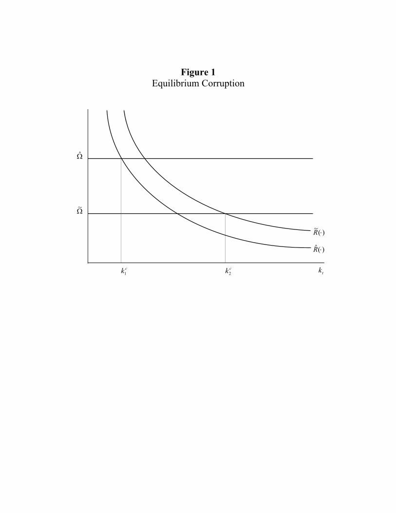
Figure 1 Equilibrium Corruption

)(ˆ ⋅R

)(~ ⋅R

ck1ck2 tk

Ω

Ω~

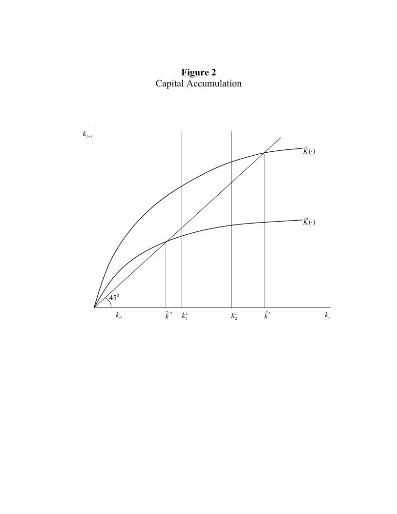
Figure 2 Capital Accumulation

ck1*~k *k

450

ck2 tk

1+tk

)(~ ⋅K

)(ˆ ⋅K

0k