Embed Size (px)
Citation preview

Research on Logic and Computation inHypothesis Finding
Yoshitaka Yamamoto
DOCTOR OF PHILOSOPHY
Department of Informatics,
School of Multidisciplinary Sciences
The Graduate University for Advanced Studies
2010
Contents
1 Introduction 1
1.1 Background . . . . . . . . . . . . . . . . . . . . . . . . . . . . 1
1.1.1 Abduction and Induction . . . . . . . . . . . . . . . . . 2
1.1.2 Inductive Logic Programming . . . . . . . . . . . . . . 8
1.1.3 Applicability in Life Sciences . . . . . . . . . . . . . . . 14
1.2 Motivation . . . . . . . . . . . . . . . . . . . . . . . . . . . . . 18
1.3 Contribution . . . . . . . . . . . . . . . . . . . . . . . . . . . . 21
1.4 Overview . . . . . . . . . . . . . . . . . . . . . . . . . . . . . . 22
1.5 Publications . . . . . . . . . . . . . . . . . . . . . . . . . . . . 23
2 Preliminaries 25
2.1 First-Order Logic . . . . . . . . . . . . . . . . . . . . . . . . . 25
2.2 Normal Forms and Herbrand’s Theorem . . . . . . . . . . . . 30
2.3 Consequence Finding . . . . . . . . . . . . . . . . . . . . . . . 33
2.4 Dualization . . . . . . . . . . . . . . . . . . . . . . . . . . . . 38
3 Inverse Entailment and CF-induction 45
3.1 Hypothesis Finding in Inverse Entailment . . . . . . . . . . . . 45
3.2 CF-induction . . . . . . . . . . . . . . . . . . . . . . . . . . . 48
4 Theory Completion using CF-induction: Case Study 63
4.1 Introduction . . . . . . . . . . . . . . . . . . . . . . . . . . . . 63
4.2 Logical Modeling of Metabolic Flux Dynamics . . . . . . . . . 66
4.2.1 Metabolic Pathways . . . . . . . . . . . . . . . . . . . 66
4.2.2 Regulation of Enzymatic Activities . . . . . . . . . . . 69
i

4.3 Experiments . . . . . . . . . . . . . . . . . . . . . . . . . . . . 72
4.3.1 Simple Pathway . . . . . . . . . . . . . . . . . . . . . . 72
4.3.2 Metabolic Pathway of Pyruvate . . . . . . . . . . . . . 76
4.4 Related Work . . . . . . . . . . . . . . . . . . . . . . . . . . . 79
4.5 Summary . . . . . . . . . . . . . . . . . . . . . . . . . . . . . 82
5 From Inverse Entailment to Inverse Subsumption 83
5.1 Introduction . . . . . . . . . . . . . . . . . . . . . . . . . . . . 83
5.2 Inverse Subsumption with Residue Complements . . . . . . . . 85
5.3 Inverse Subsumption with Minimal Complements . . . . . . . 88
5.3.1 Fixed-Point Theorem on Minimal Complements . . . . 88
5.3.2 Inverting Deductive Operations with Tautologies . . . 91
5.3.3 Deriving Hypotheses with Induction Fields . . . . . . . 96
5.4 Discussion . . . . . . . . . . . . . . . . . . . . . . . . . . . . . 98
5.5 Summary . . . . . . . . . . . . . . . . . . . . . . . . . . . . . 106
6 Logical Reconstruction in CF-induction 108
6.1 Introduction . . . . . . . . . . . . . . . . . . . . . . . . . . . . 108
6.2 CF-induction with Deductive Operations . . . . . . . . . . . . 110
6.2.1 Logical Relation Between Bridge Theories
and Ground Hypotheses . . . . . . . . . . . . . . . . . 112
6.2.2 Deriving Non-Ground Hypotheses . . . . . . . . . . . . 115
6.2.3 Related Work . . . . . . . . . . . . . . . . . . . . . . . 118
6.3 CF-induction with Inverse Subsumption . . . . . . . . . . . . 119
6.3.1 Logical Relation between Production Fields
and Induction Fields . . . . . . . . . . . . . . . . . . . 119
6.3.2 Deriving Hypotheses with Induction Fields . . . . . . . 121
6.4 Comparison . . . . . . . . . . . . . . . . . . . . . . . . . . . . 122
6.5 Summary . . . . . . . . . . . . . . . . . . . . . . . . . . . . . 127
7 Conclusions and Future Work 128
7.1 Summary . . . . . . . . . . . . . . . . . . . . . . . . . . . . . 128
7.2 Future Work . . . . . . . . . . . . . . . . . . . . . . . . . . . . 130
ii

Bibliography 142
iii

List of Figures
1.1 Integration of Abduction with Induction . . . . . . . . . . . . 4
1.2 Hypotheses in Each Framework of Induction . . . . . . . . . . 7
1.3 Michalski’s Train Example . . . . . . . . . . . . . . . . . . . . 12
1.4 Protein Folding Prediction as Classification Problem . . . . . 14
1.5 Possible Gene Regulatory Networks . . . . . . . . . . . . . . . 16
1.6 Mutant Data and Generated Gene Network . . . . . . . . . . 16
1.7 Knowledge Discovery in Systems Biology . . . . . . . . . . . . 18
2.1 Tableau in SOLAR . . . . . . . . . . . . . . . . . . . . . . . . 38
3.1 Characteristics in IE-based Methods . . . . . . . . . . . . . . 48
4.1 Dynamics Emerged in The Growth of Yeast . . . . . . . . . . 67
4.2 Transition of Master Reactions . . . . . . . . . . . . . . . . . 67
4.3 System of Mass Balance . . . . . . . . . . . . . . . . . . . . . 68
4.4 First Biological Inference in Metabolic Pathways . . . . . . . . 70
4.5 Second Biological Inference in Metabolic Pathways . . . . . . 70
4.6 First Hypothesis H1 . . . . . . . . . . . . . . . . . . . . . . . 73
4.7 Second Hypothesis H2 . . . . . . . . . . . . . . . . . . . . . . 73
4.8 Metabolic Pathway of Pyruvate . . . . . . . . . . . . . . . . . 77
4.9 Third Hypothesis H3 . . . . . . . . . . . . . . . . . . . . . . . 78
4.10 Forth Hypothesis H4 . . . . . . . . . . . . . . . . . . . . . . . 78
4.11 Integrating Abduction and Induction for Finding Hypotheses . 81
5.1 Hypothesis Finding Based on Inverse Entailment . . . . . . . . 84
5.2 Hypothesis Finding Based on Inverse Subsumption . . . . . . 85
5.3 Deductive Operations in Example 5.1 . . . . . . . . . . . . . . 93
iv
5.4 Deductive Operations in Example 5.5 . . . . . . . . . . . . . . 94
5.5 Example of Inverse Resolution . . . . . . . . . . . . . . . . . . 100
5.6 Inverting Resolution by Adding Tautologies . . . . . . . . . . 101
5.7 Setting for V-operator . . . . . . . . . . . . . . . . . . . . . . 102
5.8 Possible Hypotheses Obtained by Inverse Entailment . . . . . 106
6.1 Hypothesis Finding in CF-induction . . . . . . . . . . . . . . . 108
6.2 Search Strategies in Two Approaches . . . . . . . . . . . . . . 123
v
Acknowledgements
I am very grateful to my supervisor, Pr. Katsumi Inoue. It was still in my
undergraduate course at his laboratory when I involved in the research topic
on hypothesis finding. Since this time, I have continued to study this topic.
I could not complete this thesis without his generous support and patience
during my time as an undergraduate, graduate and PhD student. I am very
grateful to Pr. Ken Sato, Pr. Makoto Tatsuta, Pr. Akihiro Yamamoto and
Pr. Taisuke Sato for their inspiration and fruitful comments on this work.
Their advice on the research topics encouraged me to write the thesis. I
would also like to present my sincere thanks to Pr. Koji Iwanuma for his
constant and kind support.
Motivation for this thesis also emanated from precious meeting with my
colleagues in National Institute of Informatics (NII). Pr. Andrei Doncescu
impressed me with the interests in systems biology. I benefited from the
broad experience to study on Systems Biology at the laboratory of Pr. Gerald
Goma in Toulouse. Another inspiring stay was my visit to Dr. Oliver Ray in
Bristol. Discussions with him greatly stimulated me and gave some insights
on the research.
I would like to thank Pr. Hidetomo Nabeshima for his kind advice on
SOLAR and implementation of CF-induction, Pr. Yoshitaka Kameya for his
beneficial comments on relational learning, and Pr. Stephen Muggleton and
Pr. Gilles Richard for their constructive discussions in NII. I would also like
to thank the anonymous refers of several conferences and workshops for their
feedback on parts of this thesis.
I gladly acknowledge the financial support of NII as well as both Japan
Science and Technology Agency (JST) and Centre National de la Recherche
vi

Scientifique (CNRS, France) under the 2007-2009 Strategic Japanese-French
Cooperative Program ”Knowledge-based Discovery in Systems Biology”, and
also 2008-2011 JSPS Grant-in-Aid Scientific Research (A) (No. 20240016). I
owe my thanks to Takehide Soh, the secretaries at our laboratory and the
staffs at the Graduate University for Advanced Studies for their kind help
and constant encouragement.
Last, I wish to thank my parents Takemi and Shizuko and my family
Ayuka and our kid, Kousei for their understanding and continuous supports
that have made me overcome any difficulties in my life.
vii

Abstract
The thesis studies the logical mechanism and its computational proce-
dures in hypothesis finding. Given a background theory and an observation
that is not logically derived by the prior theory, we try to find a hypothesis
that explains the observation with respect to the background theory. The
hypothesis may contradict with a newly observed fact. That is why the logic
in hypothesis finding is often regarded as ampliative inference.
In first-order logic, the principle of inverse entailment (IE) has been ac-
tively used to find hypotheses. Previously, many IE-based hypothesis finding
systems have been proposed, and several of them are now being applied to
practical problems in life sciences concerned with the study of living or-
ganisms, like biology. However, these state-of-the-art systems have some
fundamental limitation on hypothesis finding: They make the search space
restricted due to computational efficiency. For the sake of incompleteness in
hypothesis finding, there is an inherent possibility that they may fail to find
such sufficient hypotheses that are worth examining.
The thesis first provides such a practical problem, where those incomplete
procedures cannot work well. In contrast, this motivating problem is solved
by CF-induction, which is an IE-based procedure that enables us to find
every hypothesis. On the other hand, complete procedures like CF-induction
have to deal with a huge search space, and thus, are usually achieved by
consisting of many non-deterministic procedures.
The thesis next shows an alternative approach for finding hypotheses,
which is based on the inverse relation of subsumption, instead of entailment.
The proposed approach is used to simplify the IE-based procedures by reduc-
ing their non-determinisms without losing completeness in hypothesis finding.
Together with this result, we logically reconstruct the current procedure of
CF-induction into a more simplified one, while it ensures the completeness.
Through the thesis, we will see underlying nature and insights to overcome
limitations in the current IE-based hypothesis finding procedures.

Chapter 1
Introduction
1.1 Background
We are used to hypothesize in various aspects of daily life. When infant
children are crying, their mothers would give some milk to the infants. That
is because mothers consciously or not hypothesize that infants want some
milk when they cry. Hypothesizing also plays an important role in business.
When quality-engineers face some claim to a product from the market, they
would examine whether or not the other products in the same lot have the
same defect. That is because they hypothesize that if some product includes
a defect, the others in the same lot can also include the same defect.
According to a dictionary, the word “hypothesis” means a proposition
made as a basis for reasoning, without the assumption of its truth. In other
words, generated hypotheses are not necessarily always in the right. Indeed,
crying children may want to change diapers and products with some defect
may be occurred singly. That is why the logic in hypothesizing is viewed as
ampliative inference: abduction and induction, which are epistemologically
distinguished with deductive inference.
Research topics on inference-based hypothesis finding have been actively
studied in the community of inductive logic programming (ILP). Historically,
ILP has been first defined as the intersection of machine learning and logic
programming to deal with induction in first-order logic [43, 48, 36]. Com-
pared with the other machine learning techniques, ILP works on both tasks
1
of classification and theory completion in complex-structured data.
Oceans of data are now being generated in great volumes and in diverse
formats. In life sciences, biochemical data is also rapidly produced from
emerging high throughput techniques, whereas the whole life-systems, such
as signal transduction, gene regulation and metabolism, are still incompletely
clarified. For this situation, ILP techniques are recently being applied in life
sciences to find hypotheses that can complete the prior life-systems. The
huge and diverse biochemical data can be lumped with richer knowledge
representation formalisms in first-order logic. Thus, unlike the other machine
learning techniques, ILP has applicability to discovering causal relations and
missing facts that are lacked in the biochemical knowledge.
In this section, we first review abduction and induction by explaining
their tasks, similarities and differences as well as introducing several kinds of
inductive tasks. Next, we review inductive logic programming by describing
the task and advantages as well as its history in brief. Lastly, we consider
an inherent possibility to apply ILP techniques in life sciences by reviewing
several past application examples.
1.1.1 Abduction and Induction
Both abduction and induction are ampliative inference to seek a hypothe-
sis that accounts for given observations or examples. Generated hypotheses
provide us more information by adding them to the prior background knowl-
edge. On the other hand, it may be falsified when new knowledge is obtained.
According to the philosopher C. S. Peirce [53, 24], whereas induction infers
similarities or regularities confirmed in the observations, abduction infers
causalities that are different from what we directly observe. For instance,
from the positions of planets in the space, inferring that the planets move
in ellipses with the sun is an inductive task. Because this task is related to
finding a similarity hidden in the orbits of planets. In contrast, from the ob-
servation that an apple drops on the ground, inferring the existence of gravity
is an abductive task. That is because though the concept of gravity explains
the observation, we cannot explicitly sense the existence of gravity. We note
2

that the word “abduction” is used to mention the property taking subjects
away illegally in general. Indeed, we often see this word in articles on the
North Korea abductions of Japanese. Similarly, abduction as the inference is
also used to bring us unexpected inspirations with respect to observations.
As the discovery of universal gravitation, discerning hypotheses often have
loaded to paradigm shifts in science. Not only in science, but also in business
or everyday life, we use induction and abduction especially for generating
theories. Let us give a toy example (1): Suppose that when we walk around
a university in autumn, we observe that a tree on the east side begins to turn
color faster than others. From the observation, we may infer the abductive
hypothesis that the sunlight causes the autumn color in the tree. That is
because the sunlight tends to get into trees on the east side more brightly than
others on the west. By generalizing the abductive hypothesis, we may obtain
the inductive hypothesis: if an arbitrary tree is much sun-exposed, then it
turns color faster than others. This inductive hypothesis can be verified by
checking whether or not it is applicable to another tree. If the verification
results in rejection of the current hypothesis, we need to refine it and verify
once again the modified one. Otherwise, we can keep the current hypothesis
as it is. In this way, we generate a concrete theory using abduction and
induction in the cycle of hypothesis formation and verification.
From an epistemological point of view, abduction and induction are clearly
two different processes. On the one hand, induction refers to inductive gen-
eralization: It is used to find general laws that account for given observations
possibly with the background theory. On the other hand, abduction is used
to infer an explanation for some specific observed situations or properties.
However, in a logical standpoint, they are not necessarily distinguished with
each other, because induction can often induce explanations for the obser-
vations. Recall the example [22] where we know Tweety is a bird and we
suddenly observe that he is able to fly. Then, we may infer that every bird
can fly. This hypothesis is an inductive generalization, and simultaneously,
can be regarded as an explanation for the observation.
Lachiche [33] pointed out this identification in abduction and induction,
and especially called the “explanation-based” induction as explanatory in-
3

duction. Given a background theory B and observations E, the task of
explanatory induction is to find a hypothesis H such that
B ∧ H |= E, (1.1)
B ∧ H is consistent, (1.2)
where B∧H |= E denotes the entailment relation1 that if B and H are true,
then E is also true in brief.
Formulas (1.1) and (1.2) can be adopted in the logical formalization of
abduction. That is because hypotheses generated by abduction are explana-
tions of observations that satisfy two formulas. Hence, explanatory induc-
tion provides an integrated framework of induction with abduction. In other
word, explanatory induction can find both inductive and abductive hypothe-
ses. The above example (1), described in Figure 1.1, is such a case that
abduction and induction are necessary to generate the target hypothesis.
B: locate(X, east) → sunlight(X)
E: locate(tree(a), east) → autumn color(tree(a))
(abduction) sunlight(tree(a), east) → autumn color(tree(a))
(induction) sunlight(tree(X), east) → autumn color(tree(X))
Figure 1.1: Integration of Abduction with Induction
Along with explanatory induction, several different formalizations of in-
duction has been proposed in the literature [22, 21, 33, 27, 66] such as
Descriptive induction, Circumscriptive induction and Brave induction. In
explanatory induction, it is often difficult to infer regularities confirmed in
observations [22]. For instance, suppose that we have two plastic bottles such
that the one is hot and the other is cold, and we suddenly notice that the
former has a red cap whereas the latter has a white cap. Then, we may infer
that plastic bottles with a red (resp. white) cap are hot (resp. cold). This
is an inductive hypothesis that shows a general relation between cap color
1Please see Chapter 2 for the precise definition.
4

and temperature in plastic bottles. However, explanatory induction cannot
generate this hypothesis. Instead, it infers an alternative hypothesis that
hot (resp. cold) bottles have a red (resp. hot) cap. We can represent this
example with the logical formalization as follows:
B : hot(b1) ∧ cold(b2).
E : cap(b1, red) ∧ cap(b2, white).
H1 : (cap(X, red) → hot(X)) ∧ (cap(X,white) → cold(X)).
H2 : (hot(X) → cap(X, red)) ∧ (cold(X) → cap(X,white)).
Though H1 is a considerable hypothesis generated by induction, it cannot
explain E with respect to B. Accordingly, H1 cannot be obtained in the
context of explanatory induction. Descriptive induction [22, 21, 33] has been
proposed to come up with this limitation in explanatory induction. A hypoth-
esis H in descriptive induction is usually defined with so-called completion
technique, and satisfies the following condition:
Comp(B ∧ E) |= H. (1.3)
where Comp(B ∧ E) denotes the predicate completion relative to all predi-
cates in B∧E [8]. In the above example, Comp(B∧E) is obtained by adding
the following theories to B ∧ E:
(hot(X) → X = b1) ∧ (cold(X) → X = b2).
(cap(X, red) → X = b1) ∧ (cap(X,white) → X = b2).
Roughly speaking, these formulas complete the extensions of each predicate
hot, cold and cap using individuals that appear in B∧E. Since Comp(B∧E)
derives H1 and H2, both are hypotheses of descriptive induction, whereas only
H1 can be derived by explanatory induction.
If we should accept the task of induction as completion of individuals that
Lachiche [33] pointed out, descriptive induction based on Clark’s predicate
completion is an alternative but different kind of inductive inference from
explanatory induction. Compared with descriptive induction, explanatory
induction finds classifications rather than regularities or similarities hidden
5

in observations. In fact, the hypothesis H2 obtained by explanatory induction
classifies each plastic bottle into two classes (that is, the one with a red cap
and another with a white cap) according to its temperature. Note that every
hypothesis obtained by explanatory induction is not necessarily solved by
descriptive induction as follows:
B : plus(X, 0, X).
E : plus(X, s(0), s(X)).
H : plus(X,Y, Z) → plus(X, s(Y ), s(Z)).
The predicate plus(X,Y, Z) means that the sum of X and Y is equal to
Z. s(X) denotes the successor function of X that satisfies s0(X) = X and
sn(X) = s(sn−1(X)). Since H logically explains E with respect to B, H is
a hypothesis in explanatory induction. On the other hand, this hypothesis
cannot be obtained by descriptive induction. Indeed, the completion theory
Comp(B ∧ E) does not derive H, which is obtained by adding the following
theory to B ∧ E:
plus(X,Y, Z) → (Y = 0 ∧ Z = X) ∨ (Y = s(0) ∧ Z = s(X)).
In the case of Y = 0 and Z = X, plus(X, s(Y ), s(Z)) holds since this becomes
equivalent to E = plus(X, s(0), s(X)). However, in the other case of Y =
s(0) and Z = s(X), plus(X, s(Y ), s(Z)) does not hold since Comp(B ∧ E)
never state whether or not plus(X, s2(0), s2(X)) is true. We may notice
that H is a missing definition of addition. In other word, H completes the
prior (incomplete) background theory. In this sense, explanatory induction
is suitable for inductive tasks such as theory completion [27].
There is an integrated framework of explanatory induction with descrip-
tive induction, called circumscriptive induction [27]. This overcomes induc-
tive leap that explanatory induction can pose. Let the background theory B
and the observation E as follows:
B : bird(Tweety) ∧ bird(Oliver).
E : flies(Tweety).
6
Explanatory induction then infers the hypothesis bird(X) → flies(X). This
hypothesis logically explains not only the observation flies(Tweety), but
also flies(Oliver) that is regarded as an inductive leaf. Because we cannot
state that Oliver also flies like Tweety by the prior knowledge. In contrast,
circumscriptive induction infers an alternative hypothesis H based on the
notion of circumscription [39] as follows:
bird(X) ∧ X 6= Oliver → flies(X).
Since H logically explains E with B and also is derived from Comp(B ∧E),
H is a hypothesis in both explanatory and descriptive induction.
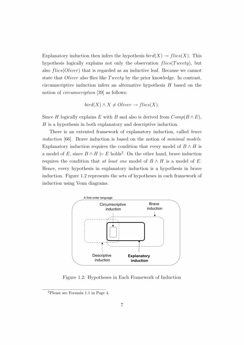
There is an extented framework of explanatory induction, called brave
induction [66]. Brave induction is based on the notion of minimal models.
Explanatory induction requires the condition that every model of B ∧ H is
a model of E, since B ∧ H |= E holds2. On the other hand, brave induction
requires the condition that at least one model of B ∧ H is a model of E.
Hence, every hypothesis in explanatory induction is a hypothesis in brave
induction. Figure 1.2 represents the sets of hypotheses in each framework of
induction using Venn diagrams.
Descriptive induction
Explanatory induction
Circumscriptive induction
Brave induction
A first-order language
Figure 1.2: Hypotheses in Each Framework of Induction
2Please see Formula 1.1 in Page 4.
7

Induction played a central role at the beginning of machine learning field,
and it has been evolved into powerful systems for solving classification prob-
lems and recently for theorem completion in a relative young branch of ma-
chine learning: ILP. We next briefly describes the inter-related histories of
machine learning and ILP.
1.1.2 Inductive Logic Programming
Within Machine Learning, the research field of ILP is characterized as one
of the paradigms, called inductive learning. Unlike the other paradigms
such as the analytic paradigms, the connectionist paradigm and the genetic
paradigm, its aim is to induce a general concept description from a sequence
of instances of the concept and known counterexamples of the concept [6].
In the historical perspective3, the inductive learning has been developed
interacting with development of deduction as its counterpart. It seems likely
to be natural to go back two underlying theorems given by Godel [18] around
early 1930’s. Godel demonstrated that a small collection of sound rules of
inference was complete for deriving all consequeces, and after a year that
he proved this completeness result, in 1931, he proved the more famous
incompleteness theorem that Peano’s axiomisation of arithmetic, and any
first-order theory containing it, is either-contradictory or incomplete for de-
riving certain arithmetic statements. These theorems by far influences both
research fields of deduction and induction. The second incompleteness the-
orem involved many computer scientists like Turing [77] in noticing that in-
telligent machines require the capability of learning from examples. In turn,
the first complete theorem much later resulted as the fruitful discovery of
resolution principle given by Robinson [64], where a single rule of inference,
called resolution, is both sound and complete for proving statements within
this calculus. Based on his discovery, a simple question might arise through
visionary researchers: “If all the consequences can be derived from logical ax-
ioms by deduction, then where do the axioms come from?”. Indeed, around
the most same time as Robinson’s discovery, Banerji [4] tried to introduce
3Much of this subsection is adopted from [34, 43, 80]
8
the predicate logic formalization in inductive learning.
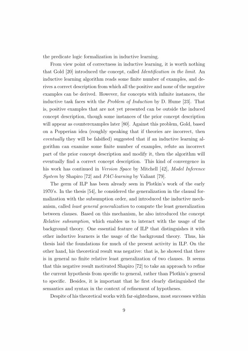
From view point of correctness in inductive learning, it is worth nothing
that Gold [20] introduced the concept, called Identification in the limit. An
inductive learning algorithm reads some finite number of examples, and de-
rives a correct description from which all the positive and none of the negative
examples can be derived. However, for concepts with infinite instances, the
inductive task faces with the Problem of Induction by D. Hume [23]. That
is, positive examples that are not yet presented can be outside the induced
concept description, though some instances of the prior concept description
will appear as counterexamples later [80]. Against this problem, Gold, based
on a Popperian idea (roughly speaking that if theories are incorrect, then
eventually they will be falsified) suggested that if an inductive learning al-
gorithm can examine some finite number of examples, refute an incorrect
part of the prior concept description and modify it, then the algorithm will
eventually find a correct concept description. This kind of convergence in
his work has continued in Version Space by Mitchell [42], Model Inference
System by Shapiro [72] and PAC-learning by Valiant [79].
The germ of ILP has been already seen in Plotkin’s work of the early
1970’s. In the thesis [54], he considered the generalization in the clausal for-
malization with the subsumption order, and introduced the inductive mech-
anism, called least general generalization to compute the least generalization
between clauses. Based on this mechanism, he also introduced the concept
Relative subsumption, which enables us to interact with the usage of the
background theory. One essential feature of ILP that distinguishes it with
other inductive learners is the usage of the background theory. Thus, his
thesis laid the foundations for much of the present activity in ILP. On the
other hand, his theoretical result was negative: that is, he showed that there
is in general no finite relative least generalization of two clauses. It seems
that this negative result motivated Shapiro [72] to take an approach to refine
the current hypothesis from specific to general, rather than Plotkin’s general
to specific. Besides, it is important that he first clearly distinguished the
semantics and syntax in the context of refinement of hypotheses.
Despite of his theoretical works with far-sightedness, most successes within
9

machine learning field have derived from systems which construct hypothe-
ses within the limits of propositional logic. For instance, MYCIN by Short-
liffe, Buchaman [73] and BMT based on Quinlan’s ID3 algorithm [57] were
efficiently applied as expert systems for specific domains such as medical
diagnosis. In 1980’s, several inductive systems within the predicate logic
formalization have been proposed for the sake of the limitations in propo-
sitional logic. Sammut and Banerji [67] introduced a system called MAR-
VIN which generalizes a single example at a time with reference to a set of
background clauses. In turn, Quinlan [58] described a system, called FOIL,
which performs a heuristic search from specific to general with the notion
of an information criterion related to entropy. Note that, whereas MARVIN
uses the background theory, FOIL does not distinguish the inputs into ex-
amples and the background theory. From this difference, MARVIN would
be characterized as one of the ancestors continuing in the present systems.
Indeed, Muggleton et al. showed that the generalization in MARVIN is a
specific case of inverting reolution processes, and described a system, called
GOLEM, which is based on a relative general generaltization [49]. In 1991, a
year before he described GOLEM, the first international conference on ILP
has held at Viana Do Castelo in Porto.
After the establishment of this conference, ILP has been evolved as the
research area including theory concerning induction (not only explanatory
induction, but also the other inductive frameworks that we showed above)
and abduction, implementation and experimental applications so far. In
summary, compared with the other inductive learning techniques, we list
three merits of ILP as follows:
• Rich representation formalisms: ILP uses the first-order predicate logic.
This feature enables to bring us beyond the restricted formalisms in
propositional logic. As a result, ILP can deal with highly-complex
structured data, which attribute-based algorithms like decision trees
cannot do.
• Usage of the background knowledge: ILP distinguishes the input for-
mulas into examples and the background knowledge if it is necessary.
10

In everyday life, we are used to utilize the background knowledge. In
this sense, it would be natural to use the background theory for finding
hypotheses.
• Integrated framework of abduction and induction: In the context of ex-
planatory induction, ILP can perform both abduction and induction.
For this feature, it can potentially find some missing general rules or
facts in the prior background theory. This becomes important espe-
cially in case that the background theory is assumed to be incomplete.
• Readability of the output theory: Unlike other inductive learning tech-
niques, such as Neural networks, Baysian networks and SVM, outputs
of ILP are represented as formulas that we can easily read and verify
them. For readability of the output theory, ILP can involve hypothesis
formation in scientific discovery by directly interacting with users.
We recall the Michalski’s train example [35]. This example would give us
an insight to see what kind of problems ILP sufficiently works on, compared
with other inductive learning algorithms.
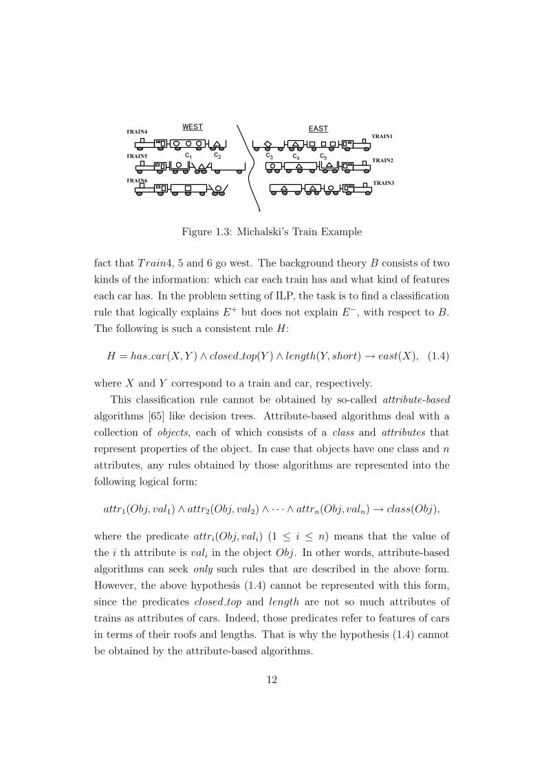
Michalski’s train example [35]: We observe two kinds of trains: One goes
west and the other goes east (See Figure 1.3). Every train contains several
cars each of which carries cargos and has its own shape. The task is to
discover a regulatory relation that decides the direction of each train. The
prior knowledge of each train and car is represented in first-order language.
For instance, Train1 and Car1 are as follows:
Train 1 : east(t1). has car(t1, c3). has car(t1, c4). has car(t1, c5).
Car 1 : closed top(c1). length(c1, long). has cargo(c1, circle).
Note that the predicate has car(t, c) means the train t contains the car c,
the predicate closed top(c) means the car c is closed at its top, the predicate
length(c, long) (resp. length(c, short)) means the length of the car c is long
(resp. short) and the predicate has cargo(c,X) means the car c has at least
one X-shaped cargo. The positive examples E+ correspond to the fact that
Train1, 2 and 3 go east. In contrast, we treat as the negative examples the
11
TRAIN1
TRAIN2
TRAIN3
TRAIN4
TRAIN5
TRAIN6
WEST EAST
c1 c2 c3 c4 c5
Figure 1.3: Michalski’s Train Example
fact that Train4, 5 and 6 go west. The background theory B consists of two
kinds of the information: which car each train has and what kind of features
each car has. In the problem setting of ILP, the task is to find a classification
rule that logically explains E+ but does not explain E−, with respect to B.
The following is such a consistent rule H:
H = has car(X,Y ) ∧ closed top(Y ) ∧ length(Y, short) → east(X), (1.4)
where X and Y correspond to a train and car, respectively.
This classification rule cannot be obtained by so-called attribute-based
algorithms [65] like decision trees. Attribute-based algorithms deal with a
collection of objects, each of which consists of a class and attributes that
represent properties of the object. In case that objects have one class and n
attributes, any rules obtained by those algorithms are represented into the
following logical form:
attr1(Obj, val1) ∧ attr2(Obj, val2) ∧ · · · ∧ attrn(Obj, valn) → class(Obj),
where the predicate attri(Obj, vali) (1 ≤ i ≤ n) means that the value of
the i th attribute is vali in the object Obj. In other words, attribute-based
algorithms can seek only such rules that are described in the above form.
However, the above hypothesis (1.4) cannot be represented with this form,
since the predicates closed top and length are not so much attributes of
trains as attributes of cars. Indeed, those predicates refer to features of cars
in terms of their roofs and lengths. That is why the hypothesis (1.4) cannot
be obtained by the attribute-based algorithms.
12

This example shows that ILP can find a classification rule between a
target class (i.e. Direction) and properties (i.e. roof and length) of an at-
tribute (i.e. car) in objects (i.e. trains). In this way, ILP focuses on not
only attributes but also those features using rich representation formalisms
in first-order logic. For this feature, ILP has been applied to classification
problems that deal with multiple hierarchic structures.
Along with classification, ILP is used for theory completion tasks.
Graph completion problem: Let us give such a toy example.
d
cb
a
①
②
③
④
Consider the left graph con-
sisting of four nodes a, b, c
and d, and two arcs a → c
and b → d. The left graph
describes the background the-
ory. Suppose that we newly
observe there is a path from
a to d. This cannot be ex-
plained by the background
theory. This means the prior graph is incomplete in the sense that the graph
has some missing arc. For this incomplete graph, ILP can find possible arcs
like c → d (1), a → b (2), c → b (3) or a → d (4) in the context of explana-
tory induction. It is not straightforward that the other machine learning
techniques such as decision trees, Neural networks and SVM perform this
kind of learning task, called theory completion.
As we described above, ILP is sufficient for the classification and theory
completion problems that deal with complex structured data. Based on this
feature, recently it has been growing interest to apply ILP techniques to
practical problems in life sciences. Its common motivation comes from the
perspective that ILP can find some unknown causal relations or missing facts
that are lacked in biochemical knowledge database. We next describe such
applicability in life sciences by introducing several practical problems where
ILP techniques were actually applied and successfully working.
13
1.1.3 Applicability in Life Sciences
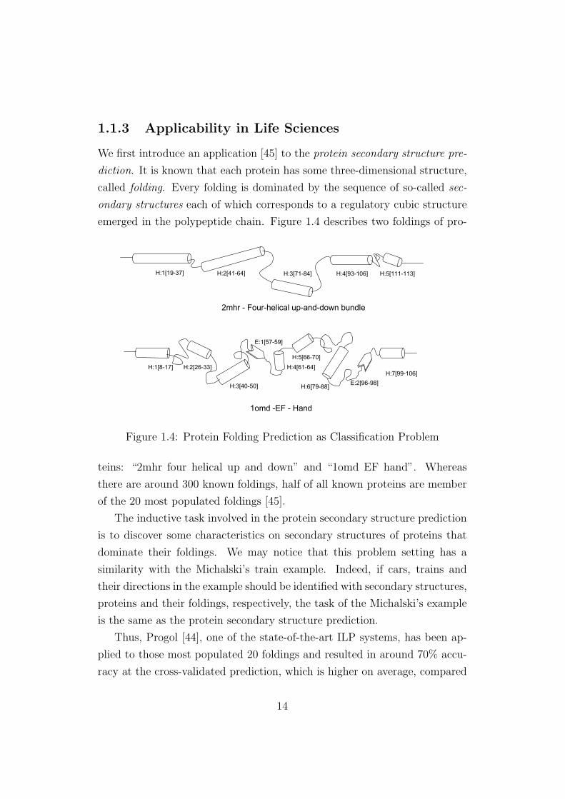
We first introduce an application [45] to the protein secondary structure pre-
diction. It is known that each protein has some three-dimensional structure,
called folding. Every folding is dominated by the sequence of so-called sec-
ondary structures each of which corresponds to a regulatory cubic structure
emerged in the polypeptide chain. Figure 1.4 describes two foldings of pro-
H:1[19-37] H:2[41-64] H:3[71-84] H:4[93-106] H:5[111-113]
2mhr - Four-helical up-and-down bundle
H:1[8-17] H:2[26-33]
H:3[40-50]
H:4[61-64]H:5[66-70]
1omd -EF - Hand
E:1[57-59]
H:6[79-88] E:2[96-98]H:7[99-106]
Figure 1.4: Protein Folding Prediction as Classification Problem
teins: “2mhr four helical up and down” and “1omd EF hand”. Whereas
there are around 300 known foldings, half of all known proteins are member
of the 20 most populated foldings [45].
The inductive task involved in the protein secondary structure prediction
is to discover some characteristics on secondary structures of proteins that
dominate their foldings. We may notice that this problem setting has a
similarity with the Michalski’s train example. Indeed, if cars, trains and
their directions in the example should be identified with secondary structures,
proteins and their foldings, respectively, the task of the Michalski’s example
is the same as the protein secondary structure prediction.
Thus, Progol [44], one of the state-of-the-art ILP systems, has been ap-
plied to those most populated 20 foldings and resulted in around 70% accu-
racy at the cross-validated prediction, which is higher on average, compared
14
with other machine learning techniques [45, 50]. For example, in the case
of “Four helical up and down bundle” in Figure 1.4, Progol generated the
following considerable hypothesis:
The protein P has this fold if it contains a long helix H1 at a position
between 1 and 3, and H1 is followed by a second helix H2.
In this problem, ILP was used as a classification tool in inductive learning.
As we explained before, ILP can be also used in a theory completion tool in
the context of explanatory induction.
B. Zupan et al. have developed so-called GenePath system to automati-
cally construct the genetic networks from mutant data [93, 94]. Their work
can be viewed as another application of ILP using the function of theory
completion. A gene regulatory network is usually described by a collection
of interactions between genes, which is involved in physiological behavior,
called phenotype, in a target life system. For understanding the influence of
a target gene on phenotype, geneticists make a mutant obtained by usually
knocking out the gene, and verify how phenotype emerges in the mutant.
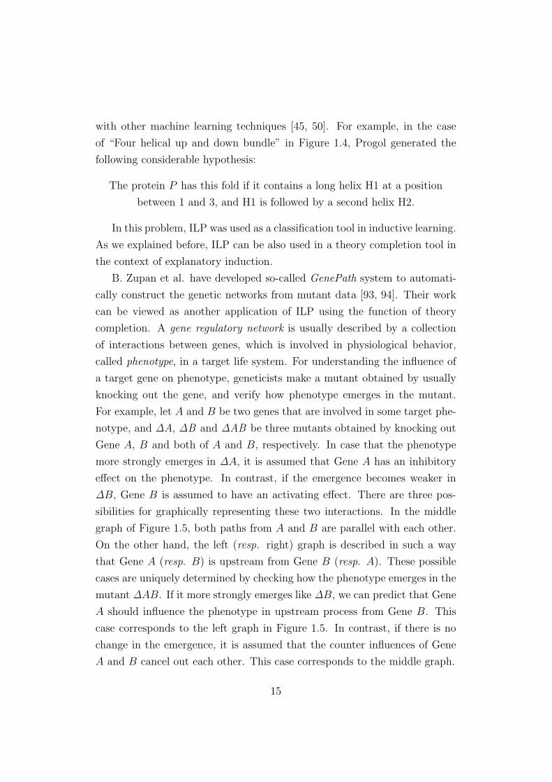
For example, let A and B be two genes that are involved in some target phe-
notype, and ∆A, ∆B and ∆AB be three mutants obtained by knocking out
Gene A, B and both of A and B, respectively. In case that the phenotype
more strongly emerges in ∆A, it is assumed that Gene A has an inhibitory
effect on the phenotype. In contrast, if the emergence becomes weaker in
∆B, Gene B is assumed to have an activating effect. There are three pos-
sibilities for graphically representing these two interactions. In the middle
graph of Figure 1.5, both paths from A and B are parallel with each other.
On the other hand, the left (resp. right) graph is described in such a way
that Gene A (resp. B) is upstream from Gene B (resp. A). These possible
cases are uniquely determined by checking how the phenotype emerges in the
mutant ∆AB. If it more strongly emerges like ∆B, we can predict that Gene
A should influence the phenotype in upstream process from Gene B. This
case corresponds to the left graph in Figure 1.5. In contrast, if there is no
change in the emergence, it is assumed that the counter influences of Gene
A and B cancel out each other. This case corresponds to the middle graph.
15

GeneA Pheno
typeGeneB
GeneA
Phenotype
GeneB
GeneB
Phenotype
GeneA
Figure 1.5: Possible Gene Regulatory Networks
Using these internal rules that are simple but actually used by experts,
ZenePath automatically constructs an gene regulatory network from mutant
data. In the literature [93, 94], Zupan et al. focused on the developmental
cycle from independent cells to a multicellular form emerged in the social
amoeba Dictyostelium. Under starvation, the amoebae stop growing and
aggregate into a multicellular fruiting body. In contrast, they keep the orig-
inal single cells in nutrient-rich environment. They showed that ZenePath
succeeded in generating a considerable regulatory network involved in this
physiological transition from mutant data in Dictypstelium (See Figure 1.6
[93]).
Development of Dictyostelium (M. Grimson, R. Blanton, Texas Tech University)
Figure 1.6: Mutant Data and Generated Gene Network
The task of ZenePath is to find possible gene networks that explain the
phenotype emerged in mutants with respect to several internal rules used
in experts. Thus, we may view this as theory completion on biochemical
16
networks in the context of explanatory induction. As a similar application
that aims at completing biochemical networks, there is the Robot Scientist
project by the team of R. King [32]. In this project, they have developed
a physical implement which can automatically detect unknown gene func-
tions in yeast using ILP techniques and also experimentally evaluate those
detected functions. In the verification step, if the hypothesis contradicts
with the experiment result, the robot rejects it and additionally generates
another hypothesis. In the literature [32], they showed that the robot could
automatically refine the metabolic network on the amino acid synthesis.
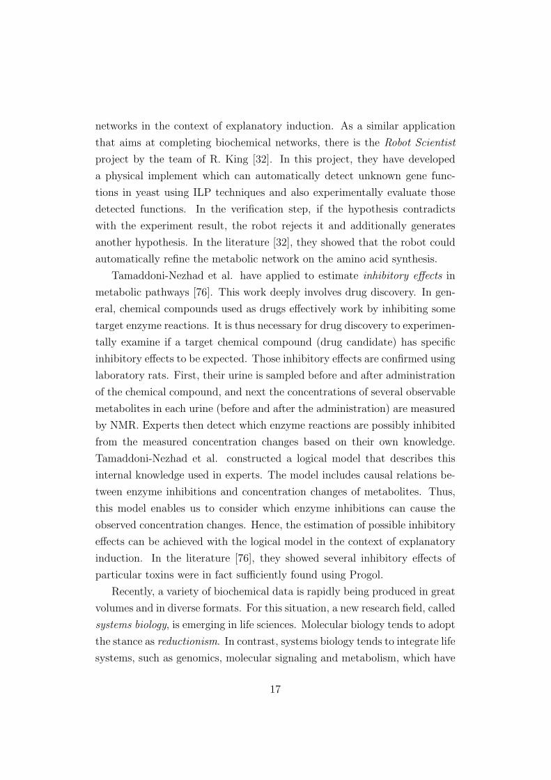
Tamaddoni-Nezhad et al. have applied to estimate inhibitory effects in
metabolic pathways [76]. This work deeply involves drug discovery. In gen-
eral, chemical compounds used as drugs effectively work by inhibiting some
target enzyme reactions. It is thus necessary for drug discovery to experimen-
tally examine if a target chemical compound (drug candidate) has specific
inhibitory effects to be expected. Those inhibitory effects are confirmed using
laboratory rats. First, their urine is sampled before and after administration
of the chemical compound, and next the concentrations of several observable
metabolites in each urine (before and after the administration) are measured
by NMR. Experts then detect which enzyme reactions are possibly inhibited
from the measured concentration changes based on their own knowledge.
Tamaddoni-Nezhad et al. constructed a logical model that describes this
internal knowledge used in experts. The model includes causal relations be-
tween enzyme inhibitions and concentration changes of metabolites. Thus,
this model enables us to consider which enzyme inhibitions can cause the
observed concentration changes. Hence, the estimation of possible inhibitory
effects can be achieved with the logical model in the context of explanatory
induction. In the literature [76], they showed several inhibitory effects of
particular toxins were in fact sufficiently found using Progol.
Recently, a variety of biochemical data is rapidly being produced in great
volumes and in diverse formats. For this situation, a new research field, called
systems biology, is emerging in life sciences. Molecular biology tends to adopt
the stance as reductionism. In contrast, systems biology tends to integrate life
systems, such as genomics, molecular signaling and metabolism, which have
17
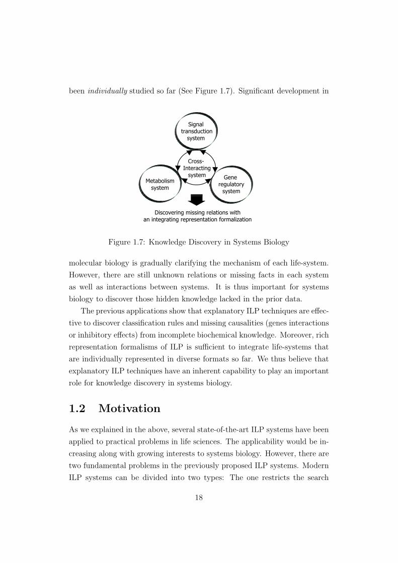
been individually studied so far (See Figure 1.7). Significant development in
Metabolismsystem
Gene regulatory
system
Signal transduction
system
Cross- Interacting
system
Discovering missing relations withan integrating representation formalization
Figure 1.7: Knowledge Discovery in Systems Biology
molecular biology is gradually clarifying the mechanism of each life-system.
However, there are still unknown relations or missing facts in each system
as well as interactions between systems. It is thus important for systems
biology to discover those hidden knowledge lacked in the prior data.
The previous applications show that explanatory ILP techniques are effec-
tive to discover classification rules and missing causalities (genes interactions
or inhibitory effects) from incomplete biochemical knowledge. Moreover, rich
representation formalisms of ILP is sufficient to integrate life-systems that
are individually represented in diverse formats so far. We thus believe that
explanatory ILP techniques have an inherent capability to play an important
role for knowledge discovery in systems biology.
1.2 Motivation
As we explained in the above, several state-of-the-art ILP systems have been
applied to practical problems in life sciences. The applicability would be in-
creasing along with growing interests to systems biology. However, there are
two fundamental problems in the previously proposed ILP systems. Modern
ILP systems can be divided into two types: The one restricts the search
18

space due to computational efficiency. The other ensures the completeness
in hypothesis finding, though it has to deal with a huge search space.
The first problem is involved in the former incomplete systems. Every
incomplete system has an inherent possibility that there is another hidden
hypothesis such that is more beneficial than the actual output. In this sense,
those systems make it difficult to guarantee the validity of their solutions. In
life sciences, we need to experimentally evaluate the generated hypothesis.
If ILP systems do not ensure the validity of their outputs, they cannot be
positively accepted by cagy experts who have to pay the costs, which are often
quite expensive. Incompleteness of hypothesis finding can make it restrained
to apply ILP systems in life sciences. Thus, it becomes necessary to overcome
the problem caused in incomplete ILP systems.
This problem never occurs in the latter complete systems. On the other
hand, those systems have to deal with a huge search space for preserving com-
pleteness in hypothesis finding. Such complete systems are used to consist
of non-deterministic procedures. Each non-deterministic procedure makes
many choice points where users have to select relevant one by hand. This
fact makes it difficult to apply them to practical problems that deal with a
large amount of data. The second problem lies in the non-determinisms of
the complete systems.
In this thesis, we first provide a practical example in systems biology that
the previously proposed incomplete systems cannot solve. That is because
this example needs an advanced inference technique that simultaneously in-
tegrates abduction and induction. The expected solutions are in the form of
abductive and inductive hypotheses in the context of explanatory induction.
For this task, we also show CF-induction, which is a complete explanatory
ILP method, efficiently works together with several interactions to users.
Most of the modern explanatory ILP methods are based on the prin-
ciple of Inverse Entailment (IE). This principle uses the following formula
equivalent to Formula (1.1) in the two conditions of explanatory induction:
B ∧ ¬E |= ¬H, (1.5)
where B, E and H denote a background theory, observations and a hypoth-
19

esis, respectively. Formula (1.5) means that for any hypothesis, its negation
can be derived from the background theory and the negation of observations
with entailment. Every IE-based method is used to compute hypotheses in
two steps: by first constructing an intermediate theory F such that
B ∧ ¬E |= · · · |= F |= · · · |= ¬H (1.6)
and next by generalizing its negation ¬F into the hypothesis H with the
inverse relation of entailment H |= ¬F .
Non-deterministic procedures in complete ILP systems mainly arise in
those two tasks: construction of an intermediate theory and generalization of
its negation. Both tasks involve in the problem how to realize the entailment
relation. Given a background theory B and observations E, there are many
possible intermediate theories to be constructed, each of which is derived
from B ∧ ¬E with the entailment relation. Moreover, for some constructed
theory F , there are also many possible hypotheses to be generated, each of
which is derived from ¬F with the inverse relation of entailment.
This thesis thus considers the issue on how those two tasks can be log-
ically simplified, while completeness in hypothesis finding is preserved. We
first focus on the sequence of intermediate theories that constructs a deriva-
tion from B∧¬E to ¬H in Formula 1.6. We then show the negations of those
intermediate theories can be represented with inverse subsumption. This log-
ical reduction enables us to use the subsumption relation in generalization,
instead of entailment, without losing the completeness. Based on this result,
we next logically reconstruct the current procedure of CF-induction into a
more simplified form. For its theoretical advantage preserving the complete-
ness, CF-induction potentially has plenty of practical applications in systems
biology like our motivating example. On the other hand, it required users
interactions each of which has to be selected one from many choice points
by hand. This fact has held the practical applications of CF-induction back.
By logically simplifying the current procedure, the non-determisims in CF-
induction can be reduced, and thus it would become possible to automatically
compute sufficient hypotheses that users wish to obtain.
20
1.3 Contribution
The contribution mainly consists of the following three works:
• The first contribution is to show new applicability of ILP techniques in
life sciences [88, 86, 13]. We provide a new practical example in systems
biology that cannot be solved by the previously proposed incomplete
systems. This example shows one limitation of those incomplete sys-
tems as well as the necessity of somehow ensuring the validity of the
generated hypothesis. The task in this example is achieved by an ad-
vanced inference integrating abduction and induction. We also show
how this task can be performed using CF-induction.
• The second contribution is to prove that the complete generalization
in the IE-based methods can be achieved by inverse relation of sub-
sumption [90]. Previously, it has been known that the generalization
based on the entailment relation can ensure completeness in hypothe-
sis finding. However, this procedure needs to consist of many so-called
generalization operators such as inverse resolution. Each generalization
operator has many ways to be applied and any combination of them
is also applied as another generalization operator. This fact makes the
generalization procedure highly non-determinisitc. For this problem,
we show inverse subsumption, instead of entailment, is sufficient to
ensure the completeness in generalization.
• The third contribution is to logically reconstruct the procedure of CF-
induction into a more simplified form [91, 92]. Like other IE-based
methods, CF-induction consists of two procedures: construction of in-
termediate theories and generalization of its negation. In the previous
CF-induction, each procedure required several users interactions where
some relevant one should be selected from many choice points. In con-
trast, we first show a deterministic procedure to construct intermediate
theories, while our proposal does not lose any completeness in hypoth-
esis We next propose two possible approaches for generalization task.
21

The first approach is based on the logical relation between the nega-
tion of an intermediate formula and a hypothesis. This logical relation
can be realized with inverse subsumption using the result is the second
contribution. Alternatively, the second approach is based on the logical
relation between an intermediate formula and the negation of a hypoth-
esis. Compared with the first approach, the second approach actively
uses deductive inference. We thus show that in both approach, the
non-determinism in generalization can be dramatically reduced. We
also consider efficient implementation in CF-induction [89].
In summary, the thesis shows new applicability of inference-based hypothesis-
finding techniques in life sciences as well as essential limitations in the previ-
ously proposed ILP methods. The thesis also provides us fundamental prop-
erties in hypothesis finding that can be commonly applied in the IE-based
explanatory ILP methods, and also propose sound and complete procedures
obtained by logically simplifying CF-induction. We believe that the contents
shown in the thesis would give us underlying nature and insights to clarify
the logic and computation in hypothesis finding.
1.4 Overview
The rest of this thesis is organized as follows. Chapter 2 reviews the notions
and terminologies in this thesis, which include the syntax and semantics in
first-order logic, clausal forms and consequence finding as well as the dual-
ization problem. Chapter 3 reviews the principle of inverse entailment and
introduces each previously proposed hypothesis-finding method based on in-
verse entailment including CF-induction. Chapter 4 provides a new practical
application in systems biology. Its task is to find both abductive and induc-
tive hypothesis that can complete the prior background theory. We show
how this advanced inference can be realized using CF-induction. The con-
tent in Chapter 4 corresponds to the first contribution in the previous section.
Chapter 5 shows that the generalization relation in hypothesis finding based
on inverse entailment can be reduced to inverse subsumption. The content in
Chapter 5 corresponds to the second contribution in the previous section. In
22

Chapter 6, we focus on the current procedure of CF-induction and logically
reconstruct each non-deterministic procedure into a more simplified one. We
also discuss about efficient implementation of CF-induction with considera-
tion of issues concerning the non-monotone dualization problem. Chapter 7
concludes and describes future works.
1.5 Publications
The referred publications are as follows:
1. Yoshitaka Yamamoto, Katsumi Inoue and Koji Iwanuma. From inverse entailment
to inverse subsumption. Proceedings of the 20th Int. Conf. on Inductive Logic
Programming, to appear, 2010 [90].
2. Yoshitaka Yamamoto, Katsumi Inoue and Koji Iwanuma. Hypothesis enumeration
by CF-induction. Proceedings of the Sixth Workshop on Learning with Logics and
Logics for Learning (LLLL2009), pages 80-87. The Japanese Society for Artificial
Intelligence, 2009 [89].
3. Yoshitaka Yamamoto, Katsumi Inoue and Andrei Doncescu. Integrating Abduction
and Induction in Biological Inference using CF-Induction. Huma Lodhi and Stephen
Muggleton (eds.), Elements of Computational Systems Biology, Wiley Book Series
on Bioinformatics, pages 213-234, John Wiley and Sons, Inc., 2009 [88].
4. Yoshitaka Yamamoto, Katsumi Inoue and Andrei Doncescu. Abductive reasoning
in cancer therapy. Proceedings of the 23rd Int. Conf. on Advanced Information
Networking and Applications(AINA 2009), pages 948-953. IEEE Computer Society,
2009 [87]. This paper deals with another biological application of our ILP system
based on SOLAR. In this thesis, we do not include the content of this paper.
5. Yoshitaka Yamamoto, Oliver Ray and Katsumi Inoue. Towards a logical reconstruc-
tion of CF-induction. K. Satoh, A. Inokuchi, K. Nagao and T. Kawamura (eds.),
In New Frontiers in Artificial Intelligence: JSAI 2007 Conference and Workshop
Revised Selected Papers, Lecture Notes in Artificial Intelligence, volume 4914, pages
330-343, Springer, 2008 [92].
23

6. Yoshitaka Yamamoto and Katsumi Inoue. An efficient hypothesis-finding system
implemented with deduction and dualization. Proceedings of the 22nd Workshop
on Logic Programming (WLP 2008), pages 92-103. University Halle-Wittenberg
Institute of Computer Science Technical Report, 2008 [85].
7. Yoshitaka Yamamoto, Katsumi Inoue and Andrei Doncescu. Estimation of possible
reaction states in metabolic pathways using inductive logic programming. Proceed-
ings of the 22nd Int. Conf. on Advanced Information Networking and Applications
(AINA 2008), pages 808-813. IEEE Computer Society, 2008 [86].
8. Yoshitaka Yamamoto, Oliver Ray and Katsumi Inoue. Towards a logical reconstruc-
tion of CF-Induction. Proceedings of the 4th Workshop on Learning with Logics and
Logics for Learning (LLLL 2007), pages 18-24, The Japanese Society for Artificial
Intelligence, 2007 [91].
9. Andrei Doncescu, Katsumi Inoue and Yoshitaka Yamamoto. Knowledge-based dis-
covery in systems biology using CF-induction. New Trends in Applied Artificial
Intelligence: Proceedings of the 20th Int. Conf. on Industrial, Engineering and
Other Applications of Applied Intelligent Systems (IEA/AIE 2007), Lecture Notes
in Artificial Intelligence, volume 4570, pages 395-404, Springer, 2007 [13].
10. Andrei Doncescu, Yoshitaka Yamamoto and Katsumi Inoue. Biological systems
analysis using Inductive Logic Programming. Proceedings of the 21st Int. Conf. on
Advanced Information Networking and Applications (AINA 2007), pages 690-695,
IEEE Computer Society, 2007 [14].
24

Chapter 2
Preliminaries
This chapter reviews the notion and terminology that are used throughout
the thesis. Section 2.1 describes the syntax and semantics in the first-order
logic as well as its prenex normal and clausal forms (Skolem standard forms).
We next review the resolution principle in Section 2.2. In this section, we
also introduce several important theorems such as Herbrand’s theorem and
Subsumption theorem. Much of Section 2.1 and 2.2 is adopted from [7, 52, 59].
Section 2.3 describes issues on the dualization problem to translate a given
conjunctive normal form formula into a logically equivalent disjunctive (resp.
conjunctive) normal form formula. Note that dualization plays an important
role in hypothesis finding based on the principle of inverse entailment.
2.1 First-Order Logic
Through this thesis, we represent the logical formulas using the classical
first-order predicate logic. Here, we formally define this representation for-
malization. Then, we start with the syntax of first-order logical formulas,
which is formalized with an alphabet of the first-order logic language L de-
fined below.
Definition 2.1. An alphabet of the first-order logic consists of the following
symbols:
• A set of constant symbols: {“a”, “b”, “c”, . . . }.
25

• A set of variable symbols: {“x”, “x1”, “y”, . . . }.
• A set of function symbols: {“f”, “f1”, “g”, . . . }.
• A set of predicate symbols: {“p”, “p1”, “q”, . . . }.
• The logical symbols: “∀”, “∃”, “¬”, “ ∧ ”, “ ∨ ” and “ → ”.
• The punctuation symbols: “(”, “)” and “, ”.
The two logical symbols “∀” and “∃” are called the quantifiers, respec-
tively. The other logical symbols are called the connectives. Every function
and predicate symbol has a certain number of arguments, called its arity. In
particular, function and predicate symbols of arity zero are called constant
and proposition symbols, respectively.
Definition 2.2. Well-formed expressions are constructed as follows:
1. A term is either a variable x, a constant c or a function f(t1, . . . , tn) of
arity n ≥ 1 where t1, . . . , tn are terms.
2. A atom is a predicate p(t1, . . . , tn) of arity n ≥ 0 where t1, . . . , tn are
terms. In the case of n = 0, p() will be simply be written p.
3. A formula is either an atom, a universal (∀x)φ, an existential (∃x)φ,
a negation (¬φ), a conjunction (φ ∧ ψ), a disjunction (φ ∨ ψ), an im-
plication (φ → ψ), where x is a variable and φ and ψ are formulas.
Especially, the equivalence formula (φ → ψ) ∧ (ψ → φ) is simply writ-
ten φ ↔ ψ.
An expression is called ground iff no variables appear in the expression.
Let φ be a formula. Then, two formulas (∀x)φ and (∃x)φ are said to be
universally and existentially quantified in x, respectively. φ is said to be
the scope of ∀x and ∃x in (∀x)φ and (∃x)φ, respectively. An occurrence of
a variable x in a formula is bound if the occurrence immediately follows a
quantifier or it lies within the scope of some quantifier that is immediately
followed by x. An occurrence of a variable which is not bound, is called free.
For example, the first occurrence of x in ((∃x)Q(x) ∨ P (x, f(a)) is bound,
26
whereas the second occurrence of x is free. A formula is closed if it does
not contain any free occurrences of variables. The first-order language given
by an alphabet is the set of all the well-formed expressions which can be
constructed by the alphabet. In the following, we will not explicitly specify
the alphabet used in each example. Instead, we assume that the alphabet
includes all the symbols we use in the example. In addition, we assume that
every formula is closed, i.e. it has no free variables.
The meaning of each expression in a first-order language like terms, func-
tions and predicates is given by considering what it refers to or whether or
not it is true. Hence, the meanings of expressions depend on what the domain
of discourse we assume and how we interpret expressions over the domain.
The following is the formal definition of an interpretation of the expressions
in a given first-order language.
Definition 2.3. Let L and D be a first-order language and a nonempty
domain of discourse. An interpretation I wrt L and D consists the following
three assignments to each constant, function and predicate occurring in F :
1. To each constant c, we assign an element cI in D.
2. To each function f of arity n ≤ 1, we assign a function f I : Dn → D,
where Dn = {(x1, . . . , xn) | x1 ∈ D, . . . , xn ∈ D}.
3. To each predicate p of arity n ≤ 0, we assign a relation pI ⊆ Dn.
(Note that in case that n = 0, D0 denotes a set that includes only one
element.)
Given an interpretation in a first-order language L over a domain D,
it is further necessary to associate each variable to some element in D for
determining the value of every expression in L. We define this as follows:
Definition 2.4. Let L and D be a first-order language and a nonempty
domain. A variable assignment h wrt L and D is a mapping from the set of
variables in L to the domain D.
Let h and I be a variable assignment and an interpretation wrt a given
first-order language L and domain D.
27

The value of a term t in I under h is determined by the function [t]I,h from
the terms of L to D, defined as follows:
• [c]I,h = cI , for a constant c;
• [x]I,h = h(x), for a variable x;
• [f(t1, . . . , tn)]I,h = f I([t1]I,h, . . . , [tn]I,h), for a function f of arity n ≥ 1.
The truth of a formula F in I under h is determined by the relation I, h |= F
over the formulas in L, defined as follows:
• I, h |= p(t1, . . . , tn) iff ([t1]I,h, . . . , [tn]I,h) ∈ pI , for a predicate p;
• I, h |= (F → G) iff I, h 6|= F or I, h |= G;
• I, h |= (F ∨ G) iff I, h |= F or I, h |= G;
• I, h |= (F ∧ G) iff I, h |= F and I, h |= G;
• I, h |= (¬F ) iff I, h 6|= F ;
• I, h |= (∃x)F iff I, hx/d |= F for some d ∈ D, where hx/d is the variable
assignment such that if x = y then hx/d(y) = d, otherwise hx/d(y) =
h(y).
• I, h |= (∀x)F iff I, hx/d |= F for every d ∈ D.
F be a formula in the language. The relation I, h |= F means F is true in
the interpretation I under the variable assignment h. An interpretation M
is a model of a formula F iff M,h |= F for every variable assignment h. F is
satisfiable (or consistent) iff there is a model of F . If F is not satisfiable, F
is called a contradiction (or inconsistent). F is tautology (or valid) iff every
interpretation is a model of F .
Let Σ be a set of formulas in the language. An interpretation M is a
model of Σ iff M is a model of every formula in Σ. Σ (logically) entails a
formula F , denoted Σ |= F , iff every model of Σ is a model of F . We call F
a logical consequence of Σ. If F is not a logical consequence of Σ, then we
28

write Σ 6|= F . In case that Σ = {G} for some formula G, we simply write
G |= F . Σ (logically) entails a set of formulas Γ, denoted Σ |= Γ, iff every
model of Σ is a model of every formula in Γ. If not Σ |= Γ, we write Σ 6|= Γ.
Two formulas F and G are said to be (logically) equivalent, denoted F ≡ G,
iff both F |= G and G |= F . Similarly, two sets of formulas Σ and Γ are said
to be logically equivalent, denoted Σ ≡ Γ, iff both Σ |= Γ and Γ |= Σ.
Let L be the set of all formulas in the language. Then, the notion of logical
entailment can be viewed as a binary relation |= ⊆ 2L × 2L. It is known that
the entailment relation |= satisfies the following features: (reflexivity) Σ1 |=Σ1, (transitivity) if Σ1 |= Σ2 and Σ2 |= Σ3 then Σ1 |= Σ3, (monotonicity)
if Σ1 |= G then Σ1 ∪ {F} |= G; (cut) if Σ1 |= F and Σ1 ∪ {F} |= G then
Σ1 |= G; (deduction) Σ1 ∪ {F} |= G iff Σ1 |= F → G; and (contraposition)
Σ1 ∪ {F} |= G iff Σ1 ∪ {¬G} |= ¬F , for each formulas F and G and each
set of formulas Σ1, Σ2 and Σ3. Especially, we denote by 2 the empty set of
formulas. Since there is no models of 2, it holds that a set Σ of formulas is
inconsistent iff Σ |= 2 holds. Accordingly, it holds that for every two sets Σ1
and Σ2, Σ1 ∪ Σ2 is inconsistent iff Σ1 ∪ Σ2 |= 2. Using this property as well
as the contraposition, we often denote by Σ1 |= ¬Σ2 that Σ1 is inconsistent
with Σ2. Hence, the consistency condition of two sets Σ1 and Σ2 can be
represented by Σ1 6|= ¬Σ2.
The entailment relation is an important concept in logic-based artificial
intelligence. Once we represent the knowledge in a target system with a first-
order language, the entailment relation enables us to obtain new statements
that the prior knowledge does not refer to. On the other hand, given a set
of formulas Σ, we may not be able to find out in finite time whether or not
Σ |= F holds for some formula F , since the number of possible interpretations
is usually infinite. We will review some related issues on this consequence
finding problem in Section 2.3. As its introduction, we define several normal
forms like clausal forms in next section.
29

2.2 Normal Forms and Herbrand’s Theorem
In the previous section, we reviewed the syntax and semantics in first-order
logic. Given a first-order language L, every formula in L has several alter-
native representation formalizations. For instance, the formula ¬((∃x)f(x))
is logically equivalent to the formula (∀x)f(x). In this section, we introduce
several standard forms for representing the formulas in the language L.
Definition 2.5 (Prenex normal forms). A formula F is said to be in prenex
normal form iff the formula F is the form of
(Q1x1) · · · (Qnxn)(M).
where every Qixi (1 ≤ i ≤ n), is either (∀xi) or (∃xi), and M is a formula
containing no quantifiers. (Q1x1) · · · (Qnxn) is called the prenex and M is
called the matrix of the formula F .
It is well known that for every formula F , there exists a formula F ′ in
prenex normal form such that F is logically equivalent to F ′ and an equiv-
alent formula F ′ can be obtained by translating F with several equivalent
translating operations [52, 7].
We next define so-called Skolem standard forms, which was introduced
by Davis and Putnam [10]. Every formula F in the language is translated
into its prenex normal form (Q1x1) · · · (Qnxn)(M) without lose of general-
ity. The matrix M , since it does not contain quntifiers, can be transformed
into a conjunctive normal form. After this transformation, we eliminate
the existential quantifiers in the prenex by using Skolem functions. We of-
ten say this as skolemizing the formula F , which follows the below opera-
tions. Suppose Qr (1 ≤ r ≤ n) is an existential quantifier in the prenex
(Q1x1) · · · (Qnxn). If no universal quantifier appears before Qr, we choose a
new constant c different from other constants occurring in M , replace all xr
appearing in M by c, and delete (Qrxr) from the prefix. If Qs1 , Qs2 . . . , Qsm
(1 ≤ s1 < s2 < · · · < sm < r) are all the universal quantifiers appearing be-
fore Qr, we choose a new function f of arity m different from other functions,
replace all xr in M by f(xs1 , xs2 , · · · , xsm), and delete (Qrxr) from the pre-
fix. After the above process is applied to all the existential quantifiers in the
30

prenex, the last formula we obtain is a Skolem standard form of the formula
F . The constants and functions used to replace the existential variables are
called Skolem functions.
Every formula can be put in the Skolem standard form, but not every
formula has a standard form which is equivalent to the original formula.
For example, using the above translating procedure, the formula (∃x)F (x)
is translated to the Skolem standard form F (c) for a new constant c. The
original formula implies that there is an element in the extension of the
predicate F . In contrast, the translated standard form formula implies that
an element associated with the term c is in the extension of the prediacate
F . If the latter is true, then the former is true. However, its inverse does not
necessarily hold. Hence, the translation into Skolem standard forms can lose
the generality. On the other hand, it can affect the inconsistency property
in the original formula. Let F be a formula and FS a Skolem standard form
of F . Then it is known that F is inconsistent iff FS is inconsistent.
This feature is a strong evidence to use Skolem standard forms in auto-
mated theorem proving. The task in theorem proving is to decide whether
or not Σ |= F for a given set of formulas Σ and a target formula F . If
true, Σ ∪ {¬F} should be inconsistent by the contrapositive property of the
entailment relation. Hence, it is sufficient for the original task to check the
inconsistency of a Skolem standard form of Σ ∪ {¬F}.For two Skolem standard form formulas, the difference between them
occurs only in the part of matrixes. Their matrixes are formalized in con-
junctive normal forms which are alternatively defined using the notion of
clauses. A literal is an atom or the negation of an atom. A positive lit-
eral is an atom, a negative literal is an atom. A clause is a finite disjunc-
tion of literals which is often identified with the set of its literals. A clause
{A1, . . . , An,¬B1, . . . ,¬Bm}, where each Ai, Bj is an atom, is also written as
B1 ∧ · · · ∧ Bm ⊃ A1 ∨ · · · ∨ An. A definite clause is a clause which contains
only one positive literal. A positive (negative) clause is a clause whose dis-
juncts are all positive (negative) literals. A Horn clause is a definite clause
or negative clause. A unit clause is a clause with exactly one literal. The
empty clause, denoted ⊥, is the clause which contains no literals.
31

A clausal theory is a finite set of clauses. Note that a clausal theory S can
include tautological clauses. Then, τS denotes the set of non-tautological
clauses in S. A clausal theory is full if it contains at least one non-Horn
clause. A conjunctive normal form (CNF) formula is a conjunction of clauses,
and a disjunctive normal form (DNF) is a disjunction of conjunctions of
literals. A clausal theory S is often identified with the conjunction of its
clauses. In this thesis, every variable in a clausal theory S is considered
governed by the universal quantifier. By this convension, a Skolem standard
form can be simply represented by a clausal theory.
For the sake of simplicity and preserving inconsistency of original formu-
las, clausal forms have been commonly used for knowledge representation in
automated reasoning with first-order logic.
Let S be a clausal theory. Then, how can we check whether or not S
is inconsistent? Based on the primary definition of the entailment relation,
it is necessary to check all the interpretations with respect to every possi-
ble domains, which cannot be achieved in real. For this problem, Herbrand
introduced a specific model, called a Herbrand model, and proved an impor-
tant feature that inconsistency of clausal theories can be checked within the
notion of Herbrand models. As a preliminary, we define several key notions
in the below. Let S be a clausal theory. The Herbrand universe, denoted
HS, is the set of all ground terms in S. Note that if no ground term exists
in S, US consists of a single constant c, say HS = {c}. The Herbrand base,
denoted BS, is the set of all ground atoms in S.
Let AS be the alphabet consisting of the constants, variables, functions,
and predicates symbols in S. Then, we denote the first-order language given
by the alphabet AS by LS. A Herbrand interpretation IH of S is an inter-
pretation wrt the language LS and the domain US such that cIH = c for
each constant c in LS, f IH = f for each function f in LS, and pIH ⊆ UnS
for each predicate p in LS. Let S be a clausal theory and IH a Herbrand
interpretation of S. IH is a Herbrand model iff IH satisfies S. It is known
that for a clausal theory S, S has a model iff S has a Herband model. This
property enables us to focus on only the Herbrand models for checking the
inconsistency of S.
32

Let S be a clausal theory. A ground instance of a clause C in S is a clause
obtained by replacing variables in C by members of the Herbrand universe
US of S. If S has a model, by the property of Herbrand models, S has also a
Herbrand model. In other other, S is true in some Herbrand interpretation
IH of S for every variable assignment h. Note that each variable assignment
h maps the set of variables in S into members in the Herbrand universe
US. Then, this mapping can be regarded as constructing ground instances
of clauses in S. Hence, if S has a model, every finite set of ground instances
of clauses in S should be also true in some Herbrand interpretation IH . By
taking the contrapositive of this statement, if there is a finite set S ′ of ground
instances of clauses in S such that S ′ is false in every Herbrand interpretation
IH (that is, S ′ is inconsistent), then S does not have any model (that is, S
is inconsistent). Interestingly, this inverse also holds, which Herbrand has
firstly proved.
Theorem 2.1 (Herbrand’s theorem). Let S be a clausal theory. S is incon-
sistent iff there is a finite set of ground instances of clauses in S.
2.3 Consequence Finding
In the previous section, we introduced clausal forms that are commonly used
in Inductive Logic Programming as well as Herbrand’s theorem. One im-
portance issue that this theorem brings is the fact that the consistency of a
target clausal theory can be systematically decided by checking the consis-
tency of each possible finite set S ′ of ground instances from S. The consis-
tency of each S ′ can be determined in the finite number of checking. This
propositional approach based on Herbrand’s theory is one possible way to
realistically achieve the task of automated theorem proving. Given a clausal
theory S, the essential problem in automated deductive reasoning lies in how
we can find the logical consequences of S. In case that S is inconsistent, this
problem is reduced to find the refutation, that is, the empty clause. For the
consequence finding problem, it is difficult to use the propositional approach
since logical consequences are not necessarily ground. Instead, we can use
so-called resolution principle, which was introduced by Robinson. In this
33

section, we first define key notions such as substitutions and subsumption,
next describe the resolution principle in brief, and lastly introduce the Sub-
sumption theorem which shows the completeness of the resolution principle
for consequence finding.
Let C and D be two clauses. C subsumes D, denoted C º D, if there
is a substitution θ such that Cθ ⊆ D. C properly subsumes D if C º D
but D 6º C. For a clausal theory S, µS denotes the set of clauses in S not
properly subsumed by any clause in S. Let S1 and S2 be two clausal theories.
S1 subsumes S2, denoted S1 º S2 iff for any clause D ∈ S2, there exists a
clause C ∈ S1 such that C º D. In particular, S1 strongly subsumes S2,
denoted S1 º\ S2 iff S1 º S2 and for any clause C ∈ S1, there exists a clause
D ∈ S2 such that C º D. the relation º\ is known as Plotkin’s order [56]
Let C1 and C2 be two clauses (called parent clauses) with no variables in
common. Let L1 and L2 be two literals in C1 and C2, respectively. If L1 and
¬L2 have a most general unifier σ, then the clause
(C1σ − {L1σ}) ∪ (C2σ − {L2σ})
is called a (binary) resolvent of C1 and C2, denote Res(C1, C2). The literals
L1 and L2 are called the literals resolved upon. Let S be a clausal theory
and C be a clause. A derivation of C from S is a finite sequence of clauses
R1, . . . , Rk = C such that each Ri is either in S, or is a resolvent of two clauses
in R1, . . . , Ri−1. S is minimal wrt derivation iff for each clause C ∈ S, there
is no D such that a derivation from S − {C} can be constructed to D and
D º C. S is maximal wrt derivation iff for each consequence C of S, there
exists a clause D in S such that D º C.
We then recall the following result, called the Subsumption theorem.
Theorem 2.2 ([37, 52]). Let S be a clausal theory and C be a clause. Then
S |= C iff C is a tautology or there exists a derivation of a clause D from S
that subsumes C.
For a clausal theory S, a consequence of S is a clause entailed by S
as we defined in the previous section. We denote by Th(S) the set of all
34

consequences of S. The Subsumption theorem states the completeness of the
resolution principle for finding any non-tautological consequences in µTh(S).
By the Subsumption theorem, the resolution principle is sufficient to com-
pute the non-tautological consequences µTh(S) for a target clausal theory
S. SLD resolution [38] is a well known deduction technique as the key pro-
cedure in Prolog. Though SLD resolution can be used to theorem proving,
we cannot use it for consequence finding. Besides, though SLD resolution
preserves the soundness and completeness for finding refutations, its usage
is limited in Horn representation formalization. Inoue [25] proposed to use
a restricted but powerful consequence finding technique to overcome this
problem. The essential idea lies in so-called characteristic clauses, which are
“interesting” consequences that users wish to obtain. Characteristic clauses
are declaratively defined with a language bias, called a production field. Us-
ing a relevant production field, we can efficiently restrict the search space for
hypothesis finding. We first formally define the key notions as follows:
A production field P is defined as a pair, 〈L,Cond〉, where L is a set
of literals closed under instantiation, and Cond is a certain condition to be
satisfied, e.g., the maximum length of clauses, the maximum depth of terms,
etc. Note that if L is closed under instantiation. A production field P is
stable if for any two clauses C and D such that C subsumes D, D belongs to
P only if C belongs to P . For instance, the production field P = 〈{p(a)}〉 is
not stable, since there is a clause p(X) such that p(X) does not belong to P ,
but the ground clause p(a) that is subsumed by p(X) belong to P . Note that
there is recent a work to make any unstable production fields stable [62].
Let R be the set of all predicate symbols appeared in the language. For
R ⊆ R, we denote by R+ (R−) the positive (negative) occurences of predi-
cates from R in the language.
A clause C belongs to P = 〈L,Cond〉 if every literal in C belongs to L
and C satisfies Cond. For a set S of clauses, the set of consequences of S
belonging to P is denoted by ThP(S). Then, the characteristic clauses of S
wrt P are defined as:
Carc(S,P) = µThP(S)
Note that Carc(S,P) can, in general, include tautological clauses [25].When
35

Cond is not specified, P is simply denoted as 〈L〉. If both L and Cond are not
specified, P , denoted as 〈L〉, allows all the formulas in the first-order language
L. Note that for the production field P = 〈L〉, Carc(S,P) = µTh(S).
Example 2.1. Let a clausal theory S and a (stable) production field P be
as follows:
S = {s(X0), p(X1) ∨ ¬q(X1) ∨ ¬s(Y1), p(X2) ∨ q(X2) ∨ r(X2)},
P = 〈{±p, ±q, ±r}, max length ≤ 3〉.
Note that for a predicate symbol p of arity k, ±p means the complementary
literals p(X1, . . . , Xk) and ¬p(X1, . . . , Xk) and the condition max length ≤ k
for some natural number k means the number of literals in every characteristic
clauses is less than or equal to k. Using the resolution principle, we have three
additional consequences derived from S :
C1 = p(X3) ∨ ¬q(X3), C2 = p(X4) ∨ r(X4) ∨ ¬s(Y1), C3 = p(X5) ∨ r(X5).
Whereas the number of literals in every clause in S and those three clauses
is less than or equal to 3, only C1, C3 and the 3rd clause in S belong to Pas the other contains the predicate s that is not allowed to be included. In
addition, the following tautological clauses also belong to P:
C4 = p(X6) ∨ ¬p(X6), C5 = q(X7) ∨ ¬q(X7), C6 = r(X8) ∨ ¬r(X8).
Then, ThP(S) consists of those 6 clauses. On the other hand, both the
3rd clause in S and C2 are properly subsumed by C3. As a result, the
characteristic clauses of S wrt P are only C1, C3, C4, C5 and C6.
When a new clause F is added to a clausal theory, some consequences are
newly derived with this additional information. The set of such clauses that
belong to the production field are called new characteristic clauses . Formally,
the new characteristic clauses of F wrt S and P are defined as:
NewCarc(S, F,P) = Carc(S ∪ {F},P) − Carc(S,P).
36
Example 2.2. Recall Example 2.1. Let a new clause F be ¬p(Z1). Then,
ThP (S ∪ {F}) consists of ThP(S) and the following three consequences de-
rived from S together with F :
C7 = ¬q(Z1) ∨ ¬s(Y1), C8 = q(Z1) ∨ r(Z1), C9 = ¬q(Z2), C10 = r(Z3).
Since C9 properly subsumes both C7 and C8, it holds that Carc(S∪{F},P) =
µ[{C9, C10} ∪ ThP(S)]. Hence, NewCarc(S, F,P) consists of C9 and C10.
For computation of the (new-)characteristic clauses, Inoue [25] proposed
a sound and complete resolution procedure, called SOL resolution. SOL
resolution constructs derivations from F with respect to S based on three
inference rules: Skip, Extension and Reduction. Note that SLD resolution
consists of Extension and Reduction operations. Hence, SOL resolution can
be regarded as an extension of SLD resolution constructed by adding Skip
operation to SLD resolution.
Let S be a clausal theory and F a clause. We call a derivation obtained
by SOL resolution as an SOL-deduction from S + F and P .
Theorem 2.3 (The soundness and completeness of SOL-deductions [29]).
The soundness and completeness of SOL-deductions are formally described
as follows:
1. Soundness: if a clause D is derived by an SOL-deduction from S + F
and P , then D belongs to ThP(S ∪ {F}).
2. Completeness: if a clause E does not belong to ThP(S) but belongs
to ThP(S ∪ {F}), then there is an SOL-deduction of a clause D from
S + F and P such that D subsumes E.
In terms of efficient implementation on SOL resolution, there is an avail-
able system, called SOLAR [29, 51]. SOLAR (SOL for Advanced Reasoning)
uses a connection tableau format embedding the three operations to effi-
ciently compute new characteristic clauses.
Example 2.3. We recall Example 2.2. SOLAR constructs a SOL-deduction
of C10 = r(Z3) from S + F and P with the following tableau in Figure 2.1:
37

!
¬p(X)
!
p(X)
!
¬q(X)
!
¬s(X)
!
s(X)
(Extension)
!
p(X)
!
q(X)
!
r(X)
(Extension)(Extension)
(skip)* *
*
*
(Reduction)
Figure 2.1: Tableau in SOLAR
2.4 Dualization
In this section, we review issues on the dualization problem. The dualization
problem is a well-known problem in NP-completeness [16]. It needs huge com-
putational costs, whereas hypothesis finding techniques such as CF-induction
often need it. Thus, it is essential to use efficient algorithms for real-world ap-
plications of those hypothesis-finding techniques that use dualization. After
describing basic notion and terminologies, we introduce an efficient algorithm
in a specific dualization problem, called monotone dualization.
The dualization problem [15, 16, 68] is to compute a CNF formula from
the dual ψd of a given CNF formula ψ. Let ψ be a CNF formula. The
dual ψd is the DNF formula obtained by replacing every conjunction symbol
∧ (∨) with the disjunction symbol ∨ (∧) in ψ. Though there are many
CNF formulas equivalent to ψd in general, we are used to find a prime and
irredundant CNF formula. A CNF formula S is prime if for every C ∈ S,
there is no literal l ∈ C such that (S−{C})∪{C−{l}} ≡ S. A CNF formula
S is irredundant if there is no clause C ∈ S such that S − {C} ≡ S.
Example 2.4. Let ψ1 and ψ2 be as following CNF formulas:
ψ1 = (a ∨ b) ∧ (c ∨ ¬b) ∧ (a ∨ c),
ψ2 = (a ∨ b) ∧ (a ∨ ¬b).
ψ1 is prime, since for every literal l in ψ1, the clause obtained by dropping l is
no longer logically equivalent to ψ1. On the other hand, ψ1 is redundant, since
38
the third clause in ψ1 is the resolvent of the other two clauses. In contrast, ψ2
is irredundant, since for ever clause C in ψ2, ψ2 − {C} is no longer logically
equivalent to ψ2. On the other hand, ψ2 is non-prime, since two literals b
and ¬b can be dropped from ψ2 without losing the logical equivalence.
Let ψ be a CNF formula. ψ is monotone iff ψ does not include any nega-
tions. We call dualization of monotone CNF formulas as monotone dualiza-
tion. An arbitrary monotone CNF formula ψ satisfies two nice properties:
The first is that ψ has its unique prime CNF. The second is that if ψ is
prime, then ψ is irredundant. These two properties imply that the mono-
tone dualization problem is to finding the unique prime CNF formula. In
contrast, a non-monotone CNF formulas does not necessarily have its unique
prime-irreducndant CNF, shown as the following example:
Example 2.5. Let three CNF formula ψ1, ψ2 and ψ as follows:
ψ1 = (a ∨ b) ∧ (¬b ∨ c) ∧ (¬c ∨ ¬a),
ψ2 = (a ∨ c) ∧ (¬b ∨ ¬a) ∧ (¬c ∨ b),
ψ = ψ1 ∧ ψ2.
Both ψ1 and ψ2 are prime and irredundant CNF formulas logically equivalent
to ψ. Thus, the prime-irredundant CNF of ψ is not indeed unique.
It is well known that the monotone dualization is equivalent to the min-
imal hitting sets enumeration [17], which is solvable in quasi-polynominal
time [19]. We then here introduce an efficient algorithm [78, 68] for this
enumeration problem. To describe the algorithm, we first give the definition
of a minimal hitting set of a given family of sets.
Definition 2.6 ((Minimal) Hitting set). Let Π be a finite set and F be a
subset family of Π. A hitting set HS of F is a set such that for every S ∈ F ,
S ∩HS 6= ∅. A set MHS is a minimal hitting set of F if MHS satisfies the
following two conditions:
1. MHS is a hitting set of F ;
39

2. For every subset MHS ′ ⊆ MHS, if MHS ′ is a hitting set of F , then
MHS ′ = MHS.
As a property in minimal hitting sets, the following theorem holds:
Theorem 2.4. [78] Let F be a family of sets. A set E is a minimal hitting
set of F iff for every element e ∈ E, there exists a set F in F such that
E ∩ F = {e}.
Example 2.6. Let a monotone CNF formula ψ be (a∨b)∧(a∨c) and a subset
family Fψ {{a, b}, {a, c}}. Note that each set in Fψ can be identified with a
conjunction of ψ. We first show the correspondence between the dualization
of ψ and the miniminal hitting set enumeration of Fψ. The dual ψd is the
DNF (a∧ b)∨ (a∧ c). The prime implicants of ψd are two clauses a and b∨ c.
Then, the output of the dualization of ψ is the prime CNF φ = a ∧ (b ∨ c).
In contrast, the minimal hitting sets of Fψ contains two sets {a} and {b, c}.We then notice that each of which can be identified with a conjunction of φ.
This Fψ follows Theorem 2.4. When we consider the minimal hitting
set E1 = {a} of Fψ, there is in fact a set F1 = {a, b} ∈ Fψ such that
E1 ∩ F1 = {a}. When we consider another minimal hitting set E2 = {b, c},for each element b and c, there are two sets F1 = {a, b} and F2 = {a, c} in
Fψ such that E2 ∩ F1 = {b} and E2 ∩ F2 = {c}, respectively.
An efficient algorithm that we introduce here is based on the principle of
reverse search [2] for enumeration problems. In reverse search, we define a
relevant relation, called a parent-child relationship over the solution space (i.e.
the minimal hitting sets of a given subset family). Note that this relationship
has to satisfy the condition that for every solution, there is no ancestor on the
relationship, such that is equal to the original solution. Such a relationship
that satisfies this condition can lead a rooted-tree, called a enumeration tree,
on the solution space. In general, the size of an enumeration tree is too big to
store it in memory for searching. Instead, we use a relevant algorithm that
enables us to enumerate only the children of any node in the tree. Using
this algorithm, we can search all the solutions with the depth-first strategy,
40
while we do not need to store the whole enumeration tree in memory. The
parent-child relationship presented in [78] is defined as follows.
Definition 2.7 (Parent-child relationship [78]). Let Π be a finite set, Fn =
{F1, . . . , Fn} a subset family of Π that contains n elements and Ei (1 ≤ i ≤ n)
a minimal hitting set of Fi. Then a pair (i+1, Ei+1) is a child of a pair (i, Ei)
if Ei+1 satisfies the following condition:
• If Ei is a minimal hitting set of Fi+1, then Ei+1 = Ei.
• Else, Ei+1 = Ei ∪{e}, where e is an element in Fi+1 such that Ei ∪{e}is a minimal hitting set of Fi+1.
For a child pair (i + 1, Ei+1), its parent (i, Ei) is never equal to the child,
since the left number i+1 of the child is different from its parent’s one (that
is i). Analogically, this relationship satisfies that for every child pair, there
is no ancestor such that is equal to the original.
Based on this parent-child relationship, the efficient algorithm for enu-
merating the minimal hitting sets [78, 68] is described as follows:
Global Fn = {F1, · · · , Fn}compute(i, mhs, S)/*mhs is a minimal hitting set of Fi,and S is the family of minimal hitting sets of Fn*/Beginif i == n then add mhs to S and return;else if mhs is a minimal hitting set of Fi+1 do
compute(i + 1, mhs, S);else for every e ∈ Fi+1 s.t. mhs ∪ {e} is a minimal hitting set of Fi+1
do compute(i + 1, mhs ∪ {e}, S);output S and return;End
Example 2.7. Let a subset family F3 be {{a, b}, {a, c}, {b, c, d}}. Then,
the minimal hitting sets are computed with the depth-first search on the
enumeration tree in the left below figure. As a result, we can obtain the
set S = {{a, b}, {a, c}, {a, d}, {b, c}} that are the minimal hitting sets of
F3. Next, suppose a family F ′2 of two sets {c1, e1} and {c1,¬c3}, which
41

can be regarded as two sets of conjuncts of the DNF formulas ¬C and ¬E
in Example 5.3, respectively. Then, the minimal hitting sets of F ′2 are
computed using the enumeration tree in the right below figure, and we can
obtain the output family {{c1}, {e1,¬c3}}.
(0, {})
(1, {a})
(2, {a})
(3, {a, b}) (3, {a, c}) (3, {a, d})
(1, {b})
(2, {b, c})
(2, {b, c})
(0, {})
(1, {c1})
(2, {c1})
(1, {e1})
(2, {e1, ¬c3})
Notice that F3 in Example 2.7 allows negations to be included in inputs.
This enumeration algorithm can be applied in clausal form logic where we
often deal with negations of theories. Consider a ground clausal theory S and
its negation ¬S. By De Morgan’s laws, ¬S is logically equivalent to the DNF
formula obtained by replacing every literal l in the dual Sd with ¬l. Hence,
the dualization of S can be computationally regarded as the translation of
the DNF formula ¬S into some CNF formula in clausal form logic.
There are several CNF formulas that are logically equivalent to ¬S. Here-
after, we introduce three kinds of CNF formulas. Let S be a ground clausal
theory {C1, C2, . . . , Cn} where Ci (1 ≤ i ≤ n) = li,1 ∨ li,2 ∨ · · · ∨ li,mi. The
complement of S, denoted by S, is defined as follows:
S =
{¬l1,k1 ∨ ¬l2,k2 ∨ · · · ∨ ¬ln,kn
1 ≤ k1 ≤ m1, 1 ≤ k2 ≤ m2,. . . , 1 ≤ kn ≤ mn
}.
Note that S is a clausal theory such that S ≡ ¬S. Accordingly, S can be
regarded as such a CNF formula that is logically equivalent to ¬S. We can
also define alternative equivalent clausal theories. The residue complement of
S, denoted R(S), is the clausal theory obtained by removing any tautological
clauses in the complement S. The minimal complement of S, denoted M(S),
is the clausal theory obtained by removing any clauses in the complement S
each of which is properly subsumed by another clause in S. We may notice
42
that the residue and minimal complements can be represented as τS and
µS, respectively. τS and µS are also CNF formulas logically equivalent to
¬S. We often denote τS and µS as the functions R(S) and M(S), called
the residue and minimal complement of S, respectively. R2(S) and M2(S)
denotes R(R(S)) and M(M(S)), respectively.
In terms of computation of the minimal complement, it is interestingly
equal to the enumeration of minimal hitting sets. We show this correspon-
dence in the following. Let S be a CNF formula consisting of ground literals.
In the following, F(S) denotes the family of sets {C1, C2, . . . , Cn} where
Ci (1 ≤ i ≤ n) is the set of literals in each conjunction of the DNF for-
mula ¬S. Similarly, given a DNF formula S, F(S) denotes the family of
sets {C1, C2, . . . , Cn} where Ci (1 ≤ i ≤ n) is the set of literals in each
disjunction of the CNF formula ¬S. Note that given a ground clausal theory
S, F(F(S)) corresponds to S.
The number of minimal hitting sets of the family F(S) is finite. We
then consider the ground clausal theory consisting of all the minimal hitting
sets of F(S), denoted MHS(S). Then MHS(S) is equal to the minimal
complement M(S) as follows:
Theorem 2.5. Let S be a ground clausal theory. Then, M(S) = MHS(S).
(Proof of MHS(S) ⊆ M(S).) Let E be a minimal hitting set of F(S). We
show E ∈ µS since µS = M(S) by the definition of minimal complements.
By Theorem 2.4, for each literal ei ∈ E (1 ≤ i ≤ n), there exists an element
fi ∈ F(S) such that fi ∩E = {ei}. We denote by FE the subset {f1, . . . , fn}of F(S). Then E is constructed by selecting ei from each element in FE. In
contrast, by the definition of the complement, each clause in S is constructed
by selecting one literal l from every element in F(S). Since E is a minimal
hitting set of F(S), for each element f ′ in F(S) − FE, f ′ ∩ E 6= ∅ holds.
Hence, E can be constructed by selecting one literal from every element fi of
F(S) in such a way that if fi ∈ FE, then a certain literal ei ∈ E is selected,
otherwise, any literal ei ∈ fi∩E is selected. Therefore, E ∈ S holds. Suppose
that E 6∈ µS. Then there is a clause D ∈ S such that D ⊂ E. Since D ∈ S,
D is a hitting set of F(S). However, this contradicts that E is minimal.
43
Hence, E ∈ µS holds.
(Proof of M(S) ⊆ MHS(S).) Suppose that there is a clause D ∈ M(S)
such that D 6∈ MHS(S) (*). Since D ∈ µS and µS ⊆ S, D ∈ S holds.
By the definition of S, D satisfies that C ∩ D 6= ∅ for every C ∈ F(S).
Hence, D is a hitting set of F(S). Accordingly, there is a clause D′ in
MHS(S) such that D′ ⊆ D. Since we assume that D 6∈ MHS(S), D 6= D′
holds as D′ ∈ MHS(S). Then, D′ ⊂ D holds. Since D′ ∈ MHS(S) and
MHS(S) ⊆ M(S), D′ ∈ M(S) holds. Hence, there is a clause D′ ∈ M(S)
such that D′ properly subsumes the clause D in M(S). This contradicts the
minimality of M(S). Hence, the primary assumption (*) is false. Therefore
for every clause D ∈ M(S), D ∈ MHS(S) holds. 2
Example 2.8. Let S be the clausal theory {a∨¬b, ¬b∨¬c, ¬b∨¬d}. Then,
F(S), MHS(S), S and M(S) are represented as follows:
F(S) = {{¬a, b}, {b, c}, {b, d}},
MHS(S) = {{¬a, c, d}, {b}},
S = {¬a ∨ b, ¬a ∨ b ∨ d, ¬a ∨ c ∨ b, ¬a ∨ c ∨ d, b, b ∨ d, b ∨ c, b ∨ c ∨ d},
M(S) = {¬a ∨ c ∨ d, b}.
Based on Theorem 2.5, we can use the efficient algorithm for enumerating
the minimal hitting sets in order to compute minimal complements.
44
Chapter 3
Inverse Entailment andCF-induction
In this chapter, we review the previously proposed ILP methods based on the
principle of inverse entailment (IE) [44], including CF-induction [26] which is
sound and complete for finding hypotheses in full-clausal theories. Each
IE-based method has its own properties in terms of search strategy and
computational efficiency. After describing these properties in Section 3.1, we
focus on CF-induction and investigate its inherent possibility for achieving
an advanced inference integrating abduction and induction in Section 3.2.
3.1 Hypothesis Finding in Inverse Entailment
We formally give the definition of a hypothesis H in the problem setting of
explanatory induction as follows:
Definition 3.1 (Hypothesis). Let B and E be clausal theories, representing
a background theory and (positive) examples/observations, respectively. Let
H be a clausal theory. Then H is a hypothesis wrt B and E if H satisfies that
B∧H |= E and B∧H is consistent. To ensure that the inductive task is not
trivial, we assume B 6|= E throughout this thesis. We refer to a hypothesis
instead of a hypothesis wrt B and E if no confusion arises.
Hypothesis finding in Definition 3.1 is logically equivalent to seeking a
consistent hypothesis H such that B ∧ ¬E |= ¬H. Using this alternative
45

condition, IE-based procedures [26, 31, 44, 61, 63, 75, 83] compute a hypoth-
esis H in two steps. First, they construct an intermediate theory F such that
F is ground and B ∧ ¬E |= F . Second, they generalize its negation ¬F into
hypotheses using some inverse relation on entailment such that H |= ¬F .
Hereafter, we call F the bridge theory wrt B and E as follows.
Definition 3.2 (Bridge theory). Let B and E be a background theory and
observations, respectively. Let F be a ground clausal theory. Then F is a
bridge theory wrt B and E if B ∧ ¬E |= F . IF no confusion arises, a bridge
theory wrt B and E will simply be called a bridge theory.
Every IE-based procedure constructs a bridge theory and generalizes its
negation into a hypothesis in its own way.
Progol [44, 46], one of the state of the art ILP systems, uses the technique
of Bottom Generalization. Its bridge theory F corresponds to the conjunction
of ground literals each of which is derived from B ∧ ¬E. After constructing
¬F , called the bottom clause, Progol generalizes it with the inverse relation
of subsumption, instead of entailment. Note that recently this generalization
operator has been improved by introducing the notion of clause ordering
[75]. Progol has been successfully applied to many practical problems so
far. Indeed, the two application problems on protein secondary structure
predictions and estimation of inhibitory effects on metabolic pathways, which
we explained in Chapter 1, have been tested using Progol. On the other hand,
it is known that the procedure of Progol is sound, but incomplete for finding
hypotheses [82]. Beside, since it is developed based on Prolog, its knowledge
representation formalisms are limited to Horn clausal theories. The language
bias used in Progol is called mode declaration, which can restrict the literals
and the appearance positions of common variables in the target hypotheses.
One important remark on Progol is that it searches one clause that will
be included in the output hypothesis for each observation. Hence, if the
observations should contain only one clause, the output hypothesis is the
form of some single clause. In other words, Progol cannot derive multiple
clauses as a hypothesis for each observation.
HAIL [61] constructs so-called Kernel Sets to overcome some limitation
46

on Bottom generalization. Each clause Ci in a Kernel Set {C1, . . . , Cn} is
given by Bi1 ∧ · · · ∧ Bi
mi⊃ Ai, where B ∪ {A1, . . . , An} |= E and B |=
{B11 , . . . , B
nmn
}. After constructing a Kernel Set, HAIL generalizes it using
the inverse relation of subsumption like Progol. Note that a Kernel Set is
regarded as the negation of a certain bridge theory F . In other words, they
directly construct ¬F by separately computing head and body literals of each
clause in ¬F . FC-HAIL [63] and XHAIL [60] are extensions of HAIL to use
richer knowledge representation formalisms that allow full clausal theories
and Nagation as Failure (NAF), respectively. Like Progol, these HAIL series
are also sound, but incomplete for finding hypotheses.
We remark there is a recent work to extend Kernel Sets with an iter-
ative procedure [31] in order to generate a multiple clauses hypothesis in
response to a single seed example, which was one limitation of Progol. In
this work, Kimber et al. [31] proposed so-called Connected Theory general-
ization, which can be viewed as an extension of Kernel Set generalization of
HAIL. A Connected Theory T = T1 ∪ · · · ∪ Tn is a Horn clausal theory such
that (1) B ∧ T+1 |= E+, (2) B ∧ T+
i+1 |= T−i (1 ≤ i < n), (3) B |= T− and (4)
B ∧ T 6|= 2. Note that for a Horn clausal theory T , T+ (resp. T−) denotes
the set of Horn clauses each of which contains only the head literal (resp.
body literals) of a Horn clause in T . After iteratively constructing a Con-
nected theory, they generalize it with the inverse of subsumption. Hence, a
Connected theory, like HAIL, is regarded as the negation of a certain bridge.
They develop so-called Imparo based on Connected Theory generalization.
The residue procedure [83] has been firstly proposed to find hypotheses in
full clausal theories. This procedure constructs a bridge theory F consisting
of ground instances from B ∧ ¬E. It then computes the residue comple-
ment R(F ), and generalizes it with the inverse of subsumption. In contrast,
CF-induction [26], which is sound and complete for finding hypotheses in
full clausal theories, constructs a bridge theory F consisting of ground in-
stances from characteristic clauses of B ∧ ¬E. As we explained in Chapter
2, each characteristic clause is a subsume-minimal consequence of B ∧ ¬E
that satisfies a given language bias. In this sense, CF-induction actively ap-
proach ¬H from B ∧ ¬E as far as possible by means of the consequence
47

finding technique (i.e. SOL resolution). After constructing a bridge the-
ory F , CF-induction translates ¬F into a CNF formula and generalizes it
with inverse entailment. Unlike the other IE-based methods, generalization
in CF-induction is based on the inverse relation of entailment. This feature
becomes the key aspect to ensure the completeness of CF-induction. On the
other hand, CF-induction needs several computationally expensive proce-
dures such as consequence finding, dualization, and generalization based on
inverse entailment. Figure 3.1 describes the characteristics for each IE-based
ILP method: In the next section, we investigate more detail of CF-induction.
Subsumption
Subsumption
Subsumption
Entailment
Subsumption
Subsumption
Subsumption
Generalizationrelation
Sound
Sound
Sound
Soundand
Complete
Sound
Sound
Sound
Validness
Connectiontheory
Kernel set
Kernel set
Instances fromconsequences
of B and -E
Kernel set
Instances fromB and -E
Bottom clause
Bridgetheory
×FullResidueProcedure
[A. Yamamoto &Fronhofer, 00]
Modedeclaration
HornImparo[Kimber et al, 09]
Modedeclaration
Horn withNAF
X-HAIL[Ray, 09]
Productionfield
FullCF-induction[Inoue, 04;
Y. Yamamoto et al, 08]
Modedeclaration
HornProgol[Muggleton, 95; 00;
Tamaddoni et al, 08]
Modedeclaration
FullFC-HAIL[Ray & Inoue, 07]
Modedeclaration
HornHAIL[Ray et al, 03]
languageFormalismsMethod
Figure 3.1: Characteristics in IE-based Methods
3.2 CF-induction
Computation of CF-induction is based on the principle of inverse entailment.
As we described before, recently, IE methods have been developed for full
clausal theories to enable the solution of more complex problems in richer
48
knowledge representation formalisms. One such method is CF-induction
[26], which has two important benefits: unlike some related systems, such
as FC-HAIL [63], CF-induction is complete for finding full clausal hypothe-
ses; and unlike other related systems, such as the Residue Procedure [83],
CF-induction can exploit language bias to focus the procedure on some rel-
evant part of the search space specified by the user. In the previous version,
we have assumed the production field P = 〈L,max length〉 where L is a
set of literals reflecting an inductive bias whose literals are the negations of
those literals we wish to allow in hypothesis clauses. When no inductive
bias is considered, P is just set to 〈L〉, which allows all the formulas in the
first-order language L.
Definition 3.3. [Hypothesis wrt B, E and P ] Let B, E and P be a back-
ground theory, observations and a production field, respectively. Let H be a
clausal theory. H is a hypothesis wrt B, E and P iff H is a hypothesis wrt
B and E, and satisfies the condition that for every literal l appearing in H,
its negation ¬l is in L. If no confusion arises, we simply call a hypothesis
wrt B, E and P as a hypothesis.
Then, for every hypothesis H wrt B, E and P, the following holds:
B ∧ Esk |= Carc(B ∧ Esk,P) |= ¬H, (3.1)
B |= Carc(B,P) 6|= ¬H, (3.2)
where Esk is the ground clausal theory obtained by skolemizing1 E. The
two formulas above follow from the principle of IE and the definition of
characteristic clauses. To explain them, we recall Formula (1.5) and the
consistency condition2 of B and H as follows:
B ∧ ¬E |= ¬H,
B 6|= ¬H.
Since Esk |= ¬E, it holds that B∧Esk |= B∧¬E. Since B∧¬E |= ¬H, it also
holds that B∧Esk |= ¬H. Then, by Herbrand’s theorem, for this hypothesis
1See P. 29 for more detail.2See P. 28 for representing the consistency condition of two sets of formulas.
49

H, there is a ground clausal theory Hg such that Hg consists of ground
instances from H and B ∧ Esk |= ¬Hg. Since any literal in ¬H is included
in L of P = 〈L〉, ¬Hg belongs to P . Then, by the definition of characteristic
clauses, Carc(B ∧ Esk,P) |= ¬Hg holds. Since H |= Hg, ¬Hg |= ¬H holds.
Hence, Formula (3.1) holds. In turn, since B |= Carc(B,P) holds, it must
hold Carc(B,P) 6|= ¬H to satisfy B 6|= ¬H. Hence, Formula (3.2) also holds.
Formula (3.1) implies that we can use characteristic clauses to construct
bridge theories for IE. Formula (3.2) is used to ensure the consistency of the
hypothesis and background theory, which can be achieved by including at
least one clause from NewCarc(B, E,P) in a bridge theory. In summary,
CF-induction uses the following bridge theories:
Definition 3.4 (Bridge theory wrt B, E and P). Let B, E and P be a
background theory, observations and a production field. Let CC be a ground
clausal theory. CC is a bridge theory wrt B, E and P iff CC satisfies the
following conditions:
1. Each clause Ci ∈ CC is an instance of a clause in Carc(B ∧ Esk,P);
2. At least one Ci ∈ CC is an instance of a clause in NewCarc(B, Esk,P).
If no confusion arises, we alternatively call a bridge theory wrt B, E and Pas a bridge theory of CF-induction.
Theorem 3.1. [26] Let B and E be clausal theories, and P a production
field. Then, for any hypothesis H wrt B, E and P , there exists a bridge
formula CC wrt B, E and P such that H |= ¬CC.
This theorem shows that any hypothesis can be computed by constructing
and generalizing the negation ¬CC of a set of characteristic clauses CC.
After selecting a bridge formula CC, CF-induction computes a clausal theory
F obtained by translating ¬CC to CNF. Finally, H is obtained by applying
a series of so called generalizers to F under the constraint that B ∧ H is
consistent. In the current version of CF-induction, there are many such
generalizers as follows:
50

• Reverse skolemization [9]: It is used to convert Skolem constants to ex-
istentially quantified variables. For instance, when we apply this gen-
eralizer to the clausal theory F = {{p(sk1), q(X, sk1)}, {r(f(sk2))}},we can obtain the hypothesis {{p(Y ), q(X)}, {r(f(Z))}}. Note that
this operator is necessary in case that bridge theories contain Skolem
constants. Such a case arises if observations E have variables. Because
those variables are replaced with Skolem constants to compute Esk.
• Anti-instantiation: It is used to replace ground subterms with variables.
For instance, when we apply this generalizer to the clausal theory F =
{{p(a, b), q(b, f(f(c)))}}, a hypothesis {{p(a,X), q(X, f(Y ))}} can be
obtained by replacing a, b and c with X, Y and Z, respectively. We
can consider other applications to obtain alternative hypotheses like
{{p(X,Y ), q(Y, f(f(Z)))}} and {{p(X, b), q(b, Y )}}. In this example,
we have 26 choice points to possibly apply as there are 6 subterms in
F . Thus, along with increasing the total number of subterms in F ,
the possible choice points exponentially increase. In this sense, this
generalizer is non-deterministic.
• Dropping: It is used to remove any literals from F . For instance, when
we apply dropping to the clausal theory F = {a∨b, c∨d}, we can obtain
a hypothesis {a, c ∨ d}. In general, there are 2n − 1 ways to possibly
apply dropping for n literals included in F . Then, this generalizer is
also non-deterministic.
• Anti-weakening: It is used to add some clauses. Let F be a clausal
theory and C be an arbitrary clause. Then, it holds in general that
F ∪ {C} |= F . Hence, anti-weakening can be soundly applied to F
as a generalizer. In case that there is no restriction to added clauses,
the number of possible choice points should be infinite. Hence, this
generalizer is highly non-deterministic.
• Inverse resolution [47]: It applies the inverse of the resolution principle.
For instance, when we apply this generalizer to the clausal theory F =
{{p(X)}}, we can obtain a hypothesis {{p(X),¬q(X)}, {p(Y ), q(Y )}}.
51

Note that the resolvent of two clauses in the hypothesis corresponds to
the clause in F . We may consider a hypothesis {{p(X), r(X)}, {¬r(Y )}}as another application way. Like q(X) and r(X), there are many (pos-
sibly infinite) literals resolved upon. Hence, this generalizer is also
highly non-deterministic.
• Plotkin’s least general generalization (LGG) [55]: This uses the lattice
of clauses over the subsumption order. By the property of lattices,
for every two clauses C1 and C2, there is the least general general-
ization of C1 and C2. Plotkin [55] proposed an algorithm to com-
pute this least generalization. CF-induction allows this algorithm to
be used as a generalizer. For instance, when we apply this gener-
alier to F = {{p(a, b), q(a, c)}, {p(f(c), b), q(f(c), c)}}, we obtain their
least generalization {{p(X,Y ), q(X,Z)}}. We may notice that this hy-
pothesis can be alternatively obtained by several times applications of
anti-instantiations.
On the one hand, 5 generalizers: reverse skolemization, dropping, anti-
instantiation, anti-weakening and LGG are based on the inverse relation of
subsumption. In other words, given a clausal theory F , if a theory G is ob-
tained by applying those 5 generalizers to F , it holds that G º F . On the
other hand, inverse resolution is based on the inverse relation of entailment
beyond subsumption. As explained in the previous section, generalization
in the other IE-based methods expect for CF-induction is based on the sub-
sumption relation. This fact results in incompleteness of hypothesis finding in
those methods, whereas CF-induction needs to treat inverse resolution that is
highly non-determinisitc. Using those generalizers, CF-induction computes
hypotheses in the following procedure:
52

Input: A background theory B, observations Eand a production field P .
Output: A hypothesis H wrt B, E and P .
Step 1. Compute Carc(B ∧ Esk,P).
Step 2. Construct a bridge formula CC wrt B, E and P .
Step 3. Convert ¬CC into a CNF formula F .
Step 4. H is obtained by applying generalizers to F
under the constraint that B ∧ H is consistent.
Several remarks are necessary as follows:
Step 1. CF-induction first computes the complement Esk and then uses SOL
resolution to obtain Carc(B ∧ Esk,P).
Step 2. We select one by hand from the possible bridge theories. In general,
as the number of clauses in Carc(B ∧Esk) increases, the choice points
can exponentially increase. In this sense, this procedure is highly non-
deterministic.
Step 3. Though the current version does not fix the translation procedure,
the (residue or minimal) complement would be available. Thus, in the
case of minimal complement, we intend to use the efficient algorithm
for the minimal hitting set enumeration described in Section 2.4.
Step 4. If F includes Skolem constants, we apply reverse skolemization to
replace all those Skolem constants with variables. We may need to
apply a combination of generalizers to obtain target hypotheses. Be-
sides, generalizers do not ensure the consistency of their outputs and
the background theory. Then, it becomes necessity to perform the
consistency checking in their applications.
Theorem 3.2. [26] Let B, E and P be a background theory, observa-
tions and a production field. Then, the soundness and completeness of CF-
induction are described as follows:
53

1. Soundness: If a clausal theory H is constructed by the above procedure
with B, E and P , then H is a hypothesis wrt B, E and P .
2. Completeness: For every hypothesis H wrt B, E and P , H is con-
structed by the above procedure with B, E and P .
In the following, we give three examples to explain how hypotheses can be
derived by CF-induction. The first example deals with the graph completion
task in propositional logic.
Example 3.1. [Graph completion by CF-induction] Let a background theory
B and observations E be as follows:
B = {e1 ∧ c1 ⊃ g, c1 ⊃ c2, c2 ⊃ e2, c2 ∧ e2 ⊃ c3},
E = {g}.
Suppose a clausal theory H1 = {{c1}, {e1}}. Then, since H1 logically explain
E with B and B ∧ H1 is consistent, H1 is a hypothesis wrt B and E.
Next, suppose another clausal theory H2 = {{c1}, {e1, ¬c3}}. Though
H2 is more specialized than H1, it is also a hypothesis wrt B and E since
B ∧ H2 |= E and B ∧ H2 is consistent. The following figures describe the
logical relations in the background theory, observations and hypotheses using
arrows: In the figures, the observation g is surrounded by a solid circuit and
c1
e2g c2
e1
c3
and
and
c1
e2g c2
e1
c3
and
and
each hypothesis is represented using dotted circuits and lines. H1 provides
two explanations e1 and c1 that account for the reason why g occurs (See the
left figure). On the other hand, H2 contains not only one explanation c1 but
also a missing causal relation between c3 and e1 (See the right figure). In this
54

sense, H2 completes unknown causal relation in the prior background theory.
For deriving H1 and H2 by CF-induction, we set the following production
field:
P = 〈{¬c1, ¬e1, c3}〉.
For every literal in H1 and H2, the set {¬c1, ¬e1, c3} of P contains its
negation. Then, both H1 and H2 are hypotheses wrt B, E and P . Thus,
they should be derived by CF-induction. CF-induction first computes the
characteristic clauses of B∧Esk by SOL resolution. Since E is ground, Esk is
equal to E = {{¬g}}. NewCarc(B, Esk,P) and Carc(B,P) are as follows:
NewCarc(B, Esk,P) = {{¬c1, ¬e1}},
Carc(B,P) = {{¬c1, c3}}.
Note that both sets do not include any tautological clauses since P does
not include complementary literals. SOL resolution constructs tableaus for
deriving two clauses {¬c1, ¬e1} and {¬c1, c3}, as shown in the following
right and left figures, respectively: By the definition, there are two possible
¬c1
¬g
*
¬g ¬e1skipped skipped
¬c1
*
¬e2skipped
skipped
c2
e2¬c2
c3
*
¬c2
reduction
bridge theories CC1 and CC2 wrt B, E and P as follows:
CC1 = {{¬c1, ¬e1}},
CC2 = {{¬c1, ¬e1}, {¬c1, c3}}.
We next compute two CNF formulas F1 and F2 obtained by translating
¬CC1 and ¬CC2. We represent F1 and F2 as the minimal complements
M(CC1) and M(CC2), respectively. The minimal complements can be ef-
ficiently computed by the algorithm for minimal hitting set enumeration,
55

explained in Section 2.4: The algorithm constructs two enumeration trees
for computing M(CC1) and M(CC2), as shown in the following right and
left figures, respectively. As a result, we obtain M(CC1) = {{c1}, {e1}}
(0, { })
(1, { c1 }) (1, { e1 })
(0, { })
(1, { c1 }) (1, { e1 })
(2, { c1 }) (2, { e1 , ¬c3 })
and M(CC2) = {{c1}, {e1, ¬c3}} that correspond to the target hypotheses
H1 and H2, respectively. Note that we do not use generalizers, and thus do
not need to check the consistency of hypotheses with the background theory.
Whereas H1 can be obtained by the other IE-based methods in Figure 3.1,
H2 is derived by only residue procedure and CF-induction. As explained in
Section 3.1, for one example, Progol searches a single clause as a hypothesis.
Since H2 contains multiple clauses, Progol cannot generate it. In turn, since
the body literal c3 in H2 cannot derived only by B, HAIL cannot generate H2.
The body literal c3 becomes true if both c2 and e2 should be true, together
with B. However, c2 and e2 are not derived only by B. Hence, Imparo cannot
generates H2. On the other hand, the residue procedure can do in such a way
that we select the bridge theory F consisting of all the clauses in B ∧ Esk,
compute its residue complement R(F ) and generalize it based on the inverse
relation of subsumption.
We next give an example that deals with the theory completion task on
integer number. Unlike the previous example, this example is requires several
generalizers to obtain target hypotheses including a non-propositional case.
Example 3.2 (Theory completion by CF-induction). Let a background the-
56
ory B, an example E be as follows:
B = natural(0) ∨ even(0),
E = natural(s(0)).
The successor function s(X) denotes the next number of X, that is, X + 1.
Formally, it is defined as sn+1(X) = s(sn(X)) for 0 ≤ n, and s0(X) = X.
In this example, we do not have any general rules on integer number, but
know only the fact that 0 is a natural or even number. Given the new fact
that s(0) (i.e. 1) is a natural number, we may infer some rules to explain
this. Here, we show how CF-induction generates such missing rules. Assume
a production field P as follows:
P = 〈{natural(X),¬natural(X), even(X),¬even(X)}〉.
Then, NewCarc(B, Esk,P) and Carc(B,P) are as follows:
NewCarc(B, Esk,P) = {¬natural(s(0))},
Carc(B,P) = {{natural(0), even(0)}} ∪ Taut,
where Taut denotes two tautological clauses {natural(X),¬natural(X)} and
{even(X),¬even(X)}, which are constructed from P . We may notice that
NewCarc(B, Esk,P) and Carc(B,P) correspond to Esk and B, expect for
tautological clauses. That is because there is no resolvent from B and Esk.
Let CC be a clausal theory (natural(0) ∨ even(0)) ∧ ¬natural(s(0)).
Since each clause in CC is a clause in Carc(B ∧ Esk,P) and the unit clause
¬natural(s(0)) in CC is a clause in NewCarc(B, Esk,P), CC is a bridge
formula wrt B, E and P . The minimal complement of CC is as follows:
M(CC) = (natural(0) ⊃ natural(s(0))) ∧ (even(0) ⊃ natural(s(0))).
Since B∧M(CC) is consistent, M(CC) is a hypothesis wrt B, E and P . As-
sume that an inverse resolution generaliser is applied to M(CC) in such a way
that the clause C1 = natural(0) ⊃ natural(s(0)) in M(CC) is replaced with
the clause D1 = natural(0) ⊃ even(0), which is treated as a parent clause of
57

C1. This means C1 is the resolvent of D1 and C2 = even(0) ⊃ natural(s(0))
in M(CC). Then the following clausal theory H1 is constructed:
H1 = (natural(0) ⊃ even(0)) ∧ (even(0) ⊃ natural(s(0))).
Since B ∧ H1 is consistent, H1 is a hypothesis wrt B, E and P .
The following left (resp. right) figures represent the logical relation be-
tween D1 (resp. D2), C1 and C2. Both D1 and D2 are obtained by applying
inverse resolution to C1 and C2. We may notice that the difference arises in
which clause is assumed to the resolvent.
D1 = natural(0) ⊃ even(0)
C1 = natural(0) ⊃ natural(s(0))
C2 = even(0) ⊃ natural(s(0))
(Resolvent)
D2 = even(0) ⊃ natural(0)
C1 = natural(0) ⊃ natural(s(0))
C2 = even(0) ⊃ natural(s(0))
(Resolvent)
Next, assume that another inverse resolution generaliser is applied to
M(CC) in such a way that the clause C2 in M(CC) is replaced with the
clause D2 = even(0) ⊃ natural(0). Then the following clausal theory H2 is
constructed.
H2 = (natural(0) ⊃ natural(s(0))) ∧ (even(0) ⊃ natural(0))
Since B∧H2 is consistent, H2 is also a hypothesis wrt B, E and P . In addition
to the above generaliser, if we apply an anti-instantiation generaliser to H2
in such a way that the ground term 0 occurring in H2 is replaced with the
variable X, then the following theory is obtained:
H3 = (natural(X) ⊃ natural(s(X))) ∧ (even(X) ⊃ natural(X)).
Since B ∧ H3 is consistent, H3 is also a hypothesis wrt B, E and P .
58

Every hypothesis H1, H2, and H3 cannot be derived by the other IE-based
methods in Figure 3.1. That is because those hypotheses are obtained by ap-
plying inverse resolution generalizers, which involve the entailment relation
beyond subsumption. As explained before, every IE-based methods except
for CF-induction uses the inverse relation of subsumption, instead of entail-
ment, in generalization. This example thus shows that the reduction from
entailment to subsumtion may cause the incompleteness in generalization.
Both examples above involve completion problems to find some missing
fact or causal relations in the prior background theory. On the one hand,
every hypothesis in the first example is a ground explanation, which can
be obtained without gereralizers. On the other hand, the last hypothesis
in the second example can be regarded as a general rule, rather that an
explanation, lacked in the background example. Hence we may view the first
and second example are achieved by abduction and induction, respectively. In
next example, we show that CF-induction can achieve an advanced inference
integrating both abduction and induction.
Example 3.3. [Integrating abduction and induction by CF-induction]
Assume the following background theory B, observations E, and target
hypothesis H wrt B and E:
B = {arc(a, b), arc(X,Y ) ∧ path(Y, Z) ⊃ path(X,Z)}.
E = {path(a, c)}.
H = {arc(b, c), arc(X,Y ) ⊃ path(X,Y )}.
One arc from b to c and one general rule on pathways are missing in B. The
task is to find the hypothesis H that completes these missing fact and rule.
To complete H, both abduction and induction must involve, but most current
ILP systems cannot compute it. This advanced inference has a possibility to
be effectively applied to systems biology [88], later.
Let a production field P be 〈{arc(X,Y ),¬arc(X,Y ),¬path(X,Y )}〉. Us-
ing SOL-resolution, the following new characteristic clause C1 of Esk wrt B
59

and P and characteristic clause C2 of B wrt P are obtained:
C1 = {¬path(b, c)} ∈ NewCarc(B, Esk,P).
C2 = {arc(X,Y ) ∨ ¬arc(X,Y )} ∈ Carc(B,P).
The following figure is a tableau of SOL resolution for deriving C1:
¬path(a, c)
¬arc(X, Y) ¬path(Y, Z) path(X, Z)
arc(a, b)
{ X/a, Z/c }
{Z/c}
{X/a }
(Extension)
*{X/a, Y/b }
(Extension)
*
(skip)
Note that C2 is a tautological clause constructed from P . We then select
the following bridge theory CC wrt B and P consisting C1 and a ground
instance of C2:
CC = {¬path(b, c), arc(b, c) ∨ ¬arc(b, c)}.
The minimal complement of CC is as follows:
M(CC) = {path(b, c) ∨ ¬arc(b, c), path(b, c) ∨ arc(b, c)}.
The target hypothesis H is then derived from M(CC) in such a way that the
literal path(b, c) in the clause path(b, c) ∨ arc(b, c) is removed by applying a
dropping generalizer and then two constants b and c in the clause path(b, c)∨¬arc(b, c) are replaced with two variables X and Y , respectively, by applying
an anti-instantiation generalizer.
Like Example 3.1 and 3.2, the hypothesis H cannot be obtained by the
other IE-based methods in Figure 3.1. B includes one pathway definition that
needs non-Horn representation formalisms. Then, it is not straightforward
to use Progol, HAIL and Imparo in this example. Though FC-HAIL and
60
residue procedure can be applied, both cannot generate H. In the case of
FC-HAIL, it should be at least necessary to derive the body literals arc(b, c)
and arc(b, c) in M(CC) from B. However, they cannot be derived only from
B. Accordingly, FC-HAIL cannot generate H. In turn, the residue procedure
does not allow bridge theories to include any tautological clauses. Thus, the
residue procedure cannot also generate H.
As we have described so far, CF-induction is the unique IE-based method
that preserves the soundness and completeness for finding hypotheses with
respect to a given language bias (i.e. production field) in full clausal theory.
Like Example 3.3, this theoretical advantage enables us to obtain complex
hypotheses by integrating abduction and induction. In next chapter, we in-
troduce a practical problem in life science that really requires such advanced
inference. Lastly, we remark two important issues on implementation and
production fields in CF-induction, using the rest of this chapter.
Implementation: The previous version of CF-induction, which we have
reviewed here, has been implemented by JAVA. In this implementation, we
use SOLAR and the efficient algorithm for minimal hitting set enumeration,
shown in Section 2.3 and 2.4, in order to compute the characteristic clauses
and translate the negation of a bridge theory into CNF, respectively. Then,
Step 1 and Step 3 are automatically performed. On the other hand, in Step
2, users need to select which instances should be included in a bridge theory
by hand. Along with construction of bridge theories, Step 3 also need to
make users select which generalizers should be used as well as how to ap-
ply the selected generalizers. Currently, three generalizers: dropping, anti-
instantiation and LGG are embedded in the implementation. Thus, the cur-
rent system is still far from automatically finding relevant hypotheses. The
essential problem lies in that both procedures: construction of bridge theories
and generalization into hypotheses are highly non-deterministic. In Chapter
5 and 6, we will deal with this problem to reduce the non-determinism.
Production field: The current version of CF-induction does not allow
the production fields to include any conditions like the maximum length
61

of clauses. That is because a production field cannot directly define the
syntax of hypotheses. Instead, it provides a condition to be satisfied in the
negations of hypotheses. However, it is difficult to translate the negation of
a hypothesis back into the original hypothesis.
Example 3.4. Consider a production field P = 〈L,max length ≤ 2〉 in-
cluding the condition of the maximum length. Let a clausal theory H, rep-
resenting a target hypothesis, be {{a,¬b}, {a, b, c}, {c}}. Assume a clausal
theory S = {{¬a, ¬c}, {b, ¬c}} that represents ¬H in clausal form and
belongs to P . Since S ≡ ¬H, ¬S is logically equivalent to H. Hence, it
would be possible to obtain the original hypothesis from ¬S with equivalent
translating operations. We have already investigated several such translating
ways in Section 2.4: the residue and minimal complements, shown as follows:
S = {{a, ¬b}, {a, c}, {c, ¬b}, {c}},
R(S) = S, M(S) = {{a, ¬b}, {c}}.
We notice that every equivalent theories S, R(S) and M(S) is not equal to
the original hypothesis H.
As Example 3.4 shows, there are several ways to translate the negation of
a hypothesis into clausal theories that are logically equivalent to the original
hypothesis. However, these translated theories cannot be syntactically equal
to the original form. Thus, even if the syntax of the negations could be
efficiently restricted by a production field with conditions like the maximum
length, it was not straightforward that this restriction to negations can also
affect to the syntax of hypotheses itself. We intend to investigate the issue
how we sufficiently define the syntax of hypotheses using production fields,
again in Chapter 6.
62
Chapter 4
Theory Completion usingCF-induction: Case Study
In this chapter, we provide a new practical application of inference-based
hypothesis finding techniques. Its main task involves theory completion in
biological networks. Unlike the previous applications, it requires both abuc-
tive and inductive inference to find missing facts and general causal rela-
tions in incomplete knowledge on life systems, which can be achieved by
CF-induction as we explained in Chapter 3. We first give the problem set-
ting so as to use ILP techniques and then show initial experimental results
using CF-induction. Finally, we overview the related work and conclude.
4.1 Introduction
The newly emerging field of Systems Biology has been developed toward pre-
cise understanding of the whole mechanism of living cells and organisms.
Metabolism is one of the essential biological systems oriented in this field.
It is organized in a complex network of interconnected reactions, called a
metabolic pathway [11], and its whole behavior results from individual prop-
erties of reactions and global properties of the network organization. An im-
portant key for understanding this whole metabolic system lies in regulatory
mechanism on activities of enzymes catalyzing chemical reactions involved
in metabolism. Metabolic Flux Analysis (MFA) [74, 70] is a methodology for
quantitatively analyzing those enzymatic activities. The flux of a reaction,
63

defined by the rate of the reaction, can be regarded as an effective value for
indicating the activity of a certain enzyme catalyzing the reaction. There are
two kinds of approaches for computing a flux distribution over the reactions.
The first approach uses kinetics of chemical reactions, and models the time-
series changes of fluxes [40]. These dynamic behaviors can be represented as
coupled non-linear differential equations. The second approach introduces a
steady-state approximation to the first approach and reconstructs a prior set
of equations into the linear formalization by considering the stoichiometry
of the chemical reactions [81]. In general, the equations in both approaches
cannot be analytically solved. Because, there are a large number of intra-
cellular metabolites involved in the chemical reactions. The fluxes of these
reactions cannot be experimentally observed. Thus, the non-linear equa-
tions are under-determined. This problem is usually managed in such a way
that the equations are numerically simulated in silico with several kinds of
approximating constraints. Indeed, elementary mode analysis [71] and ex-
treme pathways analysis [69] have been previously proposed in the second
approach, and introduce some relevant optimization functions with respect
to the cellular growth maximization or the energy consumption minimiza-
tion. However, these assumptions can often cause the dissociation with real
situation. Moreover, even if these approximation methods can be utilized, a
large-scale metabolic pathway cannot be solved only with these methods due
to huge computational costs.
Our long-term goal is to identify master reactions whose fluxes are rela-
tively high in a metabolic pathway [12]. It is a crucial feature of flux distribu-
tions that reactions with fluxes spanning several orders of magnitude coexist
under the same conditions [1]. Whereas most metabolic reactions have low
fluxes, the overall behavior of metabolism is dominated by several reactions
with very high fluxes. Therefore, we can divide activities of enzyme reac-
tions into two kinds of states, that is, an activated state and a non-activated
state. If we could know which chemical reactions are in an activated or a
non-activated state, it would be helpful to solve the equations using the pre-
viously proposed MFA techniques. Because we can reconstruct a prior set of
equations into more simplified ones as the non-activated reactions with low
64

fluxes can be ignored.
In this work, we focus on a logic-based approach that enables us to esti-
mate possible reaction states in a metabolic pathway. Our approach intro-
duces the logical viewpoint with respect to causal relations between states
of the enzymatic activity influencing a reaction and concentration changes
of metabolites involved in the reaction. Based on these causal relations, we
quantitatively estimate possible states of enzyme reactions, which logically
explain the concentration changes of measurable metabolites obtained from
experiments. Computation for this estimation is based on Inductive Logic
Programming (ILP) [36]. ILP studies inductive learning with relational rep-
resentation in first-order predicate logic. As we explained before, the main
task of ILP is to find hypotheses that logically explain a set of observations
with respect to a background theory. In this ILP setting, we can obtain
possible states of enzyme reactions as a hypothesis that logically explains
the concentration changes of the measurable metabolites with a background
theory. Though there are several ILP systems, we focus on CF-induction.
CF-induction has a unique feature that can integrate inductive and ab-
ductive inferences, preserving its soundness and completeness for finding hy-
potheses in full clausal logic. While both inductive and abductive inferences
are used to find hypotheses that account for given observations, their use in
applications is quite different. Abduction is applied for finding specific expla-
nations (causes) of observations obtained by using the current background
theory. On the other hand, induction is applied for finding general rules that
hold universally in the domain, but are missing in the background theory. In
our problem, an explanation obtained by abduction corresponds to an esti-
mation of enzyme reaction states. If a background theory is complete with
respect to the regulatory mechanism of enzymatic activities, then possible
reaction states could be computed only using abduction. However, since
background theories are incomplete in general, it is necessary to find such
missing rules that represent some unknown control mechanisms using induc-
tion. Therefore, it could be a crucial advantage if we could analyze metabolic
pathways using both abductive and inductive inferences in CF-induction. We
show how CF-induction can work for both estimating possible reaction states
65

and completing missing causal relations using several examples.
The rest of this chapter is organized as follows. Section 2 first explains
notions of metabolic pathways and a basic approach for MFA in brief, and
next introduces the logical model representing the causal relations between
enzymatic activities and concentration changes of metabolites. Section 3
shows experimental results obtained by applications of CF-induction for es-
timation of possible reaction states from given observations. The examples
include the metabolic network of Pyruvate as well as simple topology of a
metabolic pathway. Section 4 discusses related work. Section 5 concludes.
4.2 Logical Modeling of Metabolic Flux Dy-
namics
4.2.1 Metabolic Pathways
Whereas cells have different morphologies and structures and the fact that
their roles in the different organisms are varied, their basic functionality
is the same. One of those basic activities of cells is to insure their own
survival. Its whole activity can be summarized in the two points. First,
cells need to find the necessary energy for its activity. This energy is mainly
obtained by degradation of mineral or organic molecules. Second, cells need
to manufacture simple molecules necessary to their surviving. The former is
called catabolism and the latter is called anabolism. These two great activities
are regrouped under the name of metabolism, and result from a great number
of mechanisms and biochemical reactions. Most of these reactions, unfolding
in a cell, are catalyzed by special molecules, called enzymes. Such a large
amount of data on metabolism is represented as a network [11], called a
metabolic pathway, and has been stored and maintained in a large-scale
database, such as KEGG [30].
Recently, the study of metabolic pathways is becoming increasingly im-
portant to exploit an integrated, systemic approach for simulating or opti-
mizing cellular properties or phenotypes. One of these significant properties
is a metabolic flux defined as the rate of a biochemical reaction, which can
66
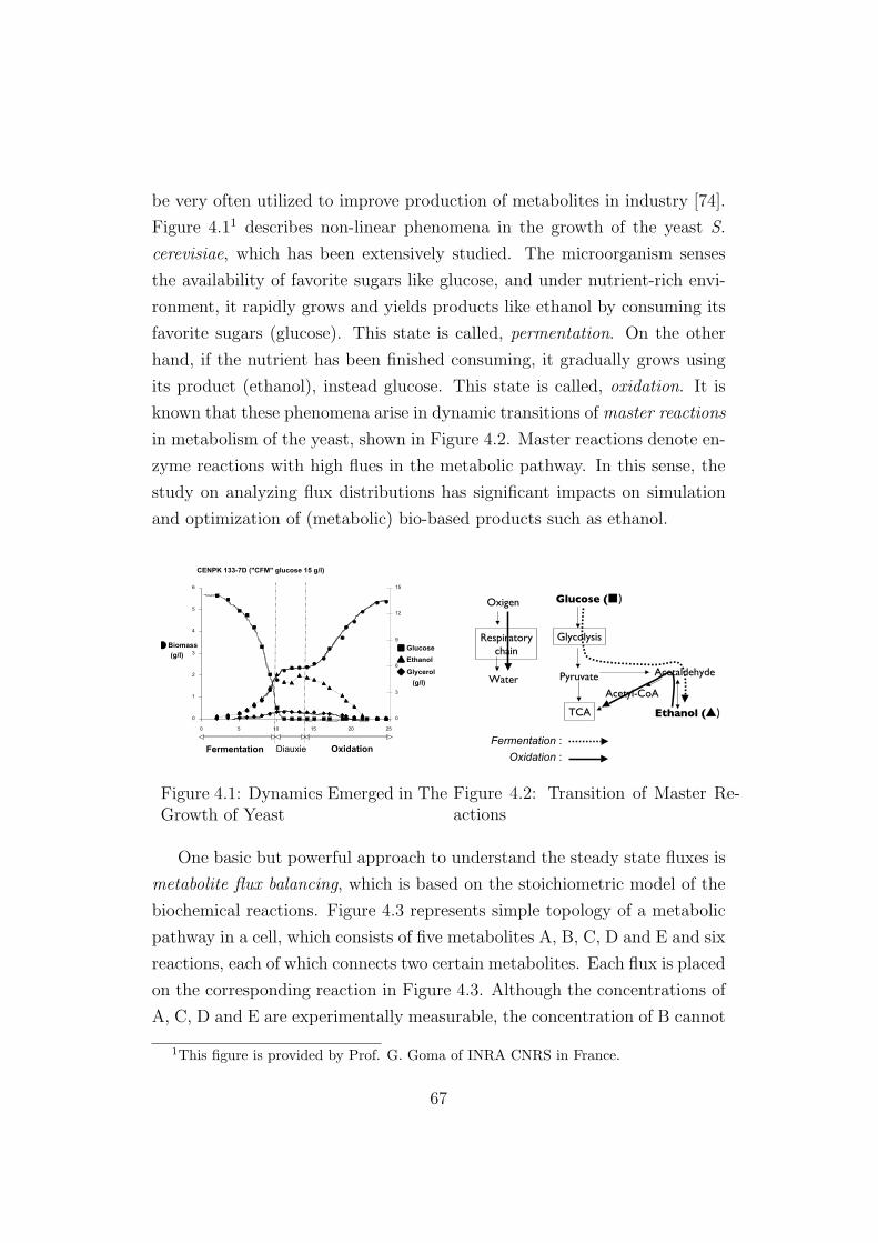
be very often utilized to improve production of metabolites in industry [74].
Figure 4.11 describes non-linear phenomena in the growth of the yeast S.
cerevisiae, which has been extensively studied. The microorganism senses
the availability of favorite sugars like glucose, and under nutrient-rich envi-
ronment, it rapidly grows and yields products like ethanol by consuming its
favorite sugars (glucose). This state is called, permentation. On the other
hand, if the nutrient has been finished consuming, it gradually grows using
its product (ethanol), instead glucose. This state is called, oxidation. It is
known that these phenomena arise in dynamic transitions of master reactions
in metabolism of the yeast, shown in Figure 4.2. Master reactions denote en-
zyme reactions with high flues in the metabolic pathway. In this sense, the
study on analyzing flux distributions has significant impacts on simulation
and optimization of (metabolic) bio-based products such as ethanol.
CENPK 133-7D ("CFM" glucose 15 g/l)
0
1
2
3
4
5
6
0 5 10 15 20 25
Temps (h)
● Biomass(g/l)
0
3
6
9
12
15
■ Glucose ▲ Ethanol
◆ Glycerol(g/l)
Fermentation Diauxie Oxidation
Figure 4.1: Dynamics Emerged in TheGrowth of Yeast
Glucose (Glucose (■)■)
GlycolysisGlycolysis
PyruvatePyruvate
Acetyl-Acetyl-CoACoA
TCATCA
AcetaldehydeAcetaldehyde
Ethanol (Ethanol (▲)▲)
OxigenOxigen
RespiratoryRespiratorychainchain
WaterWater
Fermentation : Oxidation :
Figure 4.2: Transition of Master Re-actions
One basic but powerful approach to understand the steady state fluxes is
metabolite flux balancing, which is based on the stoichiometric model of the
biochemical reactions. Figure 4.3 represents simple topology of a metabolic
pathway in a cell, which consists of five metabolites A, B, C, D and E and six
reactions, each of which connects two certain metabolites. Each flux is placed
on the corresponding reaction in Figure 4.3. Although the concentrations of
A, C, D and E are experimentally measurable, the concentration of B cannot
1This figure is provided by Prof. G. Goma of INRA CNRS in France.
67

E
Figure 4.3: System of Mass Balance
be measured. Hence, B is the intracellular metabolite. Based on the enzyme
kinetics, the dynamic behavior of the flux of an enzyme reaction can be
represented as the following differential equation:
dCX
dt= vin − vout − µCX , (4.1)
where CX is the concentration of a metabolite X, vin (resp. vout) is the
sum of fluxes of reactions for producing (resp. consuming) X, and µCX
represents the growth rate of biomass in a cell. If all the metabolites are
in the steady state, the left term of Equation (4.1) must be zero since there
are no time-series changes of the concentrations, and also, it can be assumed
that the dilution of components due to biomass growth (corresponding to the
last term of Equation (4.1)) is neglected [70]. This fact means that for each
metabolite X, the fluxes consuming X are balanced with the ones producing
X in the steady state. Metabolic flux balancing is based on this simple
notion. For example, its balancing in Figure 4.3 can be represented as the
following linear equations:
v1 = rA, rD + v5 = v2, rE + v4 = v5,
v2 + v3+ = v3− + v1, rC + v3− = v3+ + v4. (4.2)
Then we can analyze the flux distribution based on Equation (4.2) with the
measurable fluxes rA, rC, rD and rE. In general, these equations cannot be
deterministically solved as the number of unknown values such as v1, . . . , v5
corresponding to the fluxes of intracellular enzyme reactions becomes larger
than the number of known values corresponding to measurable fluxes. The
68
previously proposed methods such as elementary mode analysis and extreme
pathway analysis use optimization functions in order to solve the equations.
Those introduced functions are usually constructed by assuming the cellular
growth maximization or the energy consumption minimization. However,
these assumptions can often cause the dissociation with real situation. In
other words, we cannot necessarily determine if the organism indeed grows
based on the above assumptions to be expected. Additionally, in the case of
a large-scale of metabolic pathway, it is not straightforward to solve the flux
distribution with approximation methods due to huge computational cost.
In this work, we propose a new approach that enables us to release those
unsure assumptions and reduce the complexity of a given metabolic pathway.
One essential feature of enzymatic activities is that all the activities are
not necessarily on the same level. There exist enzymes whose activities are
about 100 or 1000 times higher than other enzymes. This fact allows us
to assume whether each enzyme reaction is in a relatively activated state or
not. Then, if we could estimate which enzyme reactions are in an activated
or a non-activated state, we could simplify the prior metabolic pathway by
ignoring those reactions in the non-activated state, which are estimated to
have low fluxes. The smaller the target pathway is, the smaller the number
of unknown values in the equations obtained from the pathway is. It may
imply that the possibility of solving the equations based on the metabolic
flux balancing without the previously proposed approximation methods. In
our approach, we introduce a logical model that represents causal relations
between enzyme reaction states and concentration changes of metabolites.
Based on the logical model, we can logically find possible states that can
explain the observations which are experimentally observed. In the following,
we focus on those causal relations in enzyme reactions.
4.2.2 Regulation of Enzymatic Activities
The cellular metabolic system has a sophisticated mechanism for dynamically
controlling the activities of enzymes to meet the needs of a cell. This regu-
latory mechanism can be represented as causal relations between enzymatic
69

activities and concentration changing of metabolites. Here we consider two
simple metabolic pathways: First one consists of two reactions with three
metabolites, and second one consists of one reaction with two metabolites.
Note that in the following figures, we describe activated and non-activated
reactions as (back) circles and slashes over arrows corresponding to reac-
tions, respectively. And also, a upward (resp. downward) arrow represents
the increase (resp. decrease) in a metabolite concentration.
Figure 4.4 corresponds to the metabolic pathway consisting of three metabo-
lites X, Y and Z, and two reactions. Figure 4.4 shows that if the concen-
Y X Z
Figure 4.4: First Biological Inference in Metabolic Pathways
tration of Y tends to be increasing at some time, provided that the state
of enzyme reaction Y → X (resp. X → Z) is in an activated (resp. non-
activated) state, then the concentration of X will also change to be increasing.
This causal relation is rational biological inference based on Equation (4.1).
Assume that the increase in concentration of X is observed, which is denoted
by a dotted arrow in the figures. Then, it will be possible to logically esti-
mate the states of the concentration change of Y and two reactions so that
the estimated states cause this concentration change of X. One possible case
is that the concentration of Y increases, the reaction Y → X is activated
and the reaction X → Z is not activated. This is because X produced from
Y cannot be consumed and generate Z.
Next, we consider Figure 4.5 which represents a metabolic pathway con-
sisting of two metabolites X and Y , and one reaction. Figure 4.5 shows that
Y X
Figure 4.5: Second Biological Inference in Metabolic Pathways
even if the reaction Y → X is activated, the concentration of X must de-
crease as far as the concentration of Y decreases. Accordingly, if we observe
70
the concentration of X decreases, we can logically estimate the concentration
of Y decreases and the reaction Y → X is activated as one possible case.
As we see in the above, consideration of these causal relations enables us
to estimate possible reaction states that explain the concentration changes
of measurable metabolites. Two causal relations shown in Figures 4.4 and
4.5 are not sufficient for explaining all the possible cases. In other words,
there exist cases that we cannot estimate possible reaction states using these
causal relations only. Although it would be possible to construct other causal
relations a priori, however it must be crucially difficult to enumerate all the
causal relations corresponding to the whole regulatory mechanism on enzy-
matic activities. This problem brings the necessity to complete the current
causal relations for estimation in some cases. Hence, we need to simultane-
ously realize these two tasks, that is, estimation of possible reaction states
and completion of missing causal relations.
We represent our problem in the ILP setting. The metabolic pathway
topology in Figure 4.3 can be represented as the following clausal theory T
consisting of facts:
T = {reac(a, b), reac(b, d), reac(d, e), reac(e, c), reac(b, c), reac(c, b)},
where the literal reac(X,Y ) means that there is a reaction between the sub-
strate X and the product Y . Along with the logical representation of topol-
ogy, we formalize the causal relations in Figures 4.4 and 4.5 as the following
two clauses (4.3) and (4.4), respectively:
reac(Y,X) ∧ reac(X,Z) ∧ con(Y, up)
∧ act(Y,X) ∧ ¬act(X,Z) ⊃ con(X, up), (4.3)
reac(Y,X) ∧ con(Y, down)
∧ act(Y,X) ⊃ con(X, down), (4.4)
where the literal con(X, up) (resp. con(X, down)) means that the concentra-
tion of the metabolite X increases (resp. decreases), and the literal act(X,Y )
means that the reaction X → Y is activated. Note that both (4.3) and (4.4)
are non-Horn clauses.
71
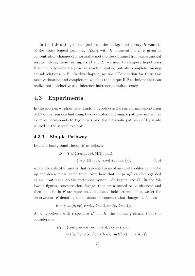
In the ILP setting of our problem, the background theory B consists
of the above logical formulas. Along with B, observations E is given as
concentration changes of measurable metabolites obtained from experimental
results. Using these two inputs B and E, we need to compute hypotheses
that not only estimate possible reaction states, but also complete missing
causal relations in B. In this chapter, we use CF-induction for these two
tasks estimation and completion, which is the unique ILP technique that can
realize both abductive and inference inference, simultaneously.
4.3 Experiments
In this section, we show what kinds of hypotheses the current implementation
of CF-induction can find using two examples. The simple pathway in the first
example corresponds to Figure 4.3, and the metabolic pathway of Pyruvate
is used in the second example.
4.3.1 Simple Pathway
Define a background theory B as follows:
B = T ∪ {con(a, up), (4.3), (4.4),
{¬con(X, up),¬con(X, down)}}, (4.5)
where the rule (4.5) means that concentrations of any metabolites cannot be
up and down at the same time. Note here that con(a, up) can be regarded
as an input signal to the metabolic system. So is put into B. In the fol-
lowing figures, concentration changes that are assumed to be observed and
then included in E are represented as dotted bold arrows. Thus, we let the
observations E denoting the measurable concentration changes as follows:
E = {con(d, up), con(c, down), con(e, down)}.
As a hypothesis with respect to B and E, the following clausal theory is
considerable:
H1 = {con(e, down) ← ¬act(d, e) ∧ act(e, c),
act(a, b), act(e, c), act(b, d),¬act(b, c),¬act(d, e)}.
72

A B
C
D
E
Figure 4.6: First Hypothesis H1
A B
C
D
E
Figure 4.7: Second Hypothesis H2
Figure 4.6 shows the reaction states in H1. According to H1, whereas the
reactions A → B, B → D and E → C are activated, the reactions B → C
and D → E are not activated. This estimation of reaction states is realized
using abduction. On the other hand, we cannot explain the reason why the
concentration of E decreases only with abductive hypotheses. For explaining
this concentration decreasing of E, H1 includes a new rule worth considering
as a reasonable answer, that is, “the concentration of E decreases if the
reaction D → E is not activated and the reaction E → C is activated”.
As another hypothesis, the following clausal theory can be also considered:
H2 = {con(X, down) ← ¬act(Y,X) ∧ con(Y, up),
act(a, b), act(b, d),¬act(b, c),¬act(d, e)}.
Figure 4.7 shows the states of reactions in H2. Compared with H1, the rule
for explaining the concentration change of E is more general, and also H2
does not say whether the reaction E − C is activated or not. Hence, the
hypothesis H2 logically estimates several reaction states and completes one
missing rule on biological inference in metabolic pathways.
These two hypotheses can be indeed computed using the implementation
of CF-induction. Let a production field P be as follows:
P = 〈{con(X,Y ),¬con(X,Y ),¬act(X,Y ), act(X,Y )}〉.
Note that, due to computational efficiency, we set the maximum length
of characteristic clauses and the maximum search-depth for computing the
characteristic clauses as 6 and 4, respectively. Then, CF-induction displays
73
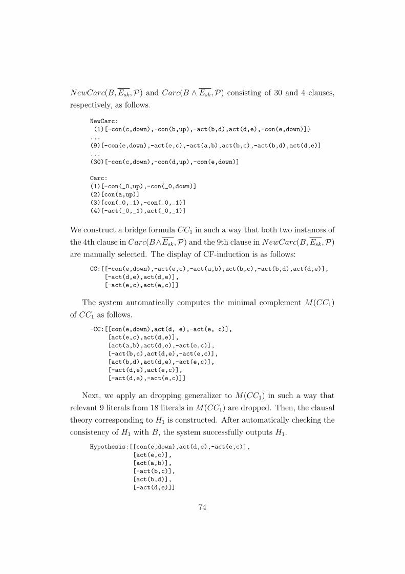
NewCarc(B, Esk,P) and Carc(B ∧ Esk,P) consisting of 30 and 4 clauses,
respectively, as follows.
NewCarc:(1)[-con(c,down),-con(b,up),-act(b,d),act(d,e),-con(e,down)]}...(9)[-con(e,down),-act(e,c),-act(a,b),act(b,c),-act(b,d),act(d,e)]...(30)[-con(c,down),-con(d,up),-con(e,down)]
Carc:(1)[-con(_0,up),-con(_0,down)](2)[con(a,up)](3)[con(_0,_1),-con(_0,_1)](4)[-act(_0,_1),act(_0,_1)]
We construct a bridge formula CC1 in such a way that both two instances of
the 4th clause in Carc(B∧Esk,P) and the 9th clause in NewCarc(B, Esk,P)
are manually selected. The display of CF-induction is as follows:
CC:[[-con(e,down),-act(e,c),-act(a,b),act(b,c),-act(b,d),act(d,e)],[-act(d,e),act(d,e)],[-act(e,c),act(e,c)]]
The system automatically computes the minimal complement M(CC1)
of CC1 as follows.
-CC:[[con(e,down),act(d, e),-act(e, c)],[act(e,c),act(d,e)],[act(a,b),act(d,e),-act(e,c)],[-act(b,c),act(d,e),-act(e,c)],[act(b,d),act(d,e),-act(e,c)],[-act(d,e),act(e,c)],[-act(d,e),-act(e,c)]]
Next, we apply an dropping generalizer to M(CC1) in such a way that
relevant 9 literals from 18 literals in M(CC1) are dropped. Then, the clausal
theory corresponding to H1 is constructed. After automatically checking the
consistency of H1 with B, the system successfully outputs H1.
Hypothesis:[[con(e,down),act(d,e),-act(e,c)],[act(e,c)],[act(a,b)],[-act(b,c)],[act(b,d)],[-act(d,e)]]
74

Test (depth = 6, max length = 6)example con(c, down) con(d, up) con(e, down)
NH 21 22 22NP 8 2 7
Ratio [%] 38 9 32Time [msec] 6915 11360 10751
Table 4.1: Performance of abductive explanations in CF-induction
Next, we set the maximum length of characteristic clauses and the maxi-
mum search-depth for computing the characteristic clauses as 6 and 6. Then,
NewCarc(B, Esk,P) (resp. Carc(B ∧ Esk,P)) increases to 137 (resp. 84)
clauses. We construct another bridge formula CC2 in such a way that one
clause in NewCarc(B, Esk,P), two clauses and two instances of a clause in
Carc(B ∧ Esk,P) are selected. After computing the minimal complement
M(CC2) of CC2 , we apply both a dropping and an anti-instantiation gener-
alizers to M(CC2) in such a way that relevant 15 literals are dropped from
27 literals in M(CC2) and 4 constants are replaced by variables. Then, the
clausal theory corresponding to H2 is constructed.
Both H1 and H2 need inductive inference to be constructed. It becomes
necessary to apply inductive inference for completing missing general rules.
Another role of inductive inference is to find such hypotheses that have high
predictive accuracy to unknown observations, which are generated by apply-
ing generalizers like anti-instantiation. Indeed, if abductive inference is only
used, the predicate accuracy tend to become low, as we describe in the below.
Table 4.1 shows the predicate accuracy of abductive hypotheses each of
which is a set of ground unit clauses, such as {act(a, b), ¬act(b, c)}, ob-
tained by CF-induction. Since the negation of every abductive hypothesis is
the form of ground clause, every subsumption-minimal abductive hypothe-
sis can be derived by CF-induction in such a way that a bridge theory CC
only contains one ground instance of a clause in NewCarc(B, Esk,P), and
outputs the minimal complement M(CC) without applying any generalizers
[26]. We then evaluated the predictive accuracy of those minimal abductive
hypotheses using a leave-one-out strategy [5].
75

First, we select one clause C in observations E as a test example. Second,
for each new characteristic clause D in NewCarc(B, E − {C},P), we check
whether or not the minimal abductive hypothesis M({D}) derives the test
example C with respect to B, that is, B ∧ M({D}) |= {C}. In case of
the simply pathway problem, we assume E is ground, and thus every new
characteristic clause in NewCarc(B, E − {C},P) is also ground.
NH and NP in Table 4.1 denote the number of minimal abductive hy-
potheses with respect to B, E − {C} and P and the number of those hy-
potheses that can also explain the test example C. This experimental result
shows that CF-induction can generate abductive hypotheses such that accu-
rately predict each (unseen) test example. However, we may notice that the
ratio of NP to NH is not so high. It means that though several abductive
hypotheses succeeded with the prediction of a unseen test example, most of
them could not do. This fact shows the necessity of not only abductive but
also inductive inference to improve the predictive accuracy of hypotheses.
4.3.2 Metabolic Pathway of Pyruvate
Next, we consider the metabolic pathway of Pyruvate (see Figure 4.8). The
logical representation of topology in Figure 4.8 is as follows:
T ′ = {terminal(ethanol), reac(pyruvate, acetylcoa),
reac(pyruvate, acetaldehyde), reac(glucose, glucosep),
reac(glucosep, pyruvate), reac(acetaldehyde, acetate),
reac(acetate, acetylcoa), reac(acetaldehyde, ethanol)},
where the predicate terminal(X) means that there is no reaction where X
is consumed. If the metabolite X is terminated and there is activated reac-
tion that produces X, then the concentration of X must increase. However,
this consequence cannot be derived only using the previous causal rule (4.3)
which concerns with the concentration increase of a metabolite. Thus, we
construct the following new causal rules obtained by incorporating the con-
76

Acetate
AcetaldehydePyruvate
Glucose-P
Ethanol
Glucose
Acetylcoa
Figure 4.8: Metabolic Pathway of Pyruvate
cept of “terminal” with the rule (4.3):
reac(X,Z) ∧ ¬act(X,Z) ⊃ blocked(X), (4.6)
terminal(X) ⊃ blocked(X), (4.7)
reac(Y,X) ∧ act(Y,X) ∧ blocked(X) ⊃ con(X, up), (4.8)
where the predicate blocked(X) means that the metabolite X cannot be
consumed, and the predicate terminal(X) means that the metabolite X is
terminated. Define a background theory B as follows:
B = T ′ ∪ {(4.6), (4.7), (4.8), con(glucose, up)}.
Next, we input the following observations E:
E = {con(ethanol, up), con(pyruvate, up)}.
Then, the following clausal theories H3 and H4 are considerable as hypotheses
with respect to B and E.
H3 = {act(glucosep, pyruvate),
¬act(pyruvate, acetylcoa), act(acetaldehyde, ethanol)}.
H4 = {act(X,Y ) ∧ con(X, up) ⊃ con(Y, up),
act(glucosep, pyruvate), act(acetaldehyde, ethanol),
act(pyruvate, acetaldehyde), act(glucose, glucosep)}.
Figure 4.9 and 4.10 show the states of reactions in H3 and H4, respectively.
Compared with H3, H4 includes a new general rule concerning the mecha-
nism of how concentrations of metabolites increase. Both H3 and H4 can be
77

Acetate
AcetaldehydePyruvate
Glucose-P
Ethanol
Glucose
Acetylcoa
Figure 4.9: Third Hypothesis H3
Acetate
AcetaldehydePyruvate
Glucose-P
Ethanol
Glucose
Acetylcoa
Figure 4.10: Forth Hypothesis H4
generated using CF-induction. Let a production field P be as follows:
P = 〈{con(X,Y ),¬con(X,Y ),¬act(X,Y ), act(X,Y )}〉.
We set the maximum length of characteristic clauses and the maximum
search-depth as 6 and 4, respectively. Then, CF-induction displays the fol-
lowing NewCarc(B, Esk,P) and Carc(B ∧Esk,P), which consist of 6 and 3
clauses, respectively.
NewCarc:(1)[-act(acetaldehyde,ethanol),-con(pyruvate,up)](2)[-con(ethanol,up),-act(glucosep,pyruvate),
act(pyruvate,acetylcoa)](3)[-con(ethanol,up),-act(glucosep,pyruvate),
act(pyruvate,acetaldehyde)](4)[-act(acetaldehyde,ethanol),-act(glucosep,pyruvate),
act(pyruvate,acetylcoa)](5)[-act(acetaldehyde,ethanol),-act(glucosep,pyruvate),
act(pyruvate,acetaldehyde)](6)[-con(ethanol,up),-con(pyruvate,up)]
Carc:(1)[con(glucose,up)](2)[-act(_0,_1),act(_0,_1)](3)[con(_0,_1),-con(_0,_1)]
We first manually construct the bridge theory CC3 which contains only the
4th clause in NewCarc(B, Esk,P). The system automatically computes
the minimal complement of CC3, which corresponds to H3. Note that no
generalizer is necessary to generate H3. We next construct the bridge for-
mula CC4 for finding H4 which contains the two 1st and 5th clauses in
NewCarc(B, Esk,P) and the 1st clause, four instances of the 2nd clause
78

and one instance of the 3rd clause in Carc(B ∧ E,P). Note that CC4 to-
tally contains 8 clauses. After computing the minimal complement of CC4,
CF-induction outputs H4 using both a dropping and an anti-instantiation
generalizers.
4.4 Related Work
Tamaddoni-Nezhad et al. studied estimation of inhibitory effects on metabolic
pathways using ILP [76]. Inhibition of enzyme functions plays an impor-
tant role on dynamically controlling enzymatic activities on metabolism.
They have also introduced the logical modeling of metabolic pathways and
firstly showed the possibility of application of ILP to qualitatively analyzing
metabolic pathways with their logical model on inhibitory effects to con-
centration changes of metabolites. Here, we refer to three points as the
difference, compared with their work.
The first point is the difference of main goal that we try to solve using
ILP techniques. Our long-term goal is more precise modeling of the flux
distribution corresponding to dynamics on enzymatic activities. Previously
proposed techniques in MFA that quantitatively analyzes the flux distribu-
tion can have several limitations involved in embedded approximation con-
ditions as well as computational costs in the case of large-scale of metabolic
pathways. Using ILP techniques, we can logically estimate possible reaction
states in metabolic pathways, which enable us to reconstruct the prior path-
way into more simplified one by removing enzyme reactions with low fluxes.
In other words, we intend to reduce the complexity of metabolic pathways.
In contrast, they have focused on the inhibitory effects of particular toxins
affected to objects to be examined, which are used as drugs.
The second point is the difference of ILP techniques applied to problems.
They have used Progol5.0 [46] that is one of the successful ILP systems and
can also compute both inductive and abductive hypotheses. Compared with
Progol5.0, CF-induction preserves the soundness and completeness for find-
ing hypotheses and can use not only Horn but also non-Horn clauses in the
knowledge representation formalisms. In [76], they have evaluated the pre-
79

dictive accuracy of both abductive and inductive hypotheses obtained by
Progol5.0 in the metabolic pathway consisting of 76 enzyme reactions and
31 metabolites. The data set of this metabolic pathway is available on their
website. Then, it will be interesting that we evaluate the hypotheses obtained
by CF-induction using the data set. Note that in an initial experiment with
this data set, CF-induction computes 66 (subsumption-minimal) abductive
hypotheses including the unique output of Progol5.0 when we set the maxi-
mum search-depth as 5 and put the maximum length of a production field as
15. The following example is concerning with an inductive hypothesis intro-
duced in [76]. We show how CF-induction can compute the same inductive
hypothesis as the one obtained by Progol5.0 using the next example.
Example 4.1. Define a background theory B and an observation E as fol-
lows:
B = {reac(X,Y, Z) ∧ inh(X,Y, Z) ⊃ con(X, up),
reac(s, e, p), class(e, c)},
E = con(s, up).
The predicate reac(X,Y, Z) includes the new term Y which denotes an en-
zyme catalyzing the reaction X → Z. The predicate inh(X,Y, Z) means the
reaction between a substrate X and a product Z, catalyzed by an enzyme Y ,
is inhibited. Note that those reactions that are inhibited might be regarded
as non-activated reactions. However, the activated state does not necessar-
ily always correspond to the non-inhibited state. Because there are other
factors expects for inhibition, which make enzyme reactions inactivated. We
thus need to distinguish the “inhibited” state with the “non-activated” state.
Along with the predicate inh(X,Y, Z), the predicate class(X,Y ) is newly in-
troduced. It means that an enzyme X belongs to an enzyme class Y . In [76],
the following inductive hypothesis H is introduced:
H = inh(s,X, p) ← class(X, c).
This hypothesis can be derived by CF-induction. Suppose the following
production field P :
P = 〈{inh(X,Y, Z),¬inh(X,Y, Z), class(X,Y )}〉.
80

B: con(X, up) ← reac(X,Y, Z) ∧ inh(X,Y, Z), reac(s, e, p), class(e, c)
E: con(s, up)
(abduction) inh(s, e, p)
(induction) inh(s,X, p) ← class(X, c)
Figure 4.11: Integrating Abduction and Induction for Finding Hypotheses
NewCarc(B, Esk,P) and Carc(B ∧ Esk,P) are computed as follows:
NewCarc(B, Esk,P) = {¬inh(s, e, p),¬con(s, up)},
Carc(B ∧ Esk,P) = {class(e, c),¬inh(s, e, p)}.
Let a bridge formula CC be the clausal theory {¬inh(s, e, p), class(e, c)}.Then, the minimal complement of CC is as follows:
M(CC) = inh(s, e, p) ← class(e, c).
If we apply an anti-instantiation generalizer to M(CC) in such a way that
the ground term e appearing in F is replaced with the variable X, then the
hypothesis H can be generated.
The process of computing the above inductive hypothesis can be sketched
in Figure 4.11. An inductive hypothesis is constructed based on a certain
abductive explanation. Hence, it is necessary to generate abductive hypothe-
ses in advance for constructing inductive hypotheses. Indeed, Progol5.0 first
computes an abductive hypothesis, and second find inductive hypotheses us-
ing the abductive explanation. In other words, Progol5.0 performs abduction
and induction processes, step by step. On the other hand, CF-induction can
realize them with one process. This difference of those mechanisms for inte-
grating abduction and induction is the last and crucial point. In our problem
setting, we need to not only estimate possible reaction states but also com-
plete missing general rules in the prior background. CF-induction can realize
these two tasks simultaneously using both abduction and induction.
There are several works that have studied on applications of ILP tech-
niques to biology [32, 94], as we described in Chapter 1. King et al. showed
81
that hypothesis finding techniques can help to reduce the experimental costs
for predicting the functions of genes in their project, called robot sceientist
[32]. Besides, Zupan et al. have developed a system based on abduction,
which enables us to find new relations from experimental genetic data for
completing the prior genetic networks [94].
4.5 Summary
We have studied a logic-based method for estimating possible states of en-
zyme reactions. Since this method can help us to understand which enzyme
reactions are activated, it can be potentially used in MFA, in that it is impor-
tant for optimization or improvement of production and to identify master
reactions that have high fluxes. In this work, we have showed how CF-
induction can realize not only estimation of possible reaction states, but also
completion of the current causal relations.
On the other hand, it is still far from our long-term goal that we construct
a new technique integrating our logic-based analysis with previously proposed
MFA methods. As an important remark, we point out the issue on com-
pleteness and non-determinism in hypothesis fining techniques. Systems like
Progol can deterministically generate a hypothesis. However, since it does
not ensure completeness in hypothesis finding, some important hypotheses
might fail to be generated. In contrast, CF-induction ensures the complete-
ness, and thus can achieve such an advanced inference that simultaneously
integrates abduction and induction. However, since CF-induction consists
of several highly non-deterministic procedures, it is not straightforward to
apply to practical problems that have to deal with a huge number of data.
In next chapter, we treat this issue and investigate how the non-determinism
in generalization of IE-based ILP methods can be logically reduced.
82

Chapter 5
From Inverse Entailment toInverse Subsumption
As we explained in Chapter 3, modern explanatory ILP methods like Pro-
gol, Residue procedure, CF-induction, HAIL and Imparo use the principle of
Inverse Entailment (IE). It is based on the fact that the negation of a hypoth-
esis is derived from a prior background theory and the negation of examples.
IE-based methods commonly compute a hypothesis in two steps: by first con-
structing an intermediate theory and next by generalizing its negation into
the hypothesis with the inverse relation of entailment. In this chapter, we
focus on the sequence of intermediate theories that constructs a derivation
from the background theory and the negation of examples to the negation of
the hypothesis. We then show the negations of those derived theories in a
sequence are represented with inverse subsumption. Using our result, inverse
entailment can be reduced into inverse subsumption, while it preserves the
completeness for finding hypotheses.
5.1 Introduction
Given a background theory B and observations E, the task of explanatory
induction is to find a hypothesis H such that B ∧ H |= E and B ∧ H
is consistent [26]. By the principle of Inverse Entailment (IE) [44], this
is logically equivalent to finding a consistent hypothesis H such that B ∧¬E |= ¬H. This equivalence means that the inductive hypothesis H can be
83

computed by deducing its negation ¬H from B and ¬E. We represent this
derivation process as follows:
B ∧ ¬E |= F1 |= · · · |= Fi |= · · · |= Fn |= ¬H (5.1)
where each Fi (1 ≤ i ≤ n) denotes a clausal theory. IE-based methods
[26, 31, 44, 61, 63, 75, 83] compute a hypothesis H in two ways: by first
constructing an intermediate theory Fi in Formula (5.1) and next generalizing
its negation ¬Fi into the hypothesis H with the inverse relation of entailment.
The logical relation between ¬Fi and H is obtained from the contrapositive
of Formula (5.1) as follows:
¬(B ∧ ¬E) =| ¬F1 =| · · · =| ¬Fi =| · · · =| ¬Fn =| H (5.2)
where =| denotes the inverse relation of entailment. Hereafter, we call it the
generalization relation. In brief, IE-based methods first use the entailment
relation to construct Fi with Formula (5.1), and then switch to the general-
ization relation to generate the hypothesis H with Formula (5.2) (See Figure
5.1).
@@ -B ∧ ¬E |= F1 |= · · · |= Fi (Generalization relation)¬Fi =| · · · =| ¬Fn =| H
Figure 5.1: Hypothesis Finding Based on Inverse Entailment
The inverse relation of entailment ensures the completeness in finding hy-
potheses from an intermediate theory by Formula (5.2). However, the gener-
alization procedures with this relation need a variety of different generalizers,
such as dropping and inverse resolution [47]. As shown in Chapter 3, there
are several such operators and each one can be applied in many different
ways, which lead to a large number of choice points. For this reason, systems
like Progol [44, 75] and HAIL [61, 63] use subsumption due to computational
efficiency, though their generalization procedures may become incomplete.
On the other hand, systems like CF-induction [26] use entailment to find any
hypothesis, though they need to handle a huge search space.
In this chapter, we show inverse subsumption is an alternative generaliza-
tion relation to ensure the completeness for finding hypotheses (See Figure
5.2).
84
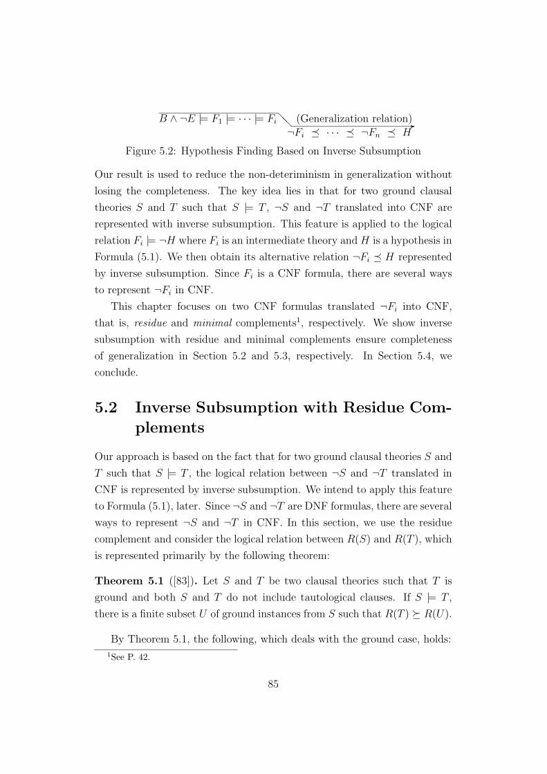
@@ -B ∧ ¬E |= F1 |= · · · |= Fi (Generalization relation)¬Fi ¹ · · · ¹ ¬Fn ¹ H
Figure 5.2: Hypothesis Finding Based on Inverse Subsumption
Our result is used to reduce the non-deteriminism in generalization without
losing the completeness. The key idea lies in that for two ground clausal
theories S and T such that S |= T , ¬S and ¬T translated into CNF are
represented with inverse subsumption. This feature is applied to the logical
relation Fi |= ¬H where Fi is an intermediate theory and H is a hypothesis in
Formula (5.1). We then obtain its alternative relation ¬Fi ¹ H represented
by inverse subsumption. Since Fi is a CNF formula, there are several ways
to represent ¬Fi in CNF.
This chapter focuses on two CNF formulas translated ¬Fi into CNF,
that is, residue and minimal complements1, respectively. We show inverse
subsumption with residue and minimal complements ensure completeness
of generalization in Section 5.2 and 5.3, respectively. In Section 5.4, we
conclude.
5.2 Inverse Subsumption with Residue Com-
plements
Our approach is based on the fact that for two ground clausal theories S and
T such that S |= T , the logical relation between ¬S and ¬T translated in
CNF is represented by inverse subsumption. We intend to apply this feature
to Formula (5.1), later. Since ¬S and ¬T are DNF formulas, there are several
ways to represent ¬S and ¬T in CNF. In this section, we use the residue
complement and consider the logical relation between R(S) and R(T ), which
is represented primarily by the following theorem:
Theorem 5.1 ([83]). Let S and T be two clausal theories such that T is
ground and both S and T do not include tautological clauses. If S |= T ,
there is a finite subset U of ground instances from S such that R(T ) º R(U).
By Theorem 5.1, the following, which deals with the ground case, holds:
1See P. 42.
85

Proposition 5.1 ([90]). Let S and T be two ground clausal theories such
that S and T do not include tautological clauses. If S |= T , then R(T ) ºR(S).
We first recall the following lemma to prove Proposition 5.1.
Lemma 5.1 ([83]). For ground clausal theories S and T that do not include
tautological clauses, T ⊂ S implies R(T ) º R(S).
Using Lemma 5.1 as well as Theorem 5.1, Proposition 5.1 is proved:
Proof. By Theorem 5.1, there is a ground theory U such that U ⊆ S such that
R(T ) º R(U). By Lemma 5.1, R(U) º R(S) holds. Hence, R(T ) º R(S)
holds. 2
We apply this proposition to the logical relation F |= ¬H where F is a
bridge theory2 and H is a ground hypothesis. We represent ¬H using the
residue complement R(H). Suppose that F does not include any tautological
clauses. Then, by Propositon 5.1, R2(H) º R(F ) holds. In other words,
R2(H), which is logically equivalent to H, can be obtained from R(F ) using
inverse subsumption. This property is described as the following theorem:
Theorem 5.2 ([90]). Let F be a bridge theory such that F do not include
tautological clauses, and H a hypothesis such that F |= ¬H. Then, there is
a hypothesis H∗ such that H∗ ≡ H and H∗ º R(F ).
Proof. By Herbrand theorem, there is a ground clausal theory Hg such that
H º Hg and F |= ¬Hg. Since ¬Hg ≡ R(Hg) holds, R2(Hg) º R(F ) holds
by Proposition 5.1. Assume the clausal theory H∗ = H ∪ R2(Hg). Since
H º Hg and Hg ≡ R2(Hg), H |= R2(Hg) holds. Accordingly, H |= H∗ holds.
Hence, H∗ ≡ H holds. Since R2(Hg) º R(F ) and H∗ ⊇ R2(Hg), H∗ º R(F )
holds. 2
However, every target hypothesis is not necessarily obtained from the residue
complement by inverse subsumption, as described in the below examples.
2We refer to P.46 for the formal definition of bridge theories.
86

Example 5.1. Let B, E and H be a background theory, observations and
a target hypothesis as follows:
B = {p(a)}. E = {p(f(f(a))}.
H = {{p(a) ⊃ p(f(a)), p(f(a)) ⊃ p(f(f(a)))}}.
Let F be the clausal theory {p(a),¬p(f(f(a)))}. Since F = B ∪ ¬E, F
is a bridge theory wrt B and E such that F |= ¬H. R(F ) is {p(a) ⊃p(f(f(a)))}. Then we notice that R(F ) is not subsumed by H. Indeed,
R(F ) is the resolvent of two clauses in H. Then, we may need to apply an
inverse resolution operator to R(F ) for obtaining the target hypothesis H.
Example 5.2. We recall Example 3.3 in Chapter 3 as follows:
B = {arc(a, b), arc(X,Y ) ∧ path(Y, Z) ⊃ path(X,Z)}.
E = {path(a, c)}.
H = {arc(b, c), arc(X,Y ) ⊃ path(X,Y )}.
Let F be the clausal theory as follows:
F = {arc(a, b), arc(a, b) ∧ path(b, c) ⊃ path(a, c), ¬path(a, c)}.
Since F is the set of ground instances from B∧¬E, F is a bridge theory wrt
B and E. Assume the following ground hypothesis Hg consisting of ground
instances of H:
Hg = {arc(b, c), arc(X,Y ) ⊃ path(X,Y )}.
Since F ∧Hg is inconsistent, F satisfies the condition of Theorem 5.2. Hence,
there is a hypothesis H∗ such that H∗ ≡ H and H∗ º R(F ). F and R(F )
are as follows:
F = {{¬arc(a, b), arc(a, b), path(a, c)},
{¬arc(a, b), path(b, c), path(a, c)},
{¬arc(a, b), ¬path(a, c), path(a, c)}}.
R(F ) = {{¬arc(a, b), path(b, c), path(a, c)}}
87
We then consider the following clausal theory as H∗:
H∗ = H ∪ {path(b, c)}.
H∗ is equivalent to H, since the added clause C = {path(b, c)} can be derived
from H. We may notice that C subsumes the clause in R(F ). Then, H∗ ºR(F ) holds. Hence, there is in fact a hypothesis H∗ such that H∗ ≡ H
and H∗ º R(F ). However, the target hypothesis H itself does not subsume
R(F ). Instead, we may notice that the clause C is a resolvent of two clauses
in H. Then, it is necessary to use an inverse resolution operator for obtaining
the target hypothesis H.
This problem is caused by the fact that R2(H) = H cannot necessarily
hold for a ground clausal theory H. The key idea in Theorem 5.2 lies in
the logical relation R2(H) º R(F ). Hence, if R2(H) = H should not hold,
H cannot be obtained from R(F ) using inverse subsumption. We thus need
some CNF formula F (H) for representing the negation of a hypothesis H
such that F (F (H)) = H.
5.3 Inverse Subsumption with Minimal Com-
plements
We here investigate an alternative generalization using minimal complements.
We first show a key property that minimal complements satisfy.
5.3.1 Fixed-Point Theorem on Minimal Complements
Theorem 5.3 ([89]). Let S be a ground clausal theory. Then M2(S) = µS
holds.
Proof. By Theorem 2.5, M2(S) = MHS2(S) holds. By Lemma 5.2, it holds
that MHS2(S) = µS. Hence, M2(S) = µS holds. 2
The above proof uses the below lemma as well as Theorem 2.4 and Theo-
rem 2.5, which concerned a property on minimal hitting sets and a relation
between minimal hitting sets and minimal complements, respectively.
88
Lemma 5.2 ([89]). Let S be a ground clausal theory. Then MHS2(S) = µS
holds.
(Proof of µS ⊆ MHS2(S).)
We show every clause in µS is a minimal hitting set of F(MHS(S)). By
the definition of MHS(S), for every clause D ∈ MHS(S), D satisfies that
D ∩ C 6= ∅ for every set C ∈ F(S). In other words, for every set C ∈F(S), C satisfies that D ∩ C 6= ∅ for every clause D ∈ MHS(S). Then
every set C ∈ F(S) is a hitting set of MHS(S). Let C ′ be the set of
negations of literals in C. Since C ∈ F(S), C ′ ∈ F(F(S)) holds. Since C is
a hitting set of MHS(S), C ′ is a hitting set of F(MHS(S)). Accordingly,
every set C ∈ F(F(S)) is a hitting set of F(MHS(S)). Since the family
F(F(S)) corresponds to S, it holds that every clause C ∈ S is a hitting
set of F(MHS(S)). Since µS ⊆ S, every clause C ∈ µS is a hitting set of
F(MHS(S)).
Suppose that there is a clause C ∈ µS such that C is not a minimal
hitting set of F(MHS(S)). Then
(*) there is a literal l ∈ C such that C −{l} is a hitting set of F(MHS(S)).
For every clause Ci ∈ µS, if Ci 6= C then there is a literal li ∈ Ci such that
li 6∈ C. We then consider those literals E = {l1, l2, . . . , ln}, where each li
is a literal of Ci ∈ µS − {C} such that li is not included in C. Note that
E∩C = ∅ holds. On the other hand, for any literal l ∈ C, the intersection of
E ∪{l} and each clause in µS is not empty. Hence, E ∪{l} is a hitting set of
µS. Accordingly, E ∪ {l} is also a hitting set of S. Then there is a minimal
hitting set E ′ ∈ F(MHS(S)) such that E ′ ⊆ E ∪ {l}. Since E ′ ⊆ E ∪ {l}and E ∩ C = ∅, it holds that E ′ ∩ (C − {l}) = ∅. However, this contradicts
that C − {l} is a hitting set of F(MHS(S)) since E ′ ∈ F(MHS(S)). Then
the assumption (*) is false. Hence, every clause C in µS is a minimal hitting
set of F(MHS(S)). In other words, for every C ∈ µS, C ∈ MHS2(S) holds.
(Proof of MHS2(S) ⊆ µS.)
Let D be a clause in MHS2(S). Suppose that there is a clause C ∈ µS such
89

that C ⊂ D. Since µS ⊆ MHS2(S), C ∈ MHS2(S) holds. This contradicts
with the minimality of MHS2(S). Hence, for every clause C ∈ µS, C 6⊂ D.
In other words, for ever clause C ∈ µS, C = D or C 6⊆ D. Suppose that
(*) for any clause C ∈ µS, C 6= D holds.
Then, C 6⊆ D holds. Accordingly, for every clause Ci ∈ µS, there is a literal
li ∈ Ci such that li 6∈ D. We consider the finite set E = {l1, l2, . . . , ln} where
each literal li corresponds to such the above literal that is not included in D.
Note that E∩D = ∅. On the other hand, the intersection of E and each clause
in µS is not empty. Hence, E is a hitting set of µS. Accordingly, E is a hitting
set of S. Then, there is a minimal hitting set E ′ of S such that E ′ ⊆ E.
Since MHS(S) is the set of minimal hitting sets of F(S), F(MHS(S))
corresponds to the set of minimal hitting sets of F(F(S)). Since F(F(S)) =
S, F(MHS(S)) is the set of minimal hitting sets of S. Hence, we have
E ′ ∈ F(MHS(S)). Since E ′ ⊆ E and E ∩ D = ∅, E ′ ∩ D = ∅ holds. Note
here that since D ∈ MHS2(S), D is a minimal hitting set of F(MHS(S)).
However this contradicts that there is the set E ′ ∈ F(MHS(S)) such that
E ′ ∩ D = ∅. Then the assumption (*) is false. Hence, there is a clause
C ∈ µS such that C = D. Therefore, D ∈ µS holds. 2
Theorem 5.3 can be regarded as a fixed-point theorem on the function M
computing the minimal complement. Unlike residue complements, M2(S)
corresponds with S in case that S is subsume-minimal. Thus, minimal
complements may not cause the problem in residue complements that they
cannot necessarily obtain a target hypothesis using inverse subsumption, as
described in Section 5.3.
Example 5.3. Let S be the clausal theory {a∨b, b∨c, ¬c}. Then, S, R(S),
R2(S), M(S) and M2(S) are as follows. In fact, M2(S) = S holds, whereas
90

R2(S) does not. Note that M(S) contains a tautological clause.
S = {¬a ∨ ¬b ∨ c, ¬a ∨ ¬c ∨ c, ¬b ∨ c, ¬b ∨ ¬c ∨ c}.
R(S) = {¬a ∨ ¬b ∨ c, ¬b ∨ c}. R2(S) = {a ∨ b, ¬c ∨ a, b, ¬c ∨ b, ¬c}.
M(S) = {¬a ∨ ¬c ∨ c, ¬b ∨ c}. M2(S) = {a ∨ b, b ∨ c, ¬c}.
On the other hand, minimal complements do not necessarily satisfy the
logical relation that M(T ) º M(S) for ground clausal theories S and T such
that S |= T . We recall Example 5.1. Whereas F |= M(H) holds, M2(H),
which is equal to H by Theorem 5.3, does not subsume M(F ). This is
because minimal complements can include tautological clauses that residue
complements never have. Indeed, Proposition 5.1, which shows the logical
relation between R(T ) and R(S), does not allow tautological clauses to be
included in S and T . In next subsection, we extend Proposition 5.1 so as to
deal with tautological clauses.
5.3.2 Inverting Deductive Operations with Tautologies
Theorem 5.4 ([90]). Let S and T be ground clausal theories such that
S |= T and for every tautological clause D ∈ T , there is a clause C ∈ S such
that C º D. Then, τM(T ) º τM(S). holds.
We use the following deductive operators for proving this theorem:
Definition 5.1 (Deductive operators [83]). Let S and T be clausal theories.
Then T is directly-derivable from S if T is obtained from S by one of the
following three operators:
1. (resolution) T = S∪{C}, where C is a resolvent of two clauses D1, D2 ∈S.
2. (subsumption) T = S ∪ {C}, where C is subsumed by some clause
D ∈ S.
3. (weakening) T = S − {D} for some clause D ∈ S.
91
We write S `r T , S `s T , S `w T to denote that T is directly derivable from S
by resolution, subsumption, weakening, respectively. `∗X is the reflexive and
transitive closure of `X , where X is one of the symbols r, s, w. Alternatively,
S `∗X T if T follows from S by application of zero or more `X .
We now show that entailment between theories can be established by
applying these operators in a particular order.
Theorem 5.5 ([92]). Let S be a clausal theory and T be a clausal theory
without any tautological clauses. If S |= T , then there are two clausal
theories U , V such that
S `∗r U `∗
s V `∗w T.
Proof. Let T = {C1, . . . , Cn}. Then S |= Ci for each clause Ci in T . By the
Subsumption Theorem there is a derivation Ri1, . . . , R
imi
from S of a clause
Rimi
that subsumes Ci. Hence, it is sufficient to let U = S ∪ {Rij : 1 ≤ i ≤
n, 1 ≤ j ≤ mi} and V = U ∪ T . 2
Using Theorem 5.5, we obtain the following lemma that allows tautological
clauses to be included in S and T :
Lemma 5.3 ([90]). Let S and T be ground clausal theories such that S |= T
and for every tautological clause D ∈ T , there is a clause C ∈ S such that
C º D. Then there are two ground clausal theories U and V such that
S `∗r U `∗
s V `∗w T.
Proof. We denote two sets of tautological clauses of S and T as TautS and
TautT , respectively. For every clause D ∈ TautT , there is a clause
C ∈ TautS such that C º D. Then there is a ground clausal theory Vt such
that TautS `∗s Vt `∗
w TautT . By Lemma 5.5, there are ground clausal
theories U and V such that S − TautS `∗r U `∗
s V `∗w T − TautT . Therefore,
it holds that
S `∗r U ∪ TautS `∗
s V ∪ Vt `∗w T. 2
92

Example 5.4. We recall the two bridge theories and the two target (ground)
hypotheses in Example 5.1 and 5.5, respectively. Figure 5.3 corresponds to
Example 5.1. In Figure 5.3, the minimal complement M(H) of the target
hypothesis H is derived from the bridge theory F with a tautological clause
(See the dotted surrounding parts) using the subsumption and weakening
operators. Figure 5.4 corresponds to Example 5.5. In Figure 5.4, the minimal
complement M(H) of the target hypothesis H is derived from the bridge
theory F with a tautological clause using the three deductive operators.
F1 with Tautp(a)
¬p(f 2(a))
¬p(f(a)) ∨ p(f(a))
`3s
Vp(a)p(a) ∨ p(f(a))¬p(f 2(a)) ∨ p(a)¬p(f 2(a))¬p(f 2(a)) ∨ ¬p(f(a))¬p(f(a)) ∨ p(f(a))
`2w
p(a) ∨ p(f(a))¬p(f 2(a)) ∨ p(a)¬p(f 2(a)) ∨ ¬p(f(a))¬p(f(a)) ∨ p(f(a))
M(H1)
Figure 5.3: Deductive Operations in Example 5.1
Based on Lemma 5.3, Theorem 5.4 can be proved by showing τM(T ) ºτM(S) in each case that S `X T holds where X is one of the symbols r, s, w.
Lemma 5.4 ([90]). Let S and T be two ground clausal theories such that
S `r T . Then, τM(T ) º τM(S) holds.
Proof. Since S `r T , we write T as S ∪ {C} where C is a resolvent of two
clauses C1 and C2 in S. Since C1 and C2 are ground, the resolvent C is
represented as (C1 − {l}) ∪ (C2 − {¬l} for some literal l in C1. Let C ′, C ′1
and C ′2 be three sets such that C ′ (resp. C ′
1 and C ′2) consists of the negations
of literals in C (resp. C1 and C2). Note that C ′1 and C ′
2 are included in
F(S) since C1, C2 ∈ S. Let D be a clause in τMHS(S). D is a hitting
set of F(S). Then D ∩ C ′1 6= ∅ and D ∩ C ′
2 6= ∅ hold. Suppose that D is
not a hitting set of F(S ∪ {C}) (*). Then D ∩ C ′ = ∅ should hold. Since
C ′ = (C ′1 −{¬l})∪ (C ′
2 −{l}), D∩C ′ = ((C ′1 −{¬l})∩D)∪ ((C ′
2 −{l})∩D)
holds. Since D ∩ C ′ = ∅, it should hold that (C ′1 − {¬l}) ∩ D = ∅ and
93
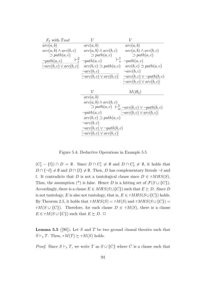
F2 with Taut
arc(a, b)arc(a, b) ∧ arc(b, c)
⊃ path(a, c)
¬path(a, c)¬arc(b, c) ∨ arc(b, c)
`2r
U
arc(a, b)arc(a, b) ∧ arc(b, c)
⊃ path(a, c)
¬path(a, c)arc(b, c) ⊃ path(a, c)¬arc(b, c)¬arc(b, c) ∨ arc(b, c)
`1s
arc(a, b)arc(a, b) ∧ arc(b, c)
⊃ path(a, c)
¬path(a, c)arc(b, c) ⊃ path(a, c)¬arc(b, c)¬arc(b, c) ∨ ¬path(b, c)¬arc(b, c) ∨ arc(b, c)
V
arc(a, b)arc(a, b) ∧ arc(b, c)
⊃ path(a, c)
¬path(a, c)arc(b, c) ⊃ path(a, c)¬arc(b, c)¬arc(b, c) ∨ ¬path(b, c)¬arc(b, c) ∨ arc(b, c)
V
`5w ¬arc(b, c) ∨ ¬path(b, c)¬arc(b, c) ∨ arc(b, c)
M(H2)
Figure 5.4: Deductive Operations in Example 5.5
(C ′2 − {l}) ∩ D = ∅. Since D ∩ C ′
1 6= ∅ and D ∩ C ′2 6= ∅, it holds that
D ∩ {¬l} 6= ∅ and D ∩ {l} 6= ∅. Then, D has complementary literals ¬l and
l. It contradicts that D is not a tautological clause since D ∈ τMHS(S).
Thus, the assumption (*) is false. Hence D is a hitting set of F(S ∪ {C}).Accordingly, there is a clause E ∈ MHS(S∪{C}) such that E º D. Since D
is not tautology, E is also not tautology, that is, E ∈ τMHS(S∪{C}) holds.
By Theorem 2.5, it holds that τMHS(S) = τM(S) and τMHS(S ∪{C}) =
τM(S ∪ {C}). Therefore, for each clause D ∈ τM(S), there is a clause
E ∈ τM(S ∪ {C}) such that E º D. 2
Lemma 5.5 ([90]). Let S and T be two ground clausal theories such that
S `s T . Then, τM(T ) º τM(S) holds.
Proof. Since S `s T , we write T as S ∪ {C} where C is a clause such that
94

D º C for some clause D ∈ S. Since D and C are ground, D ⊆ C holds.
Let C ′ and D′ be two sets such that C ′ (resp. D′) consists of the negations of
literals in C (resp. D). Note that D′ is included in F(S) since D ∈ S. Let E
be a clause in τMHS(S). E is a hitting set of F(S). Then E∩D′ 6= ∅ holds.
Since D ⊆ C, D′ ⊆ C ′ holds. Since D′ ⊆ C ′ and E ∩ D′ 6= ∅, E ∩ C ′ 6= ∅holds. Hence E is a hitting set of F(S ∪ {C}). Then there is a clause E ′ ∈MHS(S∪{C}) such that E ′ º E. Since E ∈ τMHS(S), E is not tautology.
Accordingly, E ′ is also not tautology, that is, E ′ ∈ τMHS(S ∪ {C}) holds.
By Theorem 2.5, it holds that τMHS(S) = τM(S) and τMHS(S ∪{C}) =
τM(S ∪ {C}). Therefore, for each clause E ∈ τMHS(S), there is a clause
E ′ ∈ τMHS(S ∪ {C}) such that E ′ º E. 2
Lemma 5.6 ([90]). Let S and T be two ground clausal theories such that
S `w T . Then, τM(T ) º τM(S) holds.
Proof. Since S `w T , we write T as S −{C} where C is a clause in S. Let E
be a clause in τMHS(S). E is a minimal hitting set of F(S). Since T ⊂ S,
F(T ) ⊂ F(S) holds. Then E is a hitting set of F(T ) since F(T ) ⊂ F(S).
Hence there is a clause E ′ ∈ MHS(T ) such that E ′ º E. Since E is not
tautology, E ′ is also not tautology, that is, E ′ ∈ τMHS(T ) holds. By
Theorem 2.5, it holds that τMHS(S) = τM(S) and τMHS(T ) = τM(S)
holds. Therefore, for each clause E ∈ τM(S), there is a clause E ′ ∈ τM(T )
such that E ′ º E. 2
Using Lemma 5.3, 5.4, 5.5 and 5.6, Theorem 5.4 is proved as follows:
(Proof of Theorem 5.4.) By Lemma 5.3, there are two ground clausal theories
U and V such that
S `∗r U `∗
s V `∗w T.
By Lemma 5.4, τM(U) º τM(S) holds. By Lemma 5.5, τM(V ) º τM(U)
holds. By Lemma 5.6, τM(T ) º τM(V ) holds. Hence, the following formula
holds:
τM(T ) º τM(V ) º τM(U) º τM(S). 2
Theorem 5.4 enables us to construct an alternative generalization proce-
dure using minimal complements.
95

5.3.3 Deriving Hypotheses with Induction Fields
To describe the hypotheses that can be found by this, we first introduce the
following language bias, called an induction field:
Definition 5.2 (Induction field). An induction field, denoted by IH, is de-
fined as 〈L〉 where L is a finite set of literals to be appeared in ground
hypotheses. A ground hypothesis Hg belongs to IH = 〈L〉 if every literal in
Hg is included in L.
We next define the target hypotheses using the notion of an induction
field IH, together with a bridge theory F as follows:
Definition 5.3 (Hypothesis wrt IH and F ). Let H be a hypothesis. H is
a hypothesis wrt IH and F if there is a ground hypothesis Hg such that Hg
consists of instances from H, F |= ¬Hg and Hg belongs to IH.
Now, the generalization procedure based on inverse subsumption with
minimal complements is as follows:
Definition 5.4. Let B, E and IH = 〈L〉 be a background theory, observa-
tions and an induction field, respectively. Let F be a bridge theory wrt B
and E. A clausal theory H is derived by inverse subsumption with minimal
complements from F wrt IH if H is constructed as follows.
Step 1. Taut(IH) := {¬A ∨ A | A ∈ L and ¬A ∈ L};Step 2. Compute τM(F ∪ Taut(IH));Step 3. Construct a clausal theory H satisfying the condition:
H º τM(F ∪ Taut(IH)). (3)
Inverse subsumption with minimal complements ensures the complete-
ness for finding hypotheses wrt IH and F , by way of (3).
Main Theorem ([90]). Let B, E and IH be a background theory, obser-
vations and an induction field, respectively. Let F be a bridge theory wrt
B and E. For every hypothesis H wrt IH and F , H is derived by inverse
subsumption with minimal complements from F wrt IH.
96

Proof. It is sufficient to prove the following lemma. 2
Lemma 5.7 ([90]). Let B, E and IH be a background theory, observations
and an induction field, respectively. Let F be a bridge theory wrt B and E.
For every hypothesis H wrt IH and F , H satisfies the following condition:
H º τM(F ∪ Taut(IH)).
Proof. Since H is a hypothesis wrt IH and F , there is a ground hypothesis
Hg such that H º Hg, F |= ¬Hg and Hg belongs to IH. Since ¬Hg ≡ M(Hg),
F |= M(Hg) holds. Accordingly, F ∪ Taut(IH) |= M(Hg) holds. Since
Hg belongs to IH, every literal in Hg is included in IH. Then, for every
tautological clause D ∈ M(Hg), there is a clause C ∈ Taut(IH) such that
C º D. By Theorem 5.4, τM2(Hg) º τM(F ∪ Taut(IH)) holds. Since
µHg = M2(Hg) by Theorem 3, τµHg º τM(F ∪ Taut(IH)) holds. Since
Hg ⊇ τµHg, Hg º τµHg holds. Hence, H º τM(F ∪ Taut(IH)) holds. 2
Example 5.5. We show how a target hypothesis is derived by inverse sub-
sumption with minimal complements using Example 3.3 on pathway comple-
tion:
B = {arc(a, b), arc(X,Y ) ∧ path(Y, Z) ⊃ path(X,Z)}. E = {path(a, c)}.
IH = 〈{arc(b, c), ¬arc(b, c), path(b, c), ¬path(b, c)}〉.
H = {arc(b, c), arc(X,Y ) ⊃ path(X,Y )}.
One arc from b to c and one rule on pathways are missing in B. The task, as
we explained in Chapter 3, is to find the hypothesis H that completes these
missing fact and rule. To complete H, both abduction and induction must in-
volve, but most current ILP systems cannot compute it. Let F be the clausal
theory {arc(a, b), arc(a, b)∧path(b, c) ⊃ path(a, c), ¬path(a, c)}. Since F is
the set of ground instances from B ∧¬E, F is a bridge theory wrt B and E.
Since there is a ground hypothesis Hg = {arc(b, c), arc(b, c) ⊃ path(b, c)}such that Hg consists of instances from H, F |= ¬Hg and Hg belongs to
IH, H is a hypothesis wrt IH and F . Then, H could be derived by in-
verse subsumption with minimal complements. We first compute Taut(IH).
97

Then, Taut(IH) is the set {¬arc(b, c) ∨ arc(b, c), ¬path(b, c) ∨ path(b, c)}.After adding Taut(IH) to F , we compute τM(F ∪Taut(IH)) represented as
follows.
{ ¬arc(a, b) ∨ path(b, c) ∨ arc(b, c) ∨ path(a, c),¬arc(a, b) ∨ ¬arc(b, c) ∨ path(b, c) ∨ path(a, c) }.
We then notice that H subsumes τM(F ∪ Taut(IH)) (See the dotted
surrounding parts). Therefore, H can be derived by inverse subsumption with
minimal complements. In contrast, Since R(F ) is {¬arc(a, b) ∨ path(b, c) ∨path(a, c)}, H does not subsume the residue R(F ). Hence, H cannot be
obtained from the residue complement, whereas the minimal complement
can do with inverse subsumption.
5.4 Discussion
In this section, we compare inverse subsumption with minimal complements
with the previous approach based on inverse entailment. We recall Example
5.5. In this example, we assumed the following bridge theory:
F = {arc(a, b), arc(a, b) ∧ path(b, c) ⊃ path(a, c), ¬path(a, c)}.
The residue and minimal complement τM(F ) is as follows:
τM(F ) = ¬arc(a, b) ∨ path(b, c) ∨ path(a, c).
We may notice that τM(F ) is the resolvent of two clauses C1 and C2 in
τM(F ∪ Taut(IH)):
C1 = ¬arc(a, b) ∨ path(b, c) ∨ path(a, c) ∨ arc(b, c).
C2 = ¬arc(a, b) ∨ path(b, c) ∨ path(a, c) ∨ ¬arc(b, c).
This fact means that adding a tautological clause to the bridge theory F
plays a role on an operation of inverse resolution. To deeply view the cor-
respondence between adding tautologies and inverting resolution, we recall
98
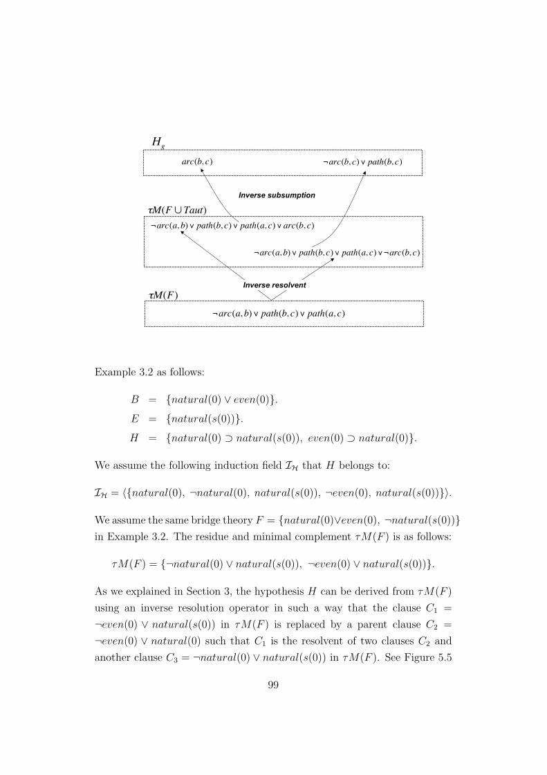
!
¬arc(a, b)" path(b, c)" path(a, c)"arc(b, c)
!
¬arc(a, b)" path(b, c)" path(a, c)"¬arc(b, c)
!
¬arc(a, b)" path(b, c)" path(a, c)
!
"M(F#Taut)!
arc(b, c)
!
¬arc(b, c)" path(b, c)
Inverse resolvent
!
Hg
!
"M(F)
Inverse subsumption
Example 3.2 as follows:
B = {natural(0) ∨ even(0)}.
E = {natural(s(0))}.
H = {natural(0) ⊃ natural(s(0)), even(0) ⊃ natural(0)}.
We assume the following induction field IH that H belongs to:
IH = 〈{natural(0), ¬natural(0), natural(s(0)), ¬even(0), natural(s(0))}〉.
We assume the same bridge theory F = {natural(0)∨even(0), ¬natural(s(0))}in Example 3.2. The residue and minimal complement τM(F ) is as follows:
τM(F ) = {¬natural(0) ∨ natural(s(0)), ¬even(0) ∨ natural(s(0))}.
As we explained in Section 3, the hypothesis H can be derived from τM(F )
using an inverse resolution operator in such a way that the clause C1 =
¬even(0) ∨ natural(s(0)) in τM(F ) is replaced by a parent clause C2 =
¬even(0) ∨ natural(0) such that C1 is the resolvent of two clauses C2 and
another clause C3 = ¬natural(0) ∨ natural(s(0)) in τM(F ). See Figure 5.5
99

!
H
!
M(F)!
C2
=¬even(0)"natural(0)
!
C3
=¬natural(0)"natural(s(0))
!
C1
=¬even(0)"natural(s(0))
Inverse resolution
Figure 5.5: Example of Inverse Resolution
which sketches the logical relation between three clauses C1, C2 and C3. In
the case of inverse subsumption with minimal complements, we first compute
τM(F ∪ Taut(IH)) as follows:
τM(F ∪ Taut(IH)) = {¬natural(0) ∨ natural(s(0)),
¬even(0) ∨ natural(0) ∨ natural(s(0))}.
We may notice that the clause ¬natural(0) ∨ natural(s(0)) in τM(F ∪Taut(IH)) corresponds to C3 in H, and another clause C4 = ¬even(0) ∨natural(0) ∨ natural(s(0)) is subsumed by C2 in H. Hence, H º µM(F ∪Taut(IH)) holds. In other words, H can be obtained from µM(F∪Taut(IH))
only by using inverse subsumption, strictly speaking, by dropping the literal
natural(s(0)) from C4. We also note that the clause C1 in τM(F ) is the re-
solvent of C3 and C4 in τM(F ∪ Taut(IH)). Hence, τM(F ∪ Taut(IH)) can
be obtained by applying an inverse resolution operator to τM(F ). This fact
implies that adding tautologies to F in fact plays a role inverting resolution.
Figure 5.6 describes the logical relation between H, τM(F ∪ Taut(IH)) and
τM(F ).
There is a well-known operator, called V − operator [47], which performs
inverting resolution. This operator is given for Horn clauses as follows:
100

!
H
!
M(F)
!
C2
=¬even(0)"natural(0)
!
C3
=¬natural(0)"natural(s(0))
!
C1
=¬even(0)"natural(s(0))
Inverse resolution
!
C4
=¬even(0)"natural(0)"natural(s(0))
Inverse subsumption
!
M(F"Taut(IH))
Figure 5.6: Inverting Resolution by Adding Tautologies
Input: Two Horn clauses C1 = L1 ∨ C ′1 and R, where C ′
1 º R.Output: A Horn clause C2, such that
R is an instance of a resolvent of C1 and C2.
Step 1. Choose a substitution θ1 such that C ′1θ1 ⊆ R.
Step 2. Choose an L2 and C ′2 such that L1θ1 = ¬L2θ2
and C ′2θ2 = R − C ′
1θ1, for some θ2.
Step 3. Let C2 = L2 ∨ C ′2.
The following figure describes the logical relation between two input
clauses C1 and R and the output clause C2.
Example 5.6. Let C1 = P (X) ∨ ¬Q(X) and R = P (f(Y )) ∨ ¬Q(Y ). We
here assume that L1 = P (X). Then, C ′1 = ¬Q(X) holds.
1. There is only one substitution θ1 such that C ′1θ1 ⊆ R, namely θ1 =
{X/Y }.
2. L2 and C ′2 should be such that, for some θ2, L1θ1 = P (Y ) = ¬L2θ2 and
R − C ′1θ1 = P (f(Y )) = C ′
2θ2. We here choose θ2 = {Z/Y }. Then, it
holds that L2 = ¬P (Z) and C ′2 = P (f(Z)).
101

!
C1
= L1"C
1'
!
C2
= L2"C
2'
!
R = C1'"1#C
2'"2
!
"1
!
"2
Figure 5.7: Setting for V-operator
3. Let C2 = L2 ∨ C ′2 = ¬P (Z) ∨ P (f(Z)).
There are several ways to select L1 and θ2. The V-operator is then non-
deterministic algorithm.
The hypothesis H in Figure 5.5 and 5.6 can be obtained by applying
a V-operator to M(F ). On the other hand, M(F ∪ Taut(IH)) itself can-
not be obtained using V-operator, though M(F ∪ Taut(IH)) should be also
obtained by inverse resolution. In this sense, V-operator is sound but incom-
plete in performing inverse resolution. Previously, it has not been studied
how inverse resolution can be completely performed due to its huge computa-
tional complexity. On the other hand, using our result to logically reduce it
into inverse subsumption, inverse resolution is embedded by add tautological
clauses associated with a given induction field to the bridge theory.
Example 5.7. Let B, E and H be a background theory, observations and
a hypothesis as follows:
B = {plus(0, 0, 0)}.
E = {plus(s(0), s(0), s2(0))}.
H = {plus(X,Y, Z) ⊃ plus(s(X), Y, s(Z)),
plus(X,Y, Z) ⊃ plus(X, s(Y ), s(Z))}.
Note that the predicate plus(X,Y, Z) means X + Y = Z. For instance, E
says 1 + 1 = 2. H corresponds to two missing rules that define the predicate
102

plus. Let F be the following bridge theory wrt B and E:
F = {plus(0, 0, 0), ¬plus(s(0), s(0), s2(0))}.
Note that F is equal to B ∪ ¬E. τM(F ) is the clause ¬plus(0, 0, 0) ∨plus(s(0), s(0), s2(0)). For deriving H from τM(F ), we need to perform
inverting resolution in some way. However, V-operator cannot be applied to
F , since F contain only one clause. Besides, any systematic operator that
enables to derive the target H has not been proposed so far. In contrast, our
approach based on inverse subsumption can give an insight to perform suf-
ficient inverse resolution by introducing an induction field IH. For instance,
let IH be as follow:
IH = 〈{ plus(0, 0, 0), ¬plus(0, 0, 0),
plus(s(0), s(0), s2(0)), ¬plus(s(0), s(0), s2(0)),
plus(s(0), 0, s(0)), ¬plus(s(0), 0, s(0))}〉.
One atom plus(s(0), 0, s(0)) is newly introduced in IH, which does not appear
in B and E. Then, τM(F ∪ Taut(IH)) is as follows:
{¬plus(0, 0, 0) ∨ plus(s(0), s(0), s2(0)) ∨ ¬plus(s(0), 0, s(0)),
¬plus(0, 0, 0) ∨ plus(s(0), s(0), s2(0)) ∨ plus(s(0), 0, s(0))}.
We notice that τM(F ) is the resolvent of two clauses in τM(F ∪Taut(IH)).
Since the target hypothesis H subsumes τM(F ∪ τTaut(IH)), it can be
obtained by dropping operators and anti-instantiation operators.
As we have described here, there has not been any proposal to inverse
resolution operators that ensure completeness for finding hypotheses so far.
For this reason, it was not straightforward to formally describe the search
space that hypothesis finding based on inverse entailment actually imposes.
Through this chapter, we have clarified that hypothesis finding based on
inverse entailment can be reduced into inverse subsumption from the minimal
complement of a bridge theory F and the tautological clauses Taut(IH).
Suppose that every target hypothesis H wrt F and IH is irredundant. In
103

other words, H−{C} is no longer a hypothesis wrt F and IH for every clause
C ∈ H. In this case, we do not need to apply any anti-weankening operators
adding arbitrary clauses to M(F ∪ Taut(IH)). Every ground hypothesis can
be obtained only by applying some dropping operators to M(F ∪Taut(IH)).
Hence, under this specific condition that the target hypotheses are ground
and irredundant, the number of possible hypotheses should be at least upper
bounded by 2n − 1 where n is the number of clauses in M(F ∪ Taut(IH)).
In this way, if we consider some typical assumption to the target hypothe-
ses, it would be possible to analyze two search spaces of inverse subsump-
tion and inverse entailment by comparing the number of possible hypotheses
obtained by each approach. For this comparison, we first give the formal
definition of inverse resolution operator as follows:
Definition 5.5 (Inverse resolution operator). Let IH = 〈L〉 be an induction
field and S a ground clausal theory belonging to IH. A ground clausal theory
T is obtained by inverse entailment from S wrt IH if T is of the form:
T = (S − {C}) ∪ {(D1 ∪ {l}), (D2 ∪ {¬l})},
where D1 and D2 are two clauses such that D1 ∪ D2 = C, and l and ¬l are
complementary literals that are not contained in C but in L.
Example 5.8. Let S be the clausal theory {{a}} and IH be 〈{a, b, ¬b, c, ¬c}〉.There are six possible clausal theories obtained by at one time applying an
inverse resolution operator to S as follows:
T1 = {{a, b}, {¬b}}. T2 = {{b}, {a, ¬b}}. T3 = {{a, b}, {a, ¬b}}.
T4 = {{a, c}, {¬c}}. T5 = {{c}, {a, ¬c}}. T3 = {{a, c}, {a, ¬c}}.
Assume that S contains only one clause C that has n literals. Each literal
in C can be included in either D1, D2 or both D1 and D2. That is why
there are 3n ways to apply an inverse resolution operator at one time for
each complementary literal in IH. Hence, the total number of possible ways
to apply an inverse resolution operator at one time should be 3n × m where
m is the number of pairs of complemental literals in a given induction field.
104
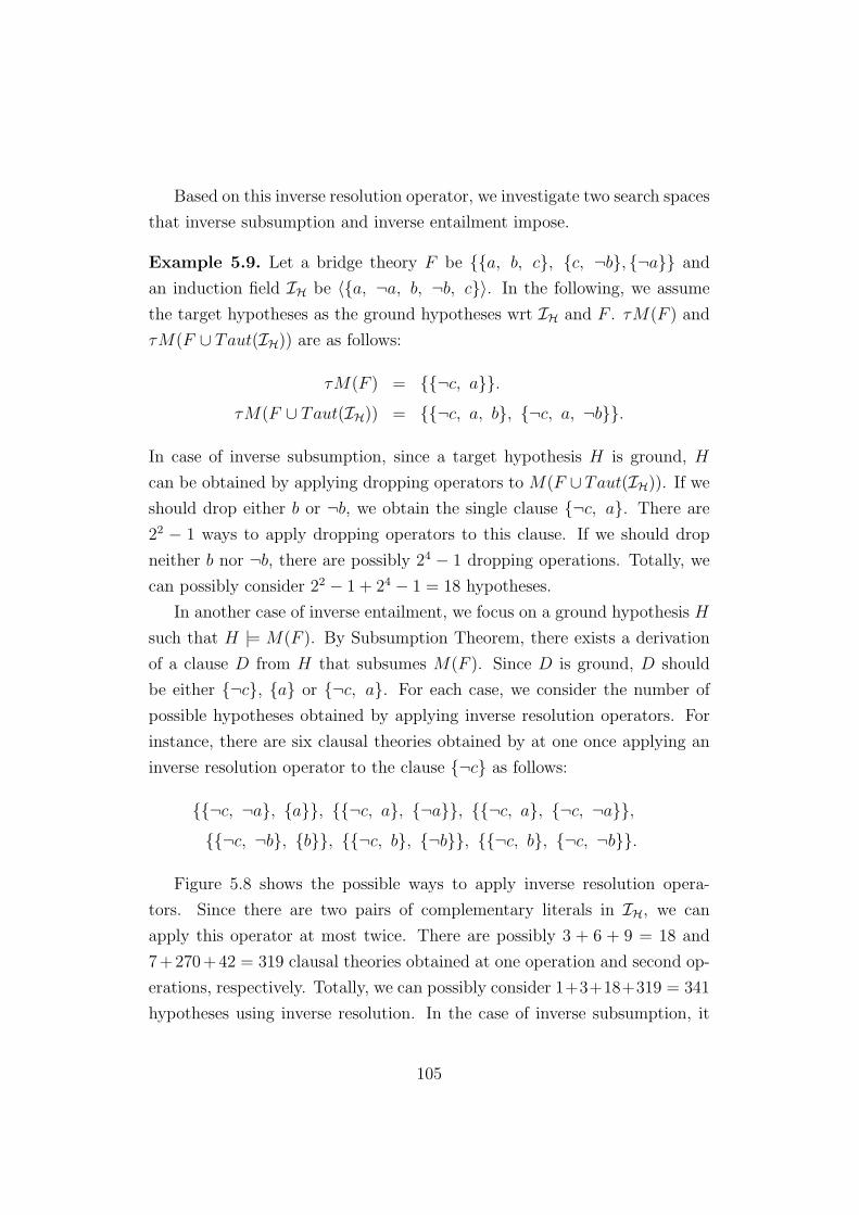
Based on this inverse resolution operator, we investigate two search spaces
that inverse subsumption and inverse entailment impose.
Example 5.9. Let a bridge theory F be {{a, b, c}, {c, ¬b}, {¬a}} and
an induction field IH be 〈{a, ¬a, b, ¬b, c}〉. In the following, we assume
the target hypotheses as the ground hypotheses wrt IH and F . τM(F ) and
τM(F ∪ Taut(IH)) are as follows:
τM(F ) = {{¬c, a}}.
τM(F ∪ Taut(IH)) = {{¬c, a, b}, {¬c, a, ¬b}}.
In case of inverse subsumption, since a target hypothesis H is ground, H
can be obtained by applying dropping operators to M(F ∪ Taut(IH)). If we
should drop either b or ¬b, we obtain the single clause {¬c, a}. There are
22 − 1 ways to apply dropping operators to this clause. If we should drop
neither b nor ¬b, there are possibly 24 − 1 dropping operations. Totally, we
can possibly consider 22 − 1 + 24 − 1 = 18 hypotheses.
In another case of inverse entailment, we focus on a ground hypothesis H
such that H |= M(F ). By Subsumption Theorem, there exists a derivation
of a clause D from H that subsumes M(F ). Since D is ground, D should
be either {¬c}, {a} or {¬c, a}. For each case, we consider the number of
possible hypotheses obtained by applying inverse resolution operators. For
instance, there are six clausal theories obtained by at one once applying an
inverse resolution operator to the clause {¬c} as follows:
{{¬c, ¬a}, {a}}, {{¬c, a}, {¬a}}, {{¬c, a}, {¬c, ¬a}},
{{¬c, ¬b}, {b}}, {{¬c, b}, {¬b}}, {{¬c, b}, {¬c, ¬b}}.
Figure 5.8 shows the possible ways to apply inverse resolution opera-
tors. Since there are two pairs of complementary literals in IH, we can
apply this operator at most twice. There are possibly 3 + 6 + 9 = 18 and
7+270+42 = 319 clausal theories obtained at one operation and second op-
erations, respectively. Totally, we can possibly consider 1+3+18+319 = 341
hypotheses using inverse resolution. In the case of inverse subsumption, it
105
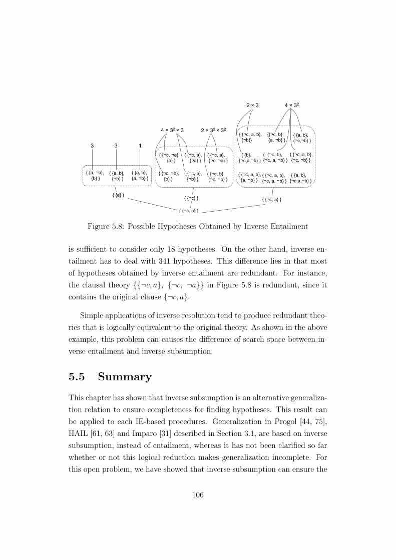
{ {¬c, a} }
{ {a} } { {¬c} } { {¬c, a} }
{ {a, ¬b}, {b} }
{ {a, b}, {¬b} }
{ {a, b}, {a, ¬b} }
{ {¬c, ¬b}, {b} }
{ {¬c, b}, {¬b} }
{ {¬c, b}, {¬c, ¬b} }
{ {¬c, ¬a}, {a} }
{ {¬c, a}, {¬a} }
{ {¬c, a}, {¬c, ¬a} }
{ {¬c, a, b}, {a, ¬b} }
{ {¬c, a, b}, {¬c, a, ¬b} }
3 3
4 × 32 × 3 2 × 32 × 32
4 × 322 × 3
1
{ {a, b}, {¬c,a,¬b} }
{{¬c, b}, {a, ¬b} }
{ {¬c, b}, {¬c, a, ¬b} }
{ {b}, {¬c,a,¬b} }
{ {¬c, a, b}, {¬b}}
{ {¬c, a, b}, {¬c, ¬b} }
{ {a, b}, {¬c,¬b} }
Figure 5.8: Possible Hypotheses Obtained by Inverse Entailment
is sufficient to consider only 18 hypotheses. On the other hand, inverse en-
tailment has to deal with 341 hypotheses. This difference lies in that most
of hypotheses obtained by inverse entailment are redundant. For instance,
the clausal theory {{¬c, a}, {¬c, ¬a}} in Figure 5.8 is redundant, since it
contains the original clause {¬c, a}.
Simple applications of inverse resolution tend to produce redundant theo-
ries that is logically equivalent to the original theory. As shown in the above
example, this problem can causes the difference of search space between in-
verse entailment and inverse subsumption.
5.5 Summary
This chapter has shown that inverse subsumption is an alternative generaliza-
tion relation to ensure completeness for finding hypotheses. This result can
be applied to each IE-based procedures. Generalization in Progol [44, 75],
HAIL [61, 63] and Imparo [31] described in Section 3.1, are based on inverse
subsumption, instead of entailment, whereas it has not been clarified so far
whether or not this logical reduction makes generalization incomplete. For
this open problem, we have showed that inverse subsumption can ensure the
106

completeness only by adding tautological clauses associated with a language
bias to a bridge theory. The generalization of Residue procedure [83] cor-
responds to inverse subsumption with residue complements, which has been
studied in Section 5.3. In Section 5.4, we have discussed about the corre-
spondence between inverting resolution and adding tautological clauses and
showed that the task of V -operator, which has been previously proposed for
inverse resolution, can be achieved by using inverse subsumption. We have
also analyzed the search space in each case of inverse entailment and in-
verse subsumption with minimal complement using a concrete example. As
a result, we have showed that the search space in inverse subsumption with
minimal complements could be indeed less than the one in inverse entailment.
CF-induction uses inverse entailment as the generalization relation. Hence,
the generalization of CF-induction can be reduced into inverse subsumption
with minimal complements. In next chapter, we investigate the general-
ization procedure of CF-induction and logically reconstruct it into a more
simplified form based so as to reduce the non-determinism in CF-induction.
107

Chapter 6
Logical Reconstruction inCF-induction
6.1 Introduction
CF-induction preserves soundness and completeness of finding hypotheses
in full clausal theory. Compared with the other IE-based methods, CF-
induction has three important benefits. Unlike Progol [44], HAIL [61] and
Imparo [31], it enables the solution of more complex problems in richer knowl-
edge representation formalisms beyond Horn logic. The motivating problem,
provided in Chapter 4, is indeed described in non-Horn clausal logic. Unlike
FC-HAIL [63], CF-induction is complete for finding full clausal hypotheses.
In Chapter 4, using this feature, we have shown that CF-induction can inte-
grate abduction and induction in biological inference of metabolic pathways.
Unlike the residue procedure [83], CF-induction can exploit language bias to
specify the search space so as to focus the procedure on some relevant part.
The derivation process in CF-induction can be described as follows: Note
@@ -B ∧ ¬E |= · · · |= CC (Generalization operations)
¬CC =| U1 =| · · · =| Un =| H
Figure 6.1: Hypothesis Finding in CF-induction
that CC is a bridge theory of CF-induction. After constructing a bridge the-
ory CC, its negation translated into CNF is generalized using a variety of
108
generalizers, as shown in Chapter 3. Any combination of generalizers can
be also soundly applied as another generalizer. Indeed, a particular hypoth-
esis H requires several different generalizers in some specific order like the
generalization operations in Figure 6.1. This fact that these generalizers can
be sequenced in many different ways makes generalization of CF-induction
highly non-deterministic.
Our objective is to reduce the non-determinism of CF-induction in order
to make the procedure easier to apply in real-world applications. In this
chapter, we concentrate on simplifying the process of obtaining hypotheses
from a bridge theory. In particular, we propose two approaches for simplifi-
cation of CF-induction. The first approach is based on the observation that
the negated hypothesis ¬H can be computed deductively from CC, i.e.,
CC |= V1 |= V2 |= · · · |= Vm−1 |= Vm |= ¬H. (6.1)
In the interests of computational efficiency, it is convenient to work in
clausal form logic. For instance, ¬H can be represented as the minimal
complement of Hsk in which any existentially quantified variables in ¬H are
substituted by ground Skolem constants. Therefore, the first approach works
in three steps: first G is deduced from CC; then it is negated; and finally
anti-instantiation is used to result in the final hypothesis H.
To derive G from CC, we introduce a new deductive operator, which
can be regarded as simplifying the existing operators of subsumption, res-
olution and weakening that we have introduced in Chapter 5. This new
operator, called the γ-operator, warrants the insertion of literals into the
clauses of CC. We show that this single deductive operator (followed by
negation and anti-instantiation) is sufficient to preserve the soundness and
completeness of CF-induction. This new approach, called CF-induction with
γ-operator, simplifies the original CF-induction in the sense that it only re-
quires one deductive operator (γ-operator) and one generalization operator
(anti-instantiation) to be used in the construction of H from CC.
The second approach is based on inverse subsumption with minimal sub-
sumption. Using the result in Chapter 5, any hypothesis can be inductively
109

derived from the minimal complement of CC ∪ Taut, i.e.,
τM(CC) ¹ R1 ¹ R2 ¹ · · · ¹ Rk−1 ¹ Rk ¹ µH. (6.2)
To use Formula 6.2, we need to logically connect production fields with
induction fields that will be extended so as to describe the syntax of target
hypotheses.
In this chapter, we also investigate another non-deterministic procedure:
construction of bridge theories. Since a bridge theory in CF-induction is de-
fined as a subset of the characteristic clauses, the number of choice points
can exponentially increase in accordance with the number of characteristic
clauses. This combinatorial explosion makes the construction of bridge the-
ories highly non-deterministic. For this problem, we propose a deterministic
way, while it preserves completeness for finding hypotheses in CF-induction.
The rest of this chapter is organized as follows. Section 6.2 describes
the first approach based on deductive operations. Section 6.3 describes the
second approach based on inverse subsumption. In Section 6.3, we also show
a deterministic way to construct bridge theories, and Section 6.4 compares
two approaches using several examples. Section 6.5 concludes.
6.2 CF-induction with Deductive Operations
Our motivation in this section is to develop a simplified generalization proce-
dure for CF-induction that uses fewer operators while preserving its sound-
ness and completeness for finding hypotheses. We present one way to simplify
the generalization process by computing generalizations deductively. Our
approach is motivated by recalling the following deductive operators, which
have been introduced in Chapter 5.
1. (resolution) T = S∪{C}, where C is a resolvent of clauses D1, D2 ∈ S.
2. (subsumption) T = S ∪ {C}, where C is subsumed by some clause
D ∈ S.
3. (weakening) T = S − {D} for some clause D ∈ S.
110

Two special cases of the subsumption operator can be further distinguished
by the following two operators.
2a (instantiation) T = S ∪ {Dσ} for some clause D ∈ S and substitution
σ.
2b (expansion) T = S ∪{C}, where C is a superset of some clause D ∈ S.
We write S `r T , S `s T , S `w T , S `α T and S `β T to denote that T is
directly derivable from S by resolution, subsumption, weakening, instantia-
tion and expansion, respectively. `∗X is the reflexive and transitive closure of
`X , where X is one of the symbols r, s, w, α, β.
We mention the following two properties concerned with reordering of
deductive operators.
Proposition 6.1 ([92]). Let U1 and U2 be clausal theories. If U1 `∗s U2, then
there exist two clausal theories V1 and V2 such that U1 `∗α V1 `∗
β V2 `∗w U2.
Proof. By Definition 5.1, there exist a substitution σi and a clause Di ∈ U1
such that Diσi ⊆ Ci, for each clause Ci ∈ U2 − U1 (1 ≤ i ≤ n). Let T be a
finite set∪n
i=1{Diσi}. Let V1 be U1 ∪ T and V2 be V1 ∪ {C1, . . . , Cn}. Then
it holds that U1 `∗α V1 and V1 `∗
β V2. Moreover, since it holds that U2 ⊆ V2,
it holds that V2 `∗w U2. 2
Proposition 6.2 ([92]). Let S, U and V be clausal theories. If S `∗w U `∗
s V ,
then there exists a clausal theory U ′ such that S `∗s U ′ `∗
w V .
Proof. Let U ′ be the clausal theory S∪ (V −U). Since U `∗s V , there exists a
clause Di ∈ U such that Di º Ci for each clause Ci ∈ V − U . Since S `∗w U ,
U ⊆ S holds. Since Di ∈ U , Di ∈ S holds. Therefore U ′ is obtained from S
using the subsumption operator, that is, S `∗s U ′. Next we show that V ⊆ U ′
holds. Since U ′ = S ∪ (V − U), V − U ⊆ U ′ holds. And also, S ⊆ U ′ holds.
Since S `∗w U , U ⊆ S holds. Accordingly, V ∩U ⊆ U ′ holds, since V ∩U ⊆ U .
Since V − U ⊆ U ′ and V ∩ U ⊆ U ′, V ⊆ U ′ holds. Hence U ′ `∗w V holds. 2
We use the above ordering results as well as Theorem 5.5 to show how
the number of generalization operators used in CF-induction can be reduced.
Section 6.2.1 shows this result in the case of ground hypotheses and Section
6.2.2 shows it in the general case.
111

6.2.1 Logical Relation Between Bridge Theoriesand Ground Hypotheses
First, we show that resolution and instantiation can be incorporated into the
selection of CC. We show this with the following two lemmas.
Lemma 6.1 ([92]). Let CC be a bridge theory wrt B, E and P , and U be a
clausal theory. If CC `∗r U , then there exist a clausal theory V and a bridge
theory CC ′ wrt B, E and P such that CC ′ `∗s V `∗
w U .
Proof. The proof is in two parts.
(a) First we prove that, for each clause Ci ∈ U (1 ≤ i ≤ n), there exists
a clause Di ∈ Carc(B ∧ E,P) such that Di º Ci.
By the definition of characteristic clauses, for each clause K ∈ ThP(B∧E)
there exists a clause M ∈ Carc(B ∧ E,P) such that M º K. Hence it is
sufficient to show that every clause Ci ∈ U is included in ThP(B ∧E). Since
CC |= U and B∧E |= CC, it holds that every clause Ci ∈ U is a consequence
of B ∧ E. Then it remains to show that every clause Ci ∈ U belongs to P ,
which is done by mathematical induction on the number n of the applications
of `r for deriving U from CC. In the following, we write CC `nr U to denote
that U is derived from CC by n applications of `r.
Base step: If n = 0 then U = CC and it trivially follows that every clause
in U belongs to P.
Induction step: If n = k+1 for some k ≥ 0, then it holds that CC `kr U ′ `r U
where U ′ is a clausal theory. By the induction hypothesis, it holds that
every clause in U ′ belongs to P . Moreover, it follows that U = U ′∪{R}for some resolvent R of two clauses in U ′. Since every clause in U ′
belongs to P and P is closed under instantiation, the resolvent R also
belongs to P . Thus every clause in U belongs to P and so part (a)
holds.
(b) Now we show how to construct the theories CC ′ and V . Start by
defining the theory T =∪n
i=1{Di} using the clauses Di ∈ Carc(B ∧ E,P)
constructed above. Now define the bridge theory CC ′ = CC ∪ T and the
112

theory V = CC ′ ∪ U . Since for each clause Ci ∈ U there exists Di ∈ T
such that Di º Ci, CC ′ `∗s V holds. Since U ⊆ V , V `∗
w U holds. Hence
CC ′ `∗s V `∗
w U holds. Each clause in CC ′ is an instance of a clause in
Carc(B ∧E,P). Since CC ⊆ CC ′ and CC is a bridge theory, there exists a
clause in CC ′ which is an instance of a clause in NewCarc(B, E,P). Then
CC ′ is a bridge theory. Therefore there exist a bridge theory CC ′ and a
clausal theory V such that CC ′ `∗s V `∗
w U . 2
Lemma 6.2 ([92]). Let CC be a bridge theory wrt B, E and P , and U be
a clausal theory. If CC `∗α U , then U is a bridge theory wrt B, E and P .
Proof. Every clause in U is an instance of a clause in Carc(B ∧E,P). Since
U ⊇ CC, there exists a clause Ci ∈ U such that Ci is an instance of a clause
from NewCarc(B, E,P). Therefore, U is a bridge theory. 2
Then, using Lemmas 6.1 and 6.2, we can show the following theorem,
which establishes the logical relation between bridge theories and ground
hypotheses.
Theorem 6.1 ([92]). Let H be a ground hypothesis wrt B, E and P . Then
there exist a bridge formula CC wrt B, E and P and a clausal theory V such
that CC `∗β V `∗
w H.
Proof. First, we consider the case that H has no tautological clauses. Then,
by Theorem 3.1, there exists a bridge theory CC such that CC |= ¬H.
Since H is ground, H ≡ ¬H holds. Thus CC |= H holds. By Theorem
5.5, there exist clausal theories V1 and V2 such that CC `∗r V1 `∗
s V2 `∗w H.
By Lemma 6.1, there exist a clausal theory V3 and a bridge formula CC ′′
such that CC ′′ `∗s V3 `∗
w V1 `∗s V2 `∗
w H. By Proposition 6.2, there ex-
ists a clausal theory V4 such that CC ′′ `∗s V3 `∗
s V4 `∗w V2 `∗
w H. Thus
CC ′′ `∗s V4 `∗
w H. By Proposition 6.1, there exist clausal theories V5 and
V6 such that CC ′′ `∗α V5 `∗
β V6 `∗w V4 `∗
w H. By Lemma 6.2, V5 is a bridge
theory, and by letting CC ′ = V5, it holds that CC ′ `∗β V6 `∗
w H.
Next, in the case that H contains tautological clauses, we let T = {D1, . . . , Dn}denote the set of the tautological clauses in H. Then, since every clause
Di ∈ T (1 ≤ i ≤ n) is a consequence of B ∧ E and Di belongs to P , for
113

each Di ∈ T there exists a clause Ci ∈ Carc(B ∧ E,P) such that Ci º Di.
Let S be the clausal theory∪n
i=1{Ci}. Then, it holds that S `∗s S1 `∗
w T
where S1 = S ∪ T . Now, since the clausal theory H − T has no tautological
clauses, there exist a bridge theory CC and a clausal theory V7 such that
CC `∗s V7 `∗
w H −T . Then, it holds that CC ∪S `∗s V7 ∪S1 `∗
w H. Since the
clausal theory CC ∪ S satisfies Definition 3.4, the theorem holds. 2
Next, we introduce a new operator, which can be regarded as concate-
nating weakening and expansion.
Definition 6.1. [γ-operator] Let S and T be clausal theories. T is directly
γ-derivable from S iff T is obtained from S under the following condition:
T = (S − {D}) ∪ {C1, . . . , Cn}
for some n ≥ 0 where Ci ⊇ D for all 1 ≤ i ≤ n.
Analogously to Definition 5.1, we write S `γ T iff T is directly γ-derivable
from S and `∗γ is a reflexive and transitive closure of `γ.
Theorem 6.2 ([92]). Let H be a ground hypothesis wrt B, E and P . Then,
there exists a bridge formula CC wrt B, E and P such that CC `∗γ H.
Proof. Since H is a ground hypothesis, by Theorem 6.1, there exist a bridge
theory CC = {C1, . . . , Cn} and a clausal theory U such that CC `∗β U `∗
w H.
Let FCibe the clausal theory {C | C ∈ H and Ci ⊆ C}, for each clause
Ci ∈ CC (1 ≤ i ≤ n). Then, by Definition 6.1, for each clause Ci ∈ CC,
{Ci} `∗γ FCi
holds. Accordingly, CC `∗γ
∪ni=1 FCi
holds. Hence, it is sufficient
to show that H =∪n
i=1 FCi. Since FCi
⊆ H for every clause Ci ∈ CC, it holds
that∪n
i=1 FCi⊆ H. Conversely, since CC `∗
β U , for every clause D ∈ U ,
there exists a clause Ci ∈ CC such that Ci ⊆ D. Also since U `∗w H, it holds
that H ⊆ U . Then, for every clause D ∈ H, there exists a clause Ci ∈ CC
such that Ci ⊆ D, that is, D ∈ FCi. This means that H ⊆
∪ni=1 FCi
. Hence,
it holds that H =∪n
i=1 FCi. Therefore, it holds that CC `∗
γ H. 2
114

6.2.2 Deriving Non-Ground Hypotheses
We generalize the result of the previous section to non-ground hypotheses.
We show that any hypothesis can be obtained from a bridge theory by ap-
plying the γ-operator followed by anti-instantiation.
Definition 6.2. Let B and E be clausal theories and P = 〈L〉 be a produc-
tion field. A clausal theory H is derived by CF-induction with γ-operator
from B, E and P iff H is constructed as follows:
Input: A background theory B, observations Eand a production field P .
Output: A hypothesis H wrt B, E and P .
Step 1. Construct a bridge theory CC wrt B, E and P.
Step 2. Construct a clausal theory G such that CC `∗γ G.
Step 3. Compute the complement G of G.
Step 4. H is obtained by applying anti-instantiation to G,
such that (1) B ∧ H is consistent,
(2) H contains no Skolem constants, and
(3) for every literal L in H, ¬L belongs to P.
Several remarks are necessary for Definition 6.2.
Step 2. Even if G satisfies CC `∗γ G for some bridge theory CC, any output
H obtained from G cannot satisfy the conditions of Definition 3.1 unless
G∧B is consistent and G belongs to P. In this respect, the constraints
of H at Step 4 are introduced to guarantee the soundness of H.
Step 3. The complement of G can theoretically include redundant clauses
such as tautological clauses and clauses properly subsumed by other
clauses. Accordingly it might be sufficient to use minimal and residue
complements, instead of complements.
Step 4. Anti-instantiation allows us to replace subterms in G with variables.
For example, for the clause p(a)∨q(a), it is possible to construct p(X)∨
115

q(Y ) obtained by replacing the constant a in p(a) and q(a) with two
variables X and Y , respectively. In this way there are many possibilities
to apply anti-instantiation for clauses.
We now give soundness and completeness results for CF-induction with
γ-operator.
Theorem 6.3 ([92]). [Soundness] Let B, E and H be clausal theories, and
P be a production field. If H is derived by CF-induction with γ-operator
from B, E and P , then H is a hypothesis wrt B, E and P .
Proof. Suppose a clausal theory H is derived by CF-induction with γ-
operator from B, E and P . Then, by Definition 6.2, there exist a bridge
theory CC and a clausal theory G such that H is derived by applying
anti-instantiation to G and CC `∗γ G. By Definition 3.4, it holds that
B ∧ E |= CC. By Definition 6.1, it holds that CC |= G. Accordingly, it
holds that B ∧ E |= G. Since H is derived by applying anti-instantiation to
G, H |= G holds. Since G |= ¬G, H |= ¬G follows. Equivalently, G |= ¬H.
Therefore, it holds that B ∧ E |= ¬H. Then, it holds that B ∧ H |= ¬E.
Since, from Step 4 of Definition 6.2, H contains no Skolem constants from
E, it holds that B ∧ H |= E. Hence, it holds that H is a hypothesis wrt B,
E and P , since, from Step 4 of Definition 6.2, B ∧ H is consistent and for
every literal L appearing in H, ¬L ∈ L. 2
Theorem 6.4 ([92]). [Completeness] Let B, E and H be clausal theories,
and P be a production field. If H is a hypothesis wrt B, E and P , then there
exists a theory H∗ ≡ H that is derived by CF-induction with γ-operator from
B, E and P .
Proof. Suppose H is a hypothesis wrt B, E and P . By Theorem 3.1, there
is a bridge theory CC wrt B, E and P such that CC ∪ H is unsatisfiable.
Using Herbrand’s theorem, there are two finite sets CC ′ and H ′ such that
CC ′ (resp. H ′) is a finite set of ground instances of CC (resp. H) and
CC ′ ∪ H ′ is unsatisfiable. In this case, H ′ can be chosen in such a way that
for every clause C in H, there is an instance C ′ of C such that C ′ ∈ H ′, and
116

also, CC ′ can be chosen in such a way that CC ′ contains at least one instance
of a clause in NewCarc(B, E,P). Then, H can be obtained by applying an
anti-instantiation generalizer to H ′. We prove that H ′ is a ground hypothesis
wrt B, E, and P . That is, we will show that (1) B∧H ′ |= E, (2) B∧H ′ 6|= 2
and (3) ¬L ∈ L for every literal L appearing in H ′.
Proof of (1): CC is a bridge theory wrt B, E and P. Since every clause
in CC ′ is an instance of a clause in CC, CC ′ satisfies the first condition of
Definition 3.4. Also, CC ′ contains at least one clause C ′ such that C ′ is an
instance of a clause from NewCarc(B, E,P). Then CC ′ satisfies the second
condition of Definition 3.4. Hence, CC ′ is also bridge theory wrt B, E and
P . Thus B ∧ E |= CC ′ holds. By CC ′ |= ¬H ′, B ∧ E |= ¬H ′ holds. Then
B ∧ H ′ |= ¬E holds. By ¬E ≡ E, B ∧ H |= E holds.
Proof of (2): If it holds that B∧H ′ |= 2, then it must hold that B∧H |= 2,
by B ∧ H |= B ∧ H ′. It contradicts the fact H is a hypothesis.
Proof of (3): Since H is a hypothesis wrt B, E and P , for every literal L
appearing in H, ¬L ∈ L holds. Then it holds that ¬L ∈ L for every literal
L appearing in H ′, since P = 〈L〉 is closed under instantiation.
Now, since H ′ is a ground hypothesis wrt B, E and P , there exists a
bridge theory CC ′′ wrt B, E and P such that CC ′′ `∗γ H ′ by Theorem 6.2.
Since E ≡ E, it holds that for every clause C in Carc(B ∧ E,P), C is
contained in Carc(B ∧ E,P). Then, it also holds that for every clause C in
CC ′′, C is contained in Carc(B∧E,P). Hence, CC ′′ is also bridge theory wrt
B, E and P . Then, from Step 1 of Definition 6.2, CC ′′ can be constructed
in a CF-induction with γ-operator from B, E and P. Moreover, H ′ can be
also constructed from CC ′′ at Step 2. Since H ′ is ground, it holds that H ′
is logically equivalent to H ′ computed from H ′ at Step 3. Recall that H
is obtained by applying anti-instantiation to H ′. Therefore a formula H∗ is
obtained at Step 4 with the application of anti-instantiation to H ′ such that
H∗ ≡ H. 2
Example 6.1. Recall Example 3.2. Let CC be the following bridge theory,
which appears in Example 3.2.
CC = (natural(0) ∨ even(0)) ∧ ¬natural(s(0)).
117
Assume that a γ-operator is applied to CC so that ¬natural(s(0)) is re-
placed with the two clauses ¬natural(s(0))∨¬even(0) and ¬natural(s(0))∨natural(0), then the following clausal theory G1 is constructed:
G1 = (natural(0) ∨ even(0))
∧ (¬natural(s(0)) ∨ ¬even(0))
∧ (¬natural(s(0)) ∨ natural(0)).
Then, we can obtain the complement G1 of G1, which is logically equivalent to
F ′1 in Example 3.2. Next assume that another γ-operator is applied to CC so
that ¬natural(s(0)) is replaced with the two clauses ¬natural(s(0))∨even(0)
and ¬natural(s(0)) ∨ ¬natural(0), then the following clausal theory G2 is
constructed:
G2 = (natural(0) ∨ even(0))
∧ (¬natural(s(0)) ∨ even(0))
∧ (¬natural(s(0)) ∨ ¬natural(0))
Then, the complement G2 of G2 is logically equivalent to F ′2 in Example 3.2.
Accordingly, we can obtain a clausal theory, which is logically equivalent to
F ′3 in Example 3.2 by applying an anti-instantiation generalizer to G2. In
this way, the inverse resolution generalizer can be realized with applications
of the γ-operator.
6.2.3 Related Work
The γ-operator can be regarded as a particular downward refinement operator
[3, 34, 41, 52] for the `∗γ order, which is closely related to the subsumption
order. Let S and T be clausal theories such that S `∗γ T . Then S º T
holds. Compared with the subsumption order, one important feature of γ-
operator lies in restraint of the operation of instantiation, which leads to a
large number of choice points. There are certain desirable properties that a
“good” downward refinement operator should satisfy and we intend to study
which of these the γ-operator satisfies.
118

We can reduce generalization under the entailment relation in the pre-
vious version to generalization under the γ-operator. It is based on the
notion that any series of processes of inductive operations on the inverse re-
lation of entailment between the negation of a bridge theory and a hypothesis
connects a certain series of processes of deductive operations on entailment
between a bridge theory and the negation of hypothesis. Accordingly, there
are two sides where we can grasp generalization processes. Yamamoto and
Fronhoefer [84] and Yamamoto [83] first have studied the connection between
two clausal theories related by entailment and negation. It will be interesting
to consider about the relation between two clausal theories ordered by the
γ-operator instead of entailment and these negations.
6.3 CF-induction with Inverse Subsumption
This section investigates how CF-induction can compute target hypotheses
based on inverse subsumption with minimal complements. Inverse subsump-
tion ensures the completeness of finding hypotheses with respect to a given
induction field. An induction field is used to describe possible literals ap-
peared in ground hypotheses. In contrast, a production field used in CF-
induction describes possible literals appeared in the negations of hypotheses.
We thus need to connect induction fields with production fields.
6.3.1 Logical Relation between Production Fieldsand Induction Fields
We first extend the definition of induction fields, which has been defined in
Section 5.3.3, into a richer representation formalization so as to describe not
only literals to be possibly included, but also the syntactical structure of
ground hypotheses like the number and length of clauses.
Definition 6.3. [Extended induction field]An extended induction field IH
is a triple 〈L, num, len〉 where L is the set of literals to be appeared in
ground hypotheses, and num and len are the maximum number and length
of clauses in ground hypotheses, respectively. A ground hypothesis Hg belongs
119

to IH = 〈L, num, len〉 iff every literal in Hg is included in L, the number of
clauses in Hg is less than or equal to num and for every clause C ∈ Hg, the
length of C is less than or equal to len. In the following, we simply refer
to an induction field, instead of an extended induction field, if no confusion
arises.
Note that the induction field is regarded as an extension of the previous
language bias obtained by adding the information on the number and length.
Based on this language bias, we define target hypotheses as follows.
Definition 6.4. [Hypothesis wrt B, E and IH] Let B, E and IH be a back-
ground theory, observations and an induction field, respectively. A clausal
theory H is a hypothesis wrt B, E and IH iff there is a ground hypothesis
Hg wrt B and E such that Hg consists of ground instances from H and Hg
belongs to IH.
We then reconstruct the conditions of bridge theories by reflecting the
induction field as follows:
Definition 6.5. [Bridge theory wrt B, E and IH] Let B, E and IH =
〈L, num, len〉 be a background theory, observations and an induction field.
A clausal theory CC is a bridge theory wrt B, E and IH iff CC is a bridge
theory wrt B, E and the production field PI = 〈L, max length ≤ num〉such that CC contains at most lennum clauses.
Note that L is the set of negations of literals in L. If no confusion arises,
a “bridge theory wrt B, E and IH” will simply be called a “bridge theory”.
Theorem 6.5 ([89]). Let B, E and IH be a background theory, observations
and an induction field. Then, for any hypothesis H wrt B, E and IH, there
exists a bridge theory CC wrt B, E and IH such that H |= ¬CC.
Proof. We write IH = 〈L, num, len〉. Since H is a hypothesis wrt B, E
and IH, there is a ground hypothesis Hg wrt B and E such that H º Hg
and Hg belongs to IH. Assume the production field P1 = 〈L〉. Then, Hg
belongs to P1. Hence, there is a bridge theory CC wrt B, E and P1 such
120

that CC |= ¬Hg. Since Hg is ground, ¬Hg ≡ Hg holds. Since the maximum
number and length of clauses in Hg are num and len, respectively, it holds
that every clause in Hg is less that or equal to num and Hg contains at most
lennum clauses. Since B ∧¬Esk |= CC and CC |= Hg, B ∧¬Esk |= Hg holds.
Hence, for each clause C in Hg, there is a clause D in Carc(B∧Esk,P1) such
that D º C. Since the length of the clause D is less than or equal to num,
D belongs to the production field PI . 2
6.3.2 Deriving Hypotheses with Induction Fields
In the original CF-induction, the bridge theory was selected by hand. Assume
that we have n characteristic clauses of B ∧ ¬E. The number of possible
bridge theories is briefly 2n. It is difficult to sufficiently choose one from a
large number of possible theories. Here, we show an incremental way for
constructing bridge theories that is deterministic and also preserving the
soundness and completeness in CF-induction. First, we recall Theorem 5.4.
Let S be a ground clausal theory and C a clause in S. By Theorem 5.4,
τM(S − {C}) º τM(S) holds.
Let B, E and IH be a background theory, observations and an induction
field. Let the list L be 〈C1n, C2
n, . . . , Cmn , C1
c , C2c , . . . , C
rc 〉 where Ci
n (1 ≤ i ≤m) and Cj
c (1 ≤ j ≤ r) is an instance of a clause in Carc(B ∧ ¬E,PI)
and NewCarc(B,¬E,PI), respectively. Note that since the set L of PI =
〈L, max length ≤ num〉 contains a finite number of ground literals, the
number of (new) characteristic clauses should be also finite.
Assume the bridge theory CCk consisting of the clauses from C1n to Ck
x in
the list L where if k ≤ m, the symbol x is equal to the symbol n, otherwise,
x is equal to the symbol c. Then, CCk ⊃ CCk−1 holds. By Theorem 5.4,
τM(CCk−1) º τM(CCk) holds.
This fact implies that the residue and minimal complement of the previ-
ous CCk−1 can be obtained by residue and minimal complement of the cur-
rent CCk using inverse subsumption. Hence, every hypothesis obtained from
CCk−1 can be also obtained from CCk. In other words, given a sufficient
121

number k, any hypothesis can be obtained by inverse subsumption from the
residue and minimal complement of τM(CCk).
Based on this notation, we can consider an alternative hypothesis finding
procedure of CF-induction that computes hypotheses wrt B, E and IH using
inverse subsumption with minimal complements as follows:
Definition 6.6. Let B and E be clausal theories and IH be an extended
induction field. A clausal theory H is derived by CF-induction with inverse
subsumption from B, E and IH iff H is constructed as follows:
Input: A background theory B, observations Eand an extended induction field IH = 〈L, num, len〉.
Output: A hypothesis H wrt B, E and IH.
Step 1. Translate IH into PI = 〈L, max length ≤ num〉.
Step 2. Compute Carc(B ∧ Esk,PI) = 〈C1, C2, . . . , Cn〉.Step 3. i := 0 and CC0 := ∅.Step 4. CCi+1 := CCi ∪ {Ci+1}.Step 5. Compute τM(CCi+1).
Step 6. If necessary, return a clausal theory H such that
(1) H belongs to IH,
(2) H º τM(CCi+1), and
(3) B ∧ H is consistent.
Else, i := i + 1 and go to Step 4.
6.4 Comparison
In Section 6.2 and 6.3, we have studied two approaches for deriving a hy-
pothesis H from a bridge theory CC in CF-induction. In the first approach
based on deductive operations, we first search the complement H such that
CC `∗γ H, and then compute the original H by translating ¬H into a CNF
formula. It would be sufficient for this dualization task to use minimal com-
plements, instead of complements, since minimal complements enables to
obtain the original hypothesis (that is, M(M(H)) = µH) by Theorem 5.3.
122
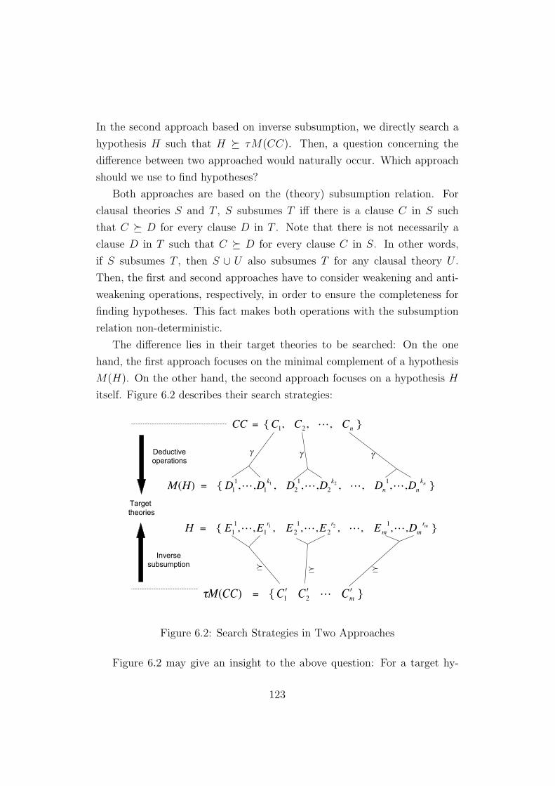
In the second approach based on inverse subsumption, we directly search a
hypothesis H such that H º τM(CC). Then, a question concerning the
difference between two approached would naturally occur. Which approach
should we use to find hypotheses?
Both approaches are based on the (theory) subsumption relation. For
clausal theories S and T , S subsumes T iff there is a clause C in S such
that C º D for every clause D in T . Note that there is not necessarily a
clause D in T such that C º D for every clause C in S. In other words,
if S subsumes T , then S ∪ U also subsumes T for any clausal theory U .
Then, the first and second approaches have to consider weakening and anti-
weakening operations, respectively, in order to ensure the completeness for
finding hypotheses. This fact makes both operations with the subsumption
relation non-deterministic.
The difference lies in their target theories to be searched: On the one
hand, the first approach focuses on the minimal complement of a hypothesis
M(H). On the other hand, the second approach focuses on a hypothesis H
itself. Figure 6.2 describes their search strategies:
!
CC = {C1, C
2, L, C
n}
!
"M(CC) = { # C 1
# C 2
L # C m}
!
!
M(H) = { D1
1,L,D
1
k1 , D2
1,L,D
2
k2 , L, Dn
1,L,D
n
kn }
!
H = { E1
1,L,E
1
r1 , E2
1,L,E
2
r2 , L, Em
1,L,D
m
rm }
Target theories
Deductiveoperations
Inversesubsumption
!
"
!
"
!
"
!
f
!
f
!
f
Figure 6.2: Search Strategies in Two Approaches
Figure 6.2 may give an insight to the above question: For a target hy-
123

pothesis H, If M(H) should be close to CC, it is sufficient to use the first
approach. Else if H should be close to τM(CC), then the second approach
is sufficient. We give the following example to describe this notation.
Example 6.2. Let a background theory B and observations E be as follows:
B = {a, b ⊃ c}. E = {d}.
Let CC be a bridge theory {a, ¬b ∨ c, ¬d}. We first assume a target
hypothesis H1 = {d ∨ b, ¬a ∨ ¬c}. τM(CC) and M(H1) are as follows:
τM(CC) = {¬a ∨ b ∨ d, ¬a ∨ ¬c ∨ d}.
M(H1) = {¬d ∨ a, ¬d ∨ c, ¬b ∨ a, ¬b ∨ c}.
Note that both CC `∗γ M(H1) and H º τM(CC) hold. However, the
number of operations for deriving the target theory is different from each
other. Using γ-operator, we can derive M(H1) from CC in such a way that
a in CC is expanded to the clause ¬b ∨ a and replaced by it and ¬d in CC
is expanded to two clauses ¬d ∨ a and ¬d ∨ c and replaced by them. Then,
the number of expanding operations should be three. On the other hand,
using inverse subsumption, we can derive H1 from τM(CC) in such a way
that the literal ¬a of the clause ¬a ∨ d ∨ b and the literal d of the clause
¬a ∨ ¬c ∨ d are dropped. Then, the number of dropping operations should
be two. Accordingly, in terms of this target hypothesis, it would be sufficient
to use inverse subsumption, since the number of operations is lower.
We next assume another target hypothesis H2 = {¬a∨ b, ¬c∨d, ¬c∨ b}.M(H2) is then {a ∨ c, ¬b ∨ c, ¬b ∨ ¬d}. Note that CC `∗
γ M(H2) and
H2 º τM(CC) hold. Using γ-operator, M(H2) is derived from CC in such
a way that two clauses a and ¬d in CC are expanded to the clause a∨ c and
the clause ¬b∨¬d, and replaced by them, respectively. Then, the number of
the expanding operations should be two. On the other hand, using inverse
subsumption, H is derived from τM(CC) in such a way that d of the clause
¬a ∨ b ∨ d and ¬a of the clause ¬a ∨ ¬c ∨ d are dropped and the clause
¬c ∨ b is added to τM(CC). The number of dropping operations should
be two. It is equal to the number of deductive operations. However, we
124
have to apply an anti-weakening operator for deriving the clause ¬c ∨ b. As
we described before, anti-weakening operators adding arbitrary clauses are
highly non-deterministic. Then, γ-operator efficiently works for deriving H2.
As we saw in this example, which approach to be used depends on the
target hypotheses. The first approach tends to derive somewhat complex
hypotheses like H2, for which we need anti-weakening operators in the case
of inverse subsumption. Note that the clause ¬c ∨ b in H2, which is derived
by an anti-weakening operator, is not necessarily used to explain E with B.
In other words, only using the other two clauses in H2, E can be explained.
Hence, the clause ¬c∨ b does not directly concern with the explanation. The
second approach with inverse subsumption is difficult to find such redun-
dant clauses that are not used to explain E. That is because we need to
ensure the consistency of the hypotheses with the background theory. Using
anti-weakening operators, we can arbitrarily add any clauses to τM(CC).
However, we have to check if the added theory is consistent with B. We may
consider that the difficulty of consistency checking is the same as the first
approach based on deductive operations. Actually, the first approach can do
it more easily.
We recall the consistency condition between B and H that B 6|= ¬H.
Since M(H) is logically equivalent to ¬H in the ground case, it is sufficient
to satisfy B 6|= M(H). If B |= M(H), Carc(B,PI) º M(H) holds. Ac-
cordingly, if Carc(B,PI) 6º M(H) should hold, H is consistent with B. By
the initial condition of bridge theories in CF-induction, any bridge theory
includes at least one instance of a clause in NewCarc(B, E,PI). We denote
by C this instance. If M(H) should keep C, then H is consistent with B,
since Carc(B,PI) 6º M(H) holds. Else, let SC be a clausal theory such that
SC ⊆ M(H) and {C} `γ SC . SC denotes the clauses obtained by applying
some γ-operator to C. If Carc(B,PI) 6º SC holds, Carc(B,PI) 6º M(H)
also holds, since M(H) contains SC . Hence, it is sufficient to take care about
the γ-operation to the clause C for the consistency of H with B. In contrast,
if we apply the same way to the second approach using inverse subsumption,
we have to additionally compute M(H) and then check if every clause in
M(H), instead of some part CS, is subsumed by a clause in Carc(B,PI).
125

From on the above consideration, the first approach with deductive op-
erations would be useful to derive active hypotheses such that refer to rules
that are not used to explain observations but are at least consistent with
the background theory. On the other hand, the second approach with in-
verse subsumption efficiently works in finding compressed hypotheses whose
description lengths tend to be short. That is because dropping operators
enable us to easily make the description length of the current theory shorter.
In the inductive learning point of view, we are used to seek more com-
pressed descriptions based on the principle of Occum’s razor. Then, the
second approach may be straightforward to this principle. In contrast, the
first approach interestingly takes the risk that hypotheses can contain some
extra rules that are not necessary to explain observations. In some cases,
this efficiently works for giving users some unexpected insights to the prior
background theory.
Example 6.3. Let a background theory B and observations E as follows:
B = {female(s) ∨ male(s)}. E = {human(s)}.
Consider a bridge theory F = {female(s) ∨ male(s), ¬human(s)}. We can
construct M(H) by applying γ-operator to F in such a way that ¬human(s)
is expanded to two clauses ¬human(s)∨female(s) and ¬human(s)∨male(s)
and replaced by them. M(H) is as follows:
{female(s) ∨ male(s), ¬human(s) ∨ female(s), ¬human(s) ∨ male(s)}.
Then, we obtain the following H by computing M(M(H)):
{¬female(s)∨human(s), ¬male(s)∨human(s), ¬female(s)∨¬male(s)}.
In addition, if we apply an anti-instantiation operator to H, we also obtain
another hypothesis represented as follows:
{female(X) ⊃ human(X), male(X) ⊃ human(X),
¬female(X) ∨ ¬male(X)}.
We notice that the last clause ¬female(X) ∨ ¬male(X) does not involve in
explaining E. Instead, it can be regarded as an integrity constraint on the
predicates female(X) and male(X) that is consistent with B.
126
6.5 Summary
In this chapter, we have studied that the generalization procedure of CF-
induction can be logically simplified while preserving its soundness and com-
pleteness. In Section 6.2, we introduced the γ-operator whose task is remov-
ing some clause D in an input clausal theory and adding a set of clauses
C1, . . . , Cn for some 0 ≤ n where each clause Ci is a super set of D. We also
showed that the γ-operator and ant-instantiation are sufficient to ensure the
completeness of CF-induction. In Section 6.3, we have proposed an alter-
native approach based on inverse subsumption with minimal complements.
Induction fields have been extended so as to describe the syntax of target hy-
potheses. We have clarified the logical relation between induction fields and
production fields that enable us to integrate inverse subsumption in Chapter
6 with generalization of CF-induction. We have also studied the issue how
bridge theories are deterministically constructed. As a result, we proposed
an incremental way to add clauses one by one to the current bridge theory.
Compared with the previous version of CF-induction, the difference is that
our proposal can deterministically construct a bridge theory and any hypoth-
esis wrt B, E and IH is derived based on the inverse subsumption, instead
of entailment. In this way, the non-determinism of CF-induction has been
logically reduced, while it ensures the soundness and completeness. In Sec-
tion 6.4, we have studied two approaches in terms of their search strategies
as well as their differences using several examples.
127

Chapter 7
Conclusions and Future Work
7.1 Summary
In this thesis, we have investigated the logical mechanism and computational
procedures in IE-based explanatory methods. Compared with other induc-
tive learning paradigms, their characteristic role lies in the applicability to
completion tasks for finding some missing facts or causal relations in the
prior knowledge. Based on this merit, we have provided a practical exam-
ple in systems biology. This motivating problem was necessary to find both
missing facts and general rules, simultaneously. Whereas significant progress
has been made in molecular biology, the prior biological inference is still in-
complete. For this situation, we have showed an inherent possibility to find
some missing rules and facts in the context of explanatory induction.
This example involves logical estimation of possible reaction states, that
is, activated or inactivated, in metabolic pathways. Like dynamic change
from fermentation to oxidation emerged in microorganisms, transitions of
highly-activated (master) reactions affect the emergence of phenotype. For
analyzing those reaction states, we introduced a logical model that describes
some of biological relations, and then use the ILP setting to estimate reac-
tion states with respect to the logical model. The initial experimental result
showed that CF-induction could realize an advanced inference simultaneously
integrating both abduction and induction. On the one hand, abductive in-
ference was used to estimate possible reaction states. On the other hand,
128
induction was used to complete missing general rules in the prior theory. In
the initial experiment, we have shown that CF-induction could find complex
hypotheses involving in both estimation and completion tasks.
Unlike the other IE-based ILP methods, CF-induction is sound and com-
plete for finding hypotheses in full clausal theories. CF-induction consists of
two non-deterministic procedures: The first one is construction of bridge the-
ories and the second is generalization into hypotheses. These two procedures
are commonly used in the modern IE-based methods, and each one constructs
a bridge theory and generalizes into hypotheses in its own way. In terms of
the generalization relation, methods like CF-induction use the inverse rela-
tion of entailment to ensure the completeness. On the other hand, methods
like Progol are based on subsumption, instead of entailment, due to computa-
tional efficiency. However, it had not been clarified whether or not the logical
reduction from entailment to subsumption could cause some incompleteness
in generalization. For this open problem, the thesis has shown that inverse
subsumption with minimal complements can ensure the completeness in gen-
eralization. We have also investigated the case of residue complements and
pointed out their fundamental limitation that arises in the fact for a ground
clausal theory S, it does not necessarily hold R2(S) = S. In contrast, we
have shown the property of minimal complements that M2(S) = µS holds.
To treat the inverse relation of entailment, we had to deal with a variety
of generalizers each of which has many ways to be applied. This fact made
generalization highly non-deterministic. In this sense, our result can be used
to reduce the non-determinisms in IE-based methods, including CF-induction
that originally uses the inverse entailment for the generalization relation. We
then considered how the generalization procedure of CF-induction can be
logically simplified based on two approach.
The first approach uses deductive operations that enable us to directly
derive the negation of a particular hypothesis from a bridge theory. Bridge
theories of CF-induction are also constructed in manner of consequence find-
ing techniques. Hence, we may be able to regard the first approach as a spe-
cific case that deductive operations are used in deriving hypotheses as much
as possible. As a result, we have proposed a new deductive operator, called
129

γ-operator, that is sufficient to derive any negations of ground hypotheses,
and showed that a concatenation of γ-operator and anti-instantiation ensures
the soundness and completeness of generalization. The second approach uses
inverse subsumption with minimal complements. In this approach, we first
clarified the logical relation between induction fields and production fields.
Along with that, we have extended induction fields into a richer represen-
tation formalization that can describe the syntax of target hypotheses (i.e.
maximum length and number of clauses in the target hypotheses). We also
compared those two approaches for generalization of CF-induction in terms of
their search strategies as well as their characteristics using several examples.
The original CF-induction contains another non-deterministic procedure:
construction of bridge theories. Let n be the number of characteristic clauses.
Then, the possible choice points to select a bridge theory should be 2n − 1.
We have shown that without losing completeness for finding hypotheses, this
non-deterministic procedure can be simplified into a deterministic way. This
result is based on the property that for every two bridge theories CC1 and
CC2 such that CC1 ⊂ CC2, τM(CC1) º τM(CC2) holds. This property
implies that any hypothesis obtained from τM(CC1) can be derived from
τM(CC2). In brief, if Carc(B ∧ Esk,P) contains a finite number of ground
clauses {C1, . . . , Cn}, it is enough to select all those ground clauses in the
bridge theory. Due to interests of computational efficiency, the thesis has
introduced an arbitrary order over characteristic clauses, and then proposed
an incremental way to construct bridge theories.
This thesis gives logical foundations for the reduction from inverse entail-
ment to inverse subsumption. Using them, we reconstruct the non-deterministic
procedures of CF-induction into more simplified ones.
7.2 Future Work
The issue on hypothesis enumeration by CF-induction needs to be addressed
in future work. The theoretical advantage of CF-induction is to preserve the
completeness for finding hypotheses in full clausal theories. In other words,
CF-induction is the unique procedure that can enumerate all the possible
130
hypotheses. If it should become possible to enumerate the target hypotheses,
we would be able to obtain some new hypotheses in many cases. Currently,
we reach the fact that for every hypothesis H, it holds that CC `∗γ M(CC)
and H º τM(CC) for some bridge theory CC. In this connection, we
remark the issue on how to realize the generalization algorithm based on
inverse subsumption as well as γ-operator. Though we have shown that
the previous generalization can be reduced into inverse subsumption or a
specific deductive operator, we do not describe those practical algorithms
in the thesis. We then intend to develop heuristics for searching relevant
hypotheses on the subsumption lattice. It would be fruitful to investigate
ways of automatically finding which literals must be added to selected clauses
by the γ-operator. We believe that studying various restrictions of the γ-
operator may allow us to systematically compare the generalisation power
of previously proposed operators. Besides, we have introduced the notion of
induction fields to efficiently focus on the target hypotheses that users wish
to obtain. As we discussed in Section 5.5, in the specific case that target
hypotheses are ground and minimal, arbitrary hypothesis can be obtained
by applying only dropping operators. Accordingly, it would be possible to
enumerate the hypotheses using dropping operators at least with brute force.
Other important future work is efficient algorithms for computing min-
imal complements. Computation of the minimal complement is equivalent
to enumeration of the minimal hitting sets, as we have shown in Chapter 2.
Though this task is solvable in quasi-polynominal time (In brief, nO(log2n))),
in case that a given induction field contains a lot of complementary literals,
the computational cost should not be ignorable. Because the number of tau-
tological clauses added to a bridge theory becomes large. This problem is
related to how relevant induction fields can be considered in advance. Progol
systems use the notion of mode declarations to describe the head and body
literals. Thus, it would be fruitful how mode declarations can be translated
into the notion of induction fields. In computational efficiency point of view,
it would be convenient to assume such an induction field where the number
of complementary literals is as small as possible. It is interesting to consider
why we have to add tautological clauses that never affect in the semantics.
131

When we look back on the examples in the thesis, its role tends to invent
some unknown predicates that never appear in the prior knowledge. For
instance, in Example 3.3, neither arc(b, c) nor ¬arc(b, c) appear in B and
E. Despite that, we allow ourself to includes two complementary literals
arc(b, c) and ¬arc(b, c) in the induction field.
It would be worth considering the issue on hypotheses evaluation that
was not sufficiently described in the thesis. In general, possible hypotheses
are not unique. In other word, there are a lot of logical theories that satisfy
the two conditions of explanatory induction However, most of the previously
proposed systems output the unique hypothesis according to their own spec-
ifications. Some adherent of pragmatism may counter as follows: It will be
sufficient that the system can find a certain valid hypothesis at some point.
It is thus practically difficult especially for the situations that need highly
expensive experiments to sequentially test the current hypothesis one by one.
In terms of abduction, SOLAR can automatically compute the subsumption-
minimal abductive hypotheses. There is a recent work [28] to statistically
evaluate those abductive hypotheses by SOLAR. Then, it would be worth
considering how CF-induction can enumerate the target inductive hypotheses
and evaluate them like SOLAR.
132

Bibliography
[1] E. Almaas, B. Kovacs, B. Vicsek, Z. N. Oltvai and A. Barabasi. Global
organization of metabolic fluxes in the bacterium escherichia coli. Na-
ture, 427(6977):839–843, 2004.
[2] D. Avis and K. Fukuda. Reverse search for enumeration. Discrete Ap-
plied Mathematics, 65(1-3):21–46, 1996.
[3] L. Badea. A refinement operator for theories. In Proc. of the 11th Int.
Conf. on Inductive Logic Programming, volume 2157 of LNCS, pages
1–14. Springer, 2001.
[4] R. Banerji. A language for the description of concepts. General Systems,
9:135–141, 1964.
[5] M. Bramer. Principles of Data Mining. Springer, 2007.
[6] J. Carbonell, editor. Machine learning paradigms and methods. 1990.
[7] C. Chang and R. Lee. Symbolic Logic and Mechanical Theorem Proving.
Academic Press, INC., 1987.
[8] K. Clark. Negation as failure. In H. Gallaire and J. Minker, editors,
Logic and Data Bases, pages 119–140, 1978.
[9] P. Cox and T. Pietrzykowski. A complete, nonredundant algorithm
for reversed skolemization. Theoretical Computer Science, (3):239–261,
1984.
[10] M. Davis and H. Putnam. A computing procedure for quantification
theory. the ACM, 7:201–215, 1960.
133

[11] Y. Deville, D. Gilbert, J. van Helden and S. Wodak. An overview of data
models for the analysis of biochemical pathways. Briefings in Bioinfor-
matics, (4):246–259, 2003.
[12] A. Doncescu, K. Inoue and T. Sato. Hypothesis-finding in systems bi-
ology. The ALP Newsletter, 21(1-3), 2008.
[13] A. Doncescu, K. Inoue and Y. Yamamoto. Knowledge-based discovery in
systems biology using CF-induction. In New Trends in Applied Artificial
Intelligence: Proc. of the 20th Int. Conf. on Industrial, Engineering
and Other Applications of Applied Intelligence Systems, volume 4570 of
LNAI, pages 395–404. Springer, 2007.
[14] A. Doncescu, Y. Yamamoto and K. Inoue. Biological systems analy-
sis using inductive logic programming. In Proc. of the 21st Int. Conf.
on Advanced Information Networking and Applications, pages 690–695.
IEEE Computer Society, 2007.
[15] T. Eiter and G. Gottlob. Hypergraph transversal computation and re-
lated problems in logic and AI. In Proc. of 8th European Conf. on Logics
in Artificial Intelligence, volume 2424 of LNCS, pages 549–564. Springer,
2002.
[16] T. Eiter and K. Makino. Abduction and the dualization problem. In
Proc. of 6th Int. Conf. on Discovery Science, volume 2843 of LNCS,
pages 1–20. Springer, 2003.
[17] T. Either, K. Makino and G. Gottlob. Computational aspects of
monotone dualization: a brief survey. Discrete Applied Mathematics,
156:2035–2049, 2008.
[18] S. Feferman et al., editor. Godel’s collected works. Oxford University
Press, 1980.
[19] M. Fredman and L. Khanchiyan. On the complexity of dualization of
monotone disjunctive normal forms. Algorithms, 21:618–628, 1996.
134

[20] E. Gold. Language identification in the limit. Information and Control,
10:447–474, 1967.
[21] E. Gregoire and L. Sais. Inductive reasoning is sometimes deductive. In
ECAI-96 Workshop on Abductive and Inductive Reasoning.
[22] N. Helft. Induction as nonmonotonic inference. In Proc. of the 1st
Int. Conf. on Principles of Knowledge Representation and Reasoning,
volume 7, pages 149–156, 1989.
[23] D. Hume. A treatise of human nature. Dover Philosophical Classics.
Dover Publications, Inc., 1739.
[24] K. Inoue. Principles of abduction. Japanese Society for Artificial Intel-
ligence, 7(1):48–59, 1991.
[25] K. Inoue. Linear resolution for consequence finding. Artificial Intelli-
gence, 56(2-3):301–353, 1992.
[26] K. Inoue. Induction as consequence finding. Machine Learning,
55(2):109–135, 2004.
[27] K. Inoue and H. Saito. Circumsciption policies for induction. In Proc.
the 14th Int. Conf. on Inductive Logic Programming, volume 3194 of
LNAI, pages 164–179. Springer, 2004.
[28] K. Inoue, T. Sato, M. Ishihata, Y. Kameya and H. Nabeshima. Evaluat-
ing abductive hypotheses using an EM algorithm on BDDs. In Proc. of
the 21st Int. Joint Conf. on Artificial Intelligence, pages 810–815, 2009.
[29] K. Iwanuma, K. Inoue, and K. Satoh. Completeness of pruning methods
for consequence finding procedure SOL. In B. P. and Z. H., editors, Proc.
of the Third Int. Workshop on First-Order Theorem Proving, pages 89–
100, 2000.
[30] M. Kanehisa and S. Goto. KEGG: Kyoto encyclopedia of genes and
genomes. Nucleic Acids Research, 28:27–30, 2000.
135
[31] T. Kimber, K. Broda and A. Russo. Induction on failure: learning con-
nected horn theories. In Proc. of Logic Programming and nonmonotonic
reasoning, Lecture Notes in Computer Science, pages 168–181, 2009.
[32] R. King, K. Whelan, F. Jones, P. Reiser, C. Bryant, S. Muggleton,
D. Kell and S. Oliver. Functional genomic hypothesis generation and
experimentation by a robot scientist. Nature, 427:247–252, 2004.
[33] N. Lachiche. Abduction and induction from a non-monotonic reasoning
perspective. In P. A. Flach and A. C. Kakas, editors, Abduction and
Induction: Essays on their relation and integration, 2000.
[34] P. Laird. Learning from good and bad data. Kluwer Acamedic Publishers,
1988.
[35] J. Larson and R. Michalski. Inductive inference of VL decision rules.
In Proc. of the Workshop in Pattern-Directed Inference Systems, pages
38–44, 1977.
[36] N. Lavrac and S. Dzeroski. Inductive logic programming: techniques and
applications. 1994.
[37] C. Lee. A completeness theorem and computer program for finding theo-
rems derivable from given axioms. PhD thesis, Dept. of Electronic Eng.
and Computer Sci., Univ. of California, Berkeley, CA, 1967.
[38] J. Lloyd. Foundations of logic programming. Springer, second edition,
1987.
[39] J. McCarthy. Circumscrition-a form of nonmonotonic reasoning. Artifi-
cial Intelligence, 13:27–39, 1980.
[40] P. Mendes and D. Kell. Non-linear optimization of biochemical path-
ways: applications to metabolic engineering and parameter estimation.
Bioinformatics, 14:869–883, 1998.
136

[41] H. Midelfart. A bounded search space of clausal theories. In Proc. of the
9th Int. Conf. on Inductive Logic Programming, volume 1634 of LNAI,
pages 210–221. Springer, 1999.
[42] T. Mitchell. Version spaces: an approach to concept learning. PhD
thesis, Stanford University, 1978.
[43] S. Muggleton. Inductive logic programming. New Generation Comput-
ing, 4(8):295–318, 1991.
[44] S. Muggleton. Inverse entailment and Progol. New Generation Comput-
ing, 13(3-4):245–286, 1995.
[45] S. Muggleton. Scientific knowledge discovery using inductive logic pro-
gramming. In Communications of the ACM, volume 42, pages 42–46,
1999.
[46] S. Muggleton and C. Bryant. Theory completion using inverse entail-
ment. In Proc. of the 10th Int. Conf. on Inductive Logic Programming,
volume 1866 of LNAI, pages 130–146, 2000.
[47] S. Muggleton and W. Buntine. Machine invention of first order predi-
cates by inverting resolution. In Proc. of the 5th Int. Conf. on Machine
Learning, pages 339–352, 1988.
[48] S. Muggleton and L. de Raedt. Inductive logic programming: theory
and methods. Logic Programming, 19/20:629–679, 1994.
[49] S. Muggleton and C. Feng. Efficient induction of logic programs. Induc-
tive Logic Programming. Academic Press, 1988.
[50] S. Muggleton, R. King and M. Sternberg. Protein secondary structure
prediction using logic-bsed machine. Protein Engineering, 5(7):647–657,
1992.
[51] H. Nabeshima, K. Iwanuma and K. Inoue SOLAR: A consequence find-
ing system for advanced reasoning. In Proc. of TABLEAUX 2003, vol-
ume 2796 of LNAI, pages 257–263. Springer, 2003.
137

[52] S. Nienhuys-Cheng and R. de Wolf. Foundations of inductive logic pro-
gramming, volume 1228 of LNCS. Springer, 1997.
[53] C. Peirce. Elements of logic, volume 2 of Collected Papers of Charles
Sanders Peirce. Harvard University Press, 1932.
[54] G. Plotkin. Automatic methods of inductive inference. PhD thesis,
Edinburgh University, 1971.
[55] G. Plotkin. A further note on inductive generalization. Machine Intel-
ligence, 6:101–124, 1971.
[56] G. Plotkin. A powerdomain construction. SIAM Journal of Computing,
5:452–497, 1976.
[57] J. Quinlan. Discovering rules from large collections of examples: a case
study. Expert Systems in the Micro electronic Age, pages 168–201, 1979.
[58] J. Quinlan. Learning logical definitions from relations. Machine Learn-
ing, 5:239–266, 1990.
[59] O. Ray. Hybrid Abductive Inductive Learning. PhD thesis, The Univer-
sity of London and the Diploma of Imperial College, 2005.
[60] O. Ray. Nonmonotonic abductive inductive learning. Applied Logic,
7:329–340, 2009.
[61] O. Ray, K. Broda and A. Russo. Hybrid abductive inductive learning:
a Generalisation of Progol. In Proc. of the 13th Int. Conf. on Inductive
Logic Programming, volume 2835 of LNAI, pages 311–328. Springer,
2003.
[62] O. Ray and K. Inoue. A consequence finding approach for full clausal
abduction. In Proc. of the 10th Int. Conf. on Discovery Science, volume
4755 of LNAI, pages 173–184. Springer, 2007.
[63] O. Ray and K. Inoue. Mode directed inverse entailment for full clausal
theories. In Revised and selected papers from the 17th Int. Conf. on
138

Inductive Logic Programming, volume 4894 of LNAI, pages 225–238,
2007.
[64] J. Robinson. A machine-oriented logic based on the resolution principle.
JACM, 12(1):23–41, 1965.
[65] S. Russell and P. Norvig. Artificial intelligence a modern approach.
Pearson Education, Inc., 2003.
[66] C. Sakama and K. Inoue. Brave induction. In Proc. the 18th Int. Conf.
on Inductive Logic Programming, volume 5194 of LNAI, pages 261–278.
Springer, 2008.
[67] C. Sammut and R. Banerji. Learning concepts by asking questions.
Machine learning: an artificial intelligence approach, 2:167–192, 1986.
[68] K. Satoh and T. Uno. Enumerating maximal frequent sets using irredun-
dant dualization. In Proc. of the 6th Int. Conf. on Discovery Science,
volume 2843 of LNCS, pages 256–268, 2003.
[69] C. Schilling, D. Letscher and B. Palsson. Theory for the systemic defini-
tion of metabolic pathways and their use in interpreting metabolic func-
tion from a pathway-oriented perspective. Theoretical Biology, 203:229–
248, 2000.
[70] K. Schugerl and K. Bellgardt. Bioreaction engineering: modeling and
control. Springer, 2000.
[71] S. Schuster, D. Fell and T. Dandekar. A general definition of metabolic
pathways useful for systematic organization and analysis of complex
metabolic networks. Nature Biotechnology, 18:326–332, 2000.
[72] E. Shapiro. Algorithmic program debugging. PhD thesis, Yale University,
1983.
[73] E. Shortliffe and B. Buchanan. A model of inexact reasoning in medicine.
Mathematical Biosciences, 23:351–379, 1975.
139

[74] G. Stephanopoulos, A. Aristidou and J. Nielsen. Metabolic engineering.
Academic Press, 1998.
[75] A. Tamaddoni-Nezhad and S. Muggleton. The lattice structure and
refinement operators for the hypothesis space bounded by a bottom
clause. Machine Learning, 76:37–72, 2009.
[76] A. Tamaddoni-Nezhad, R. Chaleil and S. Muggleton. Application of
abductive ilp to learning metabolic network inhibition from temporal
data. Machine Learning, 65:209–230, 2006.
[77] A. Turing and M. Woodger. The automatic computing engine. 1947.
[78] T. Uno. A practical fast algorithm for enumerating minimal set cover-
ings. IPSJ SIG Notes, 29:9–16, 2002.
[79] L. Valiant A theory of the learnable. Communications of the ACM,
27(11):1132–1142, 1984.
[80] P. van der Laag. An analysis of refinement operators in inductive logic
programming. PhD thesis, Erasmus Universiteit Rotterdam, 1995.
[81] A. Varma and B. Palsson. Metabolic flux balancing: basic concepts,
scientific and practical use. Nature Biotechnology, 12:994–998, 1994.
[82] A. Yamamoto. Which hypotheses can be found with inverse entailment?
In Proc. of the 7th Int. Conf. on Inductive Logic Programming, volume
1297 of LNCS, pages 296–308, 1997.
[83] A. Yamamoto. Hypothesis finding based on upward refinement of residue
hypotheses. Theoretical Computer Science, 298:5–19, 2003.
[84] A. Yamamoto and B. Fronhofer. Hypotheses finding via residue hy-
potheses with the resolution principle. In Proc. of the 11th Int. Conf.
on Algorithmic Learning Theory, volume 1968 of LNAI, pages 156–165.
Springer, 2000.
140
[85] Y. Yamamoto and K. Inoue. An efficient hypothesis-finding system im-
plemented with deduction and dualization. In Proc. of the 22nd Work-
shop on Logic Programming, pages 92–103. University Halle-Wittenberg
Institute of Computer Science Technical Report, 2008.
[86] Y. Yamamoto, K. Inoue and A. Doncescu. Estimation of possible reac-
tion states in metabolic pathways using inductive logic programming. In
Proc. of the 22nd Int. Conf. on Advanced Information Networking and
Applications, pages 808–813. IEEE Computer Society, 2008.
[87] Y. Yamamoto, K. Inoue and A. Doncescu. Abductive reasoning in can-
cer therapy. In Proc. of the 23rd Int. Conf. on Advanced Information
Networking and Applications, pages 948–953. IEEE Computer Society,
2009.
[88] Y. Yamamoto, K. Inoue and A. Doncescu. Integrating abduction and
induction in biological inference using CF-induction. In Elements of
Computational Systems biology, Wiley Book Series on Bioinformatics,
pages 213–234. John Wiley and Sons, Inc., 2009.
[89] Y. Yamamoto, K. Inoue and K. Iwanuma. Hypothesis enumeration by
CF-induction. In Proc. of the 6th Workshop on Learning with Logics
and Logics for Learning, pages 80–87. The Japanese Society for Artificial
Intelligence, 2009.
[90] Y. Yamamoto, K. Inoue and K. Iwanuma. From inverse entailment to
inverse subsumption. In Proc. of the 20th Int. Conf. on Inductive Logic
Programming, 2010.
[91] Y. Yamamoto, O. Ray and K. Inoue. Towards a logical reconstruction
of CF-induction. In Proc. of the 4th Int. Workshop on Learning with
Logics and Logics for Learning, pages 18–24. The Japanese Society for
Artificial Intelligence, 2007.
[92] Y. Yamamoto, O. Ray and K. Inoue. Towards a logical reconstruction of
CF-induction. In Satoh K., Inokuchi A., Nagao K., and Kawamura T.,
141

editor, New Frontiers in Artificial Intelligence: JSAI 2007 Conference
and Workshop Revised Selected Papers, volume 4914 of LNAI, pages
330–343. Springer, 2008.
[93] B. Zupan, I. Bratko, J. Demsar, J. Beck, A. Kuspa and G. Shaulsky.
Abductive inference of genetic networks. In 8th Conf. on AI in Medicine
in Europe, volume 2101, pages 304–313, 2001.
[94] B. Zupan, J. Demsar, I. Bratko, P. Juvan, J. Halter, A. Kuspa and G.
Shaulsky. Genepath: a system for automated construction of genetic
networks from mutant data. Bioinformatics, pages 383–389, 2003.
142