Data Min Knowl Disc Classiﬁcation of high-dimensional

unco

rrec

ted

proo

f

Data Min Knowl DiscDOI 10.1007/s10618-017-0500-7

Classification of high-dimensional evolving data streams

via a resource-efficient online ensemble

Tingting Zhai1 · Yang Gao1·

Hao Wang1· Longbing Cao2

Received: 30 March 2016 / Accepted: 27 February 2017© The Author(s) 2017

Abstract A novel online ensemble strategy, ensemble BPegasos (EBPegasos), is pro-1

posed to solve the problems simultaneously caused by concept drifting and the curse2

of dimensionality in classifying high-dimensional evolving data streams, which has3

not been addressed in the literature. First, EBPegasos uses BPegasos, an online ker-4

nelized SVM-based algorithm, as the component classifier to address the scalability 15

and sparsity of high-dimensional data. Second, EBPegasos takes full advantage of the6

characteristics of BPegasos to cope with various types of concept drifts. Specifically,7

EBPegasos constructs diverse component classifiers by controlling the budget size of8

BPegasos; it also equips each component with a drift detector to monitor and evaluate9

its performance, and modifies the ensemble structure only when large performance10

degradation occurs. Such conditional structural modification strategy makes EBPega-11

sos strike a good balance between exploiting and forgetting old knowledge. Lastly,12

we first prove experimentally that EBPegasos is more effective and resource-efficient13

than the tree ensembles on high-dimensional data. Then comprehensive experiments14

Responsible editor: Thomas Gärtner, Mirco Nanni, Andrea Passerini and Céline Robardet.

B Yang [email protected]

Tingting [email protected]

Hao [email protected]

Longbing [email protected]

1 State Key Laboratory for Novel Software Technology, Nanjing University, Nanjing, China

2 Advanced Analytics Institute, University of Technology Sydney, Sydney, Australia

123

Journal: 10618-DAMI Article No.: 0500 TYPESET DISK LE CP Disp.:2017/3/17 Pages: 24 Layout: Small-X

Au

tho

r P

ro

of

http://crossmark.crossref.org/dialog/?doi=10.1007/s10618-017-0500-7&domain=pdf

http://orcid.org/0000-0002-2488-1813

unco

rrec

ted

proo

f

T. Zhai et al.

on synthetic and real-life datasets also show that EBPegasos can cope with various15

types of concept drifts significantly better than the state-of-the-art ensemble frame-16

works when all ensembles use BPegasos as the base learner.17

Keywords High dimensionality · Concept drift · Data stream classification ·18

Online ensemble19

1 Introduction20

Mining evolving data streams has attracted numerous research attention recently21

(Zliobaite et al. 2015; Krempl et al. 2014; Zliobaite and Gabrys 2014; Zhang et al.22

2014). In particular, mining high-dimensional evolving data streams is a challenging23

task, which aims to capture the latest functional relation between the observed variables24

and the target variable and then accurately predict the labels of the upcoming observed25

values. Compared with static data, streaming data has the following characteristics:26

– Infinite amount Data is potentially endless, thus storing all data for multi-pass27

processing is impractical. To process infinite data, classifiers should work in28

resource-limited environments. Typically, the space cost for saving the models29

should be independent of the number of observations.30

– High velocity Data arrives so quickly that real-time response is required. Algo-31

rithms relying on retraining new classifiers on the latest data from scratch may not32

be useful in such environments.33

In addition to the above general characteristics, data considered in this work also34

possesses the following special characteristics:35

– Concept drifting Data is not distributed independently and identically, but has36

evolving distributions (Gama et al. 2013). The relation between the observed vari-37

ables and the target variable is expected to change with time unpredictably, while38

the distribution of the observed variables may either change or remain constant.39

Concept drifts affect decision-making; to handle them well, classifiers should be40

able to forget the old data and be consistent with the most recent data.41

– High dimensionality Data is described by hundreds or thousands of attributes, such42

as in texts, images, sounds, videos, hyper-spectral data, financial data, etc. With43

so many attributes the challenge is well known as the curse of dimensionality.44

One effect is related to the scalability. Some algorithms become intractable in45

both time and space with increasing dimensionality. Another effect is connected46

with the scarcity of the available data because the number of instances required47

to represent any distribution grows exponentially with the number of attributes48

(Tomasev et al. 2014), while each concept in the stream may not contain so huge49

data in many applications. With few instances in high-dimensional space, many50

classification models are very likely to overfit the data, thereby leading to poor51

generalization performance (Pappu and Pardalos 2014).52

The above characteristics appear in many real applications. For example, in senti-53

ment classification on twitter streams (Bifet and Frank 2010), since millions of users54

utter their opinions and make comments now and then, the messages that need to be55

123


Au

tho

r P

ro

of

unco

rrec

ted

proo

f

Classification of high-dimensional evolving data streams…

processed flow infinitely and fast, meanwhile the vocabularies used to convey positive56

and negative feelings tend to evolve with different contexts. In visual object tracking57

(Liu and Zhou 2014), surveillance cameras produce a stream of images at a rate of58

many frames per second. With the variation of illumination or background in adjacent59

frames, both the features used to describe target and non-target objects change, the60

same as the class boundary. In a personalized email filtering system (Katakis et al.61

2009), a user receives a stream of emails over time. Whether an email is a spam62

depends on the user’s interest, which may drift from time to time. In all the above63

scenarios, data is related to high dimensionality.64

Although many methods have been proposed for data stream classification, they65

generally focus on dealing with either concept drifting or high dimensionality. Few66

works consider both of them. Methods handling only concept drifting of stream-67

ing data can be classified as single-model and multi-model approaches (Hosseini68

et al. 2015). Single-model approaches are mainly incremental counterparts of con-69

ventional batch learning methods, equipped with certain strategies for coping with70

concept drifts. For example, methods based on decision trees (Gama et al. 2006; Bifet71

et al. 2010c; Rutkowski et al. 2013), k-nearest neighbors (Bifet et al. 2013), and sup-72

port vector machines (SVM) (Wang et al. 2012) have been respectively explored.73

Multi-model approaches are namely adaptive ensembles which maintain multiple74

incremental models in memory for making combined decisions. Compared with sin-75

gle models, ensemble methods are more popular since they can easily forget outdated76

data and adapt to the most recent data simply by removing outdated component clas-77

sifiers and creating new ones. Moreover, they generally have stronger generalization78

ability. There are mainly two categories of such methods (Brzezinski and Stefanowski79

2014a). The first category consists of block-based ensembles such as Learn++.NSE80

(Elwell and Polikar 2011), AUE1 (Brzezinski and Stefanowski 2011), AUE2 (Brzezin-81

ski and Stefanowski 2014b), etc., which are designed for situations where data arrives82

in batches or blocks. The second category includes online ensembles which process83

each instance once on its arrival without the requirement for storage and reprocessing.84

Representative methods are ASHTBag and ADWINBag (Bifet et al. 2009), LevBag85

(Bifet et al. 2010b), OAUE (Brzezinski and Stefanowski 2014a), DDD (Minku and Yao86

2012), etc. Among the ensembles mentioned above, Hoeffding trees (Domingos and87

Hulten 2000) are popular base learners due to the fact that, given sufficient samples,88

they are guaranteed to asymptotically approach the trees generated by batch learners.89

However, with few samples in each concept of the high-dimensional data streams,90

Hoeffding tree, as an incremental decision tree induction algorithm, tend to overfit.91

There is much less work on handling high dimensionality of data streams. Aggar-92

wal and Yu (2008) developed an instance-centered subspace classification approach,93

which constructs discriminative subspaces specific to the locality of the particular test94

instance and makes decisions by combining the results of different subspace samples.95

Wang et al. (2014) proposed a framework of sparse online classification, which over-96

comes the scalability problem by introducing sparsity in learnt weights. McCallum97

et al. (1998) considered two different naive bayes models for document classification.98

These methods, however, are not designed to handle concept drifts.99

In addition to the above methods, some improved random forests are reported to100

perform well on very high-dimensional data (Do et al. 2010; Ye et al. 2013). These101

123


Au

tho

r P

ro

of

unco

rrec

ted

proo

f

T. Zhai et al.

methods, however, cannot easily modified to be online methods. There are also some102

works focusing on building the online version of random forests. Some of them, e.g.,103

(Denil et al. 2013; Lakshminarayanan et al. 2014), are not designed to handle concept104

drifts. Some others are aware of concept drifts, but rely on certain prior knowledge,105

e.g., the range of each attribute (Abdulsalam et al. 2007; Saffari et al. 2009; Abdulsalam106

et al. 2011), which do not fit our online environment requirement that the information107

related to the data needs to be calculated or evaluated online rather than be known in108

advance. Moreover, whether these methods are robust to very high-dimensional data109

are also unknown.110

In this paper, we simultaneously tackle concept drifting and high dimensionality111

in mining streaming data. First, in order to weaken the effect caused by the curse of112

dimensionality, we apply BPegasos (Wang et al. 2012), an online kernelized SVM113

method, as the component classifier of ensemble. Second, to better handle various114

types of concept drifts, a new specialized ensemble strategy is designed for BPegasos.115

BPegasos is selected owing to the following reasons:116

1. BPegasos has good scalability. It works in O(Bd) space and its time cost for117

processing one instance is O(Bd), where d is the number of attributes, and B, of118

which the value is independent of d, is the budget for controlling the number of119

support vectors. By introducing the predefined parameter B, BPegasos can control120

the resource consumption according to the actual requirement, which makes it121

memory-efficient.122

2. BPegasos inherits the theoretical advantages of SVM so that it can generalize123

well on small data in high-dimensional space by capacity control through margin124

maximization (Abe 2005; Pappu and Pardalos 2014). The high dimensionality of125

the feature spaces induced by Mercer kernels is even considered as a bonus since126

it allows to build more powerful classifiers.127

While single BPegasos possesses the above merits, it is limited in handling various128

types of concept drifts. Meanwhile, existing ensemble strategies have mainly been129

designed for the tree classifiers, which are very different from BPegasos in stability130

and adaptability. Hence, directly applying these strategies to BPegasos may produce131

unsatisfactory results. Therefore, we design a new ensemble method for BPegasos to132

compensate for the above constraints.133

Our main contributions are threefold:134

1. We formalize the problem of online classification on data streams embedded with135

both high dimensionality and concept drifts. To the best of our knowledge, this136

problem has not been addressed in the literature.137

2. A novel solution for the above problem is developed. The solution uses BPegasos138

as the online component classifier, injects diversity among components by con-139

trolling their budget sizes, and modifies the ensemble structure by taking the data140

characteristics into account.141

3. Extensive experiments are conducted and demonstrate that our solution is superior142

to the typical Hoeffding tree-based ensembles in addressing the proposed problem.143

The superiority lies not only in accuracy but also in the resource-efficiency in144

terms of time and space. When the competitor ensembles also use BPegasos as145

123


Au

tho

r P

ro

of

unco

rrec

ted

proo

f


Table 1 Notation

Symbols Description

xt ∈ Rd , yt ∈ R A sample and its label at time t

ct : Rd → R The true concept at time t

Pt A fixed distribution at time t

base learners, our solution still shows the best capability to deal with various types146

of drifts.147

The organization of this paper is as follows. Section 2 presents the problem defini-148

tion and related work. Section 3 introduces BPegasos. Our proposed ensemble strategy149

is presented in detail in Sect. 4. Experiments are conducted and the corresponding150

results are analyzed in Sect. 5. Finally, Sect. 6 draws conclusions and discusses future151

work.152

2 Problem definition and related work153

2.1 Problem definition154

Here, we define the problem of classifying high-dimensional evolving data streams.155

For readability, Table 1 summarizes the main notation used in this paper. Assume 2156

that only one instance is available at one time and data arrives sequentially in the157

following way: {(x1, y1), (x2, y2), . . . , (xt , yt ), . . .}, where xt is drawn from distri-158

bution Pt and yt = ct (xt ). In our case, the dimensionality of variables may vary159

from a few dozen to many thousands. If the concept ct keeps constant for the whole160

stream, the stream is said to be stationary; Otherwise, it contains concept drifts. Rely-161

ing on how the time-adjacent concepts change, concept drifts are often categorized162

as sudden, gradual, and incremental drifts (Gama et al. 2014; Brzezinski and Ste-163

fanowski 2014a). Sudden drifts happen when the transition between concepts take164

place within a very limited amount of time. For gradual drifts, the transition may165

last longer and during this time, the probability that examples come from the first166

concept decreases with time, but the probability that examples from the second con-167

cept increases with time. Incremental drifting refers to the case where the concept168

changes slightly but continuously; the change is often unnoticeable until sufficient169

difference is accumulated. When the data flows in, up to time t , the available instance170

sequence is {(x1, y1), (x2, y2), . . . , (xt , yt )} and the corresponding concept sequence171

is {c1, c2, . . . , ct }. Using the available instances, the task of the learner at time t is to172

obtain a good estimate ct+1 of the true concept ct+1 with the time constraint that com-173

puting ct+1 and using it for prediction must be completed before the true label yt+1174

comes and the space constraint that the learner can only use limited memory resource.175

In the long run, the learner hopes to minimize the number of wrong predictions despite176

of the type of drifts.177

123


Au

tho

r P

ro

of

unco

rrec

ted

proo

f

T. Zhai et al.

Table 2 A summary of online ensemble methods

Methods 1© 2© 3© 4© 5© 6©

OzaBag Any OL Resampling − M × ×DWM Any OL Periodically create members ED WM × √

ASHTBag Hoeffding tree Resampling + control tree size EWMA WM × ×ADWINBag Any OL Resampling ADWIN M

√ √

LevBag Any OL Resampling using Poisson(λ) ADWIN M√ √

OAUE Any OL Periodically create members MSE WM × √

DDD Any ensemble Control resampling weights PA SWM√ ×

“OL” = “online learner”; “−” = “not required”; “ED” = “exponentially decreasing”; “EWMA” = “expo-nentially weighted moving average”; “MSE”=“mean square error”; “PA”=“prequential accuracy”; “M”represents such voting mechanism: y ← arg maxy∈Y

∑ki=1 fi,y , where fi,y is the decision of i-th base

learner on the class y and fi,y ∈ {0, 1} or fi,y ∈ [0, 1]; “WM” represents: y ← arg maxy∈Y

∑ki=1 ai fi,y ,

where ai is the weight assigned to the i-th base learner; “SWM” represents that not all the components, butsome are used in the “WM’

In the literature, there exist other definitions of concept drifts which are slightly178

different from ours. In Gama et al. (2014), Gama et al. define a concept as a joint179

probability distribution p(X, y), where X is the observed variable set and y is the180

target variable. A drift happens between time t0 and t1 if ∃X : pt0(X, y) �= pt1(X, y).181

In particular, they distinguish two different types of drifts: real concept drifts and182

virtual ones. The former refer to the changes of p(y|X) either with or without changes183

in p(X) and the latter happen if only p(X) changes. It can be seen that our definition184

corresponds to real concept drifts.185

2.2 Related work186

Online ensembles proposed in recent years are summarized in Table 2. They are187

described from the following aspects: 1© component classifiers wrapped, 2© diversity188

injection methods, 3© evaluation strategy for components, 4© aggregation strategy189

for prediction, 5© whether to use drift detection mechanism and 6© whether to190

modify the ensemble structure (i.e., add new components and discard the outdated191

ones).192

OzaBag (Oza 2005) is an online version of bagging, which simulates offline boot-193

strap sampling by presenting each available instance k times to each component,194

where k ∼ Poisson(1). Such a practice is based on the observation that the probabil-195

ity that an instance is chosen for a replicate in bootstrap sampling tends to observe196

Poisson(1) distribution. Anytime decision is made either by a simple majority vot-197

ing when each component outputs a unique class label, or by finding the maximum198

class support when each component outputs an estimate of class posterior probabili-199

ties. For the lack of structural modification, it is difficult for OzaBag to adapt to fast200

drifts.201

DWM (Kolter and Maloof 2007) maintains a dynamic weighted pool of compo-202

nents. It adjusts the weights of components, creates new components and removes203

123


Au

tho

r P

ro

of

unco

rrec

ted

proo

f


poorly-performing ones after processing every p instances. Each component has an204

initial weight 1. Whenever a components makes a wrong prediction, its weight will205

be discounted by β ∈ [0, 1). When a components’s weight falls below a threshold206

θ , it will be removed from the ensemble. Since each components’s weight is expo-207

nentially decreasing (ED), DWM is susceptible to noise and may discard some useful208

components incorrectly.209

ASHTBag (Bifet et al. 2009) is an ensemble tailored for Hoeffding trees, which210

adds diversity among components by bagging Hoeffding trees with different sizes. It211

uses exponentially weighted moving average (EWMA) to estimate the error of each212

tree and sets the weight of each tree inversely proportional to the square of its error.213

Like OzaBag, ASHTBag also suffers from fast drifts.214

ADWINBag (Bifet et al. 2009) incorporates the ADWIN drift detector (Bifet and215

Gavalda 2007) into OzaBag for detecting drifts and evaluating performance for struc-216

tural modification. LevBag (Bifet et al. 2010b) further enhances ADWINBag by217

increasing resampling weight using Poisson(λ) distribution. A typical value for λ is 6.218

However, this strategy makes LevBag vulnerable to noise, since the noisy instances219

are also learnt many times via resampling.220

OAUE (Brzezinski and Stefanowski 2014a) simulates the block-based ensembles221

by creating new members and discarding obsolete ones periodically. Performance222

evaluation is done by incrementally calculating the mean squared error (MSE) of each223

component classifier and a random prediction classifier on the last w examples. Like224

block-based ensembles, OAUE may encounter the stability-and-plasticity dilemma.225

On one hand, larger blocks can produce stable classifiers that react slowly to concept226

drifts. On the other hand, smaller blocks are beneficial to react to drifts quickly but227

bring unstable performance.228

DDD (Minku and Yao 2012) maintains four ensembles with different diversity229

levels. Each ensemble resamples using different Poisson (λ) distributions. The idea is230

motivated by the analysis of the impact of diversity on online ensemble learning in231

the presence of concept drifts in Minku et al. (2010). DDD uses some drift detection232

technique for monitoring the state of the stream so as to select different ensembles233

for prediction at different periods. The performance of each ensemble is evaluated234

using the prequential accuracy (PA) from the last moment of detecting a drift to235

current moment. Different from the above-mentioned ensemble methods, DDD is an236

ensemble of ensembles, thus its time and space costs are larger.237

No work has been reported on classifying high-dimensional data streams with238

concept drifting, to the best of our knowledge.239

3 BPegasos240

BPegasos (Wang et al. 2012) is an improvement over kernelized Pegasos (Shalev-241

Shwartz et al. 2011). In this section, we give a brief introduction to Pegasos and242

BPegasos both in the multi-class setting.243

Given a data stream {(xt , yt ), t = 1, 2, . . .}, where xt ∈ Rd , yt ∈ Y =244

{1, 2, . . . , C}, the multi-class decision function at time t is245

123


Au

tho

r P

ro

of

unco

rrec

ted

proo

f

T. Zhai et al.

ft (x) = arg maxi∈Y w(i)t

T

x, (1)246

where w(i)t is the i-th class-specific weight vector at time t .247

Pegasos uses stochastic gradient descent (SGD) to solve the following primal for-248

mulation of the SVM problem249

minw(1),w(2),...,w(C)

λ

2

∑

i∈Y

‖w(i)‖2 + 1

T

T∑

t=1

max{

0, 1 + w(rt )T

xt − w(yt )T

xt

},250

where rt = arg maxi∈Y,i �=yt w(i)Txt and λ is the parameter of the regularization term251

controlling the complexity of the model. At t-th round, when xt is available, Pegasos252

uses w(i)t learned before to predict its label by Eq. (1). After receiving the true label253

yt of xt , w(i)t is updated as254

w(i)t+1 = w

(i)t − ηt∇(i)

t , i = 1, 2, . . . , C, (2)255

where ηt = 1/(λt) is the learning step, and ∇(i)t belongs to the sub-gradient of the256

instantaneous objective function Pt with respect to w(i)t . Pt is defined as257

λ

2

∑

i∈Y

‖w(i)t ‖2 + max

{0, 1 + w

(rt )t

T

xt − w(yt )t

T

xt

},258

where rt = arg maxi∈Y,i �=yt w(i)t

T

xt . Plugging into Eq. (2) the expression of ∇(i)t , the259

update rule becomes260

w(i)t+1 = (1 − ληt )w

(i)t + β

(i)t xt , i = 1, 2, . . . , C,261

where262

β(i)t =

⎧⎨⎩

ηt if i = yt ,

−ηt if i = rt ,

0 otherwise.263

Through derivation, w(i)t can eventually be represented as264

w(i)t =

t−1∑

j=1

α(i)j x j ,265

where266

α(i)j = β

(i)j

t−1∏

k= j+1

(1 − ληk).267

123


Au

tho

r P

ro

of

unco

rrec

ted

proo

f


α(i)j is the contribution factor of the j-th instance to the i-th class. If α

(i)j is non-zero,268

x j is called a support vector (SV).269

When used for non-linear classification, a non-linear mapping φ can be introduced270

to map the original examples to a new higher dimensional feature space. w(i)t can be271

rewritten as272

w(i)t =

∑

j∈I(i)t

α(i)j φ(x j ), (3)273

where I(i)t is the set of indices of all SVs in w

(i)t . Since φ may be infinite dimensional,274

w(i)t cannot be represented explicitly by a vector just like in linear situations. Instead,275

an SV set St = {(α(i)j , x j ), j ∈ I

(i)t } needs to be maintained. By inserting Eq. (3) into276

Eq. (1), the decision function can be rewritten as277

ft (x) = arg maxi∈Y

∑

j∈I(i)t

α(i)j φ(x j )

Tφ(x). (4)278

In Eq. (4), the inner product can be efficiently computed as φ(x j )Tφ(x) = K(x j , x),279

where K(·) is a Mercer kernel derived from φ. As shown in Eq. (4), the time cost for280

prediction and the space cost for saving the model are both proportional to the number281

of SVs. The main problem of kernelized Pegasos is that the number of SVs may282

grows unboundedly with the number of data processed, which restricts its usage in283

resource-limited streaming environments. BPegasos is proposed to solve the problem.284

BPegasos keeps w(i)t spanned by at most B SVs, where B is a user-defined param-285

eter. Denote It =⋃C

i=1 I(i)t ; when |It | > B, a budget maintenance step is triggered286

and achieved as287

w(i)t ← w

(i)t − ∆

(i)t , i = 1, 2, . . . , C. (5)288

where ∆(i)t is the weight degradation of w

(i)t before and after the budget maintenance.289

Wang et al. (2012) proved that a good budget maintenance strategy should minimize290

the total degradation∑C

i=1 ||∆(i)t ||2. Specifically, they proposed three strategies: (i)291

deleting one SV, (ii) projecting one SV to the remaining ones, and (iii) merging two292

SVs into a newly created one. Among them, the merging strategy is the most appealing,293

since it has time and space complexity of O(Bd) per iteration and can produce smaller294

total weight degradation. The basic idea of merging is to choose two SVs and then295

merge them into a new one. The details are in Wang et al. (2012).296

Algorithm 1 presents the pseudocode of BPegasos. In the remaining sections, when297

it comes to BPegasos, we refer to the BPegasos with the merging strategy. By default,298

the popular RBF kernel with width δ is used (Hsu et al. 2003):299

K(x j , x) = exp

(−‖x j − x‖2

2δ2

).300

123


Au

tho

r P

ro

of

unco

rrec

ted

proo

f

T. Zhai et al.

Algorithm 1: BPegasosInput: Data stream D = {(xt , yt ), t = 1, 2, . . .}; budget B; regularization parameter λ; kernel

function K(·)Output: ft (x)

1 for t = 1, 2, . . . do

2 Receive xt ;3 Predict its label using Eq. (4);4 Receive the true label yt ;

5 Update w(i)t using SGD;

6 if |It | > B then

7 Do the budget maintenance using Eq. (5);

4 Ensemble BPegasos (EBPegasos)301

In order to improve the adaptability of BPegasos to various types of drifts, a novel302

online ensemble method, called EBPegasos, is proposed. In the following, three critical303

parts in EBPegasos are presented respectively:304

1. Diversity injection, which produces a component set as accurately and diversely305

as possible;306

2. Component management, which monitors the performance status of components,307

and makes accurate predictions by aggregating the outputs of the components.308

3. Structural modification, discards the components at the right time, with the objec-309

tive of striking a good balance between exploiting and forgetting old knowledge.310

4.1 Diversity injection311

It is known that diversity plays an important role in learning data streams with concept312

drifts (Minku et al. 2010). For unstable learners such as decision trees, small changes313

in data can bring about large variations in the classification. Accordingly, resampling314

is effective for increasing diversity among unstable learners. Unfortunately, as an315

SVM-based method, BPegasos is relatively stable and thus resampling cannot help316

much.317

Instead of using resampling, EBPegasos creates diversity by allowing different318

budget sizes of BPegasos components. This is due to the fact that varying the budget319

size greatly affects the performance of BPegasos (Wang et al. 2012). In general, a320

larger budget means more stable performance since the margin information is better321

kept by more SVs. This is preferable when the data stream is stable, as BPegasos322

may thus reduce the number of false alarms of concept drifting. However, the stability323

becomes an impediment to BPegasos when the underlying concept in the data stream324

is actually drifting, as it usually takes more time for BPegasos to forget that many325

obsolete SVs. In contrast, a smaller budget means higher instability of performance326

but more sensitivity to changes, which thus may cause more false alarms when the327

data stream is stable but contribute to the early detection of concept drifts when they328

indeed happen. Considering this, we design EBPegasos to include multiple BPegasos329

123


Au

tho

r P

ro

of

unco

rrec

ted

proo

f


classifiers with different budget sizes, so that it can achieve good performance in both330

stable and unstable periods of the data stream.331

4.2 Component management332

EBPegasos predicts by weighted majority voting. In particular, when making a predic-333

tion yt for the data sample xt , EBPegasos calculates a weighted sum of the predictions334

of the components,335

yt ← arg maxy∈Y

k∑

i=1

ait · I

(f it (xt ) = y

), (6)336

where ait is the weight assigned to the i-th component, and I(·) is an indicator function337

which outputs 1 if the Boolean expression in the brackets is true, or 0 otherwise.338

To obtain ait , EBPegasos equips each of its components with an ADWIN (Bifet and339

Gavalda 2007) to monitor and evaluate its performance. ADWIN is originally designed340

as a drift detector; Fig. 1 presents its working process. Every time a component makes341

a prediction yt , a single bit b is generated (via comparing yt to yt , the true class label342

of xt ) and fed into ADWIN, indicating whether the prediction yt is correct (b = 0) or343

wrong (b = 1). As shown in Fig. 1a, ADWIN tracks a window W of such bits, which344

consists of two large enough sub-windows W0 and W1. The basic idea of ADWIN is345

that, when there is no concept drift in the data stream, the average of the elements346

(i.e., the error rate) in W0 should be statistically consistent with the average in W1.347

Put in other words, whenever the difference between the error rates in W0 and W1 is348

statistically significant, ADWIN alarms a concept drift, in which case ADWIN drops349

the sub-window W0 and makes W1 a new W (Fig. 1b). Note that the overall error rate350

in W (i.e., the number of 1’s in W divided by the length of W ), Errit , can be used as a351

performance measure of the corresponding component. Hence, the weight ait can be352

computed as353

ait = 1 − Erri

t∑ki=1(1 − Erri

t ), i = 1, 2, . . . , k,354

where k is the number of ensemble members.355

00010010010 011010110101

W0 W1

W

1

(a)

00010010010 011010110101

W0 W1

W

1

(b)

Fig. 1 The working process of ADWIN. a W before a drift, b W after a drift

123


Au

tho

r P

ro

of

unco

rrec

ted

proo

f

T. Zhai et al.

As mentioned in Sect.4.1, there are component BPegasos classifiers with various356

budgets in EBPegasos. Hence, another benefit of such a practice is that the ADWIN357

detectors associated with different budgeted classifiers can issue alarms at different358

times, which helps to reduce the false negative (missing alarms) rate of the drift359

detection.360

4.3 Conditional structural modification361

Structural modification involves when to create new components to substitute the362

outdated ones. To handle various types of drifts well, especially for fast incremental363

drifts, structural modification is essential in ensemble methods.364

Existing ensemble methods such as ADWINBag and LevBag modify the structure365

once a drift is detected. However, since these methods are designed for component366

classifiers without forgetting mechanisms, their timing of making the structural modi-367

fication is not suitable for BPegasos. BPegasos is very different from other component368

classifiers used in other ensemble solutions in that it naturally has slow forgetting369

capability due to its budget maintenance. Specifically, when drifts occur, BPega-370

sos has two ways to establish the new decision margin: (i) discarding the previous371

model learnt and retraining a new one on the most recent data; or (ii) keeping372

updating the previous model incrementally. Which way is better depends on the373

intrinsic characteristics of data. Intuitively, the first way is better for severe drifts374

that bring large performance degradation of classifiers; while for slight drifts that375

bring small degradation and that maybe are caused by noise, the second way is376

better.377

In order to identify the severity of drifting, we define r , the model degradation rate378

(MDR), as follows:379

r = f1 − f0

|W1|, (7)380

where f0 and f1 are the errors in the sub-windows W0 and W1 in Fig. 1b respectively.381

f1− f0 reflects how much a model degrades when the concept drifts, and |W1| indicates382

how long it takes for the accumulated degradation to be detected.383

For severe drifts, one may expect a large r since performance degrades greatly in384

relatively short time. In contrast, for slight drifts, r is small since getting a significant385

degradation f1 − f0 needs a larger window W1. Intuitively, with a large r , it is better to386

forget old knowledge rapidly by retraining a new classifier from scratch; and, on the387

contrary, with a small r , exploiting fully the old knowledge by incrementally updating388

the old classifiers is often preferable. Therefore, we define a threshold θ in EBPegasos389

for determining when to use which way. Specifically, when a drift alarm is issued, if r390

is larger than θ , a new classifier is retrained; otherwise, the old classifier is retained and391

keeps updating itself. In this way, EBPegasos strikes a good balance between reusing392

and fast forgetting previously learned knowledge.393

123


Au

tho

r P

ro

of

unco

rrec

ted

proo

f


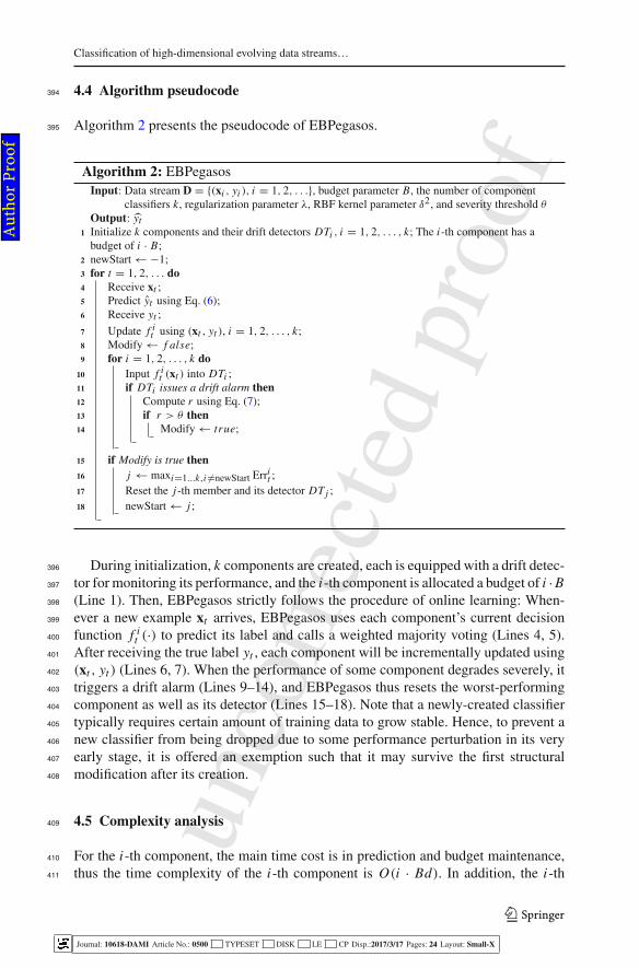
4.4 Algorithm pseudocode394

Algorithm 2 presents the pseudocode of EBPegasos.395

Algorithm 2: EBPegasosInput: Data stream D = {(xi , yi ), i = 1, 2, . . .}, budget parameter B, the number of component

classifiers k, regularization parameter λ, RBF kernel parameter δ2, and severity threshold θ

Output: yt

1 Initialize k components and their drift detectors DTi , i = 1, 2, . . . , k; The i-th component has abudget of i · B;

2 newStart ← −1;3 for t = 1, 2, . . . do

4 Receive xt ;5 Predict yt using Eq. (6);6 Receive yt ;

7 Update f it using (xt , yt ), i = 1, 2, . . . , k;

8 Modify ← f alse;9 for i = 1, 2, . . . , k do

10 Input f it (xt ) into DTi ;

11 if DTi issues a drift alarm then

12 Compute r using Eq. (7);13 if r > θ then

14 Modify ← true;

15 if Modify is true then

16 j ← maxi=1...k,i �=newStart Errit ;17 Reset the j-th member and its detector DT j ;18 newStart ← j ;

During initialization, k components are created, each is equipped with a drift detec-396

tor for monitoring its performance, and the i-th component is allocated a budget of i · B397

(Line 1). Then, EBPegasos strictly follows the procedure of online learning: When-398

ever a new example xt arrives, EBPegasos uses each component’s current decision399

function f it (·) to predict its label and calls a weighted majority voting (Lines 4, 5).400

After receiving the true label yt , each component will be incrementally updated using401

(xt , yt ) (Lines 6, 7). When the performance of some component degrades severely, it402

triggers a drift alarm (Lines 9–14), and EBPegasos thus resets the worst-performing403

component as well as its detector (Lines 15–18). Note that a newly-created classifier404

typically requires certain amount of training data to grow stable. Hence, to prevent a405

new classifier from being dropped due to some performance perturbation in its very406

early stage, it is offered an exemption such that it may survive the first structural407

modification after its creation.408

4.5 Complexity analysis409

For the i-th component, the main time cost is in prediction and budget maintenance,410

thus the time complexity of the i-th component is O(i · Bd). In addition, the i-th411

123


Au

tho

r P

ro

of

unco

rrec

ted

proo

f

T. Zhai et al.

component stores i · B SVs, and thus requires O(i · Bd) space. Each ADWIN drift412

detector needs O(log |W |) time and O(log |W |) memory for processing an input bit,413

where W is the maximum stable window (Bifet and Gavalda 2007). Hence, checking414

whether it is necessary to do the structural modification takes O(k log |W |) time,415

dominating the time cost, O(k), for actually performing a structural modification.416

Therefore, to sum up, EBPegasos works in O(k2 Bd + k log |W |) space and costs417

O(k2 Bd + k log |W |) time per iteration.418

It is easy to see that (i) the space cost of EBPegasos remains constant after its initial419

configuration, and (ii) the time cost for processing one data instance is irrelevant to420

the length of the data stream. Hence, EBPegasos is very suitable for resource-limited421

situations.422

5 Experiments423

In this section, four sets of experiments are presented.424

1. Accuracy and efficiency analysis on high-dimensional data. This set of experiments425

demonstrates the advantages of EBPegasos over the state-of-the-art tree ensembles426

on high-dimensional data streams.427

2. Adaptivity analysis. This set of experiments compares the ability of EBPegasos to428

cope with various types of concept drifts with that of the state-of-the-art ensemble429

frameworks, showing that the superiority of EBPegasos comes from not only the430

choice of the components but also its novel component ensemble strategy.431

3. Comparative analysis on low-dimensional data. This set of experiments observes432

the performance of EBPegasos compared to the tree ensembles on low-dimensional433

datasets.434

4. Sensitivity analysis. This set of experiments analyzes the parameter sensitivity of435

EBPegasos.436

All the experiments were conducted in the Massive Online Analysis (MOA)437

framework (Bifet et al. 2010a), which is a dedicated software platform for running438

experiments of evolving data stream mining, containing most of the competitor algo-439

rithms considered in our experiments. All experiments were performed on a machine440

with 2.60GHz Intel(R) Xeon(R) CPU E5-2650 v2 and 64GB 1866MHz DDR3 mem-441

ory.442

Prequential accuracy (Gama et al. 2014, 2013) is used to evaluate the method,443

which is computed at every moment t as soon as the predicition yt is made444

Acc(t) = 1

t

t∑

i=1

L(yi , yi ),445

where L(yi , yi

)= 1 if yi = yi and 0 otherwise. For comparing two methods,446

average prequential accuracy over all the moments is reported. Since we handle447

high-dimensional data in resource-limited scenarios, space and time costs are also of448

essential importance in evaluating an algorithm. To measure them, we use the tools449

123


Au

tho

r P

ro

of

unco

rrec

ted

proo

f


Table 3 The characteristics of the datasets and the parameter settings of EBPegasos

Name Datasets EBPegasos

#inst #Attr #Classes k λ δ2 B θ

Spam_data 9324 500 2 5 1e−4 10 4 1e−5

Gisette 6000 5000 2 5 1e−4 5 80 1e−5

NewsGroup4 12,000 26,214 2 5 1e−6 60 4 1e−5

Spam_corpus 9324 39,916 2 5 1e−4 70 4 1e−5

provided in MOA. In addition, to verify whether the performance difference is statisti-450

cally significant, Wilcoxon signed-rank test (Demšar 2006) is used, which is regarded451

as the best statistical measure for evaluating two classifiers on multiple datasets.452

5.1 Accuracy and efficiency analysis on high-dimensional data453

This section aims to demonstrate the accuracy and efficiency of EBPegasos in face of454

high-dimensional data, compared with the state-of-the-art tree ensembles. Four real-455

world very high-dimensional datasets are used and their characteristics are shown456

in Table 3. Spam_corpus is from SpamAssasin data collection (Katakis et al. 2009),457

containing 9,324 emails, in which around 20% are spams. Each email is represented458

as a 39,916-dimensional vector, where each binary component indicates whether or459

not a corresponding term appears in this email. Spam_data is the dataset after applying460

feature selection with the χ2 measure on Spam_corpus (Katakis et al. 2010). The task461

of Gisette1 data is to distinguish the highly confusable handwritten “4” and “9”. Each462

record in the dataset describes such a digit. NewsGroup4, created from 20newsGroup,2463

simulates the evolution of a particular user’s interest in four news groups over time.464

The parameter settings of EBPegasos on the above datasets are chosen by using the465

first 20% of data and are displayed in Table 3. The chosen settings are then used on466

the whole stream.467

The compared methods include OzaBag (Oza) (Oza 2005), ASHTBag (ASHT)468

(Bifet et al. 2009), ADWINBag (ADWIN) (Bifet et al. 2009), LevBag (Lev) (Bifet et al.469

2010b), DWM (Kolter and Maloof 2007), OAUE (Brzezinski and Stefanowski 2014a)470

and multinominal naive bayes (MNB) (McCallum et al. 1998). The tree ensemble471

methods use 10 component classifiers, each of which is the Hoeffding Naive Bayes472

tree (HNBT) (Holmes et al. 2005) that adds Naive Bayes prediction at each leaf so473

as to adaptively choose at each leaf between majority class prediction and Naive474

Bayes prediction. In addition, we also consider one possible random forests (RF)475

implementation, which uses as the component classifier random HNBT that selects√

d476

attributes randomly (d is the number of attributes) and only uses these attributes when477

building a tree and making predicition, as Bifet et al. did in their experiments (Bifet478

1 https://www.csie.ntu.edu.tw/~cjlin/libsvmtools/datasets/binary.html#gisette.2 http://qwone.com/~jason/20Newsgroups/.

123


Au

tho

r P

ro

of

https://www.csie.ntu.edu.tw/~cjlin/libsvmtools/datasets/binary.html#gisette

http://qwone.com/~jason/20Newsgroups/

unco

rrec

ted

proo

f

T. Zhai et al.

et al. 2010b). RF combines 25 such trees using LevBag ensemble framework. Given479

that using of Hoeffding bound hinders trees from growing which may degrade their480

performance, we consider two groups of parameter settings of trees. In the first setting,481

the split confidence is 0.01 and the tie threshold is 0.05. Such setting does not allow482

attributes to split until high quasi-certainty about which attribute test should be used is483

obtained. The second setting using the tie threshold as 1.0 turns a tree into a regular tree484

that introduces an attribute splitting after seeing a relatively small and fixed number485

of instances. The grace period parameter in both settings is chosen from the interval486

[20, 30, . . . , 200]. For DWM, the factor for discounting weights and the threshold for487

deleting component classifiers are 0.5 and 0.01 respectively, as suggested in Kolter488

and Maloof (2007). But the period parameter in DWM for controlling component489

removal, creation and weight update and the window size in OAUE for structural490

modification and component evaluation are both data-specific and are chosen from491

the interval [100, 200, . . . , 1000] so that they achieves the best performance. The492

results of the tree ensembles for the two different parameter settings, including the493

average prequential accuracy, total processing time consisting of training and testing494

time, and maximum space cost have been reported respectively in Table 4, in which, “-495

” represents that the results cannot be obtained since the corresponding algorithm runs496

out of the available memory and interrupts its performing. As a specialized document497

classifier, MNB is not suitable for the Gisette data; thus its result on the dataset is498

shown as “–” in the Table 4. The results of EBPegasos are presented in the last column499

of Table 4.500

As we can see, for the tree ensembles, the second parameter setting generally leads501

to better average prequential accuracy than the first one does, but costs more time and502

space resources. Among the tree ensembles, LevBag tends to use much greater time503

and space resources, which limits its performance on very high dimensional datasets.504

RF is not always more resource-efficient than the other tree ensembles, but achieves505

significantly better accuracy in most cases. As a simple document classifier and also a506

single model, MNB is very resource-efficient. However, for lacking of the mechanism507

to handle concept drifts, its performance suffers greatly on NewsGroup4. Compared508

with all the methods on the four datasets, EBPegasos always achieves the best average509

prequential accuracy, meanwhile its memory and time cost, although larger than MNB,510

is smaller than the tree ensembles in most cases.511

5.2 Adaptability analysis512

In this section, we want to compare the adaptability of EBPegasos to that of state-of-513

the-art ensemble methods mentioned above on datasets with various types of concept514

drifts. All the ensemble algorithms use BPegasos as the component learners, thus the515

base learners in the tree-based ensembles are substituted with BPegasos.3516

3 ASHTBag is excluded here since its ensemble strategy is dedicated to Hoeffding trees.

123


Au

tho

r P

ro

of

unco

rrec

ted

proo

f


Ta

ble

4T

heav

erag

epr

eque

ntia

lacc

urac

y(%

),pr

oces

sing

tim

e(s

)an

dsp

ace

cost

(MB

)on

the

very

high

-dim

ensi

onal

data

sets

Dat

aset

sO

zaA

SH

TA

DW

INL

evD

WM

OA

UE

RF

MN

BE

BP

Spa

m_d

ata

(%)

92.0

492

.11

92.6

296

.58

93.0

990

.47

95.4

495

.77

96

.90

95.0

194

.69

95.2

996

.44

93.3

590

.89

95.6

5

(s)

16.3

017

.49

19.1

652

.55

19.0

213

.37

16.7

21

.65

11.5

2

30.0

927

.72

29.8

278

.90

26.6

519

.86

20.0

1

(MB

)28

.58

17.4

617

.61

113.

852.

2416

.21

35.1

70

.22

0.60

76.6

936

.54

52.7

620

2.40

3.29

42.2

346

.80

Gis

ette

(%)

61.2

359

.24

61.2

383

.43

62.3

965

.35

85.4

1–

87

.53

77.4

664

.42

77.4

676

.29

83.2

975

.73

83.7

1

(s)

286.

3335

3.42

342.

7170

8.64

88.3

813

2.68

141.

04–

2829

.79

489.

7754

8.52

544.

2116

71.0

18

8.0

541

8.90

311.

21

(MB

)23

0.32

158.

1223

0.34

1159

.15

48.1

784

.34

102.

76–

46

.52

988.

3146

1.64

988.

3215

24.4

912

9.29

577.

5229

0.80

New

sGro

up4

(%)

52.7

052

.03

53.8

262

.95

57.1

751

.48

76.6

075

.95

90

.49

63.5

660

.04

62.7

8-

67.1

857

.65

79.9

4

(s)

2098

. 85

2505

.74

3082

.90

6285

.23

859.

5313

35.9

826

,422

.80

2.6

866

1.61

4088

.70

4260

.18

4577

.57

-33

01.3

441

20.9

992

,935

.80

(MB

)17

69.0

418

75.4

412

09.2

520

31.0

652

1.20

1388

.44

1919

.89

2.9

715

.59

1992

.99

1916

.95

1759

.07

-19

08.7

319

91.9

414

60.8

6

Spa

m_c

orpu

s(%

)87

.52

87.3

489

.69

94.4

190

.32

87.0

592

.84

94.6

59

6.8

5

94.2

292

.44

94.1

6-

91.5

190

.02

95.3

9

(s)

1395

.10

1570

.95

1467

.71

4180

.36

2085

.22

1159

.50

22,1

43. 6

01

85

.41

902.

10

5779

.12

5613

.11

5706

.43

-45

73.8

634

93.7

464

,750

.30

(MB

)18

48.2

512

29.4

211

53.0

714

83.9

813

1.88

1249

.95

1241

.78

26

.15

45.3

6

1841

.36

1916

.07

958.

46-

278.

4816

58.0

719

19.3

5

123


Au

tho

r P

ro

of

unco

rrec

ted

proo

f

T. Zhai et al.

Table 5 The characteristics of the datasets

Datasets #inst #Attr #Classes Noise #Drift Drift type

Hy_f 1 M 50 2 10% – Incremental

Hy_s 1 M 50 2 10% – Incremental

RBF_f 100 k 100 10 – – Incremental

RBF_s 100 k 100 10 – – Incremental

LED_s 400 k 24 10 10–20–15–10% 3 Sudden

LED_g 400 k 24 10 10–20–15–10% 3 Gradual

SEA_s 400 k 3 2 10–20–15–10% 3 Sudden

SEA_g 400 k 3 2 10–20–15–10% 3 Gradual

Tree_s 400 k 30 10 – 3 Sudden

Tree_g 400 k 30 10 – 3 Gradual

Waveform_s 400 k 40 3 – 3 Sudden

Waveform_g 400 k 40 3 – 3 Gradual

Covertype 581 k 54 7 – – Unknown

Kddcup99 494 k 121 23 – – Unknown

Noise is the label noise in each concept

We first use synthetic datasets to analyze the performance of the algorithms. For517

constructing datasets with sudden, gradual and incremental drifts,4 we use the data518

stream generators available in MOA, including the Rotating hyperplane, Random RBF,519

LED, SEA, Random Tree and Waveform generators, which have been used frequently520

in the context of concept drifts (Bifet et al. 2010b; Brzezinski and Stefanowski 2011;521

Brzezinski and Stefanowski 2014a, b). Table 5 presents the characteristics of these522

datasets.523

Besides the synthetic datasets, two real datasets are also considered. The first one is524

the Covertype5 which contains the forest cover type obtained from US Forest Service525

Region 2 Resource Information System data. The second one is the kddcup99,6 which526

includes a wide range of intrusions simulated in a military network and whose task is527

to distinguish between bad connections and normal connections. We have transformed528

the original nominal attributes in Kddcup99 to binary attributes that are then treated529

as numeric.530

To perform fair comparisons, all methods use 5 BPegasos components and take531

the same total budget space B (in terms of the number of SVs) on each dataset.532

With such a resource limit, EBPegasos combines BPegasos components with budgets533

B, 2B, 3B, 4B, 5B to create diversity among components (Sect. 4.1), and guarantees534

15B = B. The other methods use BPegasos components with the same budget B ′,535

and ensures 5B ′ = B. To observe how much improvement EBPegasos can make536

4 The scripts for generating these datasets are available at http://cs.nju.edu.cn/rl/people/zhaitt/datasetsGenerateScript.txt.5 It can be downloaded from http://moa.cms.waikato.ac.nz/datasets/.6 It can be downloaded from http://www.cse.fau.edu/~xqzhu/stream.html.

123


Au

tho

r P

ro

of

http://cs.nju.edu.cn/rl/people/zhaitt/datasetsGenerateScript.txt

http://cs.nju.edu.cn/rl/people/zhaitt/datasetsGenerateScript.txt

http://moa.cms.waikato.ac.nz/datasets/

http://www.cse.fau.edu/~xqzhu/stream.html

unco

rrec

ted

proo

f


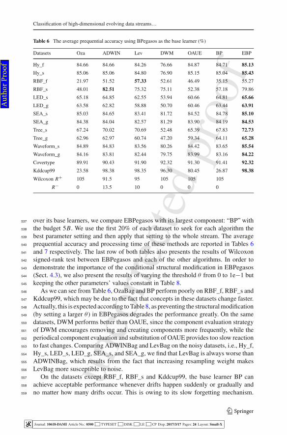
Table 6 The average prequential accuracy using BPegasos as the base learner (%)

Datasets Oza ADWIN Lev DWM OAUE BP EBP

Hy_f 84.66 84.66 84.26 76.66 84.87 84.71 85.13

Hy_s 85.06 85.06 84.80 76.90 85.15 85.04 85.43

RBF_f 21.97 51.52 57.33 52.61 46.49 35.15 55.27

RBF_s 48.01 82.51 75.32 75.11 52.38 57.18 79.86

LED_s 65.18 64.85 62.55 53.94 60.66 64.81 65.66

LED_g 63.58 62.82 58.88 50.70 60.46 63.44 63.91

SEA_s 85.03 84.65 83.41 81.72 84.52 84.78 85.10

SEA_g 84.38 84.04 82.57 81.29 83.90 84.19 84.53

Tree_s 67.24 70.02 70.69 52.48 65.39 67.83 72.73

Tree_g 62.96 62.97 60.74 47.20 59.34 64.11 65.28

Waveform_s 84.89 84.83 83.56 80.26 84.42 83.65 85.54

Waveform_g 84.16 83.81 82.44 79.75 83.99 83.16 84.22

Covertype 89.91 90.43 91.90 92.32 91.30 91.41 92.32

Kddcup99 23.58 98.38 98.35 96.30 80.45 26.87 98.38

Wilcoxon R+ 105 91.5 95 105 105 105

R− 0 13.5 10 0 0 0

over its base learners, we compare EBPegasos with its largest component: “BP” with537

the budget 5B. We use the first 20% of each dataset to seek for each algorithm the538

best parameter setting and then apply that setting to the whole stream. The average539

prequential accuracy and processing time of these methods are reported in Tables 6540

and 7 respectively. The last row of both tables also presents the results of Wilcoxon541

signed-rank test between EBPegasos and each of the other algorithms. In order to542

demonstrate the importance of the conditional structural modification in EBPegasos543

(Sect. 4.3), we also present the results of varying the threshold θ from 0 to 1e−1 but544

keeping the other parameters’ values constant in Table 8.545

As we can see from Table 6, OzaBag and BP perform poorly on RBF_f, RBF_s and546

Kddcup99, which may be due to the fact that concepts in these datasets change faster.547

Actually, this is expected according to Table 8, as preventing the structural modification548

(by setting a larger θ ) in EBPegasos degrades the performance greatly. On the same549

datasets, DWM performs better than OAUE, since the component evaluation strategy550

of DWM encourages removing and creating components more frequently, while the551

periodical component evaluation and substitution of OAUE provides too slow reaction552

to fast changes. Comparing ADWINBag and LevBag on the noisy datasets, i.e., Hy_f,553

Hy_s, LED_s, LED_g, SEA_s, and SEA_g, we find that LevBag is always worse than554

ADWINBag, which results from the fact that increasing resampling weight makes555

LevBag more susceptible to noise.556

On the datasets except RBF_f, RBF_s and Kddcup99, the base learner BP can557

achieve acceptable performance whenever drifts happen suddenly or gradually and558

no matter how many drifts occur. This is owing to its slow forgetting mechanism.559

123


Au

tho

r P

ro

of

unco

rrec

ted

proo

f

T. Zhai et al.

Table 7 The total processing time in second on each dataset, including both the training and the testingtime when using BPegasos as the base learner

Datasets Oza ADWIN Lev DWM OAUE BP EBP

Hy_f 1174.78 1327.49 1903.08 1739.7 2067.46 632.763 1976.16

Hy_s 1199.27 1307.59 1930.51 1685.65 2091.53 623.617 1958.15

RBF_f 2965.60 1537.0 1874.31 2127.24 2932.46 1239.37 2724.67

RBF_s 2832.94 1388.12 1093.24 1702.79 4169.06 1032.45 2361.08

LED_s 1336.73 1223.16 1657.17 2045.43 2384.13 844.78 2255.99

LED_g 1404.38 1290.68 1790.18 2140.01 2529.25 889.15 2580.63

SEA_s 353.71 353.00 659.03 1669.82 616.28 174.21 575.65

SEA_g 359.10 359.16 650.92 1666.93 633.83 178.58 593.64

Tree_s 1660.54 1425.31 1699.37 2206.34 2798.93 671.76 1740.63

Tree_g 1794.4 1609.78 2172.84 2355.32 2917.6 980.18 2324.46

Waveform_s 440.74 390.36 496.32 403.96 916.92 193.68 1083.61

Waveform_g 394.84 364.31 497.76 976.05 705.42 208.12 1175.66

Covertype 443.42 511.42 607.57 539.27 545.22 190.41 565.292

Kddcup99 307.21 1693.14 2465.44 1283.15 1240.11 155.66 2502.26

Wilcoxon R+ 11 0 16 35 69 0

R− 94 105 89 70 36 105

Table 8 The average prequential accuracy of EBPegasos when the threshold θ varies from 0 to 1e−1

Datasets 0 1e−6 1e−5 1e−4 1e−3 1e−2 1e−1

Hy_f 76.14 76.14 76.67 85.13 85.13 85.13 85.13

Hy_s 76.29 76.29 81.38 85.43 85.43 85.43 85.43

RBF_f 55.27 55.27 55.24 54.92 52.31 17.14 17.14

RBF_s 79.22 79.23 79.86 52.38 52.38 52.38 52.38

LED_s 61.35 61.35 64.55 65.29 65.66 65.27 65.27

LED_g 59.18 59.18 63.49 63.91 63.91 63.91 63.91

SEA_s 81.67 81.67 83.55 85.10 85.08 85.08 85.08

SEA_g 81.10 81.10 84.53 84.53 84.53 84.53 84.53

Tree_s 72.38 72.54 72.73 72.73 72.70 69.92 69.92

Tree_g 62.37 62.63 64.82 65.28 65.28 65.28 65.28

Waveform_s 84.29 84.29 84.24 85.54 69.99 69.99 69.99

Waveform_g 84.00 84.22 82.44 69.55 69.60 69.60 69.60

Covertype 92.32 92.27 92.22 92.15 91.63 90.75 90.75

Kddcup99 98.38 98.38 98.37 98.39 98.38 23.25 23.25

Ignoring of the characteristic of BPegasos, ADWINBag, LevBag, DWM and OAUE560

cannot outperform BPegasos in many cases, e.g. on LED_g, SEA_s, SEA_g and561

Tree_g. In contrast, EBPegasos, considering the characteristic, can always obtain better562

performance than BPegasos on all datasets.563

123


Au

tho

r P

ro

of

unco

rrec

ted

proo

f


For the Wilcoxon signed-rank test, the null hypothesis is that the two algorithms564

being compared can achieve equal performance. When the number of datasets is 14, if565

min{R+, R−}≤ 21, the null hypothesis can be rejected with a confidence level 0.05.566

Seen from the last row of Table 6, we can conclude that EBPegasos is statistically better567

than the other methods in terms of averaged prequential accuracy. In terms of the total568

processing time, Bpegasos, as a single learner, costs the least time on all datasets.569

Among the ensemble methods, OzaBag, ADWINBag and LevBag cost significantly570

less time than EBPegasos.571

From Table 8, we can see clearly that the function of conditional structural modi-572

fication in EBPegasos. On Hy_f, Hy_s, LED_s, LED_g, SEA_s, SEA_g and Tree_g,573

exploiting old knowledge fully by setting a larger θ is more beneficial, while on574

RBF_f, RBF_s, Tree_s, Waveform_s, Waveform_g, Covertype and Kddcup99, pro-575

moting structural modification by setting a smaller θ (thus learning new knowledge576

quickly) is better. From the above analysis, we can conclude that the conditional577

structural modification strategies (Sect. 4.3) makes EBPegasos strike a good balance578

between exploiting old knowledge fully and learning new knowledge. The appropriate579

value for θ may depend on the specific data characteristics.580

5.3 Comparative analysis on low-dimensional data581

It is also very interesting to observe how EBPegasos behaves on the low-dimensional582

data streams compared with the tree ensembles. Thus, we perform the comparative583

experiments on the datasets displayed in Table 5. EBPegasos uses the same parameter584

setting as in Sect. 5.2. All the tree ensembles use the first parameter settings described585

in Sect. 5.1. The average prequential accuracy and the corresponding Wilcoxon signed-586

rank test results between EBPegasos and each of the other algorithms are displayed in587

Table 9. In addition, EBPegasos costs more time but less memory than the tree ensem-588

bles on these datasets, but the results are not displayed due to the space constraint.589

From Table 9, we can conclude that EBPegasos cannot outperform significantly the590

other tree ensembles except RF on these low-dimensional datasets.591

5.4 Sensitivity analysis592

In this section, we analyze the effect of the parameters except the threshold θ in593

EBPegasos. The regularization parameter λ and RBF kernel width δ, are inherent to594

SVM with the RBF kernel. It is well known that they will affect the performance of595

SVM greatly, so we do not discuss about them. We assume that the two parameters596

and the threshold θ have been suitably selected and discuss the effects of the numbers597

of components k and initial budget B.598

Due to the space constraint, we do not display the performance change when these599

parameters are set as different values here, but give concluding remarks. The param-600

eters k and B are related to the sufficiency of the representation of the decision601

margin. For datasets with linear decision margins, such as Hy_f, Hy_s, Spam_data602

and Spam_corpus datasets, small k and B are enough for obtaining competing results,603

and further increasing k and B will not improve the performance significantly. How-604

123


Au

tho

r P

ro

of

unco

rrec

ted

proo

f

T. Zhai et al.

Table 9 The average prequential accuracy of EBPegasos and the tree ensembles on low-dimensionaldatasets (%)

Datasets Oza ASHT ADWIN Lev DWM OAUE RF EBP

Hy_f 75.33 77.65 77.40 72.12 77.00 79.26 69.85 85.13

Hy_s 76.01 78.17 77.94 72.57 77.01 79.47 70.78 85.43

RBF_f 23.03 22.81 34.13 36.70 32.68 19.89 18.15 55.27

RBF_s 56.08 54.73 55.25 65.38 53.52 47.79 57.09 79.86

LED_s 62.52 65.60 66.51 66.02 66.36 65.76 63.42 65.66

LED_g 62.23 64.20 64.52 63.76 64.58 63.94 61.34 63.91

SEA_s 84.39 85.12 85.28 85.74 85.28 84.66 84.97 85.10

SEA_g 84.18 84.64 84.81 85.35 84.94 83.81 84.53 84.53

Tree_s 77.78 82.79 87.40 92.41 89.61 89.68 68.86 72.73

Tree_g 73.97 77.68 84.02 87.20 82.05 81.79 67.59 65.28

Waveform_s 84.32 83.10 84.52 84.41 82.88 83.48 82.91 85.54

Waveform_g 84.12 82.49 84.16 84.09 81.91 83.23 82.50 84.22

Covertype 89.01 86.42 88.58 93.25 88.49 89.17 89.72 92.32

Kddcup99 99.33 99.33 99.33 99.58 99.06 98.03 99.64 98.38

Wilcoxon R+ 82 69 62 52 67 79 95

R− 23 36 43 53 38 26 9

ever, on datasets with nonlinear decision margins, e.g., RBF_f, RBF_s, Kddcup99605

datasets, increasing k and B will first improve the performance considerably, then the606

improvement becomes less and less and finally becomes constant. Clearly, the more607

complex a margin is, the more components and budgets are needed for representing608

it. However, when the margin has been sufficiently represented, further increasing k609

and B will not be necessary.610

6 Conclusions611

High-dimensional evolving streaming data is very common but it is very challenging612

to handle it well. In this paper, we have proposed a novel online ensemble method,613

called EBPegasos, to cope with the challenges simultaneously posed by high dimen-614

sionality and concept drifting in streaming data. In particular, EBPegasos maintains a615

group of BPegasos classifiers with different budget sizes, monitors and evaluates their616

performances using ADWIN drift detectors, and modifies the structure of ensemble617

only when drifts that may produce severe effects are detected. The novelty of EBPega-618

sos originates from the following three aspects: (1) it uses as the base learner an online619

SVM classifier, which endows it with good capability to work on high-dimensional620

data; (2) it injects diversity among components by using the advantages of different621

budget sizes; (3) it uses conditional structural modification, which makes it strike a622

good balance between exploiting and forgetting the old knowledge. Experiments on623

four real-world datasets show that EBPegasos has its advantage on high-dimensional624

123


Au

tho

r P

ro

of

unco

rrec

ted

proo

f


data streams, in terms of not only the average prequential accuracy but also the resource625

usage, compared with the state-of-the-art tree ensembles. We also show that when all626

comparison methods use BPegasos as the base learner, EBPegasos can still possess the627

best capability to deal with various types of concept drifts. We are further working on628

deriving some theoretical bound for explaining the good adaptability of EBPegasos.629

The bound may show the maximum drifting amount between time-adjacent concepts630

that EBPegasos can tolerate.631

Acknowledgements This work is supported by the National NSF of China (Nos. 61432008, 61503178),632

NSF and Primary R&D Plan of Jiangsu Province, China (Nos. BE2015213, BK20150587), and the Collab-633

orative Innovation Center of Novel Software Technology and Industrialization.634

References635

Abdulsalam H, Skillicorn DB, Martin P (2007) Streaming random forests. In: 11th international database636

engineering and applications symposium, pp 225–232637

Abdulsalam H, Skillicorn DB, Martin P (2011) Classification using streaming random forests. IEEE Trans638

Knowl Data Eng 23(1):22–36639

Abe S (2005) Support vector machines for pattern classification. Springer, London640

Aggarwal CC, Yu PS (2008) Locust: an online analytical processing framework for high dimensional641

classification of data streams. In: Proceedings of the 24th IEEE international conference on data642

engineering, pp 426–435643

Bifet A, Frank E (2010) Sentiment knowledge discovery in twitter streaming data. In: International confer-644

ence on discovery science, pp 1–15645

Bifet A, Gavalda R (2007) Learning from time-changing data with adaptive windowing. In: Proceedings of646

the 7th SIAM international conference on data mining, pp 443–448647

Bifet A, Holmes G, Pfahringer B, Kirkby R, Gavaldà R (2009) New ensemble methods for evolving data648

streams. In: Proceedings of the 15th ACM SIGKDD international conference on knowledge discovery649

and data mining, pp 139–148650

Bifet A, Holmes G, Kirkby R, Pfahringer B (2010a) Moa: massive online analysis. J Mach Learn Res651

11:1601–1604652

Bifet A, Holmes G, Pfahringer B (2010b) Leveraging bagging for evolving data streams. In: Joint European653

conference on machine learning and knowledge discovery in databases, pp 135–150654

Bifet A, Holmes G, Pfahringer B, Frank E (2010c) Fast perceptron decision tree learning from evolving655

data streams. In: Pacific-Asia conference on knowledge discovery and data mining, pp 299–310656

Bifet A, Pfahringer B, Read J, Holmes G (2013) Efficient data stream classification via probabilistic adaptive657

windows. In: Proceedings of the 28th annual ACM symposium on applied computing, pp 801–806658

Brzezinski D, Stefanowski J (2011) Accuracy updated ensemble for data streams with concept drift. In:659

International conference on hybrid artificial intelligence systems, pp 155–163660

Brzezinski D, Stefanowski J (2014a) Combining block-based and online methods in learning ensembles661

from concept drifting data streams. Inf Sci 265:50–67662

Brzezinski D, Stefanowski J (2014b) Reacting to different types of concept drift: the accuracy updated663

ensemble algorithm. IEEE Trans Neural Netw Learn Syst 25(1):81–94664

Demšar J (2006) Statistical comparisons of classifiers over multiple data sets. J Mach Learn Res 7:1–30665

Denil M, Matheson D, De Freitas N (2013) Consistency of online random forests. In: Proceedings of the666

30th international conference on machine learning, pp 1256–1264667

Do TN, Lenca P, Lallich S, Pham NK (2010) Classifying very-high-dimensional data with random forests668

of oblique decision trees. In: Advances in knowledge discovery and management. Springer, pp 39–55669

3670

Domingos P, Hulten G (2000) Mining high-speed data streams. In: Proceedings of the 6th ACM SIGKDD671

international conference on knowledge discovery and data mining, pp 71–80672

Elwell R, Polikar R (2011) Incremental learning of concept drift in nonstationary environments. IEEE Trans673

Neural Netw 22(10):1517–1531674

Gama J, Fernandes R, Rocha R (2006) Decision trees for mining data streams. Intell Data Anal 10(1):23–45675

123


Au

tho

r P

ro

of

unco

rrec

ted

proo

f

T. Zhai et al.

Gama J, Sebastiao R, Rodrigues PP (2013) On evaluating stream learning algorithms. Mach Learn676

90(3):317–346677

Gama J, Zliobaite I, Bifet A, Pechenizkiy M, Bouchachia A (2014) A survey on concept drift adaptation.678

ACM Comput Surv 46(4):44679

Holmes G, Kirkby R, Pfahringer B (2005) Stress-testing hoeffding trees. In: European conference on680

principles of data mining and knowledge discovery, pp 495–502681

Hosseini MJ, Gholipour A, Beigy H (2015) An ensemble of cluster-based classifiers for semi-supervised682

classification of non-stationary data streams. Knowl Inf Syst 46:1–31683

Hsu CW, Chang CC, Lin CJ, et al (2003) A practical guide to support vector classification. https://www.cs.684

sfu.ca/people/Faculty/teaching/726/spring11/svmguide.pdf685

Katakis I, Tsoumakas G, Banos E, Bassiliades N, Vlahavas I (2009) An adaptive personalized news dis-686

semination system. J Intell Inf Syst 32(2):191–212687

Katakis I, Tsoumakas G, Vlahavas I (2010) Tracking recurring contexts using ensemble classifiers: an688

application to email filtering. Knowl Inf Syst 22(3):371–391689

Kolter JZ, Maloof MA (2007) Dynamic weighted majority: an ensemble method for drifting concepts. J690

Mach Learn Res 8:2755–2790691

Krempl G, Žliobaite I, Brzezinski D, Hüllermeier E, Last M, Lemaire V, Noack T, Shaker A, Sievi S,692

Spiliopoulou M, Stefanowski J (2014) Open challenges for data stream mining research. SIGKDD693

Explor 16(1):1–10694

Lakshminarayanan B, Roy DM, Teh YW (2014) Mondrian forests: efficient online random forests. In:695

Advances in neural information processing systems, pp 3140–3148696

Liu Y, Zhou Y (2014) Online detection of concept drift in visual tracking. In: International conference on697

neural information processing, pp 159–166698

McCallum A, Nigam K et al (1998) A comparison of event models for naive bayes text classification. In:699

AAAI-98 workshop on learning for text categorization, vol 752, pp 41–48700

Minku LL, Yao X (2012) Ddd: A new ensemble approach for dealing with concept drift. IEEE Trans Knowl701

Data Eng 24(4):619–633702

Minku LL, White AP, Yao X (2010) The impact of diversity on online ensemble learning in the presence703

of concept drift. IEEE Trans Knowl Data Eng 22(5):730–742704

Oza NC (2005) Online bagging and boosting. In: 2005 IEEE international conference on systems, man and705

cybernetics, vol 3, pp 2340–2345706

Pappu V, Pardalos PM (2014) High-dimensional data classification. In: Clusters, orders, and trees: methods707

and applications. Springer, pp 119–150708

Rutkowski L, Pietruczuk L, Duda P, Jaworski M (2013) Decision trees for mining data streams based on709

the McDiarmid’s bound. IEEE Trans Knowl Data Eng 25(6):1272–1279710

Saffari A, Leistner C, Santner J, Godec M, Bischof H (2009) On-line random forests. In: 2009 IEEE 12th711

international conference on computer vision workshops, pp 1393–1400712

Shalev-Shwartz S, Singer Y, Srebro N, Cotter A (2011) Pegasos: primal estimated sub-gradient solver for713

SVM. Math Program 127(1):3–30714

Tomasev N, Radovanovic M, Mladenic D, Ivanovic M (2014) The role of hubness in clustering high-715

dimensional data. IEEE Trans Knowl Data Eng 26(3):739–751716

Wang Z, Crammer K, Vucetic S (2012) Breaking the curse of kernelization: budgeted stochastic gradient717

descent for large-scale SVM training. J Mach Learn Res 13(1):3103–3131718

Wang D, Wu P, Zhao P, Wu Y, Miao C, Hoi SC (2014) High-dimensional data stream classification via719

sparse online learning. In: 2014 IEEE international conference on data mining, pp 1007–1012720

Ye Y, Wu Q, Huang JZ, Ng MK, Li X (2013) Stratified sampling for feature subspace selection in random721

forests for high dimensional data. Pattern Recognit 46(3):769–787722

Zhang X, Furtlehner C, Germain-Renaud C, Sebag M (2014) Data stream clustering with affinity propaga-723

tion. IEEE Trans Knowl Data Eng 26(7):1644–1656724

Zliobaite I, Gabrys B (2014) Adaptive preprocessing for streaming data. IEEE Trans Knowl Data Eng725

26(2):309–321726

Zliobaite I, Bifet A, Read J, Pfahringer B, Holmes G (2015) Evaluation methods and decision theory for727

classification of streaming data with temporal dependence. Mach Learn 98(3):455–482728

123


Au

tho

r P

ro

of

https://www.cs.sfu.ca/people/Faculty/teaching/726/spring11/svmguide.pdf

https://www.cs.sfu.ca/people/Faculty/teaching/726/spring11/svmguide.pdf

Documents

Data Min Knowl Disc Classiﬁcation of high-dimensional