RESEARCH OF PERMANENT MAGNET

GENERATOR WITH COMPENSATED

REACTANCE WINDINGS

ABSTRACT

In this article, a patented “bifilar” coil (BC) type permanent magnet generator (PMG) is

constructed for scientific research and comparison with other technologies. The features, working

principle and elements of the BCPMG are analyzed.

The BCPMG is developed from the iron-cored “bifilar” coil topology (1) in an attempt to

overcome the problems with current rotary type generators, which have so far been dominant on the

market. One of the problems is armature reactance , which is usually bigger than resistance .

The circumstance creates difficulties for designers and operators of the generator. That is why

patented technology is offered to partially remove or absolutely neglect the reactance of the

machine. Drawings of the PMG parts and assembly are added. A finite element magnetic model

(FEMM) is presented and analyzed. An experimental analysis of the PMG characteristics, such as

no-load losses and EMF vs. speed, loaded voltage drop, power output and efficiency vs. load

current at different speeds.

INTRODUCTION

Relevance of the topic. Classic generators are based on electrical induction or electric

currents and magnetic fields. Each electric machine that uses permanent magnets, can act as a

generator or motor. One of existent problems of manufactured electric generators is that the coil

reactance , the most common, is greater than the active coil resistance . This fact creates

difficulties for designers and operators of generators. The proposed generator or motor should

partially or completely compensate reactance.

The object: Patented PMG prototype with reactance compensated winding.

The aim: Research the type of patented PMG, which is claimed to have significant internal

circuit reactance compensation by winding special coils and construction of before unseen machine.

Methods. Design aspects are evaluated with the help of literature, scientific articles and patent

analysis of existent PMG technologies. Prototype is designed and drawings are made with

SolidWorks. Magnetic analysis is conducted with FEMM (2D) and EMS add-on for SolidWorks

(3D). Electrical schematics are drawn with EAGLE CAD. Experiments are conducted in Klaipeda

university LAB facilities. Achieved data is analyzed and characteristics plotted with MS Excel.

3

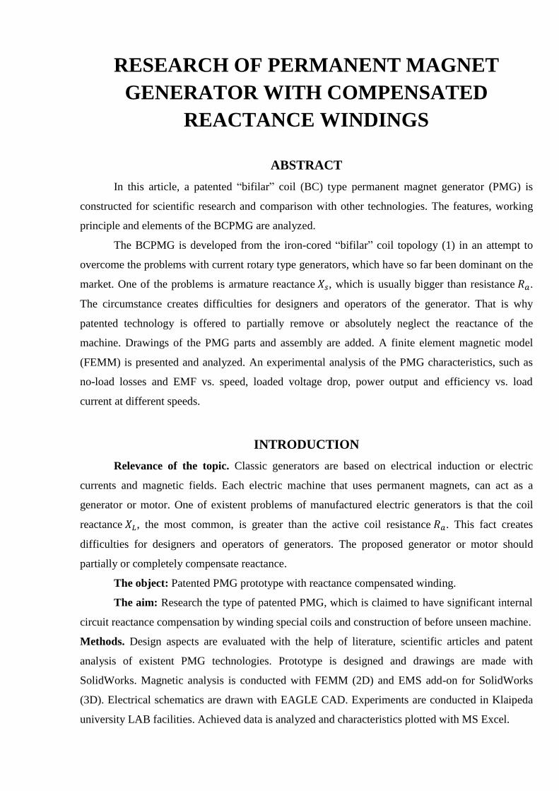
1. DESIGN ASPECTS OF PMG

1.1. Fig. 3D isometric view of PMG construction

1.1. Finite element magnetic model

A half of this PMG construction is unfolded into linear type and modeled in 2D

environment. Down below cores are shown as poles with wound coils around them and the magnets

from both sides surface mounted on iron plate. Another half of the generator is eliminated, because

it is impossible to have a full model in 2D environment.

1.2. Fig. Magnetic circuit flux lines of PMG topology with double magnets.

This topology has 4 magnets for 3 stator rods or 2 pole pairs for 3 phases. The original plan

was to put 10 permanents magnets on each of the four parts of the rotor. The reason is due to little

magnetic field interacting, if every second magnet from top and bottom is eliminated, there is only

half area left for the other magnet pole, while the first one covers a full area, which causes high

cogging torques while spinning and only half of the flux from magnets is used. This problem has

been fixed by mounting 20 permanent magnets on each of the four parts of the rotor. With the

configuration, while the one coil faces one pole (north for example), the following two coils face 3

quarters of a south pole and a quarter of a north pole so the magnetic force of the coil A is equal to

the magnetic force of the coils BC.

4

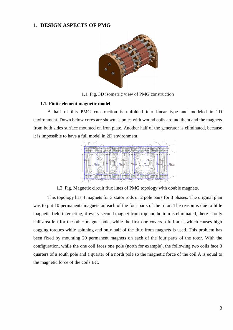
1.3. Fig. Magnetic circuit flux lines of PMG topology with fewer magnets.

A magnetic transition between rotor and stator is shown below in steps.

Step 1

Step 2

Step 3

Step 4

Step 5

Step 6

Step 7

Step n

1.4. Fig. Magnetic circuit flux lines of PMG while moving through steps.

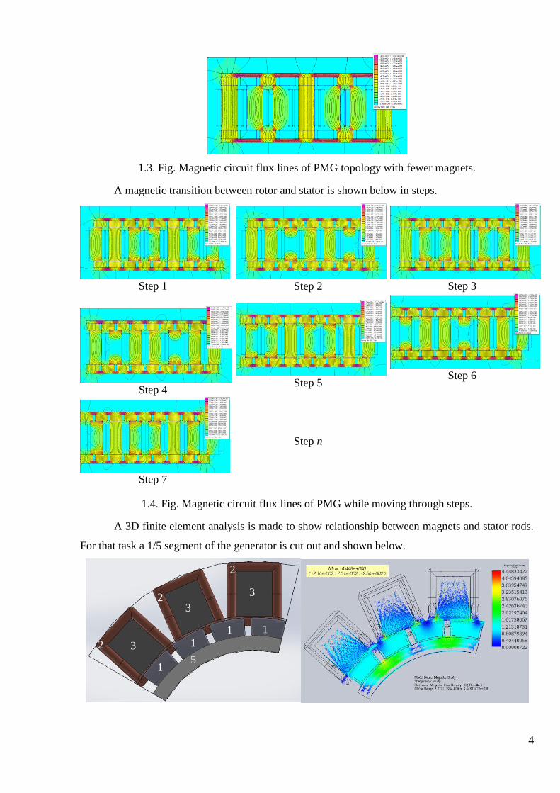
A 3D finite element analysis is made to show relationship between magnets and stator rods.

For that task a 1/5 segment of the generator is cut out and shown below.

1 5

1 1 1

3

3

3

2

2

2

5

1.5. Fig. 1/5 segment of patented PMG active material, magnetic flux density vector plot (front

view)

1) Magnets;

2) Windings;

3) Ferromagnetic cores;

4) Magnetic flux lines with direction arrow;

5) Iron or steel non-laminated core;

6) Rotor supporting part (non-magnetic);

7) Shaft.

1.6. Fig. 1/5 segment of patented PMG active material, magnetic flux density vector plot (top view)

1.7. Fig. Magnetic flux density continuous fringe plot on several sections: A – cross section of

magnet array, B – cross section of coils

1.8. Fig. Magnetic flux density continuous fringe plot on several sections: C – axial section of core

phase C, D – axial section of core phase A

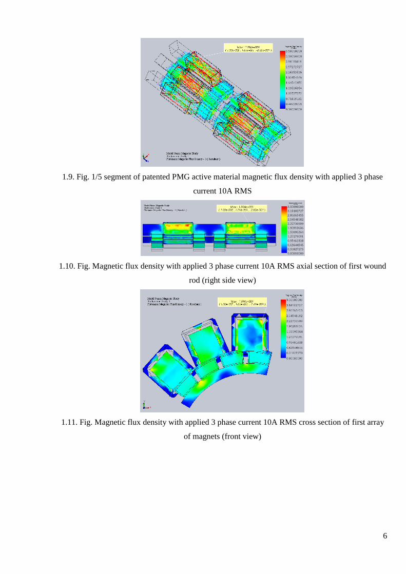
Further a 3 phase current is applied to show the relationship between wound stator and magnets.

A

B

D C

6

1.9. Fig. 1/5 segment of patented PMG active material magnetic flux density with applied 3 phase

current 10A RMS

1.10. Fig. Magnetic flux density with applied 3 phase current 10A RMS axial section of first wound

rod (right side view)

1.11. Fig. Magnetic flux density with applied 3 phase current 10A RMS cross section of first array

of magnets (front view)

7

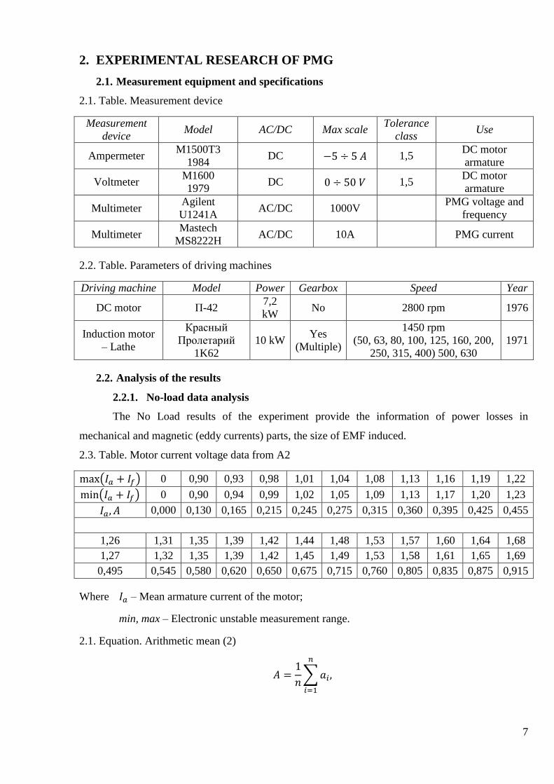
2. EXPERIMENTAL RESEARCH OF PMG

2.1. Measurement equipment and specifications

2.1. Table. Measurement device

Measurement

device Model AC/DC Max scale

Tolerance

class Use

Ampermeter M1500T3

1984 DC 1,5

DC motor

armature

Voltmeter M1600

1979 DC 1,5

DC motor

armature

Multimeter Agilent

U1241A AC/DC 1000V

PMG voltage and

frequency

Multimeter Mastech

MS8222H AC/DC 10A PMG current

2.2. Table. Parameters of driving machines

Driving machine Model Power Gearbox Speed Year

DC motor П-42 7,2

kW No 2800 rpm 1976

Induction motor

– Lathe

Красный

Пролетарий

1K62

10 kW Yes

(Multiple)

1450 rpm

(50, 63, 80, 100, 125, 160, 200,

250, 315, 400) 500, 630

1971

2.2. Analysis of the results

2.2.1. No-load data analysis

The No Load results of the experiment provide the information of power losses in

mechanical and magnetic (eddy currents) parts, the size of EMF induced.

2.3. Table. Motor current voltage data from A2

0 0,90 0,93 0,98 1,01 1,04 1,08 1,13 1,16 1,19 1,22

0 0,90 0,94 0,99 1,02 1,05 1,09 1,13 1,17 1,20 1,23

0,000 0,130 0,165 0,215 0,245 0,275 0,315 0,360 0,395 0,425 0,455

1,26 1,31 1,35 1,39 1,42 1,44 1,48 1,53 1,57 1,60 1,64 1,68

1,27 1,32 1,35 1,39 1,42 1,45 1,49 1,53 1,58 1,61 1,65 1,69

0,495 0,545 0,580 0,620 0,650 0,675 0,715 0,760 0,805 0,835 0,875 0,915

Where – Mean armature current of the motor;

min, max – Electronic unstable measurement range.

2.1. Equation. Arithmetic mean (2)

8

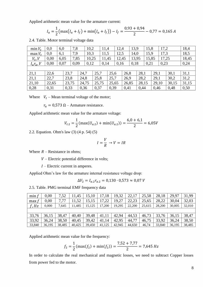
Applied arithmetic mean value for the armature current:

2.4. Table. Motor terminal voltage data

0,0 6,0 7,8 10,2 11,4 12,4 13,9 15,8 17,2 18,4

0,0 6,1 7,9 10,3 11,5 12,5 14,0 15,9 17,3 18,5

0,00 6,05 7,85 10,25 11,45 12,45 13,95 15,85 17,25 18,45

0,00 0,07 0,09 0,12 0,14 0,16 0,18 0,21 0,23 0,24

21,1 22,6 23,7 24,7 25,7 25,6 26,8 28,1 29,1 30,1 31,1

21,1 22,7 23,8 24,8 25,8 25,7 26,9 28,2 29,1 30,2 31,2

21,10 22,65 23,75 24,75 25,75 25,65 26,85 28,15 29,10 30,15 31,15

0,28 0,31 0,33 0,36 0,37 0,39 0,41 0,44 0,46 0,48 0,50

Where – Mean terminal voltage of the motor;

– Armature resistance.

Applied arithmetic mean value for the armature voltage:

2.2. Equation. Ohm's law (3) (4 p. 54) (5)

Where – Resistance in ohms;

– Electric potential difference in volts;

– Electric current in amperes.

Applied Ohm’s law for the armature internal resistance voltage drop:

2.5. Table. PMG terminal EMF frequency data

0,00 7,52 11,45 15,10 17,18 19,32 22,17 25,58 28,18 29,97 31,99

0,00 7,77 11,52 15,15 17,22 19,27 22,23 25,65 28,22 30,04 32,03

0,000 7,645 11,485 15,125 17,200 19,295 22,200 25,615 28,200 30,005 32,010

33,76 36,15 38,47 40,40 39,48 41,11 42,94 44,53 46,73 33,76 36,15 38,47

33,92 36,24 38,50 40,45 39,42 41,14 42,95 44,77 46,75 33,92 36,24 38,50 33,840 36,195 38,485 40,425 39,450 41,125 42,945 44,650 46,74 33,840 36,195 38,485

Applied arithmetic mean value for the frequency:

In order to calculate the real mechanical and magnetic losses, we need to subtract Copper losses

from power fed to the motor.

9

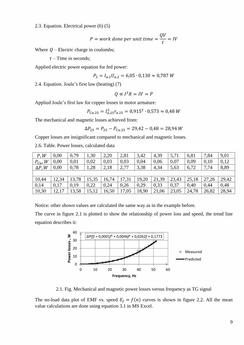
2.3. Equation. Electrical power (6) (5)

Where – Electric charge in coulombs;

– Time in seconds;

Applied electric power equation for fed power:

2.4. Equation. Joule’s first law (heating) (7)

Applied Joule’s first law for copper losses in motor armature:

The mechanical and magnetic losses achieved from:

Copper losses are insignificant compared to mechanical and magnetic losses.

2.6. Table. Power losses, calculated data

0,00 0,79 1,30 2,20 2,81 3,42 4,39 5,71 6,81 7,84 9,01

0,00 0,01 0,02 0,03 0,03 0,04 0,06 0,07 0,09 0,10 0,12

0,00 0,78 1,28 2,18 2,77 3,38 4,34 5,63 6,72 7,74 8,89

10,44 12,34 13,78 15,35 16,74 17,31 19,20 21,39 23,43 25,18 27,26 29,42

0,14 0,17 0,19 0,22 0,24 0,26 0,29 0,33 0,37 0,40 0,44 0,48

10,30 12,17 13,58 15,12 16,50 17,05 18,90 21,06 23,05 24,78 26,82 28,94

Notice: other shown values are calculated the same way as in the example before.

The curve in figure 2.1 is plotted to show the relationship of power loss and speed, the trend line

equation describes it:

2.1. Fig. Mechanical and magnetic power losses versus frequency as TG signal

The no-load data plot of EMF vs. speed curves is shown in figure 2.2. All the mean

value calculations are done using equation 3.1 in MS Excel.

ΔP(f) = 0,0001f3 + 0,0046f2 + 0,0262f + 0,1773

0

10

20

30

40

0 10 20 30 40 50 60

Po

we

r lo

sse

s , W

Frequency, Hz

Measured

Predicted

10

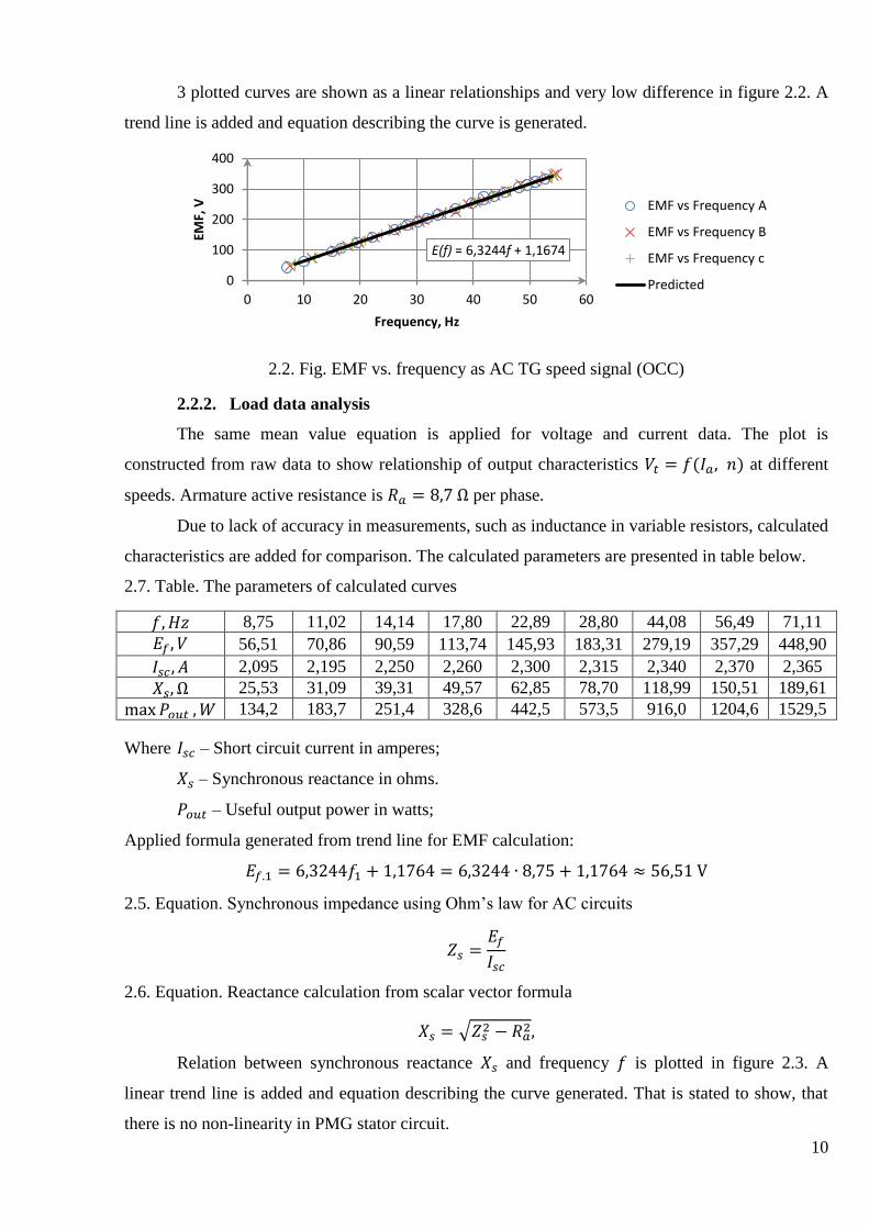
3 plotted curves are shown as a linear relationships and very low difference in figure 2.2. A

trend line is added and equation describing the curve is generated.

2.2. Fig. EMF vs. frequency as AC TG speed signal (OCC)

2.2.2. Load data analysis

The same mean value equation is applied for voltage and current data. The plot is

constructed from raw data to show relationship of output characteristics at different

speeds. Armature active resistance is per phase.

Due to lack of accuracy in measurements, such as inductance in variable resistors, calculated

characteristics are added for comparison. The calculated parameters are presented in table below.

2.7. Table. The parameters of calculated curves

8,75 11,02 14,14 17,80 22,89 28,80 44,08 56,49 71,11

56,51 70,86 90,59 113,74 145,93 183,31 279,19 357,29 448,90

2,095 2,195 2,250 2,260 2,300 2,315 2,340 2,370 2,365

25,53 31,09 39,31 49,57 62,85 78,70 118,99 150,51 189,61

134,2 183,7 251,4 328,6 442,5 573,5 916,0 1204,6 1529,5

Where – Short circuit current in amperes;

– Synchronous reactance in ohms.

– Useful output power in watts;

Applied formula generated from trend line for EMF calculation:

2.5. Equation. Synchronous impedance using Ohm’s law for AC circuits

2.6. Equation. Reactance calculation from scalar vector formula

Relation between synchronous reactance and frequency is plotted in figure 2.3. A

linear trend line is added and equation describing the curve generated. That is stated to show, that

there is no non-linearity in PMG stator circuit.

E(f) = 6,3244f + 1,1674

0

100

200

300

400

0 10 20 30 40 50 60

EMF,

V

Frequency, Hz

EMF vs Frequency A

EMF vs Frequency B

EMF vs Frequency c

Predicted

11

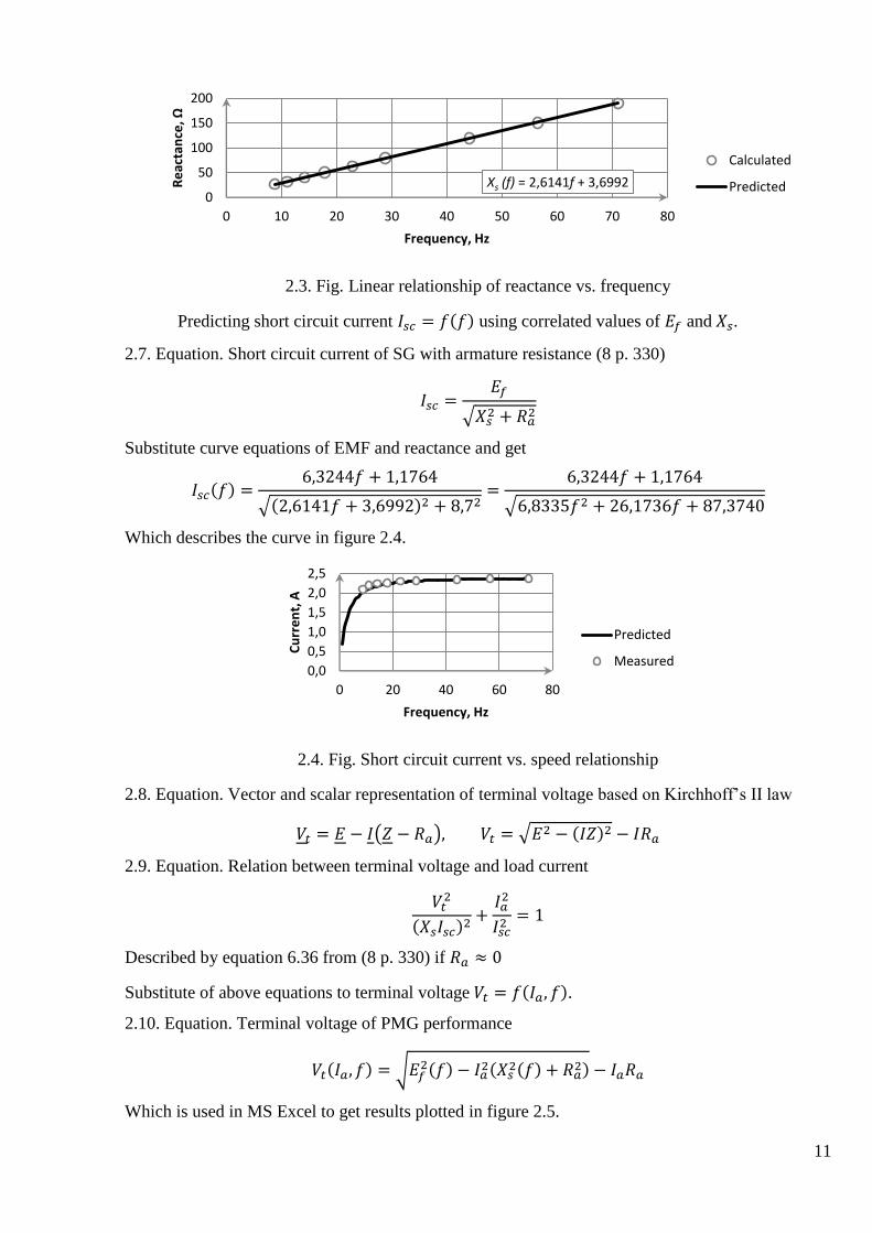
2.3. Fig. Linear relationship of reactance vs. frequency

Predicting short circuit current using correlated values of and .

2.7. Equation. Short circuit current of SG with armature resistance (8 p. 330)

Substitute curve equations of EMF and reactance and get

Which describes the curve in figure 2.4.

2.4. Fig. Short circuit current vs. speed relationship

2.8. Equation. Vector and scalar representation of terminal voltage based on Kirchhoff’s II law

2.9. Equation. Relation between terminal voltage and load current

Described by equation 6.36 from (8 p. 330) if

Substitute of above equations to terminal voltage .

2.10. Equation. Terminal voltage of PMG performance

Which is used in MS Excel to get results plotted in figure 2.5.

Xs (f) = 2,6141f + 3,6992 0

50

100

150

200

0 10 20 30 40 50 60 70 80

Re

acta

nce

, Ω

Frequency, Hz

Calculated

Predicted

0,0

0,5

1,0

1,5

2,0

2,5

0 20 40 60 80

Cu

rre

nt,

A

Frequency, Hz

Predicted

Measured

12

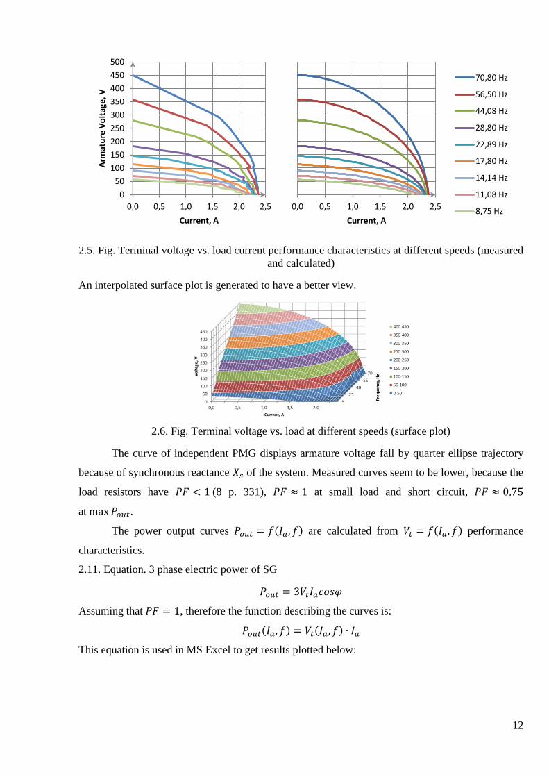
2.5. Fig. Terminal voltage vs. load current performance characteristics at different speeds (measured

and calculated)

An interpolated surface plot is generated to have a better view.

2.6. Fig. Terminal voltage vs. load at different speeds (surface plot)

The curve of independent PMG displays armature voltage fall by quarter ellipse trajectory

because of synchronous reactance of the system. Measured curves seem to be lower, because the

load resistors have (8 p. 331), at small load and short circuit,

at .

The power output curves are calculated from performance

characteristics.

2.11. Equation. 3 phase electric power of SG

Assuming that , therefore the function describing the curves is:

This equation is used in MS Excel to get results plotted below:

0

50

100

150

200

250

300

350

400

450

500

0,0 0,5 1,0 1,5 2,0 2,5

Arm

atu

re V

olt

age

, V

Current, A

0,0 0,5 1,0 1,5 2,0 2,5

Current, A

70,80 Hz

56,50 Hz

44,08 Hz

28,80 Hz

22,89 Hz

17,80 Hz

14,14 Hz

11,08 Hz

8,75 Hz

13

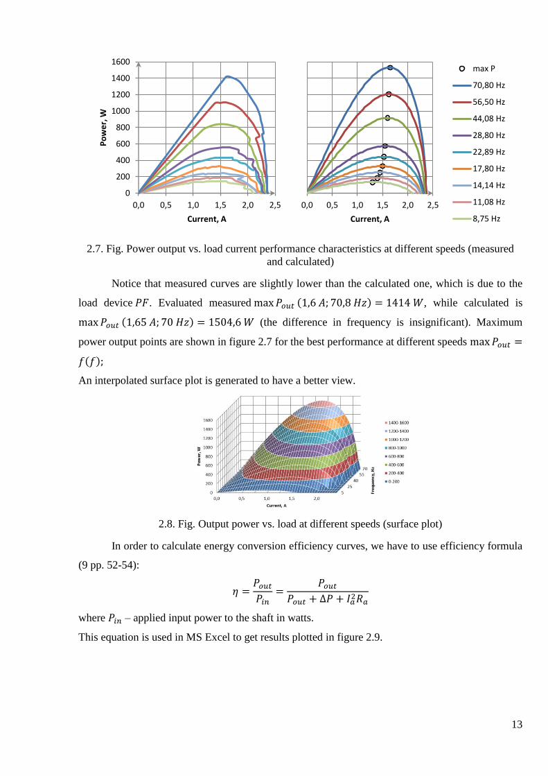
2.7. Fig. Power output vs. load current performance characteristics at different speeds (measured

and calculated)

Notice that measured curves are slightly lower than the calculated one, which is due to the

load device . Evaluated measured , while calculated is

(the difference in frequency is insignificant). Maximum

power output points are shown in figure 2.7 for the best performance at different speeds

An interpolated surface plot is generated to have a better view.

2.8. Fig. Output power vs. load at different speeds (surface plot)

In order to calculate energy conversion efficiency curves, we have to use efficiency formula

(9 pp. 52-54):

where – applied input power to the shaft in watts.

This equation is used in MS Excel to get results plotted in figure 2.9.

0

200

400

600

800

1000

1200

1400

1600

0,0 0,5 1,0 1,5 2,0 2,5

Po

we

r, W

Current, A

0,0 0,5 1,0 1,5 2,0 2,5

Current, A

max P

70,80 Hz

56,50 Hz

44,08 Hz

28,80 Hz

22,89 Hz

17,80 Hz

14,14 Hz

11,08 Hz

8,75 Hz

14

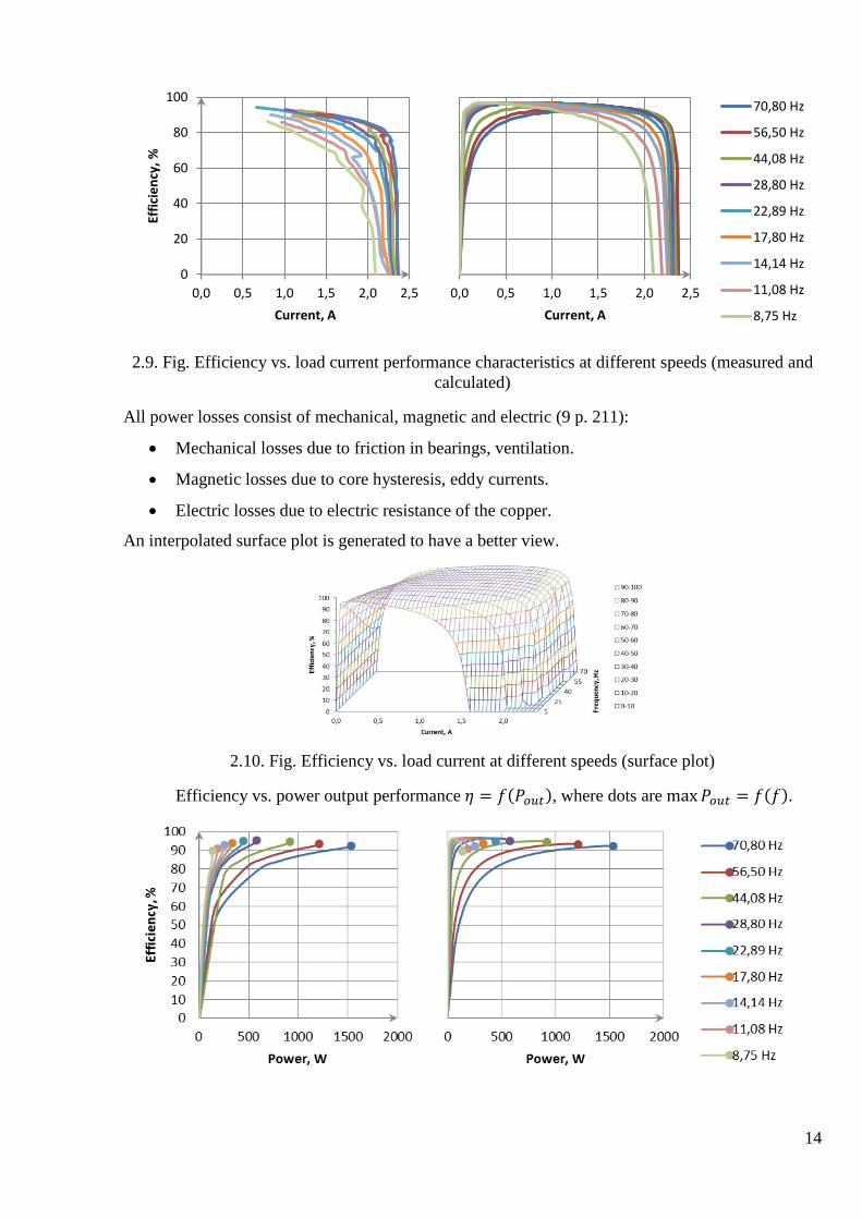
2.9. Fig. Efficiency vs. load current performance characteristics at different speeds (measured and

calculated)

All power losses consist of mechanical, magnetic and electric (9 p. 211):

Mechanical losses due to friction in bearings, ventilation.

Magnetic losses due to core hysteresis, eddy currents.

Electric losses due to electric resistance of the copper.

An interpolated surface plot is generated to have a better view.

2.10. Fig. Efficiency vs. load current at different speeds (surface plot)

Efficiency vs. power output performance , where dots are .

0

20

40

60

80

100

0,0 0,5 1,0 1,5 2,0 2,5

Effi

cie

ncy

, %

Current, A

0,0 0,5 1,0 1,5 2,0 2,5

Current, A

70,80 Hz

56,50 Hz

44,08 Hz

28,80 Hz

22,89 Hz

17,80 Hz

14,14 Hz

11,08 Hz

8,75 Hz

15

2.11. Fig. Efficiency vs. load current performance characteristics at different speeds

(before and after overload)

3. GRATITUDE

MITA (Agency of Science, Innovation and Technology) for VP2-1.3-ŪM-05-K “Inočekiai

LT” (Innovation checks) “2007-2013 growing economics program” for supporting project

“Research of innovative bifilar type electric generator or motor”.

EMWorks (ElectroMagneticWorks Inc.) for trial license of software EMS, a SolidWorks

add-on for electromagnetic analysis and simulation studies.

4. CONCLUSIONS

4.1. Parameters of the PMG and comparison

In table below parameters of patented and 2 more of reviewed generator types are shown.

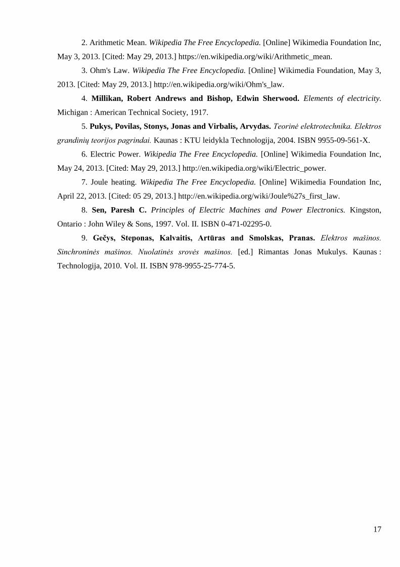
4.1. Table. Practical parameters of the PMG topology

Parameter Symbol Value

Load current 1,65

Output power 1500

Rated speed 840

No-Load EMF 446

Voltage at rated power 309

Efficiency 92,4

Rated Power factor 0,69

Total mass 55

Output power per active mass 38,4

Output power per volume 138

Number of rotors 2

Number of poles (pair poles) 20 (10)

Number of coils 30

Number of loops per coil 375

Active diameter 150

Rotor inertia 29,58

Phase armature resistance 8,7

Phase synchronous reactance 186,7

16

Phase inductance 442,5

Output frequency 70

Cooling Natural

4.2. Material consumptions

4.2. Table. Consumed material quantity

Material Mass, kg Number of pcs. or pkg.

Copper 13 30 coils

Laminated steel 20,7 15 rods 20x25x352

Non-laminated steel 4,4 4 rings, 1 shaft, fasteners

NdFeB N45 magnets 3,3 80

Wood Epoxy Fiber 10,3 5 parts

Polyethylene 1,8 2 cylindroids

Bearings 0,2 3

4.3. Experiment characteristics

Power no-load losses vs. speed characteristic is a square function of speed (frequency),

which include friction, ventilation and iron losses (induction, eddy currents), at it

reaches of power loss.

No-load EMF vs. speed (frequency) characteristic has linear relationship.

As PMG is loaded, terminal voltage fall by quarter ellipse trajectory due to synchronous

reactance . Measured curves seem to be lower due to the load resistors with

at small load and short circuit, at .

Power Output vs. load current measured curves are slightly lower than the calculated one,

which are due to the load device . Measured ,

while calculated is . For applications a max power

output points are shown in figure 2.7 for the best performance at different

speeds .

Efficiency covers a large area at different speeds and load currents, at efficiency

almost same . The bigger the speed, the bigger the load currents available

for higher efficiency, nominal thermal current is the limit, practically ,

, which is preferred to be rated, because magnet’s Curie temperature . The

machine can be driven to produce .

REFERENCE

1. Pašilis, Aleksas Alfonsas and Guseinovienė, Eleonora. Bifilar type generator or motor.

LT 2012 019 Lithaunia, March 12, 2012. Electric Machines.

17

2. Arithmetic Mean. Wikipedia The Free Encyclopedia. [Online] Wikimedia Foundation Inc,

May 3, 2013. [Cited: May 29, 2013.] https://en.wikipedia.org/wiki/Arithmetic_mean.

3. Ohm's Law. Wikipedia The Free Encyclopedia. [Online] Wikimedia Foundation, May 3,

2013. [Cited: May 29, 2013.] http://en.wikipedia.org/wiki/Ohm's_law.

4. Millikan, Robert Andrews and Bishop, Edwin Sherwood. Elements of electricity.

Michigan : American Technical Society, 1917.

5. Pukys, Povilas, Stonys, Jonas and Virbalis, Arvydas. Teorinė elektrotechnika. Elektros

grandinių teorijos pagrindai. Kaunas : KTU leidykla Technologija, 2004. ISBN 9955-09-561-X.

6. Electric Power. Wikipedia The Free Encyclopedia. [Online] Wikimedia Foundation Inc,

May 24, 2013. [Cited: May 29, 2013.] http://en.wikipedia.org/wiki/Electric_power.

7. Joule heating. Wikipedia The Free Encyclopedia. [Online] Wikimedia Foundation Inc,

April 22, 2013. [Cited: 05 29, 2013.] http://en.wikipedia.org/wiki/Joule%27s_first_law.

8. Sen, Paresh C. Principles of Electric Machines and Power Electronics. Kingston,

Ontario : John Wiley & Sons, 1997. Vol. II. ISBN 0-471-02295-0.

9. Gečys, Steponas, Kalvaitis, Artūras and Smolskas, Pranas. Elektros mašinos.

Sinchroninės mašinos. Nuolatinės srovės mašinos. [ed.] Rimantas Jonas Mukulys. Kaunas :

Technologija, 2010. Vol. II. ISBN 978-9955-25-774-5.