Research Article Supply Chain Coordination for …downloads.hindawi.com/journals/mpe/2014/649189.pdf · Research Article Supply Chain Coordination for Fixed Lifetime Products with

Research ArticleSupply Chain Coordination for Fixed Lifetime Products withPermissible Delay in Payments

Yongrui Duan, Guiping Li, and Jiazhen Huo

School of Economics and Management, Tongji University, Shanghai 200092, China

Correspondence should be addressed to Yongrui Duan; [email protected]

Received 12 February 2014; Revised 13 April 2014; Accepted 13 April 2014; Published 7 May 2014

Academic Editor: Ming Li

Copyright © 2014 Yongrui Duan et al. This is an open access article distributed under the Creative Commons Attribution License,which permits unrestricted use, distribution, and reproduction in any medium, provided the original work is properly cited.

This paper considers a two-level supply chain coordination problem for fixed lifetime products with permissible delay in payments.Two cases are discussed; that is, the retailer is required to settle the balance before the end of the ordering cycle (Case I) and afterthe ordering cycle (Case II).The coordination models are proposed and analyzed, respectively.The analytical methods as to how todetermine the optimal policy are presented. In addition, it is indicated that the supplier’s cost as well as that of the total system willbe reduced no matter how much the parameters change, and the retailer will benefit from coordination, if the supplier is willingto share the cost saving with him/her in Case I. In Case II, the retailer’s average cost will be reduced and the supplier will benefitfrom coordination only under certain conditions. Besides, the results show that, for fixed lifetime products, providing longer creditperiod than the retailer’s order period is not commonly applicable.

1. Introduction

In recent years, the area of supply chain management hasbecome very popular.Many researchers have devoted consid-erable attention to coordination issues between suppliers andretailers in a supply chain. A variety of coordination mecha-nisms are developed and utilized in the different settings.

Monahan [1] studied a single supplier-single buyer distri-bution system and indicated that the supplier could improvechannel coordination and earn higher profits by offeringthe buyer a quantity discount. Later, Lee and Rosenblatt[2] generalized Monahan’s model by relaxing his lot-for-lotassumption for the supplier. Shin and Benton [3] studied theeffectiveness of quantity discounts under different conditions.They showed that the link between quantity discounts andthe performance of the chain is influenced by several otherfactors including the variability of demand, the relativeinventory cost structures, and the buyer’s economic reorderintervals. Jaber and Osman [4] proposed a centralized modelwhere the players in a two-level supply chain coordinatedtheir orders through delay in payments to minimize theirlocal costs and that of the chain. Chen andKang [5] developedthe integrated models with permissible delay in payment fordetermining the coefficient of negotiation and the maximum

delay payment period. Sarmah et al. [6] studied a coordina-tion mechanism through credit option such that both partiescan divide the surplus equitably after satisfying their ownprofit targets. Emmons and Gilbert [7] studied the effect ofreturn policies on both manufacturer and retailer’s profits.In their model, demand is uncertain and price-dependent.Giannoccaro and Pontrandolfo [8] coordinated a three-stagesupply chain with a stochastic customer demand by using therevenue sharing policy. Extensive reviews of the literature onsupply chain coordination are available in [9, 10].

In the supply chain coordination literatures that havebeen mentioned above, the researchers all ignored the con-straint of items’ finite lifetime in their models. In fact, manyproducts or goods have their own sell-by dates. Foodstuff,such as bread, milk, and beverage, all become unusable aftera certain time. Photographic material, blood, and drugs arefurther examples of items with fixed lifetime. Moreover, theupgrade of IT products, the launch of new products, and thechange of popularity make more and more products havea certain lifetime. In the past few decades, the inventoryoptimization of the finite lifetime product has been the focusofmany researchers. Nahmias [11] classified the finite lifetimeproblem into two subcategories: random finite lifetime andfixed finite lifetime.The randomfinite lifetime products, such

Hindawi Publishing CorporationMathematical Problems in EngineeringVolume 2014, Article ID 649189, 11 pageshttp://dx.doi.org/10.1155/2014/649189

2 Mathematical Problems in Engineering

as fruit and vegetable, spoil over time and the value alsodecreases gradually. Itemswith the fixed finite lifetime, on theother hand, perish at the same age; that is, the value remainsthe same during the lifetime period and equals to zero afterthe expiration date. The relevant researches such as [12–17]are about the random finite lifetime products. Goyal and Giri[18] provided an excellent and detailed review of research oninventory problem of this kind of product. The researchesabout the fixed finite lifetime products can refer to [19–26]and their related references.

However, the above researches on fixed finite lifetimeproduct are on single stage problem. Duan et al. [27]considered a single-vendor, single-buyer supply chain forfixed lifetime product and proposed models to analyze thebenefit of coordinating supply chain through a quantitydiscount strategy. In addition, they proved that the quantitydiscount strategy can achieve system optimization and win-win outcome.

Delay in payment is one of the commonly used mecha-nisms in supply chain coordination practice. In real world,the supplier often utilizes this policy to promote his/herproducts, especially when the retailer is short of capital. Inthis policy, the supplier requires the retailer to increase hisorder size by offering the retailer a delay period. And theretailer is required to settle the balance before the end ofthe delay period. During the delay period, the retailer cancumulate revenues and earn interests. The policy can reducethe retailer’s capital cost tied up in stock, because it reducesthe amount of capital invested in stock for the duration ofthe delay period, so that the retailer’s holding cost of financeis reduced. The policy can also decrease supplier’s orderingcost, but it adds an additional dimension of default risk to thesupplier.

Duan et al. [28] dealt with a supply chain coordinationproblem through delay in payments for items with fixedlifetime, where the costs of the supplier and retailer includethe ordering cost and the storage cost. The opportunity costof capital cost is not considered. However, when the productsare kept in the warehouse, a large amount of capital willbe backlogged, which will incur great opportunity cost inaddition to the storage cost. Furthermore, in this paper, weconsider supply chain coordination issues for fixed lifetimeproduct through delay in payment. In the delay in paymentcontract, the supplier will provide a credit period for theretailer. In this case, the capital cost of the retailer is anonlinear and a piecewise function of time. So it is necessaryto investigate how the optimal policy is changed when capitalcost is considered. The main differences between Duan etal. [28] and this paper are as follows. Firstly, in additionto the ordering and storage cost, this paper considers theopportunity cost of capital in the model formulation, whichis not considered in [28]; secondly, because the retailer’sopportunity costs of capital backlogging are dependent onthe time when the balance are settled, we discuss two cases.Case I: the retailer is required to settle the balance beforethe end of the ordering cycle and Case II: the retailer settlesthe balance after the ordering cycle. Thirdly, we find thatwhen the opportunity cost is not considered, the supplier willalways benefit no matter how much the parameters change,

and the cost of the retailer will not change. However, whenthe opportunity cost is considered and the retailer settles thebalance after the ordering cycle, then the cost of the suppliermay increase but the cost of the retailer may decrease. So theopportunity costs have significant influence on the optimalcoordination policy.

The rest of this paper is organized as follows. In Section 2,the supply chain coordination model to minimize the sup-plier’s cost is formulated, and the analytically tractablesolutions are derived. A numerical study is conducted inSection 3 to illustrate the performance of the proposed policyand examine the implications of the change in the value ofparameters. The concluding remarks are presented in the lastsection.

2. Model Formulation

In this section, we formulate and analyze the decision-making models of a two-level supply chain for fixed lifetimeproducts without and with coordination. In the absence ofcoordination, both of the parties make decisions to minimizetheir own costs. In the presence of coordination, the supplieris the decision-maker of the supply chain with the objectiveof minimizing his/her own cost, and the delay in paymentsis adopted as a coordination policy. In addition, we obtainthe optimal policies for the different cases and find that thelifetime of the product is an important constraint in theoptimal policies.

We adopt the same assumptions as in Duan et al.[28] which are also commonly used in the literatures, seeMonahan [1] and Lee and Rosenblatt [2].

(i) Demand is exogenous and constant.Themain reasonof this assumption is to simplify the model formu-lation and to derive the closed-form solution to themodel.

(ii) Replenishment is instantaneous and lead time is zero.Obviously, if the lead time is constant and not zero,the supplier and retailer just need to place an order aperiod exactly equal to the lead time in advance [2],and the same results can be obtained.

(iii) Shortages are not allowed. For fixed lifetime products,due to their limited lifetime, the customers wouldpurchase only when they are to be used up. If stock-out happens, most of them will buy the substituteproducts. In addition, because the demand is assumedto be constant in this paper, the shortage can beeliminated by increasing the ordering quantity.

(iv) All items ordered by the supplier arrive new and fresh;that is, their age equals zero [29]. In fact, if the items’age is 𝑙 when they arrive, we only need to replacethe product lifetime 𝐿 by 𝐿 = 𝐿 − 𝑙 in the followinganalysis.

Notations used in this paper are as follows:

𝑖 denotes the subscript identifying a specific level ina supply chain (𝑖 = 𝑠, 𝑟, where 𝑠 = supplier and 𝑟 =

retailer);

Mathematical Problems in Engineering 3

𝐷 denotes the constant demand rate;𝐴𝑖is the ordering cost of level 𝑖;

ℎ𝑖is the holding cost of finance per unit per unit time,

representing the cost of capital at level 𝑖 excluding thestorage cost;𝑠𝑖is the storage cost per unit per unit time at level 𝑖

excluding the holding cost;𝑐𝑖is the procurement cost per unit for level 𝑖;

𝑘𝑖is the return on investment for level 𝑖;

𝑄0is the retailer’s EOQ, and 𝑡

0is the order period of

the retailer in the absence of any coordination;𝐿 denotes the lifetime of product and 𝐿 ≥ 𝑡

0;

𝑇𝐶𝑠and 𝑇𝐶

𝑟are the average costs of the supplier and

the retailer in the absence of coordination;𝑇𝐶𝑠and 𝑇𝐶

𝑟are the average costs of the supplier and

the retailer in the presence of coordination.

Decision Variables

𝜇 denotes the supplier’s order multiple in the absenceof any coordination;𝐾 denotes the retailer’s order multiple in the presenceof coordination and 𝐾𝑄

0is the retailer’s new order

size;𝑡(𝐾) denotes the credit period offered to the retailer,if he orders 𝐾𝑄

0every interval of 𝐾𝑡

0(interest free

period);𝜆 denotes the supplier’s ordermultiple in the presenceof coordination.

2.1. Model Formulation for System without Coordination. Inthis subsection, the decision-making model for fixed lifetimeproducts without coordination is formulated.The retailer andthe supplier make decisions by minimizing their own costs.

In the absence of any coordination, the retailer’s orderquantity is simply the EOQ; that is,

𝑄0= √

2𝐷𝐴𝑟

ℎ𝑟+ 𝑠𝑟

. (1)

Let 𝑇𝐶𝑟denote the retailer’s average cost per unit time

and let 𝑡0denote the retailer’s optimal order period; then

𝑇𝐶𝑟= √2𝐷𝐴

𝑟(ℎ𝑟+ 𝑠𝑟),

𝑡0= √

2𝐴𝑟

𝐷(ℎ𝑟+ 𝑠𝑟).

(2)

Since the retailer’s order quantity is fixed at 𝑄0, the

supplier is faced with a stream of demands, each with ordersize 𝑄

0and at fixed intervals of 𝑡

0. Given such a stream of

demands, the supplier’s economic order quantity should besome integer multiple of𝑄

0[2]. Let 𝜇𝑄

0denote the supplier’s

order quantity where 𝜇 is a positive integer.

The supplier’s average inventory held up per unit time is

[(𝜇 − 1)𝑄0+ (𝜇 − 2)𝑄

0+ ⋅ ⋅ ⋅ + 𝑄

0+ 0𝑄0]

𝜇=

(𝜇 − 1)𝑄0

2.

(3)

The supplier’s cost per unit time is

𝑇𝐶𝑠(𝜇) =

𝐷𝐴𝑠

𝜇𝑄0

+ (ℎ𝑠+ 𝑠𝑠)(𝜇 − 1)𝑄

0

2. (4)

Hence, the supplier’s problem in the absence of coordina-tion can be formulated as follows:

min 𝑇𝐶𝑠(𝜇) =

𝐷𝐴𝑠

𝜇𝑄0

+ (ℎ𝑠+ 𝑠𝑠)(𝜇 − 1)𝑄

0

2

s.t.𝜇𝑄0

𝐷≤ 𝐿, 𝜇 ≥ 1 is an integer.

(5)

By substituting 𝑄0into (5), we get

min 𝑇𝐶𝑠(𝜇) =

𝐴𝑠

𝜇√

𝐷 (ℎ𝑟+ 𝑠𝑟)

2𝐴𝑟

+ (ℎ𝑠+ 𝑠𝑠) (𝜇 − 1)√

𝐷𝐴𝑟

2 (ℎ𝑟+ 𝑠𝑟)

s.t. 𝜇√2𝐴𝑟

𝐷(ℎ𝑟+ 𝑠𝑟)≤ 𝐿, 𝜇 ≥ 1 is an integer.

(6)

Thefirst constraint in (6) is to ensure that the products arenot overdue before they are sold out. In this case, the supplierwill minimize his average cost by selecting the optimal ordermultiple 𝜇. In the next section, we will give the analyticalsolution to (6).

Lemma 1. If 𝐿 ≥ 𝑡0

= √2𝐴𝑟/𝐷(ℎ𝑟+ 𝑠𝑟), then the supplier’s

optimal order multiple is as follows:

𝜇∗= min {𝜇

∗

1, 𝜇∗

2} , (7)

where 𝜇∗

1= ⌈√1/4 + 𝐴

𝑠(ℎ𝑟+ 𝑠𝑟)/𝐴𝑟(ℎ𝑠+ 𝑠𝑠) − 1/2⌉, 𝜇∗

2=

[𝐿√𝐷(ℎ𝑟+ 𝑠𝑟)/2𝐴𝑟], ⌈𝑥⌉ denotes the least integer greater than

or equal to 𝑥; [𝑥] denotes the integer part of 𝑥.

The proof of Lemma 1 can refer to Duan et al. [28].Lemma 1 gives the supplier’s optimal order multiple of theretailer’s ordering quantity without coordination. Here, 𝐿 ≥

𝑡0is to ensure that the EOQmodel is to ensure that the items

are not expired before they are sold out.

2.2. Model Formulation for System with Coordination. In thissubsection, we will propose and discuss the supply chaincoordinationmodel for fixed lifetime products through delayin payments policy. In this policy, the retailer orders 𝐾𝑄

0

units products every interval of 𝐾𝑡0from the supplier at a

unit purchasing cost 𝑐𝑟and the ordering cost𝐴

𝑟.The supplier

orders 𝜆𝐾𝑄0units every interval of 𝜆𝐾𝑡

0and offers the credit


period 𝑡(𝐾) to the retailer, where 𝐾, 𝜆, and 𝑡(𝐾) are decisionvariables. Meanwhile, the retailer has the opportunity toinvest the unpaid balance 𝑐

𝑟𝐾𝑄0for a period 𝑡(𝐾) at a return

rate of 𝑘𝑟. That is, if the retailer can settle his balance at the

time 𝑡(𝐾), they will have a capital gain of 𝑐𝑟𝐾𝑄0𝑘𝑟𝑡(𝐾), but

the supplier’s cost will be increased by 𝑐𝑟𝐾𝑄0𝑘𝑠𝑡(𝐾).

Therefore, the supplier’s cost per unit time 𝑇𝐶𝑠(𝐾, 𝜆) is

composed of the following:

(i) the supplier’s ordering cost per unit time which isequal to 𝐷𝐴

𝑠/𝜆𝐾𝑄

0,

(ii) the supplier’s holding cost of finance per unit timewhich is equal to ℎ

𝑠𝐾𝑄0(𝜆 − 1)/2 + ℎ

𝑠𝐷𝑡(𝐾),

(iii) the supplier’s storage cost per unit time which is equalto 𝑠𝑠𝐾𝑄0(𝜆 − 1)/2,

(iv) the supplier’s opportunity cost per unit time which isequal to 𝑐

𝑟𝐷𝑘𝑠𝑡(𝐾).

Hence,

𝑇𝐶𝑠 (𝐾, 𝜆) =

𝐷𝐴𝑠

𝜆𝐾𝑄0

+(ℎ𝑠+ 𝑠𝑠)𝐾𝑄0 (𝜆 − 1)

2

+ ℎ𝑠𝐷𝑡 (𝐾)+𝑐

𝑟𝐷𝑘𝑠𝑡 (𝐾) .

(8)

The retailer’s cost consists of the following:

(i) the retailer’s ordering cost per cycle which is equal to𝐴𝑟,

(ii) the retailer’s holding cost of finance per cycle which isequal to

𝐻𝑟 (𝐾) =

{{

{{

{

ℎ𝑟

(𝐾𝑄0− 𝐷𝑡 (𝐾))

2

2𝐷, 0 ≤ 𝑡 (𝐾) ≤ 𝐾𝑡

0

0, 𝑡 (𝐾) ≥ 𝐾𝑡0,

(9)

(iii) the retailer’s storage cost per cycle which is equal to𝑠𝑟𝐾2𝑄0𝑡0/2,

(iv) the retailer’s revenue during the credit period whichis equal to 𝑐

𝑟𝐾𝑄0𝑘𝑟𝑡(𝐾).

Therefore, the retailer’s cost per unit time is

𝑇𝐶𝑟 (𝐾) =

𝐴𝑟+ 𝐻𝑟 (𝐾) + 𝑠

𝑟𝐾2𝑄0𝑡0/2 − 𝑐

𝑟𝐾𝑄0𝑘𝑟𝑡 (𝐾)

𝐾𝑡0

=𝐷𝐴𝑟

𝐾𝑄0

+𝐷𝐻𝑟 (𝐾)

𝐾𝑄0

+𝑠𝑟𝐾𝑄0

2− 𝑐𝑟𝐷𝑘𝑟𝑡 (𝐾) .

(10)

To entice the retailer to accept this policy, the suppliershould ensure that the retailer’s average cost per unit timewith coordination is not greater than that without anycoordination. The coordination problem can be formulatedas the following mathematical programming:

min 𝑇𝐶𝑠 (𝐾, 𝜆)

s.t. 𝜆𝐾𝑡0≤ 𝐿

𝑇𝐶𝑟 (𝐾) ≤ 𝑇𝐶

𝑟

𝜆 ≥ 1 is an integer.

(11)

The first constraint of (11) is to guarantee that thesupplier’s products are not overdue before they are sold out.The second constraint is to ensure that the policy proposedby the supplier is acceptable to the retailer.

Based on the value of 𝐻𝑟(𝐾), two cases are discussed,

respectively, in the following, namely, Case I: 0 ≤ 𝑡(𝐾) ≤ 𝐾𝑡0

and Case II: 𝑡 ≥ 𝐾𝑡0.

Case I. When 0 ≤ 𝑡(𝐾) ≤ 𝐾𝑡0, 𝐻𝑟(𝐾) = ℎ

𝑟(𝐾𝑄0− 𝐷𝑡(𝐾))

2/

2𝐷.In this case, (11) is reduced to the following problem:

min 𝑇𝐶𝑠 (𝐾, 𝜆) =

𝐷𝐴𝑠

𝜆𝐾𝑄0

+(ℎ𝑠+ 𝑠𝑠)𝐾𝑄0 (𝜆 − 1)

2

+ ℎ𝑠𝐷𝑡 (𝐾) + 𝑐

𝑟𝐷𝑘𝑠𝑡 (𝐾)

s.t. 𝜆𝐾𝑄0

𝐷≤ 𝐿

𝐷𝐴𝑟

𝐾𝑄0

+ℎ𝑟(𝐾𝑄0− 𝐷𝑡 (𝐾))

2

2𝐾𝑄0

+𝑠𝑟𝐾𝑄0

2

− 𝑐𝑟𝐷𝑘𝑟𝑡 (𝐾) ≤ √2𝐷𝐴

𝑟(ℎ𝑟+ 𝑠𝑟)

𝜆 ≥ 1.

(12)

Theorem 2. Let 𝜇∗ and 𝜆

∗ be the supplier’s optimal ordermultiple without and with coordination, and let 𝐾

∗ be theretailer’s optimal order multiple with coordination; then

𝑇𝐶𝑠(𝐾∗, 𝜆∗) ≤ 𝑇𝐶

𝑠(𝜇∗) . (13)

Proof. It is easy to verify that 𝑇𝐶𝑠(𝐾, 𝜆) is increasing in 𝑡(𝐾).

𝑇𝐶𝑟(𝐾) is convex and decreasing in 𝑡(𝐾), for 0 ≤ 𝑡(𝐾) ≤ 𝐾𝑡

0.

As a result, the objective function of (12) is minimized whenthe second constraint is an equation; that is,

𝐷𝐴𝑟

𝐾𝑄0

+𝐷ℎ𝑟

𝐾𝑄0

(𝐾𝑄0− 𝐷𝑡 (𝐾))

2

2𝐷+

𝑠𝑟𝐾𝑄0

2

− 𝑐𝑟𝐷𝑘𝑟𝑡 (𝐾) = √2𝐷𝐴

𝑟(ℎ𝑟+ 𝑠𝑟).

(14)

By rearranging the terms, we have

ℎ𝑟

2(𝐷𝑡 (𝐾))

2− (ℎ𝑟+ 𝑐𝑟𝑘𝑟)𝐾𝑄0𝐷𝑡 (𝐾) + 𝐴

𝑟𝐷(𝐾 − 1)

2= 0.

(15)

Let 𝑡1≤ 𝑡2be the two roots of (15); then, if (ℎ

𝑟+𝑐𝑟𝑘𝑟)2𝑄2

0𝐾2−

2ℎ𝑟𝐴𝑟𝐷(𝐾 − 1)

2≥ 0,

𝑡1=

(ℎ𝑟+ 𝑐𝑟𝑘𝑟)𝐾𝑄0− √(ℎ

𝑟+ 𝑐𝑟𝑘𝑟)2𝐾2𝑄20− 2ℎ𝑟𝐴𝑟𝐷(𝐾− 1)

2

ℎ𝑟𝐷

,

𝑡2=

(ℎ𝑟+ 𝑐𝑟𝑘𝑟)𝐾𝑄0+ √(ℎ

𝑟+ 𝑐𝑟𝑘𝑟)2𝐾2𝑄20− 2ℎ𝑟𝐴𝑟𝐷(𝐾− 1)

2

ℎ𝑟𝐷

.

(16)


Since (ℎ𝑟+𝑐𝑟𝑘𝑟)𝐾𝑄0> 0 and𝐴

𝑟𝐷(𝐾−1)

2> 0, for𝐾 > 1, then

𝑡1> 0 and 𝑡

2> 0. In addition, by noting that 𝑡∗(𝐾) ≤ 𝐾𝑄

0/𝐷,

we have

𝑡∗(𝐾)

=(ℎ𝑟+ 𝑐𝑟𝑘𝑟)𝐾𝑄0− √(ℎ

𝑟+ 𝑐𝑟𝑘𝑟)2𝐾2𝑄20− 2ℎ𝑟𝐴𝑟𝐷(𝐾 − 1)

2

ℎ𝑟𝐷

.

(17)

It can be seen from (17) that, if 𝐾 = 1, then 𝑡∗(𝐾) = 0. (12) is

reduced to (6), if𝐾 = 1, so (13) holds.The proof ofTheorem 2is complete.

Theorem 2 indicates that the supplier’s cost as well asthat of the system can be reduced in the proposed delayin payment policy, and the retailer’s cost is not changed. Inpractice, the supplier will usually share the saving cost withthe retailer, and the sharing rate is determined by their powerof balance between them.

Theorem 3. The retailer’s order size with coordination isgreater than that without coordination; that is, 𝐾 ≥ 1.

Proof. Since

𝑑2𝑡∗(𝐾)

𝑑𝐾2= 2[(ℎ

𝑟+ 𝑐𝑟𝑘𝑟)2𝐾2𝑄2

0− 2ℎ𝑟𝐴𝑟𝐷(𝐾 − 1)

2]−3/2

× (ℎ𝑟+ 𝑐𝑟𝑘𝑟)2ℎ𝑟𝐴𝑟𝐷𝑄2

0> 0,

(18)

𝑡∗(𝐾) is convex in 𝐾. In addition, it is easy to verify that

𝑑𝑡∗(𝐾)/𝑑𝐾|

𝐾=1= 0; so 𝑡

∗(𝐾) is minimized, when 𝐾 = 1.

In practice, the more the retailer orders, the longer the delayperiod should be; so 𝑡

∗(𝐾) should increase in𝐾. It is straight

forward that only if 𝐾 ≥ 1, 𝑡∗(𝐾) is increasing in 𝐾. As aresult, 𝐾 ≥ 1 holds. The proof of Theorem 3 is complete.

Theorem 3 demonstrates that delay in payments policycan indeed induce the retailer to increase his/her orderquantity.

Then, we will prove 𝑡∗(𝐾) ≤ 𝐾𝑡

0.

Proposition 4. If 𝑠𝑟> 2𝑐𝑟𝑘𝑟, then 0 ≤ 𝑡

∗(𝐾) ≤ 𝐾𝑡

0holds for

1 ≤ 𝐾 ≤ 𝐾1, where 𝐾

1= 1/(1 − √(ℎ

𝑟+ 2𝑐𝑟𝑘𝑟)/(ℎ𝑟+ 𝑠𝑟)).

Proof. The condition for the existence of 𝑡∗(𝐾) is

(ℎ𝑟+ 𝑐𝑟𝑘𝑟)2𝑄2

0𝐾2− 2ℎ𝑟𝐴𝑟𝐷(𝐾 − 1)

2≥ 0; (19)

that is

(ℎ𝑟+ 𝑐𝑟𝑘𝑟)2

ℎ𝑟(ℎ𝑟+ 𝑠𝑟)

≥(𝐾 − 1)

2

𝐾2. (20)

In addition, to prove that 𝑡∗(𝐾) ≤ 𝐾𝑄0/𝐷 holds, that is,

(ℎ𝑟+ 𝑐𝑟𝑘𝑟)𝐾𝑄0− √(ℎ

𝑟+ 𝑐𝑟𝑘𝑟)2𝐾2𝑄20− 2ℎ𝑟𝐴𝑟𝐷(𝐾 − 1)

2

ℎ𝑟𝐷

≤𝐾𝑄0

𝐷,

(21)

we only need to prove that the following inequality holds:

ℎ𝑟+ 2𝑐𝑟𝑘𝑟

ℎ𝑟+ 𝑠𝑟

≥(𝐾 − 1)

2

𝐾2. (22)

By (ℎ𝑟+ 𝑐𝑟𝑘𝑟)2/ℎ𝑟(ℎ𝑟+ 𝑠𝑟) ≥ (ℎ

𝑟+ 2𝑐𝑟𝑘𝑟)/(ℎ𝑟+ 𝑠𝑟), we

know whether (ℎ𝑟+ 2𝑐𝑟𝑘𝑟)/(ℎ𝑟+ 𝑠𝑟) ≥ (𝐾 − 1)

2/𝐾2; then

(ℎ𝑟+ 𝑐𝑟𝑘𝑟)2/ℎ𝑟(ℎ𝑟+ 𝑠𝑟) ≥ (𝐾 − 1)

2/𝐾2 holds. Therefore,

1 ≤ 𝐾 ≤1

1 − √(ℎ𝑟+ 2𝑐𝑟𝑘𝑟) / (ℎ𝑟+ 𝑠𝑟)

. (23)

Set 𝐾1= 1/(1 − √(ℎ

𝑟+ 2𝑐𝑟𝑘𝑟)/(ℎ𝑟+ 𝑠𝑟)). By 𝐾 ≥ 1, we have

𝐾1≥ 1; that is, 𝑠

𝑟> 2𝑐𝑟𝑘𝑟. If 𝑠𝑟> 2𝑐𝑟𝑘𝑟and (23) holds, it is

easy to verify that 𝑡∗(𝐾) exists and 𝑡∗(𝐾) ≤ 𝐾𝑡

0. The proof of

Proposition 4 is complete.

Proposition 4 shows that when the retailer’s storage costis large, to reduce the storage cost, the retailer will not ordertoo much items in the beginning of every ordering cycle.Accordingly, the trade credit period offered by the supplierwill be less than the ordering cycle of the retailer.

Next, we will determine the supplier and the retailer’soptimal ordering quantities𝐾∗ and 𝜆

∗.By substituting (17) into (12), we have


𝐴𝑠𝐷

𝜆𝐾𝑄0

+ [(ℎ𝑠+ 𝑠𝑠) (𝜆 − 1)

2

+(𝑐𝑟𝑘𝑠+ℎ𝑠) (ℎ𝑟+𝑐𝑟𝑘𝑟)

ℎ𝑟

]𝐾𝑄0

−(𝑐𝑟𝑘𝑠+ℎ𝑠)

ℎ𝑟

×((ℎ𝑟+𝑐𝑟𝑘𝑟)2𝐾2𝑄2

0

−2ℎ𝑟𝐴𝑟𝐷(𝐾 − 1)

2)1/2

s.t. 𝜆𝐾𝑄0

𝐷≤ 𝐿, 𝜆 ≥ 1.

(24)

Since

𝜕2𝑇𝐶𝑠 (𝐾, 𝜆)

𝜕𝐾2

=2𝐴𝑠𝐷

𝜆𝑄0𝐾3

+2 (𝑐𝑟𝑘𝑠+ ℎ𝑠) (ℎ𝑟+ 𝑐𝑟𝑘𝑟)2𝐴𝑟𝐷𝑄2

0

× [(ℎ𝑟+𝑐𝑟𝑘𝑟)2𝑄2

0𝐾2− 2ℎ𝑟𝐴𝑟𝐷(𝐾 − 1)

2]−3/2

> 0,

(25)


then 𝑇𝐶𝑠(𝐾, 𝜆) is convex in 𝐾, for 1 ≤ 𝐾 ≤ 𝐾

1. Let 𝐾∗

1and

𝜆∗

1be the solutions ofmin𝑇𝐶

𝑠(𝐾, 𝜆), then, for given 𝜆,𝐾∗

1(𝜆)

satisfies 𝜕𝑇𝐶𝑠(𝐾, 𝜆)/𝜕𝐾 = 0.

Since 𝜆 is an integer and 𝜆 ≤ 𝐿/𝑡0, we can get 𝐾∗

1and 𝜆

∗

1

by the enumeration method.Therefore, we have the following results:

(a) if 1 ≤ 𝐾∗

1< 𝐾1, then 𝐾

∗= 𝐾∗

1and 𝜆

∗= 𝜆∗

1;

(b) if 𝐾∗1≥ 𝐾1, then 𝐾

∗= 𝐾1.

If 𝐾∗1

≥ 𝐾1, then 𝐾

∗= 𝐾1. By substituting 𝐾

∗= 𝐾1into

(24), we get

min 𝑇𝐶𝑠 (𝜆)

=𝐴𝑠𝐷

𝜆𝑄0

(1 − √ℎ𝑟+ 2𝑐𝑟𝑘𝑟

ℎ𝑟+ 𝑠𝑟

)

+ [ℎ𝑠+ 𝑠𝑠

2(𝜆 − 1) +

[𝑐𝑟𝑘𝑠+ ℎ𝑠] (ℎ𝑟+ 𝑐𝑟𝑘𝑟)

ℎ𝑟

]

×𝑄0

1 − √(ℎ𝑟+ 2𝑐𝑟𝑘𝑟) / (ℎ𝑟+ 𝑠𝑟)

−𝑐𝑟𝑘𝑠+ℎ𝑠

ℎ𝑟

([[

[

(ℎ𝑟+𝑐𝑟𝑘𝑟) 𝑄0

1−√(ℎ𝑟+2𝑐𝑟𝑘𝑟) / (ℎ𝑟+𝑠𝑟)

]]

]

2

−2ℎ𝑟𝐴𝑟𝐷(ℎ𝑟+2𝑐𝑟𝑘𝑟)

(√ℎ𝑟+𝑠𝑟−√ℎ𝑟+2𝑐𝑟𝑘𝑟)2)

1/2

s.t. 𝜆

1 − √(ℎ𝑟+ 2𝑐𝑟𝑘𝑟) / (ℎ𝑟+ 𝑠𝑟)

𝑄0

𝐷≤ 𝐿, 𝜆 ≥ 1.

(26)

It is easy to verify that 𝑇𝐶𝑠(𝜆) is convex in 𝜆. Simi-

lar to the Proof of Lemma 1, we can get that if 𝐿 ≥

√2𝐴𝑟/√𝐷(√ℎ

𝑟+ 𝑠𝑟

− √ℎ𝑟+ 2𝑐𝑟𝑘𝑟), 𝜆∗

= min{𝜆∗2, 𝜆∗

3},

where

𝜆∗

2=

[[[[[

√1

4+

𝐴𝑠

𝐴𝑟


ℎ𝑟+ 𝑠𝑟

)

2

−1

2

]]]]]

,

𝜆∗

3= [

𝐿√𝐷(√ℎ𝑟+ 𝑠𝑟− √ℎ𝑟+ 2𝑐𝑟𝑘𝑟)

√2𝐴𝑟

] ,

(27)

⌈𝑥⌉ is the least integer greater than or equal to 𝑥; [𝑥] denotesthe integer part of 𝑥.

Case II. When 𝑡(𝐾) ≥ 𝐾𝑡0, 𝐻𝑟(𝐾) = 0.

In this case, (11) is reduced to the following problem:


𝐷𝐴𝑠

𝜆𝐾𝑄0

+(ℎ𝑠+ 𝑠𝑠)𝐾𝑄0 (𝜆 − 1)

2

+ ℎ𝑠𝐷𝑡 (𝐾) + 𝑐

𝑟𝑘𝑠𝐷𝑡 (𝐾)

s.t. 𝜆𝐾𝑄0

𝐷≤ 𝐿

𝐷𝐴𝑟

𝐾𝑄0

+𝑠𝑟𝐾𝑄0

2− 𝑐𝑟𝑘𝑟𝐷𝑡 (𝐾) ≤ √2𝐷𝐴


𝜆 ≥ 1.

(28)

By the second constraint of (28), we have

𝑡 (𝐾) ≥𝐴𝑟

𝐾𝑄0𝑐𝑟𝑘𝑟

+𝑠𝑟𝐾𝑄0

2𝐷𝑐𝑟𝑘𝑟

−𝑄0(ℎ𝑟+ 𝑠𝑟)

𝐷𝑐𝑟𝑘𝑟

. (29)

Set 𝑡3= 𝐴𝑟/𝐾𝑄0𝑐𝑟𝑘𝑟+ 𝑠𝑟𝐾𝑄0/2𝐷𝑐𝑟𝑘𝑟−𝑄0(ℎ𝑟+ 𝑠𝑟)/𝐷𝑐𝑟𝑘𝑟. In

this case, 𝑡(𝐾) ≥ 𝐾𝑡0holds. So,

𝑡 (𝐾) ≥ max {𝐾𝑡0, 𝑡3} . (30)

Let 𝐹(𝐾) = 𝑡3− 𝐾𝑡0; that is

𝐹 (𝐾) =𝐴𝑟


+𝑠𝑟𝑡0𝐾

2𝑐𝑟𝑘𝑟

−𝑡0(ℎ𝑟+ 𝑠𝑟)

𝑐𝑟𝑘𝑟

− 𝐾𝑄0

𝐷. (31)

It is easy to verify that 𝐹(𝐾) is convex in𝐾 and 𝐹(𝐾 = 1) < 0.Let 𝐾2and 𝐾

3(𝐾2> 𝐾3) be the solutions of 𝐹(𝐾) = 0; then

𝐾2=

√2𝐷𝐴𝑟

1 − √(ℎ𝑟+ 2𝑐𝑟𝑘𝑟) / (ℎ𝑟+ 𝑠𝑟)

> 1,

𝐾3=

√2𝐷𝐴𝑟

1 + √(ℎ𝑟+ 2𝑐𝑟𝑘𝑟) / (ℎ𝑟+ 𝑠𝑟)

< 1.

(32)

Therefore, if 1 ≤ 𝐾 ≤ 𝐾2, then 𝑡

3≤ 𝐾𝑡0, 𝑡∗(𝐾) = 𝐾𝑡

0; if

𝐾 > 𝐾2, then 𝑡

3> 𝐾𝑡0, 𝑡∗(𝐾) = 𝑡

3.

The following analysis is conducted based on the follow-ing two situations.

(i) If 1 ≤ 𝐾 ≤ 𝐾2, 𝑡∗(𝐾) = 𝐾𝑡

0.

It is straight forward that, in this case, the retailer’s costwill reduce no matter how much the parameters change. Bysubstituting 𝑡

∗(𝐾) into (28), we get the following problem:

min 𝑇𝐶𝑠 (𝐾, 𝜆)=

𝐷𝐴𝑠

𝜆𝐾𝑄0

+[ℎ𝑠+ 𝑠𝑠

2(𝜆−1)+ℎ

𝑠+𝑐𝑟𝑘𝑠]𝐾𝑄0

s.t. 𝜆𝐾𝑄0

𝐷≤ 𝐿, 𝜆 ≥ 1.

(33)


Theorem 5. If ℎ𝑠+ 𝑐𝑟𝑘𝑠− (ℎ𝑠+ 𝑠𝑠)/2 < 0 and

𝐾∗≥ −

ℎ𝑠+ 𝑠𝑠

ℎ𝑠− 𝑠𝑠+ 2𝑐𝑟𝑘𝑠

, (34)

then

𝑇𝐶𝑠(𝐾∗, 𝜆∗) ≤ 𝑇𝐶

𝑠(𝜇∗) . (35)

Proof. Let 𝜌 = 𝜆𝐾; (33) is equivalent to the followingproblem:

min 𝑇𝐶𝑠(𝜌) =

𝐷𝐴𝑠

𝜌𝑄0

+ℎ𝑠+ 𝑠𝑠

2(𝜌 − 1)𝑄

0

+ [ℎ𝑠+ 𝑐𝑟𝑘𝑠−

ℎ𝑠+ 𝑠𝑠

2]𝐾𝑄0+

ℎ𝑠+ 𝑠𝑠

2𝑄0

s.t. 𝜌𝑡0≤ 𝐿, 𝜌 ≥ 1.

(36)

It is easy to verify that if ℎ𝑠+ 𝑐𝑟𝑘𝑠− (ℎ𝑠+ 𝑠𝑠)/2 < 0 and 𝐾

∗≥

−(ℎ𝑠+ 𝑠𝑠)/(ℎ𝑠− 𝑠𝑠+ 2𝑐𝑟𝑘𝑠), then 𝑇𝐶

𝑠(𝐾∗, 𝜆∗) ≤ 𝑇𝐶

𝑠(𝜇∗). The

proof of Theorem 5 is complete.

Theorem 5 indicates that when the retailer is requiredto settle the balance after the ordering cycle, the retailer’saverage cost will be reduced, but the supplier will benefit fromcoordination only under certain conditions.

Next, we will determine the supplier and the retailer’soptimal ordering quantities.

It is easy to verify that 𝑇𝐶𝑠(𝐾, 𝜆) is convex in 𝐾 for 1 ≤

𝐾 ≤ 𝐾2. Let 𝐾∗

2be the solution of 𝜕𝑇𝐶

𝑠(𝐾, 𝜆)/𝜕𝐾 = 0.

(a) If 𝐾∗2≥ 𝐾2, then 𝐾

∗= 𝐾2.

By substituting𝐾∗= 𝐾2into (33), we have

min 𝑇𝐶𝑠 (𝜆) =

𝐷𝐴𝑠[1 − √(ℎ

𝑟+ 2𝑐𝑟𝑘𝑟) / (ℎ𝑟+ 𝑠𝑟)]

𝜆𝑄0√2𝐷𝐴

𝑟

+ [ℎ𝑠+ 𝑠𝑠

2(𝜆 − 1) + ℎ

𝑠+ 𝑐𝑟𝑘𝑠]

×𝑄0√2𝐷𝐴

𝑟

1 − √(ℎ𝑟+ 2𝑐𝑟𝑘𝑟) / (ℎ𝑟+ 𝑠𝑟)

s.t.𝜆√2𝐷𝐴

𝑟

1 − √(ℎ𝑟+ 2𝑐𝑟𝑘𝑟) / (ℎ𝑟+ 𝑠𝑟)

𝑄0

𝐷≤ 𝐿, 𝜆 ≥ 1.

(37)

We can easily verify that 𝑇𝐶𝑠(𝜆) is convex in 𝜆. Similar to

the Proof of Lemma 1, we can get the following result: if 𝐿 ≥

2𝐴𝑟/(√ℎ𝑟+ 𝑠𝑟− √ℎ𝑟+ 2𝑐𝑟𝑘𝑟), 𝜆∗ = min{𝜆∗

4, 𝜆∗

5}, where

𝜆∗

4=

[[[[[

√1

4+

𝐴𝑠

2𝐷𝐴2𝑟


ℎ𝑟+ 𝑠𝑟

)

2

−1

2

]]]]]

,

𝜆∗

5= [

𝐿 (√ℎ𝑟+ 𝑠𝑟− √ℎ𝑟+ 2𝑐𝑟𝑘𝑟)

2𝐴𝑟

] ,

(38)

⌈𝑥⌉ is the least integer greater than or equal to 𝑥; [𝑥] denotesthe integer part of 𝑥.

(b) If 1 ≤ 𝐾∗

2< 𝐾2, then 𝐾

∗= 𝐾∗

2.

By 𝜕𝑇𝐶𝑠(𝐾, 𝜆)/𝜕𝐾 = 0, we have

𝐾∗

2= √

(ℎ𝑟+ 𝑠𝑟) 𝐴𝑠

2𝐴𝑟𝜆 [((ℎ

𝑠+ 𝑠𝑠) /2) (𝜆 − 1) + ℎ

𝑠+ 𝑐𝑟𝑘𝑠]. (39)

Substituting (39) into (33), we have

min 𝑇𝐶𝑠 (𝜆) = 2√

𝐴𝑠𝐷[((ℎ

𝑠+ 𝑠𝑠) /2) (𝜆 − 1) + ℎ


𝜆

s.t.𝐴𝑠𝜆

𝐷 [((ℎ𝑠+ 𝑠𝑠) /2) (𝜆 − 1) + ℎ

𝑠+ 𝑐𝑟𝑘𝑠]≤ 𝐿2, 𝜆 ≥ 1.

(40)

Since√𝑥 is strictly increasing in 𝑥, so (40) is equivalent to thefollowing problem:

min 𝑇𝐶𝑠 (𝜆) =

𝐴𝑠𝐷[((ℎ

𝑠+ 𝑠𝑠) /2) (𝜆 − 1) + ℎ


𝜆

s.t. [𝐿2𝐷(ℎ𝑠+ 𝑠𝑠)

2− 𝐴𝑠]𝜆+𝐿

2𝐷[ℎ𝑠+𝑐𝑟𝑘𝑠−ℎ𝑠+ 𝑠𝑠

2]≥0

𝜆 ≥ 1.

(41)

Since ℎ𝑠+𝑐𝑟𝑘𝑠−(ℎ𝑠+𝑠𝑠)/2 < 0, then𝑇𝐶

𝑠(𝜆) is increasing in𝜆. If

ℎ𝑠+𝑐𝑟𝑘𝑠< (ℎ𝑠+𝑠𝑠)/2 and 𝐿

2𝐷(ℎ𝑠+𝑠𝑠)/2−𝐴

𝑠> 0, then the first

constraint of (41) holds for 𝜆 ≥ ⌈−[ℎ𝑠+𝑐𝑟𝑘𝑠−(ℎ𝑠+𝑠𝑠)/2]/((ℎ

𝑠+

𝑠𝑠)/2 −𝐴

𝑠/𝐿2𝐷)⌉. Due to the fact that 𝑇𝐶

𝑠(𝜆) is increasing in

𝜆 and ⌈−[ℎ𝑠+𝑐𝑟𝑘𝑠−(ℎ𝑠+𝑠𝑠)/2]/((ℎ

𝑠+𝑠𝑠)/2−𝐴

𝑠/𝐿2𝐷)⌉ ≥ 1, it

is straight forward that 𝜆∗ = ⌈−[ℎ𝑠+ 𝑐𝑟𝑘𝑠− (ℎ𝑠+ 𝑠𝑠)/2]/((ℎ

𝑠+

𝑠𝑠)/2 − 𝐴

𝑠/𝐿2𝐷)⌉.

(ii) If 𝐾 > 𝐾2,

𝑡∗(𝐾) = 𝑡

3=

𝐴𝑟


+𝑠𝑟𝑡0𝐾

2𝑐𝑟𝑘𝑟

−𝑡0(ℎ𝑟+ 𝑠𝑟)

𝑐𝑟𝑘𝑟

. (42)

By substituting (42) into (28), the problem is reduced to

min 𝑇𝐶𝑠 (𝐾, 𝜆) = [

ℎ𝑠+ 𝑠𝑠

2(𝜆 − 1) +

(ℎ𝑠+ 𝑐𝑟𝑘𝑠) 𝑠𝑟

2𝑐𝑟𝑘𝑟

]𝐾𝑄0

+ [𝐴𝑠𝐷

𝜆+

(ℎ𝑠+ 𝑐𝑟𝑘𝑠) 𝐴𝑟𝐷

𝑐𝑟𝑘𝑟

]1

𝐾𝑄0

−

(ℎ𝑠+ 𝑐𝑟𝑘𝑠)√2𝐷𝐴


𝑐𝑟𝑘𝑟

s.t. 𝜆𝐾𝑄0

𝐷≤ 𝐿, 𝜆 ≥ 1.

(43)


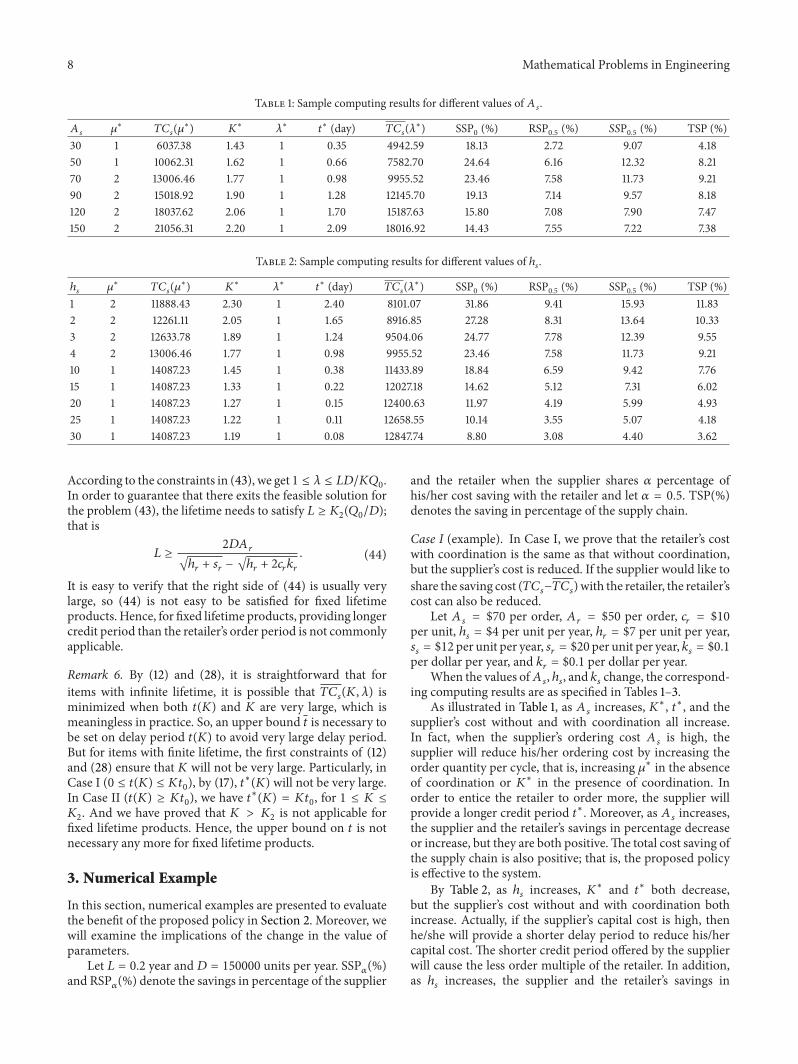
Table 1: Sample computing results for different values of 𝐴𝑠.

𝐴𝑠

𝜇∗

𝑇𝐶𝑠(𝜇∗) 𝐾

∗𝜆∗

𝑡∗ (day) 𝑇𝐶

𝑠(𝜆∗) SSP

0(%) RSP

0.5(%) 𝑆𝑆P

0.5(%) TSP (%)

30 1 6037.38 1.43 1 0.35 4942.59 18.13 2.72 9.07 4.1850 1 10062.31 1.62 1 0.66 7582.70 24.64 6.16 12.32 8.2170 2 13006.46 1.77 1 0.98 9955.52 23.46 7.58 11.73 9.2190 2 15018.92 1.90 1 1.28 12145.70 19.13 7.14 9.57 8.18120 2 18037.62 2.06 1 1.70 15187.63 15.80 7.08 7.90 7.47150 2 21056.31 2.20 1 2.09 18016.92 14.43 7.55 7.22 7.38

Table 2: Sample computing results for different values of ℎ𝑠.

ℎ𝑠

𝜇∗

𝑇𝐶𝑠(𝜇∗) 𝐾

∗𝜆∗


𝑠(𝜆∗) SSP0 (%) RSP0.5 (%) SSP0.5 (%) TSP (%)

1 2 11888.43 2.30 1 2.40 8101.07 31.86 9.41 15.93 11.832 2 12261.11 2.05 1 1.65 8916.85 27.28 8.31 13.64 10.333 2 12633.78 1.89 1 1.24 9504.06 24.77 7.78 12.39 9.554 2 13006.46 1.77 1 0.98 9955.52 23.46 7.58 11.73 9.2110 1 14087.23 1.45 1 0.38 11433.89 18.84 6.59 9.42 7.7615 1 14087.23 1.33 1 0.22 12027.18 14.62 5.12 7.31 6.0220 1 14087.23 1.27 1 0.15 12400.63 11.97 4.19 5.99 4.9325 1 14087.23 1.22 1 0.11 12658.55 10.14 3.55 5.07 4.1830 1 14087.23 1.19 1 0.08 12847.74 8.80 3.08 4.40 3.62

According to the constraints in (43), we get 1 ≤ 𝜆 ≤ 𝐿𝐷/𝐾𝑄0.

In order to guarantee that there exits the feasible solution forthe problem (43), the lifetime needs to satisfy 𝐿 ≥ 𝐾

2(𝑄0/𝐷);

that is

𝐿 ≥2𝐷𝐴𝑟

√ℎ𝑟+ 𝑠𝑟− √ℎ𝑟+ 2𝑐𝑟𝑘𝑟

. (44)

It is easy to verify that the right side of (44) is usually verylarge, so (44) is not easy to be satisfied for fixed lifetimeproducts. Hence, for fixed lifetime products, providing longercredit period than the retailer’s order period is not commonlyapplicable.

Remark 6. By (12) and (28), it is straightforward that foritems with infinite lifetime, it is possible that 𝑇𝐶

𝑠(𝐾, 𝜆) is

minimized when both 𝑡(𝐾) and 𝐾 are very large, which ismeaningless in practice. So, an upper bound 𝑡 is necessary tobe set on delay period 𝑡(𝐾) to avoid very large delay period.But for items with finite lifetime, the first constraints of (12)and (28) ensure that 𝐾 will not be very large. Particularly, inCase I (0 ≤ 𝑡(𝐾) ≤ 𝐾𝑡

0), by (17), 𝑡∗(𝐾) will not be very large.

In Case II (𝑡(𝐾) ≥ 𝐾𝑡0), we have 𝑡

∗(𝐾) = 𝐾𝑡

0, for 1 ≤ 𝐾 ≤

𝐾2. And we have proved that 𝐾 > 𝐾

2is not applicable for

fixed lifetime products. Hence, the upper bound on 𝑡 is notnecessary any more for fixed lifetime products.

3. Numerical Example

In this section, numerical examples are presented to evaluatethe benefit of the proposed policy in Section 2. Moreover, wewill examine the implications of the change in the value ofparameters.

Let 𝐿 = 0.2 year and 𝐷 = 150000 units per year. SSP𝛼(%)

and RSP𝛼(%) denote the savings in percentage of the supplier

and the retailer when the supplier shares 𝛼 percentage ofhis/her cost saving with the retailer and let 𝛼 = 0.5. TSP(%)

denotes the saving in percentage of the supply chain.

Case I (example). In Case I, we prove that the retailer’s costwith coordination is the same as that without coordination,but the supplier’s cost is reduced. If the supplier would like toshare the saving cost (𝑇𝐶

𝑠−𝑇𝐶𝑠)with the retailer, the retailer’s

cost can also be reduced.Let 𝐴

𝑠= $70 per order, 𝐴

𝑟= $50 per order, 𝑐

𝑟= $10

per unit, ℎ𝑠= $4 per unit per year, ℎ

𝑟= $7 per unit per year,

𝑠𝑠= $12 per unit per year, 𝑠

𝑟= $20 per unit per year, 𝑘

𝑠= $0.1

per dollar per year, and 𝑘𝑟= $0.1 per dollar per year.

When the values of𝐴𝑠, ℎ𝑠, and 𝑘

𝑠change, the correspond-

ing computing results are as specified in Tables 1–3.As illustrated in Table 1, as 𝐴

𝑠increases, 𝐾∗, 𝑡∗, and the

supplier’s cost without and with coordination all increase.In fact, when the supplier’s ordering cost 𝐴

𝑠is high, the

supplier will reduce his/her ordering cost by increasing theorder quantity per cycle, that is, increasing 𝜇

∗ in the absenceof coordination or 𝐾

∗ in the presence of coordination. Inorder to entice the retailer to order more, the supplier willprovide a longer credit period 𝑡

∗. Moreover, as 𝐴𝑠increases,

the supplier and the retailer’s savings in percentage decreaseor increase, but they are both positive.The total cost saving ofthe supply chain is also positive; that is, the proposed policyis effective to the system.

By Table 2, as ℎ𝑠increases, 𝐾

∗ and 𝑡∗ both decrease,

but the supplier’s cost without and with coordination bothincrease. Actually, if the supplier’s capital cost is high, thenhe/she will provide a shorter delay period to reduce his/hercapital cost. The shorter credit period offered by the supplierwill cause the less order multiple of the retailer. In addition,as ℎ𝑠increases, the supplier and the retailer’s savings in


Table 3: Sample computing results for different values of 𝑘𝑠.

𝑘𝑠

𝜇∗

𝐾∗

𝜆∗


𝑠(𝜆∗) SSP0 (%) RSP0.5 (%) SSP0.5 (%) TSP (%)

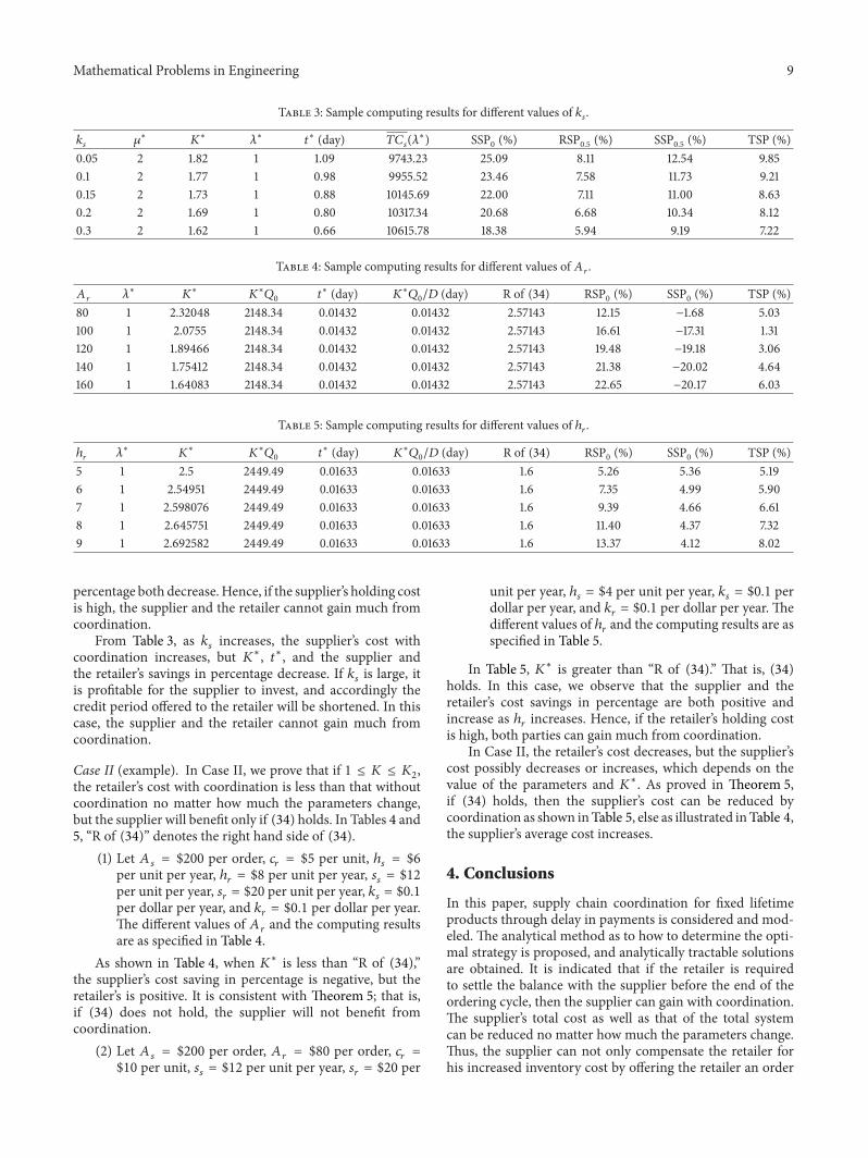
0.05 2 1.82 1 1.09 9743.23 25.09 8.11 12.54 9.850.1 2 1.77 1 0.98 9955.52 23.46 7.58 11.73 9.210.15 2 1.73 1 0.88 10145.69 22.00 7.11 11.00 8.630.2 2 1.69 1 0.80 10317.34 20.68 6.68 10.34 8.120.3 2 1.62 1 0.66 10615.78 18.38 5.94 9.19 7.22

Table 4: Sample computing results for different values of 𝐴𝑟.

𝐴𝑟

𝜆∗

𝐾∗

𝐾∗𝑄0

𝑡∗ (day) 𝐾

∗𝑄0/𝐷 (day) R of (34) RSP0 (%) SSP0 (%) TSP (%)

80 1 2.32048 2148.34 0.01432 0.01432 2.57143 12.15 −1.68 5.03100 1 2.0755 2148.34 0.01432 0.01432 2.57143 16.61 −17.31 1.31120 1 1.89466 2148.34 0.01432 0.01432 2.57143 19.48 −19.18 3.06140 1 1.75412 2148.34 0.01432 0.01432 2.57143 21.38 −20.02 4.64160 1 1.64083 2148.34 0.01432 0.01432 2.57143 22.65 −20.17 6.03

Table 5: Sample computing results for different values of ℎ𝑟.

ℎ𝑟

𝜆∗

𝐾∗

𝐾∗𝑄0

𝑡∗ (day) 𝐾

∗𝑄0/𝐷 (day) R of (34) RSP0 (%) SSP0 (%) TSP (%)

5 1 2.5 2449.49 0.01633 0.01633 1.6 5.26 5.36 5.196 1 2.54951 2449.49 0.01633 0.01633 1.6 7.35 4.99 5.907 1 2.598076 2449.49 0.01633 0.01633 1.6 9.39 4.66 6.618 1 2.645751 2449.49 0.01633 0.01633 1.6 11.40 4.37 7.329 1 2.692582 2449.49 0.01633 0.01633 1.6 13.37 4.12 8.02

percentage both decrease.Hence, if the supplier’s holding costis high, the supplier and the retailer cannot gain much fromcoordination.

From Table 3, as 𝑘𝑠increases, the supplier’s cost with

coordination increases, but 𝐾∗, 𝑡∗, and the supplier and

the retailer’s savings in percentage decrease. If 𝑘𝑠is large, it

is profitable for the supplier to invest, and accordingly thecredit period offered to the retailer will be shortened. In thiscase, the supplier and the retailer cannot gain much fromcoordination.

Case II (example). In Case II, we prove that if 1 ≤ 𝐾 ≤ 𝐾2,

the retailer’s cost with coordination is less than that withoutcoordination no matter how much the parameters change,but the supplier will benefit only if (34) holds. In Tables 4 and5, “R of (34)” denotes the right hand side of (34).

(1) Let 𝐴𝑠= $200 per order, 𝑐

𝑟= $5 per unit, ℎ

𝑠= $6

per unit per year, ℎ𝑟= $8 per unit per year, 𝑠

𝑠= $12

per unit per year, 𝑠𝑟= $20 per unit per year, 𝑘

𝑠= $0.1

per dollar per year, and 𝑘𝑟= $0.1 per dollar per year.

The different values of 𝐴𝑟and the computing results

are as specified in Table 4.As shown in Table 4, when 𝐾

∗ is less than “R of (34),”the supplier’s cost saving in percentage is negative, but theretailer’s is positive. It is consistent with Theorem 5; that is,if (34) does not hold, the supplier will not benefit fromcoordination.

(2) Let 𝐴𝑠= $200 per order, 𝐴

𝑟= $80 per order, 𝑐

𝑟=

$10 per unit, 𝑠𝑠= $12 per unit per year, 𝑠

𝑟= $20 per

unit per year, ℎ𝑠= $4 per unit per year, 𝑘

𝑠= $0.1 per

dollar per year, and 𝑘𝑟= $0.1 per dollar per year. The

different values of ℎ𝑟and the computing results are as

specified in Table 5.

In Table 5, 𝐾∗ is greater than “R of (34).” That is, (34)holds. In this case, we observe that the supplier and theretailer’s cost savings in percentage are both positive andincrease as ℎ

𝑟increases. Hence, if the retailer’s holding cost

is high, both parties can gain much from coordination.In Case II, the retailer’s cost decreases, but the supplier’s

cost possibly decreases or increases, which depends on thevalue of the parameters and 𝐾

∗. As proved in Theorem 5,if (34) holds, then the supplier’s cost can be reduced bycoordination as shown inTable 5, else as illustrated inTable 4,the supplier’s average cost increases.

4. Conclusions

In this paper, supply chain coordination for fixed lifetimeproducts through delay in payments is considered and mod-eled. The analytical method as to how to determine the opti-mal strategy is proposed, and analytically tractable solutionsare obtained. It is indicated that if the retailer is requiredto settle the balance with the supplier before the end of theordering cycle, then the supplier can gain with coordination.The supplier’s total cost as well as that of the total systemcan be reduced no matter how much the parameters change.Thus, the supplier can not only compensate the retailer forhis increased inventory cost by offering the retailer an order


size dependent delay period, but also provide the retailer withan additional saving of 𝛼(𝑇𝐶

𝑠(𝜇∗) − 𝑇𝐶

𝑠(𝐾∗, 𝜆∗)). Here, 𝛼

is determined through negotiations between the supplier andthe retailer and is generally dependent on the existing balanceof power between them. Furthermore, it is indicated that,in this case, the retailer’s order size is larger at cooperationagainst noncooperation (𝐾 > 1). As proved in Theorem 5, ifthe retailer is permitted to settle the balance after the orderingcycle, the supplier can gain only under certain conditions. Inthis case, the credit period is equal to the ordering cycle.

In the proposed model, demand is assumed to be adeterministic constant. In fact, the demand is influencedby many factors, such as price [30], inventory level [31],advertising strategy [32], and other uncertainties or noisesfrom market; so the varying or uncertain demand functionsare more practical. However, the analysis of the models inthese cases would be more complicated and we need toanalyze the characteristics of noises first [33, 34]. Perhaps it isdifficult to obtain the analytical solutions, but one could tryto obtain the optimal numerical solutions. Anyway, furtherworks could extend the models in these ways.

Conflict of Interests

The authors declare that there is no conflict of interestsregarding the publication of this paper.

Acknowledgments

The authors gratefully acknowledge the supports from theNational Natural Science Foundation of China (71371139 and71002020), the Shanghai Pujiang Program (12PJC069), the“Shu Guang” project supported by the Shanghai Munic-ipal Education Commission and the Shanghai EducationDevelopment Foundation (13SG24), and the FundamentalResearch Funds for the Central Universities.

References

[1] J. P. Monahan, “A quantity discount pricing model to increasevendor profit,”Management Science, vol. 30, no. 6, pp. 720–726,1984.

[2] H. L. Lee andM. J. Rosenblatt, “A generalized quantity discountpricing model to increase supplier’s profits,” Management Sci-ence, vol. 32, pp. 1177–1185, 1986.

[3] H. Shin andW. C. Benton, “Quantity discount-based inventorycoordination: effectiveness and critical environmental factors,”Production and Operations Management, vol. 13, no. 1, pp. 63–76, 2004.

[4] M. Y. Jaber and I. H. Osman, “Coordinating a two-level supplychain with delay in payments and profit sharing,” Computersand Industrial Engineering, vol. 50, no. 4, pp. 385–400, 2006.

[5] L.-H. Chen and F.-S. Kang, “Integrated vendor-buyer coop-erative inventory models with variant permissible delay inpayments,” European Journal of Operational Research, vol. 183,no. 2, pp. 658–673, 2007.

[6] S. P. Sarmah, D. Acharya, and S. K. Goyal, “Coordination andprofit sharing between a manufacturer and a buyer with target

profit under credit option,” European Journal of OperationalResearch, vol. 182, no. 3, pp. 1469–1478, 2007.

[7] H. Emmons and S. M. Gilbert, “The role of returns policies inpricing and inventory decisions for catalogue goods,” Manage-ment Science, vol. 44, no. 2, pp. 276–283, 1998.

[8] I. Giannoccaro and P. Pontrandolfo, “Supply chain coordinationby revenue sharing contracts,” International Journal of Produc-tion Economics, vol. 89, no. 2, pp. 131–139, 2004.

[9] G. P. Cachon, “Supply chain coordination with contracts,” inHandbooks in Operations Research and Management Science:Supply Chain Management, A. G. Kok and S. C. Graves, Eds.,pp. 229–340, Elsevier, Amsterdam, The Netherlands, 2003.

[10] P. Kouvelis, C. Chambers, and H. Wang, “Supply chain man-agement research and production and operations management:review, trends, and opportunities,” Production and OperationsManagement, vol. 15, no. 3, pp. 449–469, 2006.

[11] S. Nahmias, “Perishable inventory theory: a review,”OperationsResearch, vol. 30, no. 4, pp. 680–708, 1982.

[12] P. M. Ghare and G. H. Schrader, “A model for exponentiallydecaying inventory system,” International Journal of ProductionResearch, vol. 21, pp. 449–460, 1963.

[13] R. P. Covert and G. C. Philip, “An EOQ model for items withWeibull distribution deterioration,” AIIE Transactions, vol. 5,no. 4, pp. 323–326, 1973.

[14] G. C. Philip, “A generalized EOQmodel for items with Weibulldistribution deterioration,” AIIE Transactions, vol. 6, no. 2, pp.159–162, 1974.

[15] A. K. Jalan, R. R. Giri, and K. S. Chaudhuri, “EOQ model foritems with Weibull distribution deterioration, shortages andtrended demand,” International Journal of Systems Science, vol.27, no. 9, pp. 851–855, 1996.

[16] P. L. Abad, “Optimal pricing and lot-sizing under conditionsof perishability and partial backordering,”Management Science,vol. 42, no. 8, pp. 1093–1104, 1996.

[17] P. L. Abad, “Optimal price and order size for a reseller underpartial backordering,” Computers and Operations Research, vol.28, no. 1, pp. 53–65, 2000.

[18] S. K. Goyal and B. C. Giri, “Recent trends in modelingof deteriorating inventory,” European Journal of OperationalResearch, vol. 134, no. 1, pp. 1–16, 2001.

[19] B. E. Fries, “Optimal ordering policy for a perishable commod-ity with fixed lifetime,” Operations Research, vol. 23, no. 1, pp.46–61, 1975.

[20] S. Nahmias, “Optimal ordering policies for perishable inven-tory,” Operations Research, vol. 23, pp. 735–749, 1975.

[21] P. Nandarkumar and T. E. Morton, “Near myopic heuristic forthe fixed life perishability problem,” Management Science, vol.39, pp. 1490–1498, 1993.

[22] L. Liu andZ. Lian, “(s, S) continuous reviewmodels for productswith fixed lifetimes,”Operations Research, vol. 47, no. 1, pp. 150–158, 1999.

[23] H. Hwang and K. H. Hahn, “An optimal procurement policy foritems with an inventory level-dependent demand rate and fixedlifetime,” European Journal of Operational Research, vol. 127, no.3, pp. 537–545, 2000.

[24] Z. Lian and L. Liu, “Continuous review perishable inventorysystems: models and heuristics,” IIE Transactions, vol. 33, no.9, pp. 809–822, 2001.

[25] E. Berk and U. Gurler, “Analysis of the (Q, r) inventorymodel for perishables with positive lead times and lost sales,”Operations Research, vol. 56, no. 5, pp. 1238–1246, 2008.


[26] F. Olsson and P. Tydesjo, “Inventory problems with perishableitems: fixed lifetimes and backlogging,” European Journal ofOperational Research, vol. 202, no. 1, pp. 131–137, 2010.

[27] Y. Duan, J. Luo, and J. Huo, “Buyer-vendor inventory coordina-tionwith quantity discount incentive for fixed lifetime product,”International Journal of Production Economics, vol. 128, no. 1, pp.351–357, 2010.

[28] Y. Duan, J. Huo, Y. Zhang, and J. Zhang, “Two level supplychain coordination with delay in payments for fixed lifetimeproducts,” Computers & Industrial Engineering, vol. 63, no. 2,pp. 456–463, 2012.

[29] H. Hwang and K. H. Hahn, “Optimal procurement policy foritems with an inventory level-dependent demand rate and fixedlifetime,” European Journal of Operational Research, vol. 127, no.3, pp. 537–545, 2000.

[30] J.-T. Teng, C.-T. Chang, and S. K. Goyal, “Optimal pricingand ordering policy under permissible delay in payments,”International Journal of Production Economics, vol. 97, no. 2, pp.121–129, 2005.

[31] T. L. Urban, “Inventorymodels with inventory-level-dependentdemand: a comprehensive review and unifying theory,” Euro-pean Journal of Operational Research, vol. 162, no. 3, pp. 792–804, 2005.

[32] N. H. Shah, H. N. Soni, and K. A. Patel, “Optimizing inventoryandmarketing policy for non-instantaneous deteriorating itemswith generalized type deterioration and holding cost rates,”Omega, vol. 41, pp. 421–430, 2013.

[33] M. Li andW. Zhao, “On bandlimitedness and lag-limitedness offractional Gaussian noise,” Physica A, vol. 392, no. 9, pp. 1955–1961, 2013.

[34] M. Li, “A class of negatively fractal dimensional gaussianrandom functions,”Mathematical Problems in Engineering, vol.2011, Article ID 291028, 18 pages, 2011.

Submit your manuscripts athttp://www.hindawi.com

Hindawi Publishing Corporationhttp://www.hindawi.com Volume 2014

MathematicsJournal of


Mathematical Problems in Engineering

Hindawi Publishing Corporationhttp://www.hindawi.com

Differential EquationsInternational Journal of

Volume 2014

Applied MathematicsJournal of


Probability and StatisticsHindawi Publishing Corporationhttp://www.hindawi.com Volume 2014

Journal of


Mathematical PhysicsAdvances in

Complex AnalysisJournal of


OptimizationJournal of


CombinatoricsHindawi Publishing Corporationhttp://www.hindawi.com Volume 2014

International Journal of


Operations ResearchAdvances in

Journal of


Function Spaces

Abstract and Applied AnalysisHindawi Publishing Corporationhttp://www.hindawi.com Volume 2014

International Journal of Mathematics and Mathematical Sciences


The Scientific World JournalHindawi Publishing Corporation http://www.hindawi.com Volume 2014


Algebra

Discrete Dynamics in Nature and Society



Decision SciencesAdvances in

Discrete MathematicsJournal of

Hindawi Publishing Corporationhttp://www.hindawi.com

Volume 2014 Hindawi Publishing Corporationhttp://www.hindawi.com Volume 2014

Stochastic AnalysisInternational Journal of

Documents

Research Article Supply Chain Coordination for …downloads.hindawi.com/journals/mpe/2014/649189.pdf · Research Article Supply Chain Coordination for Fixed Lifetime Products with