Embed Size (px)
Citation preview

Research ArticleSimple Model for Simulating Characteristics ofRiver Flow Velocity in Large Scale
Husin Alatas12 Dyo D Prayuda2 Achmad Syafiuddin2 May Parlindungan3
Nurjaman O Suhendra3 and Hidayat Pawitan13
1Research Cluster for Dynamics and Modeling of Complex Systems Faculty of Mathematics and Natural SciencesBogor Agricultural University Jl Meranti Kampus IPB Darmaga Bogor 16680 Indonesia2Theoretical Physics Division Department of Physics Bogor Agricultural University Jl Meranti Kampus IPB DarmagaBogor 16680 Indonesia3Hydrometeorology Division Department of Geophysics and Meteorology Bogor Agricultural University Jl MerantiKampus IPB Darmaga Bogor 16680 Indonesia
Correspondence should be addressed to Husin Alatas alatasipbacid and Hidayat Pawitan hpawitanipbacid
Received 28 July 2014 Accepted 30 December 2014
Academic Editor Alexey Stovas
Copyright copy 2015 Husin Alatas et al This is an open access article distributed under the Creative Commons Attribution Licensewhich permits unrestricted use distribution and reproduction in any medium provided the original work is properly cited
We propose a simple computer based phenomenological model to simulate the characteristics of river flow velocity in large scaleWe use shuttle radar tomography mission based digital elevation model in grid form to define the terrain of catchment area Themodel relies on mass-momentum conservation law and modified equation of motion of falling body in inclined plane We assumeinelastic collision occurs at every junction of two river branches to describe the dynamics of merged flow velocity
1 Introduction
The complexity of river network has been studied intensivelyover the past decades in order to describe its pattern forma-tion and dynamics [1]The evolution of river network patternhas been investigated based on various approaches such ascontinuum [2ndash4] stochastic [5] and cellular [6] approachesOn the other hand one of the most important dynamicalcharacteristics of a river is its flow velocity which correspondsto the water discharge along the river lines Many differentempirical models have been proposed to describe the asso-ciated dynamics in various scales and for various purposesas well [7ndash12] Recently Gauckler-Manning-Strickler (GMS)formula based empirical model has been implemented todescribe the global river flow in certain area of Europe [9]
In the meantime one of the theoretical descriptions ofdynamics of openclose river channel is given by the so-calledSaint Venant equations (SVEs) in one or two dimensionsThese spatiotemporal equations are developed on the basisof mass-momentum conservation law in the form of coupledcontinuity and momentum differential equations of average
water discharge and cross-sectional river flow channel func-tions where both need initial and boundary conditions [7 13ndash19] Recently one-dimensional SVE has been adopted in acoupled hydrodynamic analysismodel to investigate the largescale water discharge dynamics at basin of Yangtze RiverChina in the presence of complex river-lake interaction [7]
In general the river flow dynamics is affected by frictionroughness slope and number of rocks Usually in SVEs allthese parameters are incorporated in theGMS formula whichis found empirically to approximate the average flow velocityin short distance [17] However solving SVEs to simulate theriver flow dynamics in a large scale such as the whole area ofcatchment area is not an easy task It can be done by solvingeither the two-dimensional SVE or the one-dimensionalSVE incorporated by junction model with internal boundaryconditions [7 19 20] It is likely that for large scale casesthe calculation to solve the related SVEs based on rigoroussemianalytical or numericalmethods can be very difficult andprobably time consuming One of the difficult challenges tosolve these equations numerically for the corresponding casesis how to determine the corresponding initial conditions [7]
Hindawi Publishing CorporationInternational Journal of GeophysicsVolume 2015 Article ID 520893 8 pageshttpdxdoiorg1011552015520893
2 International Journal of Geophysics
Katulampa
4
3 1
2
5
(a)
331 319 317 322 328 334 339 341 345 353 354313 314 323 321 325 331 337 341 345 351 357343 342 315 316 317 318 331 337 343 348 356345 345 316 336 333 326 322 335 340 343 348347 349 336 343 346 342 335 323 324 327 344348 350 340 347 350 353 353 350 345 340 329348 351 342 342 353 357 358 358 358 358 351350 351 354 355 343 356 361 362 363 366 366351 353 356 358 358 344 362 362 364 367 370350 353 357 360 362 347 363 365 365 367 372344 347 351 359 366 365 352 355 367 369 373
(b)
Figure 1 (a) The network pattern of Ciliwung River catchment area which is divided into five regions The solid dot represents the positionof Katulampa observation point (b) Modified DEM data of 90 times 90m2 grid resolution of a small area around Katulampa
In this report we propose a simple approach to developa computer based discrete phenomenological model of riverflow velocity We still rely on mass-momentum conservationlaw by assuming that an inelastic collision occurs at a riverjunction Instead of using GMS formula to accommodatefriction roughness and number of rocks in single param-eter here we introduce the notion of effective gravitationalacceleration whereas the flow velocity follows the equationof motion of falling body in inclined plane
The procedure that we followed to develop the modelincludes the following (i) determination of river catchmentarea in the form of a computational window grid (ii)development of algorithm for flow velocity model and (iii)examining the model characteristics with respect to thevariations of initial water discharges at headwaters
To our best knowledge the proposed model has neverbeen reported elsewhere We compare our model with fieldobservation data in order to justify the results It should beemphasized from the beginning that this simple model isan attempt to determine characteristics of river flow velocityand it is not intended to replace SVEs In principle howeverthis model can also provide initial condition of the wholeriver network which is needed to solve numerically thecorresponding time-dependent SVEs
We considered the catchment area of CiliwungRiver (CR)situated in West Java Province Indonesia for simulating themodel To define the corresponding terrain we used digitalelevation model (DEM) in grid form which is constructedbased on free shuttle radar topography mission (SRTM) dataprovided by USGS [20] Each grid in DEM represents theaverage heightwithin the corresponding terrainWeonly takeinto account the surface runoff and exclude the subsurfacerunoff as well as landscape characteristics of surroundingriver lines such as forest canopy vegetation land use andsediment transport
We organize this report as follows in Section 2 we discussthe associated DEM of CR catchment area and then thisis followed by the explanation of flow velocity model inSection 3The results of our simulation and its discussion aregiven in Section 4 We conclude our report by a summary in
Section 5 Sections 2ndash4 discuss consecutively the abovemen-tioned procedure that we followed
2 DEM of Ciliwung River Catchment Area
The CR is one of the most important rivers in Java IslandIndonesia It spans over 120 km from Mount Pangrango inWest Java to Java Sea north to the capital city Jakarta Itscatchment area is 149 km2 In recent years during the rainyseason this river contributes around 30 of flood in Jakarta
To plot the CR catchment area we used DEM with 90 times90m2 grid resolution and in order to get a more detailedterrain which still can be handled by modest computationalfacility the associated DEM was corrected by 15 times 15m2resolution DEM as well as data from field survey Using GISsoftware this modified DEM was converted into numbersthat can be read by Excel software Shown in Figure 1(a)is the plot of 90 times 90m2 DEM of the corresponding CRriver network pattern It is obvious that water will flow tothe lower land due to gravitational force such that we canuse this fact as a rule in our computer code to determinethe corresponding river pattern based on the given DEMdata after identifying the positions of all headwaters There-fore it is clear that the boundaries of all river brancheswhich define a two-dimensional computational window areautomatically provided by DEM where each grid representsthe corresponding computational mesh In Figure 1(b) wegive an example of specific small area of the correspondingcomputational window grid (see figure caption) which ishighlightedwith grey color gridThe number inside each gridrepresents DEM value in meter unit at specific position
Based on our modified DEM we identified that thereare 126 headwaters According to Strahler classification ofriver branches all these headwaters converge into order 4river channel at Katulampa area with channel dimension ofsim70mwidth and 03ndash05mwater level Similar to the most oftropical rivers catchment upper area of CR is also filled up byrocks with relatively large size
International Journal of Geophysics 3
3 Flow Velocity Model
We consider a discrete model where the water dischargeis represented by the corresponding two-dimensional gridin the modified DEM in which its position is denoted byindices (119894 119895) After determining the river network pattern wemodel the corresponding flow velocity by assuming that itsmagnitude at particular position of water discharge along ariver channel is given by the following equation
V (119894 119895) = radicV2 (1198941015840 1198951015840) + 2119892eff (1198941015840 1198951015840 ℎ) Δ119867 (1)
where V(1198941015840 1198951015840) and V(119894 119895) denote the flow velocity of waterdischarge at higher and lower positions respectively whileΔ119867 = 119867(119894
1015840 1198951015840) minus 119867(119894 119895) gt 0 is the height (119867) difference
where the value of 119867 is provided by DEM The symbol 119892effrepresents the effective gravitational acceleration which isdefined to accommodate the real condition of river channelsand ℎdenoteswater level from river bed at the position (1198941015840 1198951015840)Flow velocities in (1) can be interpreted as the average ofvelocity in the associated grid In themeantime thewidth andwater level of each river branch are assumed to be uniform
In general we assume that the parameter 119892eff depends onposition andwater level which can be determined empiricallythrough field observation at particular time The assumptionof water level dependency is taken to accommodate the factthat water flow is more efficient as water level increases Butfor the sake of simplicity here we assume that 119892eff is uniformalong all river channels and it will be determined laternumerically Comparing with the flow velocity expression inGMS formula this parameter plays similar role with the ratio11987723
119867119899 where 119877
119867is hydraulic radius of a river channel and 119899
represents roughness coefficient [9]Next to model the merging of flows from two dif-
ferent branches at a river junction we assume that thecollision of water at each junction is inelastic satisfying themass-momentum conservation law in the following discretenumerical scheme
1198763(119894 119895) = 119876
1(119894 119895) + 119876
2(119894 119895) (2)
3(119894 119895) =
1(119894 119895) +
2(119894 119895) (3)
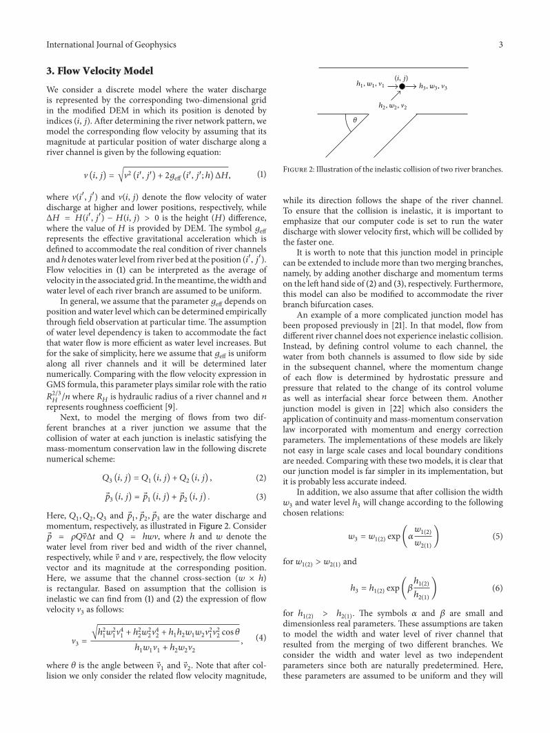
Here 1198761 1198762 1198763and
1 2 3are the water discharge and
momentum respectively as illustrated in Figure 2 Consider = 120588119876VΔ119905 and 119876 = ℎ119908V where ℎ and 119908 denote thewater level from river bed and width of the river channelrespectively while V and V are respectively the flow velocityvector and its magnitude at the corresponding positionHere we assume that the channel cross-section (119908 times ℎ)is rectangular Based on assumption that the collision isinelastic we can find from (1) and (2) the expression of flowvelocity V
3as follows
V3=
radicℎ2
11199082
1V41+ ℎ2
21199082
2V42+ ℎ1ℎ211990811199082V21V22cos 120579
ℎ11199081V1+ ℎ21199082V2
(4)
where 120579 is the angle between V1and V
2 Note that after col-
lision we only consider the related flow velocity magnitude
h1 w1 1
h2 w2 2
h3 w3 3
120579
(i j)
Figure 2 Illustration of the inelastic collision of two river branches
while its direction follows the shape of the river channelTo ensure that the collision is inelastic it is important toemphasize that our computer code is set to run the waterdischarge with slower velocity first which will be collided bythe faster one
It is worth to note that this junction model in principlecan be extended to include more than twomerging branchesnamely by adding another discharge and momentum termson the left hand side of (2) and (3) respectively Furthermorethis model can also be modified to accommodate the riverbranch bifurcation cases
An example of a more complicated junction model hasbeen proposed previously in [21] In that model flow fromdifferent river channel does not experience inelastic collisionInstead by defining control volume to each channel thewater from both channels is assumed to flow side by sidein the subsequent channel where the momentum changeof each flow is determined by hydrostatic pressure andpressure that related to the change of its control volumeas well as interfacial shear force between them Anotherjunction model is given in [22] which also considers theapplication of continuity and mass-momentum conservationlaw incorporated with momentum and energy correctionparameters The implementations of these models are likelynot easy in large scale cases and local boundary conditionsare needed Comparing with these two models it is clear thatour junction model is far simpler in its implementation butit is probably less accurate indeed
In addition we also assume that after collision the width1199083and water level ℎ
3will change according to the following
chosen relations
1199083= 1199081(2)
exp(1205721199081(2)
1199082(1)
) (5)
for 1199081(2)gt 1199082(1)
and
ℎ3= ℎ1(2)
exp(120573ℎ1(2)
ℎ2(1)
) (6)
for ℎ1(2)gt ℎ2(1)
The symbols 120572 and 120573 are small anddimensionless real parameters These assumptions are takento model the width and water level of river channel thatresulted from the merging of two different branches Weconsider the width and water level as two independentparameters since both are naturally predetermined Herethese parameters are assumed to be uniform and they will
4 International Journal of Geophysics
be determined numerically In general however one mightconsider that their values should not be the same for differentjunction and can be determined empirically Indeed one canchoose another type of relation to model the width 119908
3and
water level ℎ3 However based on our numerical experiment
which will be presented in the next section the relationsgiven by (5) and (6) so far are the most applicable ones tomeet the corresponding river parameters and certainly thisassumption must be further clarified by field observationwhich is beyond the scope of this report
To this end it is well known that based on the followingdefinition of Froude number for a channel with rectangularcross-section
Fr = Vradic119892 times ℎ (7)
where 119892 is the actual gravitational acceleration one canclassify the flow regimes into subcritical (Fr lt 1) critical(Fr = 1) and supercritical (Fr gt 1) flow [23] It willbe discussed on the next section that the model seems toaccommodate only the case of subcritical flow
4 Results of Model Simulation and Discussion
To simulate our model we use the water discharge datasample found from our field surveys during dry seasonin August 2013 Based on those data samples we considerdividing the 126 headwaters into five regions and chooseKatulampa as the simulation point as shown in Figure 1(b)The corresponding data of headwaters and Katulampa pointwere considered as the associated initial and final conditionsrespectively
The initial flow velocity width and water level fromfield survey in each region are assumed to be uniform asgiven in Table 1 Prior to discussing the characteristics ofour model with respect to the initial flow velocity and waterlevel variations we first simulate the flow velocity water leveland width at Katulampa with initial values given in Table 1Our simulation yields the following results V = 094msℎ = 041m and 119908 = 7001m On the other hand fromfield survey we observed the following data V asymp 090msℎ asymp 05m and 119908 asymp 6063m To meet the simulation resultsthat match Katulampa data we adjusted by trial and error theparameters in (1) (5) and (6) and found the following values119892eff = 9times10
minus5ms2120572 = 63times10minus3 and120573 = 55times10minus3 whereasin our computer code we run the initial water discharge fromregion 1 first and then from regions 2 3 4 and 5 respectivelysince V
01lt V02lt V03lt V04lt V05 It is worth to note that
by assuming 119892 sim 981ms2 all these velocities at headwatersand Katulampa are related to subcritical flows according toFroude number given by (7)
The simulation results of flow velocity water level andwidth of thewhole catchment area of CR are given in Figure 3Comparing to our data sample the simulated flow velocitywidth and water level do not represent most of the actualconditions although at Katulampa these quantities are ingood agreement This can be explained as a consequenceof not applying actual data of the whole headwaters to our
Table 1 Initial flow velocity (V0) width (119908
0) and water level (ℎ
0) of
each chosen region
Region V0(ms) 119908
0(m) ℎ
0(m)
1 0342 485 0202 0429 312 0103 0437 181 0304 0527 155 0305 0940 277 040
model One might expect that the use of actual data of allheadwaters and considering position-dependent 119892eff 120572 and120573will give fairly accurate results with tolerable deviations Asshown in Figure 3(a) it is found that at every river branchjunction the flow velocity of merged water discharge isgetting slower due to inelastic collision given by (3) whichcorresponds to kinetic energy losses phenomenon
Next to simulate the characteristics of flow velocity atKatulampa we vary the initial flow velocity at headwater ofparticular region while keeping the velocity of other regionsthe same Given in Table 2 are five different variations ofthe first one denoted by letters A B C D and E with thecorresponding results depicted in Figure 4 In variation Awe vary the initial flow velocity V
01= 0ndash04290ms It is
found that the flow velocity at Katulampa exhibits nonlinearvariation as shown in Figure 4(a) However it should benoted that the change is relatively small In contrast asshown in Figure 4(b) we observe for variation B whereV02= 03420ndash04290ms variation is considered that the
flow velocity at Katulampa does not vary at all On theother hand the other different characteristics are foundfor variations C and D with the corresponding variationsgiven as follows V
03= 04290ndash05270ms and V
04=
04370ndash09400ms respectively As shown in Figures 4(c)and 4(d) both variations exhibit opposite characteristicswhere in variation C the flow velocity is increasing almostlinearly while for variation D the flow velocity is decreasinglinearly In the meantime the variation E given in Figure 4(e)is similar to variation A where its variation is nonlinear withrespect to the linear variation of initial flow velocity V
05=
05270ndash14msFor comparison we also consider another five variations
of the second one denoted by letters F G H I and J withthe corresponding variations of initial flow velocity of eachregion given in Table 3 Here we exchange the initial flowvelocity between region 4 and region 5 such that V
04gt V05
The results are depicted in Figure 5 Comparing variationsA B and C and variations F G and H of Figures 4(a)ndash4(c) and Figures 5(a)ndash5(c) respectively we see that similarcharacteristics are exhibited for variations of regions 1 2 and3 respectively but with different flow velocity magnitudesInterestingly this similarity is not the case for variations Iand J given in Figures 5(d) and 5(e) respectively where bothvariations demonstrate flat characteristics These results arein contrast to the previous variationsD and E given in Figures4(d) and 4(e)
International Journal of Geophysics 5
14
12
02
0
1
08
06
04
(ms)
(a)
03
02
01
0
04
(m)
(b)
(m)
60
40
20
0
(c)
Figure 3 Global pattern of (a) flow velocity (b) water level and (c) width In these figures we set to zero all the corresponding values outsidethe river channels
Table 2 First variation of initial flow velocity
Variation V01
(ms) V02
(ms) V03
(ms) V04
(ms) V05
(ms)A 0ndash04290 04290 04370 05270 09400B 03420 03420ndash04370 04370 05270 09400C 03420 04290 04290ndash05270 05270 09400D 03420 04290 04370 04370ndash09400 09400E 03420 04290 04370 05270 05270ndash14
To complete our investigation on the flow velocity char-acteristics at Katulampa with respect to initial flow velocityvariation we also simulate themodel by uniformly increasingthe value of initial flow velocity of each regionThe results aregiven in Figure 6 showing nonlinear variation of velocity atKatulampawith respect to the uniform increment of all initialflow velocities by ΔV
0
Clearly since it is considered that the water level does notvary and that the related velocity at Katulampa tends to growexponentially then the corresponding Froude number at thatpoint which is given by (7) can probably be of Fr ≫ 1Therefore based on this fact it is safe to say that our modelmost likely cannot describe the supercritical flow in a fairlyaccurate way
All these results obviously indicate that the influenceof initial flow velocity variation at headwaters will leadto specific characteristics of flow velocity at lower landHowever the associated characteristics cannot be easilyexplained due to complex interaction under inelastic collisionamong the corresponding river branches This situation canbe exemplified by the nonlinear characteristic of variation E
which is clearly different compared to variation I with flatcharacteristic although both variations have the same initialflow velocity variation on the related region (05270ndash14ms)and the location of the corresponding headwaters is relativelyclose to Katulampa as shown in Figure 1
We have discussed previously in Section 3 that in generalthe parameter 119892eff depends on water level Therefore inaddition to the aforementioned variations we have alsoinvestigated the characteristics of flowvelocity andwater levelat Katulampa by increasing linearly the water level of eachheadwater as follows
ℎ (Δℎ) = ℎ0[1 +Δℎ
ℎ0
] (8)
with Δℎ = 01 times 119899m where 119899 is an integer In the mean-time the effective gravitational acceleration is considered toincrease linearly based on the following equation
119892eff (Δℎ) = 119892eff (0) [1 +Δℎ
ℎ0
] (9)
6 International Journal of Geophysics
0 0050 0150 0250 0350 045009200
09300
09400
09500k(m
s)
01 (ms)
(a)
0340 0360 0380 0400 0420 044009200
09300
09400
09500
k(m
s)
02 (ms)
(b)
0430 0450 0470 0490 0510 053009200
09300
09400
09500
k(m
s)
03 (ms)
(c)
0420 0520 0620 0720 0820 092009200
09300
09400
09500
k(m
s)
04 (ms)
(d)
05 5 10 1509200
09300
09400
09500
05 (ms)
k(m
s)
(e)
Figure 4 Characteristics of flow velocity at Katulampa with respect to the first variation of initial flow speed (a) A (b) B (c) C (d) D and(e) E
Table 3 Second variation of initial flow velocity
Variation V01
(ms) V02
(ms) V03
(ms) V04
(ms) V05
(ms)F 0ndash04290 04290 04370 09400 05270G 03420 03420ndash04370 04370 09400 05270H 03420 04290 04290ndash05270 09400 05270I 03420 04290 04370 05270ndash14 05270J 03420 04290 04370 09400 04370ndash09400
which is taken under the assumption that higher water levelwill flowmore easily Here ℎ
0is given in Table 1The result is
shown in Figure 7 It is found that the flow velocity variationat Katulampa increases nonlinearly with tendency of satura-tion while the corresponding water level increases linearly
Finally it should be admitted that our simple modelmust be further examined by field observation which shouldbe conducted in relatively long time period However thismodel can be used to determine and predict qualitatively thecharacteristics of river flow velocity in large scale In additionfor a relatively small grid DEM in principle the calculated
velocity water level andwidth can be used as initial conditionof time-dependent SVEs
5 Summary
We have discussed our simple computer based model forsimulating the river flow velocity We consider CiliwungRiver as the area of simulation where the correspond-ing digital elevation model (DEM) is based on SRTMdata from USGS with 90 times 90m2 resolution and mod-ified by 15 times 15m2 as well as data from field survey
International Journal of Geophysics 7
0 0050 0150 0250 0350 045009200
09300
09400
09500
01 (ms)
k(m
s)
(a)
0340 0360 0380 0400 0420 044009200
09300
09400
09500
k(m
s)
02 (ms)
(b)
0430 0450 0470 0490 0510 053009200
09300
09400
09500
k(m
s)
03 (ms)
(c)
05 5 10 1509200
09300
09400
09500
k(m
s)
04 (ms)
(d)
0420 0520 0620 0720 0820 092009200
09300
09400
09500
k(m
s)
05 (ms)
(e)
Figure 5 Characteristics of flow velocity at Katulampa with respect to the second variation of initial flow speed (a) F (b) G (c) H (d) I and(e) J
0
0100
0200
0300
0400
0500 0
0100
0200
0300
0400
09000
09500
10000
10500
11000
11500
k(m
s)
Δ0 (ms)
Figure 6 Characteristic of flow velocity at Katulampa with respectto uniform increasing of initial flow speed of all regions
The flow velocity is described by equation of motion offalling body in inclined plane due to gravitational force
We define the effective gravitational acceleration parame-ter to accommodate the real condition of river channelAt the junction of two river branches we assume that themerged flow velocity is determined by inelastic collision Itis found that our model can determine the flow velocity atKatulampa in good agreement with observation data Thevariations of initial flow velocity of certain region in theCiliwung River headwaters show various characteristics thatwe suspect to occur due to complex interaction among theriver branches This simple model can be used to determineand predict the characteristics of river flow velocity atsubcritical level as well as providing an initial condition fortime-dependent Saint Venant equations
Conflict of Interests
The authors declare that there is no conflict of interestsregarding the publication of this paper
8 International Journal of Geophysics
0 02 04 06 08 1 12 14 16 18 2
1
2
3
4
5
6
Δh (m)
hk(m
)
(a)
0 02 04 06 08 1 12 14 16 18 21
2
3
4
Δh (m)
k(m
s)
(b)
Figure 7 (a) Characteristics of water level and (b) flow velocity (dashed circle) at Katulampa with respect to uniform increasing of initialwater level of all regions
Acknowledgment
This work was funded by BOPTN Research Grant of year2013 from Directorate of Higher Education Ministry ofNational Education and Culture Republic of Indonesiaunder Contract no 198IT3412L2SPK2013
References
[1] W Wu Computational River Dynamics Taylor amp FrancisLondon UK 2002
[2] A Giacometti A Maritan and J R Banavar ldquoContinuummodel for river networksrdquo Physical Review Letters vol 75 no3 pp 577ndash580 1995
[3] F Metivier ldquoDiffusivelike buffering and saturation of largeriversrdquo Physical Review E Statistical Physics Plasmas Fluidsand Related Interdisciplinary Topics vol 60 no 5 pp 5827ndash5832 1999
[4] A Giacometti ldquoLocal minimal energy landscapes in rivernetworksrdquoPhysical ReviewE vol 62 no 5 pp 6042ndash6051 2000
[5] G Yan J ZhangHWang and LGuo ldquoSimple stochastic latticegas automaton model for formation of river networksrdquo PhysicalReview E vol 78 no 6 Article ID 066102 2008
[6] G Caldarelli A Giacometti A Maritan I Rodriguez-Iturbeand A Rinaldo ldquoRandomly pinned landscape evolutionrdquo Phys-ical Review EmdashStatistical Physics Plasmas Fluids and RelatedInterdisciplinary Topics vol 55 no 5 pp R4865ndashR4868 1997
[7] X Lai J Jiang Q Liang and Q Huang ldquoLarge-scale hydro-dynamic modeling of the middle Yangtze River Basin withcomplex river-lake interactionsrdquo Journal of Hydrology vol 492pp 228ndash243 2013
[8] M E Akiner and A Akkoyunlu ldquoModeling and forecastingriver flow rate from the Melen watershed Turkeyrdquo Journal ofHydrology vol 456-457 pp 121ndash129 2012
[9] K Verzano I BarlundM Florke et al ldquoModeling variable riverflow velocity on continental scale current situation and climatechange impacts in Europerdquo Journal of Hydrology vol 424-425pp 238ndash251 2012
[10] G Steinebach S Rademacher P Rentrop and M SchulzldquoMechanisms of coupling in river flow simulation systemsrdquoJournal of Computational and AppliedMathematics vol 168 no1-2 pp 459ndash470 2004
[11] C H David Z-L Yang and S Hong ldquoRegional-scale riverflow modeling using off-the-shelf runoff products thousands
of mapped rivers and hundreds of stream flow gaugesrdquo Envi-ronmental Modelling and Software vol 42 pp 116ndash132 2013
[12] F Liu and B R Hodges ldquoApplying microprocessor analysismethods to river network modellingrdquo Environmental Modellingamp Software vol 52 pp 234ndash252 2014
[13] R Moussa and C Bocquillon ldquoApproximation zones of theSaint-Venant equations for flood routing with overbank flowrdquoHydrology and Earth System Sciences vol 4 no 2 pp 251ndash2612000
[14] R Szymkiewicz ldquoSolution of the inverse problem for the SaintVenant equationsrdquo Journal of Hydrology vol 147 no 1ndash4 pp105ndash120 1993
[15] E Blade M Gomez-Valentın J Dolz J L Aragon-HernandezG Corestein and M Sanchez-Juny ldquoIntegration of 1D and 2Dfinite volume schemes for computations of water flow in naturalchannelsrdquo Advances in Water Resources vol 42 pp 17ndash29 2012
[16] S KOoiM PM Krutzen and EWeyer ldquoOn physical and datadriven modelling of irrigation channelsrdquo Control EngineeringPractice vol 13 no 4 pp 461ndash471 2005
[17] V dos Santos Martins M Rodrigues and M Diagne ldquoA multi-model approach to Saint-Venant equations a stability studyby LMIsrdquo International Journal of Applied Mathematics andComputer Science vol 22 no 3 pp 539ndash550 2012
[18] T G Lich and L K Luat ldquoBoundary conditions for the two-dimensional Saint-Venant equation systemrdquoAppliedMathemat-ical Modelling vol 16 no 9 pp 498ndash502 1992
[19] R Ghostine R Mose J Vazquez A Ghenaim and C GregoireldquoTwo-dimensional simulation of subcritical flow at a combiningjunction luxury or necessityrdquo Journal of Hydraulic Engineeringvol 136 no 10 Article ID 004010QHY pp 799ndash805 2010
[20] httpgdexcrusgsgovgdex[21] S Shabayek P Steffler and F Hicks ldquoDynamic model for
subcritical combining flows in channel junctionsrdquo Journal ofHydraulic Engineering vol 128 no 9 pp 821ndash828 2002
[22] C CHsuW J Lee andCHChang ldquoSubcritical open-channeljunction flowrdquo Journal of Hydraulic Engineering vol 124 no 8pp 847ndash855 1998
[23] H Chanson Hydraulics of Open Channel Flow Butterworth-Heinemann Oxford UK 2004
Submit your manuscripts athttpwwwhindawicom
Hindawi Publishing Corporationhttpwwwhindawicom Volume 2014
ClimatologyJournal of
EcologyInternational Journal of
Hindawi Publishing Corporationhttpwwwhindawicom Volume 2014
EarthquakesJournal of
Hindawi Publishing Corporationhttpwwwhindawicom Volume 2014
Hindawi Publishing Corporationhttpwwwhindawicom
Applied ampEnvironmentalSoil Science
Volume 2014
Mining
Hindawi Publishing Corporationhttpwwwhindawicom Volume 2014
Journal of
Hindawi Publishing Corporation httpwwwhindawicom Volume 2014
International Journal of
Geophysics
OceanographyInternational Journal of
Hindawi Publishing Corporationhttpwwwhindawicom Volume 2014
Journal of Computational Environmental SciencesHindawi Publishing Corporationhttpwwwhindawicom Volume 2014
Journal ofPetroleum Engineering
Hindawi Publishing Corporationhttpwwwhindawicom Volume 2014
GeochemistryHindawi Publishing Corporationhttpwwwhindawicom Volume 2014
Journal of
Atmospheric SciencesInternational Journal of
Hindawi Publishing Corporationhttpwwwhindawicom Volume 2014
OceanographyHindawi Publishing Corporationhttpwwwhindawicom Volume 2014
Advances in
Hindawi Publishing Corporationhttpwwwhindawicom Volume 2014
MineralogyInternational Journal of
Hindawi Publishing Corporationhttpwwwhindawicom Volume 2014
MeteorologyAdvances in
The Scientific World JournalHindawi Publishing Corporation httpwwwhindawicom Volume 2014
Paleontology JournalHindawi Publishing Corporationhttpwwwhindawicom Volume 2014
ScientificaHindawi Publishing Corporationhttpwwwhindawicom Volume 2014
Hindawi Publishing Corporationhttpwwwhindawicom Volume 2014
Geological ResearchJournal of
Hindawi Publishing Corporationhttpwwwhindawicom Volume 2014
Geology Advances in

2 International Journal of Geophysics
Katulampa
4
3 1
2
5
(a)
331 319 317 322 328 334 339 341 345 353 354313 314 323 321 325 331 337 341 345 351 357343 342 315 316 317 318 331 337 343 348 356345 345 316 336 333 326 322 335 340 343 348347 349 336 343 346 342 335 323 324 327 344348 350 340 347 350 353 353 350 345 340 329348 351 342 342 353 357 358 358 358 358 351350 351 354 355 343 356 361 362 363 366 366351 353 356 358 358 344 362 362 364 367 370350 353 357 360 362 347 363 365 365 367 372344 347 351 359 366 365 352 355 367 369 373
(b)
Figure 1 (a) The network pattern of Ciliwung River catchment area which is divided into five regions The solid dot represents the positionof Katulampa observation point (b) Modified DEM data of 90 times 90m2 grid resolution of a small area around Katulampa
In this report we propose a simple approach to developa computer based discrete phenomenological model of riverflow velocity We still rely on mass-momentum conservationlaw by assuming that an inelastic collision occurs at a riverjunction Instead of using GMS formula to accommodatefriction roughness and number of rocks in single param-eter here we introduce the notion of effective gravitationalacceleration whereas the flow velocity follows the equationof motion of falling body in inclined plane
The procedure that we followed to develop the modelincludes the following (i) determination of river catchmentarea in the form of a computational window grid (ii)development of algorithm for flow velocity model and (iii)examining the model characteristics with respect to thevariations of initial water discharges at headwaters
To our best knowledge the proposed model has neverbeen reported elsewhere We compare our model with fieldobservation data in order to justify the results It should beemphasized from the beginning that this simple model isan attempt to determine characteristics of river flow velocityand it is not intended to replace SVEs In principle howeverthis model can also provide initial condition of the wholeriver network which is needed to solve numerically thecorresponding time-dependent SVEs
We considered the catchment area of CiliwungRiver (CR)situated in West Java Province Indonesia for simulating themodel To define the corresponding terrain we used digitalelevation model (DEM) in grid form which is constructedbased on free shuttle radar topography mission (SRTM) dataprovided by USGS [20] Each grid in DEM represents theaverage heightwithin the corresponding terrainWeonly takeinto account the surface runoff and exclude the subsurfacerunoff as well as landscape characteristics of surroundingriver lines such as forest canopy vegetation land use andsediment transport
We organize this report as follows in Section 2 we discussthe associated DEM of CR catchment area and then thisis followed by the explanation of flow velocity model inSection 3The results of our simulation and its discussion aregiven in Section 4 We conclude our report by a summary in
Section 5 Sections 2ndash4 discuss consecutively the abovemen-tioned procedure that we followed
2 DEM of Ciliwung River Catchment Area
The CR is one of the most important rivers in Java IslandIndonesia It spans over 120 km from Mount Pangrango inWest Java to Java Sea north to the capital city Jakarta Itscatchment area is 149 km2 In recent years during the rainyseason this river contributes around 30 of flood in Jakarta
To plot the CR catchment area we used DEM with 90 times90m2 grid resolution and in order to get a more detailedterrain which still can be handled by modest computationalfacility the associated DEM was corrected by 15 times 15m2resolution DEM as well as data from field survey Using GISsoftware this modified DEM was converted into numbersthat can be read by Excel software Shown in Figure 1(a)is the plot of 90 times 90m2 DEM of the corresponding CRriver network pattern It is obvious that water will flow tothe lower land due to gravitational force such that we canuse this fact as a rule in our computer code to determinethe corresponding river pattern based on the given DEMdata after identifying the positions of all headwaters There-fore it is clear that the boundaries of all river brancheswhich define a two-dimensional computational window areautomatically provided by DEM where each grid representsthe corresponding computational mesh In Figure 1(b) wegive an example of specific small area of the correspondingcomputational window grid (see figure caption) which ishighlightedwith grey color gridThe number inside each gridrepresents DEM value in meter unit at specific position
Based on our modified DEM we identified that thereare 126 headwaters According to Strahler classification ofriver branches all these headwaters converge into order 4river channel at Katulampa area with channel dimension ofsim70mwidth and 03ndash05mwater level Similar to the most oftropical rivers catchment upper area of CR is also filled up byrocks with relatively large size
International Journal of Geophysics 3
3 Flow Velocity Model
We consider a discrete model where the water dischargeis represented by the corresponding two-dimensional gridin the modified DEM in which its position is denoted byindices (119894 119895) After determining the river network pattern wemodel the corresponding flow velocity by assuming that itsmagnitude at particular position of water discharge along ariver channel is given by the following equation
V (119894 119895) = radicV2 (1198941015840 1198951015840) + 2119892eff (1198941015840 1198951015840 ℎ) Δ119867 (1)
where V(1198941015840 1198951015840) and V(119894 119895) denote the flow velocity of waterdischarge at higher and lower positions respectively whileΔ119867 = 119867(119894
1015840 1198951015840) minus 119867(119894 119895) gt 0 is the height (119867) difference
where the value of 119867 is provided by DEM The symbol 119892effrepresents the effective gravitational acceleration which isdefined to accommodate the real condition of river channelsand ℎdenoteswater level from river bed at the position (1198941015840 1198951015840)Flow velocities in (1) can be interpreted as the average ofvelocity in the associated grid In themeantime thewidth andwater level of each river branch are assumed to be uniform
In general we assume that the parameter 119892eff depends onposition andwater level which can be determined empiricallythrough field observation at particular time The assumptionof water level dependency is taken to accommodate the factthat water flow is more efficient as water level increases Butfor the sake of simplicity here we assume that 119892eff is uniformalong all river channels and it will be determined laternumerically Comparing with the flow velocity expression inGMS formula this parameter plays similar role with the ratio11987723
119867119899 where 119877
119867is hydraulic radius of a river channel and 119899
represents roughness coefficient [9]Next to model the merging of flows from two dif-
ferent branches at a river junction we assume that thecollision of water at each junction is inelastic satisfying themass-momentum conservation law in the following discretenumerical scheme
1198763(119894 119895) = 119876
1(119894 119895) + 119876
2(119894 119895) (2)
3(119894 119895) =
1(119894 119895) +
2(119894 119895) (3)
Here 1198761 1198762 1198763and
1 2 3are the water discharge and
momentum respectively as illustrated in Figure 2 Consider = 120588119876VΔ119905 and 119876 = ℎ119908V where ℎ and 119908 denote thewater level from river bed and width of the river channelrespectively while V and V are respectively the flow velocityvector and its magnitude at the corresponding positionHere we assume that the channel cross-section (119908 times ℎ)is rectangular Based on assumption that the collision isinelastic we can find from (1) and (2) the expression of flowvelocity V
3as follows
V3=
radicℎ2
11199082
1V41+ ℎ2
21199082
2V42+ ℎ1ℎ211990811199082V21V22cos 120579
ℎ11199081V1+ ℎ21199082V2
(4)
where 120579 is the angle between V1and V
2 Note that after col-
lision we only consider the related flow velocity magnitude
h1 w1 1
h2 w2 2
h3 w3 3
120579
(i j)
Figure 2 Illustration of the inelastic collision of two river branches
while its direction follows the shape of the river channelTo ensure that the collision is inelastic it is important toemphasize that our computer code is set to run the waterdischarge with slower velocity first which will be collided bythe faster one
It is worth to note that this junction model in principlecan be extended to include more than twomerging branchesnamely by adding another discharge and momentum termson the left hand side of (2) and (3) respectively Furthermorethis model can also be modified to accommodate the riverbranch bifurcation cases
An example of a more complicated junction model hasbeen proposed previously in [21] In that model flow fromdifferent river channel does not experience inelastic collisionInstead by defining control volume to each channel thewater from both channels is assumed to flow side by sidein the subsequent channel where the momentum changeof each flow is determined by hydrostatic pressure andpressure that related to the change of its control volumeas well as interfacial shear force between them Anotherjunction model is given in [22] which also considers theapplication of continuity and mass-momentum conservationlaw incorporated with momentum and energy correctionparameters The implementations of these models are likelynot easy in large scale cases and local boundary conditionsare needed Comparing with these two models it is clear thatour junction model is far simpler in its implementation butit is probably less accurate indeed
In addition we also assume that after collision the width1199083and water level ℎ
3will change according to the following
chosen relations
1199083= 1199081(2)
exp(1205721199081(2)
1199082(1)
) (5)
for 1199081(2)gt 1199082(1)
and
ℎ3= ℎ1(2)
exp(120573ℎ1(2)
ℎ2(1)
) (6)
for ℎ1(2)gt ℎ2(1)
The symbols 120572 and 120573 are small anddimensionless real parameters These assumptions are takento model the width and water level of river channel thatresulted from the merging of two different branches Weconsider the width and water level as two independentparameters since both are naturally predetermined Herethese parameters are assumed to be uniform and they will
4 International Journal of Geophysics
be determined numerically In general however one mightconsider that their values should not be the same for differentjunction and can be determined empirically Indeed one canchoose another type of relation to model the width 119908
3and
water level ℎ3 However based on our numerical experiment
which will be presented in the next section the relationsgiven by (5) and (6) so far are the most applicable ones tomeet the corresponding river parameters and certainly thisassumption must be further clarified by field observationwhich is beyond the scope of this report
To this end it is well known that based on the followingdefinition of Froude number for a channel with rectangularcross-section
Fr = Vradic119892 times ℎ (7)
where 119892 is the actual gravitational acceleration one canclassify the flow regimes into subcritical (Fr lt 1) critical(Fr = 1) and supercritical (Fr gt 1) flow [23] It willbe discussed on the next section that the model seems toaccommodate only the case of subcritical flow
4 Results of Model Simulation and Discussion
To simulate our model we use the water discharge datasample found from our field surveys during dry seasonin August 2013 Based on those data samples we considerdividing the 126 headwaters into five regions and chooseKatulampa as the simulation point as shown in Figure 1(b)The corresponding data of headwaters and Katulampa pointwere considered as the associated initial and final conditionsrespectively
The initial flow velocity width and water level fromfield survey in each region are assumed to be uniform asgiven in Table 1 Prior to discussing the characteristics ofour model with respect to the initial flow velocity and waterlevel variations we first simulate the flow velocity water leveland width at Katulampa with initial values given in Table 1Our simulation yields the following results V = 094msℎ = 041m and 119908 = 7001m On the other hand fromfield survey we observed the following data V asymp 090msℎ asymp 05m and 119908 asymp 6063m To meet the simulation resultsthat match Katulampa data we adjusted by trial and error theparameters in (1) (5) and (6) and found the following values119892eff = 9times10
minus5ms2120572 = 63times10minus3 and120573 = 55times10minus3 whereasin our computer code we run the initial water discharge fromregion 1 first and then from regions 2 3 4 and 5 respectivelysince V
01lt V02lt V03lt V04lt V05 It is worth to note that
by assuming 119892 sim 981ms2 all these velocities at headwatersand Katulampa are related to subcritical flows according toFroude number given by (7)
The simulation results of flow velocity water level andwidth of thewhole catchment area of CR are given in Figure 3Comparing to our data sample the simulated flow velocitywidth and water level do not represent most of the actualconditions although at Katulampa these quantities are ingood agreement This can be explained as a consequenceof not applying actual data of the whole headwaters to our
Table 1 Initial flow velocity (V0) width (119908
0) and water level (ℎ
0) of
each chosen region
Region V0(ms) 119908
0(m) ℎ
0(m)
1 0342 485 0202 0429 312 0103 0437 181 0304 0527 155 0305 0940 277 040
model One might expect that the use of actual data of allheadwaters and considering position-dependent 119892eff 120572 and120573will give fairly accurate results with tolerable deviations Asshown in Figure 3(a) it is found that at every river branchjunction the flow velocity of merged water discharge isgetting slower due to inelastic collision given by (3) whichcorresponds to kinetic energy losses phenomenon
Next to simulate the characteristics of flow velocity atKatulampa we vary the initial flow velocity at headwater ofparticular region while keeping the velocity of other regionsthe same Given in Table 2 are five different variations ofthe first one denoted by letters A B C D and E with thecorresponding results depicted in Figure 4 In variation Awe vary the initial flow velocity V
01= 0ndash04290ms It is
found that the flow velocity at Katulampa exhibits nonlinearvariation as shown in Figure 4(a) However it should benoted that the change is relatively small In contrast asshown in Figure 4(b) we observe for variation B whereV02= 03420ndash04290ms variation is considered that the
flow velocity at Katulampa does not vary at all On theother hand the other different characteristics are foundfor variations C and D with the corresponding variationsgiven as follows V
03= 04290ndash05270ms and V
04=
04370ndash09400ms respectively As shown in Figures 4(c)and 4(d) both variations exhibit opposite characteristicswhere in variation C the flow velocity is increasing almostlinearly while for variation D the flow velocity is decreasinglinearly In the meantime the variation E given in Figure 4(e)is similar to variation A where its variation is nonlinear withrespect to the linear variation of initial flow velocity V
05=
05270ndash14msFor comparison we also consider another five variations
of the second one denoted by letters F G H I and J withthe corresponding variations of initial flow velocity of eachregion given in Table 3 Here we exchange the initial flowvelocity between region 4 and region 5 such that V
04gt V05
The results are depicted in Figure 5 Comparing variationsA B and C and variations F G and H of Figures 4(a)ndash4(c) and Figures 5(a)ndash5(c) respectively we see that similarcharacteristics are exhibited for variations of regions 1 2 and3 respectively but with different flow velocity magnitudesInterestingly this similarity is not the case for variations Iand J given in Figures 5(d) and 5(e) respectively where bothvariations demonstrate flat characteristics These results arein contrast to the previous variationsD and E given in Figures4(d) and 4(e)
International Journal of Geophysics 5
14
12
02
0
1
08
06
04
(ms)
(a)
03
02
01
0
04
(m)
(b)
(m)
60
40
20
0
(c)
Figure 3 Global pattern of (a) flow velocity (b) water level and (c) width In these figures we set to zero all the corresponding values outsidethe river channels
Table 2 First variation of initial flow velocity
Variation V01
(ms) V02
(ms) V03
(ms) V04
(ms) V05
(ms)A 0ndash04290 04290 04370 05270 09400B 03420 03420ndash04370 04370 05270 09400C 03420 04290 04290ndash05270 05270 09400D 03420 04290 04370 04370ndash09400 09400E 03420 04290 04370 05270 05270ndash14
To complete our investigation on the flow velocity char-acteristics at Katulampa with respect to initial flow velocityvariation we also simulate themodel by uniformly increasingthe value of initial flow velocity of each regionThe results aregiven in Figure 6 showing nonlinear variation of velocity atKatulampawith respect to the uniform increment of all initialflow velocities by ΔV
0
Clearly since it is considered that the water level does notvary and that the related velocity at Katulampa tends to growexponentially then the corresponding Froude number at thatpoint which is given by (7) can probably be of Fr ≫ 1Therefore based on this fact it is safe to say that our modelmost likely cannot describe the supercritical flow in a fairlyaccurate way
All these results obviously indicate that the influenceof initial flow velocity variation at headwaters will leadto specific characteristics of flow velocity at lower landHowever the associated characteristics cannot be easilyexplained due to complex interaction under inelastic collisionamong the corresponding river branches This situation canbe exemplified by the nonlinear characteristic of variation E
which is clearly different compared to variation I with flatcharacteristic although both variations have the same initialflow velocity variation on the related region (05270ndash14ms)and the location of the corresponding headwaters is relativelyclose to Katulampa as shown in Figure 1
We have discussed previously in Section 3 that in generalthe parameter 119892eff depends on water level Therefore inaddition to the aforementioned variations we have alsoinvestigated the characteristics of flowvelocity andwater levelat Katulampa by increasing linearly the water level of eachheadwater as follows
ℎ (Δℎ) = ℎ0[1 +Δℎ
ℎ0
] (8)
with Δℎ = 01 times 119899m where 119899 is an integer In the mean-time the effective gravitational acceleration is considered toincrease linearly based on the following equation
119892eff (Δℎ) = 119892eff (0) [1 +Δℎ
ℎ0
] (9)
6 International Journal of Geophysics
0 0050 0150 0250 0350 045009200
09300
09400
09500k(m
s)
01 (ms)
(a)
0340 0360 0380 0400 0420 044009200
09300
09400
09500
k(m
s)
02 (ms)
(b)
0430 0450 0470 0490 0510 053009200
09300
09400
09500
k(m
s)
03 (ms)
(c)
0420 0520 0620 0720 0820 092009200
09300
09400
09500
k(m
s)
04 (ms)
(d)
05 5 10 1509200
09300
09400
09500
05 (ms)
k(m
s)
(e)
Figure 4 Characteristics of flow velocity at Katulampa with respect to the first variation of initial flow speed (a) A (b) B (c) C (d) D and(e) E
Table 3 Second variation of initial flow velocity
Variation V01
(ms) V02
(ms) V03
(ms) V04
(ms) V05
(ms)F 0ndash04290 04290 04370 09400 05270G 03420 03420ndash04370 04370 09400 05270H 03420 04290 04290ndash05270 09400 05270I 03420 04290 04370 05270ndash14 05270J 03420 04290 04370 09400 04370ndash09400
which is taken under the assumption that higher water levelwill flowmore easily Here ℎ
0is given in Table 1The result is
shown in Figure 7 It is found that the flow velocity variationat Katulampa increases nonlinearly with tendency of satura-tion while the corresponding water level increases linearly
Finally it should be admitted that our simple modelmust be further examined by field observation which shouldbe conducted in relatively long time period However thismodel can be used to determine and predict qualitatively thecharacteristics of river flow velocity in large scale In additionfor a relatively small grid DEM in principle the calculated
velocity water level andwidth can be used as initial conditionof time-dependent SVEs
5 Summary
We have discussed our simple computer based model forsimulating the river flow velocity We consider CiliwungRiver as the area of simulation where the correspond-ing digital elevation model (DEM) is based on SRTMdata from USGS with 90 times 90m2 resolution and mod-ified by 15 times 15m2 as well as data from field survey
International Journal of Geophysics 7
0 0050 0150 0250 0350 045009200
09300
09400
09500
01 (ms)
k(m
s)
(a)
0340 0360 0380 0400 0420 044009200
09300
09400
09500
k(m
s)
02 (ms)
(b)
0430 0450 0470 0490 0510 053009200
09300
09400
09500
k(m
s)
03 (ms)
(c)
05 5 10 1509200
09300
09400
09500
k(m
s)
04 (ms)
(d)
0420 0520 0620 0720 0820 092009200
09300
09400
09500
k(m
s)
05 (ms)
(e)
Figure 5 Characteristics of flow velocity at Katulampa with respect to the second variation of initial flow speed (a) F (b) G (c) H (d) I and(e) J
0
0100
0200
0300
0400
0500 0
0100
0200
0300
0400
09000
09500
10000
10500
11000
11500
k(m
s)
Δ0 (ms)
Figure 6 Characteristic of flow velocity at Katulampa with respectto uniform increasing of initial flow speed of all regions
The flow velocity is described by equation of motion offalling body in inclined plane due to gravitational force
We define the effective gravitational acceleration parame-ter to accommodate the real condition of river channelAt the junction of two river branches we assume that themerged flow velocity is determined by inelastic collision Itis found that our model can determine the flow velocity atKatulampa in good agreement with observation data Thevariations of initial flow velocity of certain region in theCiliwung River headwaters show various characteristics thatwe suspect to occur due to complex interaction among theriver branches This simple model can be used to determineand predict the characteristics of river flow velocity atsubcritical level as well as providing an initial condition fortime-dependent Saint Venant equations
Conflict of Interests
The authors declare that there is no conflict of interestsregarding the publication of this paper
8 International Journal of Geophysics
0 02 04 06 08 1 12 14 16 18 2
1
2
3
4
5
6
Δh (m)
hk(m
)
(a)
0 02 04 06 08 1 12 14 16 18 21
2
3
4
Δh (m)
k(m
s)
(b)
Figure 7 (a) Characteristics of water level and (b) flow velocity (dashed circle) at Katulampa with respect to uniform increasing of initialwater level of all regions
Acknowledgment
This work was funded by BOPTN Research Grant of year2013 from Directorate of Higher Education Ministry ofNational Education and Culture Republic of Indonesiaunder Contract no 198IT3412L2SPK2013
References
[1] W Wu Computational River Dynamics Taylor amp FrancisLondon UK 2002
[2] A Giacometti A Maritan and J R Banavar ldquoContinuummodel for river networksrdquo Physical Review Letters vol 75 no3 pp 577ndash580 1995
[3] F Metivier ldquoDiffusivelike buffering and saturation of largeriversrdquo Physical Review E Statistical Physics Plasmas Fluidsand Related Interdisciplinary Topics vol 60 no 5 pp 5827ndash5832 1999
[4] A Giacometti ldquoLocal minimal energy landscapes in rivernetworksrdquoPhysical ReviewE vol 62 no 5 pp 6042ndash6051 2000
[5] G Yan J ZhangHWang and LGuo ldquoSimple stochastic latticegas automaton model for formation of river networksrdquo PhysicalReview E vol 78 no 6 Article ID 066102 2008
[6] G Caldarelli A Giacometti A Maritan I Rodriguez-Iturbeand A Rinaldo ldquoRandomly pinned landscape evolutionrdquo Phys-ical Review EmdashStatistical Physics Plasmas Fluids and RelatedInterdisciplinary Topics vol 55 no 5 pp R4865ndashR4868 1997
[7] X Lai J Jiang Q Liang and Q Huang ldquoLarge-scale hydro-dynamic modeling of the middle Yangtze River Basin withcomplex river-lake interactionsrdquo Journal of Hydrology vol 492pp 228ndash243 2013
[8] M E Akiner and A Akkoyunlu ldquoModeling and forecastingriver flow rate from the Melen watershed Turkeyrdquo Journal ofHydrology vol 456-457 pp 121ndash129 2012
[9] K Verzano I BarlundM Florke et al ldquoModeling variable riverflow velocity on continental scale current situation and climatechange impacts in Europerdquo Journal of Hydrology vol 424-425pp 238ndash251 2012
[10] G Steinebach S Rademacher P Rentrop and M SchulzldquoMechanisms of coupling in river flow simulation systemsrdquoJournal of Computational and AppliedMathematics vol 168 no1-2 pp 459ndash470 2004
[11] C H David Z-L Yang and S Hong ldquoRegional-scale riverflow modeling using off-the-shelf runoff products thousands
of mapped rivers and hundreds of stream flow gaugesrdquo Envi-ronmental Modelling and Software vol 42 pp 116ndash132 2013
[12] F Liu and B R Hodges ldquoApplying microprocessor analysismethods to river network modellingrdquo Environmental Modellingamp Software vol 52 pp 234ndash252 2014
[13] R Moussa and C Bocquillon ldquoApproximation zones of theSaint-Venant equations for flood routing with overbank flowrdquoHydrology and Earth System Sciences vol 4 no 2 pp 251ndash2612000
[14] R Szymkiewicz ldquoSolution of the inverse problem for the SaintVenant equationsrdquo Journal of Hydrology vol 147 no 1ndash4 pp105ndash120 1993
[15] E Blade M Gomez-Valentın J Dolz J L Aragon-HernandezG Corestein and M Sanchez-Juny ldquoIntegration of 1D and 2Dfinite volume schemes for computations of water flow in naturalchannelsrdquo Advances in Water Resources vol 42 pp 17ndash29 2012
[16] S KOoiM PM Krutzen and EWeyer ldquoOn physical and datadriven modelling of irrigation channelsrdquo Control EngineeringPractice vol 13 no 4 pp 461ndash471 2005
[17] V dos Santos Martins M Rodrigues and M Diagne ldquoA multi-model approach to Saint-Venant equations a stability studyby LMIsrdquo International Journal of Applied Mathematics andComputer Science vol 22 no 3 pp 539ndash550 2012
[18] T G Lich and L K Luat ldquoBoundary conditions for the two-dimensional Saint-Venant equation systemrdquoAppliedMathemat-ical Modelling vol 16 no 9 pp 498ndash502 1992
[19] R Ghostine R Mose J Vazquez A Ghenaim and C GregoireldquoTwo-dimensional simulation of subcritical flow at a combiningjunction luxury or necessityrdquo Journal of Hydraulic Engineeringvol 136 no 10 Article ID 004010QHY pp 799ndash805 2010
[20] httpgdexcrusgsgovgdex[21] S Shabayek P Steffler and F Hicks ldquoDynamic model for
subcritical combining flows in channel junctionsrdquo Journal ofHydraulic Engineering vol 128 no 9 pp 821ndash828 2002
[22] C CHsuW J Lee andCHChang ldquoSubcritical open-channeljunction flowrdquo Journal of Hydraulic Engineering vol 124 no 8pp 847ndash855 1998
[23] H Chanson Hydraulics of Open Channel Flow Butterworth-Heinemann Oxford UK 2004
Submit your manuscripts athttpwwwhindawicom
Hindawi Publishing Corporationhttpwwwhindawicom Volume 2014
ClimatologyJournal of
EcologyInternational Journal of
Hindawi Publishing Corporationhttpwwwhindawicom Volume 2014
EarthquakesJournal of
Hindawi Publishing Corporationhttpwwwhindawicom Volume 2014
Hindawi Publishing Corporationhttpwwwhindawicom
Applied ampEnvironmentalSoil Science
Volume 2014
Mining
Hindawi Publishing Corporationhttpwwwhindawicom Volume 2014
Journal of
Hindawi Publishing Corporation httpwwwhindawicom Volume 2014
International Journal of
Geophysics
OceanographyInternational Journal of
Hindawi Publishing Corporationhttpwwwhindawicom Volume 2014
Journal of Computational Environmental SciencesHindawi Publishing Corporationhttpwwwhindawicom Volume 2014
Journal ofPetroleum Engineering
Hindawi Publishing Corporationhttpwwwhindawicom Volume 2014
GeochemistryHindawi Publishing Corporationhttpwwwhindawicom Volume 2014
Journal of
Atmospheric SciencesInternational Journal of
Hindawi Publishing Corporationhttpwwwhindawicom Volume 2014
OceanographyHindawi Publishing Corporationhttpwwwhindawicom Volume 2014
Advances in
Hindawi Publishing Corporationhttpwwwhindawicom Volume 2014
MineralogyInternational Journal of
Hindawi Publishing Corporationhttpwwwhindawicom Volume 2014
MeteorologyAdvances in
The Scientific World JournalHindawi Publishing Corporation httpwwwhindawicom Volume 2014
Paleontology JournalHindawi Publishing Corporationhttpwwwhindawicom Volume 2014
ScientificaHindawi Publishing Corporationhttpwwwhindawicom Volume 2014
Hindawi Publishing Corporationhttpwwwhindawicom Volume 2014
Geological ResearchJournal of
Hindawi Publishing Corporationhttpwwwhindawicom Volume 2014
Geology Advances in
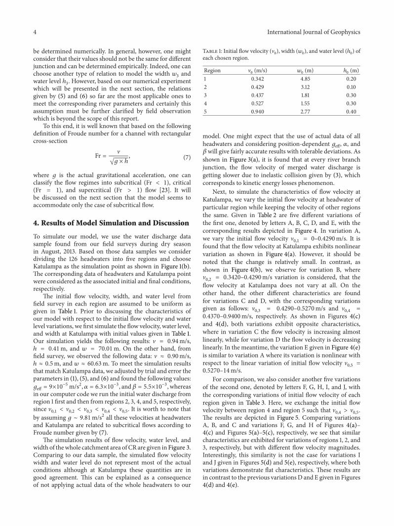
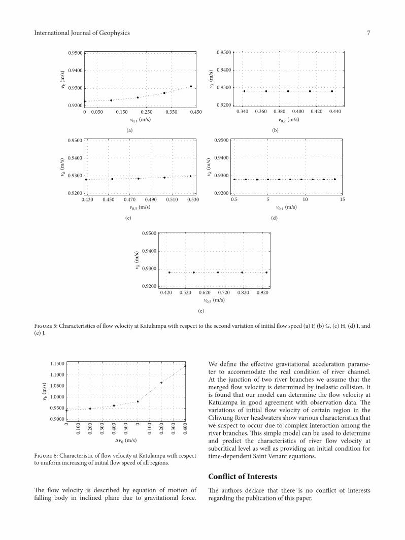
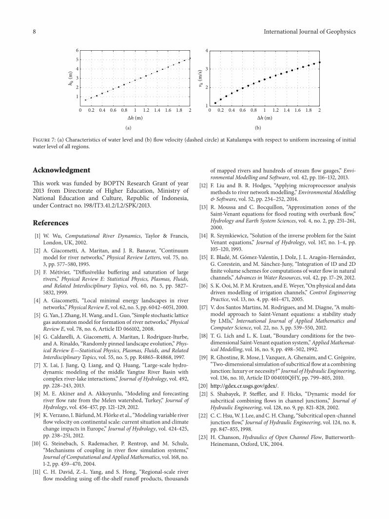