Simulating the Difference between a DES and aSimple Railgun using SPICE

S. HundertmarkFrench-German Research Institute of Saint-Louis, France

Abstract—A DES railgun increases the launch efficency whencompared to a simple railgun setup. In a NGSPICE-Simulationa DES and a simple railgun setup connected to an existing10-MJ capacitor based power supply are compared. Importantparameters like velocity, power and efficiency are used to quantifythe performance gain, when using the mechanically more complexDES setup. The results of this study were used to select the simplerailgun setup as the design for a new barrel to the 10-MJ powersupply.

I. INTRODUCTION

The French-German Research Institute of Saint-Louis (ISL)has an extensive experimental railgun research program. ThePEGASUS railgun installation consists out of a 10 MJ capac-itor based power supply and a 6 m long distributed energysupply (DES) railgun barrel. One focus of research with thisinstallation is the application of different armature conceptsto improve the armature/rail contact behavior [1]. A possible,military application for powerful railguns is as artillery system.The availability of a sufficient amount of electrical poweron modern ships makes the installation of electric guns onthese ships an attractive possibility [2]. A military, fieldablegun system has to be as simple and robust as possible.For a DES barrel, as currently being used in the PEGASUSinstallation, current has to be routed to current injection pointsbeing distributed along the barrel. This makes these barrelsmechanically complex and adds more weight to the front part,increasing the time needed for pointing movements. On theother hand, these barrels are more efficient than comparablesimple railgun barrels. In this paper a simple railgun iscompared to the DES railgun in order to be able to asseshow much better the DES railgun performs. For this a setupclosely resembling the current PEGASUS barrel was comparedto a simple railgun of the same size and connected to thesame power supply. The outcome of this study is used as aguide when deciding on the architecture of a new barrel forthe PEGASUS installation.

II. SIMPLE AND DES RAILGUN

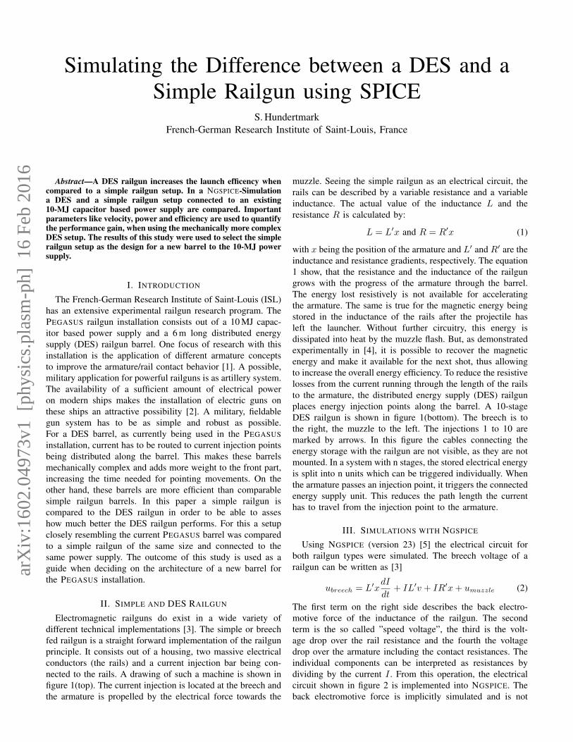
Electromagnetic railguns do exist in a wide variety ofdifferent technical implementations [3]. The simple or breechfed railgun is a straight forward implementation of the railgunprinciple. It consists out of a housing, two massive electricalconductors (the rails) and a current injection bar being con-nected to the rails. A drawing of such a machine is shown infigure 1(top). The current injection is located at the breech andthe armature is propelled by the electrical force towards the

muzzle. Seeing the simple railgun as an electrical circuit, therails can be described by a variable resistance and a variableinductance. The actual value of the inductance L and theresistance R is calculated by:

L = L′x and R = R′x (1)

with x being the position of the armature and L′ and R′ are theinductance and resistance gradients, respectively. The equation1 show, that the resistance and the inductance of the railgungrows with the progress of the armature through the barrel.The energy lost resistively is not available for acceleratingthe armature. The same is true for the magnetic energy beingstored in the inductance of the rails after the projectile hasleft the launcher. Without further circuitry, this energy isdissipated into heat by the muzzle flash. But, as demonstratedexperimentally in [4], it is possible to recover the magneticenergy and make it available for the next shot, thus allowingto increase the overall energy efficiency. To reduce the resistivelosses from the current running through the length of the railsto the armature, the distributed energy supply (DES) railgunplaces energy injection points along the barrel. A 10-stageDES railgun is shown in figure 1(bottom). The breech is tothe right, the muzzle to the left. The injections 1 to 10 aremarked by arrows. In this figure the cables connecting theenergy storage with the railgun are not visible, as they are notmounted. In a system with n stages, the stored electrical energyis split into n units which can be triggered individually. Whenthe armature passes an injection point, it triggers the connectedenergy supply unit. This reduces the path length the currenthas to travel from the injection point to the armature.

III. SIMULATIONS WITH NGSPICE

Using NGSPICE (version 23) [5] the electrical circuit forboth railgun types were simulated. The breech voltage of arailgun can be written as [3]

ubreech = L′xdI

dt+ IL′v + IR′x+ umuzzle (2)

The first term on the right side describes the back electro-motive force of the inductance of the railgun. The secondterm is the so called ”speed voltage”, the third is the volt-age drop over the rail resistance and the fourth the voltagedrop over the armature including the contact resistances. Theindividual components can be interpreted as resistances bydividing by the current I . From this operation, the electricalcircuit shown in figure 2 is implemented into NGSPICE. Theback electromotive force is implicitly simulated and is not

arX

iv:1

602.

0497

3v1

[ph

ysic

s.pl

asm

-ph]

16

Feb

2016

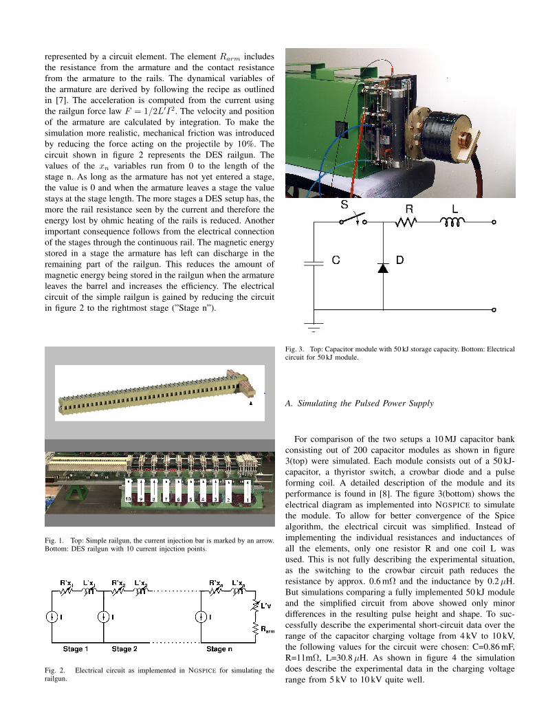
represented by a circuit element. The element Rarm includesthe resistance from the armature and the contact resistancefrom the armature to the rails. The dynamical variables ofthe armature are derived by following the recipe as outlinedin [7]. The acceleration is computed from the current usingthe railgun force law F = 1/2L′I2. The velocity and positionof the armature are calculated by integration. To make thesimulation more realistic, mechanical friction was introducedby reducing the force acting on the projectile by 10%. Thecircuit shown in figure 2 represents the DES railgun. Thevalues of the xn variables run from 0 to the length of thestage n. As long as the armature has not yet entered a stage,the value is 0 and when the armature leaves a stage the valuestays at the stage length. The more stages a DES setup has, themore the rail resistance seen by the current and therefore theenergy lost by ohmic heating of the rails is reduced. Anotherimportant consequence follows from the electrical connectionof the stages through the continuous rail. The magnetic energystored in a stage the armature has left can discharge in theremaining part of the railgun. This reduces the amount ofmagnetic energy being stored in the railgun when the armatureleaves the barrel and increases the efficiency. The electricalcircuit of the simple railgun is gained by reducing the circuitin figure 2 to the rightmost stage (”Stage n”).

Fig. 1. Top: Simple railgun, the current injection bar is marked by an arrow.Bottom: DES railgun with 10 current injection points.

Fig. 2. Electrical circuit as implemented in NGSPICE for simulating therailgun.

Fig. 3. Top: Capacitor module with 50 kJ storage capacity. Bottom: Electricalcircuit for 50 kJ module.

A. Simulating the Pulsed Power Supply

For comparison of the two setups a 10 MJ capacitor bankconsisting out of 200 capacitor modules as shown in figure3(top) were simulated. Each module consists out of a 50 kJ-capacitor, a thyristor switch, a crowbar diode and a pulseforming coil. A detailed description of the module and itsperformance is found in [8]. The figure 3(bottom) shows theelectrical diagram as implemented into NGSPICE to simulatethe module. To allow for better convergence of the Spicealgorithm, the electrical circuit was simplified. Instead ofimplementing the individual resistances and inductances ofall the elements, only one resistor R and one coil L wasused. This is not fully describing the experimental situation,as the switching to the crowbar circuit path reduces theresistance by approx. 0.6 mΩ and the inductance by 0.2µH.But simulations comparing a fully implemented 50 kJ moduleand the simplified circuit from above showed only minordifferences in the resulting pulse height and shape. To suc-cessfully describe the experimental short-circuit data over therange of the capacitor charging voltage from 4 kV to 10 kV,the following values for the circuit were chosen: C=0.86 mF,R=11mΩ, L=30.8µH. As shown in figure 4 the simulationdoes describe the experimental data in the charging voltagerange from 5 kV to 10 kV quite well.

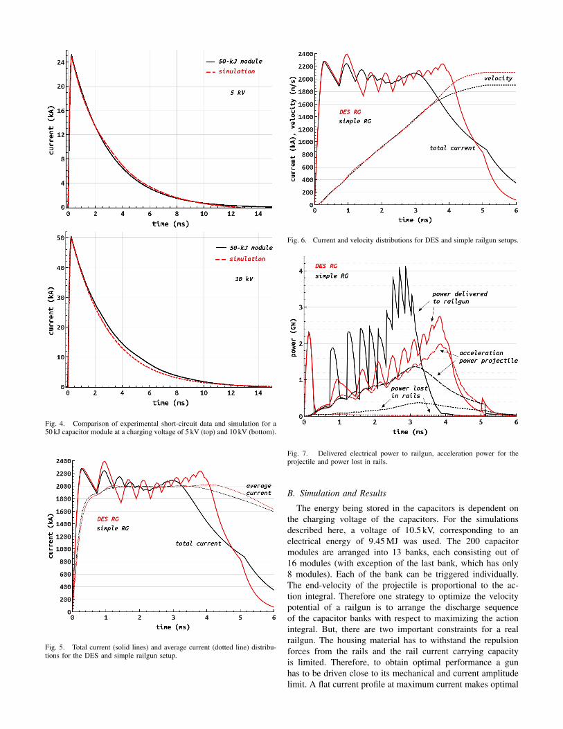
Fig. 4. Comparison of experimental short-circuit data and simulation for a50 kJ capacitor module at a charging voltage of 5 kV (top) and 10 kV (bottom).

Fig. 5. Total current (solid lines) and average current (dotted line) distribu-tions for the DES and simple railgun setup.

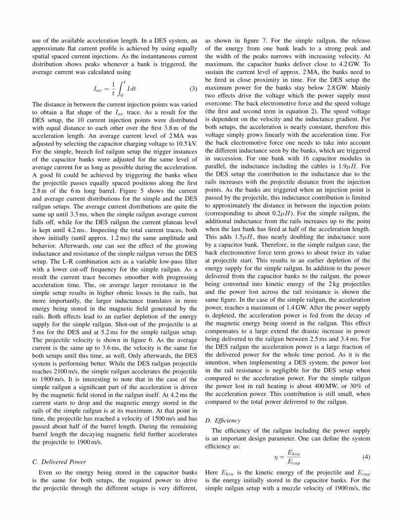
Fig. 6. Current and velocity distributions for DES and simple railgun setups.

Fig. 7. Delivered electrical power to railgun, acceleration power for theprojectile and power lost in rails.

B. Simulation and Results

The energy being stored in the capacitors is dependent onthe charging voltage of the capacitors. For the simulationsdescribed here, a voltage of 10.5 kV, corresponding to anelectrical energy of 9.45 MJ was used. The 200 capacitormodules are arranged into 13 banks, each consisting out of16 modules (with exception of the last bank, which has only8 modules). Each of the bank can be triggered individually.The end-velocity of the projectile is proportional to the ac-tion integral. Therefore one strategy to optimize the velocitypotential of a railgun is to arrange the discharge sequenceof the capacitor banks with respect to maximizing the actionintegral. But, there are two important constraints for a realrailgun. The housing material has to withstand the repulsionforces from the rails and the rail current carrying capacityis limited. Therefore, to obtain optimal performance a gunhas to be driven close to its mechanical and current amplitudelimit. A flat current profile at maximum current makes optimal

use of the available acceleration length. In a DES system, anapproximate flat current profile is achieved by using equallyspatial spaced current injections. As the instantaneous currentdistribution shows peaks whenever a bank is triggered, theaverage current was calculated using

Iav =1

t

∫ t

0

Idt (3)

The distance in between the current injection points was variedto obtain a flat shape of the Iav trace. As a result for theDES setup, the 10 current injection points were distributedwith equal distance to each other over the first 3.8 m of theacceleration length. An average current level of 2 MA wasadjusted by selecting the capacitor charging voltage to 10.5 kV.For the simple, breech fed railgun setup the trigger instancesof the capacitor banks were adjusted for the same level ofaverage current for as long as possible during the acceleration.A good fit could be achieved by triggering the banks whenthe projectile passes equally spaced positions along the first2.8 m of the 6 m long barrel. Figure 5 shows the currentand average current distributions for the simple and the DESrailgun setups. The average current distributions are quite thesame up until 3.3 ms, when the simple railgun average currentfalls off, while for the DES railgun the current plateau levelis kept until 4.2 ms.. Inspecting the total current traces, bothshow initially (until approx. 1.2 ms) the same amplitude andbehavior. Afterwards, one can see the effect of the growinginductance and resistance of the simple railgun versus the DESsetup. The L-R combination acts as a variable low-pass filterwith a lower cut-off frequency for the simple railgun. As aresult the current trace becomes smoother with progressingacceleration time. The, on average larger resistance in thesimple setup results in higher ohmic losses in the rails, butmore importantly, the larger inductance translates in moreenergy being stored in the magnetic field generated by therails. Both effects lead to an earlier depletion of the energysupply for the simple railgun. Shot-out of the projectile is at5 ms for the DES and at 5.2 ms for the simple railgun setup.The projectile velocity is shown in figure 6. As the averagecurrent is the same up to 3.6 ms, the velocity is the same forboth setups until this time, as well. Only afterwards, the DESsystem is performing better. While the DES railgun projectilereaches 2100 m/s, the simple railgun accelerates the projectileto 1900 m/s. It is interesting to note that in the case of thesimple railgun a significant part of the acceleration is drivenby the magnetic field stored in the railgun itself. At 4.2 ms thecurrent starts to drop and the magnetic energy stored in therails of the simple railgun is at its maximum. At that point intime, the projectile has reached a velocity of 1500 m/s and haspassed about half of the barrel length. During the remainingbarrel length the decaying magnetic field further acceleratesthe projectile to 1900 m/s.

C. Delivered Power

Even so the energy being stored in the capacitor banksis the same for both setups, the required power to drivethe projectile through the different setups is very different,

as shown in figure 7. For the simple railgun, the releaseof the energy from one bank leads to a strong peak andthe width of the peaks narrows with increasing velocity. Atmaximum, the capacitor banks deliver close to 4.2 GW. Tosustain the current level of approx. 2 MA, the banks need tobe fired in close proximity in time. For the DES setup themaximum power for the banks stay below 2.8 GW. Mainlytwo effects drive the voltage which the power supply mustovercome: The back electromotive force and the speed voltage(the first and second term in equation 2). The speed voltageis dependent on the velocity and the inductance gradient. Forboth setups, the acceleration is nearly constant, therefore thisvoltage simply grows linearly with the acceleration time. Forthe back electromotive force one needs to take into accountthe different inductance seen by the banks, which are triggeredin succession. For one bank with 16 capacitor modules inparallel, the inductance including the cables is 1.9µH . Forthe DES setup the contribution to the inductance due to therails increases with the projectile distance from the injectionpoints. As the banks are triggered when an injection point ispassed by the projectile, this inductance contribution is limitedto approximately the distance in between the injection points(corresponding to about 0.2µH). For the simple railgun, theadditional inductance from the rails increases up to the pointwhen the last bank has fired at half of the acceleration length.This adds 1.5µH , thus nearly doubling the inductance seenby a capacitor bank. Therefore, in the simple railgun case, theback electromotive force term grows to about twice its valueat projectile start. This results in an earlier depletion of theenergy supply for the simple railgun. In addition to the powerdelivered from the capacitor banks to the railgun, the powerbeing converted into kinetic energy of the 2 kg projectilesand the power lost across the rail resistance is shown thesame figure. In the case of the simple railgun, the accelerationpower, reaches a maximum of 1.4 GW. After the power supplyis depleted, the acceleration power is fed from the decay ofthe magnetic energy being stored in the railgun. This effectcompensates to a large extend the drastic increase in powerbeing delivered to the railgun between 2.5 ms and 3.4 ms. Forthe DES railgun the acceleration power is a large fraction ofthe delivered power for the whole time period. As it is theintention, when implementing a DES system, the power lostin the rail resistance is negligible for the DES setup whencompared to the acceleration power. For the simple railgunthe power lost in rail heating is about 400 MW, or 30% ofthe acceleration power. This contribution is still small, whencompared to the total power delivered to the railgun.

D. Efficiency

The efficiency of the railgun including the power supplyis an important design parameter. One can define the systemefficiency as:

η =Ekin

Ecap(4)

Here Ekin is the kinetic energy of the projectile and Ecap

is the energy initially stored in the capacitor banks. For thesimple railgun setup with a muzzle velocity of 1900 m/s, the

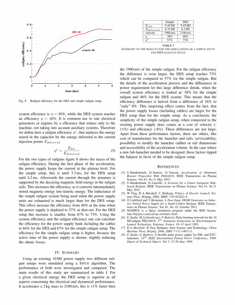
Fig. 8. Railgun efficiency for the DES and simple railgun setup.

system efficiency is η = 38%, while the DES system reachesan efficiency η = 46%. It is common use to rate electricalgenerators or engines by a efficiency that relates only to themachine, not taking into account auxiliary systems. Thereforewe define here a railgun efficiency η?, that replaces the energystored in the capacitor by the energy delivered to the currentinjection points Edelivered

η? =Ekin

Edelivered(5)

For the two types of railguns figure 8 shows the traces of therailgun efficiency. During the first phase of the acceleration,the power supply keeps the current at the plateau level. Forthe simple setup, this is until 3.3 ms, for the DES setupuntil 4.2 ms. Afterwards the current through the armature issupported by the decaying magnetic field energy in the railgunrails. This increases the efficiency, as it converts intermediatelystored magnetic energy into kinetic energy. The inductance ofthe simple railgun system being used when the power supplyunits are exhausted is much larger than for the DES setup.This effect increase the efficiency from 40% at the time whenthe power supply is depleted to 57% at shot-out. For the DESsetup this increase is smaller, from 67% to 73%. Using thesystem efficiency and the railgun efficiency one can calculatethe efficiency for the power supply bank including the cablesto 64% for the DES and 67% for the simple railgun setup. Theefficiency for the simple railgun setup is higher, because theactive time of the power supply is shorter, slightly reducingthe ohmic losses.

IV. SUMMARY

Using an existing 10 MJ power supply two different rail-gun setups were simulated using a SPICE algorithm. Theperformance of both were investigated and compared. Themain results of this study are summarized in table I. Fora given electrical energy the DES setup is superior in allaspects concerning the electrical and dynamical performance.It accelerates a 2 kg mass to 2100 m/s, this is 11% faster then

Simple DESEcap 9.45 MJ 9.45 MJEdelivered 6.33 MJ 6.1 MJvelocity 1900 m/s 2100 m/sη 38% 46%η? 57% 73%

TABLE ISUMMARY OF THE RESULTS FOR THE SIMULATIONS OF A SIMPLE SETUP

AND DES RAILGUN SETUP.

the 1900 m/s of the simple railgun. For the railgun efficiencythe difference is even larger, the DES setup reaches 73%which can be compared to 57% for the simple railgun. Butthe details of the acceleration process and the differences inpower requirement let this large difference shrink, when theoverall system efficiency is looked at: 38% for the simplerailgun and 46% for the DES system. This means that theefficiency difference is halved from a difference of 16% to”only” 8%. This surprising effect comes from the fact, thatthe power supply losses (including cables) are larger for theDES setup than for the simple setup. As a conclusion, thesimplicity of the simple railgun setup, when connected to theexisting power supply does comes at a cost of velocity (-11%) and efficiency (-8%). These differences are not large.Apart from these performance factors, there are others, likecost of manufacture for the launcher and rails, serviceability,possibility to modify the launcher caliber or rail dimensionsand accessibility of the acceleration volume. In the case wherea new lab-launcher needed to be designed, these factors tippedthe balance in favor of the simple railgun setup.

REFERENCES

[1] S. Hundertmark, D. Simicic, G. Vincent, Acceleration of AluminumBooster Projectiles With PEGASUS, IEEE Transactions on PlasmaScience, Vol. 43, No. 5, May 2015.

[2] S. Hundertmark, D. Lancelle, A Scenario for a Future European Ship-board Railgun, IEEE Transactions on Plasma Science, Vol. 43, No. 5,May 2015.

[3] W. Ying, R. A. Marshall, C. Shukang, Pyhsics of Electric Launch, Sci-ence Press, Beijing, 2004, ISBN 7-03-012821-4.

[4] O. Liebfried and V. Brommer, A Four-Stage XRAM Generator as Induc-tive Pulsed Power Supply for a Small-Caliber Railgun, IEEE Transac-tions on Plasma Science, Vol. 41, No. 10, October 2013.

[5] NGSPICE is a Spice simulation program under the BSD license.http://ngspice.sourceforge.net/index.html.

[6] E. Spahn, M. Lichtenberger, F. Hatterer, Pulse forming network for the 10MJ-railgun PEGASUS, 5th European Symposium on ElectromagneticLaunch Technology, Toulouse, France, 10–13 April 1995.

[7] R. A. Marshall, W. Ying, Railguns: their Science and Technology, ChinaMachine Press, Beijing, 2004, ISBN 7-111-14013-3.

[8] E. Spahn, G. Buderer, A flexible pulse power supply for EM- and ETC-launchers, 12th IEEE International Pulsed Power Conference, 1999.Digest of Technical Papers, Vol. 2, 27-30 June 1999.