Embed Size (px)
Citation preview
Journal of Engineering Research and Studies E-ISSN0976-7916
JERS/Vol.II/ Issue II/April-June,2011/131-142
Research Article
LIQUEFACTION CHARACTERISTICS EVALUATION
THROUGH DIFFERENT STRESS-BASED MODELS: A
COMPARATIVE STUDY P. Raychowdhury
1* and P. K. Basudhar
2
Address for Correspondence
1*Department of Civil Engineering, Indian Institute of Technology, Kanpur 208016, India
2Department of Civil Engineering, Indian Institute of Technology, Kanpur 208016, India
E-mail: [email protected]
ABSTRACT The paper presents a comparative study of the predicted response of a liquefiable saturated sand deposit of Nigata city
under different seismic ground motion using three different stress based analytical models due to Finn et al. (1977),
Liou et al. (1977), and Katsikas and Wylie (1982). The results are also compared with simplified methods that are
adopted in the current design practice. It has been found that the models by Finn et al. (1977) and Katsikas and Wylie
(1982) result in close predictions, whereas the predictions by Liou et al. (1977) are significantly different, particularly
for predicting the rate of partial liquefaction for the chosen soil deposit and earthquake motions.
INTRODUCTION
Liquefaction is an earthquake-induced ground
failure phenomenon observed in saturated loose
sand deposits. Liquefaction involves generation
of excess pore pressure, loss of shear strength
and excessive volume contraction with
associated settlement. Although the simple
methods based on SPT and CPT results are most
commonly used in practice and also
recommended in the design provisions (FEMA-
356 and NEHRP, 2000), nonlinear site response
analysis and dynamic time history analyses are
recommended for design of high risk
infrastructures such as dams and nuclear power
plants. If the sand deposit is densely packed,
repeated shearing causes dilation instead of
contraction, helping the excess pore pressure to
be redistributed. The liquefaction potential of a
soil deposit depends on several factors, such as:
void ratio and relative density of soil, depth of
water table, effective confining stress, and
coefficient of lateral earth pressure, seismic and
geologic history of the site and intensity,
duration and other characteristics of ground
shaking. As such, a proper understanding of their
effects for evaluating the liquefaction
characteristics is essential. Seismic response of
saturated sand deposits and liquefaction
phenomenon has gained significant attention
after 1964 Niigata earthquake. Other significant
earthquakes, such as 1964 Alaska, 1989 Loma-
Prieta, 1995 Kobe and 2001 Bhuj earthquake,
have also demonstrated severe damaging
potential of soil liquefaction on buildings,
bridges, railways, ports and other infrastructures.
A qualitative understanding of the mechanism of
liquefaction of saturated sands subjected to
cyclic loading can be explained by critical void
ratio approach (Castro, 1975). Critical void ratio
is the void ratio of any sand, for which there will
be no volume change during drained shear. A
sand deposit having a void ratio above the
critical value tends to contract during shear, and
develops positive pore pressure under undrained
conditions, and has a potential to experience
liquefaction. Conversely, deposits having an
initial void ratio below critical value tend to
dilate during shear, producing a decrease in pore-
water pressure and a corresponding increase in
effective stress under undrained conditions. Till
date significant analytical, experimental,
numerical and post-earthquake field
investigations have been carried out to
understand the mechanism and predict the
potential of liquefaction and related
consequences.
Analytical models are developed to predict
liquefaction characteristics by Martin et al.
(1975), Liou et al. (1977), Finn et al. (1977),
Katsikas and Wylie (1982), Desai (2000),
Liyanapathirana and Poulos (2002), to name a
few. Some of the analytical models adopted
effective stress-based approach (e.g. Liou et al.
(1977), Finn et al. (1977), Katsikas and Wylie

Journal of Engineering Research and Studies E-ISSN0976-7916
JERS/Vol.II/ Issue II/April-June,2011/131-142
(1982), Liyanapathirana and Poulos (2002)),
while few of them adopted energy-based
approach (e.g. Desai, 2000). Experimental
studies including cyclic triaxial tests, shaking
table tests and centrifuge tests have been
conducted for the last four decades (e.g. Seed
and Lee (1966) Elgamal et al. 1996, Ashford et
al. 2000) to validate the theories and better
understand the mechanism. Simplified methods
to evaluate liquefaction characteristics from SPT
and CPT test results are developed by Seed and
Idriss (1982), Tokimatsu and Seed (1987),
Robertson and Wride (1998), Youd et al. (2001)
and Idriss and Boulanger (2008). Although
simplified total stress-based methods are used in
general practice for the ease of computation to
evaluate the liquefaction potential and associate
settlement, these methods are unable to account
for the progressive stiffness degradation of soil
due to repeated shearing and pore-pressure rise
during an earthquake event. As a result,
nonlinear site response analysis and dynamic
time history analyses are recommended for
design of high risk infrastructures such as dams,
bridges and nuclear power plants (Idriss and
Boulanger, 2008). In this study, three different
analytical models by Finn et al. (1977), Liou et
al. (1977), and Katsikas and Wylie (1982) are
studied to compare the response of saturated
sand deposit under earthquake motions. The
reason behind choosing these models for
comparison study are as follows: (a) these
models are pioneering and fundamental for
theoretical assessment of liquefaction
phenomenon, (b) they can account for nonlinear
stress-strain behavior of soil, (c) progressive rise
in excess pore pressure and associated
degradation of soil strength with time are well
captured in these models, and (d) these models
are widely used in the current design practice.
Moreover, a number of new numerical
liquefaction models have been derived based on
these models. For example, the model developed
by Finn et al. (1977), alternatively known as
DESRA model, has been widely used for
nonlinear site response analysis and liquefaction
characterization. Later on, this model is modified
and implemented in widely used software FLAC
(Itasca, 2005) and has been validated against
other software such as SHAKE (Schnabel et al.,
1972). In this study, for the purpose of
comparison, a liquefiable saturated sand deposit
of Niigata city is considered. A nonlinear shear
stress-strain relationship and a gradual
degradation of the shear modulus are considered
for all three models. Cyclic stress ratio, excess
pore pressure generation, effective stress
reduction and development of shear strain are
considered as four most important parameters
characterizing liquefaction potential. Dynamic
time history analysis is carried out to obtain the
time history of the above-mentioned liquefaction
parameters for earthquake motions from the
1964 Niigata and 1995 Kobe earthquakes.
Finally, the responses from these models are
compared with recent simplified methods
summarized in Youd et al. (2001).
Adopted Numerical Models
For the sake of completeness and proper
appreciation a brief description of the considered
models is provided in this section.
Model#1: Finn, Lee and Martin (1977)
This model includes formulation of constitutive
relations incorporating nonlinear methods to
predict the important features of the dynamic
response of saturated sand deposits that generally
occur when the pore-water pressure rises in the
sand deposit during earthquake shaking. The
model takes into account the important factors
that affect the dynamic response of a sand layer,
such as transient pore pressure rise, soil
damping, hardening, variation of shear modulus
with shear strain and changes in effective mean
normal stress.
The stress-strain behavior of sand in this model
is formulated using hyperbolic relationship
adopted by Hardin and Drnebvich (1972) as
shown in Equations 1 through 3.
γτ
γτ
0
0
0
1m
m
m
G
G
+
= (1)
Journal of Engineering Research and Studies E-ISSN0976-7916
JERS/Vol.II/ Issue II/April-June,2011/131-142
(2)
(3)
where, Gm0 and τm0 are initial maximum shear
modulus and maximum shear stress,
respectively; K0 is coefficient of earth pressure at
rest, e is the void ratio, σv' is vertical effective
stress in pound/sq. ft.; and ε' is the effective
angle of shearing resistance. The maximum shear
modulus and shear stress (Gmn and τmn) at the nth
loading cycle are determined from the initial
peak values using the following expressions:
(4)
(5)
where, σv' is the effective vertical stress at the
beginning of nth loading cycle, σv0
' is the initial
effective vertical stress, ε vd is the accumulated
volumetric strain; and H1, H2, H3, and H4 are
constants, that were determined using
calibrations against experiments carried out in
simple shear apparatus. The volumetric strain,
ε vd is again related to the rate of change in pore
pressure (generation or dissipation) in the
following manner:
(6)
where, u is the pore pressure and Er is the one-
dimensional rebound modulus of sand at an
effective stress of σv'. The steps are repeated for
each cycle of an earthquake event using
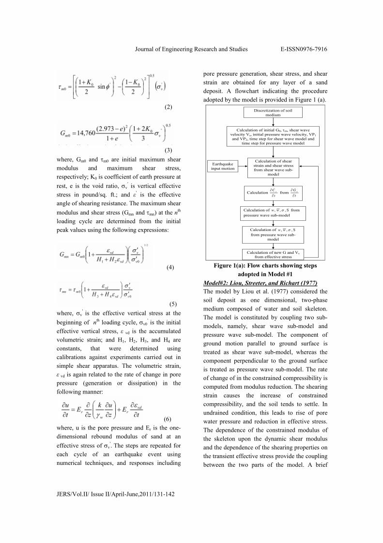
numerical techniques, and responses including
pore pressure generation, shear stress, and shear
strain are obtained for any layer of a sand
deposit. A flowchart indicating the procedure
adopted by the model is provided in Figure 1 (a).
Discretization of soil
medium
Calculation of initial G0, τm, shear wave
velocity Vs, initial pressure wave velocity, VP1
and VP2, time step for shear wave model and
time step for pressure wave model
Calculation of shear
strain and shear stress
from shear wave sub-
model
Earthquake
input motion
Calculation t
C c
∂
∂ from
t
G s
∂
∂
Calculation of S , , , σww
from pressure wave sub-
model
Calculation of S , , , σww from
pressure wave sub-model
Calculation of new G and Vs
from effective stress
Figure 1(a): Flow charts showing steps
adopted in Model #1
Model#2: Liou, Streeter, and Richart (1977)
The model by Liou et al. (1977) considered the
soil deposit as one dimensional, two-phase
medium composed of water and soil skeleton.
The model is constituted by coupling two sub-
models, namely, shear wave sub-model and
pressure wave sub-model. The component of
ground motion parallel to ground surface is
treated as shear wave sub-model, whereas the
component perpendicular to the ground surface
is treated as pressure wave sub-model. The rate
of change of in the constrained compressibility is
computed from modulus reduction. The shearing
strain causes the increase of constrained
compressibility, and the soil tends to settle. In
undrained condition, this leads to rise of pore
water pressure and reduction in effective stress.
The dependence of the constrained modulus of
the skeleton upon the dynamic shear modulus
and the dependence of the shearing properties on
the transient effective stress provide the coupling
between the two parts of the model. A brief
Journal of Engineering Research and Studies E-ISSN0976-7916
JERS/Vol.II/ Issue II/April-June,2011/131-142
discussion on each sub-model and their coupling
is provided herein.
Shear Wave Submodel
The shear wave sub-model is used to calculate
shearing stress, shearing strain, and modulus
reduction caused by the motion bedrock. The
propagation of the shear waves in one-
dimensional unsaturated soil deposits is modeled
by Ramberg-Osgood relationship (Ramberg and
Osgood, 1943) (shown in Equations 7 and 8).
For initial loading:
(7)
For reloading and unloading:
(8)
Where, τi, and γi represent the coordinates of the
strain reversal point on the τ-γ plane. α, R, and
C1 are constants describing a given soil. Gm0 and
τm0 are determined after Hardin and Drnebvich
(1972) as shown in Equations 1 through 3.
The dynamic equation of motion for the shear
wave propagating through the solid matrix of the
soil column in x-direction can be written as:
(9)
And
(10)
where, ρ = mass density of saturated soil, g =
acceleration of gravity, θ = surface slope of the
constant thickness of soil layer, ux = horizontal
particle displacement in x-direction, U = velocity
of the soil skeleton in x-direction.
Pressure Wave Submodel
By assuming the solid grains to be
incompressible and by neglecting small terms,
the relationship can be obtained.
(11)
where, Cw= compressibility of water, P* =
excess pore pressure, n = porosity of soil, w and
w* are displacements defined in such a way, that
volume of solid and volume of water that pass
through a unit area fixed in space are, (1-n)w and
nw*. The quantity –nP
* represents the excess
tensile force acting on the portion of a unit area
of soil occupied by water, is denoted by S*.
(12)
If S0 is initial hydrostatic value of tensile force
and S is the current value of the same quantity,
then,
(13)
Stress-strain relation for the soil skeleton is:
(14)
In the theory of linear poro-elasticity, Cc is
related to G0 and the compressibility of the
skeleton, Cb, by,
(15)
Where, Gs is the secant shear modulus of the soil
skeleton. Finally, propagation of the plane shear
waves in saturated deposits is represented as:
(16)
Coupling Between Two Sub-models
The numerical model for liquefaction is
constituted by coupled shear wave and pressure
wave motions. In the model, the deposit below
water table is divided into a number of equal
distance intervals and both sub-models are
applied to them. Since in saturated soils
volumetric disturbances travel at a speed much
greater than the shear wave speed, N time steps
are needed in the pressure wave sub-model for
every time step in shear wave sub-model.
Journal of Engineering Research and Studies E-ISSN0976-7916
JERS/Vol.II/ Issue II/April-June,2011/131-142
(17)
The shear wave sub-model is first used to
calculate shearing stress, shearing strain, and
reductions in Gs caused by the motion of the
bedrock. The rate of change of in the constrained
compressibility, ∂Cc/∂t is then computed from
∂Gs/∂t. The pressure wave motions generated by
changes in Cc are then calculated from the
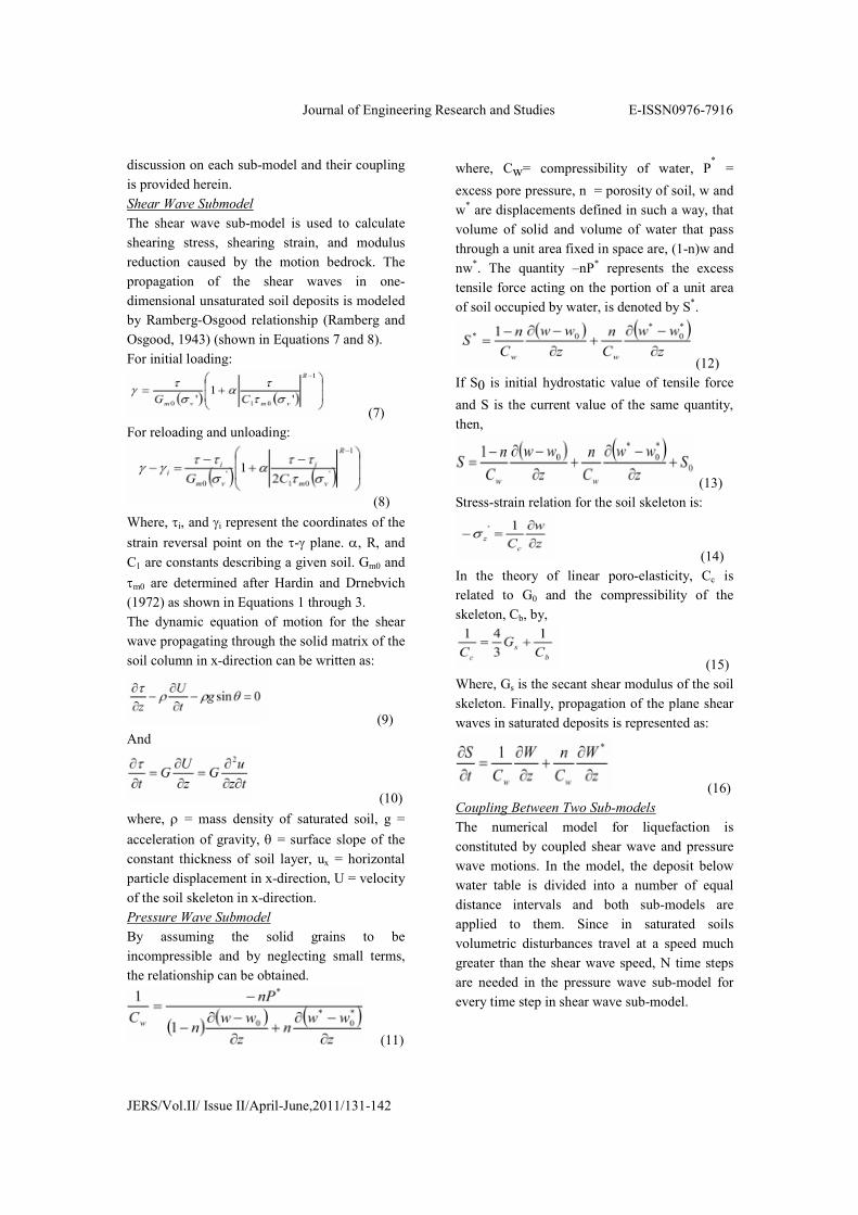
pressure wave sub-model. The shearing strain
causes the increase of Cc, and the soil tends to
settle. In undrained condition, this leads to rise of
pore water pressure and reduction in effective
stress. The steps are summarized in Figure 1 (b).
Calculation of initial G0, τm, shear
wave velocity Vs and time step for
shear wave sub-model
Calculation of shear
strain and shear stress
from shear wave sub-
model
Calculation soil densification
from shear wave sub-model
Calculation of effective stress
from pore water pressure and
total stress
Calculation pore water pressure
and seepage velocity from pressure
wave sub-model
Calculation of new G and Vs
from effective stress
Discretization of soil
medium
Earthquake
input motion
Figure 1(b): Flow charts showing steps
adopted in Model #2
Model#3: Katsikas, and Wylie (1982)
This model is also an effective stress-based
numerical model that provides the interaction
between shearing deformation and transient
pore-water pressure development. One-
dimensional propagation of shear waves through
the solid matrix of the soil and pressure waves
through the pore water is the principal part of the
model. The volumetric soil deformation provides
the means of coupling the shear and pressure
waves during motion.
Specific features of this one-dimensional model
are the preservation of the inelastic soil character
during shearing, coupling between shear wave
propagation and pore-water pressure
development and seepage, and the association of
excess pore-water pressure development with the
inelastic volumetric deformation of the solid
matrix and reasonable validation of the model
against shaking table tests. The modeling
approach is discussed briefly here.
Under cyclic straining the structure change of the
soil is given by,
(18)
where, ∆εv = net solid matrix deformation, ∆εvs
= volume reduction (densification) due to
particle rearrangement, ∆εvr = volume
expansion(rebound) due to relaxation of soil
matrix. Based on a number of experimental
studies, elastic rebound of the soil can be
described as:
(19)
where, εvr is corresponding soil rebound, σ0 is
mean effective stress, and A and σ are constants.
From experimental results an empirical
expression is developed by Katsikas (1979) for
the soil rebound:
(20)
σ0 is mean effective stress in pounds/sq. ft. Then
the soil densification increment, ∆εvs,
corresponding to a time increment ∆t, during
straining may be given as:
(21)
where Nc= Number of cycles from the beginning
of straining, γ(%)= instantaneous shear strain at
the end of a time increment ∆t, ∆γ(%) = change
in shear strain over time ∆t, and A1, A3 =
parameters that depend on soil properties. The
following expressions were derived by the first
Journal of Engineering Research and Studies E-ISSN0976-7916
JERS/Vol.II/ Issue II/April-June,2011/131-142
writer, Christos A. Katsikas, based on the
experimental results:
(22)
(23)
where,Dr= relative density of the soil and D50=
grain diameter in mm corresponding to 50%
finer. The in elastic volumetric deformation of
the solid matrix is associated with the generation
of excess pore water pressure through the
coupling between the shear wave propagation
through soil skeleton and the pressure wave
propagation through pore water. The numerical
analysis is done by method of characteristics.
The steps are shown through a flowchart in
Figure 1(c).
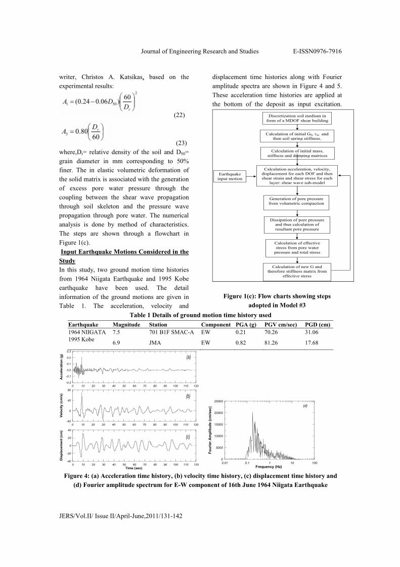
Input Earthquake Motions Considered in the
Study
In this study, two ground motion time histories
from 1964 Niigata Earthquake and 1995 Kobe
earthquake have been used. The detail
information of the ground motions are given in
Table 1. The acceleration, velocity and
displacement time histories along with Fourier
amplitude spectra are shown in Figure 4 and 5.
These acceleration time histories are applied at
the bottom of the deposit as input excitation.
Calculation of initial mass,
stiffness and damping matrices
Discretization soil medium in
form of a MDOF shear building
Calculation of initial G0, τm and
then soil spring stiffness.
Calculation acceleration, velocity,
displacement for each DOF and then
shear strain and shear stress for each
layer: shear wave sub-model
Generation of pore pressure
from volumetric compaction
Calculation of effective
stress from pore water
pressure and total stress
Dissipation of pore pressure
and thus calculation of
resultant pore pressure
Calculation of new G and
therefore stiffness matrix from
effective stress
Earthquake
input motion
Figure 1(c): Flow charts showing steps
adopted in Model #3
Table 1 Details of ground motion time history used
Earthquake Magnitude Station Component PGA (g) PGV cm/sec) PGD (cm)
1964 NIIGATA 7.5 701 B1F SMAC-A EW 0.21 70.26 31.06
1995 Kobe
6.9 JMA EW 0.82 81.26 17.68
0 10 20 30 40 50 60 70 80 90 100 110 120-0.2
-0.1
0.0
0.1
0.2
0.3
Acceleration (g)
0 10 20 30 40 50 60 70 80 90 100 110 120-40
0
40
80
Velocity (cm/s)
(a)
0 10 20 30 40 50 60 70 80 90 100 110 120
Time (sec)
-40
-20
0
20
40
Displacement (cm)
(b)
(c)
0.01 0.1 1 10 100
Frequency (Hz)
0
5000
10000
15000
20000
25000
Fourier Amplitude (cm/sec) (d)
Figure 4: (a) Acceleration time history, (b) velocity time history, (c) displacement time history and
(d) Fourier amplitude spectrum for E-W component of 16th June 1964 Niigata Earthquake
Journal of Engineering Research and Studies E-ISSN0976-7916
JERS/Vol.II/ Issue II/April-June,2011/131-142
0 10 20 30 40 50-1.2
-0.8
-0.4
0.0
0.4
0.8Acceleration (g)
0 10 20 30 40 50
-80
-40
0
40
80
120
Velocity (cm/s)
(a)
0 10 20 30 40 50
Time (sec)
-20
-10
0
10
20
Displacement (cm)
(b)
(c)
0.01 0.1 1 10 100
Frequency (Hz)
0
10000
20000
30000
Fourier Amplitude (cm/sec) (d)
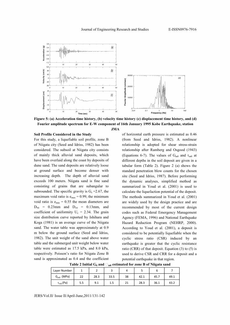
Figure 5: (a) Acceleration time history, (b) velocity time history (c) displacement time history, and (d)
Fourier amplitude spectrum for E-W component of 16th January 1995 Kobe Earthquake, station
JMA
Soil Profile Considered in the Study
For this study, a liquefiable soil profile, zone B
of Niigata city (Seed and Idriss, 1982) has been
considered. The subsoil at Niigata city consists
of mainly thick alluvial sand deposits, which
have been overlaid along the coast by deposits of
dune sand. The sand deposits are relatively loose
at ground surface and become denser with
increasing depth. The depth of alluvial sand
exceeds 100 meters. Niigata sand is fine sand
consisting of grains that are subangular to
subrounded. The specific gravity is Gs =2.67, the
maximum void ratio is emax = 0.99, the minimum
void ratio is emin = 0.55 the mean diameters are
D50 = 0.23mm and D10 = 0.13mm, and
coefficient of uniformity Uc = 2.34. The grain
size distribution curve reported by Ishihara and
Koga (1981) is an average curve of the Niigata
sand. The water table was approximately at 0.9
m below the ground surface (Seed and Idriss,
1982). The unit weight of the sand above water
table and the submerged unit weight below water
table were estimated as 17.5 kPa, and 8.0 kPa,
respectively. Poisson’s ratio for Niigata Zone B
sand is approximated as 0.4 and the coefficient
of horizontal earth pressure is estimated as 0.46
(from Seed and Idriss, 1982). A nonlinear
relationship is adopted for shear stress-strain
relationship after Ramberg and Osgood (1943)
(Equations 6-7). The values of Gm0 and τm0 at
different depths in the soil deposit are given in a
tabular form (Table 2). Figure 2 (a) shows the
standard penetration blow counts for the chosen
site (Seed and Idriss, 1987). Before performing
the dynamic analyses, simplified method as
summarized in Youd et al. (2001) is used to
calculate the liquefaction potential of the deposit.
The methods summarized in Youd et al. (2001)
are widely used by the design practice and are
recommended by most of the current design
codes such as Federal Emergency Management
Agency (FEMA, 1996) and National Earthquake
Hazard Reduction Program (NEHRP, 2000).
According to Youd et al. (2001), a deposit is
considered to be potentially liquefiable when the
cyclic stress ratio (CSR) induced by an
earthquake is greater that the cyclic resistance
ratio (CRR) of that deposit. Equation (3) to (5) is
used to derive CSR and CRR for a deposit and a
potential earthquake in that region.
Table 2 Initial G0 and Am0 estimated for zone B of Niigata sand
Layer Number 1 2 3 4 5 6 7
Gm0 (MPa) 22 28.3 33.5 38 42.1 45.7 49.1
τm0 (Pa) 5.5 9.1 1.5 21 28.3 36.1 43.2
Journal of Engineering Research and Studies E-ISSN0976-7916
JERS/Vol.II/ Issue II/April-June,2011/131-142
0 20 40 60
Blows/ft
80
60
40
20
0
Depth (ft)
20
10
0
Depth (m)
0 0.5 1 1.5 2 2.5
CRR/CSR
80
60
40
20
0
Depth (ft)
20
10
0
Depth (m)
Niigata (M=7.5, pga=0.21g)
Kobe (M=6.9, pga=0.82g)
Liq Non-liq
(a) (b)
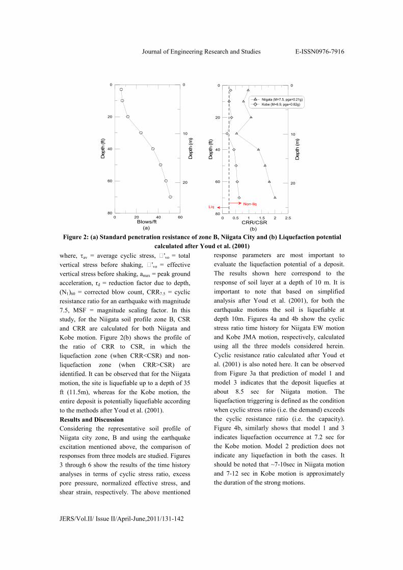
Figure 2: (a) Standard penetration resistance of zone B, Niigata City and (b) Liquefaction potential
calculated after Youd et al. (2001)
where, τav = average cyclic stress, 'vo = total
vertical stress before shaking, 'vo = effective
vertical stress before shaking, amax = peak ground
acceleration, rd = reduction factor due to depth,
(N1)60 = corrected blow count, CRR7.5 = cyclic
resistance ratio for an earthquake with magnitude
7.5, MSF = magnitude scaling factor. In this
study, for the Niigata soil profile zone B, CSR
and CRR are calculated for both Niigata and
Kobe motion. Figure 2(b) shows the profile of
the ratio of CRR to CSR, in which the
liquefaction zone (when CRR<CSR) and non-
liquefaction zone (when CRR>CSR) are
identified. It can be observed that for the Niigata
motion, the site is liquefiable up to a depth of 35
ft (11.5m), whereas for the Kobe motion, the
entire deposit is potentially liquefiable according
to the methods after Youd et al. (2001).
Results and Discussion
Considering the representative soil profile of
Niigata city zone, B and using the earthquake
excitation mentioned above, the comparison of
responses from three models are studied. Figures
3 through 6 show the results of the time history
analyses in terms of cyclic stress ratio, excess
pore pressure, normalized effective stress, and
shear strain, respectively. The above mentioned
response parameters are most important to
evaluate the liquefaction potential of a deposit.
The results shown here correspond to the
response of soil layer at a depth of 10 m. It is
important to note that based on simplified
analysis after Youd et al. (2001), for both the
earthquake motions the soil is liquefiable at
depth 10m. Figures 4a and 4b show the cyclic
stress ratio time history for Niigata EW motion
and Kobe JMA motion, respectively, calculated
using all the three models considered herein.
Cyclic resistance ratio calculated after Youd et
al. (2001) is also noted here. It can be observed
from Figure 3a that prediction of model 1 and
model 3 indicates that the deposit liquefies at
about 8.5 sec for Niigata motion. The
liquefaction triggering is defined as the condition
when cyclic stress ratio (i.e. the demand) exceeds
the cyclic resistance ratio (i.e. the capacity).
Figure 4b, similarly shows that model 1 and 3
indicates liquefaction occurrence at 7.2 sec for
the Kobe motion. Model 2 prediction does not
indicate any liquefaction in both the cases. It
should be noted that ~7-10sec in Niigata motion
and 7-12 sec in Kobe motion is approximately
the duration of the strong motions.
Journal of Engineering Research and Studies E-ISSN0976-7916
JERS/Vol.II/ Issue II/April-June,2011/131-142
0 4 8 12
Time (sec)
-0.2
0.0
0.2
0.4
0.6
0.8 Model #1
Model #2
Model #3
0 2 4 6 8 10
Time (sec)
-0.2
-0.1
0.0
0.1
0.2
0.3
Cyclic Stress Ratio
CRR (Youd et al., 2001) (a) (b)
CRR (Youd et al., 2001)
Figure 3: Cyclic stress ratio: (a) Niigata motion and (b) Kobe motion
Another important feature of the liquefaction is
the generation of excess pore water pressure and
consequent reduction in effective stress. Figure
4a and 4b show the time histories for excess pore
water pressure normalized by total static vertical
stress predicted through the different models as
adopted. It is observed that for Niigata motion,
all three models predict liquefaction at about 10
sec, considering that liquefaction is defined when
excess pore pressure is 100% of the total stress.
However, it can be seen that the rise of excess
pore pressure with time varies significantly from
model to model. Especially model 2 indicates a
very steep curve compared to other two models.
This variation leads to significant difference in
prediction of partial liquefaction characteristics.
For example, at time = 6sec, excess pore
pressure ratio is 22%, 90% and 30% using model
1, 2 and 3, respectively. For Kobe motion,
similar responses are observed. Note that
simplified methods summarized by Youd et al.
(2001) based on SPT and CPT data are unable to
predict the pore-water pressure built up. The
effective stress responses also show the similar
result (Figure 5a and 5b).
Shear strain induced by liquefaction is one of the
most critical consequences of liquefaction.
Liquefaction is often defined as a situation when
shear strain is increased to ±5% (Seed and Idriss,
1987). Figure 6a and 6b show the comparative
predictions of liquefaction induced shear strain
for Niigata and Kobe motions, respectively.
0 4 8 12
Time (sec)
0
20
40
60
80
100 Model #1
Model #2
Model #3
0 4 8 12
Time (sec)
0
20
40
60
80
100
Excess Pore Pressure (%)
(a) (b)
Figure 4: Excess pore pressure ratio: (a) Niigata motion and (b) Kobe motion

Journal of Engineering Research and Studies E-ISSN0976-7916
JERS/Vol.II/ Issue II/April-June,2011/131-142
0 4 8 12
Time (sec)
0.0
0.2
0.4
0.6
0.8
1.0
0 2 4 6 8 10
Time (sec)
0.0
0.2
0.4
0.6
0.8
1.0
Normalized Effective Stress
Model #1
Model #2
Model #3
(a) (b)
Figure 5: Effective stress ratio: (a) Niigata motion and (b) Kobe motion
It can be seen that model 2 indicates liquefaction
occurrence (shear strain = 5%) at about 9 sec for
Niigata motion, whereas other two models
indicates shear strain well below 5% for this
motion. On the other hand, for Kobe motion,
according to model 2, liquefaction occurs (shear
strain = -5%) at 9.5 sec, whereas model 3
indicates liquefaction occurrence at 11 sec.
Model 1 shows that shear strain does not reach
5% for this case. Note that the simplified method
suggested by Tokimatsu and Seed (1987) which
is also adopted in the design practice such as
FEMA-356 (FEMA, 2000) and NEHRP
(NEHRP, 2000), indicates, indicate that the shear
strain of this layer does not reach 5% shear strain
under these earthquake motions. The overall
observation from the comparative study indicates
that model 1 and 3 predictions are similar and are
close to that by simplified methods summarized
in Youd et al. (2001), whereas model 2
prediction is significantly different from that by
the other two models. Since model 1 (Finn et al,
1977, alternatively known as DESRA model) is
widely accepted in the earthquake engineering
community and is well-validated against several
case studies and other dynamic response
evaluation software such as SHAKE (Schnabel
et al., 1972), it may be assumed that this model’s
prediction is somewhat accurate. Based on the
above assumption, it may be concluded that
model 2 is under-predicting the cyclic stress
ratio, but over-predicting the rate of excess pore
pressure generation and the rate of effective
stress reduction significantly. In addition, model
2 is also over-predicting the induced shear strain
in the soil deposit. This over-prediction is
significantly high after 7 sec for Niigata motion
and 9.5 sec for the Kobe motion.
0 4 8 12
Time (sec)
-8
-4
0
4
8
0 2 4 6 8 10
Time (sec)
-2
0
2
4
6
Shear Strain (%)
Model #1
Model #2
Model #3
5% shear strain
Figure 6: Shear strain: (a) Niigata motion and (b) Kobe motion
Journal of Engineering Research and Studies E-ISSN0976-7916
JERS/Vol.II/ Issue II/April-June,2011/131-142
CONCLUSIONS
In this study, a comparative analysis involving
three effective stress-based analytical models,
Finn et al. (1977), Liou et al. (1977) and
Katsikas et al. (1982) is carried out for predicting
the response of a liquefiable saturated sand
deposit of Niigata city under different earthquake
ground motions. All three models assume
nonlinear shear stress-strain relationship, and a
gradual degradation of the shear modulus. The
strength degradation is coupled with pressure
wave propagation through the pore water and
consequent volume change. Comparison results
are shown in terms of four most important
parameters characterizing liquefaction potential:
cyclic stress ratio, excess pore pressure
generation, effective stress reduction and
development of shear strain. Dynamic time
history analysis is carried out to obtain the time
history of the above-mentioned parameters for
earthquake motions from the 1964 Niigata and
1995 Kobe earthquakes. The results are also
compared with simplified methods that are
adopted in current design provisions such as
FEMA (1996) and NEHRP (2000). It has been
found that the prediction by the models of Finn
et al. (1977) and Katsikas et al. (1982) matches
well, whereas the prediction by Liou et al. (1977)
is significantly different for the chosen soil
deposit and ground motions. This difference of
response involving Liou’s model is particularly
significant for the excess pore pressure
generation and consequent strength loss as
indicated by higher rate of partial liquefaction
(Figure 4a-b and 5a-b). This may be due to the
difference in considering the excess pore
pressure generation used in Liou’s model. In
general, however, the time indicating full
liquefaction (pore pressure =100%) is close for
all three models (~10-12 sec).
REFERENCES
• Ashford S. A., Rollins, K. M., and Lane, D.
(2004). “Blast-Induced Liquefaction for Full
Scale Foundation Testing,” Journal of
Geotechnical and Geoenvironmental
Engineering, ASCE, 130(8), 798-806.
• Castro, G. (1975). “Liquefaction and Cyclic
Mobility of Saturated Sand”, Journal of
Geotechnical Engineering Division, ASCE,
101 (6), 551-569.
• Desai, C. (2000). “Evaluation of liquefaction
using disturbed state and energy
Approaches”. Journal of Geotechnical
Engineering Division, ASCE, 126(7), 618–
31.
• Elgamal A. W, Zeghal M, Parra E. (1996)
“Liquefaction of reclaimed island in Kobe,
Japan.” Journal of Geotechnical
Engineering Division, ASCE, 122(1), 39–49.
• FEMA 356, Prestandard and Commentary
for the Seismic Rehabilitation of Buildings,
American Society of Engineers, Virginia.,
2000.
• Finn, W. D. L., Lee, K. W., Martin, G. R.
(1977) “An effective stress model for
liquefaction”. Journal of Geotechnical
Engineering Division, ASCE, 103(GT6),
517–33.
• Itasca (2005). “Fast Lagrangian Analysis of
Continua”. Itasca. FLAC manual, 2005.
• Idriss, I. M. and Boulanger, R. W. (2008).
“Soil Liquefaction during Earthquakes”,
Engineering Monograph, Earthquake
Engineering and Research Institute (EERI),
Oakland, California.
• Ishihara, K. and Koga, Y. (1981). "Case
Studies of Liquefaction in the 1964 Niigata
Earthquake," Soils and Foundations,
Japanese Society of Soil Mechanics and
Foundation Engineering, 21(3), Sept 1981,
35-52.
• Katsikas, C. A. and Wylie, E. B. (1982).
“Sand Liquefaction: Inelastic Effective
Stress Model”. Journal of the Geotechnical
Engineering Division, ASCE, 108(1), 63-81.
• Liou, C. P., Richart, F. E. and Streeter, V. L.
(1977). “Numerical Model for
Liquefaction”. Journal of the Geotechnical
Engineering Division, ASCE, 103 (6), 589-
606.
• Liyanapathirana, D. S. and Poulos, H. G.
(2002). “A numerical model for dynamic
soil liquefaction analysis”. Soil Dynamics
and Earthquake Engineering, 22 (2002),
1007–1015.
• Martin, G. R., Finn, W. D. L. and Seed, H.
B. (1975). “Fundamentals of Liquefaction
under Cyclic Loading”. Journal of the
Geotechnical Engineering Division, ASCE,
101 (5), 423–438.
• NEHRP, Recommended Provisions for
Seismic Regulations for New Buildings,
Building Seismic Safety Council,
Washington, D.C., 2000.
• Ramberg, W. and Osgood, W. T. (1943).
“Description of Stress-strain Curves by
Three Parameters”, Technical Notes 902,
NASA, Washington D. C.

Journal of Engineering Research and Studies E-ISSN0976-7916
JERS/Vol.II/ Issue II/April-June,2011/131-142
• Robertson, P. K., and Wride, C. E. (1998).
‘‘Evaluating cyclic liquefaction potential
using the cone penetration test.’’ Canadian
Geotechnical Journal, 35(3), 442–459.
• Schnabel, P. B., Lysmer, J. and Seed, H. B.
(1972). “SHAKE: A Computer Program for
Earthquake Response Analysis of
Horizontally Layered Sites’, Report No.
EERC 72-12, Earthquake Engineering
Research Center, University of California,
Berkeley.
• Seed, H. B. and Idriss, I. M. (1982). “Soil
Liquefaction during Earthquakes”,
Engineering Monograph, Earthquake
Engineering and Research Institute (EERI),
Oakland, California.
• Seed, H. B. and Lee, K. L. (1966).
“Liquefaction of Saturated Sands During
Cyclic Loading”, Journal of Geotechnical
Engineering Division, ASCE, 92 (SM6),
105-134.
• Tokimatsu, K. and Seed, H. B. (1987).
“Evaluation of Settlement in Sand due to
Earthquake Shaking”. Journal of the
Geotechnical Engineering Division, ASCE,
113 (8), 861-878.
• Youd, T. L. et al. (2001). “Liquefaction
resistance of soils: Summary report from the
1996 NCEER and 1998 NCEER/NSF
Workshops on Evaluation of Liquefaction
Resistance of Soils.” Journal of
Geotechnical and Geoenvironmental
Engineering, ASCE, 127(10), 817–833.


![abueng24i[1] - Technical Journals Online II/JERS VOL II ISSUE IV... · of the system ISI on the signal. This set of decision variables can be defined in terms of their respective](https://img.pdfslide.us/doc/110x75/5c97b14409d3f20d198c93bf/abueng24i1-technical-journals-iijers-vol-ii-issue-iv-of-the-system-isi.jpg)