Research Article Calculation of Weighted Geometric ...downloads.hindawi.com/journals/jam/2013/953048.pdf · Research Article Calculation of Weighted Geometric Dilution of Precision

Hindawi Publishing CorporationJournal of Applied MathematicsVolume 2013, Article ID 953048, 10 pageshttp://dx.doi.org/10.1155/2013/953048

Research ArticleCalculation of Weighted Geometric Dilution of Precision

Chien-Sheng Chen,1 Yi-Jen Chiu,2 Chin-Tan Lee,3 and Jium-Ming Lin4

1 Department of Information Management, Tainan University of Technology, Tainan, Taiwan2Department of Digital Entertainment and Game Design, Taiwan Shoufu University, Tainan, Taiwan3Department of Electronic Engineering, National Quemoy University, Kinmen, Taiwan4Department of Communication Engineering, Chung-Hua University, Hsinchu, Taiwan

Correspondence should be addressed to Chien-Sheng Chen; [email protected]

Received 20 April 2013; Revised 28 August 2013; Accepted 3 September 2013

Academic Editor: Anyi Chen

Copyright © 2013 Chien-Sheng Chen et al. This is an open access article distributed under the Creative Commons AttributionLicense, which permits unrestricted use, distribution, and reproduction in any medium, provided the original work is properlycited.

To achieve high accuracy in wireless positioning systems, both accurate measurements and good geometric relationship betweenthe mobile device and the measurement units are required. Geometric dilution of precision (GDOP) is widely used as a criterionfor selecting measurement units, since it represents the geometric effect on the relationship between measurement error andpositioning determination error. In the calculation of GDOP value, the maximum volume method does not necessarily guaranteethe selection of the optimal four measurement units with minimum GDOP.The conventional matrix inversion method for GDOPcalculation demands a large amount of operation and causes high power consumption. To select the subset of the most appropriatelocation measurement units which give the minimum positioning error, we need to consider not only the GDOP effect but also theerror statistics property. In this paper, we employ the weighted GDOP (WGDOP), instead of GDOP, to select measurement units soas to improve the accuracy of location. The handheld global positioning system (GPS) devices and mobile phones with GPS chipscan merely provide limited calculation ability and power capacity. Therefore, it is very imperative to obtain WGDOP accuratelyand efficiently. This paper proposed two formations of WGDOP with less computation when four measurements are available forlocation purposes. The proposed formulae can reduce the computational complexity required for computing the matrix inversion.The simplerWGDOP formulae for both the 2D and the 3D location estimation, without inverting a matrix, can be applied not onlyto GPS but also to wireless sensor networks (WSN) and cellular communication systems. Furthermore, the proposed formulae areable to provide precise solution of WGDOP calculation without incurring any approximation error.

1. Introduction

In positioning the location estimates are determined throughthe received signals transmitted by the mobile devices at a setof base stations (BSs), satellites, or other sensors. First, thelength or direction of the radio path is determined throughsignal measurements. Secondly, the MS position is derivedfrom radio location algorithms and known geometric rela-tionships. Mobile positioning systems have received signifi-cant attention, and various location technologies have beenproposed in the past few years. Among the techniques formobile positioning there are two major categories—handset-based and network-based schemes. Both approaches havetheir advantages and limitations. Global positioning system

(GPS) is a positioning system that can provide position,velocity, and time information to a user. Handset-based solu-tions generally require a handset modification to calculateits own position when they are fully or partially equippedwith a GPS receiver. The advantages of using handset-based methods are that they have global coverage andusually provide much more accurate location measurements.The drawbacks of the handset-based methods include cost,redundant hardware, and economical integrated technology.The reliability of GPS measurements is greatly compromisedin a building or shadowed environments, where direct line-of-sight (LOS) propagation is not available. Without the aidof satellite systems, network-based positioning schemes usetime and angle measurements to determine the MS location

2 Journal of Applied Mathematics

or to assist the process of MS location determination. Insteadof using all seven BSs, four BSs with better geometry are goodenough to provide sufficient measurements for positioningin cellular communication networks. The network-basedlocation schemes are relatively less complex on hardwarewhen compared with the handset-based methods. They canbe employed in many situations where GPS signal cannot,for example, indoor environment and urban canyon areas,or when GPS-embedded handsets are not available. Formany applications in wireless sensor networks (WSN), likeenvironmental sensing and activities measuring, it is crucialto know the locations of the sensor nodes in network-basedpositioning; this is known as a “localization problem” [1]. Anideal location technology should be able to provide a robustestimate of location in all environments.

This paper considers both the network-based methodand the handset-based method, employing the concept ofgeometric dilution of precision (GDOP), which was initiallydeveloped as a criterion for selecting the optimal 3D geo-metric configuration of satellites in GPS. The general objectof the GPS satellite selection algorithm is to minimize theGDOP to improve the position accuracy. The smaller valueof GDOP is calculated, the better geometric configurationwe will have. The redundant measurements will bring largeamount of computation and may not provide significantlyimproved location accuracy. When enough measurementsare available, the optimal measurements selected with theminimum GDOP can prevent the poor geometry effects andhave the potential of obtaining greater location accuracy.

There have been extensive researches trying to obtain anapproximate GDOP value without executing matrix inver-sion in the past few years. Simon and El-Sherief [2, 3] pro-posed the employment of back-propagation neural network(BPNN) [4] to obtain an approximation for the GDOP func-tion.TheBPNN is employed to learn the relationship betweenthe entries of a measurement matrix and the eigenvaluesof its inverse. Three other input-output relationships wereproposed in [5]. We present the resilient back-propagation(Rprop) architectures to obtain the approximate GDOP[6]. The matrix inversion method for GDOP calculationis born with significant computational burden. GDOP isapproximately inversely proportional to the volume of thetetrahedron formed by the tips of four unit vectors directedto the selected satellites in GPS [7]. The four satellites evenlydistribute with the maximum volume which brings the moreaccurate location estimation. The maximum volume methodrequires low computing time in selecting a subset withthe largest tetrahedron as the optimum [8]. However, it isnot suitable to use this method because it may not selectthe desired satellites with the minimum GDOP. The maindisadvantage of these methods is to incur approximationerrors. To avoid these disadvantages, a simple closed-formformula for GDOP calculation is proposed in [9].

Traditionally, the GDOP computation assumes that thepseudorange errors are independent and identical [10].Several methods based on GDOP have been proposed toimprove the GPS positioning accuracy [7, 9, 11]. In fact,measurements usually have different error variances [12].Ranging error of GPS is caused by many sources, such as

the effect of ionosphere delay, tropospheric delay, carrier-to-noise ratio, and multipath. GDOP and the effect of theseerrors can be considered simultaneously; the extension ofGDOP criteria is used for satellite selection in [13]. Thesatellite signal is also approximated by combining the userrange accuracy value, carrier-to-noise ratio, elevation angle,and the date of ephemeris. The weighted GDOP (WGDOP)which takes these errors into account was proposed in [14].The elevation of each satellite and signal-to-noise-ratio (SNR)are introduced as fuzzy subset to weight GDOP and providethe positioning solution [15]. When baro-altitude measure-ments or a priori terrain elevation information is used, theconventional GDOP formula cannot be applied and must bemodified [16] in order to reduce the influence of satelliteswith a large error and evaluates the influence of each satelliteon the arrangement of satellites. The GDOP was focusedas a factor to determine the weight matrix and improveprecision in GPS measurements [17]. The combinations ofthe GPS and Galileo satellite constellations will provide morevisible satellites with better geometric distribution, and theavailability of satellites will be significantly improved. A novelalgorithm, namely, the WGDOP minimum algorithm, wasproposed in [18] for the combined GPS-Galileo navigationreceiver. In addition to the aforementioned, several paperswhich focus on WGDOP concepts have been proposed toimprove the GPS positioning accuracy [19–21]. Taking thedifferent variances of the satellites into account, researchershave proposed various WGDOP measures [13–21]. Much ofthe research literature needs matrix inversion to calculateWGDOP. Though they can guarantee to achieve the optimalsubset, the computational complexity is usually too expensiveto be practical.

High accuracy in wireless positioning system requiresboth the accurate measurement and a good effect of GDOP.When the measurements have different error variances orcome from integrated positioning systems, WGDOP mini-mum criterion is appropriate to select the appropriate mea-surement units to diminish the positioning error.The optimalmeasurements selected with theminimumWGDOP can helpreduce the adverse geometry effects. Increasing the number ofsatellites will always reduce theWGDOP value, since the bestWGDOP can be obtained by computing all satellites in view.If the number of visible satellites is not large, the all-in-viewmethod is a good choice to provide high accuracy positioning[15]. In order to further improve the positioning accuracy,the combined use of multiconstellation can be employed.Therewill be 70∼90 navigation satellites operating at the sametimewhenGlonass andGalileo reach full operation capability[22]. In any moment, there are more than 30 satellites inview in the multiconstellation navigation systems. To employall-in-view method for positioning is very difficult for us inthe future. Due to limited resources associated with manymobile devices and because the number of visible satellites isvery large [18], measurement unit selection techniques can beused. If we select 4 out of 30 satellites, the number of possiblesubset is 27405. The calculation of WGDOP is a time andpower consuming process, and fast calculation of WGDOPis most anticipated.WGDOP is computed for all subsets, and

Journal of Applied Mathematics 3

the subset which gives the smallest WGDOP is selected forlocation estimation.

The growth ofGPS embedded into currentmobile phonescontinues to grow rapidly, as many mobile phones now arealready equipped with GPS inside. Despite their performanceincreases, these devices still possess limited resources, suchas the number of channels, battery capacities, and process-ing capability. Satellite selection can reduce the number ofsatellites used to position and as a result reducing the amountof calculation greatly. The number of measurements can berestricted and the resulting saving in load on the processorcan be used to offer more spare processing time which can beused for other user specific requirements. On the other hand,reducing the signal-processing time of the receiver dedicatedto satellite selection implies both increasing the processingcapabilities available for other purposes and saving battery.The conventional method for calculating WGDOP is to usematrix inversion, which requires enormous amount of com-putation. This can present challenges to real-time practicalapplications. Therefore, it is very critical to select a subsetwith the most appropriate measurement units rapidly andreasonably before positioning.

To calculate WGDOP in the form of 2D and 3D formula-tions effectively, the closed-form solutions for two WGDOPformations are proposed for the case of each measurementwith a unique variance and one of the measurements withhigher location precision. The computation load of the pro-posed formulae is greatly less than that of thematrix inversionmethod. When exactly four measurements are used, theproposed formulae provide the best computational efficiency.The proposed formulae can also provide the exact solution totheWGDOP calculation and do not incur any approximationerrors. The relatively simple closed-form WGDOP formulaecan be implemented in the aforementioned papers [13–21]. The calculations of WGDOP for fast evaluation can beapplied in GPS, WSN, and cellular communication systems.In practice, the measurement units of GPS, WSN, andcellular communication systems are satellites, sensors, andBSs, respectively.

The author of this paper proposed two novel architecturesand presented four original architectures based on Rpropneural network to approximate WGDOP [23]. The disad-vantage of Rprop-based WGDOP algorithm is the need of atraining phase with several input-output patterns. We collectthe elements of relatedmatrix and the desiredWGDOP valueto train the neural network prior to the practicaluse. Afterthe training, the elements of geometry matrix and weightedmatrix as input data can not only pass through the trainedRprop but also predict the better appropriate WGDOP. Fromsimulation results, the proposed WGDOP formulae alwaysprovide much better accuracy than Rprop-based WGDOPapproximation [23]. But the proposed efficient formulae forWGDOP have been developed when there are exactly fourmeasurement units used.

The remainder of this paper is organized as follows:Section 2 describes the concepts of GDOP and WGDOP.Section 3 reviews an efficient solution for the calculation ofGDOP. The closed-form formulae for WGDOP calculationsin the case of four measurements with unequal variances

are proposed in Section 4. In Section 5, we examine theperformance of the proposed formulae through simulationexperiments. Conclusion is given in Section 6.

2. GDOP and WGDOP

GDOP is a task of choosing the appropriate measurementunits, which results in a better geometric configuration anda more accurate position estimate. In order to achieve betterpositioning accuracy, it is desirable to select the combinationofmeasurements with GDOP as small as possible. Using a 3DCartesian coordinate system, the distances between satellite 𝑖and the user can be expressed as

𝑟

𝑖=

√

(𝑥 − 𝑋

𝑖)

2+ (𝑦 − 𝑌

𝑖)

2+ (𝑧 − 𝑍

𝑖)

2+ 𝐶 ⋅ 𝑡

𝑏+ V𝑟𝑖, (1)

where (𝑥, 𝑦, 𝑧) and (𝑋

𝑖, 𝑌

𝑖, 𝑍

𝑖) are the locations of the user

and satellite 𝑖, respectively; 𝐶 is the speed of light, 𝑡𝑏denotes

the time offset, and V𝑟𝑖is pseudorange measurements noise.

Equation (1) is linearized through the use of a Taylor seriesexpansion around the approximate user position (𝑥, 𝑦, ��) andthe first two terms are retained. Defining 𝑟

𝑖as 𝑟𝑖at (𝑥, 𝑦, ��),

we can obtain

Δ𝑟 = 𝑟

𝑖− 𝑟

𝑖≅ 𝑒

𝑖1𝛿

𝑥+ 𝑒

𝑖2𝛿

𝑦+ 𝑒

𝑖3𝛿

𝑧+ 𝐶 ⋅ 𝑡

𝑏+ V𝑟𝑖, (2)

where 𝛿𝑥, 𝛿𝑦, and 𝛿

𝑧are, respectively, coordinate offsets of 𝑥,

𝑦, and 𝑧,

𝑒

𝑖1=

𝑥 − 𝑋

𝑖

𝑟

𝑖

, 𝑒

𝑖2=

𝑦 − 𝑌

𝑖

𝑟

𝑖

, 𝑒

𝑖3=

�� − 𝑍

𝑖

𝑟

𝑖

,

𝑟

𝑖=

√

(𝑥 − 𝑋

𝑖)

2+ (𝑦 − 𝑌

𝑖)

2+ (�� − 𝑍

𝑖)

2.

(3)

(𝑒

𝑖1, 𝑒

𝑖2, 𝑒

𝑖3), 𝑖 = 1, 2, . . . , 𝑛, denote the line-of-sight (LOS)

vector from the satellites to the user.The linearized pseudorange measurement equations take

the form

𝑧 = 𝐻𝛿 + V, (4)

where 𝑧 =

[

[

[

𝑟1−𝑟1

𝑟2−𝑟2

...𝑟𝑛−𝑟𝑛

]

]

]

, 𝛿 = [

𝛿𝑥

𝛿𝑦

𝛿𝑧

𝑐⋅𝑡𝑏

], V =

[

[

V𝑟1

V𝑟2

...V𝑟𝑛

]

]

, and 𝐻 =

[

[

𝑒11𝑒12𝑒131

𝑒21𝑒22𝑒231

......

......

𝑒𝑛1𝑒𝑛2𝑒𝑛31

]

]

is the geometry matrix.

According to the least square algorithm (LS), the solutionto (4) is given by

𝛿 = (𝐻

𝑇𝐻)

−1

𝐻𝑧.(5)

Assume that the pseudorange errors are uncorrelated withequal variances 𝜎

2, the error covariance matrix can beexpressed as

𝐸 [(

𝛿 − 𝛿) (

𝛿 − 𝛿)

𝑇

] = 𝜎

2⋅ (𝐻

𝑇𝐻)

−1

. (6)


The variances are functions of the diagonal elements of(𝐻

𝑇𝐻)

−1.TheGDOP is ameasure of accuracy for positioningsystems and depends solely on the geometry matrix𝐻

GDOP =

√tr (𝐻𝑇𝐻)

−1.

(7)

In fact, each measurement error does not have the samevariance, especially for the combination of different systems.The covariance matrix represents the uncertainty in thepseudorange measurements and has the following form:

𝐸 (VV𝑇) =

[

[

[

[

[

[

𝜎

2

10 0 0 0

0 𝜎

2

20 0 0

0 0 𝜎

2

30 0

0 0 0 d 0

0 0 0 0 𝜎

2

𝑛

]

]

]

]

]

]

. (8)

𝑊 is a diagonal matrix and defined as a weighted matrix

𝑊=

[

[

[

[

[

[

1/𝜎

2

10 0 0 0

0 1/𝜎

2

20 0 0

0 0 1/𝜎

2

30 0

0 0 0 d 0

0 0 0 0 1/𝜎

2

𝑛

]

]

]

]

]

]

=

[

[

[

[

[

[

𝑘

10 0 0 0

0 𝑘

20 0 0

0 0 𝑘

30 0

0 0 0 d 0

0 0 0 0 𝑘

𝑛

]

]

]

]

]

]

,

(9)

where 𝜎2𝑖= 1/𝑘

𝑖, 𝑖 = 1, 2, . . . , 𝑛 are the variances of the meas-

urement errors.With the weighting matrix defined above, the solution to

the weighted least square (WLS) can be expressed as

𝛿 = (𝐻

𝑇𝑊𝐻)

−1

𝐻

𝑇𝑊𝑧.

(10)

Taking into account that all measurement units containdifferent variances, the positioning algorithm using WLSestimation provides higher location accuracy than the LS esti-mation. Having considered both the geometric configurationand the priori knowledge of error models simultaneously,we choose WGDOP, instead of GDOP, for measurementsselection to achieve effective performance improvement.Theoptimal subset is the one with the minimumWGDOP, whichis given by the trace of the inverse of the𝐻𝑇𝑊𝐻matrix

WGDOP =

√tr (𝐻𝑇𝑊𝐻)

−1.

(11)

We can compute the WGDOP value of each subset, andthen the subsets with minimum WGDOP are the selectedmeasurement units. The conventional method for calcu-lating WGDOP is to use matrix inversion for all subsets.The method can guarantee the optimal subset; however, itpresents a heavy computational burden.

3. Calculation of GDOP forFour Measurements

In the time of arrival (TOA) positioning methods, whichis applied to GPS, the TOA circle becomes the sphere inspace and the fourth measurement is required to solve the

receiver-clock bias for a 3D solution. The bias is the clocksynchronization error between the receiver and the satellite.In practice, the time of user is significantly more inaccuratethan that of an atomic clock on the satellite. In order tocorrect the clock bias errors present at the receiver of the usersend, the measurement from the fourth satellite is employed.Getting information from the fourth measurement makesit possible to solve for this fourth unknown. Even thoughthere are more than four satellites in view, a subset with foursatellites is sufficient providing the sufficient measurementsfor navigation solution even though more than four satellitesare in view, which is called the optimum four GPS satellitespositioning [15]. The selection of four visible satellites toprovide the suitable GPS positioning accuracy is presentedin several papers [13–17]. Thus, we propose to take only fourBSs with better geometry out of seven to estimate the MSlocation in cellular communication networks. For practicalreal-time applications, the number of selected measurementunits should not be large. The efficient closed-form solutionwith simpler calculation for a four-satellite case is proposedin [9].

By using of the following properties:

(𝑈𝑉)

−1= 𝑉

−1𝑈

−1,

tr (𝑈𝑉) = tr (𝑉𝑈) ,

(12)

we have tr (𝑈𝑉)

−1= tr (𝑉𝑈)

−1.From (7), the GDOP can be written as

GDOP =

√tr (𝐻𝑇𝐻)

−1=

√tr (𝐻𝐻

𝑇)

−1.

(13)

By defining the variable𝐵

𝑖𝑗= 𝑒

𝑖1𝑒

𝑗1+ 𝑒

𝑖2𝑒

𝑗2+ 𝑒

𝑖3𝑒

𝑗3+ 1, 1 ≤ 𝑖 < 𝑗 ≤ 4, (14)

and using the following relation that

𝑒

2

𝑖1+ 𝑒

2

𝑖2+ 𝑒

2

𝑖3= 1, 𝑖 = 1, 2, 3, 4, (15)

we have

𝐻𝐻

𝑇=

[

[

[

[

2 𝐵

12𝐵

13𝐵

14

𝐵

122 𝐵

23𝐵

24

𝐵

13𝐵

232 𝐵

34

𝐵

14𝐵

24𝐵

342

]

]

]

]

. (16)

Defining the following variables:

𝑎 = (𝐵

12𝐵

34+ 𝐵

13𝐵

24− 𝐵

14𝐵

23)

2− 4𝐵

12𝐵

34𝐵

13𝐵

24,

(17a)

𝑏 = 16 − 4 (𝐵

2

12+ 𝐵

2

13+ 𝐵

2

14+ 𝐵

2

23+ 𝐵

2

24+ 𝐵

2

34) , (17b)

𝑐 = 2 [𝐵

12(𝐵

13𝐵

23+ 𝐵

14𝐵

24) + 𝐵

34(𝐵

13𝐵

14+ 𝐵

23𝐵

24)] ,

(17c)

the GDOP can be written as [9]

GDOP =√

16 + 𝑏 + 𝑐

𝑎 + 𝑏 + 2𝑐

.

(18)

Note that both 𝐵

12𝐵

34and 𝐵

13𝐵

24appear twice in the

expression of 𝑎, and two multiplications can be eliminated.The closed-form equation needs only 39 multiplications, 34additions, 1 division, and 1 square root.


4. Calculation of WGDOP forFour Measurements

To further reduce the computational overhead and improvethe location performance, the selection of the optimal mea-surement units is necessary. Since the statistics of differentlocation measurement units are, in general, not equal to eachother, WGDOP is appropriate to an index for the precisionof location in different networks, such as GPS, WSN, andcellular communication systems.The steps for positioning arelisted as follows.

(1) We will first select four measurements among 𝑛

measurement units to generate the subsets; thus, the 𝑛measurement units are classified into 𝐶(𝑛, 4) possiblesubsets.

(2) WGDOP is computed for all possible subsets of fourmeasurement units.

(3) The subset which gives the smallest WGDOP isselected as the optimal subset.

(4) Finally, the four measurements of this subset can beused to find out the location solution.

The calculation of WGDOP takes considerable computingtime; it is very imperative to accelerate the computationof WGDOP in real-time application. In this paper, wepropose the efficient closed-form solution of two WGDOPformations, which includes the effect of GDOP and errorstatistics properties simultaneously.These solutions, with thesimplified form for WGDOP calculation, can apply to allpossible subsets in 3Dand 2D scenarios and requiremuch lesscomputation compared to the conventional matrix inversionmethod.

4.1. Type 1: FourMeasurements Have Different Error Variances

4.1.1. 3𝐷 Case. From (11) and by using the properties of thebasic algebra theory,WGDOPcan be alternatively recognizedas

WGDOP =

√tr (𝐻𝑇𝑊𝐻)

−1=

√tr (𝐻𝐻

𝑇𝑊)

−1.

(19)

By using (14) and (15), we have

𝐻𝐻

𝑇𝑊 =

[

[

[

[

𝑒

11𝑒

12𝑒

131

𝑒

21𝑒

22𝑒

231

𝑒

31𝑒

32𝑒

331

𝑒

41𝑒

42𝑒

431

]

]

]

]

[

[

[

[

𝑒

11𝑒

21𝑒

31𝑒

41

𝑒

12𝑒

22𝑒

32𝑒

42

𝑒

13𝑒

23𝑒

33𝑒

43

1 1 1 1

]

]

]

]

×

[

[

[

[

𝑘

10 0 0

0 𝑘

20 0

0 0 𝑘

30

0 0 0 𝑘

4

]

]

]

]

,

(20)

thus

𝐻𝐻

𝑇𝑊 =

[

[

[

[

2𝑘

1𝑘

2𝐵

12𝑘

3𝐵

13𝑘

4𝐵

14

𝑘

1𝐵

122𝑘

2𝑘

3𝐵

23𝑘

4𝐵

24

𝑘

1𝐵

13𝑘

2𝐵

232𝑘

3𝑘

4𝐵

34

𝑘

1𝐵

14𝑘

2𝐵

24𝑘

3𝐵

342𝑘

4

]

]

]

]

. (21)

The WGDOP parameter is the square root of the sum ofdiagonal terms of the matrix (𝐻𝐻

𝑇𝑊)

−1

WGDOP

=

√tr (𝐻𝐻

𝑇𝑊)

−1

=√(𝐻𝐻

𝑇𝑊)

−1

1,1+ (𝐻𝐻

𝑇𝑊)

−1

2,2+ (𝐻𝐻

𝑇𝑊)

−1

3,3+ (𝐻𝐻

𝑇𝑊)

−1

4,4.

(22)

(𝐻𝐻

𝑇𝑊)

−1

𝑖,𝑖is defined as the 𝑖th element on the diagonal of

matrix (𝐻𝐻

𝑇𝑊)

−1

tr (𝐻𝐻

𝑇𝑊)

−1

=

4

∑

𝑖=1

(𝐻𝐻

𝑇𝑊)

−1

𝑖,𝑖

=

tr [adj (𝐻𝐻

𝑇𝑊)]

det (𝐻𝐻

𝑇𝑊)

=

4

∑

𝑖=1

cof𝑖,𝑖(𝐻𝐻

𝑇𝑊)

det (𝐻𝐻

𝑇𝑊)

.

(23)

The term adj(𝐻𝐻

𝑇𝑊) is the adjoint of𝐻𝐻

𝑇𝑊 and the cofac-

tor, and cof𝑖,𝑖(𝐻𝐻

𝑇𝑊) is the determinant of the submatrix

of 𝐻𝐻

𝑇𝑊 by deleting the 𝑖th row and the 𝑖th column. The

cofactors can be obtained as

cof1,1

(𝐻𝐻

𝑇𝑊)

= 𝑘

2𝑘

3𝑘

4[8 + 2 (𝐵

23𝐵

24𝐵

34− (𝐵

2

23+ 𝐵

2

24+ 𝐵

2

34))] ,

(24a)

cof2,2

(𝐻𝐻

𝑇𝑊)

= 𝑘

1𝑘

3𝑘

4[8 + 2 (𝐵

13𝐵

14𝐵

34− (𝐵

2

13+ 𝐵

2

14+ 𝐵

2

34))] ,

(24b)

cof3,3

(𝐻𝐻

𝑇𝑊)

= 𝑘

1𝑘

2𝑘

4[8 + 2 (𝐵

12𝐵

14𝐵

24− (𝐵

2

12+ 𝐵

2

14+ 𝐵

2

24))] ,

(24c)

cof4,4

(𝐻𝐻

𝑇𝑊)

= 𝑘

1𝑘

2𝑘

3[8 + 2 (𝐵

12𝐵

13𝐵

23− (𝐵

2

12+ 𝐵

2

13+ 𝐵

2

23))] .

(24d)

After some algebraicmanipulation, the determinant ofmatrix𝐻𝐻

𝑇𝑊 can be written as

det (𝐻𝐻

𝑇𝑊) = 𝑘

1𝑘

2𝑘

3𝑘

4

× {16 + 2 [𝐵

23𝐵

24𝐵

34− (𝐵

2

23+ 𝐵

2

24+ 𝐵

2

34)]

+ 2 [𝐵

13𝐵

14𝐵

34− (𝐵

2

13+ 𝐵

2

14+ 𝐵

2

34)]


+ 2 [𝐵

12𝐵

14𝐵

24− (𝐵

2

12+ 𝐵

2

14+ 𝐵

2

24)]

+ 2 [𝐵

12𝐵

13𝐵

23− (𝐵

2

12+ 𝐵

2

13+ 𝐵

2

23)]

+ (𝐵

12𝐵

34+ 𝐵

13𝐵

24− 𝐵

14𝐵

23)

2

− 4𝐵

12𝐵

34𝐵

13𝐵

24

+ 2 [𝐵

12(𝐵

13𝐵

23+ 𝐵

14𝐵

24)

+𝐵

34(𝐵

13𝐵

14+ 𝐵

23𝐵

24)] } . (25)

Defining the following variables:

𝑝 = [𝐵

23𝐵

24𝐵

34− (𝐵

2

23+ 𝐵

2

24+ 𝐵

2

34)] , (26a)

𝑞 = [𝐵

13𝐵

14𝐵

34− (𝐵

2

13+ 𝐵

2

14+ 𝐵

2

34)] , (26b)

𝑚 = [𝐵

12𝐵

14𝐵

24− (𝐵

2

12+ 𝐵

2

14+ 𝐵

2

24)] , (26c)

𝑛 = [𝐵

12𝐵

13𝐵

23− (𝐵

2

12+ 𝐵

2

13+ 𝐵

2

23)] , (26d)

then we have

WGDOP =√

2 ⋅ [(1/𝑘

1) ⋅ (4 + 𝑝) + (1/𝑘

2) ⋅ (4 + 𝑞) + (1/𝑘

3) ⋅ (4 + 𝑚) + (1/𝑘

4) ⋅ (4 + 𝑛)]

𝑎 + 𝑐 − 16 + 2 ⋅ [(4 + 𝑝) + (4 + 𝑞) + (4 + 𝑚) + (4 + 𝑛)]

.(27)

When four measurements have different error variances, theclosed-form solution for WGDOP is given by

WGDOP

=√

2 ⋅ ((1/𝑘

1) ⋅ 𝑃 + (1/𝑘

2) ⋅ 𝑄 + (1/𝑘

3) ⋅ 𝑀 + (1/𝑘

4) ⋅ 𝑁)

𝑎 + 𝑐 − 16 + 2 ⋅ (𝑃 + 𝑄 + 𝑀 + 𝑁)

,

(28)

where 𝑃 = 4 + 𝑝, 𝑄 = 4 + 𝑞,𝑀 = 4 + 𝑚,𝑁 = 4 + 𝑛.Note that 𝐵

12𝐵

34, 𝐵

13𝐵

24, 𝐵

12𝐵

13𝐵

23, 𝐵

12𝐵

14𝐵

24,

𝐵

13𝐵

14𝐵

34, 𝐵23𝐵

24𝐵

34, 𝐵212, 𝐵213, 𝐵214, 𝐵223, 𝐵224, 𝐵234, (4 + 𝑝),

(4 + 𝑞), (4 +𝑚), and (4 + 𝑛) all appear twice in the express forWGDOP; thus sixteenmultiplications and four additions canbe eliminated. The values of 1/𝑘

𝑖, 𝑖 = 1, 2, 3, 4, are assumed

to be already known before the calculation of (28); thus theycan be treated as constants. From Table 1, the closed-formequation needs only 42 multiplications (including theconstant multiplications by 4, 2, 2, and 2), 48 additions, 1division, and 1 square root. Due to many parameters in thenumerator and the denominator of (27) simultaneously, thecomputational complexity of the proposed criteria can bereduced.

4.1.2. 2DCase. Fromalgebra theory, we know that solving thefour unknowns requires at least four independent equations.When three measurements are utilized to determine the userlocation, a 2D position solution is obtained. This meansthat at least three measurements are required to determinethe 2D position of the users. The complexity of computingthe inverse of a 3 × 3 square matrix is very low. Whenfour measurements are available for the 2D scenarios, wepropose the simple closed-form formulae of the WGDOPcalculations.The geometry matrix which is composed of fourlocation measurement units in 2D environments is

𝐻 =

[

[

[

[

𝑒

11𝑒

121

𝑒

21𝑒

221

𝑒

31𝑒

321

𝑒

41𝑒

421

]

]

]

]

, (29)

where 𝑒

𝑖1= (𝑥 − 𝑋

𝑖)/𝑟

𝑖, 𝑒

𝑖2= (𝑦 − 𝑌

𝑖)/𝑟

𝑖, and 𝑟

𝑖=

√(𝑥 − 𝑋

𝑖)

2+ (𝑦 − 𝑌

𝑖)

2, 𝑖 = 1, 2, 3, 4.Denoting

𝐵

𝑖𝑗= 𝑒

𝑖1𝑒

𝑗1+ 𝑒

𝑖2𝑒

𝑗2+ 1, 1 ≤ 𝑖 < 𝑗 ≤ 4, (30)

and using the fact that

𝑒

2

𝑖1+ 𝑒

2

𝑖2= 1, (31)

WGDOP in the 2D case can be expressed as (28). Thedifference between the 2D and 3D scenarios of WGDOPcalculation is in the calculation of 𝐵

𝑖𝑗, 1 ≤ 𝑖 < 𝑗 ≤ 4. The

computational complexity in the 2D case is 6 multiplicationsand 6 additions fewer than that in the 3D case. Therefore,the closed-form equation needs only 36 multiplications(including the constant multiplications by 4, 2, 2, and 2), 42additions, 1 division, and 1 square root.

4.2. Type 2: Four Measurements Have Two Types of Error Var-iances

4.2.1. 3D Case. In the case of one measurement gives bet-ter accuracy than the others, the closed-form solution forWGDOP formulation is proposed here. The situation mayoccur in some positioning systems. For example, the BS serv-ing a particular MS is called the serving BS, which providesthe more accurate measurements in cellular communicationsystems [24]. Assume that the measurement variances of theserving BS and nonserving BSs are 𝜎

2

1and 𝜎

2

2, respectively.

Regarding the two types of the error variances, the weightmatrix should be modified as follows:

𝑊 =

[

[

[

[

1/𝜎

2

10 0 0

0 1/𝜎

2

20 0

0 0 1/𝜎

2

20

0 0 0 1/𝜎

2

2

]

]

]

]

=

[

[

[

[

𝜔 0 0 0

0 1 0 0

0 0 1 0

0 0 0 1

]

]

]

]

, (32)

where𝜔 is the ratio of the nonserving BS error variance to theserving BS error variance:

𝜔 =

𝜎

2

2

𝜎

2

1

. (33)


Table 1: The complexity of WGDOP calculation when the fourmeasurements have different error variances.

Multiplications Additions Division Squareroot

𝐵

123 3 0 0

𝐵

133 3 0 0

𝐵

143 3 0 0

𝐵

233 3 0 0

𝐵

243 3 0 0

𝐵

343 3 0 0

𝑎6 3 0 0

𝑐7 3 0 0

𝑝3 3 0 0

𝑞2 3 0 0

𝑚1 3 0 0

𝑛0 3 0 0

WGDOP(numerator) 5 7 0 0

WGDOP(denominator) 0 5 0 0

WGDOP 0 0 1 1Total 42 48 1 1

Table 2: The complexity of WGDOP calculation when the fourmeasurements have two types of error variances.

Multiplications Additions Division Squareroot

𝐵

123 3 0 0

𝐵

133 3 0 0

𝐵

143 3 0 0

𝐵

233 3 0 0

𝐵

243 3 0 0

𝐵

343 3 0 0

𝑎6 3 0 0

𝑐7 3 0 0

𝑝3 3 0 0

𝑞2 3 0 0

𝑚1 3 0 0

𝑛0 3 0 0

WGDOP(numerator) 2 5 0 0

WGDOP(denominator) 0 3 0 0

WGDOP 0 0 1 1Total 39 44 1 1

In this case, we have

𝐻𝐻

𝑇𝑊 =

[

[

[

[

2𝜔 𝐵

12𝐵

13𝐵

14

𝜔𝐵

122 𝐵

23𝐵

24

𝜔𝐵

13𝐵

232 𝐵

34

𝜔𝐵

14𝐵

24𝐵

342

]

]

]

]

, (34)

and the cofactors can be obtained to be

cof1,1

(𝐻𝐻

𝑇𝑊)

= [8 + 2 (𝐵

23𝐵

24𝐵

34− (𝐵

2

23+ 𝐵

2

24+ 𝐵

2

34))] ,

(35a)

cof2,2

(𝐻𝐻

𝑇𝑊)

= 𝜔 [8 + 2 (𝐵

13𝐵

14𝐵

34− (𝐵

2

13+ 𝐵

2

14+ 𝐵

2

34))] ,

(35b)

cof3,3

(𝐻𝐻

𝑇𝑊)

= 𝜔 [8 + 2 (𝐵

12𝐵

14𝐵

24− (𝐵

2

12+ 𝐵

2

14+ 𝐵

2

24))] ,

(35c)

cof4,4

(𝐻𝐻

𝑇𝑊)

= 𝜔 [8 + 2 (𝐵

12𝐵

13𝐵

23− (𝐵

2

12+ 𝐵

2

13+ 𝐵

2

23))] .

(35d)

The determinants of matrix𝐻𝐻

𝑇𝑊 are found to be

det (𝐻𝐻

𝑇𝑊) = 𝜔 {16 + 2 [𝐵

23𝐵

24𝐵

34− (𝐵

2

23+ 𝐵

2

24+ 𝐵

2

34)]

+ 2 [𝐵

13𝐵

14𝐵

34− (𝐵

2

13+ 𝐵

2

14+ 𝐵

2

34)]

+ 2 [𝐵

12𝐵

14𝐵

24− (𝐵

2

12+ 𝐵

2

14+ 𝐵

2

24)]

+ 2 [𝐵

12𝐵

13𝐵

23− (𝐵

2

12+ 𝐵

2

13+ 𝐵

2

23)]

+ (𝐵

12𝐵

34+ 𝐵

13𝐵

24− 𝐵

14𝐵

23)

2

− 4𝐵

12𝐵

34𝐵

13𝐵

24

+ 2 [𝐵

12(𝐵

13𝐵

23+ 𝐵

14𝐵

24)

+𝐵

34(𝐵

13𝐵

14+ 𝐵

23𝐵

24)]} ,

(36)

and we have

WGDOP

=√

2 ⋅ [(1/𝜔) ⋅ (4 + 𝑝) + (4 + 𝑞) + (4 + 𝑚) + (4 + 𝑛)]

𝑎 + 𝑐 − 16 + 2 ⋅ [(4 + 𝑝) + (4 + 𝑞) + (4 + 𝑚) + (4 + 𝑛)]

.

(37)

The closed-form WGDOP for the case of exactly four mea-surements can be expressed as

WGDOP =√

2 ⋅ [(1/𝜔) ⋅ (4 + 𝑝) + (12 + 𝑞 + 𝑚 + 𝑛)]

𝑎 + 𝑐 − 16 + 2 ⋅ [(4 + 𝑝) + (12 + 𝑞 + 𝑚 + 𝑛)]

=√

2 ⋅ ((1/𝜔) ⋅ 𝑃 + 𝐺)

(𝑎 + 𝑐 − 16 + 2 ⋅ (𝑃 + 𝐺))

,

(38)

where 𝐺 = 𝑄 + 𝑀 + 𝑁 = 12 + 𝑞 + 𝑚 + 𝑛.Notice that 𝐵

12𝐵

34, 𝐵

13𝐵

24, 𝐵

12𝐵

13𝐵

23, 𝐵

12𝐵

14𝐵

24,

𝐵

13𝐵

14𝐵

34, 𝐵23𝐵

24𝐵

34, 𝐵212, 𝐵213, 𝐵214, 𝐵223, 𝐵224, 𝐵234, (4 + 𝑝),

and (12 + 𝑞 + 𝑚 + 𝑛) all appear twice in the WGDOP


Table 3: Comparison of average WGDOP residual for the proposed formulae and Rprop-based algorithm.

Proposed WGDOP formulae Rprop-based algorithmAverage WGDOP residual for Type 1 3.7101 ∗ 10

−11 0.2385Average WGDOP residual for Type 2 3.7062 ∗ 10

−11 0.2311

0 100 200 300 400 5000

0.1

0.2

0.3

0.4

0.5

0.6

0.7

0.8

0.9

1

Location error (m)

CDF

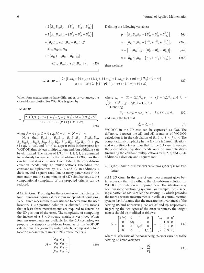
Distance-weighted (matrix inversion)Threshold (matrix inversion)LOP (matrix inversion)Distance-weighted (proposed WGDOP formulae)Threshold (proposed WGDOP formulae)LOP (proposed WGDOP formulae)

Figure 1: CDFs of the location error for various methods when fourmeasurements have different error variances (Type 1).

express; thus sixteen multiplications and four additionscan be eliminated. The value 𝜔 is also treated as a constantin the WGDOP calculation. From Table 2, this closed-form solution only needs 39 multiplications (including theconstant multiplication by 4, 2, 2, and 2), 44 additions, 1division, and 1 square root.

4.2.2. 2D Case. The WGDOP in the 2D case is expressedas (38). The WGDOP calculation in the 2D case requires 6multiplications and 6 additions fewer than that in the 3Dcase.The closed-form equation needs only 33 multiplications(including the constant multiplications by 4, 2, 2, and 2), 38additions, 1 division, and 1 square root. An alternative closed-form solution of theWGDOP calculation has been presentedin this paper, in which one measurement provides superiorlocation precision over the others.

5. Simulation Results

Time of arrival (TOA) is major time based method andusually used in calculating themobile station (MS) location incellular communication systems. It is consisting of seven basestations (BSs) in cellular communication system.The servingBS and its six neighboring BSs are separated by 5 km, and the

0 100 200 300 400 5000

0.1

0.2

0.3

0.4

0.5

0.6

0.7

0.8

0.9

1

Location error (m)CD

F

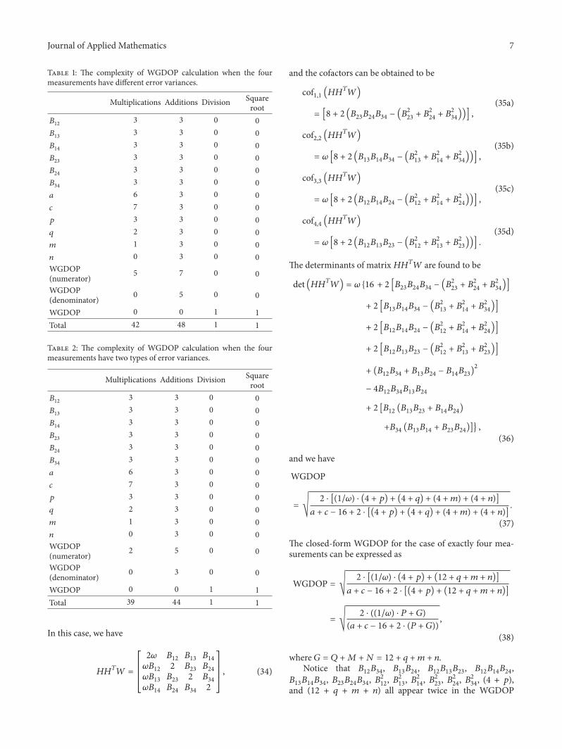
Distance-weighted (matrix inversion)Threshold (matrix inversion)LOP (matrix inversion)Distance-weighted (proposed WGDOP formulae)Threshold (proposed WGDOP formulae)LOP (proposed WGDOP formulae)

Figure 2: Comparison of CDFs of location error for variousmethods when fourmeasurements have two types of error variances(Type 2).

MS is randomly placed among the BSs [25]. The non-line-of-sight (NLOS) propagation model is based on the uniformlydistributed noise model [24], in which the TOANLOS errorsfrom all the BSs are different and assumed to be uniformlydistributed over (0, 𝑈

𝑖), for 𝑖 = 1, 2, . . . , 7 where 𝑈

𝑖is the

upper bound. For Type 1, the variables are chosen as follows:𝑈

1= 200m, 𝑈

2= 400m, 𝑈

3= 350m, 𝑈

4= 700m,

𝑈

5= 300m, 𝑈

6= 500m, and 𝑈

7= 350m. For Type 2, the

variables are given as follows: 𝑈1= 200m and 𝑈

𝑖= 500, for

𝑖 = 2, 3, . . . , 7. The diagonal elements of the weighted matrix𝑊 are utilized with the reciprocal of the square root of anupper bound of the NLOS errors.

In order to verify the superior properties of the proposedformulae, we compare the results of WGDOP calculationaccuracy for the proposed formulae and matrix inversionmethod. The WGDOP residual is defined as the differ-ence between the proposed formulae and matrix inversionmethod. Table 3 shows average WGDOP residual for theproposed formulae and Rprop-based algorithm. For Type 1and 2, the proposed formulae always provide much betterWGDOP residual than Rprop-based algorithm [23].

We can evaluate the positioning accuracy with minimumWGDOP algorithm; MS location can be estimated by the


0 100 200 300 400 500 600 7000

0.1

0.2

0.3

0.4

0.5

0.6

0.7

0.8

0.9

1

Location error (m)

CDF

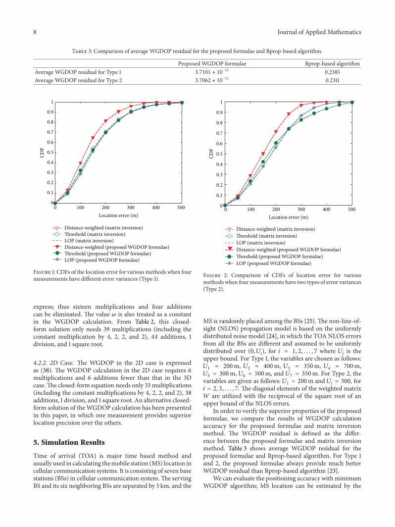
Distance-weighted (proposed WGDOP formulae)Threshold (proposed WGDOP formulae)LOP (proposed WGDOP formulae)Distance-weighted (selected randomly)Threshold (selected randomly)LOP (selected randomly)

Figure 3: Comparison of location error CDFs using the subsetwith proposed minimum WGDOP approximation and the subsetselected four BSs randomly (Type 1).

linear lines of position algorithm (LOP) [26], distance-weighted method, and threshold method which we haveproposed in [27]. When four measurements have differenterror variances (Type 1) or fourmeasurements have two typesof error variances (Type 2), the proposed WGDOP formulaeandmatrix inversionmethod provide the nearly identical MSlocation estimation, as shown in Figures 1 and 2.

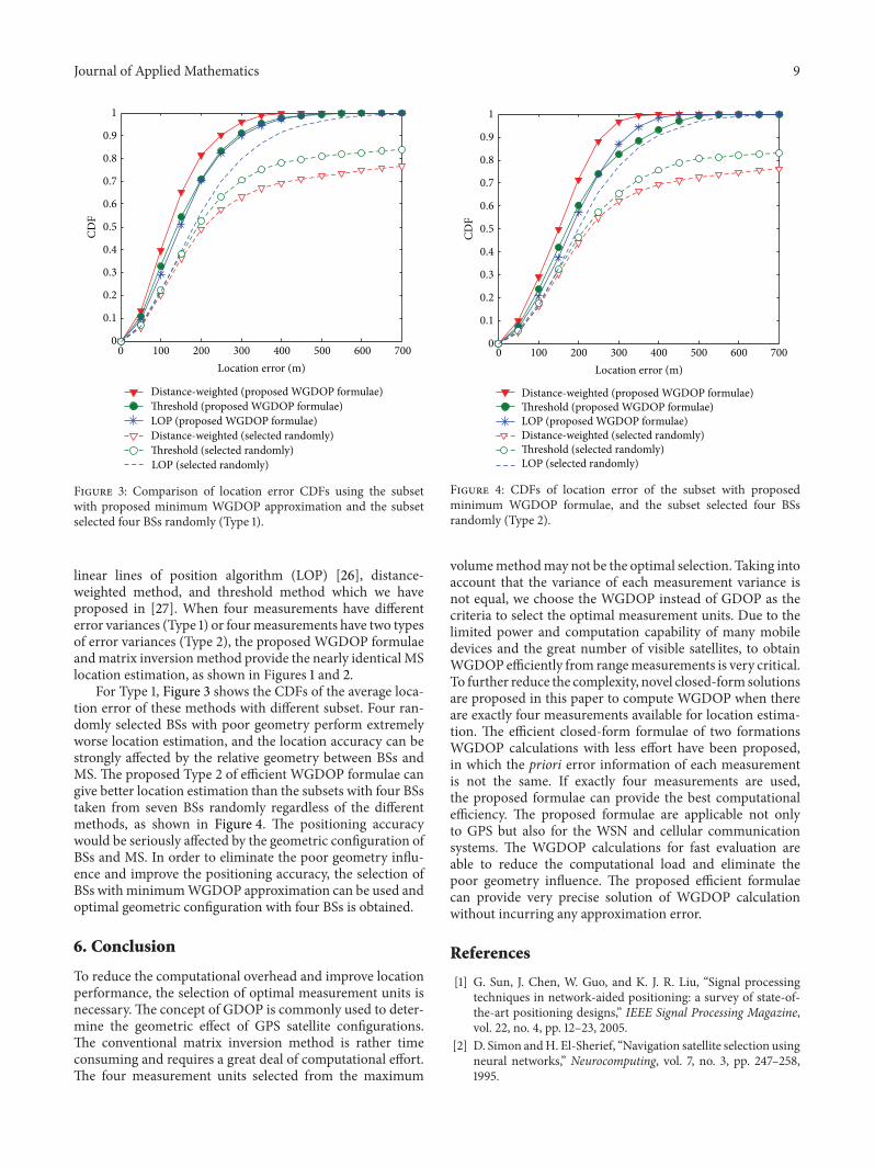
For Type 1, Figure 3 shows the CDFs of the average loca-tion error of these methods with different subset. Four ran-domly selected BSs with poor geometry perform extremelyworse location estimation, and the location accuracy can bestrongly affected by the relative geometry between BSs andMS. The proposed Type 2 of efficient WGDOP formulae cangive better location estimation than the subsets with four BSstaken from seven BSs randomly regardless of the differentmethods, as shown in Figure 4. The positioning accuracywould be seriously affected by the geometric configuration ofBSs and MS. In order to eliminate the poor geometry influ-ence and improve the positioning accuracy, the selection ofBSs withminimumWGDOP approximation can be used andoptimal geometric configuration with four BSs is obtained.

6. Conclusion

To reduce the computational overhead and improve locationperformance, the selection of optimal measurement units isnecessary. The concept of GDOP is commonly used to deter-mine the geometric effect of GPS satellite configurations.The conventional matrix inversion method is rather timeconsuming and requires a great deal of computational effort.The four measurement units selected from the maximum

0 100 200 300 400 500 600 7000

0.1

0.2

0.3

0.4

0.5

0.6

0.7

0.8

0.9

1

Location error (m)

CDF

Distance-weighted (proposed WGDOP formulae)Threshold (proposed WGDOP formulae)LOP (proposed WGDOP formulae)Distance-weighted (selected randomly)Threshold (selected randomly)LOP (selected randomly)

Figure 4: CDFs of location error of the subset with proposedminimum WGDOP formulae, and the subset selected four BSsrandomly (Type 2).

volumemethodmay not be the optimal selection. Taking intoaccount that the variance of each measurement variance isnot equal, we choose the WGDOP instead of GDOP as thecriteria to select the optimal measurement units. Due to thelimited power and computation capability of many mobiledevices and the great number of visible satellites, to obtainWGDOP efficiently from rangemeasurements is very critical.To further reduce the complexity, novel closed-form solutionsare proposed in this paper to compute WGDOP when thereare exactly four measurements available for location estima-tion. The efficient closed-form formulae of two formationsWGDOP calculations with less effort have been proposed,in which the priori error information of each measurementis not the same. If exactly four measurements are used,the proposed formulae can provide the best computationalefficiency. The proposed formulae are applicable not onlyto GPS but also for the WSN and cellular communicationsystems. The WGDOP calculations for fast evaluation areable to reduce the computational load and eliminate thepoor geometry influence. The proposed efficient formulaecan provide very precise solution of WGDOP calculationwithout incurring any approximation error.

References

[1] G. Sun, J. Chen, W. Guo, and K. J. R. Liu, “Signal processingtechniques in network-aided positioning: a survey of state-of-the-art positioning designs,” IEEE Signal Processing Magazine,vol. 22, no. 4, pp. 12–23, 2005.

[2] D. Simon andH. El-Sherief, “Navigation satellite selection usingneural networks,” Neurocomputing, vol. 7, no. 3, pp. 247–258,1995.


[3] D. Simon andH. El-Sherief, “Fault-tolerant training for optimalinterpolative nets,” IEEE Transactions on Neural Networks, vol.6, no. 6, pp. 1531–1535, 1995.

[4] D. E. Rumelhart, G. E. Hinton, and R. J. Williams, “Learningrepresentations by back-propagating errors,” Nature, vol. 323,no. 6088, pp. 533–536, 1986.

[5] D.-J. Jwo and K.-P. Chin, “Applying back-propagation neuralnetworks to GDOP approximation,” Journal of Navigation, vol.55, no. 1, pp. 97–108, 2002.

[6] C.-S. Chen and S.-L. Su, “Resilient back-propagation neuralnetwork for approximation 2-D GDOP,” in Proceedings ofthe International MultiConference of Engineers and ComputerScientists, vol. 2, pp. 900–904, March 2010.

[7] D. Y. Hsu, “Relations between dilutions of precision and volumeof the tetrahedron formed by four satellites,” in Proceedings ofthe IEEE Position Location and Navigation Symposium, pp. 669–676, April 1994.

[8] M. Kihara and T. Okada, “A satellite selection method andaccuracy for the global positioning system,” Navigation, vol. 31,no. 1, pp. 8–20, 1984.

[9] J. Zhu, “Calculation of geometric dilution of precision,” IEEETransactions on Aerospace and Electronic Systems, vol. 28, no. 3,pp. 893–894, 1992.

[10] E. D. Kaplan and C. J. Hegarty, Understanding GPS: Principlesand Applications, Artech House Press, Boston, Mass, USA,2006.

[11] M. Kihara, “Study of a GPS satellite selection policy to improvepositioning accuracy,” in Proceedings of the IEEE PositionLocation and Navigation Symposium, pp. 267–273, April 1994.

[12] G.M. Siouris,Aerospace Avionics Systems—AModern Synthesis,Academic Press, San Diego, Calif, USA, 1993.

[13] C. Park, I. Kim, J. G. Lee, and G.-I. Jee, “A satellite selectioncriterion incorporating the effect of elevation angle in GPSpositioning,” Control Engineering Practice, vol. 4, no. 12, pp.1741–1746, 1996.

[14] H. Sairo, D. Akopian, and J. Takala, “Weighted dilution of preci-sion as qualitymeasure in satellite positioning,” IEE Proceedings,vol. 150, no. 6, pp. 430–436, 2003.

[15] Y. Yong and M. Lingjuan, “GDOP results in all-in-view posi-tioning and in four optimum satellites positioning with GPSPRN codes ranging,” in Proceedings of the Position Location andNavigation Symposium, pp. 723–727, April 2004.

[16] M. Pachter, J. Amt, and J. Raquet, “Accurate positioning usinga planar pseudolite array,” in Proceedings of the IEEE/IONPosition, Location and Navigation Symposium, pp. 433–440,May 2008.

[17] K. Kawamura and T. Tanaka, “Study on the improvement ofmeasurement accuracy in GPS,” in Proceedings of the SICE-ICASE International Joint Conference, pp. 1372–1375, October2006.

[18] B. Xu and S. Bingjun, “Satellite selection algorithm for com-bined gpsgalileo navigation receiver,” in Proceedings of the 4thInternational Conference on Autonomous Robots and Agents, pp.149–154, February 2009.

[19] C.Hongwei and S. Zhongkang, “Anonlinear optimized locationalgorithm for bistatic radar system,” in Proceedings of the IEEENational Aerospace and Electronics Conference, vol. 1, pp. 201–205, May 1995.

[20] N. Levanon, “Lowest GDOP in 2-D scenarios,” IEE Proceedings,vol. 147, no. 3, pp. 149–155, 2000.

[21] H. Lu and X. Liu, “Compass augmented regional constellationoptimization by a multi-objective algorithm based on decom-position and PSO,” Chinese Journal of Electronics, vol. 21, no. 2,pp. 374–378, 2012.

[22] M. Zhang, J. Zhang, and Y. Qin, “Satellite selection for multi-constellation,” in Proceedings of the IEEE/ION Position, Locationand Navigation Symposium, pp. 1053–1059, May 2008.

[23] C.-S. Chen, J.-M. Lin, and C.-T. Lee, “Neural network forWGDOP approximation and mobile location,” MathematicalProblems in Engineering, vol. 2013, Article ID 369694, 11 pages,2013.

[24] S. Venkatraman, J. Caffery Jr., and H.-R. You, “A novel ToAlocation algorithm using LoS range estimation for NLoS envi-ronments,” IEEE Transactions on Vehicular Technology, vol. 53,no. 5, pp. 1515–1524, 2004.

[25] J. Caffery Jr. and G. Stuber, “Subscriber location in CDMAcellular networks,” IEEE Transactions on Vehicular Technology,vol. 47, pp. 406–416, 1998.

[26] J. J. Caffery Jr., “A new approach to the geometry of TOAlocation,” in Proceedings of the 52nd Vehicular TechnologyConference, pp. 1943–1949, September 2000.

[27] C.-S. Chen, S.-L. Su, and Y.-F. Huang, “Hybrid TOA/AOAgeometrical positioning schemes for mobile location,” IEICETransactions on Communications, vol. E92-B, no. 2, pp. 396–402, 2009.

Submit your manuscripts athttp://www.hindawi.com

Hindawi Publishing Corporationhttp://www.hindawi.com Volume 2014

MathematicsJournal of


Mathematical Problems in Engineering

Hindawi Publishing Corporationhttp://www.hindawi.com

Differential EquationsInternational Journal of

Volume 2014

Applied MathematicsJournal of


Probability and StatisticsHindawi Publishing Corporationhttp://www.hindawi.com Volume 2014

Journal of


Mathematical PhysicsAdvances in

Complex AnalysisJournal of


OptimizationJournal of


CombinatoricsHindawi Publishing Corporationhttp://www.hindawi.com Volume 2014

International Journal of


Operations ResearchAdvances in

Journal of


Function Spaces

Abstract and Applied AnalysisHindawi Publishing Corporationhttp://www.hindawi.com Volume 2014

International Journal of Mathematics and Mathematical Sciences


The Scientific World JournalHindawi Publishing Corporation http://www.hindawi.com Volume 2014


Algebra

Discrete Dynamics in Nature and Society



Decision SciencesAdvances in

Discrete MathematicsJournal of

Hindawi Publishing Corporationhttp://www.hindawi.com

Volume 2014 Hindawi Publishing Corporationhttp://www.hindawi.com Volume 2014

Stochastic AnalysisInternational Journal of

Documents

Research Article Calculation of Weighted Geometric ...downloads.hindawi.com/journals/jam/2013/953048.pdf · Research Article Calculation of Weighted Geometric Dilution of Precision