Embed Size (px)
Citation preview
Research ArticleAn Operational Matrix of Fractional Differentiation of theSecond Kind of Chebyshev Polynomial for Solving MultitermVariable Order Fractional Differential Equation
Jianping Liu Xia Li and Limeng Wu
Hebei Normal University of Science and Technology Qinhuangdao Hebei 066004 China
Correspondence should be addressed to Jianping Liu liujianping0408126com
Received 30 March 2016 Revised 29 April 2016 Accepted 4 May 2016
Academic Editor Jose A Tenereiro Machado
Copyright copy 2016 Jianping Liu et al This is an open access article distributed under the Creative Commons Attribution Licensewhich permits unrestricted use distribution and reproduction in any medium provided the original work is properly cited
The multiterm fractional differential equation has a wide application in engineering problems Therefore we propose a method tosolvemultiterm variable order fractional differential equation based on the second kind of Chebyshev PolynomialThemain idea ofthis method is that we derive a kind of operational matrix of variable order fractional derivative for the second kind of ChebyshevPolynomial With the operational matrices the equation is transformed into the products of several dependent matrices whichcan also be viewed as an algebraic system by making use of the collocation points By solving the algebraic system the numericalsolution of original equation is acquired Numerical examples show that only a small number of the second kinds of ChebyshevPolynomials are needed to obtain a satisfactory result which demonstrates the validity of this method
1 Introduction
The concept of fractional order derivative goes back to the17th century [1 2] It is only a few decades ago that itwas realized that the arbitrary order derivative provides anexcellent framework formodeling the real-world problems ina variety of disciplines from physics chemistry biology andengineering such as viscoelasticity and damping diffusionand wave propagation and chaos [3ndash6]
Orthogonal functions have received noticeable consid-eration for solving fractional differential equation (FDE)By using orthogonal functions the FDE can be reduced tosolve an algebraic system and then original problems aresimplified Ahmadian et al [7] proposed a computationalmethod based on Jacobi Polynomials for solving fuzzy linearFDE on interval [0 1] Kazem et al [8] constructed a generalformulation for the fractional order Legendre functionsYuzbası [9] gave the numerical solutions of fractional Riccatitype differential equations by means of the Bernstein Polyno-mials Kazem [10] constructed a general formulation for theJacobi operational matrix for fractional integral equations
Taumethod and collocationmethod arewidely used toolsfor the solution of FDE Operational approach of the taumethod was employed for solving fractional problems [11]A numerical approach was provided for the FDE based ona spectral tau method [12] An efficient method based onthe shifted Chebyshev-tau idea was presented for solvingthe space fractional diffusion equations [13] Tau method isvery effective for constant coefficient nonlinear problemsbut the method is not generally adopted for nonlinear FDEIn practice since collocation method has the advantages ofless computation and easy implementation it is more widelyapplied for solving variable coefficient nonlinear problemsThe collocation method was used for solving the nonlinearfractional integrodifferential equations [14] The third kindof Chebyshev wavelets collocation method was introducedfor solving the time fractional convection diffusion equationswith variable coefficients [15]
From the literatures above we conclude that manyauthors employed tau and collocation method for solvingdifferent kinds of FDE based on different kinds of orthogonalfunctions or their variants However for the aforementioned
Hindawi Publishing CorporationMathematical Problems in EngineeringVolume 2016 Article ID 7126080 10 pageshttpdxdoiorg10115520167126080
2 Mathematical Problems in Engineering
FDE the derivative order is a fixed constant which does notchange spatially and temporally variable order multitermFDE is not mentioned and solved Therefore our main moti-vation is to give a numerical technology for solving variableorder linear and nonlinear multiterm FDE based on thesecond kind of Chebyshev Polynomial With further devel-opment of science research it is found that variable orderfractional calculus can provide an effective mathematicalframework for the complex dynamical problemsThemodel-ing and application of variable order differential equation hasbeen a front subject In addition the FDE is a special case ofvariable order ones so it can also be solved by our proposedtechnology
Variable order derivative is proposed by Samko and Ross[16] in 1993 and then Lorenzo and Hartley [17 18] studiedvariable order calculus in theory more deeply Coimbraand Diaz [19 20] used variable order derivative to researchnonlinear dynamics and control problems of viscoelasticityoscillator Pedro et al [21] researched diffusive-convectiveeffects on the oscillatory flow past a sphere by variable ordermodelingThe development of numerical algorithms to solvevariable order FDE is necessary
Since the kernel of the variable order operators is verycomplex for having a variable exponent it is difficult to gainthe solution of variable order differential equation Only afew authors studied numerical methods of variable orderfractional differential equations Coimbra [19] employed aconsistent approximationwith first-order accurate for solvingvariable order differential equations Sun et al [22] proposeda second-order Runge-Kuttamethod to numerically integratethe variable order differential equation Lin et al [23] stud-ied the stability and the convergence of an explicit finite-difference approximation for the variable order fractionaldiffusion equation with a nonlinear source term Chen et al[24 25] paid their attention to Bernstein Polynomials to solvevariable order linear cable equation and variable order timefractional diffusion equation A numerical method based onthe Legendre Polynomials is presented for a class of variableorder FDE [26] Chen et al [27] introduced the numericalsolution for a class of nonlinear variable order FDE withLegendre wavelets
To the best of our knowledge it is not seen that opera-tional matrix of variable order derivative based on the secondkind of Chebyshev Polynomial is used to solve multitermvariable order FDE In addition for most literatures theysolved variable order FDE defined on the interval [0 1]Accordingly based on the second kind of Chebyshev Polyno-mial we propose a new efficient technique for solving mul-titerm variable order FDE defined on the interval [0 119877]
The multiterm variable order FDE is given as follows
119863120572(119905)
119891 (119905)
= 119865 (119905 119891 (119905) 1198631205731(119905)
119891 (119905) 1198631205732(119905)
119891 (119905) 119863120573119896(119905)
119891 (119905))
0 lt 119905 lt 119877
(1)
where 119863120572(119905)
119891(119905) and 119863120573119894(119905)
119891(119905) are fractional derivative inCaputo sense When 120572(119905) and 120573
119894(119905) 119894 = 1 2 119896 are all
constants (1) becomes (2) namely
119863120572
119891 (119905)
= 119865 (119905 119891 (119905) 1198631205731119891 (119905) 119863
1205732119891 (119905) 119863
120573119896119891 (119905))
0 lt 119905 lt 119877
(2)
Thus (2) is a special case of (1) Our proposed methodcan solve both (1) and (2) They often appear in oscillatoryequations such as vibration equation fractional Van Der Polequation the Rayleigh equationwith fractional damping andfractional Riccati differential equation
The basic idea of this method is that we derive differentialoperational matrices based on the second kind of ChebyshevPolynomial With the operational matrices the equation istransformed into the products of several dependent matriceswhich can also be viewed as an algebraic system by makinguse of the collocation points By solving the algebraic systemthe numerical solution is acquired Since the second kindsof Chebyshev Polynomials are orthogonal to each otherthe operational matrices based on Chebyshev Polynomialsgreatly reduce the size of computational work while accu-rately providing the series solution From some numericalexamples we can see that our results are in good agreementwith the analytical solution which demonstrates the validityof this methodTherefore it has the potential to utilize widerapplicability
The paper is organized as follows In Section 2 somenecessary definitions and properties of the variable orderfractional derivatives are introduced The basic definitionsof the second kind of Chebyshev Polynomial and functionapproximation are given in Sections 3 and 4 respectively InSection 5 a kind of operational matrix of the second kindof Chebyshev Polynomial is derived and then we appliedthe operational matrices to solve the equation as given atbeginning In Section 6 we present some numerical examplesto demonstrate the efficiency of the method We end thepaper with a few concluding remarks in Section 7
2 Basic Definition of Caputo Variable OrderFractional Derivatives
Definition 1 Caputo variable fractional derivative with order120572(119905) is defined by
119863120572(119905)
119906 (119905) =1
Γ (1 minus 120572 (119905))int119905
0+
(119905 minus 120591)minus120572(119905)
1199061015840
(120591) 119889120591
+(119906 (0+) minus 119906 (0minus)) 119905
minus120572(119905)
Γ (1 minus 120572 (119905))
(3)
If we assume the starting time in a perfect situation wecan get Definition 2 as follows
Mathematical Problems in Engineering 3
Definition 2 Consider
119863120572(119905)
119906 (119905) =1
Γ (1 minus 120572 (119905))int119905
0
(119905 minus 120591)minus120572(119905)
1199061015840
(120591) 119889120591
(0 lt 120572 (119905) lt 1)
(4)
By Definition 2 we can get the following formula [25]
119863120572(119905)
119905(119905119899
) =
Γ (119899 + 1)
Γ (119899 + 1 minus 120572 (119905))119905119899minus120572(119905)
119899 = 1 2
0 119899 = 0
(5)
3 Shifted Second Kind ofChebyshev Polynomial
The second kind of Chebyshev Polynomial defined on theinterval 119868 = [minus1 1] is orthogonal based on the weight func-tion 120596(119909) = radic1 minus 1199092 They satisfy the following formulas
1198800(119909) = 1
1198801(119909) = 2119909
119880119899+1
(119909) = 2119909119880119899(119909) minus 119880
119899minus1(119909)
119899 = 1 2
int1
minus1
radic1 minus 1199092119880119899(119909)119880119898(119909) 119889119909 =
0 119898 = 119899
120587
2 119898 = 119899
(6)
When 119905 isin [0 119877] let 119909 = 2119905119877 minus 1 we can get shifted secondkind of Chebyshev Polynomial
119899(119905) = 119880
119899(2119905119877 minus 1) whose
weight function is 120596(119905) = radic119905119877 minus 1199052 with 119905 isin [0 119877] They sat-isfy the following formulas
0(119905) = 1
1(119905) = 2 (
2119905
119877minus 1) =
4119905
119877minus 2
119899+1
(119905) = 2 (2119905
119877minus 1)
119899(119905) minus
119899minus1(119905)
119899 = 1 2 3
int119877
0
radic119905119877 minus 1199052119899(119905) 119898(119905) 119889119905 =
0 119898 = 119899
120587
81198772
119898 = 119899
(7)
The shifted second kind of Chebyshev Polynomial 119899(119905)
can also be expressed as
119899(119905)
=
1 119899 = 0
[1198992]
sum119896=0
(minus1)119896
(119899 minus 119896)
119896 (119899 minus 2119896)(4119905
119877minus 2)119899minus2119896
119899 ge 1
(8)
where [1198992] denotes the maximum integer which is no morethan 1198992
Let
Ψ (119905) = [0(119905)
1(119905)
119899(119905)]119879
119879 (119905) = [1 119905 119905119899
]119879
(9)
then
Ψ (119905) = 119860119879 (119905) (10)
Let
119860 = 119861119862 (11)
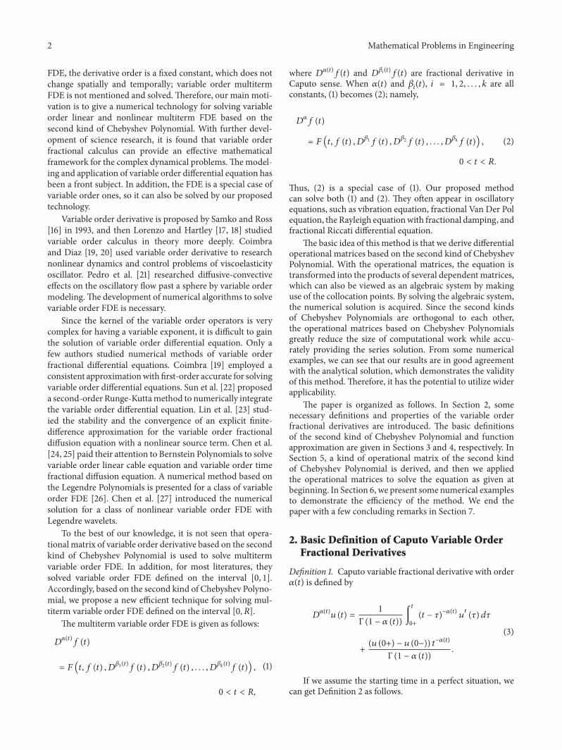
If 119899 is an even number then
119861
=
[[[[[[[[[[[[[[[[[[[[[
[
1 0 0 sdot sdot sdot 0
0 (minus1)0
(1 minus 0)
0 (1 minus 0)(4
119877)1minus0
0 sdot sdot sdot 0
(minus1)1
(2 minus 1)
1 (2 minus 2)(4
119877)2minus2
0 (minus1)0
(2 minus 0)
0 (2 minus 0)(4
119877)2minus0
sdot sdot sdot 0
(minus1)1198992
(119899 minus 1198992)
(1198992) (119899 minus 2 sdot 1198992)(4
119877)119899minus2sdot1198992
sdot sdot sdot (minus1)1198992minus1
(119899 minus 1198992 + 1)
(1198992 minus 1) [119899 minus 2 (1198992 minus 1)](4
119877)119899minus2(1198992minus1)
sdot sdot sdot (minus1)0
(119899 minus 0)
0 (119899 minus 0)(4
119877)119899minus0
]]]]]]]]]]]]]]]]]]]]]
]
(12)
4 Mathematical Problems in Engineering
If 119899 is an odd number then
119861
=
[[[[[[[[[[[[[[
[
1 0 0 sdot sdot sdot 0
0 (minus1)0
(1 minus 0)
0 (1 minus 0)(4
119877)1minus0
0 sdot sdot sdot 0
(minus1)1
(2 minus 1)
1 (2 minus 2)(4
119877)2minus2
0 (minus1)0
(2 minus 0)
0 (2 minus 0)(4
119877)2minus0
sdot sdot sdot 0
0 (minus1)(119899minus1)2
(119899 minus (119899 minus 1) 2)
((119899 minus 1) 2) (119899 minus 2 sdot (119899 minus 1) 2)(4
119877)119899minus2sdot(119899minus1)2
0 sdot sdot sdot (minus1)0
(119899 minus 0)
0 (119899 minus 0)(4
119877)119899minus0
]]]]]]]]]]]]]]
]
119862 =
[[[[[[[[[[[[[[[[[[
[
1 0 0 sdot sdot sdot 0
(1
0)(minus
119877
2)1minus0
(1
1)(minus
119877
2)1minus1
0 sdot sdot sdot 0
(2
0)(minus
119877
2)2minus0
(2
1)(minus
119877
2)2minus1
(2
2)(minus
119877
2)2minus2
sdot sdot sdot 0
(119899
0)(minus
119877
2)119899minus0
(119899
1)(minus
119877
2)119899minus1
(119899
2)(minus
119877
2)119899minus2 (
119899
119899)(minus
119877
2)119899minus119899
]]]]]]]]]]]]]]]]]]
]
(13)
Therefore we can easily gain
119879119899(119905) = 119860
minus1
Ψ (119905) (14)
4 Function Approximation
Theorem 3 Assume a function 119891(119905) isin [0 119877] be 119899 times con-tinuously differentiable Let 119906
119899(119905) = sum
119899
119894=0120582119894119894(119905) = Λ
119879
Ψ119899(119905)
be the best square approximation function of 119891(119905) where Λ =
[1205820 1205821 120582
119899]119879 and Ψ
119899(119905) = [
0(119905) 1(119905)
119899(119905)]119879 then
1003817100381710038171003817119891 (119905) minus 119906119899(119905)
1003817100381710038171003817 le119872119878119899+1
119877
(119899 + 1)radic120587
8 (15)
where119872 = max119905isin[0119877]
119891(119899+1)
(119905) and 119878 = max119877 minus 1199050 1199050
Proof We consider the Taylor Polynomial
119891 (119905) = 119891 (1199050) + 1198911015840
(1199050) (119905 minus 119905
0) + sdot sdot sdot
+ 119891(119899)
(1199050)(119905 minus 1199050)119899
119899+ 119891(119899+1)
(120578)(119905 minus 1199050)119899+1
(119899 + 1)
1199050isin [0 119877]
(16)
where 120578 is between 119905 and 1199050
Let119901119899(119905) = 119891 (119905
0) + 1198911015840
(1199050) (119905 minus 119905
0) + sdot sdot sdot
+ 119891(119899)
(1199050)(119905 minus 1199050)119899
119899
(17)
then
1003816100381610038161003816119891 (119909) minus 119901119899(119909)
1003816100381610038161003816 =
1003816100381610038161003816100381610038161003816100381610038161003816
119891(119899+1)
(120578)(119905 minus 1199050)119899+1
(119899 + 1)
1003816100381610038161003816100381610038161003816100381610038161003816
(18)
Since 119906119899(119905) = sum
119899
119894=0120582119894119894(119905) = Λ
119879
Ψ119899(119905) is the best square
approximation function of 119891(119905) we can gain1003817100381710038171003817119891 (119905) minus 119906
119899(119905)
10038171003817100381710038172
le1003817100381710038171003817119891 (119905) minus 119901
119899(119905)
10038171003817100381710038172
= int119877
0
120596 (119905) [119891 (119905) minus 119901119899(119905)]2
119889119905
= int119877
0
120596 (119905) [119891(119899+1)
(120578)(119905 minus 1199050)119899+1
(119899 + 1)]
2
119889119905
le1198722
[(119899 + 1)]2int119877
0
(119905 minus 1199050)2119899+2
120596 (119905) 119889119905
=1198722
[(119899 + 1)]2int119877
0
(119905 minus 1199050)2119899+2radic119905119877 minus 1199052119889119905
(19)
Let 119878 = max119877 minus 1199050 1199050 therefore
1003817100381710038171003817119891 (119905) minus 119906119899(119905)
10038171003817100381710038172
le1198722
1198782119899+2
[(119899 + 1)]2int119877
0
radic119905119877 minus 1199052119889119905
=1198722
1198782119899+2
[(119899 + 1)]2
1205871198772
8
(20)
Andby taking the square rootsTheorem3 can be proved
5 Operational Matrices of 119863120572(119905)Ψ119899(119905) and
119863120573119894(119905)
Ψ119899(119905) 119894 = 1 2 119896 Based on Shifted
Second Kind of Chebyshev Polynomial
Consider
119863120572(119905)
Ψ119899(119905) = 119863
120572(119905)
[119860119879119899(119905)] = 119860119863
120572(119905)
[1 119905 sdot sdot sdot 119905119899
]119879
(21)
Mathematical Problems in Engineering 5
According to (5) we can get
119863120572(119905)
Ψ119899(119905)
= 119860[0Γ (2)
Γ (2 minus 120572 (119905))1199051minus120572(119905)
sdot sdot sdotΓ (119899 + 1)
Γ (119899 + 1 minus 120572 (119905))119905119899minus120572(119905)
]
119879
= 119860
[[[[[[[[[
[
0 0 sdot sdot sdot 0
0Γ (2)
Γ (2 minus 120572 (119905))119905minus120572(119905)
sdot sdot sdot 0
0 0 sdot sdot sdotΓ (119899 + 1)
Γ (119899 + 1 minus 120572 (119905))119905minus120572(119905)
]]]]]]]]]
]
[[[[[[
[
1
119905
119905119899
]]]]]]
]
= 119860119872119860minus1
Ψ119899(119905)
(22)
where
119872
=
[[[[[[[[[
[
0 0 sdot sdot sdot 0
0Γ (2)
Γ (2 minus 120572 (119905))119905minus120572(119905)
sdot sdot sdot 0
0 0 sdot sdot sdotΓ (119899 + 1)
Γ (119899 + 1 minus 120572 (119905))119905minus120572(119905)
]]]]]]]]]
]
(23)
119860119872119860minus1 is called the operational matrix of119863120572(119905)Ψ
119899(119905) There-
fore
119863120572(119905)
119891 (119905) asymp 119863120572(119905)
(Λ119879
Ψ119899(119905)) = Λ
119879
119863120572(119905)
Ψ119899(119905)
= Λ119879
119860119872119860minus1
Ψ119899(119905)
(24)
Similarly we can get
119863120573119894(119905)
Ψ119899(119905) = 119860119873
119894119860minus1
Ψ119899(119905) 119894 = 1 2 119896 (25)
where119873119894
=
[[[[[[[[[[
[
0 0 sdot sdot sdot 0
0Γ (2)
Γ (2 minus 120573119894(119905))
119905minus120573119894(119905)
sdot sdot sdot 0
0 0 sdot sdot sdotΓ (119899 + 1)
Γ (119899 + 1 minus 120573119894(119905))
119905minus120573119894(119905)
]]]]]]]]]]
]
(26)
119860119873119894119860minus1 is called the operational matrix of119863120573119894(119905)Ψ
119899(119905) Thus
119863120573119894(119905)
119891 (119905) asymp 119863120573119894(119905)
(Λ119879
Ψ119899(119905)) = Λ
119879
119863120573119894(119905)
Ψ119899(119905)
= Λ119879
119860119873119894119860minus1
Ψ119899(119905)
(27)
The original equation (1) is transformed into the form asfollows
Λ119879
119860119872119860minus1
Ψ119899(119905) = 119865 [119905 Λ
119879
Ψ119899(119905) Λ
119879
1198601198731119860minus1
Ψ119899(119905)
Λ119879
119860119873119896119860minus1
Ψ119899(119905)] 119905 isin [0 119877]
(28)
In this paper we use collocation method to solve the coef-ficientΛ = [120582
0 1205821 120582
119899]119879 By taking the collocation points
(28) will become an algebraic system We can gain thesolution Λ = [120582
0 1205821 120582
119899]119879 by Newton method Finally
the numerical solution 119906119899(119905) = Λ
119879
Ψ119899(119905) is gained
6 Numerical Examples and Results Analysis
In this section we verify the efficiency of proposedmethod tosupport the above theoretical discussion For this purpose weconsider linear and nonlinear multiterm variable order FDEand corresponding multiterm FDE For multiterm variableorder FDE we compare our approach with the analyticalsolution For multiterm FDE we compare our computationalresults with the analytical solution and solutions in [28] byusing other methods The results indicate that our methodis a powerful tool for solving multiterm variable order FDEand multiterm FDE Numerical examples show that only asmall number of the second kinds of Chebyshev Polynomialsare needed to obtain a satisfactory result Furthermore ourmethod has higher precision than [28] In this section thenotation
120576 = max119894=01119899
1003816100381610038161003816119891 (119905119894) minus 119906119899(119905119894)1003816100381610038161003816
119905119894= 119877
(2119894 + 1)
2 (119899 + 1) 119894 = 0 1 119899
(29)
is used to show the accuracy of our proposed method
Example 1 (a) Consider the linear FDE with variable orderas follows
119886119863120572(119905)
119891 (119905) + 119887 (119905)1198631205731(119905)
119891 (119905) + 119888 (119905)1198631205732(119905)
119891 (119905)
+ 119890 (119905)1198631205733(119905)
119891 (119905) + 119896 (119905) 119891 (119905) = 119892 (119905)
119905 isin [0 119877]
119910 (0) = 2
1199101015840
(0) = 0
(30)
where
119891 (119905) = minus1198861199052minus120572(119905)
Γ (3 minus 120572 (119905))minus 119887 (119905)
1199052minus1205731(119905)
Γ (3 minus 1205731(119905))
minus 119888 (119905)1199052minus1205732(119905)
Γ (3 minus 1205732(119905))
minus 119890 (119905)1199052minus1205733(119905)
Γ (3 minus 1205733(119905))
+ 119896 (119905) (2 minus1199052
2)
(31)
The analytical solution is119891(119905) = 2minus1199052
2We use our proposedtechnology to solve it
6 Mathematical Problems in Engineering
0 02 04 06 08 116
17
18
19
2
t
f(t)
Analytical solutionNumerical solution
R = 1 n = 3
(a)
0 1 2 3 4minus5
minus4
minus3
minus2
minus1
0
1
2
t
f(t)
Analytical solutionNumerical solution
R = 4 n = 6
(b)
Figure 1 Analytical solution and numerical solution of Example 1(a) for different 119877
Let119891(119905) asymp 119906119899(119905) = Λ
119879
Ψ119899(119905)120572(119905) = 2119905120573
1(119905) = 1199053120573
2(119905) =
1199054 and 1205733(119905) = 1199055 according to (28) we have
119886Λ119879
119860119872119860minus1
Ψ119899(119905) + 119887 (119905) Λ
119879
1198601198731119860minus1
Ψ119899(119905)
+ 119888 (119905) Λ119879
1198601198732119860minus1
Ψ119899(119905)
+ 119890 (119905) Λ119879
1198601198733119860minus1
Ψ119899(119905) + 119896 (119905) Λ
119879
Ψ119899(119905)
= 119892 (119905)
(32)
Take the collocation points 119905119894= 119877((2119894 + 1)2(119899 + 1)) 119894 = 0 1
119899 to process (32) and then get
119886Λ119879
119860119872119860minus1
Ψ119899(119905119894) + 119887 (119905
119894) Λ119879
1198601198731119860minus1
Ψ119899(119905119894)
+ 119888 (119905119894) Λ119879
1198601198732119860minus1
Ψ119899(119905119894)
+ 119890 (119905119894) Λ119879
1198601198733119860minus1
Ψ119899(119905119894) + 119896 (119905
119894) Λ119879
Ψ119899(119905119894)
= 119892 (119905119894) 119894 = 1 2 119899
(33)
By solving the algebraic system (33) we can gain the vec-tor Λ = [120582
0 1205821 120582
119899]119879 Subsequently numerical solution
119906119899(119905) = Λ
119879
Ψ119899(119905) is obtained Likely [28] we present numer-
ical solution by our method for
119886 = 1
119887 (119905) = radic119905
119888 (119905) = 11990513
119890 (119905) = 11990514
119896 (119905) = 11990515
(34)
Table 1 Values of 120576 of Example 1(a) for different 119877
119877 119899 = 3 119899 = 4 119899 = 5 119899 = 6
119877 = 1 0 22204119890 minus 16 22204119890 minus 16 33529119890 minus 14
119877 = 2 0 44409119890 minus 16 13323119890 minus 15 95812119890 minus 14
119877 = 4 22204119890 minus 16 35527119890 minus 15 31974119890 minus 14 61018119890 minus 13
In Table 1 we list the values of 120576 at the collocationpoints From Table 1 we could find that a small number ofChebyshev Polynomials are needed to reach perfect solutionfor different 119877 Figure 1 shows the analytical solution andnumerical solution for different 119877 at collocation points Wecan conclude that the numerical solution is very close tothe analytical solution The same trend is observed for othervalues of 120572(119905) and 120573
119894(119905) 119894 = 1 2 119896 All the values of 120576 are
small enough to meet the practical engineering applicationLet 120572(119905) = 2 120573
1(119905) = 1234 120573
2(119905) = 1 120573
3(119905) = 0333 and
119877 = 1 as [28] Example 1(a) becomes a multiterm order FDEnamely Example 1(b) This problem has been solved in [28]
(b) See [28]
1198861198632
119891 (119905) + 119887 (119905)1198631205731119891 (119905) + 119888 (119905)119863119891 (119905)
+ 119890 (119905)1198631205733119891 (119905) + 119896 (119905) 119891 (119905) = 119892 (119905) 119905 isin [0 1]
119910 (0) = 2
1199101015840
(0) = 0
(35)
where
119891 (119905) = minus119886 minus 119887 (119905)1199052minus1205731
Γ (3 minus 1205731)minus 119888 (119905) 119905
minus 119890 (119905)1199052minus1205733
Γ (3 minus 1205733)+ 119896 (119905) (2 minus
1199052
2)
(36)
Mathematical Problems in Engineering 7
Table 2 Computational results of Example 1(b) for 119877 = 1
119905 Λ 120576
119899 = 3 [18438 minus01250 minus00313 minus00000]119879 44409119890 minus 16
119899 = 4 [18438 minus01250 minus00312 00000 minus00000]119879 14633119890 minus 13
119899 = 5 [18437 minus01250 minus00313 00000 minus00000 00000]119879 32743119890 minus 12
119899 = 6 [18438 minus01250 minus00312 00000 00000 00000 minus00000]119879 10725119890 minus 13
Table 3 Values of 120576 of Example 2(b) for 119877 = 2 4
119877 119899 = 3 119899 = 4 119899 = 5 119899 = 6
119877 = 2 88818119890 minus 16 91038119890 minus 15 22959119890 minus 13 94480119890 minus 14
119877 = 4 88818119890 minus 16 10214119890 minus 14 73275119890 minus 15 38369119890 minus 13
The analytical solution is 119891(119905) = 2 minus 1199052
2 Example 1(b) isa special case of Example 1(a) so we still obtain the solutionby ourmethod as Example 1(a)The computational results areseen in Table 2 We list the vector Λ = [120582
0 1205821 120582
119899]119879 and
the values of 120576 at the collocation points
As seen from Table 2 the vector Λ = [1205820 1205821 120582
119899]119879
obtained is mainly composed of three terms namely 1205820 1205821
1205822 which is in agreement with the analytical solution 119891(119905) =
2minus1199052
2The values of 120576 are smaller than [28]with the same sizeof Chebyshev Polynomials (in [28] the value of 120576 is 688384119890minus5 for 119899 = 5) In addition we extend the interval from [0 1] to[0 2] and [0 4] Similarly we also get the perfect results asshown in Table 3 which is not solved in [28]
Example 2 (a) As the second example the nonlinear multi-term variable order FDE
119863120572(119905)
119891 (119905) + 1198631205731(119905)
119891 (119905)1198631205732(119905)
119891 (119905) + 1198912
(119905) = 119892 (119905)
119905 isin [0 119877] (37)
with
119892 (119905) = 1199056
+6
Γ (4 minus 120572 (119905))1199053minus120572(119905)
+36
Γ (4 minus 1205731(119905)) Γ (4 minus 120573
2(119905))
1199056minus1205731(119905)minus1205732(119905)
(38)
subject to the initial conditions 119891(0) = 1198911015840
(0) = 11989110158401015840
(0) = 0 isconsidered The analytical solution is 119891(119905) = 119905
3Let 119891(119905) = Λ
119879
Ψ(119905) according to (28) we have
119886Λ119879
119860119872119860minus1
Ψ119899+ (Λ119879
1198601198731119860minus1
Ψ119899) (Λ119879
1198601198732119860minus1
Ψ119899)
+ (Λ119879
Ψ119899)2
= 119892 (119905)
(39)
Let 120572(119905) = 1199052 1205731(119905) = sin 119905 and 120573
2(119905) = 1199054 by taking
the collocation points the solution of Example 2(a) couldbe gained The values of 120576 are displayed in Table 4 for dif-ferent 119877 From the result analysis our method could gainsatisfactory solution Figure 2 obviously shows that the num-erical solution converges to the analytical solution
Table 4 Values of 120576 of Example 2(a) with 120572(119905) = 1199052 1205731(119905) = sin 119905
and 1205732(119905) = 1199054
119877 119899 = 3 119899 = 4 119899 = 5 119899 = 6
119877 = 1 51560119890 minus 15 22690119890 minus 14 54114119890 minus 14 10227119890 minus 13
119877 = 2 18874119890 minus 15 14660119890 minus 14 66386119890 minus 14 74174119890 minus 13
119877 = 4 43512119890 minus 15 31200119890 minus 14 51616119890 minus 08 10565119890 minus 11
If 120572(119905) 1205731(119905) 1205732(119905) are constants Example 2(a) becomes a
multiterm order FDE in [28]This problem for 119877 = 1 has alsobeen solved in [28]
(b) See [28]
119863120572
119891 (119905) + 1198631205731119891 (119905)119863
1205732119891 (119905) + 119891
2
(119905) = 119892 (119905)
2 lt 120572 lt 3 1 lt 1205731lt 2 0 lt 120573
2lt 1 119905 isin [0 1]
(40)
with
119892 (119905) = 1199056
+6
Γ (4 minus 120572)1199053minus120572
+36
Γ (4 minus 1205731) Γ (4 minus 120573
2)1199056minus1205731minus1205732
(41)
The same as [28] we let 120572 = 25 1205731= 15 and 120573
2=
09 and 120572 = 275 1205731= 175 and 120573
2= 075 for 119877 = 1 and
then use ourmethod to solve themThe computational resultsare shown in Tables 5 and 6 As seen from Tables 5 and 6the vectorΛ = [120582
0 1205821 120582
119899]119879obtained is mainly composed
of four terms namely 1205820 1205821 1205822 1205823 which is in agreement
with the analytical solution 119891(119905) = 1199053 It is evident that the
numerical solution obtained converges to the analytical solu-tion for 120572 = 25 120573
1= 15 and 120573
2= 09 and 120572 = 275 120573
1=
175 and 1205732= 075 The values of 120576 are smaller than [28] with
the same 119899 sizeIn addition we extend the interval from [0 1] to [0 2] and
[0 3] Similarly we also get the perfect results in Tables 7 and8 but the problems are not solved in [28]
At last the proposed method is used to solve the multi-term initial value problem with nonsmooth solution
Example 3 Let us consider the FDE as follows
1003816100381610038161003816100381610038161003816119905 +
1
3
1003816100381610038161003816100381610038161003816119863120572
119910 +1003816100381610038161003816100381610038161003816119905 minus
1
3
1003816100381610038161003816100381610038161003816119863120573
119910 + 119910 =10038161003816100381610038161003816100381610038161199052
minus1
9
1003816100381610038161003816100381610038161003816(1199052
minus1
9)2
+ (61199053
minus2119905
3)1003816100381610038161003816100381610038161003816119905 minus
1
3
1003816100381610038161003816100381610038161003816+ (30119905
2
minus2
3)1003816100381610038161003816100381610038161003816119905 +
1
3
1003816100381610038161003816100381610038161003816
1 lt 120572 le 2 0 lt 120573 le 1 119910 (0) =1
729 1199101015840
(0) = 0 119905 isin [0 3]
(42)
8 Mathematical Problems in Engineering
0 02 04 06 08 1t
f(t)
Analytical solutionNumerical solution
0
01
02
03
04
05
06
07R = 1 n = 3
(a)
t
f(t)
Analytical solutionNumerical solution
0 1 2 3 40
10
20
30
40
50
60R = 4 n = 6
(b)
Figure 2 Analytical solution and numerical solution of Example 2(a) with 120572(119905) = 1199052 1205731(119905) = sin 119905 and 120573
2(119905) = 1199054 for different 119877
Table 5 Computational results of Example 2(b) for 119877 = 1 with 120572 = 25 1205731= 15 and 120573
2= 09
119905 Λ 120576
119899 = 3 [02188 02187 00937 00156]119879 12628119890 minus 15
119899 = 4 [02188 02187 00938 00156 00000]119879 15910119890 minus 14
119899 = 5 [02188 02187 00937 00156 00000 minus00000]119879 47362119890 minus 13
119899 = 6 [02188 02187 00937 00156 minus00000 minus00000 00000]119879 12801119890 minus 11
Table 6 Computational results of Example 2(b) for 119877 = 1 with 120572 = 275 1205731= 175 and 120573
2= 075
119905 Λ 120576
119899 = 3 [02187 02188 00938 00156]119879 13983119890 minus 15
119899 = 4 [02187 02187 00938 00156 00000]119879 76964119890 minus 14
119899 = 5 [02188 02187 00937 00156 minus00000 minus00000]119879 14200119890 minus 12
119899 = 6 [02188 02188 00938 00156 minus00000 minus00000 00000]119879 18479119890 minus 11
Table 7 Values of 120576 of Example 2(b) for 119877 = 2 3 with 120572 = 251205731= 15 and 120573
2= 09
119877 119899 = 3 119899 = 4 119899 = 5 119899 = 6
119877 = 2 10474119890 minus 15 31058119890 minus 14 12829119890 minus 13 63259119890 minus 13
119877 = 3 98203119890 minus 15 63154119890 minus 14 44387119890 minus 13 41653119890 minus 12
Table 8 Values of 120576 of Example 2(b) for 119877 = 2 3 with 120572 = 2751205731= 175 and 120573
2= 075
119877 119899 = 3 119899 = 4 119899 = 5 119899 = 6
119877 = 2 29790119890 minus 15 12483119890 minus 14 62233119890 minus 13 84933119890 minus 13
119877 = 3 11374119890 minus 14 10100119890 minus 14 15589119890 minus 14 13921119890 minus 11
in which only for 120572 = 2 and 120573 = 1 the analytical solution isknown and given by 119910 = |(119905
2
minus 19)3
|
By applying the proposed method to solve the equationwe can obtain that the value of 120576 is 15853119890 minus 3 for 119899 = 9 Thecomputational results are shown as Figures 3 and 4
As seen from Figure 3 it is evident that the numericalsolution obtained converges to the analytical solution Wealso plot the absolute error between the analytical solutionand numerical solution in Figure 4 It shows that the absoluteerror is small which couldmeet the needs of general projectsIn a word the proposed method possesses simple formsatisfactory accuracy and wide field of application
7 Conclusion
In this paper we present an operational matrix technologybased on the second kind of Chebyshev Polynomial to solvemultiterm FDE andmultiterm variable order FDEThis tech-nology reduces the original equation to a system of algebraic
Mathematical Problems in Engineering 9
0 05 1 15 2 25 30
100
200
300
400
500
600
t
f(t)
Analytical solutionNumerical solution
n = 9
Figure 3 Analytical solution and numerical solution of Example 3
0 05 1 15 2 25 30
05
1
15
2
Abs
olut
e err
or
times10minus3
n = 9
t
Figure 4 Absolute error of the proposed method of Example 3
equations which greatly simplifies the problem In order toconfirm the efficiency of the proposed techniques severalnumerical examples are implemented including linear andnonlinear terms By comparing the numerical solution withthe analytical solution and that of other methods in theliterature we demonstrate the high accuracy and efficiencyof the proposed techniques
In addition the proposed method can be applied bydeveloping for the other related fractional problem such asvariable fractional order integrodifferential equation variableorder time fractional diffusion equation and variable frac-tional order linear cable equation This is one possible areaof our future work
Competing Interests
The authors declare that they have no competing interests
Acknowledgments
This work is funded by the Teaching Research Project ofHebei Normal University of Science and Technology (noJYZD201413) and by Natural Science Foundation of HebeiProvince China (Grant no A2015407063) The work is alsofunded by Scientific Research Foundation of Hebei NormalUniversity of Science and Technology
References
[1] K Diethelm and N J Ford ldquoAnalysis of fractional differentialequationsrdquo Journal of Mathematical Analysis and Applicationsvol 265 no 2 pp 229ndash248 2002
[2] W G Glockle and T F Nonnenmacher ldquoA fractional calculusapproach to self-similar protein dynamicsrdquo Biophysical Journalvol 68 no 1 pp 46ndash53 1995
[3] Y A Rossikhin and M V Shitikova ldquoApplication of fractionalderivatives to the analysis of damped vibrations of viscoelasticsingle mass systemsrdquo Acta Mechanica vol 120 no 1 pp 109ndash125 1997
[4] H G Sun W Chen and Y Q Chen ldquoVariable-order fractionaldifferential operators in anomalous diffusion modelingrdquo Phys-ica A Statistical Mechanics and its Applications vol 388 no 21pp 4586ndash4592 2009
[5] W Chen H G Sun X D Zhang and D Korosak ldquoAnoma-lous diffusion modeling by fractal and fractional derivativesrdquoComputers amp Mathematics with Applications vol 59 no 5 pp1754ndash1758 2010
[6] W Chen ldquoA speculative study of 23-order fractional Lapla-cian modeling of turbulence some thoughts and conjecturesrdquoChaos vol 16 no 2 Article ID 023126 pp 120ndash126 2006
[7] A Ahmadian M Suleiman S Salahshour and D Baleanu ldquoAJacobi operational matrix for solving a fuzzy linear fractionaldifferential equationrdquo Advances in Difference Equations vol2013 no 1 article 104 pp 1ndash29 2013
[8] S Kazem S Abbasbandy and S Kumar ldquoFractional-order Leg-endre functions for solving fractional-order differential equa-tionsrdquo Applied Mathematical Modelling vol 37 no 7 pp 5498ndash5510 2013
[9] S Yuzbası ldquoNumerical solutions of fractional Riccati type dif-ferential equations by means of the Bernstein polynomialsrdquoApplied Mathematics and Computation vol 219 no 11 pp6328ndash6343 2013
[10] S Kazem ldquoAn integral operational matrix based on Jacobipolynomials for solving fractional-order differential equationsrdquoApplied Mathematical Modelling vol 37 no 3 pp 1126ndash11362013
[11] S K Vanani and A Aminataei ldquoTau approximate solution offractional partial differential equationsrdquo Computers amp Mathe-matics with Applications vol 62 no 3 pp 1075ndash1083 2011
[12] F Ghoreishi and S Yazdani ldquoAn extension of the spectralTau method for numerical solution of multi-order fractionaldifferential equations with convergence analysisrdquo ComputersandMathematics withApplications vol 61 no 1 pp 30ndash43 2011
[13] R F Ren H B Li W Jiang and M Y Song ldquoAn efficientChebyshev-tau method for solving the space fractional diffu-sion equationsrdquo Applied Mathematics and Computation vol224 pp 259ndash267 2013
10 Mathematical Problems in Engineering
[14] M R Eslahchi M Dehghan and M Parvizi ldquoApplication ofthe collocationmethod for solving nonlinear fractional integro-differential equationsrdquo Journal of Computational and AppliedMathematics vol 257 pp 105ndash128 2014
[15] F Y Zhou and X Xu ldquoThe third kind Chebyshev waveletscollocation method for solving the time-fractional convectiondiffusion equations with variable coefficientsrdquo Applied Mathe-matics and Computation vol 280 pp 11ndash29 2016
[16] S G Samko and B Ross ldquoIntegration and differentiation to avariable fractional orderrdquo Integral Transforms and Special Func-tions vol 1 no 4 pp 277ndash300 1993
[17] C F Lorenzo and T T Hartley ldquoVariable order and distributedorder fractional operatorsrdquo Nonlinear Dynamics vol 29 no 1pp 57ndash98 2002
[18] C F Lorenzo and T T Hartley ldquoInitialization conceptualiza-tion and application in the generalized (fractional) calculusrdquoCritical Reviews in Biomedical Engineering vol 35 no 6 pp447ndash553 2007
[19] C F M Coimbra ldquoMechanics with variable-order differentialoperatorsrdquoAnnals of Physics vol 12 no 11-12 pp 692ndash703 2003
[20] GDiaz andC FMCoimbra ldquoNonlinear dynamics and controlof a variable order oscillator with application to the van der polequationrdquo Nonlinear Dynamics vol 56 no 1 pp 145ndash157 2009
[21] H T C Pedro M H Kobayashi J M C Pereira and C FM Coimbra ldquoVariable order modeling of diffusive-convectiveeffects on the oscillatory flow past a sphererdquo Journal of Vibrationand Control vol 14 no 9-10 pp 1659ndash1672 2008
[22] H G Sun W Chen and Y Q Chen ldquoVariable-order fractionaldifferential operators in anomalous diffusion modelingrdquo Phys-ica A Statistical Mechanics and Its Applications vol 388 no 21pp 4586ndash4592 2009
[23] R Lin F Liu V Anh and I Turner ldquoStability and conver-gence of a new explicit finite-difference approximation for thevariable-order nonlinear fractional diffusion equationrdquo AppliedMathematics and Computation vol 212 no 2 pp 435ndash4452009
[24] YMChen LQ Liu B F Li andYN Sun ldquoNumerical solutionfor the variable order linear cable equation with Bernsteinpolynomialsrdquo Applied Mathematics and Computation vol 238no 1 pp 329ndash341 2014
[25] Y M Chen L Q Liu X Li and Y N Sun ldquoNumerical solutionfor the variable order time fractional diffusion equation withbernstein polynomialsrdquo Computer Modeling in Engineering andSciences vol 97 no 1 pp 81ndash100 2014
[26] L F Wang Y P Ma and Y Q Yang ldquoLegendre polynomialsmethod for solving a class of variable order fractional differ-ential equationrdquo Computer Modeling in Engineering amp Sciencesvol 101 no 2 pp 97ndash111 2014
[27] YM Chen Y QWei D Y Liu andH Yu ldquoNumerical solutionfor a class of nonlinear variable order fractional differentialequations with Legendre waveletsrdquo Applied Mathematics Let-ters vol 46 pp 83ndash88 2015
[28] K Maleknejad K Nouri and L Torkzadeh ldquoOperationalmatrix of fractional integration based on the shifted secondkind Chebyshev Polynomials for solving fractional differentialequationsrdquoMediterranean Journal of Mathematics 2015
Submit your manuscripts athttpwwwhindawicom
Hindawi Publishing Corporationhttpwwwhindawicom Volume 2014
MathematicsJournal of
Hindawi Publishing Corporationhttpwwwhindawicom Volume 2014
Mathematical Problems in Engineering
Hindawi Publishing Corporationhttpwwwhindawicom
Differential EquationsInternational Journal of
Volume 2014
Applied MathematicsJournal of
Hindawi Publishing Corporationhttpwwwhindawicom Volume 2014
Probability and StatisticsHindawi Publishing Corporationhttpwwwhindawicom Volume 2014
Journal of
Hindawi Publishing Corporationhttpwwwhindawicom Volume 2014
Mathematical PhysicsAdvances in
Complex AnalysisJournal of
Hindawi Publishing Corporationhttpwwwhindawicom Volume 2014
OptimizationJournal of
Hindawi Publishing Corporationhttpwwwhindawicom Volume 2014
CombinatoricsHindawi Publishing Corporationhttpwwwhindawicom Volume 2014
International Journal of
Hindawi Publishing Corporationhttpwwwhindawicom Volume 2014
Operations ResearchAdvances in
Journal of
Hindawi Publishing Corporationhttpwwwhindawicom Volume 2014
Function Spaces
Abstract and Applied AnalysisHindawi Publishing Corporationhttpwwwhindawicom Volume 2014
International Journal of Mathematics and Mathematical Sciences
Hindawi Publishing Corporationhttpwwwhindawicom Volume 2014
The Scientific World JournalHindawi Publishing Corporation httpwwwhindawicom Volume 2014
Hindawi Publishing Corporationhttpwwwhindawicom Volume 2014
Algebra
Discrete Dynamics in Nature and Society
Hindawi Publishing Corporationhttpwwwhindawicom Volume 2014
Hindawi Publishing Corporationhttpwwwhindawicom Volume 2014
Decision SciencesAdvances in
Discrete MathematicsJournal of
Hindawi Publishing Corporationhttpwwwhindawicom
Volume 2014 Hindawi Publishing Corporationhttpwwwhindawicom Volume 2014
Stochastic AnalysisInternational Journal of
2 Mathematical Problems in Engineering
FDE the derivative order is a fixed constant which does notchange spatially and temporally variable order multitermFDE is not mentioned and solved Therefore our main moti-vation is to give a numerical technology for solving variableorder linear and nonlinear multiterm FDE based on thesecond kind of Chebyshev Polynomial With further devel-opment of science research it is found that variable orderfractional calculus can provide an effective mathematicalframework for the complex dynamical problemsThemodel-ing and application of variable order differential equation hasbeen a front subject In addition the FDE is a special case ofvariable order ones so it can also be solved by our proposedtechnology
Variable order derivative is proposed by Samko and Ross[16] in 1993 and then Lorenzo and Hartley [17 18] studiedvariable order calculus in theory more deeply Coimbraand Diaz [19 20] used variable order derivative to researchnonlinear dynamics and control problems of viscoelasticityoscillator Pedro et al [21] researched diffusive-convectiveeffects on the oscillatory flow past a sphere by variable ordermodelingThe development of numerical algorithms to solvevariable order FDE is necessary
Since the kernel of the variable order operators is verycomplex for having a variable exponent it is difficult to gainthe solution of variable order differential equation Only afew authors studied numerical methods of variable orderfractional differential equations Coimbra [19] employed aconsistent approximationwith first-order accurate for solvingvariable order differential equations Sun et al [22] proposeda second-order Runge-Kuttamethod to numerically integratethe variable order differential equation Lin et al [23] stud-ied the stability and the convergence of an explicit finite-difference approximation for the variable order fractionaldiffusion equation with a nonlinear source term Chen et al[24 25] paid their attention to Bernstein Polynomials to solvevariable order linear cable equation and variable order timefractional diffusion equation A numerical method based onthe Legendre Polynomials is presented for a class of variableorder FDE [26] Chen et al [27] introduced the numericalsolution for a class of nonlinear variable order FDE withLegendre wavelets
To the best of our knowledge it is not seen that opera-tional matrix of variable order derivative based on the secondkind of Chebyshev Polynomial is used to solve multitermvariable order FDE In addition for most literatures theysolved variable order FDE defined on the interval [0 1]Accordingly based on the second kind of Chebyshev Polyno-mial we propose a new efficient technique for solving mul-titerm variable order FDE defined on the interval [0 119877]
The multiterm variable order FDE is given as follows
119863120572(119905)
119891 (119905)
= 119865 (119905 119891 (119905) 1198631205731(119905)
119891 (119905) 1198631205732(119905)
119891 (119905) 119863120573119896(119905)
119891 (119905))
0 lt 119905 lt 119877
(1)
where 119863120572(119905)
119891(119905) and 119863120573119894(119905)
119891(119905) are fractional derivative inCaputo sense When 120572(119905) and 120573
119894(119905) 119894 = 1 2 119896 are all
constants (1) becomes (2) namely
119863120572
119891 (119905)
= 119865 (119905 119891 (119905) 1198631205731119891 (119905) 119863
1205732119891 (119905) 119863
120573119896119891 (119905))
0 lt 119905 lt 119877
(2)
Thus (2) is a special case of (1) Our proposed methodcan solve both (1) and (2) They often appear in oscillatoryequations such as vibration equation fractional Van Der Polequation the Rayleigh equationwith fractional damping andfractional Riccati differential equation
The basic idea of this method is that we derive differentialoperational matrices based on the second kind of ChebyshevPolynomial With the operational matrices the equation istransformed into the products of several dependent matriceswhich can also be viewed as an algebraic system by makinguse of the collocation points By solving the algebraic systemthe numerical solution is acquired Since the second kindsof Chebyshev Polynomials are orthogonal to each otherthe operational matrices based on Chebyshev Polynomialsgreatly reduce the size of computational work while accu-rately providing the series solution From some numericalexamples we can see that our results are in good agreementwith the analytical solution which demonstrates the validityof this methodTherefore it has the potential to utilize widerapplicability
The paper is organized as follows In Section 2 somenecessary definitions and properties of the variable orderfractional derivatives are introduced The basic definitionsof the second kind of Chebyshev Polynomial and functionapproximation are given in Sections 3 and 4 respectively InSection 5 a kind of operational matrix of the second kindof Chebyshev Polynomial is derived and then we appliedthe operational matrices to solve the equation as given atbeginning In Section 6 we present some numerical examplesto demonstrate the efficiency of the method We end thepaper with a few concluding remarks in Section 7
2 Basic Definition of Caputo Variable OrderFractional Derivatives
Definition 1 Caputo variable fractional derivative with order120572(119905) is defined by
119863120572(119905)
119906 (119905) =1
Γ (1 minus 120572 (119905))int119905
0+
(119905 minus 120591)minus120572(119905)
1199061015840
(120591) 119889120591
+(119906 (0+) minus 119906 (0minus)) 119905
minus120572(119905)
Γ (1 minus 120572 (119905))
(3)
If we assume the starting time in a perfect situation wecan get Definition 2 as follows
Mathematical Problems in Engineering 3
Definition 2 Consider
119863120572(119905)
119906 (119905) =1
Γ (1 minus 120572 (119905))int119905
0
(119905 minus 120591)minus120572(119905)
1199061015840
(120591) 119889120591
(0 lt 120572 (119905) lt 1)
(4)
By Definition 2 we can get the following formula [25]
119863120572(119905)
119905(119905119899
) =
Γ (119899 + 1)
Γ (119899 + 1 minus 120572 (119905))119905119899minus120572(119905)
119899 = 1 2
0 119899 = 0
(5)
3 Shifted Second Kind ofChebyshev Polynomial
The second kind of Chebyshev Polynomial defined on theinterval 119868 = [minus1 1] is orthogonal based on the weight func-tion 120596(119909) = radic1 minus 1199092 They satisfy the following formulas
1198800(119909) = 1
1198801(119909) = 2119909
119880119899+1
(119909) = 2119909119880119899(119909) minus 119880
119899minus1(119909)
119899 = 1 2
int1
minus1
radic1 minus 1199092119880119899(119909)119880119898(119909) 119889119909 =
0 119898 = 119899
120587
2 119898 = 119899
(6)
When 119905 isin [0 119877] let 119909 = 2119905119877 minus 1 we can get shifted secondkind of Chebyshev Polynomial
119899(119905) = 119880
119899(2119905119877 minus 1) whose
weight function is 120596(119905) = radic119905119877 minus 1199052 with 119905 isin [0 119877] They sat-isfy the following formulas
0(119905) = 1
1(119905) = 2 (
2119905
119877minus 1) =
4119905
119877minus 2
119899+1
(119905) = 2 (2119905
119877minus 1)
119899(119905) minus
119899minus1(119905)
119899 = 1 2 3
int119877
0
radic119905119877 minus 1199052119899(119905) 119898(119905) 119889119905 =
0 119898 = 119899
120587
81198772
119898 = 119899
(7)
The shifted second kind of Chebyshev Polynomial 119899(119905)
can also be expressed as
119899(119905)
=
1 119899 = 0
[1198992]
sum119896=0
(minus1)119896
(119899 minus 119896)
119896 (119899 minus 2119896)(4119905
119877minus 2)119899minus2119896
119899 ge 1
(8)
where [1198992] denotes the maximum integer which is no morethan 1198992
Let
Ψ (119905) = [0(119905)
1(119905)
119899(119905)]119879
119879 (119905) = [1 119905 119905119899
]119879
(9)
then
Ψ (119905) = 119860119879 (119905) (10)
Let
119860 = 119861119862 (11)
If 119899 is an even number then
119861
=
[[[[[[[[[[[[[[[[[[[[[
[
1 0 0 sdot sdot sdot 0
0 (minus1)0
(1 minus 0)
0 (1 minus 0)(4
119877)1minus0
0 sdot sdot sdot 0
(minus1)1
(2 minus 1)
1 (2 minus 2)(4
119877)2minus2
0 (minus1)0
(2 minus 0)
0 (2 minus 0)(4
119877)2minus0
sdot sdot sdot 0
(minus1)1198992
(119899 minus 1198992)
(1198992) (119899 minus 2 sdot 1198992)(4
119877)119899minus2sdot1198992
sdot sdot sdot (minus1)1198992minus1
(119899 minus 1198992 + 1)
(1198992 minus 1) [119899 minus 2 (1198992 minus 1)](4
119877)119899minus2(1198992minus1)
sdot sdot sdot (minus1)0
(119899 minus 0)
0 (119899 minus 0)(4
119877)119899minus0
]]]]]]]]]]]]]]]]]]]]]
]
(12)
4 Mathematical Problems in Engineering
If 119899 is an odd number then
119861
=
[[[[[[[[[[[[[[
[
1 0 0 sdot sdot sdot 0
0 (minus1)0
(1 minus 0)
0 (1 minus 0)(4
119877)1minus0
0 sdot sdot sdot 0
(minus1)1
(2 minus 1)
1 (2 minus 2)(4
119877)2minus2
0 (minus1)0
(2 minus 0)
0 (2 minus 0)(4
119877)2minus0
sdot sdot sdot 0
0 (minus1)(119899minus1)2
(119899 minus (119899 minus 1) 2)
((119899 minus 1) 2) (119899 minus 2 sdot (119899 minus 1) 2)(4
119877)119899minus2sdot(119899minus1)2
0 sdot sdot sdot (minus1)0
(119899 minus 0)
0 (119899 minus 0)(4
119877)119899minus0
]]]]]]]]]]]]]]
]
119862 =
[[[[[[[[[[[[[[[[[[
[
1 0 0 sdot sdot sdot 0
(1
0)(minus
119877
2)1minus0
(1
1)(minus
119877
2)1minus1
0 sdot sdot sdot 0
(2
0)(minus
119877
2)2minus0
(2
1)(minus
119877
2)2minus1
(2
2)(minus
119877
2)2minus2
sdot sdot sdot 0
(119899
0)(minus
119877
2)119899minus0
(119899
1)(minus
119877
2)119899minus1
(119899
2)(minus
119877
2)119899minus2 (
119899
119899)(minus
119877
2)119899minus119899
]]]]]]]]]]]]]]]]]]
]
(13)
Therefore we can easily gain
119879119899(119905) = 119860
minus1
Ψ (119905) (14)
4 Function Approximation
Theorem 3 Assume a function 119891(119905) isin [0 119877] be 119899 times con-tinuously differentiable Let 119906
119899(119905) = sum
119899
119894=0120582119894119894(119905) = Λ
119879
Ψ119899(119905)
be the best square approximation function of 119891(119905) where Λ =
[1205820 1205821 120582
119899]119879 and Ψ
119899(119905) = [
0(119905) 1(119905)
119899(119905)]119879 then
1003817100381710038171003817119891 (119905) minus 119906119899(119905)
1003817100381710038171003817 le119872119878119899+1
119877
(119899 + 1)radic120587
8 (15)
where119872 = max119905isin[0119877]
119891(119899+1)
(119905) and 119878 = max119877 minus 1199050 1199050
Proof We consider the Taylor Polynomial
119891 (119905) = 119891 (1199050) + 1198911015840
(1199050) (119905 minus 119905
0) + sdot sdot sdot
+ 119891(119899)
(1199050)(119905 minus 1199050)119899
119899+ 119891(119899+1)
(120578)(119905 minus 1199050)119899+1
(119899 + 1)
1199050isin [0 119877]
(16)
where 120578 is between 119905 and 1199050
Let119901119899(119905) = 119891 (119905
0) + 1198911015840
(1199050) (119905 minus 119905
0) + sdot sdot sdot
+ 119891(119899)
(1199050)(119905 minus 1199050)119899
119899
(17)
then
1003816100381610038161003816119891 (119909) minus 119901119899(119909)
1003816100381610038161003816 =
1003816100381610038161003816100381610038161003816100381610038161003816
119891(119899+1)
(120578)(119905 minus 1199050)119899+1
(119899 + 1)
1003816100381610038161003816100381610038161003816100381610038161003816
(18)
Since 119906119899(119905) = sum
119899
119894=0120582119894119894(119905) = Λ
119879
Ψ119899(119905) is the best square
approximation function of 119891(119905) we can gain1003817100381710038171003817119891 (119905) minus 119906
119899(119905)
10038171003817100381710038172
le1003817100381710038171003817119891 (119905) minus 119901
119899(119905)
10038171003817100381710038172
= int119877
0
120596 (119905) [119891 (119905) minus 119901119899(119905)]2
119889119905
= int119877
0
120596 (119905) [119891(119899+1)
(120578)(119905 minus 1199050)119899+1
(119899 + 1)]
2
119889119905
le1198722
[(119899 + 1)]2int119877
0
(119905 minus 1199050)2119899+2
120596 (119905) 119889119905
=1198722
[(119899 + 1)]2int119877
0
(119905 minus 1199050)2119899+2radic119905119877 minus 1199052119889119905
(19)
Let 119878 = max119877 minus 1199050 1199050 therefore
1003817100381710038171003817119891 (119905) minus 119906119899(119905)
10038171003817100381710038172
le1198722
1198782119899+2
[(119899 + 1)]2int119877
0
radic119905119877 minus 1199052119889119905
=1198722
1198782119899+2
[(119899 + 1)]2
1205871198772
8
(20)
Andby taking the square rootsTheorem3 can be proved
5 Operational Matrices of 119863120572(119905)Ψ119899(119905) and
119863120573119894(119905)
Ψ119899(119905) 119894 = 1 2 119896 Based on Shifted
Second Kind of Chebyshev Polynomial
Consider
119863120572(119905)
Ψ119899(119905) = 119863
120572(119905)
[119860119879119899(119905)] = 119860119863
120572(119905)
[1 119905 sdot sdot sdot 119905119899
]119879
(21)
Mathematical Problems in Engineering 5
According to (5) we can get
119863120572(119905)
Ψ119899(119905)
= 119860[0Γ (2)
Γ (2 minus 120572 (119905))1199051minus120572(119905)
sdot sdot sdotΓ (119899 + 1)
Γ (119899 + 1 minus 120572 (119905))119905119899minus120572(119905)
]
119879
= 119860
[[[[[[[[[
[
0 0 sdot sdot sdot 0
0Γ (2)
Γ (2 minus 120572 (119905))119905minus120572(119905)
sdot sdot sdot 0
0 0 sdot sdot sdotΓ (119899 + 1)
Γ (119899 + 1 minus 120572 (119905))119905minus120572(119905)
]]]]]]]]]
]
[[[[[[
[
1
119905
119905119899
]]]]]]
]
= 119860119872119860minus1
Ψ119899(119905)
(22)
where
119872
=
[[[[[[[[[
[
0 0 sdot sdot sdot 0
0Γ (2)
Γ (2 minus 120572 (119905))119905minus120572(119905)
sdot sdot sdot 0
0 0 sdot sdot sdotΓ (119899 + 1)
Γ (119899 + 1 minus 120572 (119905))119905minus120572(119905)
]]]]]]]]]
]
(23)
119860119872119860minus1 is called the operational matrix of119863120572(119905)Ψ
119899(119905) There-
fore
119863120572(119905)
119891 (119905) asymp 119863120572(119905)
(Λ119879
Ψ119899(119905)) = Λ
119879
119863120572(119905)
Ψ119899(119905)
= Λ119879
119860119872119860minus1
Ψ119899(119905)
(24)
Similarly we can get
119863120573119894(119905)
Ψ119899(119905) = 119860119873
119894119860minus1
Ψ119899(119905) 119894 = 1 2 119896 (25)
where119873119894
=
[[[[[[[[[[
[
0 0 sdot sdot sdot 0
0Γ (2)
Γ (2 minus 120573119894(119905))
119905minus120573119894(119905)
sdot sdot sdot 0
0 0 sdot sdot sdotΓ (119899 + 1)
Γ (119899 + 1 minus 120573119894(119905))
119905minus120573119894(119905)
]]]]]]]]]]
]
(26)
119860119873119894119860minus1 is called the operational matrix of119863120573119894(119905)Ψ
119899(119905) Thus
119863120573119894(119905)
119891 (119905) asymp 119863120573119894(119905)
(Λ119879
Ψ119899(119905)) = Λ
119879
119863120573119894(119905)
Ψ119899(119905)
= Λ119879
119860119873119894119860minus1
Ψ119899(119905)
(27)
The original equation (1) is transformed into the form asfollows
Λ119879
119860119872119860minus1
Ψ119899(119905) = 119865 [119905 Λ
119879
Ψ119899(119905) Λ
119879
1198601198731119860minus1
Ψ119899(119905)
Λ119879
119860119873119896119860minus1
Ψ119899(119905)] 119905 isin [0 119877]
(28)
In this paper we use collocation method to solve the coef-ficientΛ = [120582
0 1205821 120582
119899]119879 By taking the collocation points
(28) will become an algebraic system We can gain thesolution Λ = [120582
0 1205821 120582
119899]119879 by Newton method Finally
the numerical solution 119906119899(119905) = Λ
119879
Ψ119899(119905) is gained
6 Numerical Examples and Results Analysis
In this section we verify the efficiency of proposedmethod tosupport the above theoretical discussion For this purpose weconsider linear and nonlinear multiterm variable order FDEand corresponding multiterm FDE For multiterm variableorder FDE we compare our approach with the analyticalsolution For multiterm FDE we compare our computationalresults with the analytical solution and solutions in [28] byusing other methods The results indicate that our methodis a powerful tool for solving multiterm variable order FDEand multiterm FDE Numerical examples show that only asmall number of the second kinds of Chebyshev Polynomialsare needed to obtain a satisfactory result Furthermore ourmethod has higher precision than [28] In this section thenotation
120576 = max119894=01119899
1003816100381610038161003816119891 (119905119894) minus 119906119899(119905119894)1003816100381610038161003816
119905119894= 119877
(2119894 + 1)
2 (119899 + 1) 119894 = 0 1 119899
(29)
is used to show the accuracy of our proposed method
Example 1 (a) Consider the linear FDE with variable orderas follows
119886119863120572(119905)
119891 (119905) + 119887 (119905)1198631205731(119905)
119891 (119905) + 119888 (119905)1198631205732(119905)
119891 (119905)
+ 119890 (119905)1198631205733(119905)
119891 (119905) + 119896 (119905) 119891 (119905) = 119892 (119905)
119905 isin [0 119877]
119910 (0) = 2
1199101015840
(0) = 0
(30)
where
119891 (119905) = minus1198861199052minus120572(119905)
Γ (3 minus 120572 (119905))minus 119887 (119905)
1199052minus1205731(119905)
Γ (3 minus 1205731(119905))
minus 119888 (119905)1199052minus1205732(119905)
Γ (3 minus 1205732(119905))
minus 119890 (119905)1199052minus1205733(119905)
Γ (3 minus 1205733(119905))
+ 119896 (119905) (2 minus1199052
2)
(31)
The analytical solution is119891(119905) = 2minus1199052
2We use our proposedtechnology to solve it
6 Mathematical Problems in Engineering
0 02 04 06 08 116
17
18
19
2
t
f(t)
Analytical solutionNumerical solution
R = 1 n = 3
(a)
0 1 2 3 4minus5
minus4
minus3
minus2
minus1
0
1
2
t
f(t)
Analytical solutionNumerical solution
R = 4 n = 6
(b)
Figure 1 Analytical solution and numerical solution of Example 1(a) for different 119877
Let119891(119905) asymp 119906119899(119905) = Λ
119879
Ψ119899(119905)120572(119905) = 2119905120573
1(119905) = 1199053120573
2(119905) =
1199054 and 1205733(119905) = 1199055 according to (28) we have
119886Λ119879
119860119872119860minus1
Ψ119899(119905) + 119887 (119905) Λ
119879
1198601198731119860minus1
Ψ119899(119905)
+ 119888 (119905) Λ119879
1198601198732119860minus1
Ψ119899(119905)
+ 119890 (119905) Λ119879
1198601198733119860minus1
Ψ119899(119905) + 119896 (119905) Λ
119879
Ψ119899(119905)
= 119892 (119905)
(32)
Take the collocation points 119905119894= 119877((2119894 + 1)2(119899 + 1)) 119894 = 0 1
119899 to process (32) and then get
119886Λ119879
119860119872119860minus1
Ψ119899(119905119894) + 119887 (119905
119894) Λ119879
1198601198731119860minus1
Ψ119899(119905119894)
+ 119888 (119905119894) Λ119879
1198601198732119860minus1
Ψ119899(119905119894)
+ 119890 (119905119894) Λ119879
1198601198733119860minus1
Ψ119899(119905119894) + 119896 (119905
119894) Λ119879
Ψ119899(119905119894)
= 119892 (119905119894) 119894 = 1 2 119899
(33)
By solving the algebraic system (33) we can gain the vec-tor Λ = [120582
0 1205821 120582
119899]119879 Subsequently numerical solution
119906119899(119905) = Λ
119879
Ψ119899(119905) is obtained Likely [28] we present numer-
ical solution by our method for
119886 = 1
119887 (119905) = radic119905
119888 (119905) = 11990513
119890 (119905) = 11990514
119896 (119905) = 11990515
(34)
Table 1 Values of 120576 of Example 1(a) for different 119877
119877 119899 = 3 119899 = 4 119899 = 5 119899 = 6
119877 = 1 0 22204119890 minus 16 22204119890 minus 16 33529119890 minus 14
119877 = 2 0 44409119890 minus 16 13323119890 minus 15 95812119890 minus 14
119877 = 4 22204119890 minus 16 35527119890 minus 15 31974119890 minus 14 61018119890 minus 13
In Table 1 we list the values of 120576 at the collocationpoints From Table 1 we could find that a small number ofChebyshev Polynomials are needed to reach perfect solutionfor different 119877 Figure 1 shows the analytical solution andnumerical solution for different 119877 at collocation points Wecan conclude that the numerical solution is very close tothe analytical solution The same trend is observed for othervalues of 120572(119905) and 120573
119894(119905) 119894 = 1 2 119896 All the values of 120576 are
small enough to meet the practical engineering applicationLet 120572(119905) = 2 120573
1(119905) = 1234 120573
2(119905) = 1 120573
3(119905) = 0333 and
119877 = 1 as [28] Example 1(a) becomes a multiterm order FDEnamely Example 1(b) This problem has been solved in [28]
(b) See [28]
1198861198632
119891 (119905) + 119887 (119905)1198631205731119891 (119905) + 119888 (119905)119863119891 (119905)
+ 119890 (119905)1198631205733119891 (119905) + 119896 (119905) 119891 (119905) = 119892 (119905) 119905 isin [0 1]
119910 (0) = 2
1199101015840
(0) = 0
(35)
where
119891 (119905) = minus119886 minus 119887 (119905)1199052minus1205731
Γ (3 minus 1205731)minus 119888 (119905) 119905
minus 119890 (119905)1199052minus1205733
Γ (3 minus 1205733)+ 119896 (119905) (2 minus
1199052
2)
(36)
Mathematical Problems in Engineering 7
Table 2 Computational results of Example 1(b) for 119877 = 1
119905 Λ 120576
119899 = 3 [18438 minus01250 minus00313 minus00000]119879 44409119890 minus 16
119899 = 4 [18438 minus01250 minus00312 00000 minus00000]119879 14633119890 minus 13
119899 = 5 [18437 minus01250 minus00313 00000 minus00000 00000]119879 32743119890 minus 12
119899 = 6 [18438 minus01250 minus00312 00000 00000 00000 minus00000]119879 10725119890 minus 13
Table 3 Values of 120576 of Example 2(b) for 119877 = 2 4
119877 119899 = 3 119899 = 4 119899 = 5 119899 = 6
119877 = 2 88818119890 minus 16 91038119890 minus 15 22959119890 minus 13 94480119890 minus 14
119877 = 4 88818119890 minus 16 10214119890 minus 14 73275119890 minus 15 38369119890 minus 13
The analytical solution is 119891(119905) = 2 minus 1199052
2 Example 1(b) isa special case of Example 1(a) so we still obtain the solutionby ourmethod as Example 1(a)The computational results areseen in Table 2 We list the vector Λ = [120582
0 1205821 120582
119899]119879 and
the values of 120576 at the collocation points
As seen from Table 2 the vector Λ = [1205820 1205821 120582
119899]119879
obtained is mainly composed of three terms namely 1205820 1205821
1205822 which is in agreement with the analytical solution 119891(119905) =
2minus1199052
2The values of 120576 are smaller than [28]with the same sizeof Chebyshev Polynomials (in [28] the value of 120576 is 688384119890minus5 for 119899 = 5) In addition we extend the interval from [0 1] to[0 2] and [0 4] Similarly we also get the perfect results asshown in Table 3 which is not solved in [28]
Example 2 (a) As the second example the nonlinear multi-term variable order FDE
119863120572(119905)
119891 (119905) + 1198631205731(119905)
119891 (119905)1198631205732(119905)
119891 (119905) + 1198912
(119905) = 119892 (119905)
119905 isin [0 119877] (37)
with
119892 (119905) = 1199056
+6
Γ (4 minus 120572 (119905))1199053minus120572(119905)
+36
Γ (4 minus 1205731(119905)) Γ (4 minus 120573
2(119905))
1199056minus1205731(119905)minus1205732(119905)
(38)
subject to the initial conditions 119891(0) = 1198911015840
(0) = 11989110158401015840
(0) = 0 isconsidered The analytical solution is 119891(119905) = 119905
3Let 119891(119905) = Λ
119879
Ψ(119905) according to (28) we have
119886Λ119879
119860119872119860minus1
Ψ119899+ (Λ119879
1198601198731119860minus1
Ψ119899) (Λ119879
1198601198732119860minus1
Ψ119899)
+ (Λ119879
Ψ119899)2
= 119892 (119905)
(39)
Let 120572(119905) = 1199052 1205731(119905) = sin 119905 and 120573
2(119905) = 1199054 by taking
the collocation points the solution of Example 2(a) couldbe gained The values of 120576 are displayed in Table 4 for dif-ferent 119877 From the result analysis our method could gainsatisfactory solution Figure 2 obviously shows that the num-erical solution converges to the analytical solution
Table 4 Values of 120576 of Example 2(a) with 120572(119905) = 1199052 1205731(119905) = sin 119905
and 1205732(119905) = 1199054
119877 119899 = 3 119899 = 4 119899 = 5 119899 = 6
119877 = 1 51560119890 minus 15 22690119890 minus 14 54114119890 minus 14 10227119890 minus 13
119877 = 2 18874119890 minus 15 14660119890 minus 14 66386119890 minus 14 74174119890 minus 13
119877 = 4 43512119890 minus 15 31200119890 minus 14 51616119890 minus 08 10565119890 minus 11
If 120572(119905) 1205731(119905) 1205732(119905) are constants Example 2(a) becomes a
multiterm order FDE in [28]This problem for 119877 = 1 has alsobeen solved in [28]
(b) See [28]
119863120572
119891 (119905) + 1198631205731119891 (119905)119863
1205732119891 (119905) + 119891
2
(119905) = 119892 (119905)
2 lt 120572 lt 3 1 lt 1205731lt 2 0 lt 120573
2lt 1 119905 isin [0 1]
(40)
with
119892 (119905) = 1199056
+6
Γ (4 minus 120572)1199053minus120572
+36
Γ (4 minus 1205731) Γ (4 minus 120573
2)1199056minus1205731minus1205732
(41)
The same as [28] we let 120572 = 25 1205731= 15 and 120573
2=
09 and 120572 = 275 1205731= 175 and 120573
2= 075 for 119877 = 1 and
then use ourmethod to solve themThe computational resultsare shown in Tables 5 and 6 As seen from Tables 5 and 6the vectorΛ = [120582
0 1205821 120582
119899]119879obtained is mainly composed
of four terms namely 1205820 1205821 1205822 1205823 which is in agreement
with the analytical solution 119891(119905) = 1199053 It is evident that the
numerical solution obtained converges to the analytical solu-tion for 120572 = 25 120573
1= 15 and 120573
2= 09 and 120572 = 275 120573
1=
175 and 1205732= 075 The values of 120576 are smaller than [28] with
the same 119899 sizeIn addition we extend the interval from [0 1] to [0 2] and
[0 3] Similarly we also get the perfect results in Tables 7 and8 but the problems are not solved in [28]
At last the proposed method is used to solve the multi-term initial value problem with nonsmooth solution
Example 3 Let us consider the FDE as follows
1003816100381610038161003816100381610038161003816119905 +
1
3
1003816100381610038161003816100381610038161003816119863120572
119910 +1003816100381610038161003816100381610038161003816119905 minus
1
3
1003816100381610038161003816100381610038161003816119863120573
119910 + 119910 =10038161003816100381610038161003816100381610038161199052
minus1
9
1003816100381610038161003816100381610038161003816(1199052
minus1
9)2
+ (61199053
minus2119905
3)1003816100381610038161003816100381610038161003816119905 minus
1
3
1003816100381610038161003816100381610038161003816+ (30119905
2
minus2
3)1003816100381610038161003816100381610038161003816119905 +
1
3
1003816100381610038161003816100381610038161003816
1 lt 120572 le 2 0 lt 120573 le 1 119910 (0) =1
729 1199101015840
(0) = 0 119905 isin [0 3]
(42)
8 Mathematical Problems in Engineering
0 02 04 06 08 1t
f(t)
Analytical solutionNumerical solution
0
01
02
03
04
05
06
07R = 1 n = 3
(a)
t
f(t)
Analytical solutionNumerical solution
0 1 2 3 40
10
20
30
40
50
60R = 4 n = 6
(b)
Figure 2 Analytical solution and numerical solution of Example 2(a) with 120572(119905) = 1199052 1205731(119905) = sin 119905 and 120573
2(119905) = 1199054 for different 119877
Table 5 Computational results of Example 2(b) for 119877 = 1 with 120572 = 25 1205731= 15 and 120573
2= 09
119905 Λ 120576
119899 = 3 [02188 02187 00937 00156]119879 12628119890 minus 15
119899 = 4 [02188 02187 00938 00156 00000]119879 15910119890 minus 14
119899 = 5 [02188 02187 00937 00156 00000 minus00000]119879 47362119890 minus 13
119899 = 6 [02188 02187 00937 00156 minus00000 minus00000 00000]119879 12801119890 minus 11
Table 6 Computational results of Example 2(b) for 119877 = 1 with 120572 = 275 1205731= 175 and 120573
2= 075
119905 Λ 120576
119899 = 3 [02187 02188 00938 00156]119879 13983119890 minus 15
119899 = 4 [02187 02187 00938 00156 00000]119879 76964119890 minus 14
119899 = 5 [02188 02187 00937 00156 minus00000 minus00000]119879 14200119890 minus 12
119899 = 6 [02188 02188 00938 00156 minus00000 minus00000 00000]119879 18479119890 minus 11
Table 7 Values of 120576 of Example 2(b) for 119877 = 2 3 with 120572 = 251205731= 15 and 120573
2= 09
119877 119899 = 3 119899 = 4 119899 = 5 119899 = 6
119877 = 2 10474119890 minus 15 31058119890 minus 14 12829119890 minus 13 63259119890 minus 13
119877 = 3 98203119890 minus 15 63154119890 minus 14 44387119890 minus 13 41653119890 minus 12
Table 8 Values of 120576 of Example 2(b) for 119877 = 2 3 with 120572 = 2751205731= 175 and 120573
2= 075
119877 119899 = 3 119899 = 4 119899 = 5 119899 = 6
119877 = 2 29790119890 minus 15 12483119890 minus 14 62233119890 minus 13 84933119890 minus 13
119877 = 3 11374119890 minus 14 10100119890 minus 14 15589119890 minus 14 13921119890 minus 11
in which only for 120572 = 2 and 120573 = 1 the analytical solution isknown and given by 119910 = |(119905
2
minus 19)3
|
By applying the proposed method to solve the equationwe can obtain that the value of 120576 is 15853119890 minus 3 for 119899 = 9 Thecomputational results are shown as Figures 3 and 4
As seen from Figure 3 it is evident that the numericalsolution obtained converges to the analytical solution Wealso plot the absolute error between the analytical solutionand numerical solution in Figure 4 It shows that the absoluteerror is small which couldmeet the needs of general projectsIn a word the proposed method possesses simple formsatisfactory accuracy and wide field of application
7 Conclusion
In this paper we present an operational matrix technologybased on the second kind of Chebyshev Polynomial to solvemultiterm FDE andmultiterm variable order FDEThis tech-nology reduces the original equation to a system of algebraic
Mathematical Problems in Engineering 9
0 05 1 15 2 25 30
100
200
300
400
500
600
t
f(t)
Analytical solutionNumerical solution
n = 9
Figure 3 Analytical solution and numerical solution of Example 3
0 05 1 15 2 25 30
05
1
15
2
Abs
olut
e err
or
times10minus3
n = 9
t
Figure 4 Absolute error of the proposed method of Example 3
equations which greatly simplifies the problem In order toconfirm the efficiency of the proposed techniques severalnumerical examples are implemented including linear andnonlinear terms By comparing the numerical solution withthe analytical solution and that of other methods in theliterature we demonstrate the high accuracy and efficiencyof the proposed techniques
In addition the proposed method can be applied bydeveloping for the other related fractional problem such asvariable fractional order integrodifferential equation variableorder time fractional diffusion equation and variable frac-tional order linear cable equation This is one possible areaof our future work
Competing Interests
The authors declare that they have no competing interests
Acknowledgments
This work is funded by the Teaching Research Project ofHebei Normal University of Science and Technology (noJYZD201413) and by Natural Science Foundation of HebeiProvince China (Grant no A2015407063) The work is alsofunded by Scientific Research Foundation of Hebei NormalUniversity of Science and Technology
References
[1] K Diethelm and N J Ford ldquoAnalysis of fractional differentialequationsrdquo Journal of Mathematical Analysis and Applicationsvol 265 no 2 pp 229ndash248 2002
[2] W G Glockle and T F Nonnenmacher ldquoA fractional calculusapproach to self-similar protein dynamicsrdquo Biophysical Journalvol 68 no 1 pp 46ndash53 1995
[3] Y A Rossikhin and M V Shitikova ldquoApplication of fractionalderivatives to the analysis of damped vibrations of viscoelasticsingle mass systemsrdquo Acta Mechanica vol 120 no 1 pp 109ndash125 1997
[4] H G Sun W Chen and Y Q Chen ldquoVariable-order fractionaldifferential operators in anomalous diffusion modelingrdquo Phys-ica A Statistical Mechanics and its Applications vol 388 no 21pp 4586ndash4592 2009
[5] W Chen H G Sun X D Zhang and D Korosak ldquoAnoma-lous diffusion modeling by fractal and fractional derivativesrdquoComputers amp Mathematics with Applications vol 59 no 5 pp1754ndash1758 2010
[6] W Chen ldquoA speculative study of 23-order fractional Lapla-cian modeling of turbulence some thoughts and conjecturesrdquoChaos vol 16 no 2 Article ID 023126 pp 120ndash126 2006
[7] A Ahmadian M Suleiman S Salahshour and D Baleanu ldquoAJacobi operational matrix for solving a fuzzy linear fractionaldifferential equationrdquo Advances in Difference Equations vol2013 no 1 article 104 pp 1ndash29 2013
[8] S Kazem S Abbasbandy and S Kumar ldquoFractional-order Leg-endre functions for solving fractional-order differential equa-tionsrdquo Applied Mathematical Modelling vol 37 no 7 pp 5498ndash5510 2013
[9] S Yuzbası ldquoNumerical solutions of fractional Riccati type dif-ferential equations by means of the Bernstein polynomialsrdquoApplied Mathematics and Computation vol 219 no 11 pp6328ndash6343 2013
[10] S Kazem ldquoAn integral operational matrix based on Jacobipolynomials for solving fractional-order differential equationsrdquoApplied Mathematical Modelling vol 37 no 3 pp 1126ndash11362013
[11] S K Vanani and A Aminataei ldquoTau approximate solution offractional partial differential equationsrdquo Computers amp Mathe-matics with Applications vol 62 no 3 pp 1075ndash1083 2011
[12] F Ghoreishi and S Yazdani ldquoAn extension of the spectralTau method for numerical solution of multi-order fractionaldifferential equations with convergence analysisrdquo ComputersandMathematics withApplications vol 61 no 1 pp 30ndash43 2011
[13] R F Ren H B Li W Jiang and M Y Song ldquoAn efficientChebyshev-tau method for solving the space fractional diffu-sion equationsrdquo Applied Mathematics and Computation vol224 pp 259ndash267 2013
10 Mathematical Problems in Engineering
[14] M R Eslahchi M Dehghan and M Parvizi ldquoApplication ofthe collocationmethod for solving nonlinear fractional integro-differential equationsrdquo Journal of Computational and AppliedMathematics vol 257 pp 105ndash128 2014
[15] F Y Zhou and X Xu ldquoThe third kind Chebyshev waveletscollocation method for solving the time-fractional convectiondiffusion equations with variable coefficientsrdquo Applied Mathe-matics and Computation vol 280 pp 11ndash29 2016
[16] S G Samko and B Ross ldquoIntegration and differentiation to avariable fractional orderrdquo Integral Transforms and Special Func-tions vol 1 no 4 pp 277ndash300 1993
[17] C F Lorenzo and T T Hartley ldquoVariable order and distributedorder fractional operatorsrdquo Nonlinear Dynamics vol 29 no 1pp 57ndash98 2002
[18] C F Lorenzo and T T Hartley ldquoInitialization conceptualiza-tion and application in the generalized (fractional) calculusrdquoCritical Reviews in Biomedical Engineering vol 35 no 6 pp447ndash553 2007
[19] C F M Coimbra ldquoMechanics with variable-order differentialoperatorsrdquoAnnals of Physics vol 12 no 11-12 pp 692ndash703 2003
[20] GDiaz andC FMCoimbra ldquoNonlinear dynamics and controlof a variable order oscillator with application to the van der polequationrdquo Nonlinear Dynamics vol 56 no 1 pp 145ndash157 2009
[21] H T C Pedro M H Kobayashi J M C Pereira and C FM Coimbra ldquoVariable order modeling of diffusive-convectiveeffects on the oscillatory flow past a sphererdquo Journal of Vibrationand Control vol 14 no 9-10 pp 1659ndash1672 2008
[22] H G Sun W Chen and Y Q Chen ldquoVariable-order fractionaldifferential operators in anomalous diffusion modelingrdquo Phys-ica A Statistical Mechanics and Its Applications vol 388 no 21pp 4586ndash4592 2009
[23] R Lin F Liu V Anh and I Turner ldquoStability and conver-gence of a new explicit finite-difference approximation for thevariable-order nonlinear fractional diffusion equationrdquo AppliedMathematics and Computation vol 212 no 2 pp 435ndash4452009
[24] YMChen LQ Liu B F Li andYN Sun ldquoNumerical solutionfor the variable order linear cable equation with Bernsteinpolynomialsrdquo Applied Mathematics and Computation vol 238no 1 pp 329ndash341 2014
[25] Y M Chen L Q Liu X Li and Y N Sun ldquoNumerical solutionfor the variable order time fractional diffusion equation withbernstein polynomialsrdquo Computer Modeling in Engineering andSciences vol 97 no 1 pp 81ndash100 2014
[26] L F Wang Y P Ma and Y Q Yang ldquoLegendre polynomialsmethod for solving a class of variable order fractional differ-ential equationrdquo Computer Modeling in Engineering amp Sciencesvol 101 no 2 pp 97ndash111 2014
[27] YM Chen Y QWei D Y Liu andH Yu ldquoNumerical solutionfor a class of nonlinear variable order fractional differentialequations with Legendre waveletsrdquo Applied Mathematics Let-ters vol 46 pp 83ndash88 2015
[28] K Maleknejad K Nouri and L Torkzadeh ldquoOperationalmatrix of fractional integration based on the shifted secondkind Chebyshev Polynomials for solving fractional differentialequationsrdquoMediterranean Journal of Mathematics 2015
Submit your manuscripts athttpwwwhindawicom
Hindawi Publishing Corporationhttpwwwhindawicom Volume 2014
MathematicsJournal of
Hindawi Publishing Corporationhttpwwwhindawicom Volume 2014
Mathematical Problems in Engineering
Hindawi Publishing Corporationhttpwwwhindawicom
Differential EquationsInternational Journal of
Volume 2014
Applied MathematicsJournal of
Hindawi Publishing Corporationhttpwwwhindawicom Volume 2014
Probability and StatisticsHindawi Publishing Corporationhttpwwwhindawicom Volume 2014
Journal of
Hindawi Publishing Corporationhttpwwwhindawicom Volume 2014
Mathematical PhysicsAdvances in
Complex AnalysisJournal of
Hindawi Publishing Corporationhttpwwwhindawicom Volume 2014
OptimizationJournal of
Hindawi Publishing Corporationhttpwwwhindawicom Volume 2014
CombinatoricsHindawi Publishing Corporationhttpwwwhindawicom Volume 2014
International Journal of
Hindawi Publishing Corporationhttpwwwhindawicom Volume 2014
Operations ResearchAdvances in
Journal of
Hindawi Publishing Corporationhttpwwwhindawicom Volume 2014
Function Spaces
Abstract and Applied AnalysisHindawi Publishing Corporationhttpwwwhindawicom Volume 2014
International Journal of Mathematics and Mathematical Sciences
Hindawi Publishing Corporationhttpwwwhindawicom Volume 2014
The Scientific World JournalHindawi Publishing Corporation httpwwwhindawicom Volume 2014
Hindawi Publishing Corporationhttpwwwhindawicom Volume 2014
Algebra
Discrete Dynamics in Nature and Society
Hindawi Publishing Corporationhttpwwwhindawicom Volume 2014
Hindawi Publishing Corporationhttpwwwhindawicom Volume 2014
Decision SciencesAdvances in
Discrete MathematicsJournal of
Hindawi Publishing Corporationhttpwwwhindawicom
Volume 2014 Hindawi Publishing Corporationhttpwwwhindawicom Volume 2014
Stochastic AnalysisInternational Journal of
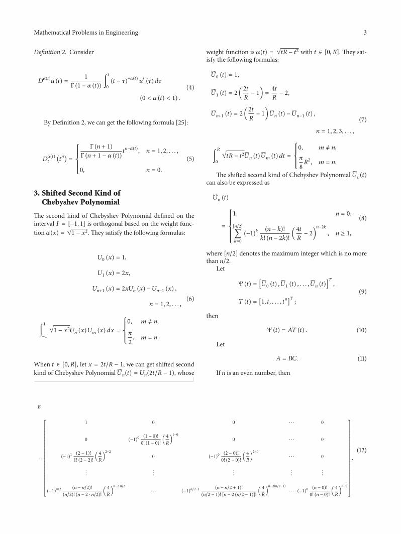
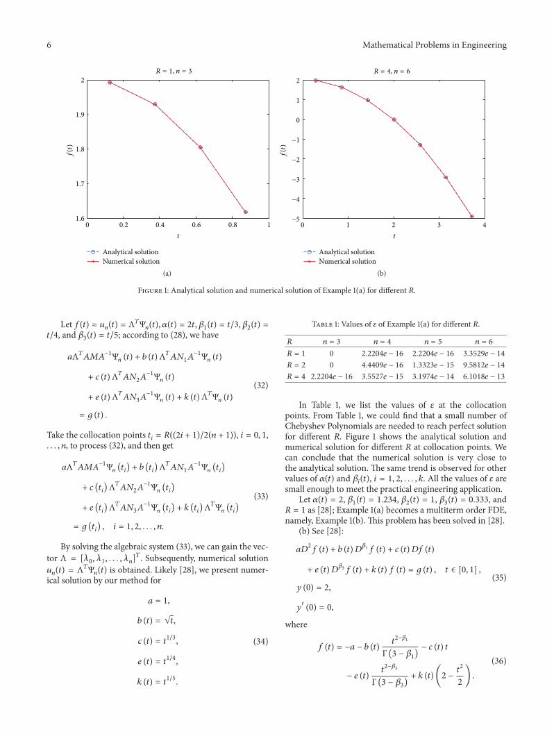
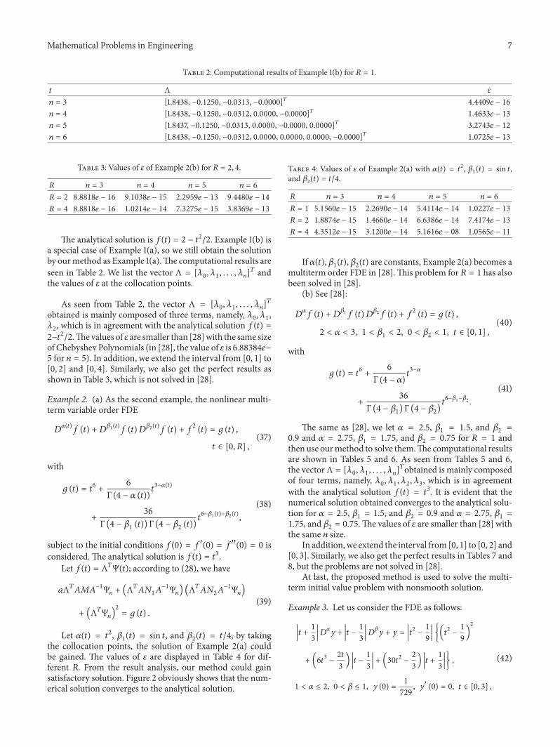
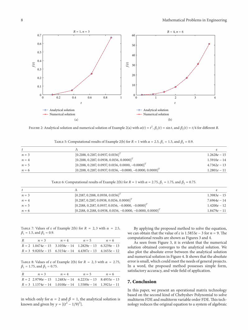
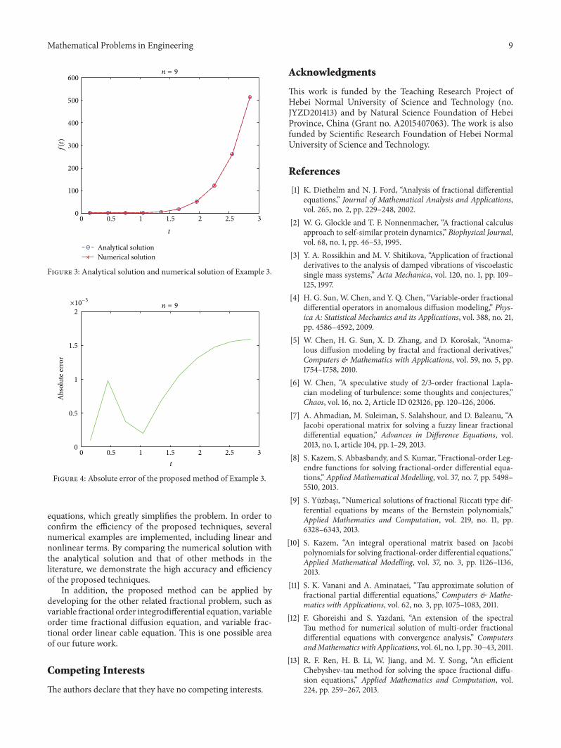


![Fractional Cascading Fractional Cascading I: A Data Structuring Technique Fractional Cascading II: Applications [Chazaelle & Guibas 1986] Dynamic Fractional](https://img.pdfslide.us/doc/110x75/56649ea25503460f94ba64dd/fractional-cascading-fractional-cascading-i-a-data-structuring-technique-fractional.jpg)


![Research Article Design of Fuzzy Fractional PD + I ...downloads.hindawi.com/journals/mpe/2014/676121.pdfin the application of fuzzy PID control [ ]. e fuzzy method o ers a systematic](https://img.pdfslide.us/doc/110x75/5e7dc2e78d31ab77706606b8/research-article-design-of-fuzzy-fractional-pd-i-in-the-application-of-fuzzy.jpg)


![Research Article A New Biobjective Model to …downloads.hindawi.com/journals/mpe/2015/396864.pdfwith preventive maintenance scheduling problem have been done by [ ] during the last](https://img.pdfslide.us/doc/110x75/5f339bce25fcbd3dfd792d39/research-article-a-new-biobjective-model-to-with-preventive-maintenance-scheduling.jpg)