Research Article An Improved Approach for Estimating the

Research ArticleAn Improved Approach for Estimating the Hyperparameters ofthe Kriging Model for High-Dimensional Problems through thePartial Least Squares Method

Mohamed Amine Bouhlel1 Nathalie Bartoli2 Abdelkader Otsmane3 and Joseph Morlier4

1Department of Aerospace Engineering University of Michigan 1320 Beal Avenue Ann Arbor MI 48109 USA2ONERA 2 Avenue Edouard Belin 31055 Toulouse France3SNECMA Rond-Point Rene Ravaud-Reau 77550 Moissy-Cramayel France4Institut Clement Ader CNRS ISAE-SUPAERO Universite de Toulouse 10 Avenue Edouard Belin 31055 Toulouse Cedex 4 France

Correspondence should be addressed to Mohamed Amine Bouhlel bouhlelmohamedaminegmailcom

Received 31 December 2015 Revised 10 May 2016 Accepted 24 May 2016

Academic Editor Erik Cuevas

Copyright copy 2016 Mohamed Amine Bouhlel et al This is an open access article distributed under the Creative CommonsAttribution License which permits unrestricted use distribution and reproduction in any medium provided the original work isproperly cited

During the last years kriging has become one of the most popular methods in computer simulation andmachine learning Krigingmodels have been successfully used in many engineering applications to approximate expensive simulation models When manyinput variables are used kriging is inefficient mainly due to an exorbitant computational time required during its construction Tohandle high-dimensional problems (100+) one method is recently proposed that combines kriging with the Partial Least Squarestechnique the so-called KPLS model This method has shown interesting results in terms of saving CPU time required to buildmodel while maintaining sufficient accuracy on both academic and industrial problems However KPLS has provided a pooraccuracy compared to conventional kriging on multimodal functions To handle this issue this paper proposes adding a new stepduring the construction of KPLS to improve its accuracy for multimodal functions When the exponential covariance functionsare used this step is based on simple identification between the covariance function of KPLS and kriging The developed methodis validated especially by using a multimodal academic function known as Griewank function in the literature and we show thegain in terms of accuracy and computer time by comparing with KPLS and kriging

1 Introduction

During the last years the kriging model [1ndash4] which isreferred to as the Gaussian process model [5] has becomeone of the most popular methods in computer simulationand machine learning It is used as a substitute of high-fidelity codes representing physical phenomena and aims toreduce the computational time of a particular process Forinstance the kriging model is used successfully in severaloptimization problems [6ndash11] Kriging is not well adapted tohigh-dimensional problem principally due to large matrixinversion problems In fact the krigingmodel becomesmuchtime consuming when a large number of input variables areused since a large number of sampling points are required

Indeed it is recommended in [12] to use 10119889 samplingpoints with 119889 the number of dimensions for obtaining agood accuracy of the kriging model As a result we needto increase the size of the kriging covariance matrix whichbecomes computationally very expensive to invertMoreoverthis inversionrsquos problem induces difficulty in the classicalhyperparameters estimation through themaximization of thelikelihood function

A recentmethod called KPLS [13] is developed to reducecomputational time which uses during a construction of thekriging model the dimensional reduction method ldquoPartialLeast Squaresrdquo (PLS) This method is able to reduce thenumber of hyperparameters of a kriging model such thattheir number becomes equal to the number of principal

Hindawi Publishing CorporationMathematical Problems in EngineeringVolume 2016 Article ID 6723410 11 pageshttpdxdoiorg10115520166723410

2 Mathematical Problems in Engineering

components retained by the PLS method The KPLS methodis thus able to rapidly build a kriging model for high-dimensional problems (100+) while maintaining a goodaccuracy However it has been shown in [13] that the KPLSmodel is less accurate than the kriging model in many casesin particular for multimodal functions

In this paper we propose an extra step that supplements[13] in order to improve its accuracy Under hypothesis thatkernels used for building the KPLS model are of exponentialtype with the same form (all Gaussian kernels eg) wechoose the hyperparameters found by the KPLS model asan initial point to optimize the likelihood function of aconventional kriging model In fact this approach is per-formed by identifying the covariance function of the KPLSmodel as a covariance function of a kriging model The factof considering the identified kriging model instead of theKPLS model leads to extending the search space where thehyperparameters are defined and thus tomaking the resultingmodel more flexible than the KPLS model

This paper is organized in 3 main sections In Section 2we present a review of the KPLS model In Section 3 wediscuss our new approach under the hypothesis needed for itsapplicability Finally numerical results are shown to confirmthe efficiency of our method followed by a summary of whatwe have achieved

2 Construction of KPLS

In this section we introduce the notation and describe thetheory behind the construction of the KPLS model Assumethat we have evaluated a cost deterministic function of 119899points x(119894) (119894 = 1 119899) with x(119894) = [119909(119894)1 119909

(119894)

119889] isin 119861 sub

R119889 and we denote X by the matrix [x(1)119905 x(119899)119905]119905 Forsimplicity 119861 is considered to be a hypercube expressed bythe product between intervals of each direction space thatis 119861 = prod

119889

119895=1[119886119895 119887119895] where 119886119895 119887119895 isin R with 119886119895 le 119887119895 for119895 = 1 119889 Simulating these 119899 inputs gives the outputsy = [119910(1) 119910(119899)]119905 with 119910(119894) = 119910(x(119894)) for 119894 = 1 119899

21 Construction of the Kriging Model For building thekriging model we assume that the deterministic response119910(x) is realization of a stochastic process [14ndash17]

119884 (x) = 1205730 + 119885 (x) (1)

The presented formula with 1205730 an unknown constant corre-sponds to ordinary kriging [8] which is a particular case ofuniversal kriging [15]The stochastic term119885(x) is consideredas realization of a stationaryGaussian process withE[119885(x)] =0 and a covariance function also called kernel function givenby

Cov (119885 (x) 119885 (x1015840)) = 119896 (x x1015840) = 1205902119903 (x x1015840) = 1205902119903xx1015840

forallx x1015840 isin 119861(2)

where 1205902 is the process variance and 119903xx1015840 is the correlationfunction between x and x1015840 However the correlation function

119903 depends on hyperparameters 120579 which are considered tobe known We also denote the 119899 times 1 vector as rxX =

[119903xx(1) 119903xx(119899)]119905 and the 119899 times 119899 correlation matrix as R =

[rx(1)X rx(119899)X] We use (x) to denote the prediction ofthe true function 119910(x) Under the hypothesis above the bestlinear unbiased predictor for 119910(x) given the observations yis

(x) = 1205730 + r119905

xXRminus1(y minus 12057301) (3)

where 1 denotes an 119899-vector of ones and

1205730 = (1119905Rminus11)

minus11119905Rminus1y (4)

In addition the estimation of 1205902 is given by

2=1

119899(y minus 11205730)

119905Rminus1 (y minus 11205730) (5)

Moreover ordinary kriging provides an estimate of thevariance of the prediction which is given by

1199042(x) = 2 (1 minus r119905xXR

minus1rxX) (6)

Note that the assumption of a known covariance functionwith known parameters 120579 is unrealistic in reality and theyare often unknown For this reason the covariance func-tion is typically chosen from among a parametric familyof kernels In this work only the covariance functions ofexponential type are considered in particular the Gaussiankernel Indeed theGaussian kernel is themost popular kernelin kriging metamodels of simulation models which is givenby

119896 (x x1015840) = 1205902119889

prod

119894=1

exp (minus120579119894 (119909119894 minus 1199091015840

119894)2) forall120579119894 isin R

+ (7)

We note that the parameters 120579119894 for 119894 = 1 119889 can beinterpreted as measuring how strongly the input variables1199091 119909119889 respectively affect the output 119910 If 120579119894 is very largethe kernel 119896(x x1015840) given by (7) tends to zero and thus leads to alow correlation In fact we see in Figure 1 how the correlationcurve rapidly varies from a point to another when 120579 = 10

However the estimator of the kriging parameters (1205730 2

and 1205791 120579119889) makes the kriging predictor given by (3)nonlinear and makes the estimated predictor variance givenby (6) biased We note that the vector r and the matrix Rshould get hats above but it is ignored in practice [18]

22 Partial Least Squares The PLS method is a statisti-cal method which searches out the best multidimensionaldirection X that explains the characteristics of the outputy It finds a linear relationship between input variables andoutput variable by projecting input variables onto principalcomponents also called latent variables The PLS techniquereduces dimension and reveals how inputs depend on outputIn the following we use ℎ to denote the number of principalcomponents retained which are a lot lower than 119889 (ℎ ≪119889) ℎ does not generally exceed 4 in practice In addition

Mathematical Problems in Engineering 3

120579 = 1

120579 = 10

eminus|x

(119894) minus

x(119895) |2

00

02

04

06

08

10

05 10 15 20 25 3000|x(i) minus x(j)|

Figure 1 Theta smoothness can be tuned to adapt spatial influenceto our problemThemagnitude of 120579 dictates howquickly the squaredexponential function variates

the principal components can be computed sequentiallyIn fact the principal component t(119897) for 119897 = 1 ℎ iscomputed by seeking the best directionw(119897) whichmaximizesthe squared covariance between t(119897) = X(119897minus1)w(119897) and y(119897minus1)

w(119897) =

argmaxw(119897)

w(119897)119905X(119897minus1)119905y(119897minus1)y(119897minus1)119905X(119897minus1)w(119897)

such that w(119897)119905w(119897) = 1(8)

where X = X(0) y = y(0) and for 119897 = 1 ℎ X(119897) and y(119897) arethe residualmatrix from the local regression ofX(119897minus1) onto theprincipal component t(119897) and from the local regression of y(119897)

onto the principal component t(119897) respectively such that

X(119897) = X(119897minus1) minus t(119897)p(119897)

y(119897) = y(119897minus1) minus 119888119897t(119897)

(9)

where p(119897) (a 1 times 119889 vector) and 119888119897 (a coefficient) contain theregression coefficients For more details of how PLS methodworks please see [19ndash21]

The principal components represent the new coordinatesystem obtained upon rotating the original system with axes1199091 119909119889 [21] For 119897 = 1 ℎ t(119897) can be written as

t(119897) = X(119897minus1)w(119897) = Xw(119897)lowast (10)

This important relationship is mainly used for developing theKPLSmodel which is detailed in Section 23The vectorsw(119897)lowast for 119897 = 1 ℎ are given by the following matrix Wlowast =[w(1)lowast w

(ℎ)lowast ] which is obtained by (for more details see

[22])

Wlowast =W (P119905W)minus1 (11)

whereW = [w(1) w(ℎ)] and P = [p(1)119905 p(ℎ)119905]

Table 1 Results for tab1 experiment data (24 input variables outputvariables 1199103) obtained by using 99 training points 52 validationpoints and the error given by (18) ldquoKrigingrdquo refers to the ordinarykriging Optimus solution and ldquoKPLSℎrdquo and ldquoKPLSℎ+Krdquo refer toKPLS and KPLS+K with ℎ principal components respectively Bestresults of the relative error are highlighted in bold type

Surrogate model RE () CPU time

tab1

Kriging 897 817 sKPLS1 1035 018 sKPLS2 1033 042 sKPLS3 1041 114 s

KPLS1+K 877 215 sKPLS2+K 872 422 sKPLS3+K 873 453 s

23 Construction of the KPLS Model The hyperparameters120579 = 120579119894 for 119894 = 1 119889 given by (7) are found by maxi-mum likelihood estimation (MLE) methodTheir estimationbecomes more and more expensive when 119889 increases Thevector 120579 can be interpreted as measuring how stronglythe variables 1199091 119909119889 affect the output 119910 respectivelyFor building KPLS coefficients given by vectors w(119897)lowast willbe considered as measuring of the influence of the inputvariables 1199091 119909119889 on the output 119910 By some elementaryoperations on the kernel functions we define theKPLS kernelby

119896KPLS1ℎ (x x1015840) =

ℎ

prod

119897=1

119896119897 (119865119897 (x) 119865119897 (x1015840)) (12)

where 119896119897119861 times 119861 rarr R is an isotropic stationary kernel and

119865119897 119861 997888rarr 119861

x 997891997888rarr [119908(119897)lowast11199091 119908(119897)

lowast119889119909119889]

(13)

More details of such construction are given in [13]Considering the example of the Gaussian kernel given by (7)we obtain

119896 (x x1015840) = 1205902ℎ

prod

119897=1

119889

prod

119894=1

exp [minus120579119897 (119908(119897)

lowast119894119909119894 minus 119908(119897)

lowast1198941199091015840

119894)2]

forall120579119897 isin R+

(14)

Since a small number of principal components are retainedthe estimation of the hyperparameters 1205791 120579ℎ is faster thanthe hyperparameters 1205791 120579119889 given by (7) where 119889 is veryhigh (100+)

3 Transition from the KPLS Model tothe Kriging Model Using the ExponentialCovariance Functions

In this section we show that if all kernels 119896119897 for 119897 = 1 ℎused in (12) are of the exponential type with the same form(all Gaussian kernels eg) then the kernel 119896KPLS1ℎ given by(12) will be of the exponential type with the same form as 119896119897(Gaussian if all 119896119897 are Gaussian)


Table 2 Results of the Griewank function in 20D over the interval [minus5 5] Ten trials are done for each test (50 100 200 and 300 trainingpoints) Best results of the relative error are highlighted in bold type for each case

Surrogate Statistic 50 points 100 pointsError () CPU time Error () CPU time

Kriging Mean 062 3043 s 043 4009 sstd 003 903 s 004 1196 s

KPLS1 Mean 054 005 s 053 012 sstd 003 0007 s 003 002 s



KPLS1+K Mean 059 120 s 045 242 sstd 004 016 s 007 044 s











31 Proof of the Equivalence between the Kernels of the KPLSModel and the Kriging Model Let us define for 119894 = 1 119889120578119894 = sum

ℎ

119897=1 120579119897119908(119897)

lowast119894

2 we have

1198961ℎ (x x1015840) =

ℎ

prod

119897=1

119889

prod

119894=1

exp (minus120579119897119908(119897)

lowast119894

2(119909119894 minus 119909

1015840

119894)2)

= exp(119889

sum

119894=1

ℎ

sum

119897=1

minus 120579119897119908(119897)

lowast119894

2(119909119894 minus 119909

1015840

119894)2)

= exp(119889

sum

119894=1

minus 120578119894 (119909119894 minus 1199091015840

119894)2)

=

119889

prod

119894=1

exp (minus120578119894 (119909119894 minus 1199091015840

119894)2)

(15)

In the same way we can show this equivalence for the otherexponential kernels where 1199011 = sdot sdot sdot = 119901ℎ

1198961ℎ (x x1015840) = 1205902ℎ

prod

119897=1

119889

prod

119894=1

exp (minus12057911989710038161003816100381610038161003816119908(119897)

lowast119894 (119909119894 minus 1199091015840

119894)10038161003816100381610038161003816

119901119897

) (16)

However we must caution that the above proof showsequivalence between the covariance functions of KPLS andkriging only on a subspace domain More precisely theKPLS covariance function is defined in a subspace from R+

119889

whereas the kriging covariance function is defined in thecomplete R+

119889 domain Thus our original idea is to extendthe space where the KPLS covariance function is defined forthe complete space R+119889

32 A New Step during the Construction of the KPLS ModelKPLS+K By considering the equivalence shown in the last



















section we propose to add a new step during the con-struction of the KPLS model This step occurs just afterthe 120579119897-estimation for 119897 = 1 ℎ It involves making localoptimization of the likelihood function of the kriging modelequivalent to the KPLS model Moreover we use 120578119894 =sumℎ

119897=1 120579119897119908(119897)

lowast119894

2 for 119894 = 1 119889 as a starting point of the local

optimization by considering the solution 120579119897 for 119897 = 1 ℎfound by the KPLS method Thus this optimization is donein the complete space where the vector 120578 = 120578119894 isin R

+119889This approach called KPLS+K aims to improve the MLE

of the kriging model equivalent to the associated KPLSmodel In fact the local optimization of the equivalentkriging offers more possibilities for improving the MLEby considering a wider search space and thus it will beable to correct the estimation of many directions Thesedirections are represented by 120578119894 for the 119894th direction which isbadly estimated by the KPLSmethod Because estimating theequivalent kriging hyperparameters can be time consuming

especially when 119889 is large we improve the MLE by a localoptimization at the cost of a slight increase of computationaltime

Figure 2 recalls the principal stages of building a KPLS+Kmodel

4 Numerical Simulations

We now focus on the performance of KPLS+K by comparingit with the KPLS model and the ordinary kriging modelFor this purpose we use the academic function namedGriewank over the interval [minus5 5] which is studied in [13]20 and 60 dimensions are considered for this function Inaddition an engineering example done at Snecma for amultidisciplinary optimization is usedThis engineering caseis chosen since it was shown in [13] that KPLS is less accuratethan ordinary kriging The Gaussian kernel is used for allsurrogatemodels used herein that is ordinary kriging KPLSand KPLS+K For KPLS and KPLS+K using ℎ principal


(1) To choose an exponential kernel function

(2) To define the covariance functiongiven by (12)

for i = 1 d by using the starting(4) To optimize locally the parameters 120578i

(3) To estimate the parameters120579l for l = 1 h

point 120578i = lw(l)2

lowasti (Gaussian example)sumh

l=1120579

Figure 2 Principal stages for building a KPLS+K model

minus2

minus4

0

00

05

10

20

15

24

minus2minus4

02

4

Figure 3 A 2D Griewank function over the interval [minus5 5]

components for ℎ le 119889 will be denoted by KPLSℎ andKPLSℎ+K respectively and this ℎ is varied from 1 to 3 ThePython toolbox Scikit-learn v014 [23] is used to achieve theproposed numerical tests except for ordinary kriging used onthe industrial case where the Optimus version is used Thetraining and the validation points used in [13] are reused inthe following

41 Griewank Function over the Interval [minus5 5] The Grie-wank function [13 24] is defined by

119910Griewank (x) =119889

sum

119894=1

1199092119894

4000minus

119889

prod

119894=1

cos(119909119894

radic119894

) + 1

minus5 le 119909119894 le 5 for 119894 = 1 119889

(17)

Figure 3 shows the degree of complexity of such functionwhich is very multimodal As in [13] we consider 119889 = 20 and119889 = 60 input variables For each problem ten experimentsbased on the random Latin-hypercube design are built with119899 (number of sampling points) equal to 50 100 200 and 300

To better visualize the results boxplots are used to show theCPU time and the relative error RE given by

Error =10038171003817100381710038171003817Y minus Y100381710038171003817100381710038172Y2

100 (18)

where sdot 2 represents the usual 1198712 norm and Y and Yare the vectors containing the prediction and the real valuesof 5000 randomly selected validation points for each caseThe mean and the standard error are given in Tables 2 and3 respectively in Appendix However the results of theordinary kriging model and the KPLS model are reportedfrom [13]

For 20 input variables and 50 sampling points theKPLS models always give a more accurate solution thanordinary kriging and KPLS+K as shown in Figure 4(a)Indeed the best result is given by KPLS3 with a mean ofRE equal to 051 However the KPLS+K models give moreaccurate models than ordinary kriging in this case (058 forKPLS2+K and KPLS3+K versus 062 for ordinary kriging)For the KPLS model the rate of improvement with respectto the number of sampling points is less than for ordinarykriging and KPLS+K (see Figures 4(b)ndash4(d)) As a resultKPLSℎ+K for ℎ = 1 3 and ordinary kriging give almostthe same accuracy (asymp016) when 300 sampling points areused (as shown in Figure 4(d)) whereas theKPLSmodels givea RE of 035 as a best result when ℎ = 3

Nevertheless the results shown in Figure 5 indicate thatthe KPLS+K models lead to an important reduction in CPUtime for the various number of sampling points compared toordinary kriging For instance 2049 s are required for build-ing KPLS3+K when 300 training points are used whereasordinary kriging is built in 9431 s in this case KPLS3+Kis thus approximately 4 times cheaper than the ordinarykriging model Moreover the computational time requiredfor building KPLS+K is more stable than the computationaltime for building ordinary kriging standard deviations ofapproximately 3 s for KPLS+K and 22 s for the ordinarykriging model are observed

For 60 input variables and 50 sampling points a slightdifference of the results occurs compared to the 20 inputvariables case (Figure 6(a)) Indeed the KPLSmodels remainalways better with a mean of RE approximately equal to092 than KPLS+K and ordinary kriging However theKPLS+K models give more accurate results than ordinarykriging with an accuracy close to that of KPLS (asymp099versus 139) Increasing the number of sampling pointsthe accuracy of ordinary kriging becomes better than theaccuracy given by the KPLS models but it remains lessaccurate than for the KPLSℎ+K models for ℎ = 2 or 3 Forinstance we obtain a mean of RE with 060 for KPLS2+Kagainst 065 for ordinary kriging (see Figure 6(d)) when300 sampling points are used

As we can observe from Figure 7(d) a very importantreduction in terms of computational time is obtained Indeeda mean time of 289456 s is required for building ordinarykriging whereas KPLS2+K is built in 2303 s KPLS2+K isapproximately 125 times cheaper than ordinary kriging inthis case In addition the computational time for building


KPLS

1

KPLS

2

KPLS

3

Ord

inar

y kr

igin

g

KPLS

1+

K

KPLS

2+

K

KPLS

3+

K

045

050

055

060

065

070RE

(a) RE () for 20 input variables and 50 sampling points

KPLS

1

KPLS

2

KPLS

3

Ord

inar

y kr

igin

g

KPLS

1+

K

KPLS

2+

K

KPLS

3+

K

030

035

040

045

050

055

060

RE(b) RE () for 20 input variables and 100 sampling points

KPLS

1

KPLS

2

KPLS

3

Ord

inar

y kr

igin

g

KPLS

1+

K

KPLS

2+

K

KPLS

3+

K

01

02

03

04

05

RE

(c) RE () for 20 input variables and 200 sampling points

KPLS

1

KPLS

2

KPLS

3

Ord

inar

y kr

igin

g

KPLS

1+

K

KPLS

2+

K

KPLS

3+

K

01

02

03

04

05

RE

(d) RE () for 20 input variables and 300 sampling points

Figure 4 RE of the Griewank function in 20D over the interval [minus5 5] The experiments are based on the 10-Latin-hypercube design

KPLS+K is more stable than ordinary kriging except theKPLS3+K case a standard deviation of approximately 030 sfor KPLS1+K and KPLS2+K is observed against 72848 sfor ordinary kriging However the relatively large standardof deviation of KPLS3+K (2659 s) is probably due to thedispersion caused by KPLS3 (2659 s) But it remains toolower than the standard deviation of the ordinary krigingmodel

For the Griewank function over the interval [minus5 5] theKPLS+K models are slightly more time consuming than theKPLS models but they are more accurate in particular whenthe number of observations is greater than the dimension 119889as is implied by the rule-of-thumb 119899 = 10119889 in [12]They seem

to performwell compared to the ordinary krigingmodel withan important gain in terms of saving CPU time

42 Engineering Case In this section let us consider the thirdoutput 1199103 from tab1 problem studied in [13] This test caseis chosen because the KPLS models from 1 to 3 principalcomponents do not perform well (see Table 1) We recall thatthis problem contains 24 input variables 99 training pointsand 52 validation points are used and the relative error (RE)given by (18) is considered

As we see in Table 1 we improve the accuracy of KPLSby adding the step for building KPLS+K This improvementis verified whatever the number of principal components


KPLS

1

KPLS

2

KPLS

3

Ord

inar

y kr

igin

g

KPLS

1+

K

KPLS

2+

K

KPLS

3+

K

0

10

20

30

40

50Ti

me

(a) CPU time for 20 input variables and 50 sampling points

KPLS

1

KPLS

2

KPLS

3

Ord

inar

y kr

igin

g

KPLS

1+

K

KPLS

2+

K

KPLS

3+

K

0

10

20

30

40

50

60

Tim

e(b) CPU time for 20 input variables and 100 sampling points

KPLS

1

KPLS

2

KPLS

3

Ord

inar

y kr

igin

g

KPLS

1+

K

KPLS

2+

K

KPLS

3+

K

0

20

40

60

80

100

120

140

160

180

Tim

e

(c) CPU time for 20 input variables and 200 sampling points

KPLS

1

KPLS

2

KPLS

3

Ord

inar

y kr

igin

g

KPLS

1+

K

KPLS

2+

K

KPLS

3+

K

0

20

40

60

80

100

120

140Ti

me

(d) CPU time for 20 input variables and 300 sampling points

Figure 5 CPU time of the Griewank function in 20D over the interval [minus5 5] The experiments are based on the 10-Latin-hypercube design

used (1 2 and 3 principal components) For these threemodels a better accuracy is even found than the ordinarykriging model The computational time required to buildKPLS+k is approximately twice lower than the time requiredfor ordinary kriging

5 Conclusions

Motivated by the need to accurately approximate high-fidelitycodes rapidly we develop a new technique for building thekriging model faster than classical techniques used in litera-ture The key idea for such construction relies on the choiceof the start point for optimizing the likelihood function of

the kriging model For this purpose we firstly prove equiva-lence betweenKPLS and kriging when an exponential covari-ance function is used After optimizing hyperparameters ofKPLS we then choose the solution obtained as an initialpoint to find the MLE of the equivalent kriging modelThis approach will be applicable only if the kernels used forbuilding KPLS are of the exponential type with the sameform

The performance of KPLS+K is verified in the Griewankfunction over the interval [minus5 5] with 20 and 60 dimensionsand an industrial case from Snecma where the KPLS modelsdo not perform well in terms of accuracy The results ofKPLS+K have shown a significant improvement in terms of


KPLS

1

KPLS

2

KPLS

3

Ord

inar

y kr

igin

g

RE

08

10

12

14

16

18

KPLS

1+

K

KPLS

2+

K

KPLS

3+

K


KPLS

1

KPLS

2

KPLS

3

Ord

inar

y kr

igin

g

RE

080

085

090

095

100

105

110

115

KPLS

1+

K

KPLS

2+

K

KPLS

3+

K

(b) RE () for 60 input variables and 100 sampling points

KPLS

1

KPLS

2

KPLS

3

Ord

inar

y kr

igin

g

RE

065

070

075

080

085

090

KPLS

1+

K

KPLS

2+

K

KPLS

3+

K


KPLS

1

KPLS

2

KPLS

3

Ord

inar

y kr

igin

g

RE

055

060

065

070

075

080

085

KPLS

1+

K

KPLS

2+

K

KPLS

3+

K



accuracy compared to the results of KPLS at the cost of aslight increase in computational time We have also seenin some cases that accuracy of KPLS+K is even better thanaccuracy given by the ordinary kriging model

Appendix

Results of Griewank Function in 20D and 60Dover the Interval [minus5 5]

In Tables 2 and 3 the mean and the standard deviation (std)of the numerical experiments with theGriewank function aregiven for 20 and 60 dimensions respectively

Symbols and Notation (Matrices and VectorsAre in Bold Type)

| sdot | Absolute valueR Set of real numbersR+ Set of positive real numbers119899 Number of sampling points119889 Dimensionℎ Number of principal components

retainedx A 1 times 119889 vector119909119894 The 119894th element of a vector xX A 119899 times 119889matrix containing sampling

points


KPLS

1

KPLS

2

KPLS

3

Ord

inar

y kr

igin

g

KPLS

1+

K

KPLS

2+

K

KPLS

3+

K

0

100

200

300

400

500

600

700

800

900Ti

me


KPLS

1

KPLS

2

KPLS

3

Ord

inar

y kr

igin

g

KPLS

1+

K

KPLS

2+

K

KPLS

3+

K

0

200

400

600

800

1000

1200

1400

Tim


KPLS

1

KPLS

2

KPLS

3

Ord

inar

y kr

igin

g

KPLS

1+

K

KPLS

2+

K

KPLS

3+

K

0

500

1000

1500

2000

2500

Tim

e


KPLS

1

KPLS

2

KPLS

3

Ord

inar

y kr

igin

g

KPLS

1+

K

KPLS

2+

K

KPLS

3+

K

0

500

1000

1500

2000

2500

3000

3500

4000Ti

me



119910(x) The true function 119910 performed on thevector x

y 119899 times 1 vector containing simulation ofX

(x) The prediction of the true function 119910(x)119884(x) A stochastic processx(119894) The 119894th training point for 119894 = 1 119899 (a

1 times 119889 vector)w(119897) A 119889 times 1 vector containing119883-weights

given by the 119897th PLS-iteration for119897 = 1 ℎ

X(0) X

X(119897minus1) Matrix containing residual of the innerregression of the (119897 minus 1)th PLS-iteration for119897 = 1 ℎ

119896(sdot sdot) A covariance functionx119905 Superscript 119905 denoting the transpose

operation of the vector xasymp Approximately sign

Competing Interests

The authors declare that there is no conflict of interestsregarding the publication of this paper


Acknowledgments

The authors extend their grateful thanks to A Chiplunkarfrom ISAE-SUPAERO Toulouse for his careful correction ofthe paper

References

[1] D Krige ldquoA statistical approach to some basic mine valuationproblems on the Witwatersrandrdquo Journal of the ChemicalMetallurgical and Mining Society vol 52 pp 119ndash139 1951

[2] G Matheron ldquoPrinciples of geostatisticsrdquo Economic Geologyvol 58 no 8 pp 1246ndash1266 1963

[3] N Cressie ldquoSpatial prediction and ordinary krigingrdquo Mathe-matical Geology vol 20 no 4 pp 405ndash421 1988

[4] J Sacks S B Schiller and W J Welch ldquoDesigns for computerexperimentsrdquo Technometrics vol 31 no 1 pp 41ndash47 1989

[5] C E Rasmussen and C K Williams Gaussian Processes forMachine Learning Adaptive Computation and Machine Learn-ing MIT Press Cambridge Mass USA 2006

[6] D R Jones M Schonlau and W J Welch ldquoEfficient globaloptimization of expensive black-box functionsrdquo Journal ofGlobal Optimization vol 13 no 4 pp 455ndash492 1998

[7] S Sakata F Ashida and M Zako ldquoStructural optimizatiionusing Kriging approximationrdquo Computer Methods in AppliedMechanics and Engineering vol 192 no 7-8 pp 923ndash939 2003

[8] A Forrester A Sobester and A Keane Engineering Design viaSurrogateModelling A Practical Guide JohnWileyamp Sons NewYork NY USA 2008

[9] J Laurenceau Kriging based response surfaces for aerodynamicshape optimization [Thesis] Institut National Polytechnique deToulouse (INPT) Toulouse France 2008

[10] J P C Kleijnen W van Beers and I van Nieuwenhuyse ldquoCon-strained optimization in expensive simulation novel approachrdquoEuropean Journal of Operational Research vol 202 no 1 pp164ndash174 2010

[11] J P KleijnenW vanBeers and I vanNieuwenhuyse ldquoExpectedimprovement in efficient global optimization through boot-strapped krigingrdquo Journal of Global Optimization vol 54 no1 pp 59ndash73 2012

[12] J L Loeppky J Sacks and W J Welch ldquoChoosing the samplesize of a computer experiment a practical guiderdquoTechnometricsvol 51 no 4 pp 366ndash376 2009

[13] M A Bouhlel N Bartoli A Otsmane and J Morlier ldquoImprov-ing kriging surrogates of high-dimensional design modelsby partial least squares dimension reductionrdquo Structural andMultidisciplinary Optimization vol 53 no 5 pp 935ndash952 2016

[14] J SacksW JWelch T J Mitchell andH PWynn ldquoDesign andanalysis of computer experimentsrdquo Statistical Science vol 4 no4 pp 409ndash435 1989

[15] M Sasena Flexibility and efficiency enhancements for con-strained global design optimization with Kriging approximations[PhD thesis] University of Michigan 2002

[16] V Picheny D Ginsbourger Y Richet and G Caplin ldquoQuantile-based optimization of noisy computer experimentswith tunableprecisionrdquo Technometrics vol 55 no 1 pp 2ndash13 2013

[17] O Roustant D Ginsbourger and Y Deville ldquoDiceKrigingDiceOptim two R packages for the analysis of computerexperiments by kriging-based metamodeling and optimiza-tionrdquo Journal of Statistical Software vol 51 no 1 pp 1ndash55 2012

[18] J P Kleijnen Design and Analysis of Simulation Experimentsvol 230 Springer Berlin Germany 2015

[19] I S Helland ldquoOn the structure of partial least squares regres-sionrdquo Communications in Statistics Simulation and Computa-tion vol 17 no 2 pp 581ndash607 1988

[20] l E Frank and J H Friedman ldquoA statistical view of somechemometrics regression toolsrdquoTechnometrics vol 35 no 2 pp109ndash135 1993

[21] R A Perez and G Gonzalez-Farias ldquoPartial least squaresregression on symmetric positive-definite matricesrdquo RevistaColombiana de Estadıstica vol 36 no 1 pp 177ndash192 2013

[22] R Manne ldquoAnalysis of two partial-least-squares algorithms formultivariate calibrationrdquo Chemometrics and Intelligent Labora-tory Systems vol 2 no 1ndash3 pp 187ndash197 1987

[23] F Pedregosa G Varoquaux A Gramfort et al ldquoScikit-learnmachine learning in Pythonrdquo Journal of Machine LearningResearch (JMLR) vol 12 pp 2825ndash2830 2011

[24] R G Regis and C A Shoemaker ldquoCombining radial basisfunction surrogates and dynamic coordinate search in high-dimensional expensive black-box optimizationrdquo EngineeringOptimization vol 45 no 5 pp 529ndash555 2013

Submit your manuscripts athttpwwwhindawicom

Hindawi Publishing Corporationhttpwwwhindawicom Volume 2014

MathematicsJournal of


Mathematical Problems in Engineering

Hindawi Publishing Corporationhttpwwwhindawicom

Differential EquationsInternational Journal of

Volume 2014

Applied MathematicsJournal of


Probability and StatisticsHindawi Publishing Corporationhttpwwwhindawicom Volume 2014

Journal of


Mathematical PhysicsAdvances in

Complex AnalysisJournal of


OptimizationJournal of


CombinatoricsHindawi Publishing Corporationhttpwwwhindawicom Volume 2014

International Journal of


Operations ResearchAdvances in

Journal of


Function Spaces

Abstract and Applied AnalysisHindawi Publishing Corporationhttpwwwhindawicom Volume 2014

International Journal of Mathematics and Mathematical Sciences


The Scientific World JournalHindawi Publishing Corporation httpwwwhindawicom Volume 2014


Algebra

Discrete Dynamics in Nature and Society



Decision SciencesAdvances in

Discrete MathematicsJournal of


Volume 2014 Hindawi Publishing Corporationhttpwwwhindawicom Volume 2014

Stochastic AnalysisInternational Journal of


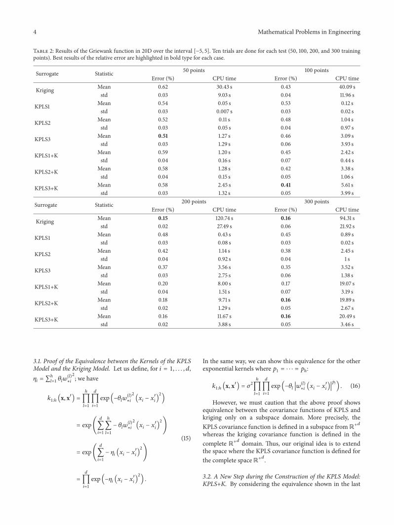
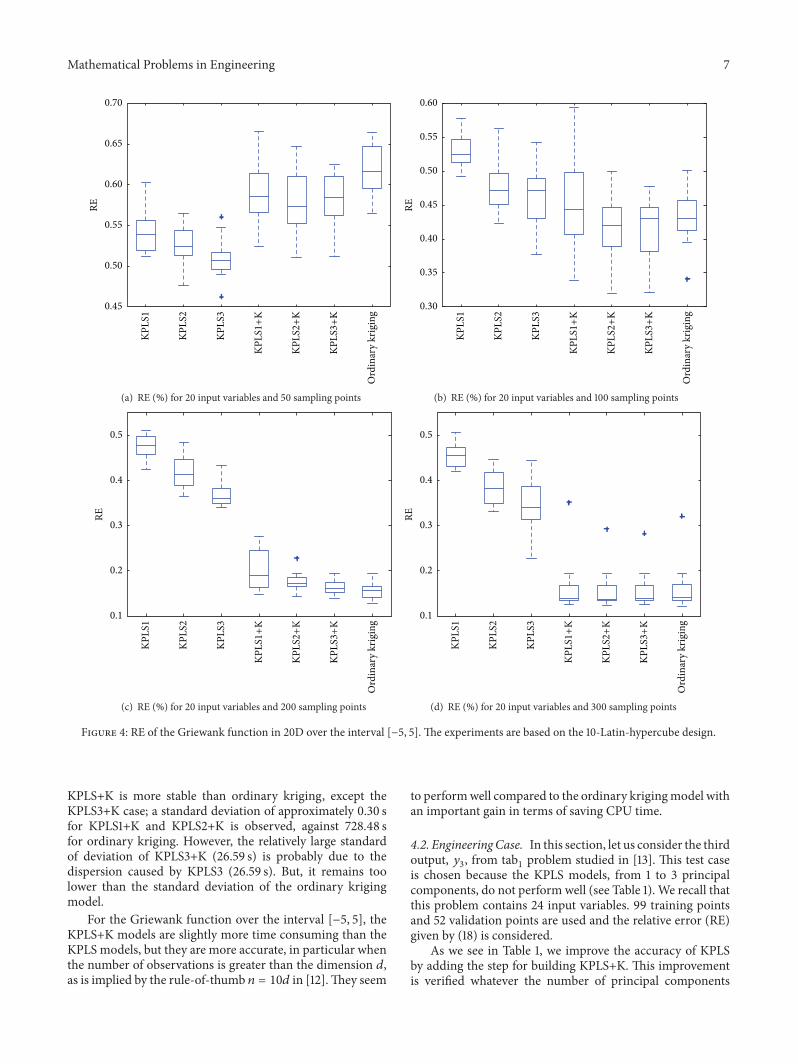
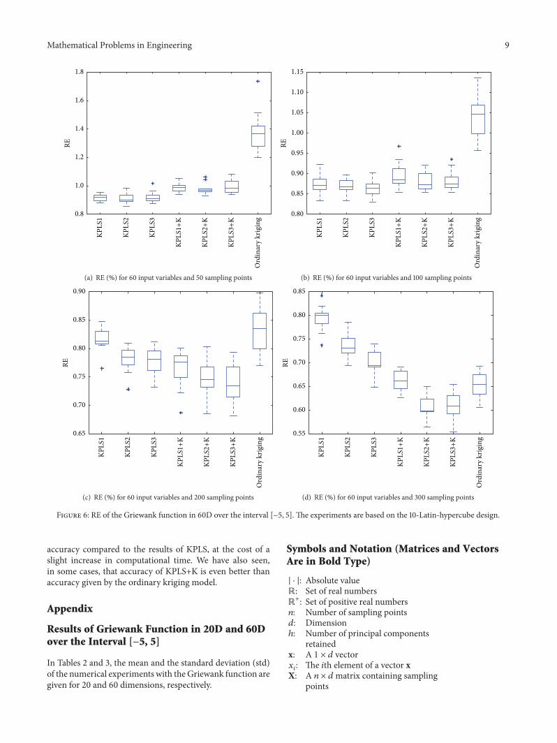
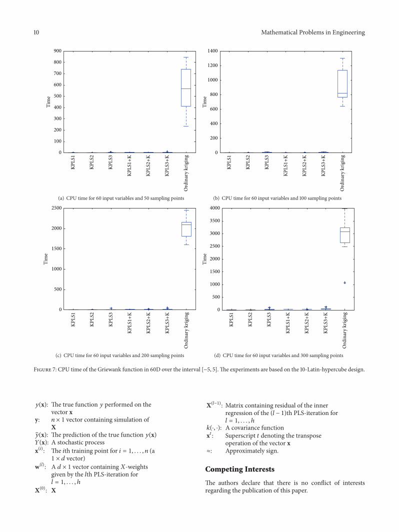components retained by the PLS method The KPLS methodis thus able to rapidly build a kriging model for high-dimensional problems (100+) while maintaining a goodaccuracy However it has been shown in [13] that the KPLSmodel is less accurate than the kriging model in many casesin particular for multimodal functions

In this paper we propose an extra step that supplements[13] in order to improve its accuracy Under hypothesis thatkernels used for building the KPLS model are of exponentialtype with the same form (all Gaussian kernels eg) wechoose the hyperparameters found by the KPLS model asan initial point to optimize the likelihood function of aconventional kriging model In fact this approach is per-formed by identifying the covariance function of the KPLSmodel as a covariance function of a kriging model The factof considering the identified kriging model instead of theKPLS model leads to extending the search space where thehyperparameters are defined and thus tomaking the resultingmodel more flexible than the KPLS model

This paper is organized in 3 main sections In Section 2we present a review of the KPLS model In Section 3 wediscuss our new approach under the hypothesis needed for itsapplicability Finally numerical results are shown to confirmthe efficiency of our method followed by a summary of whatwe have achieved

2 Construction of KPLS

In this section we introduce the notation and describe thetheory behind the construction of the KPLS model Assumethat we have evaluated a cost deterministic function of 119899points x(119894) (119894 = 1 119899) with x(119894) = [119909(119894)1 119909

(119894)

119889] isin 119861 sub

R119889 and we denote X by the matrix [x(1)119905 x(119899)119905]119905 Forsimplicity 119861 is considered to be a hypercube expressed bythe product between intervals of each direction space thatis 119861 = prod

119889

119895=1[119886119895 119887119895] where 119886119895 119887119895 isin R with 119886119895 le 119887119895 for119895 = 1 119889 Simulating these 119899 inputs gives the outputsy = [119910(1) 119910(119899)]119905 with 119910(119894) = 119910(x(119894)) for 119894 = 1 119899

21 Construction of the Kriging Model For building thekriging model we assume that the deterministic response119910(x) is realization of a stochastic process [14ndash17]

119884 (x) = 1205730 + 119885 (x) (1)

The presented formula with 1205730 an unknown constant corre-sponds to ordinary kriging [8] which is a particular case ofuniversal kriging [15]The stochastic term119885(x) is consideredas realization of a stationaryGaussian process withE[119885(x)] =0 and a covariance function also called kernel function givenby

Cov (119885 (x) 119885 (x1015840)) = 119896 (x x1015840) = 1205902119903 (x x1015840) = 1205902119903xx1015840

forallx x1015840 isin 119861(2)

where 1205902 is the process variance and 119903xx1015840 is the correlationfunction between x and x1015840 However the correlation function

119903 depends on hyperparameters 120579 which are considered tobe known We also denote the 119899 times 1 vector as rxX =

[119903xx(1) 119903xx(119899)]119905 and the 119899 times 119899 correlation matrix as R =

[rx(1)X rx(119899)X] We use (x) to denote the prediction ofthe true function 119910(x) Under the hypothesis above the bestlinear unbiased predictor for 119910(x) given the observations yis

(x) = 1205730 + r119905

xXRminus1(y minus 12057301) (3)

where 1 denotes an 119899-vector of ones and

1205730 = (1119905Rminus11)

minus11119905Rminus1y (4)

In addition the estimation of 1205902 is given by

2=1

119899(y minus 11205730)

119905Rminus1 (y minus 11205730) (5)

Moreover ordinary kriging provides an estimate of thevariance of the prediction which is given by

1199042(x) = 2 (1 minus r119905xXR

minus1rxX) (6)

Note that the assumption of a known covariance functionwith known parameters 120579 is unrealistic in reality and theyare often unknown For this reason the covariance func-tion is typically chosen from among a parametric familyof kernels In this work only the covariance functions ofexponential type are considered in particular the Gaussiankernel Indeed theGaussian kernel is themost popular kernelin kriging metamodels of simulation models which is givenby

119896 (x x1015840) = 1205902119889

prod

119894=1

exp (minus120579119894 (119909119894 minus 1199091015840

119894)2) forall120579119894 isin R

+ (7)

We note that the parameters 120579119894 for 119894 = 1 119889 can beinterpreted as measuring how strongly the input variables1199091 119909119889 respectively affect the output 119910 If 120579119894 is very largethe kernel 119896(x x1015840) given by (7) tends to zero and thus leads to alow correlation In fact we see in Figure 1 how the correlationcurve rapidly varies from a point to another when 120579 = 10

However the estimator of the kriging parameters (1205730 2

and 1205791 120579119889) makes the kriging predictor given by (3)nonlinear and makes the estimated predictor variance givenby (6) biased We note that the vector r and the matrix Rshould get hats above but it is ignored in practice [18]

22 Partial Least Squares The PLS method is a statisti-cal method which searches out the best multidimensionaldirection X that explains the characteristics of the outputy It finds a linear relationship between input variables andoutput variable by projecting input variables onto principalcomponents also called latent variables The PLS techniquereduces dimension and reveals how inputs depend on outputIn the following we use ℎ to denote the number of principalcomponents retained which are a lot lower than 119889 (ℎ ≪119889) ℎ does not generally exceed 4 in practice In addition


120579 = 1

120579 = 10

eminus|x

(119894) minus

x(119895) |2

00

02

04

06

08

10

05 10 15 20 25 3000|x(i) minus x(j)|



w(119897) =

argmaxw(119897)


such that w(119897)119905w(119897) = 1(8)



X(119897) = X(119897minus1) minus t(119897)p(119897)

y(119897) = y(119897minus1) minus 119888119897t(119897)

(9)






[22])





tab1




119896KPLS1ℎ (x x1015840) =

ℎ

prod

119897=1

119896119897 (119865119897 (x) 119865119897 (x1015840)) (12)


119865119897 119861 997888rarr 119861

x 997891997888rarr [119908(119897)lowast11199091 119908(119897)

lowast119889119909119889]

(13)


119896 (x x1015840) = 1205902ℎ

prod

119897=1

119889

prod

119894=1

exp [minus120579119897 (119908(119897)

lowast119894119909119894 minus 119908(119897)

lowast1198941199091015840

119894)2]


(14)























ℎ

119897=1 120579119897119908(119897)

lowast119894

2 we have

1198961ℎ (x x1015840) =

ℎ

prod

119897=1

119889

prod

119894=1

exp (minus120579119897119908(119897)

lowast119894

2(119909119894 minus 119909

1015840

119894)2)

= exp(119889

sum

119894=1

ℎ

sum

119897=1

minus 120579119897119908(119897)

lowast119894

2(119909119894 minus 119909

1015840

119894)2)

= exp(119889

sum

119894=1

minus 120578119894 (119909119894 minus 1199091015840

119894)2)

=

119889

prod

119894=1

exp (minus120578119894 (119909119894 minus 1199091015840

119894)2)

(15)


1198961ℎ (x x1015840) = 1205902ℎ

prod

119897=1

119889

prod

119894=1

exp (minus12057911989710038161003816100381610038161003816119908(119897)

lowast119894 (119909119894 minus 1199091015840

119894)10038161003816100381610038161003816

119901119897

) (16)


119889























119897=1 120579119897119908(119897)

lowast119894
















l=1120579


minus2

minus4

0

00

05

10

20

15

24

minus2minus4

02

4




119910Griewank (x) =119889

sum

119894=1

1199092119894

4000minus

119889

prod

119894=1

cos(119909119894

radic119894

) + 1

minus5 le 119909119894 le 5 for 119894 = 1 119889

(17)



Error =10038171003817100381710038171003817Y minus Y100381710038171003817100381710038172Y2

100 (18)







KPLS

1

KPLS

2

KPLS

3

Ord

inar

y kr

igin

g

KPLS

1+

K

KPLS

2+

K

KPLS

3+

K

045

050

055

060

065

070RE


KPLS

1

KPLS

2

KPLS

3

Ord

inar

y kr

igin

g

KPLS

1+

K

KPLS

2+

K

KPLS

3+

K

030

035

040

045

050

055

060


KPLS

1

KPLS

2

KPLS

3

Ord

inar

y kr

igin

g

KPLS

1+

K

KPLS

2+

K

KPLS

3+

K

01

02

03

04

05

RE


KPLS

1

KPLS

2

KPLS

3

Ord

inar

y kr

igin

g

KPLS

1+

K

KPLS

2+

K

KPLS

3+

K

01

02

03

04

05

RE









KPLS

1

KPLS

2

KPLS

3

Ord

inar

y kr

igin

g

KPLS

1+

K

KPLS

2+

K

KPLS

3+

K

0

10

20

30

40

50Ti

me


KPLS

1

KPLS

2

KPLS

3

Ord

inar

y kr

igin

g

KPLS

1+

K

KPLS

2+

K

KPLS

3+

K

0

10

20

30

40

50

60

Tim


KPLS

1

KPLS

2

KPLS

3

Ord

inar

y kr

igin

g

KPLS

1+

K

KPLS

2+

K

KPLS

3+

K

0

20

40

60

80

100

120

140

160

180

Tim

e


KPLS

1

KPLS

2

KPLS

3

Ord

inar

y kr

igin

g

KPLS

1+

K

KPLS

2+

K

KPLS

3+

K

0

20

40

60

80

100

120

140Ti

me




5 Conclusions





KPLS

1

KPLS

2

KPLS

3

Ord

inar

y kr

igin

g

RE

08

10

12

14

16

18

KPLS

1+

K

KPLS

2+

K

KPLS

3+

K


KPLS

1

KPLS

2

KPLS

3

Ord

inar

y kr

igin

g

RE

080

085

090

095

100

105

110

115

KPLS

1+

K

KPLS

2+

K

KPLS

3+

K


KPLS

1

KPLS

2

KPLS

3

Ord

inar

y kr

igin

g

RE

065

070

075

080

085

090

KPLS

1+

K

KPLS

2+

K

KPLS

3+

K


KPLS

1

KPLS

2

KPLS

3

Ord

inar

y kr

igin

g

RE

055

060

065

070

075

080

085

KPLS

1+

K

KPLS

2+

K

KPLS

3+

K




Appendix






points


KPLS

1

KPLS

2

KPLS

3

Ord

inar

y kr

igin

g

KPLS

1+

K

KPLS

2+

K

KPLS

3+

K

0

100

200

300

400

500

600

700

800

900Ti

me


KPLS

1

KPLS

2

KPLS

3

Ord

inar

y kr

igin

g

KPLS

1+

K

KPLS

2+

K

KPLS

3+

K

0

200

400

600

800

1000

1200

1400

Tim


KPLS

1

KPLS

2

KPLS

3

Ord

inar

y kr

igin

g

KPLS

1+

K

KPLS

2+

K

KPLS

3+

K

0

500

1000

1500

2000

2500

Tim

e


KPLS

1

KPLS

2

KPLS

3

Ord

inar

y kr

igin

g

KPLS

1+

K

KPLS

2+

K

KPLS

3+

K

0

500

1000

1500

2000

2500

3000

3500

4000Ti

me








X(0) X




Competing Interests



Acknowledgments


References
































Volume 2014




Journal of











Journal of


Function Spaces






Algebra










120579 = 1

120579 = 10

eminus|x

(119894) minus

x(119895) |2

00

02

04

06

08

10

05 10 15 20 25 3000|x(i) minus x(j)|



w(119897) =

argmaxw(119897)


such that w(119897)119905w(119897) = 1(8)



X(119897) = X(119897minus1) minus t(119897)p(119897)

y(119897) = y(119897minus1) minus 119888119897t(119897)

(9)






[22])





tab1




119896KPLS1ℎ (x x1015840) =

ℎ

prod

119897=1

119896119897 (119865119897 (x) 119865119897 (x1015840)) (12)


119865119897 119861 997888rarr 119861

x 997891997888rarr [119908(119897)lowast11199091 119908(119897)

lowast119889119909119889]

(13)


119896 (x x1015840) = 1205902ℎ

prod

119897=1

119889

prod

119894=1

exp [minus120579119897 (119908(119897)

lowast119894119909119894 minus 119908(119897)

lowast1198941199091015840

119894)2]


(14)























ℎ

119897=1 120579119897119908(119897)

lowast119894

2 we have

1198961ℎ (x x1015840) =

ℎ

prod

119897=1

119889

prod

119894=1

exp (minus120579119897119908(119897)

lowast119894

2(119909119894 minus 119909

1015840

119894)2)

= exp(119889

sum

119894=1

ℎ

sum

119897=1

minus 120579119897119908(119897)

lowast119894

2(119909119894 minus 119909

1015840

119894)2)

= exp(119889

sum

119894=1

minus 120578119894 (119909119894 minus 1199091015840

119894)2)

=

119889

prod

119894=1

exp (minus120578119894 (119909119894 minus 1199091015840

119894)2)

(15)


1198961ℎ (x x1015840) = 1205902ℎ

prod

119897=1

119889

prod

119894=1

exp (minus12057911989710038161003816100381610038161003816119908(119897)

lowast119894 (119909119894 minus 1199091015840

119894)10038161003816100381610038161003816

119901119897

) (16)


119889























119897=1 120579119897119908(119897)

lowast119894
















l=1120579


minus2

minus4

0

00

05

10

20

15

24

minus2minus4

02

4




119910Griewank (x) =119889

sum

119894=1

1199092119894

4000minus

119889

prod

119894=1

cos(119909119894

radic119894

) + 1

minus5 le 119909119894 le 5 for 119894 = 1 119889

(17)



Error =10038171003817100381710038171003817Y minus Y100381710038171003817100381710038172Y2

100 (18)







KPLS

1

KPLS

2

KPLS

3

Ord

inar

y kr

igin

g

KPLS

1+

K

KPLS

2+

K

KPLS

3+

K

045

050

055

060

065

070RE


KPLS

1

KPLS

2

KPLS

3

Ord

inar

y kr

igin

g

KPLS

1+

K

KPLS

2+

K

KPLS

3+

K

030

035

040

045

050

055

060


KPLS

1

KPLS

2

KPLS

3

Ord

inar

y kr

igin

g

KPLS

1+

K

KPLS

2+

K

KPLS

3+

K

01

02

03

04

05

RE


KPLS

1

KPLS

2

KPLS

3

Ord

inar

y kr

igin

g

KPLS

1+

K

KPLS

2+

K

KPLS

3+

K

01

02

03

04

05

RE









KPLS

1

KPLS

2

KPLS

3

Ord

inar

y kr

igin

g

KPLS

1+

K

KPLS

2+

K

KPLS

3+

K

0

10

20

30

40

50Ti

me


KPLS

1

KPLS

2

KPLS

3

Ord

inar

y kr

igin

g

KPLS

1+

K

KPLS

2+

K

KPLS

3+

K

0

10

20

30

40

50

60

Tim


KPLS

1

KPLS

2

KPLS

3

Ord

inar

y kr

igin

g

KPLS

1+

K

KPLS

2+

K

KPLS

3+

K

0

20

40

60

80

100

120

140

160

180

Tim

e


KPLS

1

KPLS

2

KPLS

3

Ord

inar

y kr

igin

g

KPLS

1+

K

KPLS

2+

K

KPLS

3+

K

0

20

40

60

80

100

120

140Ti

me




5 Conclusions





KPLS

1

KPLS

2

KPLS

3

Ord

inar

y kr

igin

g

RE

08

10

12

14

16

18

KPLS

1+

K

KPLS

2+

K

KPLS

3+

K


KPLS

1

KPLS

2

KPLS

3

Ord

inar

y kr

igin

g

RE

080

085

090

095

100

105

110

115

KPLS

1+

K

KPLS

2+

K

KPLS

3+

K


KPLS

1

KPLS

2

KPLS

3

Ord

inar

y kr

igin

g

RE

065

070

075

080

085

090

KPLS

1+

K

KPLS

2+

K

KPLS

3+

K


KPLS

1

KPLS

2

KPLS

3

Ord

inar

y kr

igin

g

RE

055

060

065

070

075

080

085

KPLS

1+

K

KPLS

2+

K

KPLS

3+

K




Appendix






points


KPLS

1

KPLS

2

KPLS

3

Ord

inar

y kr

igin

g

KPLS

1+

K

KPLS

2+

K

KPLS

3+

K

0

100

200

300

400

500

600

700

800

900Ti

me


KPLS

1

KPLS

2

KPLS

3

Ord

inar

y kr

igin

g

KPLS

1+

K

KPLS

2+

K

KPLS

3+

K

0

200

400

600

800

1000

1200

1400

Tim


KPLS

1

KPLS

2

KPLS

3

Ord

inar

y kr

igin

g

KPLS

1+

K

KPLS

2+

K

KPLS

3+

K

0

500

1000

1500

2000

2500

Tim

e


KPLS

1

KPLS

2

KPLS

3

Ord

inar

y kr

igin

g

KPLS

1+

K

KPLS

2+

K

KPLS

3+

K

0

500

1000

1500

2000

2500

3000

3500

4000Ti

me








X(0) X




Competing Interests



Acknowledgments


References
































Volume 2014




Journal of











Journal of


Function Spaces






Algebra




























ℎ

119897=1 120579119897119908(119897)

lowast119894

2 we have

1198961ℎ (x x1015840) =

ℎ

prod

119897=1

119889

prod

119894=1

exp (minus120579119897119908(119897)

lowast119894

2(119909119894 minus 119909

1015840

119894)2)

= exp(119889

sum

119894=1

ℎ

sum

119897=1

minus 120579119897119908(119897)

lowast119894

2(119909119894 minus 119909

1015840

119894)2)

= exp(119889

sum

119894=1

minus 120578119894 (119909119894 minus 1199091015840

119894)2)

=

119889

prod

119894=1

exp (minus120578119894 (119909119894 minus 1199091015840

119894)2)

(15)


1198961ℎ (x x1015840) = 1205902ℎ

prod

119897=1

119889

prod

119894=1

exp (minus12057911989710038161003816100381610038161003816119908(119897)

lowast119894 (119909119894 minus 1199091015840

119894)10038161003816100381610038161003816

119901119897

) (16)


119889























119897=1 120579119897119908(119897)

lowast119894
















l=1120579


minus2

minus4

0

00

05

10

20

15

24

minus2minus4

02

4




119910Griewank (x) =119889

sum

119894=1

1199092119894

4000minus

119889

prod

119894=1

cos(119909119894

radic119894

) + 1

minus5 le 119909119894 le 5 for 119894 = 1 119889

(17)



Error =10038171003817100381710038171003817Y minus Y100381710038171003817100381710038172Y2

100 (18)







KPLS

1

KPLS

2

KPLS

3

Ord

inar

y kr

igin

g

KPLS

1+

K

KPLS

2+

K

KPLS

3+

K

045

050

055

060

065

070RE


KPLS

1

KPLS

2

KPLS

3

Ord

inar

y kr

igin

g

KPLS

1+

K

KPLS

2+

K

KPLS

3+

K

030

035

040

045

050

055

060


KPLS

1

KPLS

2

KPLS

3

Ord

inar

y kr

igin

g

KPLS

1+

K

KPLS

2+

K

KPLS

3+

K

01

02

03

04

05

RE


KPLS

1

KPLS

2

KPLS

3

Ord

inar

y kr

igin

g

KPLS

1+

K

KPLS

2+

K

KPLS

3+

K

01

02

03

04

05

RE









KPLS

1

KPLS

2

KPLS

3

Ord

inar

y kr

igin

g

KPLS

1+

K

KPLS

2+

K

KPLS

3+

K

0

10

20

30

40

50Ti

me


KPLS

1

KPLS

2

KPLS

3

Ord

inar

y kr

igin

g

KPLS

1+

K

KPLS

2+

K

KPLS

3+

K

0

10

20

30

40

50

60

Tim


KPLS

1

KPLS

2

KPLS

3

Ord

inar

y kr

igin

g

KPLS

1+

K

KPLS

2+

K

KPLS

3+

K

0

20

40

60

80

100

120

140

160

180

Tim

e


KPLS

1

KPLS

2

KPLS

3

Ord

inar

y kr

igin

g

KPLS

1+

K

KPLS

2+

K

KPLS

3+

K

0

20

40

60

80

100

120

140Ti

me




5 Conclusions





KPLS

1

KPLS

2

KPLS

3

Ord

inar

y kr

igin

g

RE

08

10

12

14

16

18

KPLS

1+

K

KPLS

2+

K

KPLS

3+

K


KPLS

1

KPLS

2

KPLS

3

Ord

inar

y kr

igin

g

RE

080

085

090

095

100

105

110

115

KPLS

1+

K

KPLS

2+

K

KPLS

3+

K


KPLS

1

KPLS

2

KPLS

3

Ord

inar

y kr

igin

g

RE

065

070

075

080

085

090

KPLS

1+

K

KPLS

2+

K

KPLS

3+

K


KPLS

1

KPLS

2

KPLS

3

Ord

inar

y kr

igin

g

RE

055

060

065

070

075

080

085

KPLS

1+

K

KPLS

2+

K

KPLS

3+

K




Appendix






points


KPLS

1

KPLS

2

KPLS

3

Ord

inar

y kr

igin

g

KPLS

1+

K

KPLS

2+

K

KPLS

3+

K

0

100

200

300

400

500

600

700

800

900Ti

me


KPLS

1

KPLS

2

KPLS

3

Ord

inar

y kr

igin

g

KPLS

1+

K

KPLS

2+

K

KPLS

3+

K

0

200

400

600

800

1000

1200

1400

Tim


KPLS

1

KPLS

2

KPLS

3

Ord

inar

y kr

igin

g

KPLS

1+

K

KPLS

2+

K

KPLS

3+

K

0

500

1000

1500

2000

2500

Tim

e


KPLS

1

KPLS

2

KPLS

3

Ord

inar

y kr

igin

g

KPLS

1+

K

KPLS

2+

K

KPLS

3+

K

0

500

1000

1500

2000

2500

3000

3500

4000Ti

me








X(0) X




Competing Interests



Acknowledgments


References
































Volume 2014




Journal of











Journal of


Function Spaces






Algebra




























119897=1 120579119897119908(119897)

lowast119894
















l=1120579


minus2

minus4

0

00

05

10

20

15

24

minus2minus4

02

4




119910Griewank (x) =119889

sum

119894=1

1199092119894

4000minus

119889

prod

119894=1

cos(119909119894

radic119894

) + 1

minus5 le 119909119894 le 5 for 119894 = 1 119889

(17)



Error =10038171003817100381710038171003817Y minus Y100381710038171003817100381710038172Y2

100 (18)







KPLS

1

KPLS

2

KPLS

3

Ord

inar

y kr

igin

g

KPLS

1+

K

KPLS

2+

K

KPLS

3+

K

045

050

055

060

065

070RE


KPLS

1

KPLS

2

KPLS

3

Ord

inar

y kr

igin

g

KPLS

1+

K

KPLS

2+

K

KPLS

3+

K

030

035

040

045

050

055

060


KPLS

1

KPLS

2

KPLS

3

Ord

inar

y kr

igin

g

KPLS

1+

K

KPLS

2+

K

KPLS

3+

K

01

02

03

04

05

RE


KPLS

1

KPLS

2

KPLS

3

Ord

inar

y kr

igin

g

KPLS

1+

K

KPLS

2+

K

KPLS

3+

K

01

02

03

04

05

RE









KPLS

1

KPLS

2

KPLS

3

Ord

inar

y kr

igin

g

KPLS

1+

K

KPLS

2+

K

KPLS

3+

K

0

10

20

30

40

50Ti

me


KPLS

1

KPLS

2

KPLS

3

Ord

inar

y kr

igin

g

KPLS

1+

K

KPLS

2+

K

KPLS

3+

K

0

10

20

30

40

50

60

Tim


KPLS

1

KPLS

2

KPLS

3

Ord

inar

y kr

igin

g

KPLS

1+

K

KPLS

2+

K

KPLS

3+

K

0

20

40

60

80

100

120

140

160

180

Tim

e


KPLS

1

KPLS

2

KPLS

3

Ord

inar

y kr

igin

g

KPLS

1+

K

KPLS

2+

K

KPLS

3+

K

0

20

40

60

80

100

120

140Ti

me




5 Conclusions





KPLS

1

KPLS

2

KPLS

3

Ord

inar

y kr

igin

g

RE

08

10

12

14

16

18

KPLS

1+

K

KPLS

2+

K

KPLS

3+

K


KPLS

1

KPLS

2

KPLS

3

Ord

inar

y kr

igin

g

RE

080

085

090

095

100

105

110

115

KPLS

1+

K

KPLS

2+

K

KPLS

3+

K


KPLS

1

KPLS

2

KPLS

3

Ord

inar

y kr

igin

g

RE

065

070

075

080

085

090

KPLS

1+

K

KPLS

2+

K

KPLS

3+

K


KPLS

1

KPLS

2

KPLS

3

Ord

inar

y kr

igin

g

RE

055

060

065

070

075

080

085

KPLS

1+

K

KPLS

2+

K

KPLS

3+

K




Appendix






points


KPLS

1

KPLS

2

KPLS

3

Ord

inar

y kr

igin

g

KPLS

1+

K

KPLS

2+

K

KPLS

3+

K

0

100

200

300

400

500

600

700

800

900Ti

me


KPLS

1

KPLS

2

KPLS

3

Ord

inar

y kr

igin

g

KPLS

1+

K

KPLS

2+

K

KPLS

3+

K

0

200

400

600

800

1000

1200

1400

Tim


KPLS

1

KPLS

2

KPLS

3

Ord

inar

y kr

igin

g

KPLS

1+

K

KPLS

2+

K

KPLS

3+

K

0

500

1000

1500

2000

2500

Tim

e


KPLS

1

KPLS

2

KPLS

3

Ord

inar

y kr

igin

g

KPLS

1+

K

KPLS

2+

K

KPLS

3+

K

0

500

1000

1500

2000

2500

3000

3500

4000Ti

me








X(0) X




Competing Interests



Acknowledgments


References
































Volume 2014




Journal of











Journal of


Function Spaces






Algebra
















l=1120579


minus2

minus4

0

00

05

10

20

15

24

minus2minus4

02

4




119910Griewank (x) =119889

sum

119894=1

1199092119894

4000minus

119889

prod

119894=1

cos(119909119894

radic119894

) + 1

minus5 le 119909119894 le 5 for 119894 = 1 119889

(17)



Error =10038171003817100381710038171003817Y minus Y100381710038171003817100381710038172Y2

100 (18)







KPLS

1

KPLS

2

KPLS

3

Ord

inar

y kr

igin

g

KPLS

1+

K

KPLS

2+

K

KPLS

3+

K

045

050

055

060

065

070RE


KPLS

1

KPLS

2

KPLS

3

Ord

inar

y kr

igin

g

KPLS

1+

K

KPLS

2+

K

KPLS

3+

K

030

035

040

045

050

055

060


KPLS

1

KPLS

2

KPLS

3

Ord

inar

y kr

igin

g

KPLS

1+

K

KPLS

2+

K

KPLS

3+

K

01

02

03

04

05

RE


KPLS

1

KPLS

2

KPLS

3

Ord

inar

y kr

igin

g

KPLS

1+

K

KPLS

2+

K

KPLS

3+

K

01

02

03

04

05

RE









KPLS

1

KPLS

2

KPLS

3

Ord

inar

y kr

igin

g

KPLS

1+

K

KPLS

2+

K

KPLS

3+

K

0

10

20

30

40

50Ti

me


KPLS

1

KPLS

2

KPLS

3

Ord

inar

y kr

igin

g

KPLS

1+

K

KPLS

2+

K

KPLS

3+

K

0

10

20

30

40

50

60

Tim


KPLS

1

KPLS

2

KPLS

3

Ord

inar

y kr

igin

g

KPLS

1+

K

KPLS

2+

K

KPLS

3+

K

0

20

40

60

80

100

120

140

160

180

Tim

e


KPLS

1

KPLS

2

KPLS

3

Ord

inar

y kr

igin

g

KPLS

1+

K

KPLS

2+

K

KPLS

3+

K

0

20

40

60

80

100

120

140Ti

me




5 Conclusions





KPLS

1

KPLS

2

KPLS

3

Ord

inar

y kr

igin

g

RE

08

10

12

14

16

18

KPLS

1+

K

KPLS

2+

K

KPLS

3+

K


KPLS

1

KPLS

2

KPLS

3

Ord

inar

y kr

igin

g

RE

080

085

090

095

100

105

110

115

KPLS

1+

K

KPLS

2+

K

KPLS

3+

K


KPLS

1

KPLS

2

KPLS

3

Ord

inar

y kr

igin

g

RE

065

070

075

080

085

090

KPLS

1+

K

KPLS

2+

K

KPLS

3+

K


KPLS

1

KPLS

2

KPLS

3

Ord

inar

y kr

igin

g

RE

055

060

065

070

075

080

085

KPLS

1+

K

KPLS

2+

K

KPLS

3+

K




Appendix






points


KPLS

1

KPLS

2

KPLS

3

Ord

inar

y kr

igin

g

KPLS

1+

K

KPLS

2+

K

KPLS

3+

K

0

100

200

300

400

500

600

700

800

900Ti

me


KPLS

1

KPLS

2

KPLS

3

Ord

inar

y kr

igin

g

KPLS

1+

K

KPLS

2+

K

KPLS

3+

K

0

200

400

600

800

1000

1200

1400

Tim


KPLS

1

KPLS

2

KPLS

3

Ord

inar

y kr

igin

g

KPLS

1+

K

KPLS

2+

K

KPLS

3+

K

0

500

1000

1500

2000

2500

Tim

e


KPLS

1

KPLS

2

KPLS

3

Ord

inar

y kr

igin

g

KPLS

1+

K

KPLS

2+

K

KPLS

3+

K

0

500

1000

1500

2000

2500

3000

3500

4000Ti

me








X(0) X




Competing Interests



Acknowledgments


References
































Volume 2014




Journal of











Journal of


Function Spaces






Algebra










KPLS

1

KPLS

2

KPLS

3

Ord

inar

y kr

igin

g

KPLS

1+

K

KPLS

2+

K

KPLS

3+

K

045

050

055

060

065

070RE


KPLS

1

KPLS

2

KPLS

3

Ord

inar

y kr

igin

g

KPLS

1+

K

KPLS

2+

K

KPLS

3+

K

030

035

040

045

050

055

060


KPLS

1

KPLS

2

KPLS

3

Ord

inar

y kr

igin

g

KPLS

1+

K

KPLS

2+

K

KPLS

3+

K

01

02

03

04

05

RE


KPLS

1

KPLS

2

KPLS

3

Ord

inar

y kr

igin

g

KPLS

1+

K

KPLS

2+

K

KPLS

3+

K

01

02

03

04

05

RE









KPLS

1

KPLS

2

KPLS

3

Ord

inar

y kr

igin

g

KPLS

1+

K

KPLS

2+

K

KPLS

3+

K

0

10

20

30

40

50Ti

me


KPLS

1

KPLS

2

KPLS

3

Ord

inar

y kr

igin

g

KPLS

1+

K

KPLS

2+

K

KPLS

3+

K

0

10

20

30

40

50

60

Tim


KPLS

1

KPLS

2

KPLS

3

Ord

inar

y kr

igin

g

KPLS

1+

K

KPLS

2+

K

KPLS

3+

K

0

20

40

60

80

100

120

140

160

180

Tim

e


KPLS

1

KPLS

2

KPLS

3

Ord

inar

y kr

igin

g

KPLS

1+

K

KPLS

2+

K

KPLS

3+

K

0

20

40

60

80

100

120

140Ti

me




5 Conclusions





KPLS

1

KPLS

2

KPLS

3

Ord

inar

y kr

igin

g

RE

08

10

12

14

16

18

KPLS

1+

K

KPLS

2+

K

KPLS

3+

K


KPLS

1

KPLS

2

KPLS

3

Ord

inar

y kr

igin

g

RE

080

085

090

095

100

105

110

115

KPLS

1+

K

KPLS

2+

K

KPLS

3+

K


KPLS

1

KPLS

2

KPLS

3

Ord

inar

y kr

igin

g

RE

065

070

075

080

085

090

KPLS

1+

K

KPLS

2+

K

KPLS

3+

K


KPLS

1

KPLS

2

KPLS

3

Ord

inar

y kr

igin

g

RE

055

060

065

070

075

080

085

KPLS

1+

K

KPLS

2+

K

KPLS

3+

K




Appendix






points


KPLS

1

KPLS

2

KPLS

3

Ord

inar

y kr

igin

g

KPLS

1+

K

KPLS

2+

K

KPLS

3+

K

0

100

200

300

400

500

600

700

800

900Ti

me


KPLS

1

KPLS

2

KPLS

3

Ord

inar

y kr

igin

g

KPLS

1+

K

KPLS

2+

K

KPLS

3+

K

0

200

400

600

800

1000

1200

1400

Tim


KPLS

1

KPLS

2

KPLS

3

Ord

inar

y kr

igin

g

KPLS

1+

K

KPLS

2+

K

KPLS

3+

K

0

500

1000

1500

2000

2500

Tim

e


KPLS

1

KPLS

2

KPLS

3

Ord

inar

y kr

igin

g

KPLS

1+

K

KPLS

2+

K

KPLS

3+

K

0

500

1000

1500

2000

2500

3000

3500

4000Ti

me








X(0) X




Competing Interests



Acknowledgments


References
































Volume 2014




Journal of











Journal of


Function Spaces






Algebra










KPLS

1

KPLS

2

KPLS

3

Ord

inar

y kr

igin

g

KPLS

1+

K

KPLS

2+

K

KPLS

3+

K

0

10

20

30

40

50Ti

me


KPLS

1

KPLS

2

KPLS

3

Ord

inar

y kr

igin

g

KPLS

1+

K

KPLS

2+

K

KPLS

3+

K

0

10

20

30

40

50

60

Tim


KPLS

1

KPLS

2

KPLS

3

Ord

inar

y kr

igin

g

KPLS

1+

K

KPLS

2+

K

KPLS

3+

K

0

20

40

60

80

100

120

140

160

180

Tim

e


KPLS

1

KPLS

2

KPLS

3

Ord

inar

y kr

igin

g

KPLS

1+

K

KPLS

2+

K

KPLS

3+

K

0

20

40

60

80

100

120

140Ti

me




5 Conclusions





KPLS

1

KPLS

2

KPLS

3

Ord

inar

y kr

igin

g

RE

08

10

12

14

16

18

KPLS

1+

K

KPLS

2+

K

KPLS

3+

K


KPLS

1

KPLS

2

KPLS

3

Ord

inar

y kr

igin

g

RE

080

085

090

095

100

105

110

115

KPLS

1+

K

KPLS

2+

K

KPLS

3+

K


KPLS

1

KPLS

2

KPLS

3

Ord

inar

y kr

igin

g

RE

065

070

075

080

085

090

KPLS

1+

K

KPLS

2+

K

KPLS

3+

K


KPLS

1

KPLS

2

KPLS

3

Ord

inar

y kr

igin

g

RE

055

060

065

070

075

080

085

KPLS

1+

K

KPLS

2+

K

KPLS

3+

K




Appendix






points


KPLS

1

KPLS

2

KPLS

3

Ord

inar

y kr

igin

g

KPLS

1+

K

KPLS

2+

K

KPLS

3+

K

0

100

200

300

400

500

600

700

800

900Ti

me


KPLS

1

KPLS

2

KPLS

3

Ord

inar

y kr

igin

g

KPLS

1+

K

KPLS

2+

K

KPLS

3+

K

0

200

400

600

800

1000

1200

1400

Tim


KPLS

1

KPLS

2

KPLS

3

Ord

inar

y kr

igin

g

KPLS

1+

K

KPLS

2+

K

KPLS

3+

K

0

500

1000

1500

2000

2500

Tim

e


KPLS

1

KPLS

2

KPLS

3

Ord

inar

y kr

igin

g

KPLS

1+

K

KPLS

2+

K

KPLS

3+

K

0

500

1000

1500

2000

2500

3000

3500

4000Ti

me








X(0) X




Competing Interests



Acknowledgments


References
































Volume 2014




Journal of











Journal of


Function Spaces






Algebra










KPLS

1

KPLS

2

KPLS

3

Ord

inar

y kr

igin

g

RE

08

10

12

14

16

18

KPLS

1+

K

KPLS

2+

K

KPLS

3+

K


KPLS

1

KPLS

2

KPLS

3

Ord

inar

y kr

igin

g

RE

080

085

090

095

100

105

110

115

KPLS

1+

K

KPLS

2+

K

KPLS

3+

K


KPLS

1

KPLS

2

KPLS

3

Ord

inar

y kr

igin

g

RE

065

070

075

080

085

090

KPLS

1+

K

KPLS

2+

K

KPLS

3+

K


KPLS

1

KPLS

2

KPLS

3

Ord

inar

y kr

igin

g

RE

055

060

065

070

075

080

085

KPLS

1+

K

KPLS

2+

K

KPLS

3+

K




Appendix






points


KPLS

1

KPLS

2

KPLS

3

Ord

inar

y kr

igin

g

KPLS

1+

K

KPLS

2+

K

KPLS

3+

K

0

100

200

300

400

500

600

700

800

900Ti

me


KPLS

1

KPLS

2

KPLS

3

Ord

inar

y kr

igin

g

KPLS

1+

K

KPLS

2+

K

KPLS

3+

K

0

200

400

600

800

1000

1200

1400

Tim


KPLS

1

KPLS

2

KPLS

3

Ord

inar

y kr

igin

g

KPLS

1+

K

KPLS

2+

K

KPLS

3+

K

0

500

1000

1500

2000

2500

Tim

e


KPLS

1

KPLS

2

KPLS

3

Ord

inar

y kr

igin

g

KPLS

1+

K

KPLS

2+

K

KPLS

3+

K

0

500

1000

1500

2000

2500

3000

3500

4000Ti

me








X(0) X




Competing Interests



Acknowledgments


References
































Volume 2014




Journal of











Journal of


Function Spaces






Algebra










KPLS

1

KPLS

2

KPLS

3

Ord

inar

y kr

igin

g

KPLS

1+

K

KPLS

2+

K

KPLS

3+

K

0

100

200

300

400

500

600

700

800

900Ti

me


KPLS

1

KPLS

2

KPLS

3

Ord

inar

y kr

igin

g

KPLS

1+

K

KPLS

2+

K

KPLS

3+

K

0

200

400

600

800

1000

1200

1400

Tim


KPLS

1

KPLS

2

KPLS

3

Ord

inar

y kr

igin

g

KPLS

1+

K

KPLS

2+

K

KPLS

3+

K

0

500

1000

1500

2000

2500

Tim

e


KPLS

1

KPLS

2

KPLS

3

Ord

inar

y kr

igin

g

KPLS

1+

K

KPLS

2+

K

KPLS

3+

K

0

500

1000

1500

2000

2500

3000

3500

4000Ti

me








X(0) X




Competing Interests



Acknowledgments


References
































Volume 2014




Journal of











Journal of


Function Spaces






Algebra










Acknowledgments


References
































Volume 2014




Journal of











Journal of


Function Spaces






Algebra
















Volume 2014




Journal of











Journal of


Function Spaces






Algebra









Documents

Research Article An Improved Approach for Estimating the