IMPROVED METHOD FOR ESTIMATING LANDFILL GAS PRODUCTION · 2004-10-13 · Improved Method for Estimating Landfill Gas Production in ... Improved Method for Estimating Landfill Gas

IMPROVED METHOD FOR ESTIMATING LANDFILLGAS PRODUCTION

Copyright

HYDRO GEO CHEM, INC.51 West Wetmore Road, Suite 101

Tucson, Arizona 85705-1678(520) 293-1500

March 20, 2002

Improved Method for Estimating Landfill Gas Production in LandfillsG:\0860\LFGrev031902.wpdMarch 20, 2002 i

TABLE OF CONTENTS

1. INTRODUCTION . . . . . . . . . . . . . . . . . . . . . . . . . . . . . . . . . . . . . . . . . . . . . . . . . . . . . . . . . . . 1

2. BACKGROUND . . . . . . . . . . . . . . . . . . . . . . . . . . . . . . . . . . . . . . . . . . . . . . . . . . . . . . . . . . . 32.1 Limitations of the Tier 3 Method . . . . . . . . . . . . . . . . . . . . . . . . . . . . . . . . . . . . . . . . 32.2 Alternative Methodology . . . . . . . . . . . . . . . . . . . . . . . . . . . . . . . . . . . . . . . . . . . . . . 7

3. THEORETICAL BASIS FOR THE ALTERNATIVE APPROACH . . . . . . . . . . . . . . . . . . . 9

4. DEMONSTRATION OF THE METHOD . . . . . . . . . . . . . . . . . . . . . . . . . . . . . . . . . . . . . . . 134.1 Description of the Numerical Model . . . . . . . . . . . . . . . . . . . . . . . . . . . . . . . . . . . . 134.2 Simulation of the Technique . . . . . . . . . . . . . . . . . . . . . . . . . . . . . . . . . . . . . . . . . . . 144.3 Demonstration of Problems Associated with Tier 3 . . . . . . . . . . . . . . . . . . . . . . . . . 16

4.3.1 Dependence of ROI Estimation on Sensitivity of Pressure Measurement. . . . . . . . . . . . . . . . . . . . . . . . . . . . . . . . . . . . . . . . . . . . . . . . . . . . . . . . . 16

4.3.2 Dependence of Tier 3 ROI Estimation on Changes in Barometric Pressure. . . . . . . . . . . . . . . . . . . . . . . . . . . . . . . . . . . . . . . . . . . . . . . . . . . . . . . . . 17

4.3.3 Dependence of Surface Leakage Detection on Length of Testing . . . . . . 18

5. CONCLUSIONS . . . . . . . . . . . . . . . . . . . . . . . . . . . . . . . . . . . . . . . . . . . . . . . . . . . . . . . . . . . 19

6. REFERENCES . . . . . . . . . . . . . . . . . . . . . . . . . . . . . . . . . . . . . . . . . . . . . . . . . . . . . . . . . . . . 21

TABLES

1 Simulated Cases2 Material Properties Used in the Simulations

FIGURES

1 Generalized Plot of Pressure Versus Distance from a Single Extraction Well2 Pressure Drawdown Versus Distance as Function of Cover Permeability3 Measured Pressure Data Barometric and 75 Feet Deep in Landfill Tucson, Arizona4 Simulated Results at 75 Foot Depth in Landfill with and without Gas Generation Tucson,

Arizona5 Schematic Cross-Section of Landfill6 Barometric Pressure Signal Used in Simulations7 Case 1 Comparison of Simulated Pressures for 2-D and 3-D Models8 Case 3 Comparison of Simulated Pressures for 2-D and 3-D Models

TABLE OF CONTENTS (continued)

Improved Method for Estimating Landfill Gas Production in LandfillsG:\0860\LFGrev031902.wpdMarch 20, 2002 ii

9 Case 1 Simulated Pressures at 30 Ft Depth and 60 Ft Depth Probes10 Case 2 Simulated Pressures at 30 Ft Depth and 60 Ft Depth Probes11 Case 3 Simulated Pressures at 30 Ft Depth and 60 Ft Depth Probes12 Case 4 Simulated Pressures at 30 Ft Depth and 60 Ft Depth Probes13 Case 5 Simulated Pressures at 30 Ft Depth and 60 Ft Depth Probes14 Case 6 Simulated Pressures at 30 Ft Depth and 60 Ft Depth Probes15 Case 3 Simulated Pressure Drawdowns while Extracting 100 SCFM16 Case 1 Simulated Nitrogen Concentrations Gas Extraction Rate = 100 SCFM

Improved Method for Estimating Landfill Gas Production in LandfillsG:\0860\LFGrev031902.wpdMarch 20, 2002 1

1. INTRODUCTION

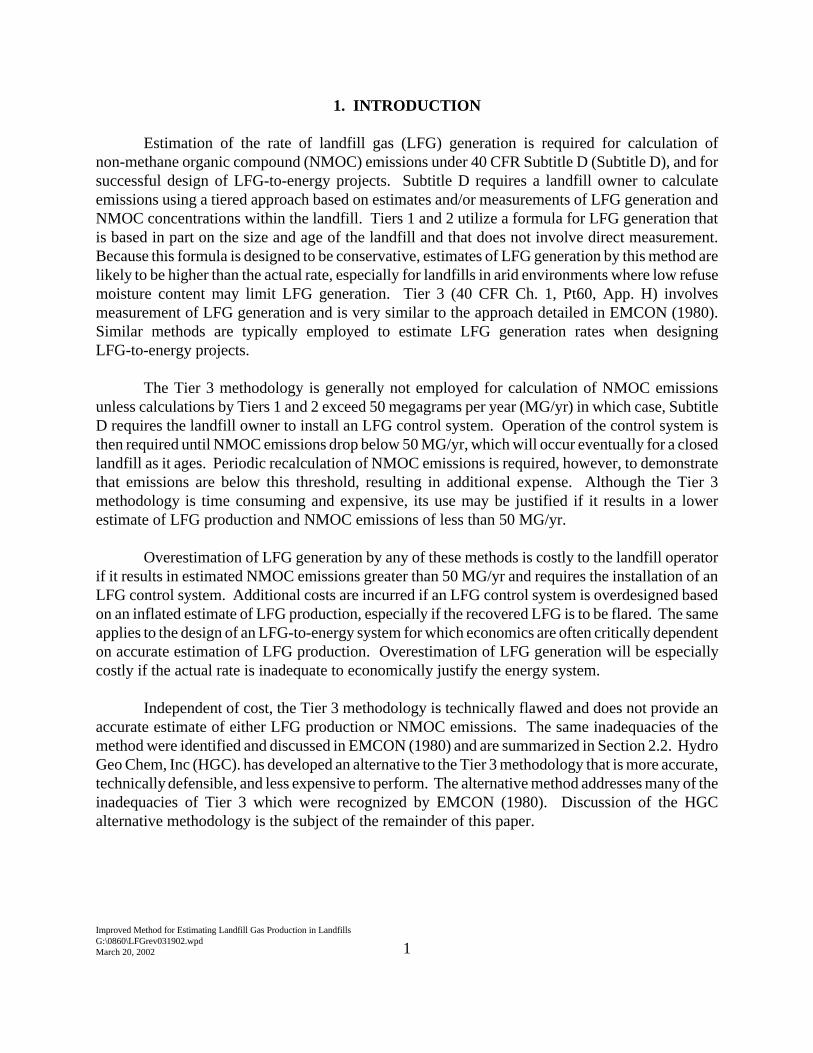
Estimation of the rate of landfill gas (LFG) generation is required for calculation ofnon-methane organic compound (NMOC) emissions under 40 CFR Subtitle D (Subtitle D), and forsuccessful design of LFG-to-energy projects. Subtitle D requires a landfill owner to calculateemissions using a tiered approach based on estimates and/or measurements of LFG generation andNMOC concentrations within the landfill. Tiers 1 and 2 utilize a formula for LFG generation thatis based in part on the size and age of the landfill and that does not involve direct measurement.Because this formula is designed to be conservative, estimates of LFG generation by this method arelikely to be higher than the actual rate, especially for landfills in arid environments where low refusemoisture content may limit LFG generation. Tier 3 (40 CFR Ch. 1, Pt60, App. H) involvesmeasurement of LFG generation and is very similar to the approach detailed in EMCON (1980).Similar methods are typically employed to estimate LFG generation rates when designingLFG-to-energy projects.

The Tier 3 methodology is generally not employed for calculation of NMOC emissionsunless calculations by Tiers 1 and 2 exceed 50 megagrams per year (MG/yr) in which case, SubtitleD requires the landfill owner to install an LFG control system. Operation of the control system isthen required until NMOC emissions drop below 50 MG/yr, which will occur eventually for a closedlandfill as it ages. Periodic recalculation of NMOC emissions is required, however, to demonstratethat emissions are below this threshold, resulting in additional expense. Although the Tier 3methodology is time consuming and expensive, its use may be justified if it results in a lowerestimate of LFG production and NMOC emissions of less than 50 MG/yr.

Overestimation of LFG generation by any of these methods is costly to the landfill operatorif it results in estimated NMOC emissions greater than 50 MG/yr and requires the installation of anLFG control system. Additional costs are incurred if an LFG control system is overdesigned basedon an inflated estimate of LFG production, especially if the recovered LFG is to be flared. The sameapplies to the design of an LFG-to-energy system for which economics are often critically dependenton accurate estimation of LFG production. Overestimation of LFG generation will be especiallycostly if the actual rate is inadequate to economically justify the energy system.

Independent of cost, the Tier 3 methodology is technically flawed and does not provide anaccurate estimate of either LFG production or NMOC emissions. The same inadequacies of themethod were identified and discussed in EMCON (1980) and are summarized in Section 2.2. HydroGeo Chem, Inc (HGC). has developed an alternative to the Tier 3 methodology that is more accurate,technically defensible, and less expensive to perform. The alternative method addresses many of theinadequacies of Tier 3 which were recognized by EMCON (1980). Discussion of the HGCalternative methodology is the subject of the remainder of this paper.


I P Pe= −0(1)

2. BACKGROUND

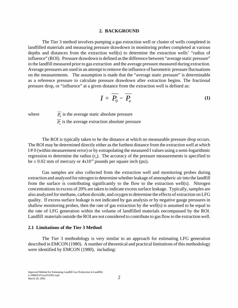
The Tier 3 method involves pumping a gas extraction well or cluster of wells completed inlandfilled materials and measuring pressure drawdown in monitoring probes completed at variousdepths and distances from the extraction well(s) to determine the extraction wells’ “radius ofinfluence” (ROI). Pressure drawdown is defined as the difference between “average static pressure”in the landfill measured prior to gas extraction and the average pressure measured during extraction.Average pressures are used in an attempt to remove the influence of barometric pressure fluctuationson the measurements. The assumption is made that the “average static pressure” is determinableas a reference pressure to calculate pressure drawdown after extraction begins. The fractionalpressure drop, or “influence” at a given distance from the extraction well is defined as:

where is the average static absolute pressureP0

is the average extraction absolute pressurePe

The ROI is typically taken to be the distance at which no measurable pressure drop occurs.The ROI may be determined directly either as the furthest distance from the extraction well at whichI # 0 (within measurement error) or by extrapolating the measured I values using a semi-logarithmicregression to determine the radius (re). The accuracy of the pressure measurements is specified tobe ± 0.02 mm of mercury or 4x10-4 pounds per square inch (psi).

Gas samples are also collected from the extraction well and monitoring probes duringextraction and analyzed for nitrogen to determine whether leakage of atmospheric air into the landfillfrom the surface is contributing significantly to the flow to the extraction well(s). Nitrogenconcentrations in excess of 20% are taken to indicate excess surface leakage. Typically, samples arealso analyzed for methane, carbon dioxide, and oxygen to determine the effects of extraction on LFGquality. If excess surface leakage is not indicated by gas analysis or by negative gauge pressures inshallow monitoring probes, then the rate of gas extraction by the well(s) is assumed to be equal tothe rate of LFG generation within the volume of landfilled materials encompassed by the ROI.Landfill materials outside the ROI are not considered to contribute to gas flow to the extraction well.

2.1 Limitations of the Tier 3 Method

The Tier 3 methodology is very similar to an approach for estimating LFG generationdescribed in EMCON (1980). A number of theoretical and practical limitations of this methodologywere identified by EMCON (1980), including:


1) “The validity of estimating the ROI from a semi-logarithmic extrapolation towithdrawal of gas from landfills remains to be verified.”

2) “A completely satisfactory method of estimating a landfill’s gas production rate fromextraction testing that draws only from a confined radius of influence has not beendemonstrated.”

3) “The influence of gas withdrawal [actually] extends to the limits of the landfillboundary (and beyond).”

4) “The distance taken as the ‘radius of influence’ depends on the precision of theinstruments used to measure landfill gas pressures and on the effects of diurnal(barometric) pressure fluctuations.”

With regard to the effect of barometric pressure fluctuations on calculation of pressuredrawdown, the Tier 3 technique specified under Subtitle D attempts to account for the effects ofchanging barometric pressure by specifying that barometric pressure be monitored and included inthe drawdown calculations. This is accomplished by adding landfill gauge pressure readings to thebarometric pressure readings during the “static” measurement period (prior to gas extraction) andduring gas extraction (yielding absolute pressure), and comparing the average pre-extraction andextraction period pressures to determine the radial distance at which the absolute pressure in thelandfill is not affected by pumping. However, if the average barometric pressure before extractiondiffers from the average pressure during extraction, the ROI will be either under- or over-estimated.This point will be discussed in more detail later.

EMCON (1980) further suggests that: “An accurate theoretical mass balance on the landfill gas remains to be developed and wouldprove invaluable in making such estimates [of landfill gas production]. The mass-balancecould account for refuse characteristics (e.g. permeability) and continuous gas production,the gas composition and extraction rate and the observed internal landfill pressure (orinfluence) distribution could be related to available equations for convective and diffusivegas flow, accounting for recovery, efficiency, and loss of gas to the atmosphere as a functionof distance from extraction well, landfill geometry, cover conditions, etc.”

These factors notwithstanding, the Tier 3 methodology rests entirely on the assumption thatthe gas extraction rate equals the LFG generation rate within the volume of the refuse between theextraction well and the ROI . This assumption is inconsistent with fundamental principles of gasflow to wells. To illustrate this point, assume that the LFG generation rate is uniform throughoutthe landfill and that the effective gas permeability of the refuse is much larger than the gaspermeability of the cover so that the vertical pressure gradient in the refuse is negligible. In this case,the average difference in pressure between refuse and the atmosphere due to flow through the coveris given simply by Darcy’s Law (Al-Hussainy and others, 1966):


qk P

bLFGc

c

=µ

∆(2)

∆ PQ

k bP re

e

r rD=

µπ2

( ) (4)

P K r B Bk b b

kDr r c

c= =

0

1 2

( / );/

(5)

∆ Pq b

kLFG c

c

=µ

(3)

orwhere qLFG is the gas generation rate per square foot of landfill

kc is the effective gas permeability of the cover µ is the dynamic viscosity of the LFGbc is the cover thickness?P is the pressure differential P Pa0 −

Pa is the atmospheric pressure

Given the assumption of a uniform LFG generation rate and an areally extensive landfill, the staticpressure in the refuse is and is uniform throughout the landfill. P P Pa0 0= + ∆

For small pressure differentials, the pressure drop created by the extraction well (assumingan ideal gas and steady-flow conditions and ignoring compressibility effects) is given by:

where kr is the effective horizontal air permeability of the refuse,Qe is the well extraction rate,PD(r) is an appropriate dimensionless pressure solution for flow to the well,?Pe is the difference between static and flowing pressure, andbr is the thickness of the refuse.

For the case of a highly permeable refuse in a lined landfill within relatively low permeabilitycover, the appropriate PD function is that given by Hantush (1964) for a leaky, confined formationwithout fluid storage in the confining bed:

where K0 is the modified Bessel function of zero order


∆Pq b

kQ

k bK r BLFG c

c

e

r re= =

µ µπ2 0( / ) (8)

∆ PQ

k bK r Be

e

r r

=µ

π2 0( / ) (6)

∆ PQ

k bK r Be

e

r re≅ =0

2 0

µπ

( / ) (7)

Thus, (4) becomes

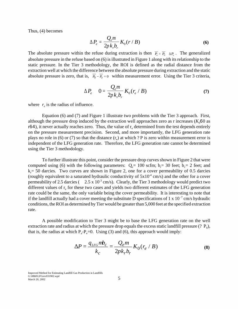
The absolute pressure within the refuse during extraction is then . The generalizedP P Pe e= +0 ∆

absolute pressure in the refuse based on (6) is illustrated in Figure 1 along with its relationship to thestatic pressure. In the Tier 3 methodology, the ROI is defined as the radial distance from theextraction well at which the difference between the absolute pressure during extraction and the staticabsolute pressure is zero, that is, within measurement error. Using the Tier 3 criteria,P Pe0 0− =

where re is the radius of influence.

Equation (6) and (7) and Figure 1 illustrate two problems with the Tier 3 approach. First,although the pressure drop induced by the extraction well approaches zero as r increases (K060 asr64), it never actually reaches zero. Thus, the value of re determined from the test depends entirelyon the pressure measurement precision. Second, and more importantly, the LFG generation rateplays no role in (6) or (7) so that the distance (re) at which ? P is zero within measurement error isindependent of the LFG generation rate. Therefore, the LFG generation rate cannot be determinedusing the Tier 3 methodology.

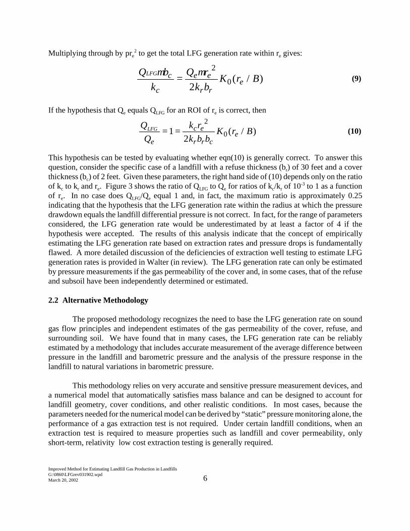
To further illustrate this point, consider the pressure drop curves shown in Figure 2 that werecomputed using (6) with the following parameters: Qe= 100 scfm; br= 30 feet; bc= 2 feet; andkr= 50 darcies. Two curves are shown in Figure 2, one for a cover permeability of 0.5 darcies(roughly equivalent to a saturated hydraulic conductivity of 5x10-4 cm/s) and the other for a coverpermeability of 2.5 darcies (ï 2.5 x 10-3 cm/s). Clearly, the Tier 3 methodology would predict twodifferent values of re for these two cases and yields two different estimates of the LFG generationrate could be the same, the only variable being the cover permeability. It is interesting to note thatif the landfill actually had a cover meeting the substitute D specifications of 1 x 10 -7 cm/s hydraulicconditions, the ROI as determined by Tier would be greater than 5,000 feet at the specified extractionrate.

A possible modification to Tier 3 might be to base the LFG generation rate on the wellextraction rate and radius at which the pressure drop equals the excess static landfill pressure (? P0),that is, the radius at which Pa-Pe=0. Using (3) and (6), this approach would imply:


Q bk

Q rk b

K r BLFG c

c

e e

r re

µ µ=

2

02( / ) (9)

QQ

k rk b b

K r BLFG

e

c e

r r ce= =1

2

2

0( / ) (10)

Multiplying through by pre2 to get the total LFG generation rate within re gives:

If the hypothesis that Qe equals QLFG for an ROI of re is correct, then

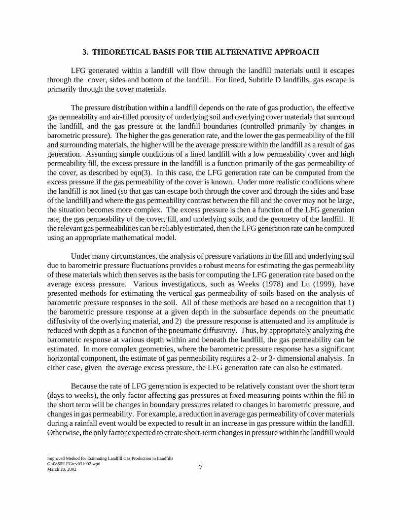
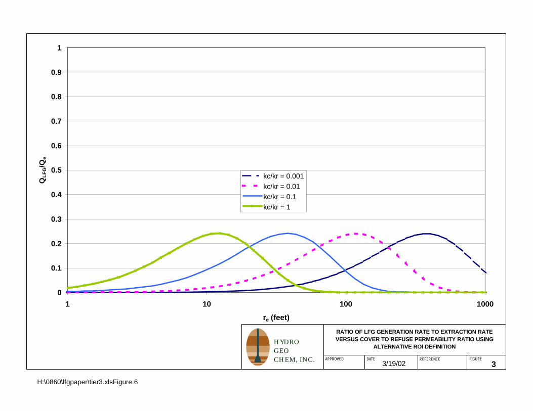
This hypothesis can be tested by evaluating whether eqn(10) is generally correct. To answer thisquestion, consider the specific case of a landfill with a refuse thickness (br) of 30 feet and a coverthickness (bc) of 2 feet. Given these parameters, the right hand side of (10) depends only on the ratioof kc to kr and re. Figure 3 shows the ratio of QLFG to Qe for ratios of kc/kr of 10-3 to 1 as a functionof re. In no case does QLFG/Qe equal 1 and, in fact, the maximum ratio is approximately 0.25indicating that the hypothesis that the LFG generation rate within the radius at which the pressuredrawdown equals the landfill differential pressure is not correct. In fact, for the range of parametersconsidered, the LFG generation rate would be underestimated by at least a factor of 4 if thehypothesis were accepted. The results of this analysis indicate that the concept of empiricallyestimating the LFG generation rate based on extraction rates and pressure drops is fundamentallyflawed. A more detailed discussion of the deficiencies of extraction well testing to estimate LFGgeneration rates is provided in Walter (in review). The LFG generation rate can only be estimatedby pressure measurements if the gas permeability of the cover and, in some cases, that of the refuseand subsoil have been independently determined or estimated.

2.2 Alternative Methodology

The proposed methodology recognizes the need to base the LFG generation rate on soundgas flow principles and independent estimates of the gas permeability of the cover, refuse, andsurrounding soil. We have found that in many cases, the LFG generation rate can be reliablyestimated by a methodology that includes accurate measurement of the average difference betweenpressure in the landfill and barometric pressure and the analysis of the pressure response in thelandfill to natural variations in barometric pressure.

This methodology relies on very accurate and sensitive pressure measurement devices, anda numerical model that automatically satisfies mass balance and can be designed to account forlandfill geometry, cover conditions, and other realistic conditions. In most cases, because theparameters needed for the numerical model can be derived by “static” pressure monitoring alone, theperformance of a gas extraction test is not required. Under certain landfill conditions, when anextraction test is required to measure properties such as landfill and cover permeability, onlyshort-term, relativity low cost extraction testing is generally required.


3. THEORETICAL BASIS FOR THE ALTERNATIVE APPROACH

LFG generated within a landfill will flow through the landfill materials until it escapesthrough the cover, sides and bottom of the landfill. For lined, Subtitle D landfills, gas escape isprimarily through the cover materials.

The pressure distribution within a landfill depends on the rate of gas production, the effectivegas permeability and air-filled porosity of underlying soil and overlying cover materials that surroundthe landfill, and the gas pressure at the landfill boundaries (controlled primarily by changes inbarometric pressure). The higher the gas generation rate, and the lower the gas permeability of the filland surrounding materials, the higher will be the average pressure within the landfill as a result of gasgeneration. Assuming simple conditions of a lined landfill with a low permeability cover and highpermeability fill, the excess pressure in the landfill is a function primarily of the gas permeability ofthe cover, as described by eqn(3). In this case, the LFG generation rate can be computed from theexcess pressure if the gas permeability of the cover is known. Under more realistic conditions wherethe landfill is not lined (so that gas can escape both through the cover and through the sides and baseof the landfill) and where the gas permeability contrast between the fill and the cover may not be large,the situation becomes more complex. The excess pressure is then a function of the LFG generationrate, the gas permeability of the cover, fill, and underlying soils, and the geometry of the landfill. Ifthe relevant gas permeabilities can be reliably estimated, then the LFG generation rate can be computedusing an appropriate mathematical model.

Under many circumstances, the analysis of pressure variations in the fill and underlying soildue to barometric pressure fluctuations provides a robust means for estimating the gas permeabilityof these materials which then serves as the basis for computing the LFG generation rate based on theaverage excess pressure. Various investigations, such as Weeks (1978) and Lu (1999), havepresented methods for estimating the vertical gas permeability of soils based on the analysis ofbarometric pressure responses in the soil. All of these methods are based on a recognition that 1)the barometric pressure response at a given depth in the subsurface depends on the pneumaticdiffusivity of the overlying material, and 2) the pressure response is attenuated and its amplitude isreduced with depth as a function of the pneumatic diffusivity. Thus, by appropriately analyzing thebarometric response at various depth within and beneath the landfill, the gas permeability can beestimated. In more complex geometries, where the barometric pressure response has a significanthorizontal component, the estimate of gas permeability requires a 2- or 3- dimensional analysis. Ineither case, given the average excess pressure, the LFG generation rate can also be estimated.

Because the rate of LFG generation is expected to be relatively constant over the short term(days to weeks), the only factor affecting gas pressures at fixed measuring points within the fill inthe short term will be changes in boundary pressures related to changes in barometric pressure, andchanges in gas permeability. For example, a reduction in average gas permeability of cover materialsduring a rainfall event would be expected to result in an increase in gas pressure within the landfill.Otherwise, the only factor expected to create short-term changes in pressure within the landfill would


∂∂ φµ

∂∂

Pt

k P Pz

a a2 2 2

2= (11)

P A t Pa2 2= + + +sin( )ω ε θ (12)

be changes in boundary pressure resulting from barometric pressure fluctuations. Under unusualconditions, however, rainfall infiltration into the refuse could increase LFG generation.

Based on fluid flow principles and observation, changes in barometric pressure propagatingthrough porous materials undergo a phase shift (or lag) and an attenuation in amplitude(Weeks,1978). The lag and amplitude attenuation increase with depth. The lag and attenuationdepend on the vertical permeability and porosity of the subsurface materials, withlower-permeability, higher-porosity materials resulting in greater attenuation of the response.

Under simple conditions where the airflow can be assumed to be only vertical, and theeffective air permeability of the cover, refuse, and underlying soil are uniform, the pressuredistribution is governed by the following differential equation:

where is the average pressure.Pa

If the variation in barometric pressure is assumed to be a simple harmonic function and thewater table acts as an impermeable boundary to air flow, then the temporal variations in pressure inthe subsurface is given by (Lu, 1999):

where A is the amplitude of the pressure variation at depth z? is the phase lag at depth zg is the initial phase lag.

Both A and ? are related to functions of the pneumatic diffusivity, byK Pa a / ,θµtranscendental functions that are not reported here. Nevertheless, if the porosity can beindependently estimated, (12) provides a basis for estimating the vertical pneumatic diffusivity andvertical air permeability based on an analysis of barometric pressure signals at depth. Equation (12)also indicates that the excess landfill pressure can be determined by separating the barometricpressure response from the excess landfill pressure or by long-term pressure averaging of theabsolute pressure and the LFG generation rate determined from the excess landfill pressure using (3).

Unfortunately, this simple approach is not feasible under most landfill conditions because:1. the vertical air permeability is not uniform,2. the barometric pressure signal is not a simple harmonic function, and3. the air flow is not strictly vertical.


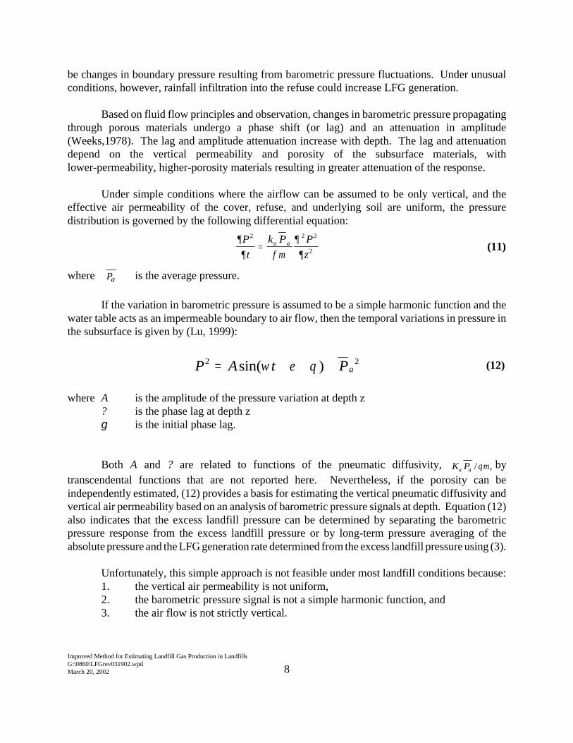
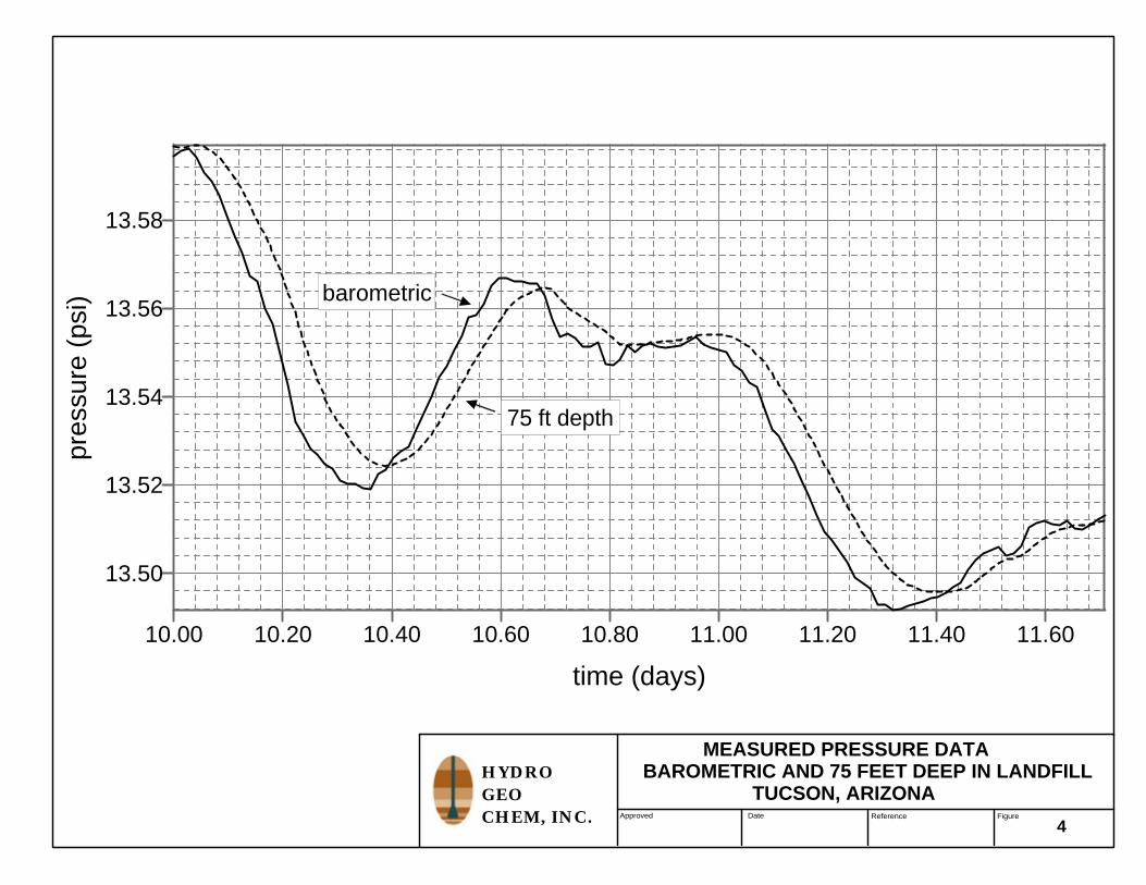
The first limitation is obvious because the subsurface materials at a landfill typically consistof relatively low permeability cover, highly-permeable refuse, and lower-permeability subsoil. Thesecond limitation is illustrated by Figure 4 which shows the non-harmonic barometric pressure andsubsurface pressure response of a landfill in Tucson, Arizona. The final limitation related to verticalair flow will be discussed later.

These limitations can be overcome, however, by analyzing the pressure response using anumerical model. The measured barometric pressure is imposed as a boundary condition, and thepermeabilities and porosities of the fill and surrounding materials adjusted until the simulatedpressure at the fixed measurement point has the same lag and amplitude attenuation as the measuredpressure. Because the porosity of the landfill and surrounding materials will vary less than thepermeability, reasonable values for porosity can usually be assumed and changes in the signalattributed only to the permeability distribution. The calculated permeability distribution and LFGgeneration rates will, of course, depend on the accuracy of the porosity estimate. If necessary, theuncertainty associated with the porosity estimate can be reduced by performing extraction well teststo independently estimate the refuse and cover permeabilities.

The procedure is simplified for Subtitle D landfills which have low permeability liners,because movement of gas through the underlying soil does not need to be considered. Once thepermeabilities of the fill and surrounding materials have been estimated, the measured increase inpressure resulting from LFG production can be used to estimate the rate of LFG production usingthe gas flow model. This is possible because the increase in pressure resulting from constant gasgeneration (which can be considered a steady-state effect) adds a constant to the pressure responsemeasured in the landfill, but does not result in a lag or attenuation in amplitude of the signal. Thisbehavior is illustrated empirically and numerically in Figure 5, which displays the results of asimulation performed at a landfill site in Tucson. In this case, LFG generation results in a constantpressure excess of 4 x 10-3 psi within the landfill over a period of 2 days. The excess pressure isdependent on the LFG generation rate through Darcy’s Law as described previously. Although thelandfill at this site was unlined and had a relatively high permeability cover, sufficient lag andattenuation in the signal were present to estimate both permeability of landfill and cover and theLFG generation rate. As will be discussed in Section 4, this represents the most difficult case inwhich to apply the method.

1Note that 1 darcy is approximately equal to a water saturated hydraulic conductivity of 10-3 cm/s.


4. DEMONSTRATION OF THE METHOD

The LFG production measurement technique presented here is demonstrated for sixhypothetical cases using TRACRN, a three-dimensional finite difference computer code developedat Los Alamos National Laboratories, that is capable of simulating gas and liquid flow, and solutetransport, under conditions of variable water saturation (Travis and Birdsell, 1988). The sixhypothetical cases that were simulated are described in Table 1. Three of the cases represent unlinedlandfills and three represent lined landfills. In all cases, the gas permeability of the fill is assumedto be high (50 darcies horizontal, 10 darcies vertical), the permeability of the surrounding soil to berelatively high (20 darcies horizontal, 2 darcies vertical), and the permeability of the cover variable,ranging from 10-2 darcies to 10 darcies1. The porosity is assumed to be constant for the variouscases. In our experience, fill materials generally have high permeability but cover permeabilitiesvary substantially between landfills. The lower cover permeabilities are more representative ofSubtitle D landfills than older landfills that are also typically unlined. Furthermore, variations inporosity are much less than variations in permeability, which can vary over several orders ofmagnitude, and were therefore not considered in the simulations.

A cross-section showing the simulated landfill geometry is provided in Figure 6. One halfof the 60-foot thick landfill is located above grade, and one half is below grade. The sides of theabove-grade portion of the simulated landfill have a slope of approximately 7E. The footprint of thelandfill is 2,000 feet in diameter and is symmetrical.

4.1 Description of the Numerical Model

Two numerical models were constructed to represent the various cases, a two-dimensional,radially-symmetric model in which the footprint of the landfill is a circle with diameter of 2,000 feet,and a three-dimensional model in which the footprint of the model is a square 2,000 feet on a side.The two-dimensional model was radially symmetric, and consisted of an array of 40 non-equallyspaced cells in the radial direction, and 18 non-equally spaced layers. Layers in which landfillmaterial was represented were uniformly 5 feet thick. The model boundary was located 2,000 feetfrom the sides of the landfill to minimize boundary effects. The three-dimensional model consistedof a rectangular array of 48 non-equally spaced cells in the x direction, 48 non-equally spaced cellsin the y direction, and 18 non-equally spaced layers. The x and y spacing within the arearepresenting the landfill was uniformly 50 feet, and the layer thickness uniformly 5 feet. Modelboundaries were located 1,500 feet from the sides of the landfill to minimize boundary effects.

One hundred and seventy feet of vadose zone soils were represented beneath the landfill inboth the two-dimensional and three-dimensional model representations. The lower boundary wasspecified no-flow to represent the water table. Side boundaries (located far from the landfillmargins) were also no-flow, and the upper boundary specified at atmospheric pressure. In both


models, the materials outside the landfill boundary that were below grade represented native soils,and the materials above grade represented “air,” specified as a very high permeability, high porositymaterial. Properties of the materials represented in the model are provided in Table 2.

In both the two-dimensional and three-dimensional representations, landfill gas generationwas simulated by specifying a constant gas source in each cell representing landfill material. Thesource strength for all landfill cells in the three-dimensional model, which were of equal volume,was the same. The source strength specified for landfill cells in the two-dimensional model wasvaried according to cell volume to maintain a constant ratio of source strength to cell volume. Thetotal gas generation rate for the two-dimensional model was approximately 1,750 scfm, and for thethree-dimensional model, 2,300 scfm (because of larger volume).

A barometric pressure signal (shown in Figure 7) was applied at the upper boundary of eachmodel. The signal consisted of actual pressures measured at hourly intervals at a site in Tucson.When gas generation was simulated, the pressure at the upper boundary was fixed at the averagesignal pressure until steady-state conditions developed, then the varying barometric pressure signalwas applied. The varying barometric pressure signal was transmitted through the sides of the landfillabove grade, and the soils represented in the model, via the material representing “air”.Transmission of the barometric pressure signal through materials representing “air” is nearlyinstantaneous due to the high permeability of the material.

The two-dimensional radial model was designed with a cell spacing that was narrow at thecenter of the model, and widened radially outward toward the landfill boundaries. The materialproperties of the center nodes were specified such that the nodes could function as a gas extractionwell or pressure monitoring probe in a manner representative of the way such a probe or well wouldfunction in the field.

Because of the symmetrical geometry of both the two-dimensional and three-dimensionalrepresentations, the two-dimensional model worked equally well for illustrating the techniquedescribed in the previous section, and with much less computational effort than thethree-dimensional model. The two-dimensional model was also well-suited to simulating a Tier 3type gas extraction test when the extraction well was located at the center of the landfill. Thethree-dimensional model, because it contained “corners” that would occur in actual landfills, wasmainly useful for investigation of edge effects or for simulating more complex landfill geometriesthat are not considered here.

4.2 Simulation of the Technique

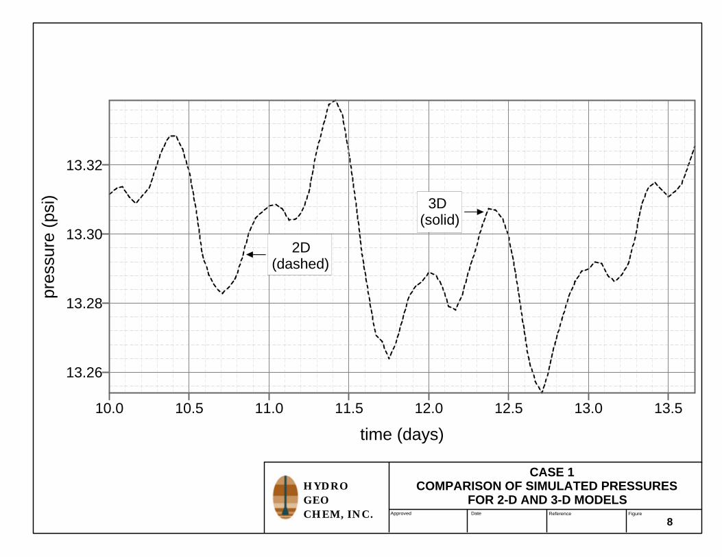
The six cases listed in Table 1 were simulated using the two-dimensional model, and, forcomparison, cases 1 and 3 were also simulated using the three-dimensional model. For thecomparison case, the barometric signal was applied and absolute pressures measured at a depth of30 feet at the center of the landfill in both the two-dimensional and three-dimensional models.


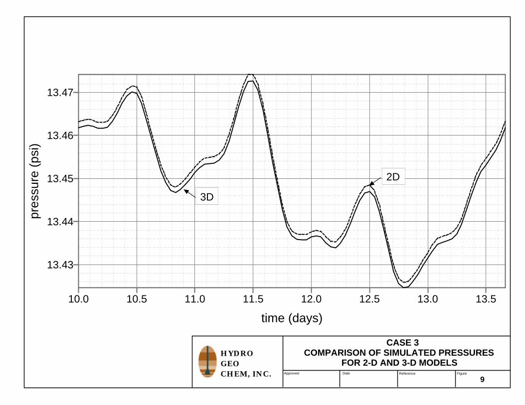
Figures 8 and 9 show the results of these simulations. As indicated in Figure 9, slightly higherpressures result from the two-dimensional model, although the source strength/volume ratio is thesame for both. This difference is due to the higher surface area/volume ratio for thethree-dimensional, rectangular model relative to the two-dimensional, cylindrical model, andillustrates the importance of taking landfill geometry into account.

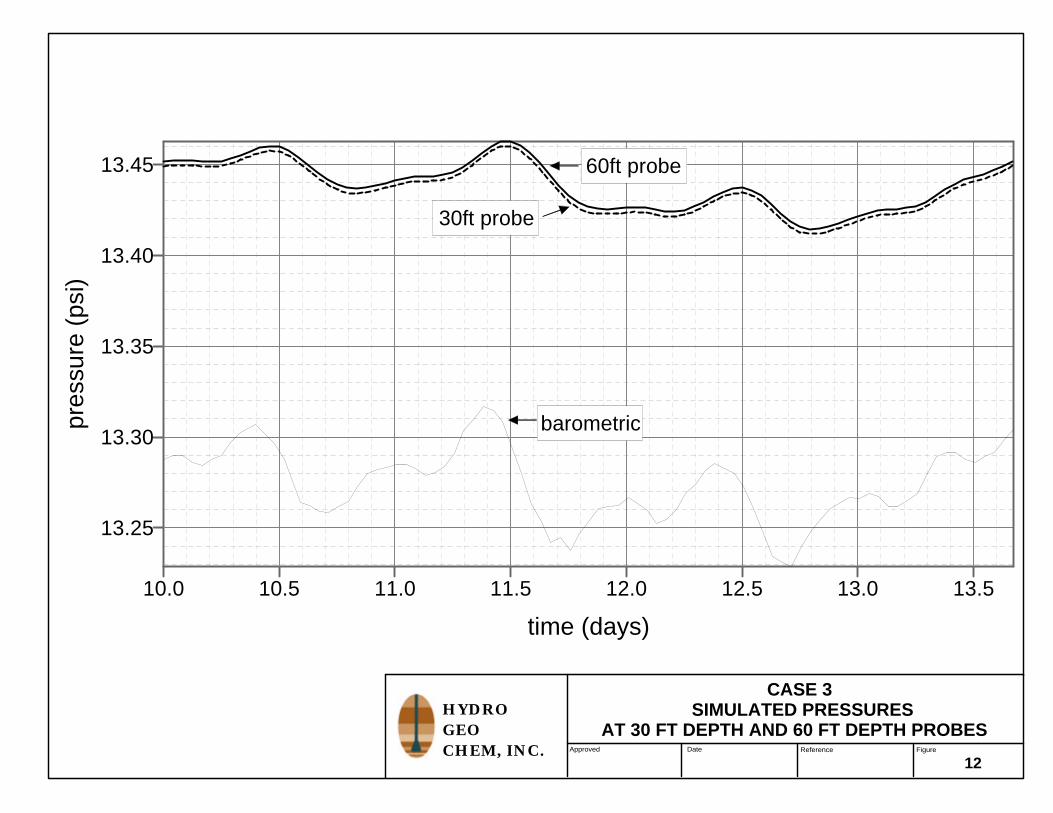
The six cases were simulated using the two-dimensional model, with and without gasgeneration, and with application of the barometric signal. Simulated pressures were monitored inpressure monitoring probes completed a depths of 30 feet and 60 feet in the center of the landfill.Results of the simulations are depicted in Figures 10 through 15.

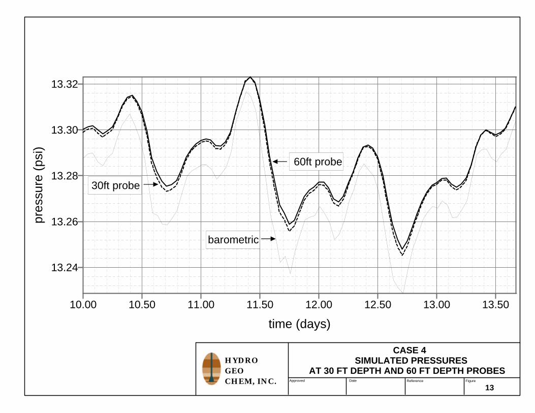
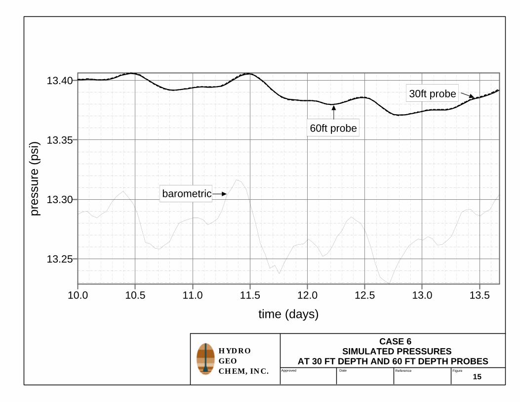
As indicated, the pressure lag and amplitude attenuation increase with decreasing cappermeability, and are accentuated by the presence of a liner. In the cases with the high permeabilitycover (cases 1 and 4), almost no measurable lag or attenuation occurs in the signal. Furthermore,there is almost no lag or attenuation between the simulated signals at 30 foot and 60 foot depths inthe landfill because of the high permeability of the landfill materials.

The increase in pressure within the landfill relative to atmospheric pressure (shown by theupward translation of pressure curves in simulations with gas generation) is due to the gas sourcewithin the landfill. As shown in Figures 10 through 15, the effect of the gas generation is to translatethe pressure curves upward without producing any change in shape (lag or amplitude attenuation)of the curves. This is an important observation that illustrates the separability of the steady-state andtransient effects.

The results of the simulations show that under conditions where landfill permeability is high(>10 darcies) and cover permeability is relatively low (10-2 to 1 darcy), and porosity variations canbe ignored, the lag and attenuation in amplitude of the barometric signal transmitted to the landfillare sufficient to determine the permeability of the cover material. In the cases of the lined landfills,where nearly all gas escapes through the cover, only the cover permeability needs to be determinedto estimate the gas generation rate based on the measured pressure increase in the landfill relativeto atmospheric pressure. The lag and attenuation of the signal that results from transmission throughthe high permeability landfill materials is insignificant in these cases and can be ignored.

In the case where the cover permeability is nearly the same as the landfill permeability, thepermeability of both must be determined to estimate the gas generation rate. As shown in Figures 10and 13, there may not be sufficient information in the signal to estimate permeability, except toestablish a lower limit. In such cases, an independent method for estimating permeability may berequired for accurate estimation of gas generation. This is accomplished by performing a gasextraction test on a gas extraction well completed in the landfill. By measuring pressure drawdownat monitoring points completed at various depths in the fill during gas extraction, and analyzing thepressure response with an appropriate well pneumatics model, the horizontal and verticalpermeability of the fill (and cap permeability) can be estimated. Generally, these tests require only


one to two hours of gas extraction and pressure monitoring to collect sufficient information forpermeability estimation. Although in many cases where the landfill is unlined and has a relativelyhigh permeability cover, a gas extraction test will be required, this is not always the case as was seenat the landfill site in Tucson discussed in Section 3 (Figures 4 and 5).

In the case of an unlined landfill, gas movement through the sides of the landfill below gradeand through the base of the landfill must also be considered in estimating gas generation rates. Thiscan be accomplished by a combination of barometric tests on probes completed in native soils at thesite, and extraction tests on wells completed in the soils. The level of testing necessary will dependon specific site conditions and the results of initial barometric tests on the landfill itself. Clearly,most Subtitle D landfills that have liners and low permeability covers will require only barometrictests; as will unlined landfills completed in low permeability native soils.

4.3 Demonstration of Problems Associated with Tier 3

As discussed previously, the Tier 3 methodology is not based on sound principles of fluidflow and is fundamentally flawed. To further quantify the errors in the Tier 3 methodology, Tier 3measurements of LFG production for selected cases listed in Table 2 were performed using thetwo-dimensional model. The simulations were performed to demonstrate the dependence of ROIestimation on the sensitivity of the pressure measuring equipment, on changes in barometricpressure, and on test duration, and to demonstrate that as stated by EMCON (1980) the effects of gasextraction actually extend to the landfill boundaries. As will be shown in section 4.3.1, this lasteffect essentially invalidates the usefulness of the concept of ROI for measurement of gas generationovershadowing other shortcomings in the technique. Furthermore, because the ROI will expand withincreasing pressure measurement sensitivity, the estimate of gas generation will be less and lessaccurate as the sensitivity of the pressure measurements increases.

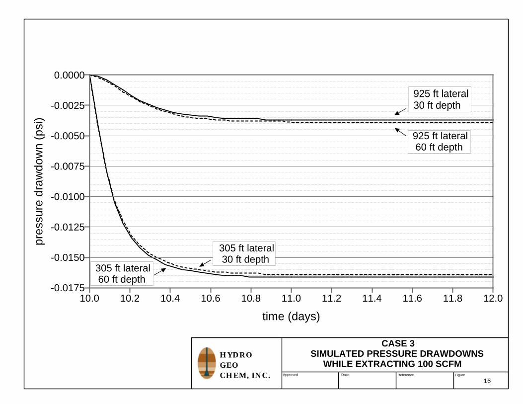
4.3.1 Dependence of ROI Estimation on Sensitivity of Pressure Measurement

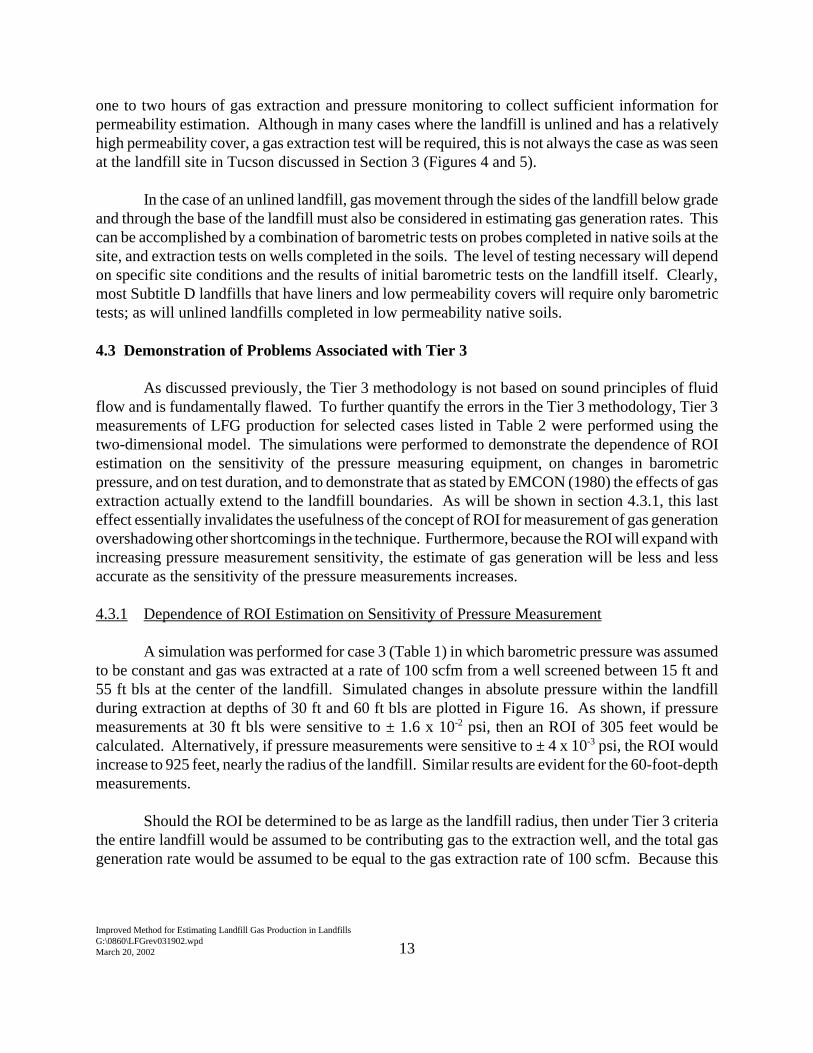
A simulation was performed for case 3 (Table 1) in which barometric pressure was assumedto be constant and gas was extracted at a rate of 100 scfm from a well screened between 15 ft and55 ft bls at the center of the landfill. Simulated changes in absolute pressure within the landfillduring extraction at depths of 30 ft and 60 ft bls are plotted in Figure 16. As shown, if pressuremeasurements at 30 ft bls were sensitive to ± 1.6 x 10-2 psi, then an ROI of 305 feet would becalculated. Alternatively, if pressure measurements were sensitive to ± 4 x 10-3 psi, the ROI wouldincrease to 925 feet, nearly the radius of the landfill. Similar results are evident for the 60-foot-depthmeasurements.

Should the ROI be determined to be as large as the landfill radius, then under Tier 3 criteriathe entire landfill would be assumed to be contributing gas to the extraction well, and the total gasgeneration rate would be assumed to be equal to the gas extraction rate of 100 scfm. Because this


PP P

nia

bar g

n

=+∑ ( )

1 (13)

PP P

nfa

bar g

n

=+∑ ( )

1 (14)

is only 6% of the actual total gas generation rate of 1,750 scfm, the rate would be underestimated bya factor of nearly 18.

4.3.2 Dependence of Tier 3 ROI Estimation on Changes in Barometric Pressure

The dependence of Tier 3 ROI estimation on changes in barometric pressure results from theassumption that “average static pressure” in the landfill can be determined prior to gas extraction andthat this is a relevant baseline against which to calculate pressure drawdown during gas extraction.The average static pressure is determined by measuring barometric pressure (Pbar) and the gaugepressure (Pg) in each monitoring probe every eight hours for several days prior to extraction, addingthe gauge readings to the barometric readings to get absolute pressures, and averaging the readingsat each probe to yield the average absolute static pressure Pia for each probe. An identical processis employed after extraction begins to yield the average absolute pressure Pfa during extraction. Theformula for calculating average static pressure at a measuring location is:

Where n = the number of readings,

and the formula for calculating average pressure at a measuring location during extraction is:

The average pressure calculation during extraction uses only those readings that werecollected at an extraction rate that does not induce excess surface leakage. The ROI is thendetermined as the maximum distance at which the average pressure during extraction (Pfa) is lessthan or equal to the average pressure prior to extraction (Pia). Clearly, however, the readings duringextraction depend on the magnitude of average barometric pressure which may vary during the timeof measurement.

Assuming landfill pressures respond to changes in barometric pressure, when the averagebarometric pressure is lower by a measurable amount during extraction, all average pressurescalculated for all measurement points will be lower than the calculated average static pressures andthe apparent ROI will extend to the landfill boundaries. Under these conditions, pressures wouldbe lower even if no gas were extracted. In the case where average barometric pressure is higherduring extraction, the calculated ROI would be smaller than if calculated at a time when average


barometric pressure was the same before and during extraction. The effect of barometric pressurechanges can only be taken into account in the calculations if the response of landfill pressure tochanges in barometric pressure is incorporated, for example, using a numerical model.

4.3.3 Dependence of Surface Leakage Detection on Length of Testing

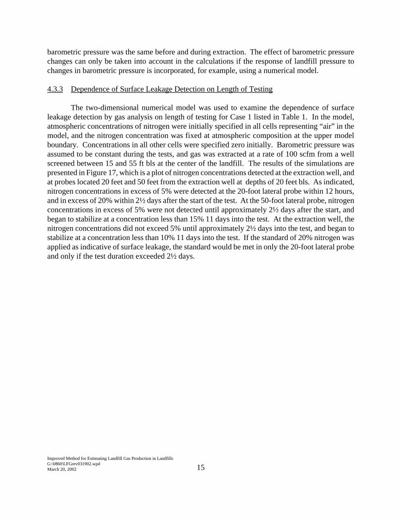
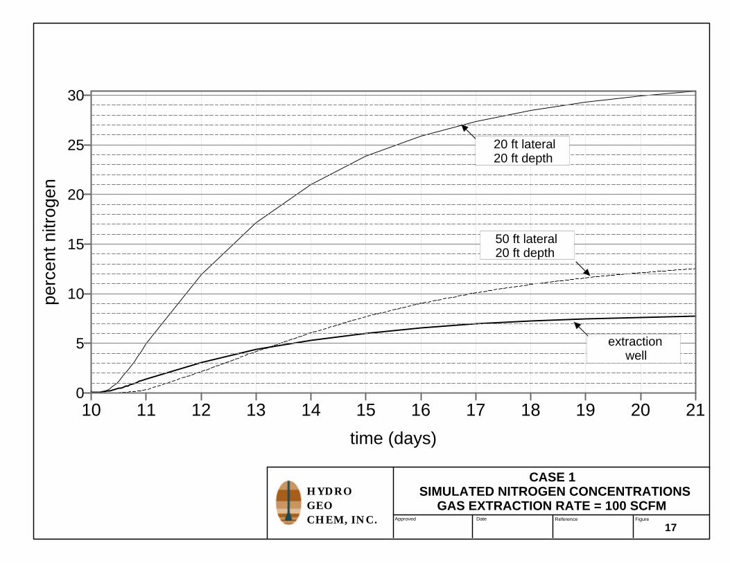
The two-dimensional numerical model was used to examine the dependence of surfaceleakage detection by gas analysis on length of testing for Case 1 listed in Table 1. In the model,atmospheric concentrations of nitrogen were initially specified in all cells representing “air” in themodel, and the nitrogen concentration was fixed at atmospheric composition at the upper modelboundary. Concentrations in all other cells were specified zero initially. Barometric pressure wasassumed to be constant during the tests, and gas was extracted at a rate of 100 scfm from a wellscreened between 15 and 55 ft bls at the center of the landfill. The results of the simulations arepresented in Figure 17, which is a plot of nitrogen concentrations detected at the extraction well, andat probes located 20 feet and 50 feet from the extraction well at depths of 20 feet bls. As indicated,nitrogen concentrations in excess of 5% were detected at the 20-foot lateral probe within 12 hours,and in excess of 20% within 2½ days after the start of the test. At the 50-foot lateral probe, nitrogenconcentrations in excess of 5% were not detected until approximately 2½ days after the start, andbegan to stabilize at a concentration less than 15% 11 days into the test. At the extraction well, thenitrogen concentrations did not exceed 5% until approximately 2½ days into the test, and began tostabilize at a concentration less than 10% 11 days into the test. If the standard of 20% nitrogen wasapplied as indicative of surface leakage, the standard would be met in only the 20-foot lateral probeand only if the test duration exceeded 2½ days.


5. CONCLUSIONS

The limitations of the Tier 3 methodology for estimating gas generation rates in landfills havebeen demonstrated in this paper, and HGC’s alternative methodology that avoids these limitations hasbeen presented. Most of the Tier 3 limitations discussed here were presented originally inEMCON (1980).

Specifically, the limitations of the Tier 3 methodology include:1) the theoretical basis is unsound,2) methodology is expensive and time consuming,3) estimates are inaccurate, and4) estimates decrease in accuracy as the sensitivity of the pressure measurement data

increases.

The alternative methodology is superior to Tier 3 for the following reasons. HGC’smethodology:

1) is theoretically sound,2) it is more accurate (and accuracy increases with pressure measurement sensitivity),

and3) the determined methodology can be performed at much lower cost in most situations.


6. REFERENCES

Al-Hussainy, R., H.J. Ramey, Jr., and P.B> Crawford. 1966. The Flow of Real Gases ThroughPorous Media. Journal of Petroleum Technology. Vol. 237:624-636.

Carslaw, H.S. and J.C. Jaeger. 1959. Conduction of Heat in Solids. Oxford University Press.Oxford, England.

Hantush, M.S. 1964. Hydraulics of Wells in Advances in Hydroscience, Volume I. V.T. Chow Ed.Academic Press, New York.

Lu, N. 1999. Time-series analysis for determining vertical air permeability in unsaturated zone.J. Geotechnical and Environmental Engineering. January. Pp. 69-67.

Rojstaczer, S. and J. Turk. 1995. Field-based determinations of air diffusivity using soil air andatmospheric pressure time series. Water Resources Research. Volume 31:3337-3343.

Travis, B.J. and H.H. Birdsell. 1988. TRACRN 1.0: A model of flow and transport in porousmedia for the Yucca Mountain Project. Los Alamos National Laboratories.TWS-ESS-5/10-88-08.

Walter, G.R. In review. Fatal flaws in measuring landfill gas generation rates by empirical welltesting. Submitted to Journal of the Air Waste Management Association.

Weeks, E.P. 1978. Field determination of vertical permeability to air in the unsaturated zone. U.S.Geological Survey Professional Paper 1051.

TABLES

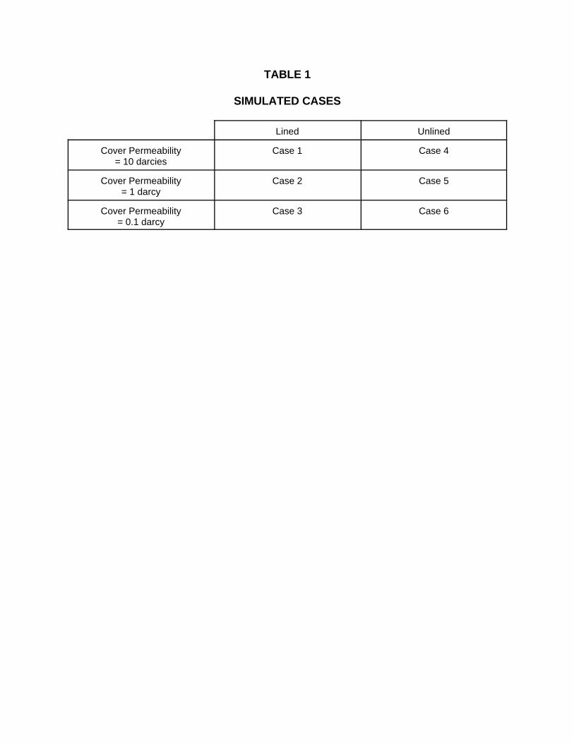
TABLE 1

SIMULATED CASES

Lined Unlined

Cover Permeability= 10 darcies

Case 1 Case 4

Cover Permeability= 1 darcy

Case 2 Case 5

Cover Permeability= 0.1 darcy

Case 3 Case 6

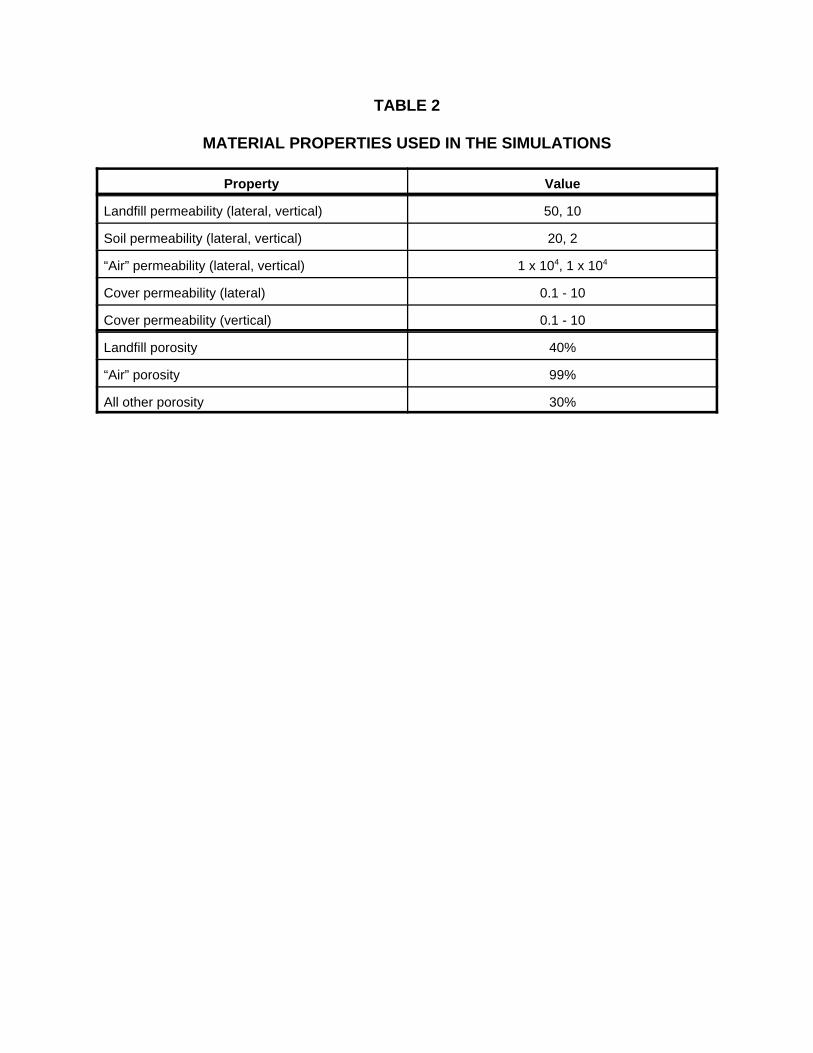
TABLE 2

MATERIAL PROPERTIES USED IN THE SIMULATIONS

Property Value

Landfill permeability (lateral, vertical) 50, 10

Soil permeability (lateral, vertical) 20, 2

“Air” permeability (lateral, vertical) 1 x 104, 1 x 104

Cover permeability (lateral) 0.1 - 10

Cover permeability (vertical) 0.1 - 10

Landfill porosity 40%

“Air” porosity 99%

All other porosity 30%

FIGURES

Distance From Well

Ab

solu

te P

ress

ure

HYDROGEOCHEM, INC. FIGUREDATEAPPROVED REFERENCE

Pressure in Refuse (Static Pressure)

Atmospheric Pressure (Pa)

re (P0 – Pe) ˜ 0

GENERALIZED PLOT OF PRESSURE VERSUS DISTANCE FROM A SINGLE

EXTRACTION WELL

1H:\0860\lfg paper\FIG 1 REV.PPT03/19/02

0

Pressure versus Distance from Well (Pe)

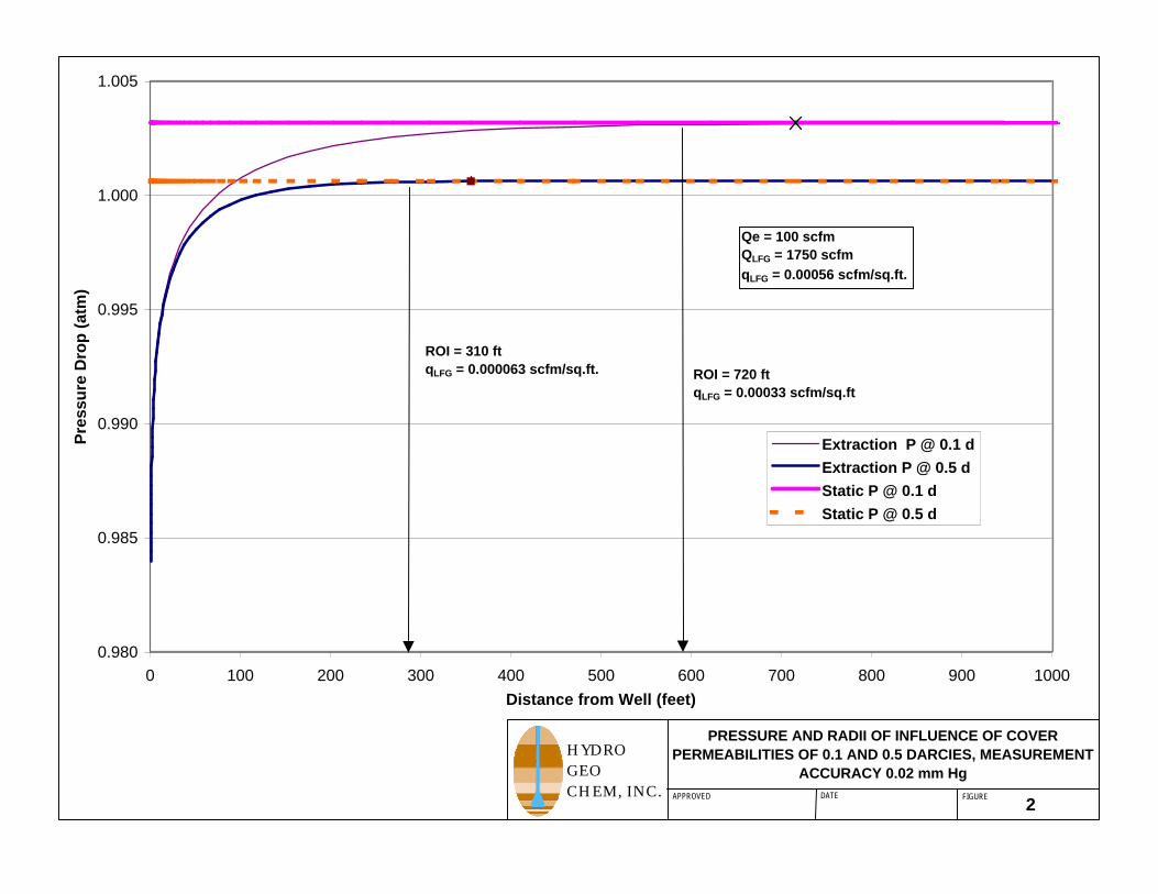
0.980

0.985

0.990

0.995

1.000

1.005

0 100 200 300 400 500 600 700 800 900 1000Distance from Well (feet)

Pre

ssu

re D

rop

(at

m)

Extraction P @ 0.1 dExtraction P @ 0.5 dStatic P @ 0.1 dStatic P @ 0.5 d

ROI = 310 ftqLFG = 0.000063 scfm/sq.ft. ROI = 720 ft

qLFG = 0.00033 scfm/sq.ft

Qe = 100 scfmQLFG = 1750 scfmqLFG = 0.00056 scfm/sq.ft.

PRESSURE AND RADII OF INFLUENCE OF COVER PERMEABILITIES OF 0.1 AND 0.5 DARCIES, MEASUREMENT

ACCURACY 0.02 mm Hg

HYDROGEOCHEM, INC. FIGUREDATEAPPROVED

2

H:\0860\lfgpaper\tier3.xlsFigure 6

0

0.1

0.2

0.3

0.4

0.5

0.6

0.7

0.8

0.9

1

1 10 100 1000

re (feet)

QL

FG/Q

e

kc/kr = 0.001kc/kr = 0.01kc/kr = 0.1kc/kr = 1

RATIO OF LFG GENERATION RATE TO EXTRACTION RATE VERSUS COVER TO REFUSE PERMEABILITY RATIO USING

ALTERNATIVE ROI DEFINITIONHYDROGEOCHEM, INC. FIGUREDATEAPPROVED REFERENCE

33/19/02

Approved Date Reference Figure

HYDROGEOCHEM, INC.

MEASURED PRESSURE DATABAROMETRIC AND 75 FEET DEEP IN LANDFILL TUCSON, ARIZONA

10.00 10.20 10.40 10.60 10.80 11.00 11.20 11.40 11.60

time (days)

13.50

13.52

13.54

13.56

13.58

pres

sure

(ps

i) barometric

75 ft depth

4


HYDROGEOCHEM, INC.

10.00 10.20 10.40 10.60 10.80 11.00 11.20 11.40 11.60

time (days)

13.50

13.52

13.54

13.56

13.58

pres

sure

(ps

i) simulated(with gas)

measured(open circles)

simulated(no gas)

SIMULATED RESULTS AT 75 FOOT DEPTH IN LANDFILL WITH AND WITHOUT

GAS GENERATION TUCSON, ARIZONA

5


HYDROGEOCHEM, INC.

-2000 -1500 -1000 -500 0 500 1000 1500 2000

lateral distance (feet)

-200

-160

-120

-80

-40

0

elev

atio

n (fe

et)

landfill'air' 'air'

unsaturated soil

water table

land surface land surface

SCHEMATIC CROSS-SECTION OF LANDFILL

6


HYDROGEOCHEM, INC.

10.0 10.5 11.0 11.5 12.0 12.5 13.0 13.5

time (days)

13.24

13.26

13.28

13.30

pres

sure

(ps

i)

BAROMETRIC PRESSURE SIGNAL USED IN SIMULATIONS

7


HYDROGEOCHEM, INC.

10.0 10.5 11.0 11.5 12.0 12.5 13.0 13.5

time (days)

13.26

13.28

13.30

13.32

pres

sure

(ps

i) 3D(solid)

2D(dashed)

CASE 1COMPARISON OF SIMULATED PRESSURES FOR 2-D AND 3-D MODELS

8


HYDROGEOCHEM, INC.

CASE 3COMPARISON OF SIMULATED PRESSURES FOR 2-D AND 3-D MODELS

10.0 10.5 11.0 11.5 12.0 12.5 13.0 13.5

time (days)

13.43

13.44

13.45

13.46

13.47

pres

sure

(ps

i)

2D

3D

9


HYDROGEOCHEM, INC.

10.0 10.5 11.0 11.5 12.0 12.5 13.0 13.5

time (days)

13.24

13.26

13.28

13.30

13.32

pres

sure

(ps

i)

barometric

30ft probe

60ft probe

CASE 1 SIMULATED PRESSURESAT 30 FT DEPTH AND 60 FT DEPTH PROBES

10


HYDROGEOCHEM, INC.

10.0 10.5 11.0 11.5 12.0 12.5 13.0 13.5

time (days)

13.24

13.26

13.28

13.30

13.32

13.34

pres

sure

(ps

i)

barometric

60ft probe

30ft probe


11


HYDROGEOCHEM, INC.

10.0 10.5 11.0 11.5 12.0 12.5 13.0 13.5

time (days)

13.25

13.30

13.35

13.40

13.45

pres

sure

(ps

i)

60ft probe

30ft probe

barometric


12


HYDROGEOCHEM, INC.

10.00 10.50 11.00 11.50 12.00 12.50 13.00 13.50

time (days)

13.24

13.26

13.28

13.30

13.32

pres

sure

(ps

i)

barometric

30ft probe

60ft probe


13


HYDROGEOCHEM, INC.

10.0 10.5 11.0 11.5 12.0 12.5 13.0 13.5

time (days)

13.24

13.26

13.28

13.30

13.32

pres

sure

(ps

i)

barometric

60ft probe

30ft probe


14


HYDROGEOCHEM, INC.

10.0 10.5 11.0 11.5 12.0 12.5 13.0 13.5

time (days)

13.25

13.30

13.35

13.40

pres

sure

(ps

i)

barometric

60ft probe

30ft probe


15


HYDROGEOCHEM, INC.

10.0 10.2 10.4 10.6 10.8 11.0 11.2 11.4 11.6 11.8 12.0

time (days)

-0.0175

-0.0150

-0.0125

-0.0100

-0.0075

-0.0050

-0.0025

0.0000

pres

sure

dra

wdo

wn

(psi

)

925 ft lateral30 ft depth

925 ft lateral 60 ft depth



CASE 3SIMULATED PRESSURE DRAWDOWNS WHILE EXTRACTING 100 SCFM

16


HYDROGEOCHEM, INC.

10 11 12 13 14 15 16 17 18 19 20 21

time (days)

0

5

10

15

20

25

30

perc

ent n

itrog

en

extraction well



CASE 1SIMULATED NITROGEN CONCENTRATIONS GAS EXTRACTION RATE = 100 SCFM

17

Documents

IMPROVED METHOD FOR ESTIMATING LANDFILL GAS PRODUCTION · 2004-10-13 · Improved Method for Estimating Landfill Gas Production in ... Improved Method for Estimating Landfill Gas