Embed Size (px)
Citation preview
Research ArticleA Mobility Model for Connected Vehicles Induced bythe Fish School
Daxin Tian12 Keyi Zhu12 Jianshan Zhou12 Jian Wang12 Guohui Zhang3 and He Liu4
1Beijing Key Laboratory for Cooperative Vehicle Infrastructure Systems amp Safety ControlSchool of Transportation Science and Engineering Beihang University Beijing 100191 China2Jiangsu Province Collaborative Innovation Center of Modern Urban Traffic Technologies Nanjing 210096 China3School of Information Engineering Academy of Armored Forces Engineering Beijing 100072 China4The Quartermaster Equipment Institute The General Logistics Department of CPLA Beijing 100010 China
Correspondence should be addressed to Guohui Zhang zgh8002126com
Received 10 October 2014 Accepted 7 December 2014
Academic Editor Ching-Hsien Hsu
Copyright copy 2015 Daxin Tian et al This is an open access article distributed under the Creative Commons Attribution Licensewhich permits unrestricted use distribution and reproduction in any medium provided the original work is properly cited
We proposed a mobility model of connected vehicles with wireless communications The proposed mobility model is inspired bythe fish school which takes into account several significant attractiverepulsive potential fields induced by the expected mobilitythe tendency to avoid collisions and the road constraintsWith this model we present a comprehensive approach for designing andanalyzing the potential fields acting on connected vehicles Based on the Lyapunov stability theorem a theoretical analysis is alsoprovided to show that the cooperative collision avoidance and stable constrained flocking of connected vehicles can be performedby using this model The numerical experiments prove the effectiveness of the wireless communication on the safety and efficiencyof connected vehicles
1 Introduction
In recent years more and more researches on swarm intelli-gence have been advanced and utilized in the fields of engi-neering artificial intelligence robotics and transporta-tion [1] The cooperative behaviors of vehicles have beenresearched for the sake of giving a deep insight into trafficmodels [2]With the rapid growth ofwireless communicationtechnologies a large number of vehicles form a vehicular adhoc network and cooperate with each other thus collisionwarning road obstacle warning intersection collision warn-ing and lane change assistance can be improved [3 4]Thoseconnected vehicles move in a cooperative manner which issimilar to some cooperative behaviors of animal flocking innatureTherefore it is convenient for researchers tomodel theconnected vehicles as a group by drawing an analogy to theanimal flocking The goals of this paper are twofold (i) tomathematically model the cooperative movements of theconnected vehicles with the wireless communications basedon the fish school and (ii) in the meanwhile to provide the
comprehensive evaluation of the influence of connectedvehicles on the safety and efficiency
The wireless communication technologies expand thesensing range of vehicles and enhance the informationinterplays among vehicles moving in the same road sectionFor example one popular application of these wireless com-munication technologies in vehicular system is vehicular adhoc network (VANET) which is supported through vehicle-to-roadside (V2R) and vehicle-to-vehicle (V2R) communica-tions There are large numbers of studies on signal propaga-tion in vehicle-to-roadside and vehicle-to-vehicle communi-cations such as works [5 6] which focus on the mechanismof communication under various traffic situations Besidesother studies are working on the impacts of the cooperatedvehicles on the transportation system where the communi-cation technologies are widely deployed For instance thework [7] investigates the impact of the number of cooperativevehicles on the network performance underNakagami fadingchannel Moreover the wireless communication also can beused to assist in developing the driving-assistance system
Hindawi Publishing CorporationInternational Journal of Distributed Sensor NetworksVolume 2015 Article ID 163581 15 pageshttpdxdoiorg1011552015163581
2 International Journal of Distributed Sensor Networks
[8] whereas there are few studies paying attention to thebehaviors of the cooperative behaviors of the connectedvehicles moving in the same road section as a group It is alarge challenge to model the cooperative behaviors of con-nected vehicles because the interplays among vehicles as wellas some environmental factors that influence the vehicularmovement should be carefully identified at first and thenmathematically formulated Nevertheless this work aims atthis issue by following the bioinspired modelling approachSince the cooperation is one characteristic of the animalflocking such as fish school we draw on the mechanismof flocking in biosphere (ie the fish school) to model thecooperative behaviors of the connected vehicles
The cooperative behaviors of animal flocking are usu-ally governed by the three rules cohesion separation andalignment [9 10] Some other researchers turn to the evo-lutionary models to simulate the evolving animals Thesestudies for instance the selfish herd theory [11] the predatorconfusion effect [12] and the dilution effect [13 14] attempt toanswer the key question of how flocking behavior evolves Asillustrated in some early studies the typical examples for bio-logical behavior in the same movement pattern include birdflocks fish schools [15] insect swarms [16] and quadrupedherds [17] Nowadays as a collective behavior flocking is notonly exhibited by animals of similar size which aggregatetogether but also presented in the crowd and the vehicles[18 19] In fact cooperative behaviors are pervasive amongall forms of self-propelled particles [20] Hence these fun-damental works pave the way to applying the rules andapproaches formodeling the biological cooperative behaviorsto other engineering fields
Moreover bioinspired approaches have been widelyadopted in a lot of existing literature in the field of modelingmobility of flocking individualsmoving as a group [21ndash23] Innature a large number of fish swim as a disciplined phalanxand they can stream up and down at high speed twist indifferent ways vary school shapes and avoid obstacles with-out collisions In order to coordinate its behavior with theoverall schooling fish has a sensor-response system tosteadily keep the relative position among their neighborsregardless of their topology changing all the timeThe lateral-line system is very sensitive to changes in water currents andvibrations so that fish is able to dynamically and adaptivelyrespond to their environmental changes in time [24] Theenvironmental signals can be propagated throughout thegroup which results in a unified group decision making Tobetter understand the basic nature of the influences at work ina school of fish many works have discussed and presented analgebraic approach to describe the interplay in the fish school[22]
Inspired by the aforementioned behaviors of fish schoolwe are allowed to draw an analogy between the connectedvehicles and the fish school With the assistance of theadvanced sensors such as velocity sensor vehicular position-ing system and navigation system a vehicle can be providedwith the real-time information of velocity acceleration posi-tion and other basic parameters and even can feed back thecollected information to its neighboring vehicles through
wireless communications That is the wireless communica-tions system can make each vehicle able to sense their ownand environmental information as well as share the collectedinformation with their neighbors which is similar to theenvironment-sensing behavior of fish school Furthermorewith wireless communication vehicles are able to coordinatetheir movement (velocity and direction) according to theenvironmental situation and the overall mobility of thevehicle group Each vehicle can interact with its neighbors inreal time via wireless communication system so that theycan move in a cooperative manner This is similar to thecooperative behavior of fish school which is induced by theinterplays among different fish In this sense some rules char-acterizing the behaviors of fish school such as the cohesionthe separation and the alignment can be adopted to presentthe cooperation of those connected vehicles to some extentIn addition another important character of fish schoolbehavior is danger avoidance (such as avoiding obstacles orpredators) which can be analogous to the collision avoidanceMoving fish can form a coordinated school and shift back toan amorphous shoal within seconds when facing emergenceor obstacles [24] Obstacle avoidance has been studied inmany flocking researches [25ndash27] However these studieshave not considered the realistic applications of the modelsHence it is significant to provide some mathematical modelsfor describing themobility of connected vehicles when takingobstacles avoidance into account In the meanwhile someimportant factors should be additionally considered welldefined and formulated in modeling which include theconstraints of road and the constraints of traffic rules whendrawing an analogy between the vehicle group and the fishschool
In this paper a novel model has been proposed toformulate the movement of connected vehicles with consid-ering some realistic traffic situations where the constraints ofthe road and road obstacles exist By analogy connected vehi-cles also follow some similar regulations governing the fishschoolThe interplay among connected vehicles ismathemat-ically modeled by introducing the potential field functionsthat are induced by fish school behaviors In addition a theo-retical analysis framework is provided to verify the rationalityof proposed model Finally some numerical experiments arealso given to demonstrate the model as well as provide abetter understanding of the improvement of the safety andefficiency of traffic by wireless communication
The rest of the paper is as follows Section 2 proposesa mobility model to describe the connected vehicles andpresents the stability analysis In Section 3 extensive simula-tions are performed to verify the proposed model Section 4concludes this paper
2 Model of Cooperative Vehicles
21 Mobility Model of Connected Vehicles Moving as a groupin the same road section each vehicle needs to maintaindifferent velocity and accelerate under the effects of forces Inthemodel we address the attraction of the goal the repulsion
International Journal of Distributed Sensor Networks 3
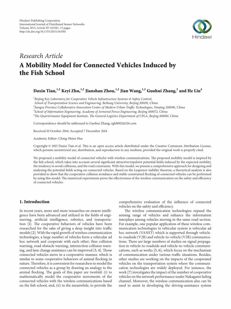
Vehicle i
rWi local warning scope
ri the equivalent radiusdi the range of sensing
Figure 1 The interplay range of vehicle 119894
of the obstacles the constraints of the road and the inter-plays among vehicles in the group including both attractiveand repulsive forces Moreover we assume that vehiclescan communicate with other neighbor vehicles via wirelesscommunication technologies which reflect in sensing rangewhich will be provided later In this paper themain notationsused throughout the paper are given in Notations
In the model each vehicle 119894 belongs to the set of vehiclesdenoted byN = 1 2 119899with the total number of vehicles119899 (119899 gt 2) In a vehicle group we concentrate on the targetvehicle 119894 and its neighbor 119895 forall119894 = 119895 isin N The vectorp119894(119905) = [119909
119894(119905) 119910119894(119905)]119879 signifies the location of vehicle 119894 at time
119905 Besides we describe the force between mobility vehiclesdue to the distance changes among them so that the interplayranges of each vehicle are significant In this paper eachvehicle is treated as a virtual sphere with the radius 119903
119894in
order to correct the drawbacks of overlap (see in Figure 1)The concept of the ldquolocal warning scoperdquo is defined as thelocal circle zonewith radius 119903119882
119894of the vehicle warning that the
situation may be dangerous when other vehicles or obstaclesenter this area In this paper the vehicle can get the informa-tion of the location velocity and other behaviors of neigh-bor vehicles via communicating with other vehicles in itssensing range with the radius as 119889
119894(see in Figure 1)
In order to develop a mobility model which can reflectan accurate traffic situation the model not only considers theinteractive forces among vehicles in the group but also takesthe repulsive forces of obstacles and road boundaries intoaccount These forces are described by a vector at everylocation in the force field Following these considerations wedefined the effects induced by accumulated forces exerted onthe vehicle 119894 as follows
119898119894v119894 (119905) = F(1)
119894(119905) + F(2)
119894(119905) + F(3)
119894(119905) (1)
in which v119894(119905) is the actual velocity at time 119905 of vehicle 119894 with
the mass 119898119894 In formula (1) F(1)
119894(119905) is the attractive force by
the goal of vehicle 119894 F(2)119894(119905) is the interactive force among
connected vehicles and F(3)119894(119905) is the environmental effects of
vehicle 119894 Without special notation the letters in bold rep-resent the term which is a vector within a two-dimensionalplane
Under the effect of the goal the vehicles are expected tomove in the certain direction in the desired speedThereforeF(1)119894(119905) stimulates the vehicle 119894 with a certain desired velocity
V0119894in the expected direction e
119894(119905) Hence the expected veloc-
ity can be formulated as
v119900119894(119905) = V119900
119894e119894 (119905) (2)
However in reality the velocity v119894(119905) at time 119905 of vehicle
may deviate from the desired velocity v0119894(119905) due to the nec-
essary deceleration acceleration or other unknowns ThusF(1)119894(119905) as a stimulus to force the vehicle back to the v0
119894(119905) again
with a relaxation time 120591119894can be given by
F(1)119894(119905) = 119898119894
v119900119894(119905) minus v
119894 (119905)
120591119894
(3)
One of the characteristics of connected vehicles is cooper-ative behaviorThe vehicles benefit from thewireless commu-nication so that they can cooperate in moving as a groupThevehicles aggregate together in the same movement patternwhile keeping the certain safe distance from each other Forthe purpose of formulating the group forces among vehicleswe set the interactive forces into two categories including theattractive force and the repulsive force which can make thevehicles run as a group while keeping a certain distancewithout collisionWe lump the attractive and repulsive forcesin F(2)119894(119905) as follows
F(2)119894(119905) = sum
forall119895isin119873119894(119905)
(F119860119894119895(119905) + F119877
119894119895(119905)) (4)
F(2)119894(119905) is the accumulated forces among target vehicle 119894
and all other neighbor vehicles 119895 in its sensing range F119860119894119895(119905)
is the attractive force on vehicle 119894 from its neighbor vehiclesUnder the influence of the attractive force the vehicles willaccelerate toward each other to keep them as a group Mean-while the F119877
119894119895(119905) is the repulsive force on vehicle 119894 from its
neighbor vehicles to keep the safe distance and to avoidcollisions among connected vehicles
In the short distances like the warning scope the repul-sion is increasing with the decreasing of the distances amongvehicle 119894 and its neighbors Likewise the attraction will play aleading role in making vehicles stay as a group when thedistances among vehicle 119894 and its neighbors are larger thanthe warning scope In the case that the neighbor vehicle isbeyond the bounds of the sensing range 119889
119894 the attraction will
not exist Similarly the repulsive force will not contribute tothe acceleration of a vehicle if it is not in the sensing range ofthe target vehicle In order to depict this situation we use theconcept of potential functions to formularize the attractive
4 International Journal of Distributed Sensor Networks
and repulsive forces Besides according to the research [1922] the potential functions are used to describe the interplaysamong individuals in fish school and vehicles which alsocan control the individual to avoid the obstacle through therepulsive potential field
The effects of two kinds of interplays among vehicles thatis attraction and repulsion are varying along with the chang-ing relative distance between vehicles And the comprehen-sive impact of the interplays can be appropriately modeledwith the potential field functions A bump function model in[28] is adopted to formulate the smooth potential functionswith finite cutoffs In this paper for the sake of simplicity thebump function used to indicate the proximity between thevehicles 119894 and 119895 is denoted by 120593
119894119895(119905) = 120595
119897(p119894(119905) p119895(119905)) By com-
bining 120593119894119895(119905) and the attractiverepulsive potential functions
119880119860(p119894(119905) p119895(119905)) and 119880
119877(p119894(119905) p119895(119905)) the attractiverepulsive
forces are defined as
F119860119894119895(119905) = minus119898119894nabla119880119860 (p119894 (119905) p119895 (119905)) minus 120588119894120593119894119895 (119905) v119894 (119905)
F119877119894119895(119905) = minus119898119894nabla119880119877 (p119894 (119905) p119895 (119905)) minus 120583119894120593119894119895 (119905) v119894 (119905)
(5)
where 120588119894and 120583119894are two positive real coefficients used to scale
the magnitude of the attractiverepulsive forces and they arelimited as 120588
119894 120583119894isin (0 1) in this paper
According to the form of the bump function 120593119894119895(119905) can be
expressed as
120593119894119895 (119905)
=
1 whenΔ119889119894119895 (119905) minus (119903119894 + 119903119895)
119889119894minus (119903119894+ 119903119895)
isin [0 119897]
119896V (1+cos(120587(Δ119889119894119895 (119905)+(119897 minus 1) (119903119894+119903119895)minus119897 times 119889119894
(1 minus 119897) (119889119894 minus (119903119894 + 119903119895))
)))
whenΔ119889119894119895 (119905) minus (119903119894 + 119903119895)
119889119894minus (119903119894+ 119903119895)
isin (119897 1 ]
0 otherwise(6)
where 119896V is similarly a positive parameterwithin (0 1) and thevariable Δ119889
119894119895(119905) denotes the intervehicular distance between
the vehicles 119894 and 119895 at the time 119905 In order to explore theinfluence of the different parameters 119896V and 119897 on the adoptedbump function we conduct the numerical experiment withthe settings of 119889
119894= 300m 119903
119894= 119903119895= 5m 119896V = 02 05 and
119897 = 01 03 05 07 09 The results are shown in Figure 2 Itcan be found that this bump function is a scalar function thatranges between 0 and 1 and has different cutoffs with differentvalues of 119896V and 119897 It also can be seen in Figure 2 that when119896V = 02 and 119897 = 0 the function has a sudden jump at a certainpoint To guarantee the smoothness of the potential functionwe fix 119896
119900= 119896119871= 119896V = 05 and 119897 = 03 in the following
experiments
0 100 200 300 400 500
120593ij(t)
Δdij(t) (m)
k = 02 l = 01k = 05 l = 01
k = 02 l = 03
k = 05 l = 03k = 02 l = 05
k = 05 l = 05
k = 02 l = 07
k = 05 l = 07k = 02 l = 09
k = 05 l = 09
1
09
08
07
06
05
04
03
02
01
0
Figure 2 Bump function with different parameters
The potential function of attractive force is designed asthe form of a tangent function
119880119860(p119894 (119905) p119895 (119905))
=
1
2119896119860tan(
120587 (10038171003817100381710038171003817p119894 (119905) minus p
119895 (119905)10038171003817100381710038171003817minus (119903119894+ 119903119895))
2 (119889119894minus (119903119894+ 119903119895))
)
when 10038171003817100381710038171003817p119894 (119905) minus p119895 (119905)
10038171003817100381710038171003817isin [(119903119894+ 119903119895) 119889119894)
0 otherwise(7)
and the repulsive potential function is given as follows
119880119877(p119894 (119905) p119895 (119905))
=
1
2119896119877(
1
(10038171003817100381710038171003817p119894 (119905) minus p
119895 (119905)10038171003817100381710038171003817minus (119903119894+ 119903119895))2
minus1
(119889119894minus (119903119894+ 119903119895))2)
2
when 10038171003817100381710038171003817p119894 (119905) minus p119895 (119905)
10038171003817100381710038171003817isin ((119903119894+ 119903119895) 119889119894]
0 otherwise(8)
where the vectors p119894= [119909
119894 119910119894]119879 p119895= [119909
119895 119910119895]119879 denote
the position of vehicles 119894 119895 respectively 119896119860and 119896
119877are two
scaling positive real coefficients By introducing the potentialfunctions119880
119860(p119894(119905) p119895(119905)) and119880
119877(p119894(119905) p119895(119905)) we can further
assume that the magnitudes of the attractive and repulsiveeffects existing between two neighboring vehicles 119894 and 119895 areequal when distance Δ119889
119894119895(119905) = p
119894(119905) minus p
119895(119905) between them
International Journal of Distributed Sensor Networks 5
0 50 100 150 200 250 3000
1
2
3
4
5
6UA
kA = 001kA = 005
kA = 01kA = 05
pi(t) minus pj(t) (m)
(a) 119880119860(p119894(119905) p119895(119905)) with different 119896119860
0 50 100 150 200 250 3000
1
2
3
4
5
6
UR
pi(t) minus pj(t) (m)
kR = 120585 times 001
kR = 120585 times 005kR = 120585 times 01kR = 120585 times 05
(b) 119880119877(p119894(119905) p119895(119905)) with different 119896119877
Figure 3 The variation of the potential functions with different parameter settings
stays at a certain desired value Let this desired distance beΔ119889desire isin ((119903119894 + 119903119895) 119889119894) Note that the attractive and repulsiveeffects are represented by the gradients of the potentialfunctions119880
119860(p119894(119905) p119895(119905)) and 119880
119877(p119894(119905) p119895(119905)) with respect to
the relative distance between the vehicles 119894 and 119895 respec-tively Accordingly 119896
119860and 119896
119877should be set to satisfy the
partial differential equation 120597119880119860(p119894(119905) p119895(119905))120597Δ119889
119894119895(119905) =
120597119880119877(p119894(119905) p119895(119905))120597Δ119889
119894119895(119905) under the condition of Δ119889
119894119895(119905) =
Δ119889desire By substituting Δ119889119894119895(119905) = Δ119889desire into (7) and (8)
and solving the equation 120597119880119860(p119894(119905) p119895(119905))120597Δ119889
119894119895(119905) =
120597119880119877(p119894(119905) p119895(119905))120597Δ119889
119894119895(119905) we can get the relationship of the
magnitudes of 119896119860and 119896119877as follows
119896119877
119896119860
= (120587
4 (119889119894minus (119903119894+ 119903119895))
times(cosminus2(1205872(
Δ119889desire minus (119903119894 + 119903119895)
119889119894minus (119903119894+ 119903119895)
))))
times (2 (Δ119889desire minus (119903119894 + 119903119895))minus3
times [(Δ119889desire minus (119903119894 + 119903119895))minus2
minus (119889119894minus (119903119894+ 119903119895))minus2
])
minus1
(9)
Based on (9) it can be seen that once the desired distanceΔ119889desire among vehicles and the parameters 119889
119894 119903119894 and 119903
119895are
given the settings on 119896119860and 119896
119877are expected to satisfy the
relationship 119896119877= 120585 times 119896
119860where 120585 is set to be the result of the
right side of (9) In order to explore the impact of the param-eters 119903
119894and 119903119895on the potential functions 119880
119860(p119894(119905) p119895(119905)) and
119880119877(p119894(119905) p119895(119905)) we conduct the following numerical experi-
ment where the sensing range 119889119894is fixed at 300m and 119903
119894has
the same value with 119903119895for simplicity that is 119903
119894= 119903119895= 5m In
addition the desired distanceΔ119889desire is set to be 50m and theparameter 119896
119860discretely varies from 001 to 05 According to
(9) the ratio of 119896119877and 119896119860can be calculated as 120585 = 1482times105
Hence in this experiment we can set the other parameter 119896119877
as 119896119877= 120585 times 119896
119860= 1482times10
5119896119860 The relevant results are given
in Figure 3FromFigure 3 it can be found that the potential functions
are both monotonously varying along with the value ofthe distance p
119894(119905) minus p
119895(119905) between vehicle 119894 and vehi-
cle 119895 The definitions of the functions 119880119860(p119894(119905) p119895(119905)) and
119880119877(p119894(119905) p119895(119905)) guarantee that the attractive and repulsive
potential fields have the important properties respectivelythe smaller the distance p
119894(119905)minusp
119895(119905) is the smaller the effect
of the attractive potential field becomes while the effect of therepulsive potential field is increasing along with decreasingthe distance p
119894(119905) minus p
119895(119905) As shown in Figure 3 when
p119894(119905) minus p
119895(119905) decreasingly approaches the value of (119903
119894+ 119903119895)
119880119860(p119894(119905) p119895(119905)) is reduced to zero while 119880
119877(p119894(119905) p119895(119905)) dra-
matically increases This indicates that when a vehicle tendsto collide with another vehicle the attractive potential effectshould be weakened and the repulsive effect strengthenedat the same time Hence the comprehensive effect resultingfrom both the attractive and repulsive potential fields willforce the vehicle to avoid the collisions Additionally fromFigure 3 it can be found that the larger the parameters119896119877and 119896
119860are the steeper the slopes of 119880
119860(p119894(119905) p119895(119905))
and 119880119877(p119894(119905) p119895(119905)) become At this point large parameter
settings on 119896119877and 119896
119860would make the potential fields more
sensitive to the time-related change in the intervehiculardistance Hence an appropriate value of 119896
119877and 119896
119860should
be chosen carefully According to the results presented by
6 International Journal of Distributed Sensor Networks
Figure 3 we fix 119896119860= 01 and 119896
119877= 120585 times 119896
119860for ourmodel in the
other following experiments for the sake of controlling thesensitivity of the potential field functions119880
119860(p119894(119905) p119895(119905)) and
119880119877(p119894(119905) p119895(119905))
On the other side some other environmental factorsinfluencing the movement of the connected vehicles shouldbe taken into account as well such as the road obstacles andthe road constraints That is the vehicles on the road mightface the obstacles like accidents road maintenances andother emergencies Besides the vehicles are also constrainedby the road boundaries which is different from the fishschool In this work the effects arising from road obstaclesand road boundaries are modeled as
F(3)119894(119905) = sum
forall119896isin119872
F119900119894119896(119905) + F119871
119894(119905) (10)
where F119900119894119896(119905) is the repulsive forces of the obstacle 119896 119896 =
1 2 119872 (119872 is the amount of the road obstacles) and F119871119894(119905)
is the virtual repulsive force that forces a vehicle to be awayfrom the boundary of the road and to stay within the roadwhen the vehicle is too close to one boundary and woulddrive off the road Since the decrease in the relative distancebetween a vehicle and an obstacle or between a vehicle andone road boundary would lead to the increase in the repulsiveeffect on the vehicle the repulsive forces of road obstacles androad boundaries should be formulated as decreasing func-tions of such a relative distance By referring to the bumpfunction given in (6) we propose the potential field functionsto model the repulsive effect arising from road obstacles androad boundaries as follows
Define the vector p119874119896= [119909119874
119896(119905) 119910119874
119896(119905)]119879 as the position of
a certain obstacle denoted by 119874119896 The obstacle in this paper
is treated as a ball with the radius 119903119900119896 When the vehicle 119894
approaches to the obstacle 119874119896in proximity and the distance
p119894(119905) minus p119874
119896 becomes smaller than the sensing range 119889
119894
the vehicle 119894will detect it and prepare for avoiding it Further-more F119900
119894119896(119905) should be a monotonically decreasing function
of the distance between the obstacle119874119896and the vehicle 119894 in the
sensing range and the vehicle 119894 should keep a certain distancefrom the obstacles so as to avoid the collision Then thefunction of the repulsive force induced by a bump functiondefined in [28] is designed as
F119900119894119896(119905) = 119865
119900
119894119896times 120593119897(p119894 (119905) p
119900
119896(119905))n119894119896 (119905) (11)
where 119865119900119894119896is the maximum magnitude of the obstacle repul-
sive force F119900119894119896(119905) which is a scalar and n
119894119896(119905) is a unit vector
used to indicate the repulsive acting direction at the timeinstant 119905
n119894119896 (119905) =
(p119894 (119905) minus p119900
119896(119905))
1003817100381710038171003817p119894 (119905) minus p119900119896(119905)1003817100381710038171003817
(12)
and the bump function 120593119897(p119894(119905) p119900119896(119905)) is represented as
120593119897(p119894 (119905) p119900119896 (119905))
=
1 whenΔ119889119894119896 (119905) minus (119903119894 + 119903
119900
119896)
119889119894minus (119903119894+ 119903119900
119896)
isin [0 119897]
119896119900(1+cos(120587(
Δ119889119894119896 (119905)+(119897minus1) (119903119894+119903
119900
119896)minus119897times119889
119894
(1 minus 119897) (119889119894 minus (119903119894 + 119903119900
119896))
)))
whenΔ119889119894119896 (119905) minus (119903119894 + 119903
119900
119896)
119889119894minus (119903119894+ 119903119900
119896)
isin (119897 1]
0 otherwise(13)
where Δ119889119894119896(119905) = p
119894(119905) minus p119900
119896(119905) and 119896
119900and 119897 are positive real
coefficients whose values are limited within (0 1)Considering the constraints of road is essential for real-
istic modeling of connected vehicles moving as a group theroad constraints force which is similar to the force of theobstacle is defined as
F119871119894(119905) = 119865
119871
119894120595119897(p119894 (119905) p
119871
119894(119905))n119871119894(119905) (14)
where 119865119871119894is the maximum magnitude of the force F119871
119894(119905) and
120595119897(p119894(119905) p119871119894(119905)) is also designed as a bump function as follows
120595119897(p119894 (119905) p
119871
119894(119905))
=
1 whenΔ119889119871
119894(119905) minus 119903119894
119877 minus 119903119894
isin [0 119897]
119896119871(1 + cos(120587(
Δ119889119871
119894(119905) + (119897 minus 1) 119903119894 minus 119897 times 119877
(1 minus 119897) (119877 minus 119903119894))))
whenΔ119889119871
119894(119905) minus 119903119894
119877 minus 119903119894
isin (119897 1]
0 otherwise(15)
where 119896119871isin (0 1) and p119871
119894(119905) represents the position of the
vehicle 119894rsquos center projection point on the nearest road bound-ary line at the time instant 119905 and Δ119889119871
119894(119905) = p
119894(119905) minus p119871
119894(119905)
n119871119894(119905) is the unit direction vector from p119871
119894(119905) to p
119894(119905) that
is perpendicular to the road boundary line which can becalculated as
n119871119894(119905) =
p119894 (119905) minus p119871
119894(119905)
Δ119889119871
119894(119905)
(16)
The parameter 119877 is the maximum range of the virtual roadconstraint force acting on a vehicle From the equation aboveit can be seen that when the relative distance between thevehicle 119894 and its nearest road boundary (ie Δ119889119871
119894(119905)) is larger
than119877 this virtual road constraint force is set to 0 otherwisethe closer to the road boundary the vehicle is the larger thisrepulsive force becomes
In addition in order to make the repulsive forces F119900119894119896(119905)
and F119871119894(119905) respectively induced by the obstacles and the road
constraints dynamically coordinated with the attractive force
International Journal of Distributed Sensor Networks 7
arising from the desired velocity v119900119894(119905) we combine them
with F(1)119894(119905) defined in (3) and then defined the maximum
magnitudes of these two repulsive forces as follows
119865119900
119894119896(119905) = 120574119894119896 times
10038161003816100381610038161003816F(1)119894(119905) sdot n119894119896 (119905)
10038161003816100381610038161003816
= 120574119894119896
119898119894
120591119894
1003816100381610038161003816(v119900
119894(119905) minus v
119894 (119905)) sdot n119894119896 (119905)1003816100381610038161003816
119865119871
119894(119905) = 120573119894 times
10038161003816100381610038161003816F(1)119894(119905) sdot n119871
119894(119905)10038161003816100381610038161003816
= 120573119894
119898119894
120591119894
10038161003816100381610038161003816(v119900119894(119905) minus v
119894 (119905)) sdot n119871
119894(119905)10038161003816100381610038161003816
(17)
where |lowast| is the absolute value sign and 120574119894119896and 120573
119894are positive
sensitivity coefficients within (0 1] which are used to scaleand coordinate the magnitudes of 119865119900
119894119896(119905) and 119865119871
119894(119905)
22 Stability Analysis of Connected Vehicles Since connectedvehicles are equipped with wireless communications one isable to interact with the others in its sensing range Thusthese mobile terminals constitute a local vehicular networkThe communication topology of these connected vehiclesat any time instant 119905 can be presented by a bidirectionalgraph which can also be called as communication graphLet 119866(119905) = (119881 119864(119905)) denote this communication graph and119881 = 119894 | forall119894 isin N As aforementioned in Section 21 weassume that the sensing range of all the vehicles is identicalthat is 119889
119894= 119889 (forall119894 isin 119881) Subsequently an edge in this
communication graph 119866(119905) is used to indicate a bidirectionalwireless communication interaction between a vehicle andonemember in this vehiclersquos neighborThat is the set of thoseedges in119866(119905) can be defined as119864(119905) = (119894 119895) | p
119894(119905)minusp
119895(119905) lt
119889 and 119864(119905) isin 119881 times 119881 For simplicity we also denote theneighboring nodes of any node 119894 (ie the vehicle 119894) in thegiven communication graph119866(119905) at any time instant 119905 as a set119873119894(119905) = 119895 | (119894 119895) isin 119864(119905) 119895 isin 119881 From the notation of 119864(119905)
it is obviously seen that the topology of this communicationgraph is varying over time due to the possibility of a vehicleentering into or out of the communication range of a hostvehicle Attempting to analyze the overall mobility of a givenvehicle group moving in the same road we assume that theinitial velocity of all those vehicles is the same and theirdesired velocities at any time instant 119905 are also identical thatis v119894(0) = v and v119900
119894(119905) = v119900(119905) for all vehicles 119894 isin 119881
It should be noted that this assumption is reasonable sincevehicles would move with a constant velocity in the samedirection when they are in an equilibrium traffic flow of thesame road and encounter no emergencies or disturbancesAlso we assume that the sensing ranges of all the vehicles areequal that is 119889
119894= 119889119895for forall119894 = 119895 isin 119881 We introduce
the concept of the ldquogroup centroidrdquo which is represented asp119888(119905) = (1119873) times sum
119873
119894=1p119894(119905) Now we state the analysis results
of our proposed mobility model
Corollary 1 Consider that connected vehicles with wirelesscommunications evolve under the mobility model defined by(1) and given that sum
forall119896isin119872120574119894119896+ 120573119894le 1 v
119894(0) = v and v119900
119894(119905) =
v119900(119905) for all vehicles 119894 isin 119881 the overall group can asymptoticallyconverge to the desired velocity v119900(119905) which is defined in (2)
Proof We can lump all the forces of every vehicle as follows
sum
forall119894isin119881
119898119894v119894 (119905) = sum
forall119894isin119881
(F(1)119894(119905) + F(2)
119894(119905) + F(3)
119894(119905)) (18)
Since the condition is given that 119889119894= 119889119895for forall119894 = 119895 isin 119881 and
these forces F119860119894119895(119905) and F119877
119894119895(119905) are bidirectional for all vehicles
119894 isin 119881 we have F119860119894119895(119905) = minusF119860
119895119894(119905) and F119877
119894119895(119905) = minusF119877
119895119894(119905) according
to (5) At this point we further have
sum
forall119894isin119881
F(2)119894(119905) = sum
forall119894isin119881
( sum
forall119895isin119873119894(119905)
(F119860119894119895(119905) + F119877
119894119895(119905)))
= sum
forall119894 =119895isin119881
forall(119894119895)isin119864(119905)
(F119860119894119895(119905) + F119877
119894119895(119905) + F119860
119895119894(119905) + F119877
119895119894(119905)) = 0
(19)
Therefore equation (1) can be rearranged as sumforall119894isin119881
119898119894v119894(119905) =
sumforall119894isin119881
(F(1)119894(119905) + F(3)
119894(119905)) Now recalling that the bump func-
tions 120593119897(p119894(119905) p119900119896(119905)) and 120593
119897(p119894(119905) p119871119894(119905)) are limited within
[0 1] we can get the inequality as follows10038171003817100381710038171003817F(3)119894(119905)10038171003817100381710038171003817
=
1003817100381710038171003817100381710038171003817100381710038171003817
( sum
forall119896isin119872
119865119900
119894119896(119905) times 120593119897 (p119894 (119905) p
119900
119896(119905))n119894119896 (119905))
+ 119865119871
119894(119905) 120595119897 (p119894 (119905) p
119871
119896(119905))n119871119894(119905)
1003817100381710038171003817100381710038171003817100381710038171003817
le
1003817100381710038171003817100381710038171003817100381710038171003817
( sum
forall119896isin119872
119865119900
119894119896(119905) times 120593119897 (p119894 (119905) p
119900
119896(119905))n119894119896 (119905))
1003817100381710038171003817100381710038171003817100381710038171003817
+10038171003817100381710038171003817119865119871
119894(119905) 120595119897 (p119894 (119905) p
119871
119896(119905))n119871119894(119905)10038171003817100381710038171003817
le sum
forall119896isin119872
119865119900
119894119896(119905) + 119865
119871
119894(119905)
= sum
forall119896isin119872
120574119894119896
119898119894
120591119894
1003816100381610038161003816(v119900
119894(119905) minus v
119894 (119905)) sdot n119894119896 (119905)1003816100381610038161003816
+ 120573119894
119898119894
120591119894
10038161003816100381610038161003816(v119900119894(119905) minus v
119894 (119905)) sdot n119871
119894(119905)10038161003816100381610038161003816
le sum
forall119896isin119872
120574119894119896
119898119894
120591119894
1003817100381710038171003817v119900
119894(119905) minus v
119894 (119905)1003817100381710038171003817 + 120573119894
119898119894
120591119894
1003817100381710038171003817v119900
119894(119905) minus v
119894 (119905)1003817100381710038171003817
= ( sum
forall119896isin119872
120574119894119896+ 120573119894)119898119894
120591119894
1003817100381710038171003817v119900
119894(119905) minus v
119894 (119905)1003817100381710038171003817 le
10038171003817100381710038171003817F(1)119894(119905)10038171003817100381710038171003817
(20)
Hence the magnitude of the attractive force induced by thedesired velocity v119900
119894(119905) is larger than that of the force induced
by the obstacle and the road boundary This implies that themobility of the overall vehicle group is mainly dominated bythe potential field that can force vehicles to keepmoving withor asymptotically converge to the desired velocity even afterbeing disturbed by the repulsive potentials resulting from
8 International Journal of Distributed Sensor Networks
obstacles and road constraints At this point we proveCorollary 1
Now we firstly provide some properties of the potentialfunctions 119880
119860(p119894(119905) p119895(119905)) and 119880
119877(p119894(119905) p119895(119905)) related to the
interactive force F(2)119894(119905) as follows For simplicity we
equivalently denote 119880119860(Δ119889119894119895(119905)) = 119880
119860(p119894(119905) p119895(119905)) and
119880119877(Δ119889119894119895(119905)) = 119880
119877(p119894(119905) p119895(119905)) whereΔ119889
119894119895(119905) = p
119894(119905)minusp
119895(119905)
The following can be mathematically proven
Corollary 2 119880119860(Δ119889119894119895(119905)) satisfies the following properties (i)
it is continuously differentiable for Δ119889119894119895(119905) isin [(119903
119894+ 119903119895) 119889119894)
and is a monotonously increasing function of Δ119889119894119895(119905) within
[(119903119894+ 119903119895) 119889119894) that makes 119880
119860(Δ119889119894119895(119905)) rarr 0 with Δ119889
119894119895(119905) rarr
(119903119894+ 119903119895) and 119880
119860(Δ119889119894119895(119905)) rarr infin with Δ119889
119894119895(119905) rarr 119889
119894
(ii) 119906119860119894119895= 119906119860
119895119894when denoting 119906119860
119894119895= 120597119880
119860(Δ119889119894119895(119905))120597Δ119889
119894119895(119905)
for forall(119894 119895) isin 119864(119905) and (iii) sumforall(119894119895)isin119864(119905)
(120597119880119860(Δ119889119894119895(119905))120597p
119894(119905)) =
sumforall119894 =119895isin119881
(120597119880119860(Δ119889119894119895(119905))120597p
119894(119905))
Proof It is easily obtained that the partial derivative of119880119860(Δ119889119894119895(119905)) with respect to Δ119889
119894119895(119905) is expressed as
119906119860
119894119895=
120597119880119860(Δ119889119894119895 (119905))
120597Δ119889119894119895 (119905)
=120587
4 (119889119894minus (119903119894+ 119903119895))
times 119896119860(cos(
120587 (Δ119889119894119895 (119905) minus (119903119894 + 119903119895))
2 (119889119894minus (119903119894+ 119903119895))
))
minus2
gt 0
(21)
for Δ119889119894119895(119905) isin [(119903
119894+ 119903119895) 119889119894) At this point 119880
119860(Δ119889119894119895(119905)) is a
monotonously increasing function that is defined on [(119903119894+
119903119895) 119889119894) Consequently we further get
limΔ119889119894119895(119905)rarr (119903119894+119903119895)
119880119860(Δ119889119894119895 (119905)) = 119880119860 ((119903119894 + 119903119895)) = 0
limΔ119889119894119895(119905)rarr119889119894
119880119860(Δ119889119894119895 (119905)) = 119880119860 (119889119894) = infin
(22)
and 119906119860119894119895gt 0 for Δ119889
119894119895(119905) isin ((119903
119894+ 119903119895) 119889119894) Thus property (i) is
proven Moreover recall that we have assumed 119889119894= 119889119895for
forall119894 = 119895 isin 119881 This means that the sensing ability (sensingrange) of every vehicle is identical Hence according toΔ119889119894119895(119905) = Δ119889
119895119894(119905) it can be seen that 120597119880
119860(Δ119889119894119895(119905))120597Δ119889
119894119895(119905) =
120597119880119860(Δ119889119895119894(119905))120597Δ119889
119895119894(119905) that is 119906119860
119894119895= 119906119860
119895119894 Thus property (ii)
is proven Noting the definition of 119880119860(Δ119889119894119895(119905)) and the
communication graph 119866(119905) when one vehicle 119895 is not in theneighbor 119873
119894(119905) of another vehicle 119894 the relative distance
between them Δ119889119894119895(119905) is larger than the sensing range 119889
119894
Then the potential119880119860(Δ119889119894119895(119905)) is set to 0 accordingly as well
as 120597119880119860(Δ119889119894119895(119905))120597Δ119889
119894119895(119905) = 0 So we have
sum
forall119894 =119895isin119881
120597119880119860(Δ119889119894119895 (119905))
120597p119894 (119905)
= sum
forall119895isin119881119873119894(119905)
120597119880119860(Δ119889119894119895 (119905))
120597p119894 (119905)
+ sum
forall119895isin119873119894(119905)
120597119880119860(Δ119889119894119895 (119905))
120597p119894 (119905)
= 0 + sum
forall119895isin119873119894(119905)
120597119880119860(Δ119889119894119895 (119905))
120597p119894 (119905)
= sum
forall(119894119895)isin119864(119905)
120597119880119860(Δ119889119894119895 (119905))
120597p119894 (119905)
(23)
This finishes the proof of property (iii)
Similarly we present Corollary 3 for the potential func-tion 119880
119877(Δ119889119894119895(119905)) Its proof can also be finished in the similar
way of proving Corollary 2 so it is not needed to repeat themhere in consideration of space
Corollary 3 119880119877(Δ119889119894119895(119905)) is (i) continuously differentiable
for Δ119889119894119895(119905) isin ((119903
119894+ 119903119895) 119889119894] while it is a monotonously
decreasing function defined on ((119903119894+ 119903119895) 119889119894] that satisfies
119880119877(Δ119889119894119895(119905)) rarr infin with Δ119889
119894119895(119905) rarr (119903
119894+ 119903119895) and
119880119877(Δ119889119894119895(119905)) rarr 0withΔ119889
119894119895(119905) rarr 119889
119894 (ii) the partial derivative
119906119877
119894119895= 120597119880119877(Δ119889119894119895(119905))120597Δ119889
119894119895(119905) (119906119877119894119895lt 0) also satisfies the sym-
metry119906119877119894119895= 119906119877
119895119894forforall(119894 119895) isin 119864(119905) and (iii) sum
forall(119894119895)isin119864(119905)(120597119880119877(Δ119889119894119895
(119905))120597p119894(119905)) = sum
forall119894 =119895isin119881(120597119880119877(Δ119889119894119895(119905))120597p
119894(119905))
In addition it is significant to analyze the intragroupmobility besides the basic characteristic of the overall groupFrom model (1) it can be noted that the connected vehi-cle group model can be decomposed into two terms theattractiverepulsive forces induced by the external potentialsincluding F(1)
119894(119905) and F(3)
119894(119905) and the interactive force F(2)
119894(119905)
that exists among vehicles According to the principle of inertialframe of reference when the group centroid p
119888(119905) is set as an
original point of the inertial frame of reference each vehiclersquosmotion relative to this reference frame is mainly dependent onthe interactive force F(2)
119894(119905) induced by the attractiverepulsive
potentials between vehicles instead of the external force poten-tials F(1)
119894(119905) and F(3)
119894(119905)Thus in order to analyze the intragroup
mobility we turn to focus on the influence of the interactiveforce F(2)
119894(119905) between vehicles Then the derivative of a vehiclersquos
velocity relative to the reference frame (the relative velocity isdenoted by v119888
119894(119905)) with respect to the time instant 119905 can be
expressed as
119898119894v119888119894(119905) = F(2)
119894(119905) (24)
Also let p119888119894(119905) be the relative position of the vehicle 119894 in the
reference frame The vehicle dynamic system in the referenceframe is then formulated as follows
p119888119894(119905) = v119888
119894(119905)
v119888119894(119905) =
1
119898119894
F(2)119894(119905)
= minus sum
forall119894 =119895isin119881
nabla119880119860(Δ119889119894119895 (119905)) + nabla119880119877 (Δ119889119894119895 (119905))
minus sum
forall119894 =119895isin119881
(120588119894+ 120583119894)
119898119894
120593119894119895 (119905) v
119888
119894(119905)
(25)
Based on the vehicle dynamic systemmodel above one formof the Lyapunov function 119871(119905) for the whole group can be
International Journal of Distributed Sensor Networks 9
designed by combining the potential field energy and thekinematic energy as
119871 (119905) = 119880 (119905) + 119881 (119905) (26)
where the potential field term is 119880(119905) = sumforall119894isin119881
sumforall(119894119895)isin119864(119905)
(119880119860(Δ119889119894119895(119905))+119880
119877(Δ119889119894119895(119905))) and the kinematic energy is119881(119905) =
(12)sumforall119894isin119881
v119888119894(119905)2 Thus by differentiating 119871(119905) with respect
to the time variable 119905 one further gets
(119905)
= sum
forall119894isin119881
sum
forall(119894119895)isin119864(119905)
(nabla119880119860(Δ119889119894119895 (119905)) + nabla119880119877 (Δ119889119894119895 (119905)))
119879
sdot p119888119894(119905) + sum
forall119894isin119881
(v119888119894(119905))119879sdot v119888119894(119905)
= sum
forall119894isin119881
sum
forall(119894119895)isin119864(119905)
(nabla119880119860(Δ119889119894119895 (119905)) + nabla119880119877 (Δ119889119894119895 (119905)))
119879
sdot v119888119894(119905)
+ sum
forall119894isin119881
(v119888119894(119905))119879
sdot (minus sum
forall119894 =119895isin119881
nabla119880119860(Δ119889119894119895 (119905)) + nabla119880119877 (Δ119889119894119895 (119905))
minus sum
forall119894 =119895isin119881
(120588119894+ 120583119894)
119898119894
120593119894119895 (119905) v
119888
119894(119905))
(27)
According to Corollaries 2 and 3 it should be noted that
sum
forall(119894119895)isin119864(119905)
(nabla119880119860(Δ119889119894119895 (119905)))
119879
sdot v119888119894(119905)
minus sum
forall119894 =119895isin119881
[(v119888119894(119905))119879sdot nabla119880119860(Δ119889119894119895 (119905))] = 0
sum
forall(119894119895)isin119864(119905)
(nabla119880119877(Δ119889119894119895 (119905)))
119879
sdot v119888119894(119905)
minus sum
forall119894 =119895isin119881
[(v119888119894(119905))119879sdot nabla119880119877(Δ119889119894119895 (119905))] = 0
(28)
Therefore (119905) = minussumforall119894isin119881
sumforall119894 =119895isin119881
((120588119894+ 120583119894)119898119894)120593119894119895(119905)
(v119888119894(119905))119879sdot v119888119894(119905) Since (v119888
119894(119905))119879sdot v119888119894(119905) ge 0 and ((120588
119894+ 120583119894)
119898119894)120593119894119895(119905) ge 0 we have (119905) le 0 which means that those
vehicles in the reference frame can asymptotically converge toa stable state In the actual reference frame this fact suggeststhat those vehicles having knowledge of some other vehiclesrsquostate in their local neighbor tend to move as an overall groupNow based on this we declare the following result to illustratethe potential of collision avoidance among vehicles equippedwith wireless communications
Theorem 4 Consider that connected vehicles with wirelesscommunications evolve under mobility model (1) and giventhat sum
forall119896isin119872120574119894119896+ 120573119894le 1 v
119894(0) = v and v119900
119894(119905) = v119900(119905) for all
vehicles 119894 isin 119881 If Δ119889119894119895(0) gt (119903
119894+ 119903119895) for forall119894 = 119895 isin 119881 those
vehicles move as an overall group that tends to keep avoidingintrasystem collision
Proof According to Corollary 1 those vehicles tend to keepthe same desired velocity v119900(119905) Furthermore since we have(119905) le 0 for 119905 ge 0 119871(119905) le 119871(0) lt infin If there were at leasttwo vehicles 119894 and 119895 extending to collide with each other thatis Δ119889
119894119895(119905) rarr (119903
119894+ 119903119895) 119871(119905) = (119880(119905) + 119881(119905)) rarr infin due to
119880(119905) rarr infin under the consideration of the property (i) inCorollary 3 Hence the contradiction occurs At this pointany two vehicles 119894 and 119895 in the group do not extend to collidewith each other That is this theorem is proven
Theorem 5 Consider that connected vehicles with wirelesscommunications evolve under mobility model (1) given thatsumforall119896isin119872
120574119894119896+ 120573119894le 1 v
119894(0) = v and v119900
119894(119905) = v119900(119905) for all vehicles
119894 isin 119881 Those vehicles that initially belong to the neighboringmember of one certain vehicle 119894 that is those ones (119894 119895) isin 119864(0)(forall119894 isin 119881) tend to keep connecting to this vehicle 119894 when allvehicles move as an overall group
Proof Similar to the proof of Theorem 4 since (119905) le 0 for119905 ge 0 119871(119905) le 119871(0) lt infin Recall property (i) in Corollary 2When any one neighboring member 119895 of a vehicle 119894 tends tomove out of the sensing range that is Δ119889
119894119895(119905) rarr 119889
119894((119894 119895) isin
119864(0)) 119880119860(Δ119889119894119895(119905)) rarr infin so that 119880(119905) rarr infin Hence 119871(119905) =
(119880(119905) + 119881(119905)) rarr infin when at least one pair (119894 119895) is satisfyingΔ119889119894119895(119905) rarr 119889
119894 This is contradictory to the fact that (119905) le 0
for 119905 ge 0 In this way we proveTheorem 5
3 Simulations
In this section simulations achieved by MATLAB are pro-vided to verify the model proposed in previous section Theanalysis of the results is also given in this section in orderto characterize the benefit of wireless communication amongvehicles for safety and efficiency of traffic We set up a trafficscene where an accident situation on the unidirectional roadas the obstacle has to be avoided Then we get the diagramof the trajectories of the connected vehicles to demonstratethat the model can achieve the obstacle avoidance effectivelyIn addition we also have the comparative numerical experi-ment of vehicles with wireless communications and withoutwireless communications while travelling which characterizethe impacts of the communications in the connected vehicles
The simulation scene is assumed on a section of a uni-directional road The unidirectional road we concentrate onis 2000 meters long and 50 meters wide We suppose that anaccident occurs on the road where the location of the centerof it is marked as 119874
1 The obstacle is a circle region with the
center set to be 1000 meters away from the beginning bound-ary of the simulation range and with radius of 119903119874
119894= 5meters
which needed to be detoured Namely a collision will occurwhen the vehicle enters the circle area
10 International Journal of Distributed Sensor Networks
980 990 1000 1010 10200
5
10
15
20
25
30
35
40
45
50
(a) Average velocity V = 10ms
980 990 1000 1010 10200
5
10
15
20
25
30
35
40
45
50
(b) Average velocity V = 15ms
980 990 1000 1010 10200
5
10
15
20
25
30
35
40
45
50
(c) Average velocity V = 20ms
Figure 4 The travelling trajectory of vehicles
The number and the velocity of vehicles are producedrandomly at the start of simulations During the simulationsthose connected vehicles are controlled by our proposedmodel to move as a cooperative group whose direction isconsistent In all simulations we fix the time interval forupdating the kinematic information of each vehicle at 01 sBesides the physical parameters of the vehicle are given as119903119894= 5m 119889
119894= 300m 119898
119894= 2000 kg and 119903119882
119894= 7m More-
over other parameters required in the simulations are set asΔ119889desire = 50m 120591
119894= 005 s 120588
119894= 01 120583
119894= 01 119896V = 05
119896119860= 01 119896
119877= 1482 times 105119896
119860 119896119874= 05 119897 = 03 119896
119871= 05
119877 = 3m 120574119894119896= 08 (119896 = 1 and forall119894 isin 119881) and 120573
119894= 06
31 Obstacle Avoidance Trajectory Figure 4 shows the vari-ous travelling trajectories of each vehicle when the vehiclegroup comes across the obstacle in different average veloc-ities In these simulations the average velocities are set to10ms 15ms and 20ms separately in order to explore theperformances of avoiding obstacles in different velocitiesWhat is more the total number of vehicles is the samein these three simulations set as 119899 = 20 The axes inFigures 4(a) 4(b) and 4(c) are the referenced coordinatesused to measure the real-time position of vehicles movingon the road whose unit is meter From Figure 4 it can beobserved that when encountering the obstacle the vehicles
International Journal of Distributed Sensor Networks 11
change into two subgroups like the behaviors of fish schoolwhen the established information is locally broadcasted inthe whole group Subsequently they are unified into a groupagain as before after successfully avoiding this obstacle Inaddition comparing the travelling trajectory in differentaverage velocities the conclusion can be drawn that the lowerthe average velocity of vehicles is the easier the vehiclesunified together Although various velocities have differenttravelling trajectory all the vehicles have been successfullyreached and the vehicles have stayed together as a group andavoided collisions or obstacles This result indicates that themodel of connected vehicles based on the behaviors of fishschool is effective in describing the cooperative behaviors inavoiding obstacles
32 Impacts of Wireless Communications In order to explorethe influences of wireless communications on the overallmobility of connected vehicles we also conduct other com-parative numerical experiments In the simulationswhen anyvehicle 119894 is considered to be equipped with wireless commu-nications its sensing range is set to 119889
119894= 300m otherwise
the sensing range of a driver is limited to 119889119894= 100m
if the relevant vehicle 119894 is not equipped with wireless com-munications and its driving decision is made dependent onvisual perception Thus those experiment results shown inthe following figures marked by ldquoEquippedrdquo are related tothe specific case where every vehicle is considered to be ableto communicate with its neighbors via wireless communica-tions while the results marked by ldquoUnequippedrdquo are obtainedin the other case where all of the vehicles can only interactwith others in the aforementioned shorter sensing range Forcomparison the following performance metrics are defined
(i) Probability of a Vehicle Moving into the Local WarningScope of Obstacle 119875
119900 Recalling that we assume there is an
obstacle with the radius of 5mon the road it should be notedthat even though a vehicle can successfully avoid collidingwith the obstacle its situation may be dangerous when it istoo close to this obstacle Thus the probability of an obstacleentering into the predefined local warning scope of thevehicle 119894 can be used to quantify the danger severity evenwhen there are not any obstacle collisions occurring
(ii) Probability of a Vehicle Moving into the Local WarningScope of Other Vehicles 119875V Similarly the local warning scopeof a vehicle is defined as the local range with a radius of 7mthat covers this vehicleWith thismetric we can also quantifythe danger severity of vehicles equipped with or withoutwireless communications as moving even when no vehiclecollisions occur among them
Subsequently let Event(119896) represent the total number ofthe events occurring at the 119896th simulation epoch in which theobstacle or other vehicles enter into the local warning scopeof vehicle 119894 let 119873 = |N| be the total number of vehiclesand TotalEpoch the total number of simulation epochsThesemetrics 119875
119900and 119875V are calculated as follows
119875119900or 119875V =
sumTotalEpoch119896=1
Event (119896)TotalEpoch times 119873
(29)
In a real life traffic situation the vehicle velocity willsignificantly affect the mobility of the overall vehicle groupIn addition it is necessary to evaluate the traffic efficiencyof connected vehicles flocking as a group under differentvehicle numbers (indicating the traffic density) Therefore inthis paper the impacts of the wireless communications ofconnected vehicles by varying vehicle velocity and vehiclenumber are studied
To analyze the impacts on road safety level firstly we varythe initial vehicle velocity from 10ms to 30ms and fix thetotal number of vehicles at 119873 = 30 At each vehicle velocitypoint simulation has been performed 30 times repeatedlyand the metrics 119875
119900and 119875V are then averaged Additionally
the standard deviations of these evaluation metrics are alsocalculated at each velocity The relevant results are shownin Figure 5 As can be seen from these results the dangerseverity indicated by 119875
119900 119875V increases with increasing vehicle
velocity Because the higher the velocity a vehicle moveswith on the road the more the time this vehicle needs todecelerate to a certain lower velocity and the larger thepossibility of the obstacle or other vehicles entering intothe predefined local warning scope of vehicle 119894 the dangerseverity on the road indicated by 119875
119900and 119875V is higher with
higher vehicularmobility Nevertheless assistedwithwirelesscommunications connected vehicles are able to make a deci-sion on braking in advance and larger distance is reserved forchanging their motion trajectory Therefore the metrics 119875
119900
and 119875V obtained in the case marked by ldquoEquippedrdquo are loweron the overall level than those in the ldquoUnequippedrdquo case InFigure 5(b) especially 119875V in the ldquoEquippedrdquo case is reduced by5789 on average compared with that in the ldquoUnequippedrdquocase when the vehicle velocity is larger than 10ms Hencethis suggests that vehicles can benefit from wireless com-munications in terms of extending the perception range andenhancing traffic safety level
Next we turn to focus on the effects of different vehiclenumbers of the group on the safety level For comparisonthe following experiment is processed by varying the vehiclenumber from 10 to 70 and fixing the initial vehicle velocityat 20ms Also the simulations have been performed with30 replications per vehicle number and subsequently theresults of 119875
119900and 119875V obtained at each vehicle number are
averagedThe error bars in Figure 6 also indicate the standarddeviations of 119875
119900and 119875V Some similar conclusions can be
drawn from Figure 6 The safety level on the road can bemore enhanced by wireless communications When thevehicle number increases on the road the traffic density isincreased Consequently the distance between vehicles onaverage decreases this would lead to a lower safety levelHowever the averaged value of 119875
119900corresponding to different
vehicle numbers in the ldquoEquippedrdquo case is about 115 lowerthan that obtained in the ldquoUnequippedrdquo case while the overallaveraged119875V of the ldquoEquippedrdquo case is reduced by about 2261compared to that of the ldquoUnequippedrdquo caseThe reason is thatas discussed before wireless communications expand thesensing range of each equipped vehicle in a group so as toenable them to adjust their velocity to the overall velocity ofthe group ahead of time in the meanwhile guaranteeing arelatively larger reserved distance among vehicles
12 International Journal of Distributed Sensor Networks
5 10 15 20 25 30 354
5
6
7
8
9
10
11
Different initial velocities (ms)
Po
times10minus3
UnequippedEquipped
(a) 119875119900
5 10 15 20 25 30 35
0
2
4
6
8
10
12
P
times10minus4
minus2
Different initial velocities (ms)
UnequippedEquipped
(b) 119875V
Figure 5 The results of 119875119900and 119875V under different initial velocity settings
0 10 20 30 40 50 60 70 800005
0006
0007
0008
0009
001
0011
0012
0013
0014
0015
Different vehicle numbers
Po
UnequippedEquipped
(a) 119875119900
0 10 20 30 40 50 60 70 800
02
04
06
08
1
12
14
16
Different vehicle numbers
P
times10minus3
UnequippedEquipped
(b) 119875V
Figure 6 The results of 119875119900and 119875V under different vehicle numbers
In fact there are no obstacle collisions or vehicle collisionsoccurring during simulations which is because the proposedmobility model is adopted to simulate the cooperative behav-iors of connected vehicles What is more as theoreticallyanalyzed before collisions can be avoided between vehiclesevolving with the comprehensive effects of potential forces inthe proposed mobility model Even though no collisions areinduced the potential danger on the road in actual situationsmay exist Thus with considering the evaluation metrics 119875
119900
and 119875V instead of collision-related statistics we can quantifythe impacts of wireless communications on the traffic safetylevel This fact shown in Figures 5 and 6 implies that the roadcapacity could be increased by deploying wireless communi-cations onboard when considering keeping the road dangerseverity under a certain level This is also in accordance withthe results in [29]
To provide a deep insight into the impacts of wirelesscommunications on the road traffic efficiency we would like
International Journal of Distributed Sensor Networks 13
10 15 20 25 300
1
2
3
4
5
6
7
8
Different initial velocities (ms)
Flow
rate
(veh
s)
UnequippedEquipped
(a) Flow rate under different initial velocitiesFl
ow ra
te (v
ehs
)
10 30 50 700
2
4
6
8
10
12
Different vehicle numbers
UnequippedEquipped
(b) Flow rate under different vehicle number
Figure 7 The results of flow rate
to conduct some other simulations Firstly we fix the totalvehicle number as119873 = 30 and then vary the initial vehicularvelocity from 10ms to 30ms At each velocity point werepeat the simulation 30 times and calculate the flow rate onaverage The flow rate is proposed here which is measured atthe section of the obstacle Its calculation is defined as followsin one simulation we can record the time instant 119905
1when
the first vehicle of the vehicle group passes the section locatedat the obstacle and 119905
2to indicate the time instant when the last
vehicle passes this section The simulation results obtainedin the ldquoEquippedrdquo and ldquoUnequippedrdquo cases are given inFigure 7(a) From Figure 7(a) it can be seen that the flow rateincreases along with increasing the initial vehicular velocityin both compared cases Logically the increase in the velocityof each vehicle will lead to the increase in the mean speedof the overall traffic flow Consequently whether vehiclesare equipped with wireless communications or not a highvehicular velocity will promote the road traffic efficiencyNevertheless when comparing the results of the ldquoEquippedrdquoand the ldquoUnequippedrdquo cases in Figure 7(a) the flow rate ateach initial velocity setting obtained in the ldquoEquippedrdquo case ishigher than that of the ldquoUnequippedrdquo case The reason is thatwith the assistance of wireless communication thoseequipped vehicles are able to sense the traffic condition faraway from their ownpositions so that they can smoothly reactto potential collisions ahead of time and efficiently avoidcollisions in a cooperative mannerThen the overall mobilityof the equipped vehicles can be better maintained than thoseunequipped vehicles during vehicles operating collisionavoidance
In the next experiment the initial velocity of all thevehicles is fixed at 20ms and the total vehicle number is setto range from 10 to 70 Similarly the simulations in this exper-iment have been performed with 30 replications per vehiclenumber point The results are shown in Figure 7(b) The flow
rate obtained in the ldquoEquippedrdquo case at each vehicle numberpoint is obviously larger than that of the ldquoUnequippedrdquo caseThis indicates that the vehicle group of a small or a largesize can benefitmore from thewireless communication sincethose equipped vehicles can coordinate their velocity moresmoothly according to the overall movement of the groupvia wireless communication systems At this point this resultconfirms that the wireless communications are promising toimprove the overall efficiency of the road traffic
4 Conclusions
In this paper the connected vehicles are analogized to thefish schools in order to develop a more realistic model todescribe the mobility of the connected vehicles with thewireless communications The proposed model consists ofthe attraction of the goal the repulsion of the obstacles theconstraint of the road and the interplays of vehicles in thegroup including both attractive and repulsive affectionManysimulations are performed to verify that the wireless com-munications among vehicles can improve the safety and effi-ciency of traffic greatly and the numerical experiments provethe reasonableness of the model in terms of describing thecooperative behaviors of connected vehicles with wirelesscommunications
Notations
N The set of vehiclesp119894(119905) The position of vehicle 119894 at time 119905
119903119894 The equivalent radius of vehicle 119894119903119882
119894 The local warning scope
119889119894 The radius of sensing range of vehicle 119894
119898119894 The mass of vehicle 119894
14 International Journal of Distributed Sensor Networks
F(1)119894(119905) The attractive force by the goal of vehicle 119894
F(2)119894(119905) The schooling force among vehicles
F(3)119894(119905) The environmental effects of vehicle 119894
v119900119894(119905) The expected velocity of vehicle 119894 at time 119905
v119894(119905) The actual velocity of vehicle 119894 at time 119905
F119860119894119895(119905) The attractive forces between vehicle 119894 and
its neighbor 119895F119877119894119895(119905) The repulsive forces between vehicle 119894 and
its neighbor 119895119880119860(p119894(119905) p119895(119905)) The attractive potential function
119880119877(p119894(119905) p119895(119905)) The repulsive potential function
F119900119894119896(119905) The repulsive forces of obstacle 119874
119896
F119871119894(119905) The repulsive force of lanes
p119874119896 The position of a certain obstacle 119874
119896
119903119900
119896 The radius of obstacle 119874
119896
p119871119894(119905) The position of the vehicle 119894rsquos center pro-
jection point on the nearest road boundaryline at the time instant 119905
119866(119905) Communication graph119875119900 Probability of a vehicle moving into the
local warning scope of the obstacle119875V Probability of a vehicle moving into the
local warning scope of other vehicles
Conflict of Interests
The authors declare that there is no conflict of interestsregarding the publication of this paper
Acknowledgments
This research is supported by the National Natural ScienceFoundation of China under Grant nos 61103098 91118008and 61302110 and the Foundation of Key Laboratory of Roadand Traffic Engineering of the Ministry of Education inTongji University
References
[1] I D Couzin ldquoCollective cognition in animal groupsrdquo Trends inCognitive Sciences vol 13 no 1 pp 36ndash43 2009
[2] A John A Schadschneider D Chowdhury and K NishinarildquoCharacteristics of ant-inspired traffic flow applying the socialinsectmetaphor to trafficmodelsrdquo Swarm Intelligence vol 2 no1 pp 25ndash41 2008
[3] E Hossain G Chow V CM Leung et al ldquoVehicular telematicsover heterogeneous wireless networks a surveyrdquo ComputerCommunications vol 33 no 7 pp 775ndash793 2010
[4] S Wang C Fan C-H Hsu Q Sun and F Yang ldquoA verticalhandoff method via self-selection decision tree for internet ofvehiclesrdquo IEEE Systems Journal 2014
[5] J Wang Y Liu and K Deng ldquoModelling and simulating wormpropagation in static and dynamic trafficrdquo IET Intelligent Trans-port Systems vol 8 no 2 pp 155ndash163 2014
[6] T Wu J Wang Y Liu W Deng and J Deng ldquoImage-basedmodeling and simulating physical channel for vehicle-to-vehicle communicationsrdquo Ad Hoc Networks vol 19 pp 75ndash912014
[7] R Chen Z Sheng Z Zhong et al ldquoConnectivity analysis forcooperative vehicular ad hoc networks under Nakagami fadingchannelrdquo IEEE Communications Letters vol 18 no 10 pp 1787ndash1790 2014
[8] J Wang L Zhang D Zhang and K Li ldquoAn adaptive longitu-dinal driving assistance system based on driver characteristicsrdquoIEEE Transactions on Intelligent Transportation Systems vol 14no 1 pp 1ndash12 2013
[9] C W Reynolds ldquoSwarms herds and schools a distributedbehavioral modelrdquo ACM SIGGRAPH Computer Graphics vol21 no 4 pp 25ndash34 1987
[10] H Hildenbrandt C Carere and C K Hemelrijk ldquoSelf-organized aerial displays of thousands of starlings a modelrdquoBehavioral Ecology vol 21 no 6 pp 1349ndash1359 2010
[11] R S Olson D B Knoester and C Adami ldquoCritical interplaybetween density-dependent predation and evolution of theselfish herdrdquo in proceedings of the 15th Genetic and EvolutionaryComputation Conference (GECCO rsquo13) pp 247ndash254 July 2013
[12] R S Olson A Hintze F C Dyer D B Knoester and C AdamildquoPredator confusion is sufficient to evolve swarming behaviorrdquoJournal of the Royal Society Interface vol 10 no 85 pp 3ndash52013
[13] C R Tosh ldquoWhich conditions promote negative density depen-dent selection on prey aggregationsrdquo Journal of TheoreticalBiology vol 281 no 1 pp 24ndash30 2011
[14] C C Ioannou V Guttal and I D Couzin ldquoPredatory fish selectfor coordinated collective motion in virtual preyrdquo Science vol337 no 6099 pp 1212ndash1215 2012
[15] B L Partridge ldquoThe structure and function of fish schoolsrdquoScientific American vol 246 no 6 pp 114ndash123 1982
[16] E M Rauch M M Millonas and D R Chialvo ldquoPattern for-mation and functionality in swarm modelsrdquo Physics Letters Avol 207 no 3-4 pp 185ndash193 1995
[17] J K Parrish and W M Hamner Animal Groups in ThreeDimensions Cambridge University Press Cambridge UK 1997
[18] D Helbing I J Farkas and T Vicsek ldquoFreezing by heating in adriven mesoscopic systemrdquo Physical Review Letters vol 84 no6 pp 1240ndash1243 2000
[19] L Lai and S Qu ldquoResearch on application of fish swarmbehaviour in intelligent transportation systemrdquo in Proceedingsof the 7th Advanced Forum on Transportation of China (AFTCrsquo11) pp 195ndash200 2011
[20] T Vicsek A Czirok E Ben-Jacob I Cohen and O ShochetldquoNovel type of phase transition in a system of self-drivenparticlesrdquo Physical Review Letters vol 75 no 6 pp 1226ndash12291995
[21] A Huth and CWissel ldquoThe simulation of themovement of fishschoolsrdquo Journal of Theoretical Biology vol 156 no 3 pp 365ndash385 1992
[22] C M Breder ldquoEquations descriptive of fish schools and otheranimal aggregationsrdquo Ecology vol 35 no 3 pp 361ndash370 1954
[23] Y Rochefort H Piet-Lahanier S Bertrand D Beauvois and DDumur ldquoModel predictive control of cooperative vehicles usingsystematic search approachrdquo Control Engineering Practice vol32 pp 204ndash217 2014
[24] P B Moyle and J J Cech ldquoFishes an introduction to ichthyol-ogyrdquo International Review of Hydrobiology vol 92 no 1 p 982007
[25] M Lindhe POgren andKH Johansson ldquoFlockingwith obsta-cle avoidance a new distributed coordination algorithm basedon Voronoi partitionsrdquo in Proceedings of IEEE International
International Journal of Distributed Sensor Networks 15
Conference on Robotics and Automation (ICRA rsquo05) pp 1797ndash1782 April 2005
[26] R Olfati-Saber ldquoFlocking for multi-agent dynamic systemsalgorithms and theoryrdquo IEEE Transactions on Automatic Con-trol vol 51 no 3 pp 401ndash420 2006
[27] H G Tanner A Jadbabaie and G J Pappas ldquoFlocking in fixedand switching networksrdquo IEEE Transactions on AutomaticControl vol 52 no 5 pp 863ndash868 2007
[28] R O Saber and R M Murray ldquoFlocking with obstacle avoid-ance cooperation with limited communication in mobile net-worksrdquo in Proceedings of the 42nd IEEE Conference on Decisionand Control vol 2 pp 2022ndash2028 December 2003
[29] P Tientrakool Y C Ho and N F Maxemchuk ldquoHighwaycapacity benefits from using vehicle-to-vehicle communicaitonand sensors for collision avoidancerdquo in Proceedings of the Vehic-ular Technology Conference (VTC rsquo11) pp 1ndash5 IEEE September2011
International Journal of
AerospaceEngineeringHindawi Publishing Corporationhttpwwwhindawicom Volume 2014
RoboticsJournal of
Hindawi Publishing Corporationhttpwwwhindawicom Volume 2014
Hindawi Publishing Corporationhttpwwwhindawicom Volume 2014
Active and Passive Electronic Components
Control Scienceand Engineering
Journal of
Hindawi Publishing Corporationhttpwwwhindawicom Volume 2014
International Journal of
RotatingMachinery
Hindawi Publishing Corporationhttpwwwhindawicom Volume 2014
Hindawi Publishing Corporation httpwwwhindawicom
Journal ofEngineeringVolume 2014
Submit your manuscripts athttpwwwhindawicom
VLSI Design
Hindawi Publishing Corporationhttpwwwhindawicom Volume 2014
Hindawi Publishing Corporationhttpwwwhindawicom Volume 2014
Shock and Vibration
Hindawi Publishing Corporationhttpwwwhindawicom Volume 2014
Civil EngineeringAdvances in
Acoustics and VibrationAdvances in
Hindawi Publishing Corporationhttpwwwhindawicom Volume 2014
Hindawi Publishing Corporationhttpwwwhindawicom Volume 2014
Electrical and Computer Engineering
Journal of
Advances inOptoElectronics
Hindawi Publishing Corporation httpwwwhindawicom
Volume 2014
The Scientific World JournalHindawi Publishing Corporation httpwwwhindawicom Volume 2014
SensorsJournal of
Hindawi Publishing Corporationhttpwwwhindawicom Volume 2014
Modelling amp Simulation in EngineeringHindawi Publishing Corporation httpwwwhindawicom Volume 2014
Hindawi Publishing Corporationhttpwwwhindawicom Volume 2014
Chemical EngineeringInternational Journal of Antennas and
Propagation
International Journal of
Hindawi Publishing Corporationhttpwwwhindawicom Volume 2014
Hindawi Publishing Corporationhttpwwwhindawicom Volume 2014
Navigation and Observation
International Journal of
Hindawi Publishing Corporationhttpwwwhindawicom Volume 2014
DistributedSensor Networks
International Journal of

2 International Journal of Distributed Sensor Networks
[8] whereas there are few studies paying attention to thebehaviors of the cooperative behaviors of the connectedvehicles moving in the same road section as a group It is alarge challenge to model the cooperative behaviors of con-nected vehicles because the interplays among vehicles as wellas some environmental factors that influence the vehicularmovement should be carefully identified at first and thenmathematically formulated Nevertheless this work aims atthis issue by following the bioinspired modelling approachSince the cooperation is one characteristic of the animalflocking such as fish school we draw on the mechanismof flocking in biosphere (ie the fish school) to model thecooperative behaviors of the connected vehicles
The cooperative behaviors of animal flocking are usu-ally governed by the three rules cohesion separation andalignment [9 10] Some other researchers turn to the evo-lutionary models to simulate the evolving animals Thesestudies for instance the selfish herd theory [11] the predatorconfusion effect [12] and the dilution effect [13 14] attempt toanswer the key question of how flocking behavior evolves Asillustrated in some early studies the typical examples for bio-logical behavior in the same movement pattern include birdflocks fish schools [15] insect swarms [16] and quadrupedherds [17] Nowadays as a collective behavior flocking is notonly exhibited by animals of similar size which aggregatetogether but also presented in the crowd and the vehicles[18 19] In fact cooperative behaviors are pervasive amongall forms of self-propelled particles [20] Hence these fun-damental works pave the way to applying the rules andapproaches formodeling the biological cooperative behaviorsto other engineering fields
Moreover bioinspired approaches have been widelyadopted in a lot of existing literature in the field of modelingmobility of flocking individualsmoving as a group [21ndash23] Innature a large number of fish swim as a disciplined phalanxand they can stream up and down at high speed twist indifferent ways vary school shapes and avoid obstacles with-out collisions In order to coordinate its behavior with theoverall schooling fish has a sensor-response system tosteadily keep the relative position among their neighborsregardless of their topology changing all the timeThe lateral-line system is very sensitive to changes in water currents andvibrations so that fish is able to dynamically and adaptivelyrespond to their environmental changes in time [24] Theenvironmental signals can be propagated throughout thegroup which results in a unified group decision making Tobetter understand the basic nature of the influences at work ina school of fish many works have discussed and presented analgebraic approach to describe the interplay in the fish school[22]
Inspired by the aforementioned behaviors of fish schoolwe are allowed to draw an analogy between the connectedvehicles and the fish school With the assistance of theadvanced sensors such as velocity sensor vehicular position-ing system and navigation system a vehicle can be providedwith the real-time information of velocity acceleration posi-tion and other basic parameters and even can feed back thecollected information to its neighboring vehicles through
wireless communications That is the wireless communica-tions system can make each vehicle able to sense their ownand environmental information as well as share the collectedinformation with their neighbors which is similar to theenvironment-sensing behavior of fish school Furthermorewith wireless communication vehicles are able to coordinatetheir movement (velocity and direction) according to theenvironmental situation and the overall mobility of thevehicle group Each vehicle can interact with its neighbors inreal time via wireless communication system so that theycan move in a cooperative manner This is similar to thecooperative behavior of fish school which is induced by theinterplays among different fish In this sense some rules char-acterizing the behaviors of fish school such as the cohesionthe separation and the alignment can be adopted to presentthe cooperation of those connected vehicles to some extentIn addition another important character of fish schoolbehavior is danger avoidance (such as avoiding obstacles orpredators) which can be analogous to the collision avoidanceMoving fish can form a coordinated school and shift back toan amorphous shoal within seconds when facing emergenceor obstacles [24] Obstacle avoidance has been studied inmany flocking researches [25ndash27] However these studieshave not considered the realistic applications of the modelsHence it is significant to provide some mathematical modelsfor describing themobility of connected vehicles when takingobstacles avoidance into account In the meanwhile someimportant factors should be additionally considered welldefined and formulated in modeling which include theconstraints of road and the constraints of traffic rules whendrawing an analogy between the vehicle group and the fishschool
In this paper a novel model has been proposed toformulate the movement of connected vehicles with consid-ering some realistic traffic situations where the constraints ofthe road and road obstacles exist By analogy connected vehi-cles also follow some similar regulations governing the fishschoolThe interplay among connected vehicles ismathemat-ically modeled by introducing the potential field functionsthat are induced by fish school behaviors In addition a theo-retical analysis framework is provided to verify the rationalityof proposed model Finally some numerical experiments arealso given to demonstrate the model as well as provide abetter understanding of the improvement of the safety andefficiency of traffic by wireless communication
The rest of the paper is as follows Section 2 proposesa mobility model to describe the connected vehicles andpresents the stability analysis In Section 3 extensive simula-tions are performed to verify the proposed model Section 4concludes this paper
2 Model of Cooperative Vehicles
21 Mobility Model of Connected Vehicles Moving as a groupin the same road section each vehicle needs to maintaindifferent velocity and accelerate under the effects of forces Inthemodel we address the attraction of the goal the repulsion
International Journal of Distributed Sensor Networks 3
Vehicle i
rWi local warning scope
ri the equivalent radiusdi the range of sensing
Figure 1 The interplay range of vehicle 119894
of the obstacles the constraints of the road and the inter-plays among vehicles in the group including both attractiveand repulsive forces Moreover we assume that vehiclescan communicate with other neighbor vehicles via wirelesscommunication technologies which reflect in sensing rangewhich will be provided later In this paper themain notationsused throughout the paper are given in Notations
In the model each vehicle 119894 belongs to the set of vehiclesdenoted byN = 1 2 119899with the total number of vehicles119899 (119899 gt 2) In a vehicle group we concentrate on the targetvehicle 119894 and its neighbor 119895 forall119894 = 119895 isin N The vectorp119894(119905) = [119909
119894(119905) 119910119894(119905)]119879 signifies the location of vehicle 119894 at time
119905 Besides we describe the force between mobility vehiclesdue to the distance changes among them so that the interplayranges of each vehicle are significant In this paper eachvehicle is treated as a virtual sphere with the radius 119903
119894in
order to correct the drawbacks of overlap (see in Figure 1)The concept of the ldquolocal warning scoperdquo is defined as thelocal circle zonewith radius 119903119882
119894of the vehicle warning that the
situation may be dangerous when other vehicles or obstaclesenter this area In this paper the vehicle can get the informa-tion of the location velocity and other behaviors of neigh-bor vehicles via communicating with other vehicles in itssensing range with the radius as 119889
119894(see in Figure 1)
In order to develop a mobility model which can reflectan accurate traffic situation the model not only considers theinteractive forces among vehicles in the group but also takesthe repulsive forces of obstacles and road boundaries intoaccount These forces are described by a vector at everylocation in the force field Following these considerations wedefined the effects induced by accumulated forces exerted onthe vehicle 119894 as follows
119898119894v119894 (119905) = F(1)
119894(119905) + F(2)
119894(119905) + F(3)
119894(119905) (1)
in which v119894(119905) is the actual velocity at time 119905 of vehicle 119894 with
the mass 119898119894 In formula (1) F(1)
119894(119905) is the attractive force by
the goal of vehicle 119894 F(2)119894(119905) is the interactive force among
connected vehicles and F(3)119894(119905) is the environmental effects of
vehicle 119894 Without special notation the letters in bold rep-resent the term which is a vector within a two-dimensionalplane
Under the effect of the goal the vehicles are expected tomove in the certain direction in the desired speedThereforeF(1)119894(119905) stimulates the vehicle 119894 with a certain desired velocity
V0119894in the expected direction e
119894(119905) Hence the expected veloc-
ity can be formulated as
v119900119894(119905) = V119900
119894e119894 (119905) (2)
However in reality the velocity v119894(119905) at time 119905 of vehicle
may deviate from the desired velocity v0119894(119905) due to the nec-
essary deceleration acceleration or other unknowns ThusF(1)119894(119905) as a stimulus to force the vehicle back to the v0
119894(119905) again
with a relaxation time 120591119894can be given by
F(1)119894(119905) = 119898119894
v119900119894(119905) minus v
119894 (119905)
120591119894
(3)
One of the characteristics of connected vehicles is cooper-ative behaviorThe vehicles benefit from thewireless commu-nication so that they can cooperate in moving as a groupThevehicles aggregate together in the same movement patternwhile keeping the certain safe distance from each other Forthe purpose of formulating the group forces among vehicleswe set the interactive forces into two categories including theattractive force and the repulsive force which can make thevehicles run as a group while keeping a certain distancewithout collisionWe lump the attractive and repulsive forcesin F(2)119894(119905) as follows
F(2)119894(119905) = sum
forall119895isin119873119894(119905)
(F119860119894119895(119905) + F119877
119894119895(119905)) (4)
F(2)119894(119905) is the accumulated forces among target vehicle 119894
and all other neighbor vehicles 119895 in its sensing range F119860119894119895(119905)
is the attractive force on vehicle 119894 from its neighbor vehiclesUnder the influence of the attractive force the vehicles willaccelerate toward each other to keep them as a group Mean-while the F119877
119894119895(119905) is the repulsive force on vehicle 119894 from its
neighbor vehicles to keep the safe distance and to avoidcollisions among connected vehicles
In the short distances like the warning scope the repul-sion is increasing with the decreasing of the distances amongvehicle 119894 and its neighbors Likewise the attraction will play aleading role in making vehicles stay as a group when thedistances among vehicle 119894 and its neighbors are larger thanthe warning scope In the case that the neighbor vehicle isbeyond the bounds of the sensing range 119889
119894 the attraction will
not exist Similarly the repulsive force will not contribute tothe acceleration of a vehicle if it is not in the sensing range ofthe target vehicle In order to depict this situation we use theconcept of potential functions to formularize the attractive
4 International Journal of Distributed Sensor Networks
and repulsive forces Besides according to the research [1922] the potential functions are used to describe the interplaysamong individuals in fish school and vehicles which alsocan control the individual to avoid the obstacle through therepulsive potential field
The effects of two kinds of interplays among vehicles thatis attraction and repulsion are varying along with the chang-ing relative distance between vehicles And the comprehen-sive impact of the interplays can be appropriately modeledwith the potential field functions A bump function model in[28] is adopted to formulate the smooth potential functionswith finite cutoffs In this paper for the sake of simplicity thebump function used to indicate the proximity between thevehicles 119894 and 119895 is denoted by 120593
119894119895(119905) = 120595
119897(p119894(119905) p119895(119905)) By com-
bining 120593119894119895(119905) and the attractiverepulsive potential functions
119880119860(p119894(119905) p119895(119905)) and 119880
119877(p119894(119905) p119895(119905)) the attractiverepulsive
forces are defined as
F119860119894119895(119905) = minus119898119894nabla119880119860 (p119894 (119905) p119895 (119905)) minus 120588119894120593119894119895 (119905) v119894 (119905)
F119877119894119895(119905) = minus119898119894nabla119880119877 (p119894 (119905) p119895 (119905)) minus 120583119894120593119894119895 (119905) v119894 (119905)
(5)
where 120588119894and 120583119894are two positive real coefficients used to scale
the magnitude of the attractiverepulsive forces and they arelimited as 120588
119894 120583119894isin (0 1) in this paper
According to the form of the bump function 120593119894119895(119905) can be
expressed as
120593119894119895 (119905)
=
1 whenΔ119889119894119895 (119905) minus (119903119894 + 119903119895)
119889119894minus (119903119894+ 119903119895)
isin [0 119897]
119896V (1+cos(120587(Δ119889119894119895 (119905)+(119897 minus 1) (119903119894+119903119895)minus119897 times 119889119894
(1 minus 119897) (119889119894 minus (119903119894 + 119903119895))
)))
whenΔ119889119894119895 (119905) minus (119903119894 + 119903119895)
119889119894minus (119903119894+ 119903119895)
isin (119897 1 ]
0 otherwise(6)
where 119896V is similarly a positive parameterwithin (0 1) and thevariable Δ119889
119894119895(119905) denotes the intervehicular distance between
the vehicles 119894 and 119895 at the time 119905 In order to explore theinfluence of the different parameters 119896V and 119897 on the adoptedbump function we conduct the numerical experiment withthe settings of 119889
119894= 300m 119903
119894= 119903119895= 5m 119896V = 02 05 and
119897 = 01 03 05 07 09 The results are shown in Figure 2 Itcan be found that this bump function is a scalar function thatranges between 0 and 1 and has different cutoffs with differentvalues of 119896V and 119897 It also can be seen in Figure 2 that when119896V = 02 and 119897 = 0 the function has a sudden jump at a certainpoint To guarantee the smoothness of the potential functionwe fix 119896
119900= 119896119871= 119896V = 05 and 119897 = 03 in the following
experiments
0 100 200 300 400 500
120593ij(t)
Δdij(t) (m)
k = 02 l = 01k = 05 l = 01
k = 02 l = 03
k = 05 l = 03k = 02 l = 05
k = 05 l = 05
k = 02 l = 07
k = 05 l = 07k = 02 l = 09
k = 05 l = 09
1
09
08
07
06
05
04
03
02
01
0
Figure 2 Bump function with different parameters
The potential function of attractive force is designed asthe form of a tangent function
119880119860(p119894 (119905) p119895 (119905))
=
1
2119896119860tan(
120587 (10038171003817100381710038171003817p119894 (119905) minus p
119895 (119905)10038171003817100381710038171003817minus (119903119894+ 119903119895))
2 (119889119894minus (119903119894+ 119903119895))
)
when 10038171003817100381710038171003817p119894 (119905) minus p119895 (119905)
10038171003817100381710038171003817isin [(119903119894+ 119903119895) 119889119894)
0 otherwise(7)
and the repulsive potential function is given as follows
119880119877(p119894 (119905) p119895 (119905))
=
1
2119896119877(
1
(10038171003817100381710038171003817p119894 (119905) minus p
119895 (119905)10038171003817100381710038171003817minus (119903119894+ 119903119895))2
minus1
(119889119894minus (119903119894+ 119903119895))2)
2
when 10038171003817100381710038171003817p119894 (119905) minus p119895 (119905)
10038171003817100381710038171003817isin ((119903119894+ 119903119895) 119889119894]
0 otherwise(8)
where the vectors p119894= [119909
119894 119910119894]119879 p119895= [119909
119895 119910119895]119879 denote
the position of vehicles 119894 119895 respectively 119896119860and 119896
119877are two
scaling positive real coefficients By introducing the potentialfunctions119880
119860(p119894(119905) p119895(119905)) and119880
119877(p119894(119905) p119895(119905)) we can further
assume that the magnitudes of the attractive and repulsiveeffects existing between two neighboring vehicles 119894 and 119895 areequal when distance Δ119889
119894119895(119905) = p
119894(119905) minus p
119895(119905) between them
International Journal of Distributed Sensor Networks 5
0 50 100 150 200 250 3000
1
2
3
4
5
6UA
kA = 001kA = 005
kA = 01kA = 05
pi(t) minus pj(t) (m)
(a) 119880119860(p119894(119905) p119895(119905)) with different 119896119860
0 50 100 150 200 250 3000
1
2
3
4
5
6
UR
pi(t) minus pj(t) (m)
kR = 120585 times 001
kR = 120585 times 005kR = 120585 times 01kR = 120585 times 05
(b) 119880119877(p119894(119905) p119895(119905)) with different 119896119877
Figure 3 The variation of the potential functions with different parameter settings
stays at a certain desired value Let this desired distance beΔ119889desire isin ((119903119894 + 119903119895) 119889119894) Note that the attractive and repulsiveeffects are represented by the gradients of the potentialfunctions119880
119860(p119894(119905) p119895(119905)) and 119880
119877(p119894(119905) p119895(119905)) with respect to
the relative distance between the vehicles 119894 and 119895 respec-tively Accordingly 119896
119860and 119896
119877should be set to satisfy the
partial differential equation 120597119880119860(p119894(119905) p119895(119905))120597Δ119889
119894119895(119905) =
120597119880119877(p119894(119905) p119895(119905))120597Δ119889
119894119895(119905) under the condition of Δ119889
119894119895(119905) =
Δ119889desire By substituting Δ119889119894119895(119905) = Δ119889desire into (7) and (8)
and solving the equation 120597119880119860(p119894(119905) p119895(119905))120597Δ119889
119894119895(119905) =
120597119880119877(p119894(119905) p119895(119905))120597Δ119889
119894119895(119905) we can get the relationship of the
magnitudes of 119896119860and 119896119877as follows
119896119877
119896119860
= (120587
4 (119889119894minus (119903119894+ 119903119895))
times(cosminus2(1205872(
Δ119889desire minus (119903119894 + 119903119895)
119889119894minus (119903119894+ 119903119895)
))))
times (2 (Δ119889desire minus (119903119894 + 119903119895))minus3
times [(Δ119889desire minus (119903119894 + 119903119895))minus2
minus (119889119894minus (119903119894+ 119903119895))minus2
])
minus1
(9)
Based on (9) it can be seen that once the desired distanceΔ119889desire among vehicles and the parameters 119889
119894 119903119894 and 119903
119895are
given the settings on 119896119860and 119896
119877are expected to satisfy the
relationship 119896119877= 120585 times 119896
119860where 120585 is set to be the result of the
right side of (9) In order to explore the impact of the param-eters 119903
119894and 119903119895on the potential functions 119880
119860(p119894(119905) p119895(119905)) and
119880119877(p119894(119905) p119895(119905)) we conduct the following numerical experi-
ment where the sensing range 119889119894is fixed at 300m and 119903
119894has
the same value with 119903119895for simplicity that is 119903
119894= 119903119895= 5m In
addition the desired distanceΔ119889desire is set to be 50m and theparameter 119896
119860discretely varies from 001 to 05 According to
(9) the ratio of 119896119877and 119896119860can be calculated as 120585 = 1482times105
Hence in this experiment we can set the other parameter 119896119877
as 119896119877= 120585 times 119896
119860= 1482times10
5119896119860 The relevant results are given
in Figure 3FromFigure 3 it can be found that the potential functions
are both monotonously varying along with the value ofthe distance p
119894(119905) minus p
119895(119905) between vehicle 119894 and vehi-
cle 119895 The definitions of the functions 119880119860(p119894(119905) p119895(119905)) and
119880119877(p119894(119905) p119895(119905)) guarantee that the attractive and repulsive
potential fields have the important properties respectivelythe smaller the distance p
119894(119905)minusp
119895(119905) is the smaller the effect
of the attractive potential field becomes while the effect of therepulsive potential field is increasing along with decreasingthe distance p
119894(119905) minus p
119895(119905) As shown in Figure 3 when
p119894(119905) minus p
119895(119905) decreasingly approaches the value of (119903
119894+ 119903119895)
119880119860(p119894(119905) p119895(119905)) is reduced to zero while 119880
119877(p119894(119905) p119895(119905)) dra-
matically increases This indicates that when a vehicle tendsto collide with another vehicle the attractive potential effectshould be weakened and the repulsive effect strengthenedat the same time Hence the comprehensive effect resultingfrom both the attractive and repulsive potential fields willforce the vehicle to avoid the collisions Additionally fromFigure 3 it can be found that the larger the parameters119896119877and 119896
119860are the steeper the slopes of 119880
119860(p119894(119905) p119895(119905))
and 119880119877(p119894(119905) p119895(119905)) become At this point large parameter
settings on 119896119877and 119896
119860would make the potential fields more
sensitive to the time-related change in the intervehiculardistance Hence an appropriate value of 119896
119877and 119896
119860should
be chosen carefully According to the results presented by
6 International Journal of Distributed Sensor Networks
Figure 3 we fix 119896119860= 01 and 119896
119877= 120585 times 119896
119860for ourmodel in the
other following experiments for the sake of controlling thesensitivity of the potential field functions119880
119860(p119894(119905) p119895(119905)) and
119880119877(p119894(119905) p119895(119905))
On the other side some other environmental factorsinfluencing the movement of the connected vehicles shouldbe taken into account as well such as the road obstacles andthe road constraints That is the vehicles on the road mightface the obstacles like accidents road maintenances andother emergencies Besides the vehicles are also constrainedby the road boundaries which is different from the fishschool In this work the effects arising from road obstaclesand road boundaries are modeled as
F(3)119894(119905) = sum
forall119896isin119872
F119900119894119896(119905) + F119871
119894(119905) (10)
where F119900119894119896(119905) is the repulsive forces of the obstacle 119896 119896 =
1 2 119872 (119872 is the amount of the road obstacles) and F119871119894(119905)
is the virtual repulsive force that forces a vehicle to be awayfrom the boundary of the road and to stay within the roadwhen the vehicle is too close to one boundary and woulddrive off the road Since the decrease in the relative distancebetween a vehicle and an obstacle or between a vehicle andone road boundary would lead to the increase in the repulsiveeffect on the vehicle the repulsive forces of road obstacles androad boundaries should be formulated as decreasing func-tions of such a relative distance By referring to the bumpfunction given in (6) we propose the potential field functionsto model the repulsive effect arising from road obstacles androad boundaries as follows
Define the vector p119874119896= [119909119874
119896(119905) 119910119874
119896(119905)]119879 as the position of
a certain obstacle denoted by 119874119896 The obstacle in this paper
is treated as a ball with the radius 119903119900119896 When the vehicle 119894
approaches to the obstacle 119874119896in proximity and the distance
p119894(119905) minus p119874
119896 becomes smaller than the sensing range 119889
119894
the vehicle 119894will detect it and prepare for avoiding it Further-more F119900
119894119896(119905) should be a monotonically decreasing function
of the distance between the obstacle119874119896and the vehicle 119894 in the
sensing range and the vehicle 119894 should keep a certain distancefrom the obstacles so as to avoid the collision Then thefunction of the repulsive force induced by a bump functiondefined in [28] is designed as
F119900119894119896(119905) = 119865
119900
119894119896times 120593119897(p119894 (119905) p
119900
119896(119905))n119894119896 (119905) (11)
where 119865119900119894119896is the maximum magnitude of the obstacle repul-
sive force F119900119894119896(119905) which is a scalar and n
119894119896(119905) is a unit vector
used to indicate the repulsive acting direction at the timeinstant 119905
n119894119896 (119905) =
(p119894 (119905) minus p119900
119896(119905))
1003817100381710038171003817p119894 (119905) minus p119900119896(119905)1003817100381710038171003817
(12)
and the bump function 120593119897(p119894(119905) p119900119896(119905)) is represented as
120593119897(p119894 (119905) p119900119896 (119905))
=
1 whenΔ119889119894119896 (119905) minus (119903119894 + 119903
119900
119896)
119889119894minus (119903119894+ 119903119900
119896)
isin [0 119897]
119896119900(1+cos(120587(
Δ119889119894119896 (119905)+(119897minus1) (119903119894+119903
119900
119896)minus119897times119889
119894
(1 minus 119897) (119889119894 minus (119903119894 + 119903119900
119896))
)))
whenΔ119889119894119896 (119905) minus (119903119894 + 119903
119900
119896)
119889119894minus (119903119894+ 119903119900
119896)
isin (119897 1]
0 otherwise(13)
where Δ119889119894119896(119905) = p
119894(119905) minus p119900
119896(119905) and 119896
119900and 119897 are positive real
coefficients whose values are limited within (0 1)Considering the constraints of road is essential for real-
istic modeling of connected vehicles moving as a group theroad constraints force which is similar to the force of theobstacle is defined as
F119871119894(119905) = 119865
119871
119894120595119897(p119894 (119905) p
119871
119894(119905))n119871119894(119905) (14)
where 119865119871119894is the maximum magnitude of the force F119871
119894(119905) and
120595119897(p119894(119905) p119871119894(119905)) is also designed as a bump function as follows
120595119897(p119894 (119905) p
119871
119894(119905))
=
1 whenΔ119889119871
119894(119905) minus 119903119894
119877 minus 119903119894
isin [0 119897]
119896119871(1 + cos(120587(
Δ119889119871
119894(119905) + (119897 minus 1) 119903119894 minus 119897 times 119877
(1 minus 119897) (119877 minus 119903119894))))
whenΔ119889119871
119894(119905) minus 119903119894
119877 minus 119903119894
isin (119897 1]
0 otherwise(15)
where 119896119871isin (0 1) and p119871
119894(119905) represents the position of the
vehicle 119894rsquos center projection point on the nearest road bound-ary line at the time instant 119905 and Δ119889119871
119894(119905) = p
119894(119905) minus p119871
119894(119905)
n119871119894(119905) is the unit direction vector from p119871
119894(119905) to p
119894(119905) that
is perpendicular to the road boundary line which can becalculated as
n119871119894(119905) =
p119894 (119905) minus p119871
119894(119905)
Δ119889119871
119894(119905)
(16)
The parameter 119877 is the maximum range of the virtual roadconstraint force acting on a vehicle From the equation aboveit can be seen that when the relative distance between thevehicle 119894 and its nearest road boundary (ie Δ119889119871
119894(119905)) is larger
than119877 this virtual road constraint force is set to 0 otherwisethe closer to the road boundary the vehicle is the larger thisrepulsive force becomes
In addition in order to make the repulsive forces F119900119894119896(119905)
and F119871119894(119905) respectively induced by the obstacles and the road
constraints dynamically coordinated with the attractive force
International Journal of Distributed Sensor Networks 7
arising from the desired velocity v119900119894(119905) we combine them
with F(1)119894(119905) defined in (3) and then defined the maximum
magnitudes of these two repulsive forces as follows
119865119900
119894119896(119905) = 120574119894119896 times
10038161003816100381610038161003816F(1)119894(119905) sdot n119894119896 (119905)
10038161003816100381610038161003816
= 120574119894119896
119898119894
120591119894
1003816100381610038161003816(v119900
119894(119905) minus v
119894 (119905)) sdot n119894119896 (119905)1003816100381610038161003816
119865119871
119894(119905) = 120573119894 times
10038161003816100381610038161003816F(1)119894(119905) sdot n119871
119894(119905)10038161003816100381610038161003816
= 120573119894
119898119894
120591119894
10038161003816100381610038161003816(v119900119894(119905) minus v
119894 (119905)) sdot n119871
119894(119905)10038161003816100381610038161003816
(17)
where |lowast| is the absolute value sign and 120574119894119896and 120573
119894are positive
sensitivity coefficients within (0 1] which are used to scaleand coordinate the magnitudes of 119865119900
119894119896(119905) and 119865119871
119894(119905)
22 Stability Analysis of Connected Vehicles Since connectedvehicles are equipped with wireless communications one isable to interact with the others in its sensing range Thusthese mobile terminals constitute a local vehicular networkThe communication topology of these connected vehiclesat any time instant 119905 can be presented by a bidirectionalgraph which can also be called as communication graphLet 119866(119905) = (119881 119864(119905)) denote this communication graph and119881 = 119894 | forall119894 isin N As aforementioned in Section 21 weassume that the sensing range of all the vehicles is identicalthat is 119889
119894= 119889 (forall119894 isin 119881) Subsequently an edge in this
communication graph 119866(119905) is used to indicate a bidirectionalwireless communication interaction between a vehicle andonemember in this vehiclersquos neighborThat is the set of thoseedges in119866(119905) can be defined as119864(119905) = (119894 119895) | p
119894(119905)minusp
119895(119905) lt
119889 and 119864(119905) isin 119881 times 119881 For simplicity we also denote theneighboring nodes of any node 119894 (ie the vehicle 119894) in thegiven communication graph119866(119905) at any time instant 119905 as a set119873119894(119905) = 119895 | (119894 119895) isin 119864(119905) 119895 isin 119881 From the notation of 119864(119905)
it is obviously seen that the topology of this communicationgraph is varying over time due to the possibility of a vehicleentering into or out of the communication range of a hostvehicle Attempting to analyze the overall mobility of a givenvehicle group moving in the same road we assume that theinitial velocity of all those vehicles is the same and theirdesired velocities at any time instant 119905 are also identical thatis v119894(0) = v and v119900
119894(119905) = v119900(119905) for all vehicles 119894 isin 119881
It should be noted that this assumption is reasonable sincevehicles would move with a constant velocity in the samedirection when they are in an equilibrium traffic flow of thesame road and encounter no emergencies or disturbancesAlso we assume that the sensing ranges of all the vehicles areequal that is 119889
119894= 119889119895for forall119894 = 119895 isin 119881 We introduce
the concept of the ldquogroup centroidrdquo which is represented asp119888(119905) = (1119873) times sum
119873
119894=1p119894(119905) Now we state the analysis results
of our proposed mobility model
Corollary 1 Consider that connected vehicles with wirelesscommunications evolve under the mobility model defined by(1) and given that sum
forall119896isin119872120574119894119896+ 120573119894le 1 v
119894(0) = v and v119900
119894(119905) =
v119900(119905) for all vehicles 119894 isin 119881 the overall group can asymptoticallyconverge to the desired velocity v119900(119905) which is defined in (2)
Proof We can lump all the forces of every vehicle as follows
sum
forall119894isin119881
119898119894v119894 (119905) = sum
forall119894isin119881
(F(1)119894(119905) + F(2)
119894(119905) + F(3)
119894(119905)) (18)
Since the condition is given that 119889119894= 119889119895for forall119894 = 119895 isin 119881 and
these forces F119860119894119895(119905) and F119877
119894119895(119905) are bidirectional for all vehicles
119894 isin 119881 we have F119860119894119895(119905) = minusF119860
119895119894(119905) and F119877
119894119895(119905) = minusF119877
119895119894(119905) according
to (5) At this point we further have
sum
forall119894isin119881
F(2)119894(119905) = sum
forall119894isin119881
( sum
forall119895isin119873119894(119905)
(F119860119894119895(119905) + F119877
119894119895(119905)))
= sum
forall119894 =119895isin119881
forall(119894119895)isin119864(119905)
(F119860119894119895(119905) + F119877
119894119895(119905) + F119860
119895119894(119905) + F119877
119895119894(119905)) = 0
(19)
Therefore equation (1) can be rearranged as sumforall119894isin119881
119898119894v119894(119905) =
sumforall119894isin119881
(F(1)119894(119905) + F(3)
119894(119905)) Now recalling that the bump func-
tions 120593119897(p119894(119905) p119900119896(119905)) and 120593
119897(p119894(119905) p119871119894(119905)) are limited within
[0 1] we can get the inequality as follows10038171003817100381710038171003817F(3)119894(119905)10038171003817100381710038171003817
=
1003817100381710038171003817100381710038171003817100381710038171003817
( sum
forall119896isin119872
119865119900
119894119896(119905) times 120593119897 (p119894 (119905) p
119900
119896(119905))n119894119896 (119905))
+ 119865119871
119894(119905) 120595119897 (p119894 (119905) p
119871
119896(119905))n119871119894(119905)
1003817100381710038171003817100381710038171003817100381710038171003817
le
1003817100381710038171003817100381710038171003817100381710038171003817
( sum
forall119896isin119872
119865119900
119894119896(119905) times 120593119897 (p119894 (119905) p
119900
119896(119905))n119894119896 (119905))
1003817100381710038171003817100381710038171003817100381710038171003817
+10038171003817100381710038171003817119865119871
119894(119905) 120595119897 (p119894 (119905) p
119871
119896(119905))n119871119894(119905)10038171003817100381710038171003817
le sum
forall119896isin119872
119865119900
119894119896(119905) + 119865
119871
119894(119905)
= sum
forall119896isin119872
120574119894119896
119898119894
120591119894
1003816100381610038161003816(v119900
119894(119905) minus v
119894 (119905)) sdot n119894119896 (119905)1003816100381610038161003816
+ 120573119894
119898119894
120591119894
10038161003816100381610038161003816(v119900119894(119905) minus v
119894 (119905)) sdot n119871
119894(119905)10038161003816100381610038161003816
le sum
forall119896isin119872
120574119894119896
119898119894
120591119894
1003817100381710038171003817v119900
119894(119905) minus v
119894 (119905)1003817100381710038171003817 + 120573119894
119898119894
120591119894
1003817100381710038171003817v119900
119894(119905) minus v
119894 (119905)1003817100381710038171003817
= ( sum
forall119896isin119872
120574119894119896+ 120573119894)119898119894
120591119894
1003817100381710038171003817v119900
119894(119905) minus v
119894 (119905)1003817100381710038171003817 le
10038171003817100381710038171003817F(1)119894(119905)10038171003817100381710038171003817
(20)
Hence the magnitude of the attractive force induced by thedesired velocity v119900
119894(119905) is larger than that of the force induced
by the obstacle and the road boundary This implies that themobility of the overall vehicle group is mainly dominated bythe potential field that can force vehicles to keepmoving withor asymptotically converge to the desired velocity even afterbeing disturbed by the repulsive potentials resulting from
8 International Journal of Distributed Sensor Networks
obstacles and road constraints At this point we proveCorollary 1
Now we firstly provide some properties of the potentialfunctions 119880
119860(p119894(119905) p119895(119905)) and 119880
119877(p119894(119905) p119895(119905)) related to the
interactive force F(2)119894(119905) as follows For simplicity we
equivalently denote 119880119860(Δ119889119894119895(119905)) = 119880
119860(p119894(119905) p119895(119905)) and
119880119877(Δ119889119894119895(119905)) = 119880
119877(p119894(119905) p119895(119905)) whereΔ119889
119894119895(119905) = p
119894(119905)minusp
119895(119905)
The following can be mathematically proven
Corollary 2 119880119860(Δ119889119894119895(119905)) satisfies the following properties (i)
it is continuously differentiable for Δ119889119894119895(119905) isin [(119903
119894+ 119903119895) 119889119894)
and is a monotonously increasing function of Δ119889119894119895(119905) within
[(119903119894+ 119903119895) 119889119894) that makes 119880
119860(Δ119889119894119895(119905)) rarr 0 with Δ119889
119894119895(119905) rarr
(119903119894+ 119903119895) and 119880
119860(Δ119889119894119895(119905)) rarr infin with Δ119889
119894119895(119905) rarr 119889
119894
(ii) 119906119860119894119895= 119906119860
119895119894when denoting 119906119860
119894119895= 120597119880
119860(Δ119889119894119895(119905))120597Δ119889
119894119895(119905)
for forall(119894 119895) isin 119864(119905) and (iii) sumforall(119894119895)isin119864(119905)
(120597119880119860(Δ119889119894119895(119905))120597p
119894(119905)) =
sumforall119894 =119895isin119881
(120597119880119860(Δ119889119894119895(119905))120597p
119894(119905))
Proof It is easily obtained that the partial derivative of119880119860(Δ119889119894119895(119905)) with respect to Δ119889
119894119895(119905) is expressed as
119906119860
119894119895=
120597119880119860(Δ119889119894119895 (119905))
120597Δ119889119894119895 (119905)
=120587
4 (119889119894minus (119903119894+ 119903119895))
times 119896119860(cos(
120587 (Δ119889119894119895 (119905) minus (119903119894 + 119903119895))
2 (119889119894minus (119903119894+ 119903119895))
))
minus2
gt 0
(21)
for Δ119889119894119895(119905) isin [(119903
119894+ 119903119895) 119889119894) At this point 119880
119860(Δ119889119894119895(119905)) is a
monotonously increasing function that is defined on [(119903119894+
119903119895) 119889119894) Consequently we further get
limΔ119889119894119895(119905)rarr (119903119894+119903119895)
119880119860(Δ119889119894119895 (119905)) = 119880119860 ((119903119894 + 119903119895)) = 0
limΔ119889119894119895(119905)rarr119889119894
119880119860(Δ119889119894119895 (119905)) = 119880119860 (119889119894) = infin
(22)
and 119906119860119894119895gt 0 for Δ119889
119894119895(119905) isin ((119903
119894+ 119903119895) 119889119894) Thus property (i) is
proven Moreover recall that we have assumed 119889119894= 119889119895for
forall119894 = 119895 isin 119881 This means that the sensing ability (sensingrange) of every vehicle is identical Hence according toΔ119889119894119895(119905) = Δ119889
119895119894(119905) it can be seen that 120597119880
119860(Δ119889119894119895(119905))120597Δ119889
119894119895(119905) =
120597119880119860(Δ119889119895119894(119905))120597Δ119889
119895119894(119905) that is 119906119860
119894119895= 119906119860
119895119894 Thus property (ii)
is proven Noting the definition of 119880119860(Δ119889119894119895(119905)) and the
communication graph 119866(119905) when one vehicle 119895 is not in theneighbor 119873
119894(119905) of another vehicle 119894 the relative distance
between them Δ119889119894119895(119905) is larger than the sensing range 119889
119894
Then the potential119880119860(Δ119889119894119895(119905)) is set to 0 accordingly as well
as 120597119880119860(Δ119889119894119895(119905))120597Δ119889
119894119895(119905) = 0 So we have
sum
forall119894 =119895isin119881
120597119880119860(Δ119889119894119895 (119905))
120597p119894 (119905)
= sum
forall119895isin119881119873119894(119905)
120597119880119860(Δ119889119894119895 (119905))
120597p119894 (119905)
+ sum
forall119895isin119873119894(119905)
120597119880119860(Δ119889119894119895 (119905))
120597p119894 (119905)
= 0 + sum
forall119895isin119873119894(119905)
120597119880119860(Δ119889119894119895 (119905))
120597p119894 (119905)
= sum
forall(119894119895)isin119864(119905)
120597119880119860(Δ119889119894119895 (119905))
120597p119894 (119905)
(23)
This finishes the proof of property (iii)
Similarly we present Corollary 3 for the potential func-tion 119880
119877(Δ119889119894119895(119905)) Its proof can also be finished in the similar
way of proving Corollary 2 so it is not needed to repeat themhere in consideration of space
Corollary 3 119880119877(Δ119889119894119895(119905)) is (i) continuously differentiable
for Δ119889119894119895(119905) isin ((119903
119894+ 119903119895) 119889119894] while it is a monotonously
decreasing function defined on ((119903119894+ 119903119895) 119889119894] that satisfies
119880119877(Δ119889119894119895(119905)) rarr infin with Δ119889
119894119895(119905) rarr (119903
119894+ 119903119895) and
119880119877(Δ119889119894119895(119905)) rarr 0withΔ119889
119894119895(119905) rarr 119889
119894 (ii) the partial derivative
119906119877
119894119895= 120597119880119877(Δ119889119894119895(119905))120597Δ119889
119894119895(119905) (119906119877119894119895lt 0) also satisfies the sym-
metry119906119877119894119895= 119906119877
119895119894forforall(119894 119895) isin 119864(119905) and (iii) sum
forall(119894119895)isin119864(119905)(120597119880119877(Δ119889119894119895
(119905))120597p119894(119905)) = sum
forall119894 =119895isin119881(120597119880119877(Δ119889119894119895(119905))120597p
119894(119905))
In addition it is significant to analyze the intragroupmobility besides the basic characteristic of the overall groupFrom model (1) it can be noted that the connected vehi-cle group model can be decomposed into two terms theattractiverepulsive forces induced by the external potentialsincluding F(1)
119894(119905) and F(3)
119894(119905) and the interactive force F(2)
119894(119905)
that exists among vehicles According to the principle of inertialframe of reference when the group centroid p
119888(119905) is set as an
original point of the inertial frame of reference each vehiclersquosmotion relative to this reference frame is mainly dependent onthe interactive force F(2)
119894(119905) induced by the attractiverepulsive
potentials between vehicles instead of the external force poten-tials F(1)
119894(119905) and F(3)
119894(119905)Thus in order to analyze the intragroup
mobility we turn to focus on the influence of the interactiveforce F(2)
119894(119905) between vehicles Then the derivative of a vehiclersquos
velocity relative to the reference frame (the relative velocity isdenoted by v119888
119894(119905)) with respect to the time instant 119905 can be
expressed as
119898119894v119888119894(119905) = F(2)
119894(119905) (24)
Also let p119888119894(119905) be the relative position of the vehicle 119894 in the
reference frame The vehicle dynamic system in the referenceframe is then formulated as follows
p119888119894(119905) = v119888
119894(119905)
v119888119894(119905) =
1
119898119894
F(2)119894(119905)
= minus sum
forall119894 =119895isin119881
nabla119880119860(Δ119889119894119895 (119905)) + nabla119880119877 (Δ119889119894119895 (119905))
minus sum
forall119894 =119895isin119881
(120588119894+ 120583119894)
119898119894
120593119894119895 (119905) v
119888
119894(119905)
(25)
Based on the vehicle dynamic systemmodel above one formof the Lyapunov function 119871(119905) for the whole group can be
International Journal of Distributed Sensor Networks 9
designed by combining the potential field energy and thekinematic energy as
119871 (119905) = 119880 (119905) + 119881 (119905) (26)
where the potential field term is 119880(119905) = sumforall119894isin119881
sumforall(119894119895)isin119864(119905)
(119880119860(Δ119889119894119895(119905))+119880
119877(Δ119889119894119895(119905))) and the kinematic energy is119881(119905) =
(12)sumforall119894isin119881
v119888119894(119905)2 Thus by differentiating 119871(119905) with respect
to the time variable 119905 one further gets
(119905)
= sum
forall119894isin119881
sum
forall(119894119895)isin119864(119905)
(nabla119880119860(Δ119889119894119895 (119905)) + nabla119880119877 (Δ119889119894119895 (119905)))
119879
sdot p119888119894(119905) + sum
forall119894isin119881
(v119888119894(119905))119879sdot v119888119894(119905)
= sum
forall119894isin119881
sum
forall(119894119895)isin119864(119905)
(nabla119880119860(Δ119889119894119895 (119905)) + nabla119880119877 (Δ119889119894119895 (119905)))
119879
sdot v119888119894(119905)
+ sum
forall119894isin119881
(v119888119894(119905))119879
sdot (minus sum
forall119894 =119895isin119881
nabla119880119860(Δ119889119894119895 (119905)) + nabla119880119877 (Δ119889119894119895 (119905))
minus sum
forall119894 =119895isin119881
(120588119894+ 120583119894)
119898119894
120593119894119895 (119905) v
119888
119894(119905))
(27)
According to Corollaries 2 and 3 it should be noted that
sum
forall(119894119895)isin119864(119905)
(nabla119880119860(Δ119889119894119895 (119905)))
119879
sdot v119888119894(119905)
minus sum
forall119894 =119895isin119881
[(v119888119894(119905))119879sdot nabla119880119860(Δ119889119894119895 (119905))] = 0
sum
forall(119894119895)isin119864(119905)
(nabla119880119877(Δ119889119894119895 (119905)))
119879
sdot v119888119894(119905)
minus sum
forall119894 =119895isin119881
[(v119888119894(119905))119879sdot nabla119880119877(Δ119889119894119895 (119905))] = 0
(28)
Therefore (119905) = minussumforall119894isin119881
sumforall119894 =119895isin119881
((120588119894+ 120583119894)119898119894)120593119894119895(119905)
(v119888119894(119905))119879sdot v119888119894(119905) Since (v119888
119894(119905))119879sdot v119888119894(119905) ge 0 and ((120588
119894+ 120583119894)
119898119894)120593119894119895(119905) ge 0 we have (119905) le 0 which means that those
vehicles in the reference frame can asymptotically converge toa stable state In the actual reference frame this fact suggeststhat those vehicles having knowledge of some other vehiclesrsquostate in their local neighbor tend to move as an overall groupNow based on this we declare the following result to illustratethe potential of collision avoidance among vehicles equippedwith wireless communications
Theorem 4 Consider that connected vehicles with wirelesscommunications evolve under mobility model (1) and giventhat sum
forall119896isin119872120574119894119896+ 120573119894le 1 v
119894(0) = v and v119900
119894(119905) = v119900(119905) for all
vehicles 119894 isin 119881 If Δ119889119894119895(0) gt (119903
119894+ 119903119895) for forall119894 = 119895 isin 119881 those
vehicles move as an overall group that tends to keep avoidingintrasystem collision
Proof According to Corollary 1 those vehicles tend to keepthe same desired velocity v119900(119905) Furthermore since we have(119905) le 0 for 119905 ge 0 119871(119905) le 119871(0) lt infin If there were at leasttwo vehicles 119894 and 119895 extending to collide with each other thatis Δ119889
119894119895(119905) rarr (119903
119894+ 119903119895) 119871(119905) = (119880(119905) + 119881(119905)) rarr infin due to
119880(119905) rarr infin under the consideration of the property (i) inCorollary 3 Hence the contradiction occurs At this pointany two vehicles 119894 and 119895 in the group do not extend to collidewith each other That is this theorem is proven
Theorem 5 Consider that connected vehicles with wirelesscommunications evolve under mobility model (1) given thatsumforall119896isin119872
120574119894119896+ 120573119894le 1 v
119894(0) = v and v119900
119894(119905) = v119900(119905) for all vehicles
119894 isin 119881 Those vehicles that initially belong to the neighboringmember of one certain vehicle 119894 that is those ones (119894 119895) isin 119864(0)(forall119894 isin 119881) tend to keep connecting to this vehicle 119894 when allvehicles move as an overall group
Proof Similar to the proof of Theorem 4 since (119905) le 0 for119905 ge 0 119871(119905) le 119871(0) lt infin Recall property (i) in Corollary 2When any one neighboring member 119895 of a vehicle 119894 tends tomove out of the sensing range that is Δ119889
119894119895(119905) rarr 119889
119894((119894 119895) isin
119864(0)) 119880119860(Δ119889119894119895(119905)) rarr infin so that 119880(119905) rarr infin Hence 119871(119905) =
(119880(119905) + 119881(119905)) rarr infin when at least one pair (119894 119895) is satisfyingΔ119889119894119895(119905) rarr 119889
119894 This is contradictory to the fact that (119905) le 0
for 119905 ge 0 In this way we proveTheorem 5
3 Simulations
In this section simulations achieved by MATLAB are pro-vided to verify the model proposed in previous section Theanalysis of the results is also given in this section in orderto characterize the benefit of wireless communication amongvehicles for safety and efficiency of traffic We set up a trafficscene where an accident situation on the unidirectional roadas the obstacle has to be avoided Then we get the diagramof the trajectories of the connected vehicles to demonstratethat the model can achieve the obstacle avoidance effectivelyIn addition we also have the comparative numerical experi-ment of vehicles with wireless communications and withoutwireless communications while travelling which characterizethe impacts of the communications in the connected vehicles
The simulation scene is assumed on a section of a uni-directional road The unidirectional road we concentrate onis 2000 meters long and 50 meters wide We suppose that anaccident occurs on the road where the location of the centerof it is marked as 119874
1 The obstacle is a circle region with the
center set to be 1000 meters away from the beginning bound-ary of the simulation range and with radius of 119903119874
119894= 5meters
which needed to be detoured Namely a collision will occurwhen the vehicle enters the circle area
10 International Journal of Distributed Sensor Networks
980 990 1000 1010 10200
5
10
15
20
25
30
35
40
45
50
(a) Average velocity V = 10ms
980 990 1000 1010 10200
5
10
15
20
25
30
35
40
45
50
(b) Average velocity V = 15ms
980 990 1000 1010 10200
5
10
15
20
25
30
35
40
45
50
(c) Average velocity V = 20ms
Figure 4 The travelling trajectory of vehicles
The number and the velocity of vehicles are producedrandomly at the start of simulations During the simulationsthose connected vehicles are controlled by our proposedmodel to move as a cooperative group whose direction isconsistent In all simulations we fix the time interval forupdating the kinematic information of each vehicle at 01 sBesides the physical parameters of the vehicle are given as119903119894= 5m 119889
119894= 300m 119898
119894= 2000 kg and 119903119882
119894= 7m More-
over other parameters required in the simulations are set asΔ119889desire = 50m 120591
119894= 005 s 120588
119894= 01 120583
119894= 01 119896V = 05
119896119860= 01 119896
119877= 1482 times 105119896
119860 119896119874= 05 119897 = 03 119896
119871= 05
119877 = 3m 120574119894119896= 08 (119896 = 1 and forall119894 isin 119881) and 120573
119894= 06
31 Obstacle Avoidance Trajectory Figure 4 shows the vari-ous travelling trajectories of each vehicle when the vehiclegroup comes across the obstacle in different average veloc-ities In these simulations the average velocities are set to10ms 15ms and 20ms separately in order to explore theperformances of avoiding obstacles in different velocitiesWhat is more the total number of vehicles is the samein these three simulations set as 119899 = 20 The axes inFigures 4(a) 4(b) and 4(c) are the referenced coordinatesused to measure the real-time position of vehicles movingon the road whose unit is meter From Figure 4 it can beobserved that when encountering the obstacle the vehicles
International Journal of Distributed Sensor Networks 11
change into two subgroups like the behaviors of fish schoolwhen the established information is locally broadcasted inthe whole group Subsequently they are unified into a groupagain as before after successfully avoiding this obstacle Inaddition comparing the travelling trajectory in differentaverage velocities the conclusion can be drawn that the lowerthe average velocity of vehicles is the easier the vehiclesunified together Although various velocities have differenttravelling trajectory all the vehicles have been successfullyreached and the vehicles have stayed together as a group andavoided collisions or obstacles This result indicates that themodel of connected vehicles based on the behaviors of fishschool is effective in describing the cooperative behaviors inavoiding obstacles
32 Impacts of Wireless Communications In order to explorethe influences of wireless communications on the overallmobility of connected vehicles we also conduct other com-parative numerical experiments In the simulationswhen anyvehicle 119894 is considered to be equipped with wireless commu-nications its sensing range is set to 119889
119894= 300m otherwise
the sensing range of a driver is limited to 119889119894= 100m
if the relevant vehicle 119894 is not equipped with wireless com-munications and its driving decision is made dependent onvisual perception Thus those experiment results shown inthe following figures marked by ldquoEquippedrdquo are related tothe specific case where every vehicle is considered to be ableto communicate with its neighbors via wireless communica-tions while the results marked by ldquoUnequippedrdquo are obtainedin the other case where all of the vehicles can only interactwith others in the aforementioned shorter sensing range Forcomparison the following performance metrics are defined
(i) Probability of a Vehicle Moving into the Local WarningScope of Obstacle 119875
119900 Recalling that we assume there is an
obstacle with the radius of 5mon the road it should be notedthat even though a vehicle can successfully avoid collidingwith the obstacle its situation may be dangerous when it istoo close to this obstacle Thus the probability of an obstacleentering into the predefined local warning scope of thevehicle 119894 can be used to quantify the danger severity evenwhen there are not any obstacle collisions occurring
(ii) Probability of a Vehicle Moving into the Local WarningScope of Other Vehicles 119875V Similarly the local warning scopeof a vehicle is defined as the local range with a radius of 7mthat covers this vehicleWith thismetric we can also quantifythe danger severity of vehicles equipped with or withoutwireless communications as moving even when no vehiclecollisions occur among them
Subsequently let Event(119896) represent the total number ofthe events occurring at the 119896th simulation epoch in which theobstacle or other vehicles enter into the local warning scopeof vehicle 119894 let 119873 = |N| be the total number of vehiclesand TotalEpoch the total number of simulation epochsThesemetrics 119875
119900and 119875V are calculated as follows
119875119900or 119875V =
sumTotalEpoch119896=1
Event (119896)TotalEpoch times 119873
(29)
In a real life traffic situation the vehicle velocity willsignificantly affect the mobility of the overall vehicle groupIn addition it is necessary to evaluate the traffic efficiencyof connected vehicles flocking as a group under differentvehicle numbers (indicating the traffic density) Therefore inthis paper the impacts of the wireless communications ofconnected vehicles by varying vehicle velocity and vehiclenumber are studied
To analyze the impacts on road safety level firstly we varythe initial vehicle velocity from 10ms to 30ms and fix thetotal number of vehicles at 119873 = 30 At each vehicle velocitypoint simulation has been performed 30 times repeatedlyand the metrics 119875
119900and 119875V are then averaged Additionally
the standard deviations of these evaluation metrics are alsocalculated at each velocity The relevant results are shownin Figure 5 As can be seen from these results the dangerseverity indicated by 119875
119900 119875V increases with increasing vehicle
velocity Because the higher the velocity a vehicle moveswith on the road the more the time this vehicle needs todecelerate to a certain lower velocity and the larger thepossibility of the obstacle or other vehicles entering intothe predefined local warning scope of vehicle 119894 the dangerseverity on the road indicated by 119875
119900and 119875V is higher with
higher vehicularmobility Nevertheless assistedwithwirelesscommunications connected vehicles are able to make a deci-sion on braking in advance and larger distance is reserved forchanging their motion trajectory Therefore the metrics 119875
119900
and 119875V obtained in the case marked by ldquoEquippedrdquo are loweron the overall level than those in the ldquoUnequippedrdquo case InFigure 5(b) especially 119875V in the ldquoEquippedrdquo case is reduced by5789 on average compared with that in the ldquoUnequippedrdquocase when the vehicle velocity is larger than 10ms Hencethis suggests that vehicles can benefit from wireless com-munications in terms of extending the perception range andenhancing traffic safety level
Next we turn to focus on the effects of different vehiclenumbers of the group on the safety level For comparisonthe following experiment is processed by varying the vehiclenumber from 10 to 70 and fixing the initial vehicle velocityat 20ms Also the simulations have been performed with30 replications per vehicle number and subsequently theresults of 119875
119900and 119875V obtained at each vehicle number are
averagedThe error bars in Figure 6 also indicate the standarddeviations of 119875
119900and 119875V Some similar conclusions can be
drawn from Figure 6 The safety level on the road can bemore enhanced by wireless communications When thevehicle number increases on the road the traffic density isincreased Consequently the distance between vehicles onaverage decreases this would lead to a lower safety levelHowever the averaged value of 119875
119900corresponding to different
vehicle numbers in the ldquoEquippedrdquo case is about 115 lowerthan that obtained in the ldquoUnequippedrdquo case while the overallaveraged119875V of the ldquoEquippedrdquo case is reduced by about 2261compared to that of the ldquoUnequippedrdquo caseThe reason is thatas discussed before wireless communications expand thesensing range of each equipped vehicle in a group so as toenable them to adjust their velocity to the overall velocity ofthe group ahead of time in the meanwhile guaranteeing arelatively larger reserved distance among vehicles
12 International Journal of Distributed Sensor Networks
5 10 15 20 25 30 354
5
6
7
8
9
10
11
Different initial velocities (ms)
Po
times10minus3
UnequippedEquipped
(a) 119875119900
5 10 15 20 25 30 35
0
2
4
6
8
10
12
P
times10minus4
minus2
Different initial velocities (ms)
UnequippedEquipped
(b) 119875V
Figure 5 The results of 119875119900and 119875V under different initial velocity settings
0 10 20 30 40 50 60 70 800005
0006
0007
0008
0009
001
0011
0012
0013
0014
0015
Different vehicle numbers
Po
UnequippedEquipped
(a) 119875119900
0 10 20 30 40 50 60 70 800
02
04
06
08
1
12
14
16
Different vehicle numbers
P
times10minus3
UnequippedEquipped
(b) 119875V
Figure 6 The results of 119875119900and 119875V under different vehicle numbers
In fact there are no obstacle collisions or vehicle collisionsoccurring during simulations which is because the proposedmobility model is adopted to simulate the cooperative behav-iors of connected vehicles What is more as theoreticallyanalyzed before collisions can be avoided between vehiclesevolving with the comprehensive effects of potential forces inthe proposed mobility model Even though no collisions areinduced the potential danger on the road in actual situationsmay exist Thus with considering the evaluation metrics 119875
119900
and 119875V instead of collision-related statistics we can quantifythe impacts of wireless communications on the traffic safetylevel This fact shown in Figures 5 and 6 implies that the roadcapacity could be increased by deploying wireless communi-cations onboard when considering keeping the road dangerseverity under a certain level This is also in accordance withthe results in [29]
To provide a deep insight into the impacts of wirelesscommunications on the road traffic efficiency we would like
International Journal of Distributed Sensor Networks 13
10 15 20 25 300
1
2
3
4
5
6
7
8
Different initial velocities (ms)
Flow
rate
(veh
s)
UnequippedEquipped
(a) Flow rate under different initial velocitiesFl
ow ra
te (v
ehs
)
10 30 50 700
2
4
6
8
10
12
Different vehicle numbers
UnequippedEquipped
(b) Flow rate under different vehicle number
Figure 7 The results of flow rate
to conduct some other simulations Firstly we fix the totalvehicle number as119873 = 30 and then vary the initial vehicularvelocity from 10ms to 30ms At each velocity point werepeat the simulation 30 times and calculate the flow rate onaverage The flow rate is proposed here which is measured atthe section of the obstacle Its calculation is defined as followsin one simulation we can record the time instant 119905
1when
the first vehicle of the vehicle group passes the section locatedat the obstacle and 119905
2to indicate the time instant when the last
vehicle passes this section The simulation results obtainedin the ldquoEquippedrdquo and ldquoUnequippedrdquo cases are given inFigure 7(a) From Figure 7(a) it can be seen that the flow rateincreases along with increasing the initial vehicular velocityin both compared cases Logically the increase in the velocityof each vehicle will lead to the increase in the mean speedof the overall traffic flow Consequently whether vehiclesare equipped with wireless communications or not a highvehicular velocity will promote the road traffic efficiencyNevertheless when comparing the results of the ldquoEquippedrdquoand the ldquoUnequippedrdquo cases in Figure 7(a) the flow rate ateach initial velocity setting obtained in the ldquoEquippedrdquo case ishigher than that of the ldquoUnequippedrdquo case The reason is thatwith the assistance of wireless communication thoseequipped vehicles are able to sense the traffic condition faraway from their ownpositions so that they can smoothly reactto potential collisions ahead of time and efficiently avoidcollisions in a cooperative mannerThen the overall mobilityof the equipped vehicles can be better maintained than thoseunequipped vehicles during vehicles operating collisionavoidance
In the next experiment the initial velocity of all thevehicles is fixed at 20ms and the total vehicle number is setto range from 10 to 70 Similarly the simulations in this exper-iment have been performed with 30 replications per vehiclenumber point The results are shown in Figure 7(b) The flow
rate obtained in the ldquoEquippedrdquo case at each vehicle numberpoint is obviously larger than that of the ldquoUnequippedrdquo caseThis indicates that the vehicle group of a small or a largesize can benefitmore from thewireless communication sincethose equipped vehicles can coordinate their velocity moresmoothly according to the overall movement of the groupvia wireless communication systems At this point this resultconfirms that the wireless communications are promising toimprove the overall efficiency of the road traffic
4 Conclusions
In this paper the connected vehicles are analogized to thefish schools in order to develop a more realistic model todescribe the mobility of the connected vehicles with thewireless communications The proposed model consists ofthe attraction of the goal the repulsion of the obstacles theconstraint of the road and the interplays of vehicles in thegroup including both attractive and repulsive affectionManysimulations are performed to verify that the wireless com-munications among vehicles can improve the safety and effi-ciency of traffic greatly and the numerical experiments provethe reasonableness of the model in terms of describing thecooperative behaviors of connected vehicles with wirelesscommunications
Notations
N The set of vehiclesp119894(119905) The position of vehicle 119894 at time 119905
119903119894 The equivalent radius of vehicle 119894119903119882
119894 The local warning scope
119889119894 The radius of sensing range of vehicle 119894
119898119894 The mass of vehicle 119894
14 International Journal of Distributed Sensor Networks
F(1)119894(119905) The attractive force by the goal of vehicle 119894
F(2)119894(119905) The schooling force among vehicles
F(3)119894(119905) The environmental effects of vehicle 119894
v119900119894(119905) The expected velocity of vehicle 119894 at time 119905
v119894(119905) The actual velocity of vehicle 119894 at time 119905
F119860119894119895(119905) The attractive forces between vehicle 119894 and
its neighbor 119895F119877119894119895(119905) The repulsive forces between vehicle 119894 and
its neighbor 119895119880119860(p119894(119905) p119895(119905)) The attractive potential function
119880119877(p119894(119905) p119895(119905)) The repulsive potential function
F119900119894119896(119905) The repulsive forces of obstacle 119874
119896
F119871119894(119905) The repulsive force of lanes
p119874119896 The position of a certain obstacle 119874
119896
119903119900
119896 The radius of obstacle 119874
119896
p119871119894(119905) The position of the vehicle 119894rsquos center pro-
jection point on the nearest road boundaryline at the time instant 119905
119866(119905) Communication graph119875119900 Probability of a vehicle moving into the
local warning scope of the obstacle119875V Probability of a vehicle moving into the
local warning scope of other vehicles
Conflict of Interests
The authors declare that there is no conflict of interestsregarding the publication of this paper
Acknowledgments
This research is supported by the National Natural ScienceFoundation of China under Grant nos 61103098 91118008and 61302110 and the Foundation of Key Laboratory of Roadand Traffic Engineering of the Ministry of Education inTongji University
References
[1] I D Couzin ldquoCollective cognition in animal groupsrdquo Trends inCognitive Sciences vol 13 no 1 pp 36ndash43 2009
[2] A John A Schadschneider D Chowdhury and K NishinarildquoCharacteristics of ant-inspired traffic flow applying the socialinsectmetaphor to trafficmodelsrdquo Swarm Intelligence vol 2 no1 pp 25ndash41 2008
[3] E Hossain G Chow V CM Leung et al ldquoVehicular telematicsover heterogeneous wireless networks a surveyrdquo ComputerCommunications vol 33 no 7 pp 775ndash793 2010
[4] S Wang C Fan C-H Hsu Q Sun and F Yang ldquoA verticalhandoff method via self-selection decision tree for internet ofvehiclesrdquo IEEE Systems Journal 2014
[5] J Wang Y Liu and K Deng ldquoModelling and simulating wormpropagation in static and dynamic trafficrdquo IET Intelligent Trans-port Systems vol 8 no 2 pp 155ndash163 2014
[6] T Wu J Wang Y Liu W Deng and J Deng ldquoImage-basedmodeling and simulating physical channel for vehicle-to-vehicle communicationsrdquo Ad Hoc Networks vol 19 pp 75ndash912014
[7] R Chen Z Sheng Z Zhong et al ldquoConnectivity analysis forcooperative vehicular ad hoc networks under Nakagami fadingchannelrdquo IEEE Communications Letters vol 18 no 10 pp 1787ndash1790 2014
[8] J Wang L Zhang D Zhang and K Li ldquoAn adaptive longitu-dinal driving assistance system based on driver characteristicsrdquoIEEE Transactions on Intelligent Transportation Systems vol 14no 1 pp 1ndash12 2013
[9] C W Reynolds ldquoSwarms herds and schools a distributedbehavioral modelrdquo ACM SIGGRAPH Computer Graphics vol21 no 4 pp 25ndash34 1987
[10] H Hildenbrandt C Carere and C K Hemelrijk ldquoSelf-organized aerial displays of thousands of starlings a modelrdquoBehavioral Ecology vol 21 no 6 pp 1349ndash1359 2010
[11] R S Olson D B Knoester and C Adami ldquoCritical interplaybetween density-dependent predation and evolution of theselfish herdrdquo in proceedings of the 15th Genetic and EvolutionaryComputation Conference (GECCO rsquo13) pp 247ndash254 July 2013
[12] R S Olson A Hintze F C Dyer D B Knoester and C AdamildquoPredator confusion is sufficient to evolve swarming behaviorrdquoJournal of the Royal Society Interface vol 10 no 85 pp 3ndash52013
[13] C R Tosh ldquoWhich conditions promote negative density depen-dent selection on prey aggregationsrdquo Journal of TheoreticalBiology vol 281 no 1 pp 24ndash30 2011
[14] C C Ioannou V Guttal and I D Couzin ldquoPredatory fish selectfor coordinated collective motion in virtual preyrdquo Science vol337 no 6099 pp 1212ndash1215 2012
[15] B L Partridge ldquoThe structure and function of fish schoolsrdquoScientific American vol 246 no 6 pp 114ndash123 1982
[16] E M Rauch M M Millonas and D R Chialvo ldquoPattern for-mation and functionality in swarm modelsrdquo Physics Letters Avol 207 no 3-4 pp 185ndash193 1995
[17] J K Parrish and W M Hamner Animal Groups in ThreeDimensions Cambridge University Press Cambridge UK 1997
[18] D Helbing I J Farkas and T Vicsek ldquoFreezing by heating in adriven mesoscopic systemrdquo Physical Review Letters vol 84 no6 pp 1240ndash1243 2000
[19] L Lai and S Qu ldquoResearch on application of fish swarmbehaviour in intelligent transportation systemrdquo in Proceedingsof the 7th Advanced Forum on Transportation of China (AFTCrsquo11) pp 195ndash200 2011
[20] T Vicsek A Czirok E Ben-Jacob I Cohen and O ShochetldquoNovel type of phase transition in a system of self-drivenparticlesrdquo Physical Review Letters vol 75 no 6 pp 1226ndash12291995
[21] A Huth and CWissel ldquoThe simulation of themovement of fishschoolsrdquo Journal of Theoretical Biology vol 156 no 3 pp 365ndash385 1992
[22] C M Breder ldquoEquations descriptive of fish schools and otheranimal aggregationsrdquo Ecology vol 35 no 3 pp 361ndash370 1954
[23] Y Rochefort H Piet-Lahanier S Bertrand D Beauvois and DDumur ldquoModel predictive control of cooperative vehicles usingsystematic search approachrdquo Control Engineering Practice vol32 pp 204ndash217 2014
[24] P B Moyle and J J Cech ldquoFishes an introduction to ichthyol-ogyrdquo International Review of Hydrobiology vol 92 no 1 p 982007
[25] M Lindhe POgren andKH Johansson ldquoFlockingwith obsta-cle avoidance a new distributed coordination algorithm basedon Voronoi partitionsrdquo in Proceedings of IEEE International
International Journal of Distributed Sensor Networks 15
Conference on Robotics and Automation (ICRA rsquo05) pp 1797ndash1782 April 2005
[26] R Olfati-Saber ldquoFlocking for multi-agent dynamic systemsalgorithms and theoryrdquo IEEE Transactions on Automatic Con-trol vol 51 no 3 pp 401ndash420 2006
[27] H G Tanner A Jadbabaie and G J Pappas ldquoFlocking in fixedand switching networksrdquo IEEE Transactions on AutomaticControl vol 52 no 5 pp 863ndash868 2007
[28] R O Saber and R M Murray ldquoFlocking with obstacle avoid-ance cooperation with limited communication in mobile net-worksrdquo in Proceedings of the 42nd IEEE Conference on Decisionand Control vol 2 pp 2022ndash2028 December 2003
[29] P Tientrakool Y C Ho and N F Maxemchuk ldquoHighwaycapacity benefits from using vehicle-to-vehicle communicaitonand sensors for collision avoidancerdquo in Proceedings of the Vehic-ular Technology Conference (VTC rsquo11) pp 1ndash5 IEEE September2011
International Journal of
AerospaceEngineeringHindawi Publishing Corporationhttpwwwhindawicom Volume 2014
RoboticsJournal of
Hindawi Publishing Corporationhttpwwwhindawicom Volume 2014
Hindawi Publishing Corporationhttpwwwhindawicom Volume 2014
Active and Passive Electronic Components
Control Scienceand Engineering
Journal of
Hindawi Publishing Corporationhttpwwwhindawicom Volume 2014
International Journal of
RotatingMachinery
Hindawi Publishing Corporationhttpwwwhindawicom Volume 2014
Hindawi Publishing Corporation httpwwwhindawicom
Journal ofEngineeringVolume 2014
Submit your manuscripts athttpwwwhindawicom
VLSI Design
Hindawi Publishing Corporationhttpwwwhindawicom Volume 2014
Hindawi Publishing Corporationhttpwwwhindawicom Volume 2014
Shock and Vibration
Hindawi Publishing Corporationhttpwwwhindawicom Volume 2014
Civil EngineeringAdvances in
Acoustics and VibrationAdvances in
Hindawi Publishing Corporationhttpwwwhindawicom Volume 2014
Hindawi Publishing Corporationhttpwwwhindawicom Volume 2014
Electrical and Computer Engineering
Journal of
Advances inOptoElectronics
Hindawi Publishing Corporation httpwwwhindawicom
Volume 2014
The Scientific World JournalHindawi Publishing Corporation httpwwwhindawicom Volume 2014
SensorsJournal of
Hindawi Publishing Corporationhttpwwwhindawicom Volume 2014
Modelling amp Simulation in EngineeringHindawi Publishing Corporation httpwwwhindawicom Volume 2014
Hindawi Publishing Corporationhttpwwwhindawicom Volume 2014
Chemical EngineeringInternational Journal of Antennas and
Propagation
International Journal of
Hindawi Publishing Corporationhttpwwwhindawicom Volume 2014
Hindawi Publishing Corporationhttpwwwhindawicom Volume 2014
Navigation and Observation
International Journal of
Hindawi Publishing Corporationhttpwwwhindawicom Volume 2014
DistributedSensor Networks
International Journal of
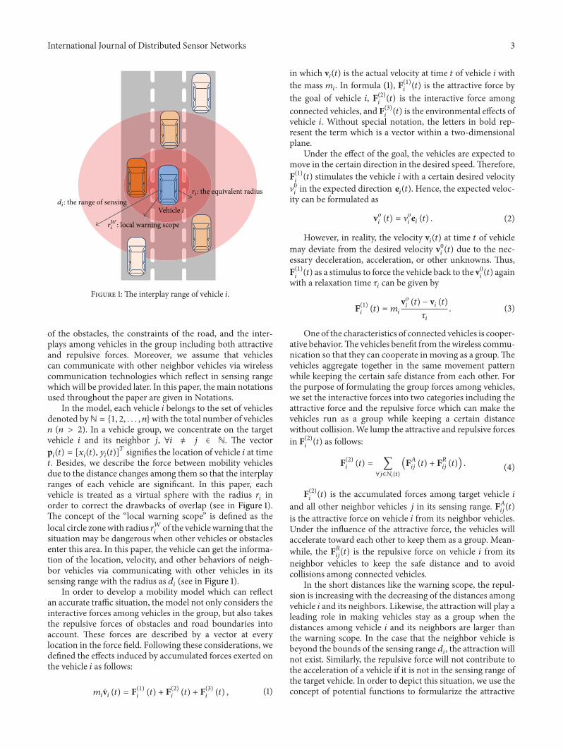
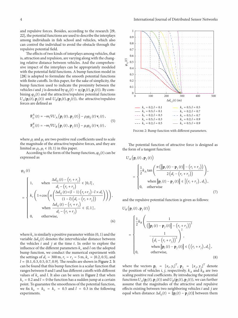
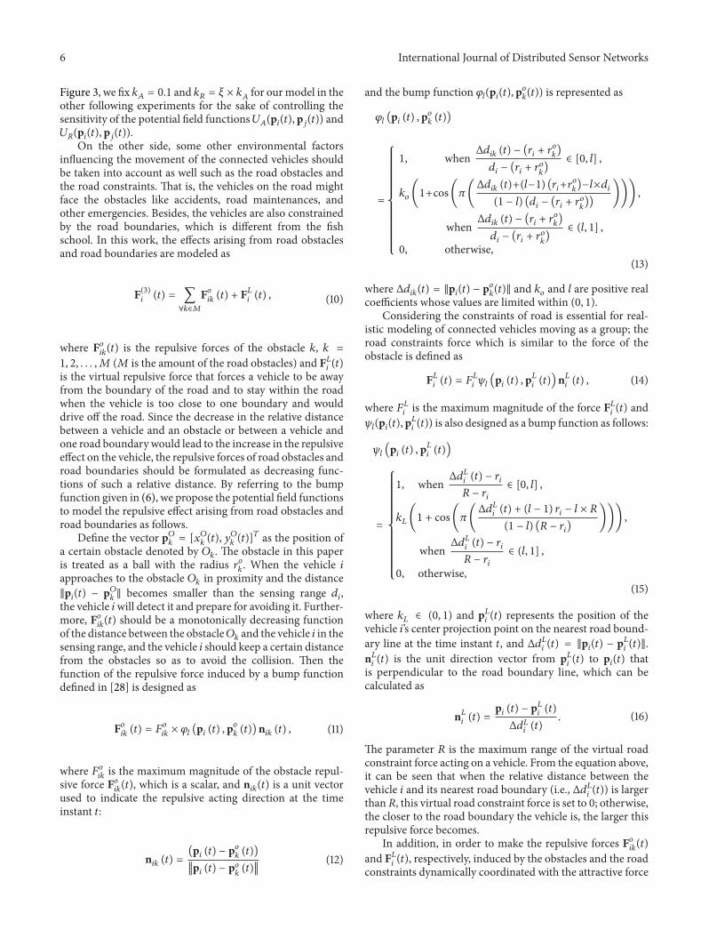
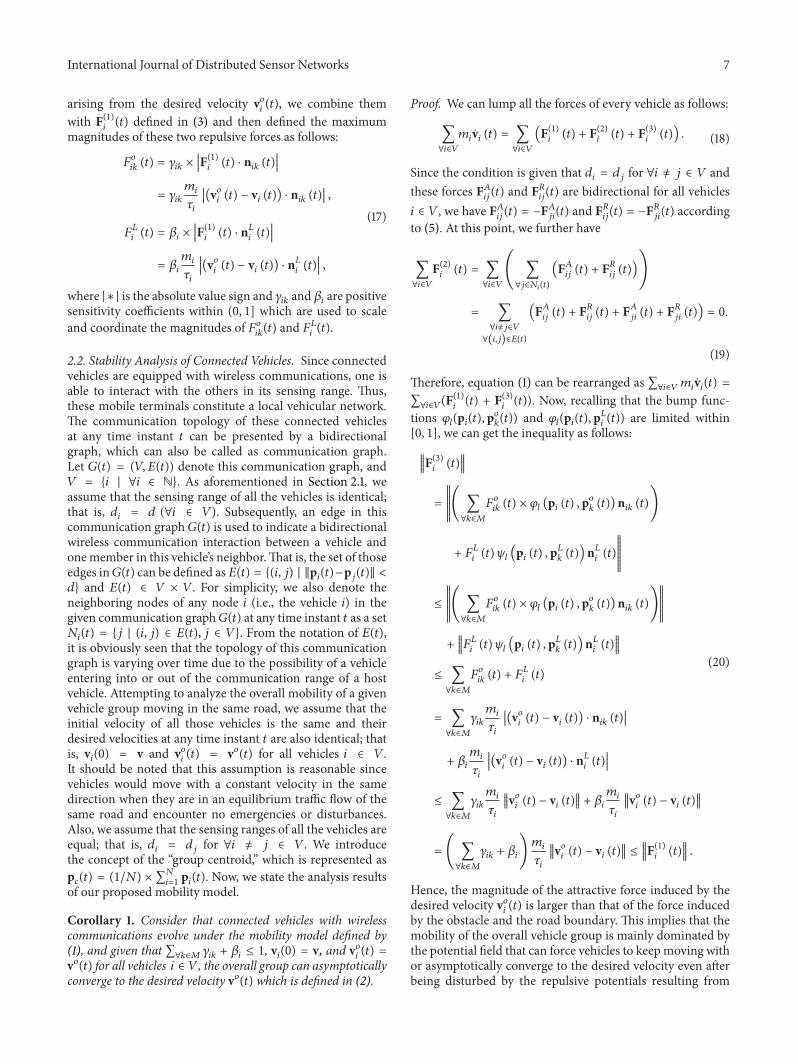
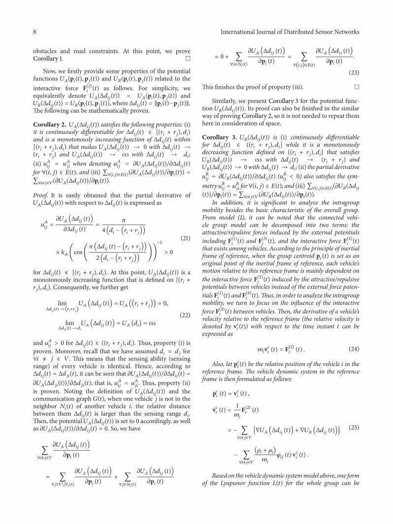
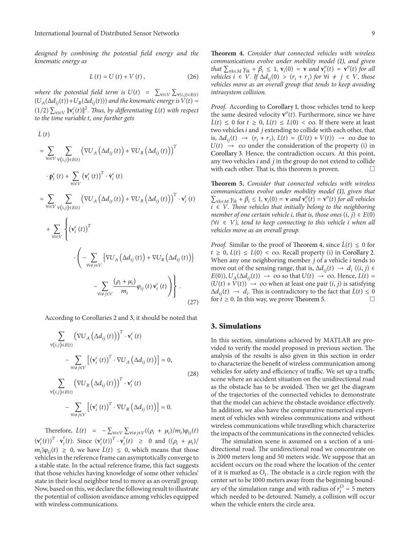
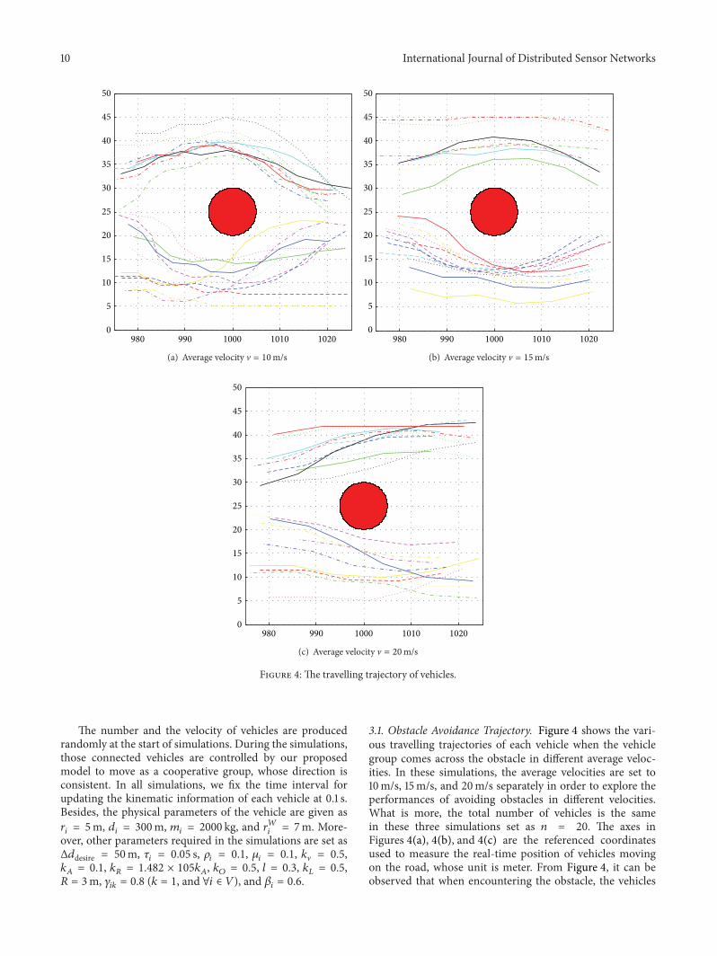
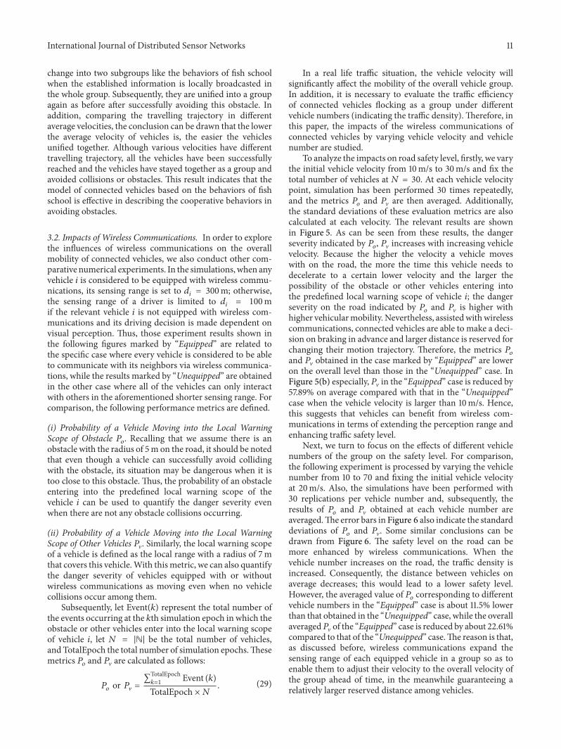
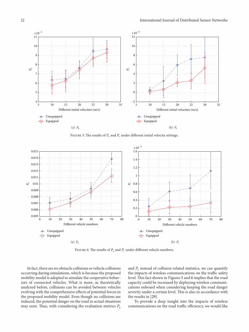
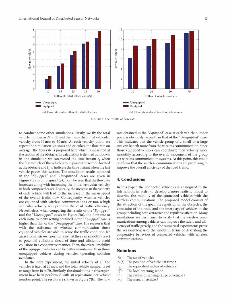

International Journal of
AerospaceEngineeringHindawi Publishing Corporationhttpwwwhindawicom Volume 2014
RoboticsJournal of
Hindawi Publishing Corporationhttpwwwhindawicom Volume 2014
Hindawi Publishing Corporationhttpwwwhindawicom Volume 2014
Active and Passive Electronic Components
Control Scienceand Engineering
Journal of
Hindawi Publishing Corporationhttpwwwhindawicom Volume 2014
International Journal of
RotatingMachinery
Hindawi Publishing Corporationhttpwwwhindawicom Volume 2014
Hindawi Publishing Corporation httpwwwhindawicom
Journal ofEngineeringVolume 2014
Submit your manuscripts athttpwwwhindawicom
VLSI Design
Hindawi Publishing Corporationhttpwwwhindawicom Volume 2014
Hindawi Publishing Corporationhttpwwwhindawicom Volume 2014
Shock and Vibration
Hindawi Publishing Corporationhttpwwwhindawicom Volume 2014
Civil EngineeringAdvances in
Acoustics and VibrationAdvances in
Hindawi Publishing Corporationhttpwwwhindawicom Volume 2014
Hindawi Publishing Corporationhttpwwwhindawicom Volume 2014
Electrical and Computer Engineering
Journal of
Advances inOptoElectronics
Hindawi Publishing Corporation httpwwwhindawicom
Volume 2014
The Scientific World JournalHindawi Publishing Corporation httpwwwhindawicom Volume 2014
SensorsJournal of
Hindawi Publishing Corporationhttpwwwhindawicom Volume 2014
Modelling amp Simulation in EngineeringHindawi Publishing Corporation httpwwwhindawicom Volume 2014
Hindawi Publishing Corporationhttpwwwhindawicom Volume 2014
Chemical EngineeringInternational Journal of Antennas and
Propagation
International Journal of
Hindawi Publishing Corporationhttpwwwhindawicom Volume 2014
Hindawi Publishing Corporationhttpwwwhindawicom Volume 2014
Navigation and Observation
International Journal of
Hindawi Publishing Corporationhttpwwwhindawicom Volume 2014
DistributedSensor Networks
International Journal of