Embed Size (px)
Citation preview
Measurement Valuation of Public Transport Reliability
M Vincent
Booz Allen Hamilton
Land Transport New Zealand Research Report 339
ISBN 978-0-478-30949-2
ISSN 1177-0600 © 2008, Land Transport New Zealand PO Box 2840, 44 Victoria St, Wellington, New Zealand Telephone 64-4 894 5400; Facsimile 64-4 894 6100 Email: [email protected] Website: www.landtransport.govt.nz Vincent, M. 2008 Measurement valuation of public transport reliability. Land Transport New Zealand Research Report 339. 128 pp. Keywords: bus, customer service, delay, evaluation, New Zealand, public expectations, public transport, rail, reliability, surveys, time, valuation
An important note for the reader Land Transport New Zealand is a crown entity established under the Land Transport Management Act 2003. The objective of Land Transport New Zealand is to allocate resources and to undertake its functions in a way that contributes to an integrated, safe, responsive and sustainable land transport system. Each year, Land Transport New Zealand invests a portion of its funds on research that contributes to this objective. The research detailed in this project was commissioned by Land Transport New Zealand. While this report is believed to be correct at the time of its preparation, Land Transport New Zealand, and its employees and agents involved in its preparation and publication, cannot accept any liability for its contents or for any consequences arising from its use. People using the contents of this document, whether directly or indirectly, should apply and rely on their own skill and judgement. They should not rely on its contents in isolation from other sources of advice and information. If necessary, they should seek appropriate legal or other expert advice in relation to their own circumstances, and to the use of this report. The material contained in this report is the output of research and should not be construed in any way as policy adopted by Land Transport New Zealand but may be used in the formulation of future policy.
Acknowledgments The author would like to thank John Bates from Consulting Services, UK, and Pete Clark from Auckland Regional Transport Authority for peer-reviewing this report. Thanks also to the UK Association of Train Operating Companies for their kind permission to publish data from their Passenger Demand Forecasting Handbook.
Abbreviations and acronyms AML: Average Minutes’ Lateness BECA: Beca Carter Hollings & Ferner Ltd. IVT: In-Vehicle Time LUL: London Underground PAT: Preferred Arrival Time RP: Revealed Preference SD: Standard Deviation SP: Stated Preference
5
Contents Executive summary ............................................................................................................. 7 Abstract ............................................................................................................................. 11 1. Introduction ............................................................................................................ 13 1.1 This report ....................................................................................................... 13 1.2 Scope and structure .......................................................................................... 13 2. Overview of reliability.............................................................................................. 14 2.1 Definition of reliability........................................................................................ 14 2.2 Components of public transport reliability............................................................. 15 2.3 Why reliability matters....................................................................................... 16 3. Review of reliability measurement .......................................................................... 18 4. Review of approaches to reliability valuation .......................................................... 22 4.1 Methodologies .................................................................................................. 22 4.2 Options for representing reliability in surveys ....................................................... 23 4.2.1 Existing options ...................................................................................... 23 4.2.2 A set of representative trips ..................................................................... 23 4.2.3 Probability of delay.................................................................................. 28 4.2.4 Predetermined levels of earliness .............................................................. 29 4.3 SP Survey design issues .................................................................................... 29 4.3.1 Basic survey design........................................................................................... 29 4.3.2 Non-traders...................................................................................................... 29 4.3.3 Estimating the range of values............................................................................ 30 5. Review of reliability valuation methods and findings ............................................... 32 5.1 Measures ......................................................................................................... 32 5.2 Approaches for estimating the value of reliability .................................................. 32 5.2.1 Categories.............................................................................................. 32 5.2.2 The mean delay approach ........................................................................ 33 5.2.3 The variance delay approach .................................................................... 33 5.3.4 The scheduling cost approach ................................................................... 34 5.3 Estimating utility functions using Logit models ...................................................... 35 5.4 Valuation findings ............................................................................................. 35 5.4.1 Valuations in the literature ....................................................................... 35 5.4.2 Mean delay valuations ............................................................................. 39 5.4.3 Variance delay valuations......................................................................... 39 5.4.4 Valuation summary ................................................................................. 39 6. Reliability SP survey ................................................................................................ 40 6.1 Possible approaches .......................................................................................... 40 6.2 Why does reliability matter? ............................................................................... 40 6.3 Parameter valuation .......................................................................................... 41 6.4 Presentation of reliability.................................................................................... 42 6.5 SP survey design .............................................................................................. 44 6.6 Survey delivery................................................................................................. 46 6.6.1 Recruitment and delivery ......................................................................... 48 6.6.2 Sample size and selection ........................................................................ 48 6.6.3 Design ................................................................................................... 49 6.6.4 Pilot survey ............................................................................................ 49
6
7. Survey results and implications ............................................................................... 50 7.1 Market segments .............................................................................................. 50 7.2 Passenger trip timing......................................................................................... 51 7.3 Current perceptions and attitudes to reliability...................................................... 52 7.3.1 Method .................................................................................................. 52 7.3.2 Importance of arriving on time ................................................................. 53 7.3.3 Perceptions of current service reliability ..................................................... 54 7.3.4 Attitudes to unreliable services ................................................................. 55 8. Reliability stated preference valuations................................................................... 58 8.1 Model overview................................................................................................. 58 8.1.1 General.................................................................................................. 58 8.1.2 Departure time variability model ............................................................... 59 8.1.3 IVT variability model ............................................................................... 61 8.1.4 Weighting data ....................................................................................... 63 8.1.5 The constant .......................................................................................... 64 8.2 Departure variability model ................................................................................ 65 8.2.1 Summary............................................................................................... 65 8.2.2 Disaggregate model ................................................................................ 67 8.2.3 Mean delay model ................................................................................... 70 8.2.3 Variance model ....................................................................................... 71 8.2.4 Mean-variance model .............................................................................. 73 8.3 In-vehicle variability model ................................................................................ 75 8.3.1 Summary............................................................................................... 75 8.3.2 Disaggregate model ................................................................................ 76 8.3.3 Mean delay model ................................................................................... 79 8.3.4 Variance model ....................................................................................... 80 8.3.5 Mean-variance model .............................................................................. 81 8.4 Comparison of departure and in-vehicle variability models ..................................... 82 8.4.1 Purpose ................................................................................................. 82 8.4.2 Disaggregate model ................................................................................ 82 8.4.3 Mean delay model ................................................................................... 84 8.4.4 Variance model ....................................................................................... 85 8.4.5 Mean-variance model .............................................................................. 86 8.5 Implications for planning – recommended valuations............................................. 87 8.5.1 Summary............................................................................................... 87 8.5.2 Recommended valuations......................................................................... 89 9. Application............................................................................................................... 90 9.1 Journey time in all examples .............................................................................. 90 9.2 Example 1: a service that occasionally runs early.................................................. 90 9.3 Example 2: a service that does not run early........................................................ 91 9.4 Example 3: a small reliability improvement .......................................................... 92 9.5 Application with an Emme/2 modelling process..................................................... 93 10. Further work............................................................................................................ 94 11. References............................................................................................................... 95 Appendices ........................................................................................................................ 99
7
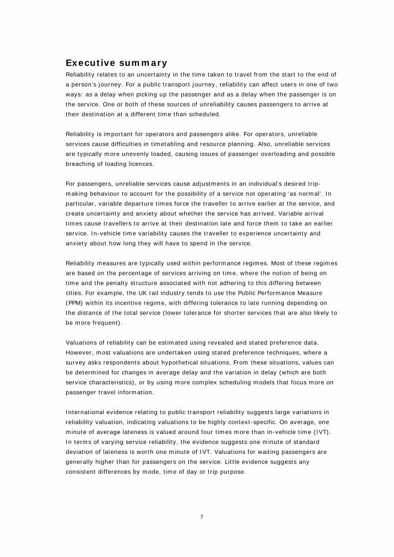
Executive summary Reliability relates to an uncertainty in the time taken to travel from the start to the end of
a person’s journey. For a public transport journey, reliability can affect users in one of two
ways: as a delay when picking up the passenger and as a delay when the passenger is on
the service. One or both of these sources of unreliability causes passengers to arrive at
their destination at a different time than scheduled.
Reliability is important for operators and passengers alike. For operators, unreliable
services cause difficulties in timetabling and resource planning. Also, unreliable services
are typically more unevenly loaded, causing issues of passenger overloading and possible
breaching of loading licences.
For passengers, unreliable services cause adjustments in an individual’s desired trip-
making behaviour to account for the possibility of a service not operating ‘as normal’. In
particular, variable departure times force the traveller to arrive earlier at the service, and
create uncertainty and anxiety about whether the service has arrived. Variable arrival
times cause travellers to arrive at their destination late and force them to take an earlier
service. In-vehicle time variability causes the traveller to experience uncertainty and
anxiety about how long they will have to spend in the service.
Reliability measures are typically used within performance regimes. Most of these regimes
are based on the percentage of services arriving on time, where the notion of being on
time and the penalty structure associated with not adhering to this differing between
cities. For example, the UK rail industry tends to use the Public Performance Measure
(PPM) within its incentive regime, with differing tolerance to late running depending on
the distance of the total service (lower tolerance for shorter services that are also likely to
be more frequent).
Valuations of reliability can be estimated using revealed and stated preference data.
However, most valuations are undertaken using stated preference techniques, where a
survey asks respondents about hypothetical situations. From these situations, values can
be determined for changes in average delay and the variation in delay (which are both
service characteristics), or by using more complex scheduling models that focus more on
passenger travel information.
International evidence relating to public transport reliability suggests large variations in
reliability valuation, indicating valuations to be highly context-specific. On average, one
minute of average lateness is valued around four times more than in-vehicle time (IVT).
In terms of varying service reliability, the evidence suggests one minute of standard
deviation of lateness is worth one minute of IVT. Valuations for waiting passengers are
generally higher than for passengers on the service. Little evidence suggests any
consistent differences by mode, time of day or trip purpose.
MEASUREMENT VALUATION OF PUBLIC TRANSPORT RELIABILITY
8
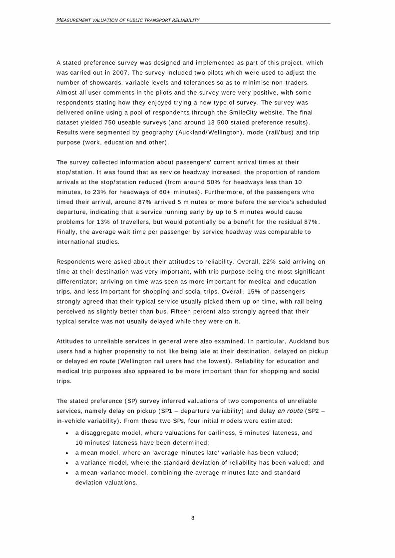
A stated preference survey was designed and implemented as part of this project, which
was carried out in 2007. The survey included two pilots which were used to adjust the
number of showcards, variable levels and tolerances so as to minimise non-traders.
Almost all user comments in the pilots and the survey were very positive, with some
respondents stating how they enjoyed trying a new type of survey. The survey was
delivered online using a pool of respondents through the SmileCity website. The final
dataset yielded 750 useable surveys (and around 13 500 stated preference results).
Results were segmented by geography (Auckland/Wellington), mode (rail/bus) and trip
purpose (work, education and other).
The survey collected information about passengers’ current arrival times at their
stop/station. It was found that as service headway increased, the proportion of random
arrivals at the stop/station reduced (from around 50% for headways less than 10
minutes, to 23% for headways of 60+ minutes). Furthermore, of the passengers who
timed their arrival, around 87% arrived 5 minutes or more before the service’s scheduled
departure, indicating that a service running early by up to 5 minutes would cause
problems for 13% of travellers, but would potentially be a benefit for the residual 87%.
Finally, the average wait time per passenger by service headway was comparable to
international studies.
Respondents were asked about their attitudes to reliability. Overall, 22% said arriving on
time at their destination was very important, with trip purpose being the most significant
differentiator; arriving on time was seen as more important for medical and education
trips, and less important for shopping and social trips. Overall, 15% of passengers
strongly agreed that their typical service usually picked them up on time, with rail being
perceived as slightly better than bus. Fifteen percent also strongly agreed that their
typical service was not usually delayed while they were on it.
Attitudes to unreliable services in general were also examined. In particular, Auckland bus
users had a higher propensity to not like being late at their destination, delayed on pickup
or delayed en route (Wellington rail users had the lowest). Reliability for education and
medical trip purposes also appeared to be more important than for shopping and social
trips.
The stated preference (SP) survey inferred valuations of two components of unreliable
services, namely delay on pickup (SP1 – departure variability) and delay en route (SP2 –
in-vehicle variability). From these two SPs, four initial models were estimated:
• a disaggregate model, where valuations for earliness, 5 minutes’ lateness, and
10 minutes’ lateness have been determined;
• a mean model, where an ‘average minutes late’ variable has been valued;
• a variance model, where the standard deviation of reliability has been valued; and
• a mean-variance model, combining the average minutes late and standard
deviation valuations.
9
The disaggregate model indicated that valuations of earliness, being late by 5 minutes,
and being late by 10 minutes were different on an equivalent per minute basis. For
services that ran early, valuations on departure were highest (because of the possibility of
missing the service), whilst valuations on the vehicle were lowest (because of the benefits
of reduced travel times for some passengers). Valuations of 10 minutes’ lateness were
higher than 5 minutes’ lateness, indicating that passengers become more agitated as
delays increase. It should be noted, however, that the high valuation of early time on
departure was some-what at odds with the proportion of passengers who might be
affected by an early service. This finding requires more investigation.
A mean delay model was then estimated, using average minutes’ lateness as a measure.
This is the approach that is most widely adopted internationally to apply reliability
impacts. Overall, it was found respondents place a higher value on average unexpected
wait time (delay at departure) than average delay en route, with rail valuations lower
than bus. Valuations were similar to those found in other international studies and
recommended parameters in demand forecasting handbooks.
The variance delay model determined valuations of the standard deviation of wait and in-
vehicle times. Interestingly, respondents placed a higher value on in-vehicle variability
than departure variability, which was opposite to the average delay behaviour. Valuations
were high by international valuations, although a large spread in these valuations makes
comparison difficult.
A combined mean-variance delay model was fitted. However, this was found to generate
negative valuations for standard deviation in some segments. Therefore, this formulation
was not taken further.
From the departure SP, a value of time could be determined. The range in values of time
(VoT) were around $8/hr, which is higher than the numbers currently used in the
Economic Evaluation Manual (EEM) ($4.70/hr for commuting, $3.05 for other); however,
these are 2002 prices and probably include a younger market. Also, the EEM assumes the
same VoT for rail and bus users, but the SP survey found rail users consistently had a
value of time almost twice that of bus users. Higher VoTs for rail users are generally
found internationally.
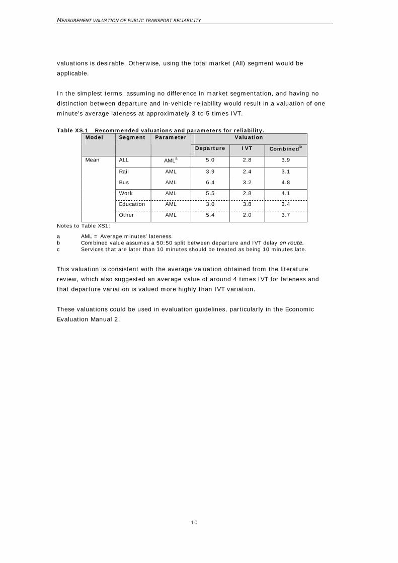
The preferred approach, based on ease of use and comparability to international
measures, was to use the mean delay model with average minutes’ lateness and the
valuations given in Table XS.1. Valuations are provided for delay on departure and delay
in-vehicle. Wherever possible, the different sources of delay should be applied to each
proportion of demand affected by such delay. This could be undertaken by looking at the
major sources of time variation through a route’s itinerary, and determining the
proportion of users on the service and to be picked up by the service at each point.
Valuations are also split by mode (rail and bus) and purpose (work, education and other).
If demand data are available from any of these segments then using the segment-based
MEASUREMENT VALUATION OF PUBLIC TRANSPORT RELIABILITY
10
valuations is desirable. Otherwise, using the total market (All) segment would be
applicable.
In the simplest terms, assuming no difference in market segmentation, and having no
distinction between departure and in-vehicle reliability would result in a valuation of one
minute’s average lateness at approximately 3 to 5 times IVT.
Table XS.1 Recommended valuations and parameters for reliability.
Valuation Model Segment Parameter
Departure IVT Combinedb
ALL AMLa 5.0 2.8 3.9
Rail AML 3.9 2.4 3.1
Bus AML 6.4 3.2 4.8
Work AML 5.5 2.8 4.1
Education AML 3.0 3.8 3.4
Mean
Other AML 5.4 2.0 3.7
Notes to Table XS1:
a AML = Average minutes’ lateness. b Combined value assumes a 50:50 split between departure and IVT delay en route. c Services that are later than 10 minutes should be treated as being 10 minutes late.
This valuation is consistent with the average valuation obtained from the literature
review, which also suggested an average value of around 4 times IVT for lateness and
that departure variation is valued more highly than IVT variation.
These valuations could be used in evaluation guidelines, particularly in the Economic
Evaluation Manual 2.
11
Abstract
Reliability in public transport is important for operators and passengers alike. Reliability
can affect users in one of two ways: as a delay when picking up the passenger and as a
delay when the passenger is on the service. Reliability measures are typically used within
performance regimes to evaluate the quality of service of public transport providers.
This research, carried out in 2007, aims to find a method of measuring the value placed
on public transport reliability in different contexts in New Zealand. As part of this project,
a stated preference survey was designed and implemented to collect information about
passengers’ current public transport usage, their attitudes to reliability and how they
valued reliability.
Using these stated preference surveys, four initial models were estimated: a disaggregate
model, a mean model, a variance model and a mean-variance model. The preferred
approach, based on ease of use and comparability to international measures, was the
mean delay model.
A value of time was determined from the departure stated preference survey. Values of
time ranged around $8/hour. The surveys also found that rail users consistently had a
value of time almost twice that of bus users, which is consistent with international
findings.

MEASUREMENT VALUATION OF PUBLIC TRANSPORT RELIABILITY
12
1. Introduction
13
1 Introduction
1.1 This report
This report has been developed by Booz Allen Hamilton as part of the Land Transport
New Zealand Research Programme 2005–2006, primarily to examine the valuation of
public transport reliability and implications within the New Zealand planning context. The
research was carried out in 2007.
The process has involved the development of this report, a survey conducted in
conjunction with a market research company, and a peer review which examined the
report and processes.
1.2 Scope and structure
The report provides an overview of the concept of reliability, particularly the impact that
service reliability has on passengers and operators. Reliability measurement methods and
monitoring processes are explored. An international review of reliability valuation
methods is undertaken. Based on this review, a reliability valuation approach is applied to
a New Zealand context. Finally, the implications of the approach for planning are outlined.
The report is structured as follows:
• Chapter 2: Overview of reliability,
• Chapter 3: Review of reliability measurement methods,
• Chapter 4: Review of approaches to reliability valuation,
• Chapter 5: Review of reliability valuation methods and findings,
• Chapter 6: Reliability state preference survey,
• Chapter 7: Survey results and implications,
• Chapter 8: Reliability stated preference valuations.
MEASUREMENT VALUATION OF PUBLIC TRANSPORT RELIABILITY
14
2 Overview of reliability
2.1 Definition of reliability
The term ‘reliability’ within a transport context relates to an uncertainty in the time taken
to travel from the start to the end of a person’s journey. This uncertainty means that a
person must make some allowance in the timing of their journey to allow for this
uncertainty so that they can still reach the end within a desirable time band. Within
transport, different modes have different sources of reliability which relate to uncertainty
within individual aspects of their journey.
In transport economics, generalised cost is used to represent the total user cost for a
journey; this provides a useful framework to categorise reliability aspects. User costs
when travelling by car are primarily comprised of the time taken, the operating cost of
the vehicle and a parking cost. Variations of travel time occur particularly on heavily
congested roads, where the deviations of other individuals’ departure times or a one-off
event (such as an accident or breakdown) can cause significant changes in delays.
Variations in operating cost are less apparent to users, but could include unexpected
maintenance on their vehicle. Variations in parking costs are usually ignored, but could
involve extra time taken to find a park or an additional cost for having to park in a more
expensive area than usual.
Public transport has similar sources of uncertainty, but the main difference from using a
car is the reduced level of control users have over their own situation caused primarily by
the reduced flexibility of public transport; car users can time their journey ‘to the minute’
whereas a public transport user needs to keep to an existing timetable. For a public
transport user, the journey consists mainly of:
• travel time spent in the vehicle and access/egress to the vehicle), known as in-
vehicle time (IVT);
• the time taken waiting for the service; and
• the fare paid.
In-vehicle travel time variations are usually caused by either infrastructure or vehicle
failure. Waiting time variation is caused primarily by a previous in-vehicle time variation,
but can also be caused by service cancellation. Waiting time variation is seen by a user as
a delay to their departure from the stop/station.
For a public transport user, if a service is running early, he/she faces the real possibility
that they may miss it given their arrival time at the stop/station. In this situation, a user
would then have to wait for the next service, thus increasing their wait time substantially.
2. Overview of reliability
15
2.2 Components of public transport reliability
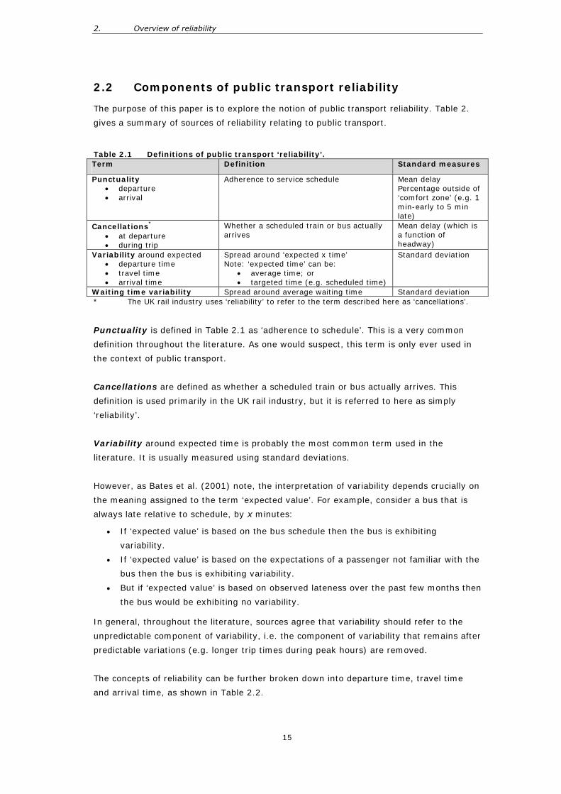
The purpose of this paper is to explore the notion of public transport reliability. Table 2.
gives a summary of sources of reliability relating to public transport.
Table 2.1 Definitions of public transport ‘reliability’. Term Definition Standard measures
Punctuality • departure • arrival
Adherence to service schedule Mean delay Percentage outside of ‘comfort zone’ (e.g. 1 min-early to 5 min late)
Cancellations* • at departure • during trip
Whether a scheduled train or bus actually arrives
Mean delay (which is a function of headway)
Variability around expected • departure time • travel time • arrival time
Spread around ‘expected x time’ Note: ‘expected time’ can be:
• average time; or • targeted time (e.g. scheduled time)
Standard deviation
Waiting time variability Spread around average waiting time Standard deviation * The UK rail industry uses ‘reliability’ to refer to the term described here as ‘cancellations’.
Punctuality is defined in Table 2.1 as ‘adherence to schedule’. This is a very common
definition throughout the literature. As one would suspect, this term is only ever used in
the context of public transport.
Cancellations are defined as whether a scheduled train or bus actually arrives. This
definition is used primarily in the UK rail industry, but it is referred to here as simply
‘reliability’.
Variability around expected time is probably the most common term used in the
literature. It is usually measured using standard deviations.
However, as Bates et al. (2001) note, the interpretation of variability depends crucially on
the meaning assigned to the term ‘expected value’. For example, consider a bus that is
always late relative to schedule, by x minutes:
• If ‘expected value’ is based on the bus schedule then the bus is exhibiting
variability.
• If ‘expected value’ is based on the expectations of a passenger not familiar with the
bus then the bus is exhibiting variability.
• But if ‘expected value’ is based on observed lateness over the past few months then
the bus would be exhibiting no variability.
In general, throughout the literature, sources agree that variability should refer to the
unpredictable component of variability, i.e. the component of variability that remains after
predictable variations (e.g. longer trip times during peak hours) are removed.
The concepts of reliability can be further broken down into departure time, travel time
and arrival time, as shown in Table 2.2.
MEASUREMENT VALUATION OF PUBLIC TRANSPORT RELIABILITY
16
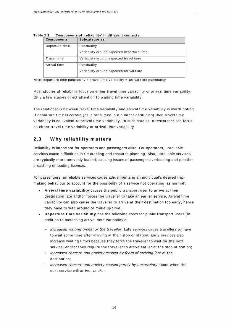
Table 2.2 Components of ‘reliability’ in different contexts. Components Subcategories
Departure time Punctuality
Variability around expected departure time
Travel time Variability around expected travel time
Arrival time Punctuality
Variability around expected arrival time
Note: departure time punctuality + travel time variability = arrival time punctuality
Most studies of reliability focus on either travel time variability or arrival time variability.
Only a few studies direct attention to waiting time variability.
The relationship between travel time variability and arrival time variability is worth noting.
If departure time is certain (as is presumed in a number of studies) then travel time
variability is equivalent to arrival time variability. In such studies, a researcher can focus
on either travel time variability or arrival time variability
2.3 Why reliability matters
Reliability is important for operators and passengers alike. For operators, unreliable
services cause difficulties in timetabling and resource planning. Also, unreliable services
are typically more unevenly loaded, causing issues of passenger overloading and possible
breaching of loading licences.
For passengers, unreliable services cause adjustments in an individual’s desired trip-
making behaviour to account for the possibility of a service not operating ‘as normal’.
• Arrival time variability causes the public transport user to arrive at their
destination late and/or forces the traveller to take an earlier service. Arrival time
variability can also cause the traveller to arrive at their destination too early, hence
they have to wait around or make up time.
• Departure time variability has the following costs for public transport users (in
addition to increasing arrival time variability):
– increased waiting times for the traveller. Late services cause travellers to have
to wait some time after arriving at their stop or station. Early services also
increase waiting times because they force the traveller to wait for the next
service, and/or they require the traveller to arrive earlier at the stop or station;
– increased concern and anxiety caused by fears of arriving late at the
destination;
– increased concern and anxiety caused purely by uncertainty about when the
next service will arrive; and/or
2. Overview of reliability
17
– increased likelihood of a late service that, because of its lateness, picks up more
people and hence forces additional passengers to ride standing and/or in
crowded conditions1.
• In-vehicle-time (IVT) variability has the following costs for public transport
users (in addition to increasing arrival time variability):
– increased concern and anxiety caused by fears of arriving late at the destination,
– increased concern and anxiety caused by uncertainty about how long they will
have to spend in the service, and
– increased variability surrounding how long the passenger will have to spend
standing and/or in crowded conditions.
The research focuses on passenger attitudes to service reliability and will investigate how
the population of interest values the different components (listed above) of public
transport reliability.
1 The increased likelihood of standing or crowdedness may not be significant but is noted here because it may be included in valuations.
MEASUREMENT VALUATION OF PUBLIC TRANSPORT RELIABILITY
18
3 Review of reliability measurement methods
Reliability measurement methods are used throughout the world as a way for authorities
to penalise passenger transport operators for poor performance. In general, the
measurements used have a lot in common, the major differences being the tolerances
that are applied and the subsequent penalty regimes.
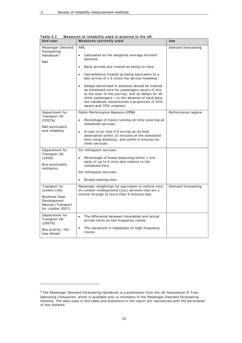
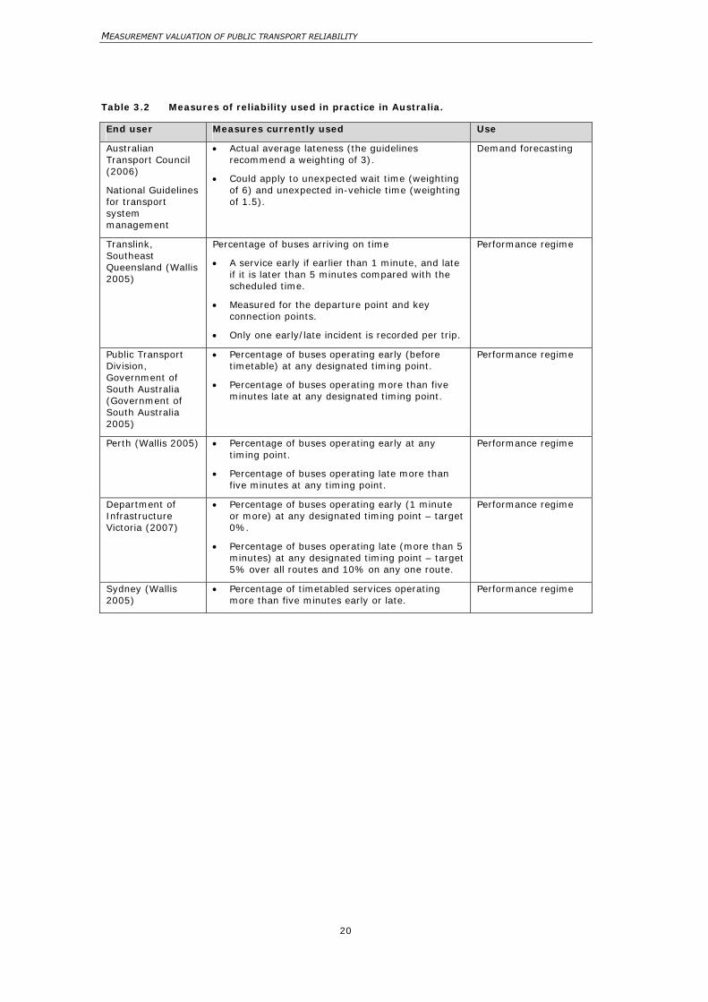
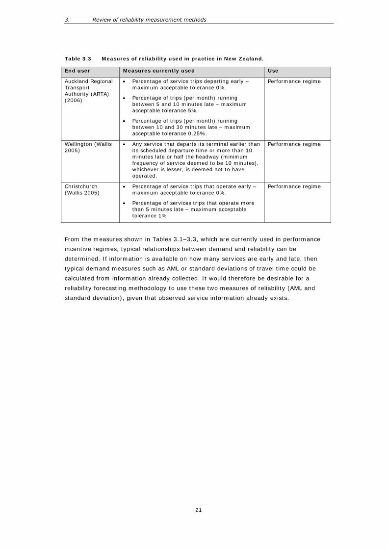
Tables 3.1–3.3 provide a summary of some reliability measures that are used in practice
by authorities and planners. Measures are typically used for two purposes:
• to aid in forecasting demand changes as a result of performance changes, and
• as a measure included in penalising/rewarding operators for bad/good performance.
In terms of demand forecasting, the UK rail industry typically uses Average Minutes’
Lateness (AML) as a measure of reliability. Much of the literature on how passengers
respond to changes in reliability is based around changes in the average delay that
passengers experience, and this has been used as a recommended forecasting approach
with appropriate weightings and levels of flexibility. For the London Underground, demand
responses for forecasting are usually undertaken on a more disaggregate level where
detailed information about individual services is available and service frequencies are
high. As such, the London Underground adopts an individual passenger response for a
given service depending on how long it is delayed.
Reliability measures are typically used within performance regimes. Most of these regimes
are based on the percentage of services arriving on time, where the notion of being on
time and the penalty structure associated with not adhering to this differing between
cities. For example, the UK rail industry tends to use the Public Performance Measure
(PPM) within its incentive regime, with differing tolerance to late running depending on
the distance of the total service (lower tolerance for shorter services).
For bus services, tolerances are much lower, with a typical tolerance of late running of 5
minutes from timetable schedule. However, some cities distinguish between late running
(typically 5 minutes) and extremely late running (later than 10 minutes). Services
running early are not commonly tolerated, with many cities expecting services to run at
least on time at timing points – although examples that allow for one minute’s earliness
exist.
3. Review of reliability measurement methods
19
Table 3.1 Measures of reliability used in practice in the UK. End user Measures currently used Use
Passenger Demand Forecasting Handbook2
Rail
AML
• Calculated as the weighted average minutes’ lateness.
• Early arrivals are treated as being on time.
• Cancellations treated as being equivalent to a late arrival of 1.5 times the service headway.
• Delays advertised in advance should be treated as scheduled time for passengers aware of this at the start of the journey, and as delays for all other passengers – in the absence of hard data, the handbook recommends a proportion of 25% aware and 75% unaware.
Demand forecasting
Department for Transport UK (2007a)
Rail punctuality and reliability
Public Performance Measure (PPM)
• Percentage of trains running on time covering all scheduled services.
• A train is on time if it arrives at its final destination within 10 minutes of the scheduled time (long distance), and within 5 minutes for other services.
Performance regime
Department for Transport UK (2006)
Bus punctuality indicators
For infrequent services:
• Percentage of buses departing within 1 min early or up to 5 mins late relative to the scheduled time.
For infrequent services:
• Excess waiting time.
Transport for London (UK)
Business Case Development Manual (Transport for London 2007)
Passenger weightings for equivalent in-vehicle time on London Underground (LUL) services that are 1 minute through to more than 9 minutes late,
Demand forecasting
Department for Transport UK (2007b)
Bus priority: the way ahead
• The difference between timetabled and actual arrival times on low-frequency routes.
• The variations in headways on high-frequency routes.
2 The Passenger Demand Forecasting Handbook is a publication from the UK Association of Train Operating Companies, which is available only to members of the Passenger Demand Forecasting Scheme. The data used in this table and elsewhere in the report are reproduced with the permission of this Scheme.
MEASUREMENT VALUATION OF PUBLIC TRANSPORT RELIABILITY
20
Table 3.2 Measures of reliability used in practice in Australia.
End user Measures currently used Use
Australian Transport Council (2006)
National Guidelines for transport system management
• Actual average lateness (the guidelines recommend a weighting of 3).
• Could apply to unexpected wait time (weighting of 6) and unexpected in-vehicle time (weighting of 1.5).
Demand forecasting
Translink, Southeast Queensland (Wallis 2005)
Percentage of buses arriving on time
• A service early if earlier than 1 minute, and late if it is later than 5 minutes compared with the scheduled time.
• Measured for the departure point and key connection points.
• Only one early/late incident is recorded per trip.
Performance regime
Public Transport Division, Government of South Australia (Government of South Australia 2005)
• Percentage of buses operating early (before timetable) at any designated timing point.
• Percentage of buses operating more than five minutes late at any designated timing point.
Performance regime
Perth (Wallis 2005) • Percentage of buses operating early at any timing point.
• Percentage of buses operating late more than five minutes at any timing point.
Performance regime
Department of Infrastructure Victoria (2007)
• Percentage of buses operating early (1 minute or more) at any designated timing point – target 0%.
• Percentage of buses operating late (more than 5 minutes) at any designated timing point – target 5% over all routes and 10% on any one route.
Performance regime
Sydney (Wallis 2005)
• Percentage of timetabled services operating more than five minutes early or late.
Performance regime
3. Review of reliability measurement methods
21
Table 3.3 Measures of reliability used in practice in New Zealand.
From the measures shown in Tables 3.1–3.3, which are currently used in performance
incentive regimes, typical relationships between demand and reliability can be
determined. If information is available on how many services are early and late, then
typical demand measures such as AML or standard deviations of travel time could be
calculated from information already collected. It would therefore be desirable for a
reliability forecasting methodology to use these two measures of reliability (AML and
standard deviation), given that observed service information already exists.
End user Measures currently used Use
Auckland Regional Transport Authority (ARTA) (2006)
• Percentage of service trips departing early – maximum acceptable tolerance 0%.
• Percentage of trips (per month) running between 5 and 10 minutes late – maximum acceptable tolerance 5%.
• Percentage of trips (per month) running between 10 and 30 minutes late – maximum acceptable tolerance 0.25%.
Performance regime
Wellington (Wallis 2005)
• Any service that departs its terminal earlier than its scheduled departure time or more than 10 minutes late or half the headway (minimum frequency of service deemed to be 10 minutes), whichever is lesser, is deemed not to have operated.
Performance regime
Christchurch (Wallis 2005)
• Percentage of service trips that operate early – maximum acceptable tolerance 0%.
• Percentage of services trips that operate more than 5 minutes late – maximum acceptable tolerance 1%.
Performance regime
MEASUREMENT VALUATION OF PUBLIC TRANSPORT RELIABILITY
22
4 Review of approaches to reliability valuation
4.1 Methodologies
Two main methodologies are used to determine people’s valuations of transport costs:
revealed preference (RP) and stated preference (SP) analysis. RP analysis examines the
before and after situation of a given change in transport supply and can be used to
determine people’s response to this change. In other words, RP determines people’s
responses to changes in transport based on what they actually did. Whilst RP analysis is
usually the preferred approach, it is rarely undertaken (particularly in a transport context)
because:
• it is difficult to get consistent before and after data, therefore making it hard to
undertake a comparison;
• many factors affect people’s transport behaviour and it is unlikely that these factors
will remain constant over the period of interest (for example, an improvement in
reliability may be linked to the introduction of new rolling stock, with increased
passenger numbers including the response to the new rolling stock as well as the
reliability improvements. Separating these effects and interpreting the results is
challenging);
• RP analysis requires situations where change has occurred and, once a situation is
found, it may not be applicable to the transport market of interest – it cannot be
used to examine hypothetical situations;
• RP analysis is generally based on patronage numbers with no ability to question
individuals fully and therefore to understand the drivers and market segmentation
of particular responses;
• RP data can include measurement error (or mis-specification) of the dependent
variable. In a reliability example, RP data may use AML as a measure of reliability
but for passengers, it might be the variation in reliability that is more important.
Similarly, where the use of average lateness is appropriate, it may not be measured
correctly or to a sufficient level of detail to discern passenger responses.
Most of the literature therefore focuses on SP approaches to reliability valuation. SP
analysis differs significantly from RP analysis in that it asks respondents how they would
behave given a series of alternatives (scenarios). Respondents are presented with a
number of alternatives (usually two) that differ in the values of their transport costs, and
are asked to choose which alternative they prefer. By varying the costs in an appropriate
way, the alternative a respondent chooses can be used to determine valuations for the
individual transport costs.
SP analysis overcomes all of the difficulties of RP analysis as listed above but has
shortcomings of its own. In particular, some respondents do not actually behave as they
do hypothetically. Some respondents may have their own agenda, and therefore either
give unrealistic answers or the answers they think the survey is looking for. Respondents
4. Review of approaches to reliability valuation
23
may not fully appreciate the impact of the hypothetical examples presented. For example,
presenting a scenario where their fare is doubled may not invoke the same reaction as
their fare actually being doubled and more money leaving their pocket. SP surveys usually
ask respondents about a number of differing scenarios; therefore, surveys can become
tiresome and fatigue biases can be an issue. Surveys need to be fairly simplistic,
particularly when asking a respondent to decide between two options.
Given that most of the reliability literature focuses on SP analysis, and that an SP survey
has been conducted as part of this project, the review of analysis methods focuses on SP
rather than RP. In particular, it will discuss the representation and functional form of SP
reliability studies.
4.2 Options for representing reliability in SP surveys
4.2.1 Existing options
The literature shows that reliability is generally represented in these forms:
• as a set of representative trips (maybe in a week or fortnight),
• as a maximum travel time delay,
• as a probability of delay, or
• as predetermined levels of earliness/lateness.
These are discussed in turn.
4.2.2 A set of representative trips
Many reliability studies associate each alternative presented to a respondent with a set of
representative trips. The representative trips convey a sense of the distribution associated
with that option, and can be used to present either a distribution of travel times or a
distribution of departure/arrival times. As noted earlier, the two representations are
mathematically related if departure time occurs at a definite, pre-determined time.
A set of representative travel times has the advantage that it is ‘realistic’ – it accords
well with reality – and it conveys a lot of information about a distribution in an intuitive
manner. However, for public transport users, departure and arrival times are also
important, as passengers need to adhere to the schedule.
A set of representative departure/arrival times can be easier to comprehend,
especially if represented in terms of minutes earlier or later. However, these surveys
carry a risk of misinterpretation, as will be discussed later.
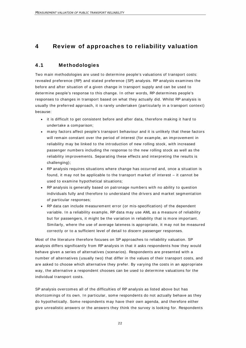
These trips are represented either by numbers or graphs (the most common approach is
to represent travel times as numbers). The layout below (Figure 4.1) is a quintessential
example of the sort of SP surveys used in Small et al. (1995), based on work undertaken
by Black & Towriss (1993).
MEASUREMENT VALUATION OF PUBLIC TRANSPORT RELIABILITY
24
Figure 4.1 SP survey layout as used by Small et al. (1995).
Black & Towriss also introduced a few notable variations to make the options clearer:
• A box was placed around the approximate mean of the distribution of times:
e.g. 38 50 60 74 90
• A message was placed between the two sets of journey times:
e.g. ‘SAME AVERAGE TIME’
• A box was added (under the more variable option) to emphasise that it is the more
variable option:
e.g. TRAVEL TIMES MORE VARIABLE
A pilot survey by Black & Towriss (1993) indicated that arrivals are best represented as
‘minutes earlier or later than planned’. The researchers presented respondents with
reliability in the following forms:
• a tabular form – the number of arrivals falling into given categories of earliness and
lateness,
• a textual list – the representation of arrivals in the form of minutes earlier or later
than planned,
• a set of cards with exact arrival times, and
• a set of clocks – the clocks depicted arrival times and stated the likelihood of
arriving at a particular time.
The rankings produced by the pilot survey were compared with the standard deviations to
see which representation of reliability was most effective at producing the ‘correct’
rankings. The researchers found that the ‘minutes early or late’ representation was
preferred, especially by respondents with little or no numerical background. Black &
Towriss (1993) identified a problem with the ‘minutes early or late’ representation:
respondents in the pilot survey who imagined their trip as not having a timing constraint
were unable to comprehend the exercise. This prompted Black & Towriss to switch to
journey times for the final survey.
Time: minutes
12 13 14 16 20
Time: minutes
5 7 9 1 2 1 8
Departure 15 minutes before your usual arrival time.
Departure 10 minutes before your usual arrival time.
Sample stated preference question
4. Review of approaches to reliability valuation
25
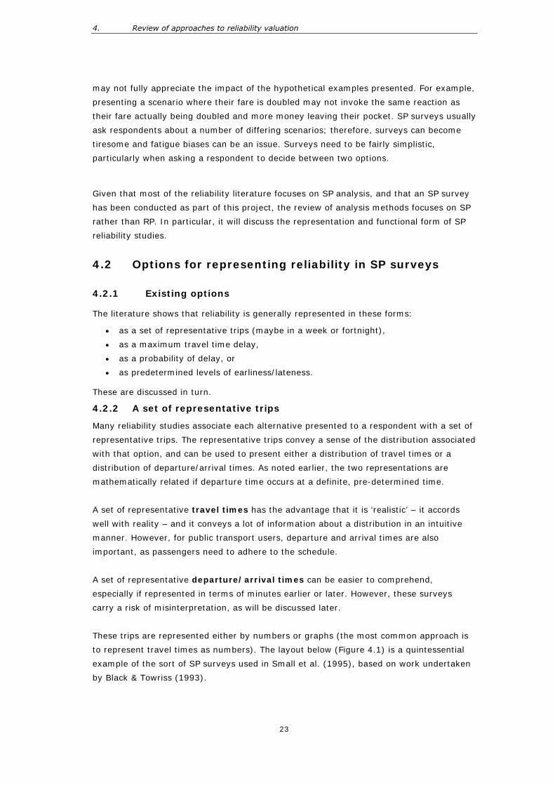
The order in which the trips are represented might become problematic; Bates et al.
(2001) posit that the order of a ‘Benwell & Black’ (1984) series of delays (e.g. 0, 0, 0, 0,
0, 5, 10, 25) may be misinterpreted. For example, people might assume a deteriorating
service level. Or infrequent travellers might assume that they would not incur the delays.
Therefore, Bates et al. (2001) proposed and implemented the ‘clockface’ design (shown in
Figure 4.2), in which ‘order’ is removed.
Figure 4.2 SP survey design used by Bates et al. (2001).
Cook et al (1999) referred to the Black & Towriss (1993) pilot survey discussed above and
chose to use the ‘minutes early or late’ representation in their study of rail commuters.
However, Cook et al. encountered a problem with that representation: respondents
appeared to gravitate towards zeroes. The researchers presented respondents with the
following options:
• A: 1E 1E 1E 1L 1L 1L 5L 10L 10L 35L
• B: 1E 0 0 0 0 1L 5L 25L 25L 35L
Twenty-six percent of respondents preferred Option B, despite 90% saying that they
would not consider a delay of one minute as being late at all.
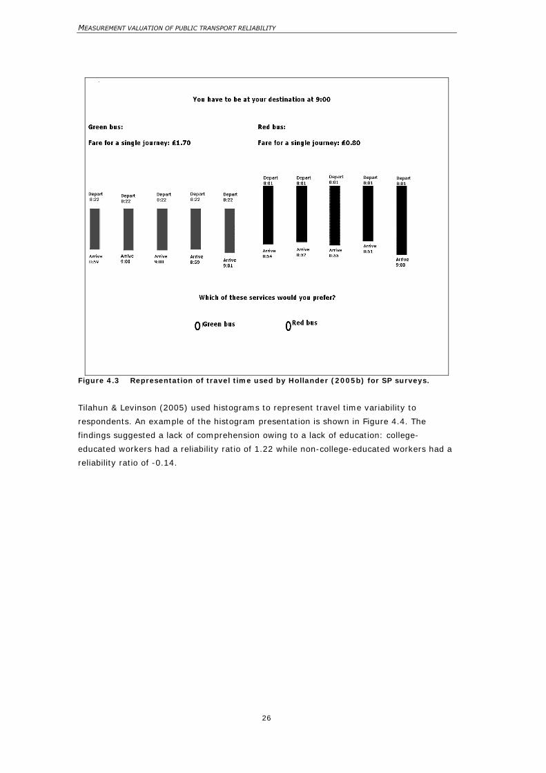
Hollander (2005b) introduced a novel method of representing travel time for his SP
survey of car, bus and rail commuters: departure and arrival times were represented by
the relative locations of the bar, with the bar length giving journey time (as shown in
Figure 4.3).
MEASUREMENT VALUATION OF PUBLIC TRANSPORT RELIABILITY
26
Figure 4.3 Representation of travel time used by Hollander (2005b) for SP surveys.
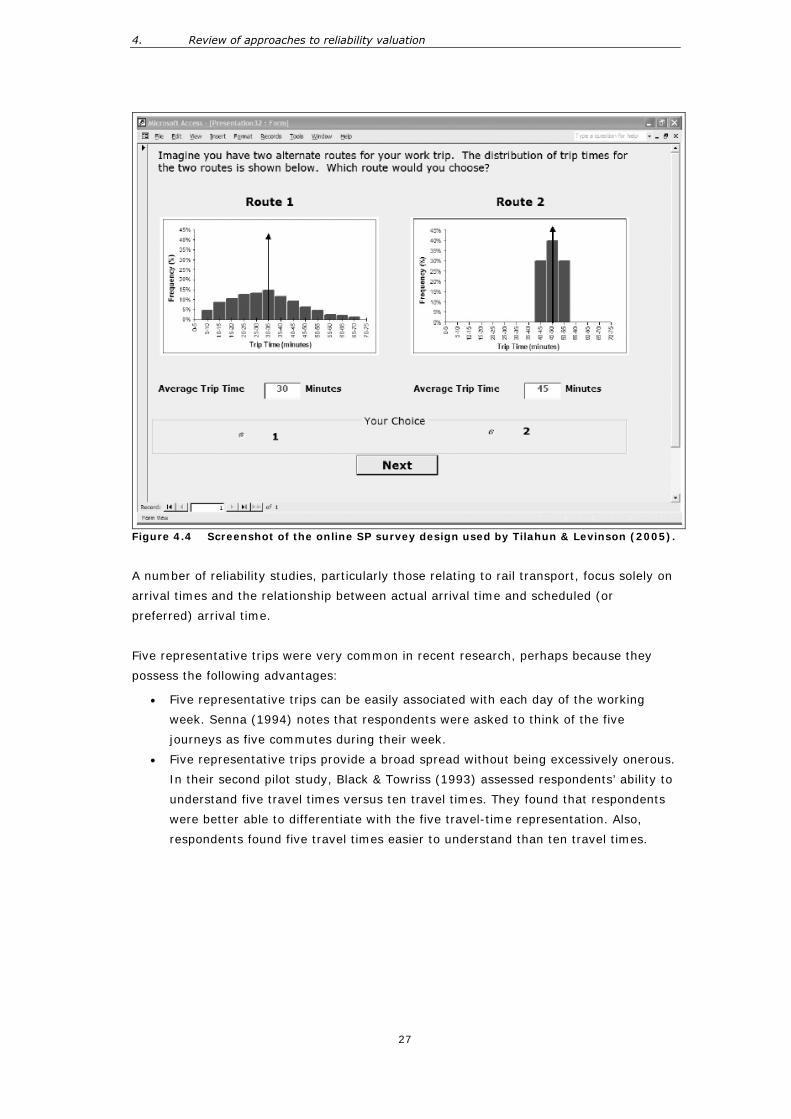
Tilahun & Levinson (2005) used histograms to represent travel time variability to
respondents. An example of the histogram presentation is shown in Figure 4.4. The
findings suggested a lack of comprehension owing to a lack of education: college-
educated workers had a reliability ratio of 1.22 while non-college-educated workers had a
reliability ratio of -0.14.
4. Review of approaches to reliability valuation
27
Figure 4.4 Screenshot of the online SP survey design used by Tilahun & Levinson (2005).
A number of reliability studies, particularly those relating to rail transport, focus solely on
arrival times and the relationship between actual arrival time and scheduled (or
preferred) arrival time.
Five representative trips were very common in recent research, perhaps because they
possess the following advantages:
• Five representative trips can be easily associated with each day of the working
week. Senna (1994) notes that respondents were asked to think of the five
journeys as five commutes during their week.
• Five representative trips provide a broad spread without being excessively onerous.
In their second pilot study, Black & Towriss (1993) assessed respondents’ ability to
understand five travel times versus ten travel times. They found that respondents
were better able to differentiate with the five travel-time representation. Also,
respondents found five travel times easier to understand than ten travel times.
MEASUREMENT VALUATION OF PUBLIC TRANSPORT RELIABILITY
28
4.2.3 Probability of delay
Another common approach is to represent reliability in terms of the probability of a delay
of a certain magnitude. In the SP survey, the researcher varies the probability and/or the
magnitude of the delay.
The existing research often presents only a few options, which are sometimes unrealistic.
For example, Rietveld et al. (2001) presented only two options: ‘no delays’ or a 50%
probability of a 15-minute delay.
MVA Consultancy Ltd. (2000) perhaps take a better approach:
• they refer to the most reliable option as ‘never more than 5 minutes late,’ rather
that ‘no delays’ or perfectly reliability; and
• they present a range of options: 1 in 10 trains being 10, 15 and 20 minutes late,
and 1 in 2 trains being 10 minutes late.
Beca Carter Hollings & Ferner Ltd (BECA) (2002) presented one level of ‘complete
reliability’ and, in the other levels, delay was either a 1 in 10 chance of being late by 20%
of total journey time, or a 1 in 10 chance of being late by 40% of total journey time. In
their review of their findings, they note a potential problem with this type of
representation: the probability representation assumed that the value associated with
delay was linearly related to the length of the delay. For example, a 1 in 10 chance of a
20 minute delay is valued at twice the price of a 1 in 10 chance of a 10 minute delay. The
researchers note that this may not reflect the actual thought processes of travellers.
Bates et al. (2001) note that this type of representation is often misinterpreted. For
example, the ‘1 in 10 trains are 20 minutes late’ formulation is often misinterpreted as
meaning that the other nine trains are on time. Other potential problems with this type of
representation (which are not usually discussed by researchers) include the following:
• The measures of reliability used are often too simplistic to capture reality; most
scenarios have a ‘perfect reliability’ level.
• The researchers often vary either the magnitude of delay or the probability of
delay, whereas travellers are probability concerned about both aspects of reliability.
• Interpreting and applying these results to real-world situations is difficult.
The probability of delay representation is used for estimating a variant on the ‘variance
delay model’. The probability of a particular delay is transformed into an expected mean
delay (probability of delay x length of delay). The expected mean delay is then
interpreted as a measure of variability, just as in standard variance-mean models.
4. Review of approaches to reliability valuation
29
4.2.4 Predetermined levels of earliness or lateness
Some studies presented respondents with options with different predetermined level of
earliness or lateness (relative to preferred arrival time). The researchers then used the
respondents’ preference (either stated or revealed) to determine the value that
respondents attach to early or late time.
Small (1982) conducted seminal work of this nature, but his research related to actual
trips made by car commuters (revealed preference data). In terms of public transport, the
key papers would be the Pells (1987) survey of both bus and car commuters, and the de
Jong et al. (2003) survey of rail and car travellers.
4.3 SP survey design issues – levels and tolerances
4.3.1 Basic survey design
The SP survey presents a series of scenarios to a respondent, with each scenario giving a
choice between two or more options where transport costs differ. Respondent choices are
used to determine relative valuations. For a rich dataset of responses, the alternatives
need to be framed in such a way that they are realistic but still provide adequate variation
and extremes within each cost component. For this reason, the number and size of levels
(values) used for each attribute is important.
4.3.2 Non-traders
The issue of ‘non-traders’ in SP surveys can be problematic. Non-traders are respondents
whose choices tend to be dominated by one variable; for example, they may be highly
cost-averse, meaning they will always choose the cheapest service no matter what other
option is presented (such as a highly reliable service). Non-traders can also reflect
unusual trip situations; a couple of respondents in particular in the survey conducted for
this project did not pay any fare for their journeys using public transport (possibly
because they had an employee pass). It is very difficult to encourage these respondents
to trade if they do not incur the full cost of travel.
Respondents who do not trade can also reflect poor survey design:
• A survey which is too long (respondent fatigue) or complex can cause respondents
to give unrealistic answers and choose based on one variable (such as cost).
• A survey which does not provide realistic scenarios consistent with respondents’
current trip-making costs may cause a disassociation with the options presented
and, as such, cause respondents to focus on one variable.
• A small level of variation in the options presented (small changes in cost or time),
may not be enough to encourage respondents to trade based on other variable
values.
• Having one type of service (such as the cheapest) always presented on the same
side of the showcard (always service A for example) makes it easy for respondents
who have little time to complete the survey to choose based on one variable
without giving much thought.
MEASUREMENT VALUATION OF PUBLIC TRANSPORT RELIABILITY
30
Non-trading may reflect an individual’s preference for one variable or (more often) it
reflects issues with survey design. For that reason, a large amount of time was spent on
the survey design to minimise the amount of non-traders. In fact, the first pilot resulted
in approximately 50% of respondents not trading for one of the SP surveys. The number
of levels for each variable and the associated tolerances were increased, resulting in a
significant reduction (to around 12% of the total sample) in non-traders in the second
pilot and the full survey (around 6% always chose the cheapest and 6% chose the most
reliable). In particular, the impact of non-traders was minimised through:
• splitting the SP surveys of 16 showcards into two lots of 8, thus reducing any
fatigue impacts on the individual;
• pivoting showcards around actual trip cost values, so as to produce realistic
scenarios;
• swapping options on each showcard randomly so that the cheapest service was not
always Service A; and
• using a ‘Monte Carlo3’ simulation using average values of time to minimise the
number of non-traders, given a set of tolerances.
Non-traders have been excluded from the survey analysis.
4.3.3 Estimating the range of values
The range of values presented should be applicable to the respondent’s situation – the
more realistic the options, the easier it is for the respondent to give realistic answers. To
ensure realistic scenarios, most researchers generate values that are pivoted off the
respondent’s reported travel characteristics (e.g. scheduled travel time + 20%). The
medium level of the attribute typically represents the ‘usual’ amount reported by the
respondent (‘usual’ travel time, fare, headway, etc). These ‘usual’ levels are then
adjusted to produce high and low levels of the attribute. For example, Hollander (2005a)
sets mean travel times randomly between 70% and 130% of the usual travel time.
Jackson & Jucker (1982) estimated the trade-off that people were willing to make
between mean travel time and the variance of travel time. They designed their survey so
that a wide range of trade-offs was available to respondents. Despite this, they still
experienced non-trading. Jackson & Jucker used an iterative approach to estimate
respondents’ willingness to trade off between mean travel time and the variance of travel
time. They presented respondents with two alternatives:
• Alternative A – a long time and no significant delays, or
• Alternative B – a short time and a relatively low amount of variability.
3 A Monte Carlo method is a technique that involves numbers and probability to solve problems. The simulation calculates multiple scenarios of a model by repeatedly sampling values from the probability distributions for the uncertain variables and using those values within the model.
4. Review of approaches to reliability valuation
31
Gradually, the time differences between the two options and the levels of variability were
increased until the respondent switched from alternative A to alternative B. The iterative
approach has the advantage that it can produce willingness to trade off in each
respondent. However, the iterative approach is less applicable for research where the
focus is on trade-offs between multiple variables.
Hollander (2005a) chose an unorthodox method to generate travel times:
• The first travel time was chosen randomly subject to its lying no more than two
standard deviations (SDs) away from the mean.
• The second travel time was within 1.5 SDs from the mean.
• The third travel time was within 1 SD from the mean.
• The fourth and fifth travel times were determined so as to ensure that the target
mean travel times and target travel time variability was achieved.
However, generating realistic levels of the reliability attribute is more difficult. Three basic
approaches are used:
• Use of respondents’ reports to infer the existing level of reliability. For
example, Bates et al. (2001) asked respondents about the proportion of trains that
were:
– more than 5 minutes early
– on time or up to 5 minutes early,
– up to 10 minutes late,
– between 11 and 30 minutes late,
– between 31 and 60 minutes late, or
– more than 60 minutes late.
and their responses were used to generate bar charts and ‘clockfaces’.
• Use of formulas to predict reliability. For example, Small et al. (1995) predict
the SD of travel time by assuming that SDs were larger for commuters whose
travel time was longer. Hollander (2005a) adopts a similar approach: travel time
variability is set randomly between 1 minute and 40% of the mean travel time.
• Use of existing literature on levels of reliability. For example, Black & Towriss
(1993) imply that they use estimates of the coefficient of variation (between 0.1
and 0.3) to generate levels.
The distribution of representative trips should depend on the assumed underlying
distribution of travel time. For example, Noland et al. (1998) and Small et al. (1995)
assumed that travel times for car commuters were distributed log-normally. Therefore,
they represented travel times as the 1st, 3rd, 5th, 7th and 9th deciles in a log-normal
distribution, for a given standard deviation.
MEASUREMENT VALUATION OF PUBLIC TRANSPORT RELIABILITY
32
5 Review of reliability valuation methods and findings
5.1 Measures
Three main measures are used for valuing reliability:
• value of delay minutes (average minutes’ lateness),
• the reliability ratio (variance approach), and
• scheduling costs.
Each of these is discussed in turn.
5.2 Approaches for estimating the value of reliability
5.2.1 Categories
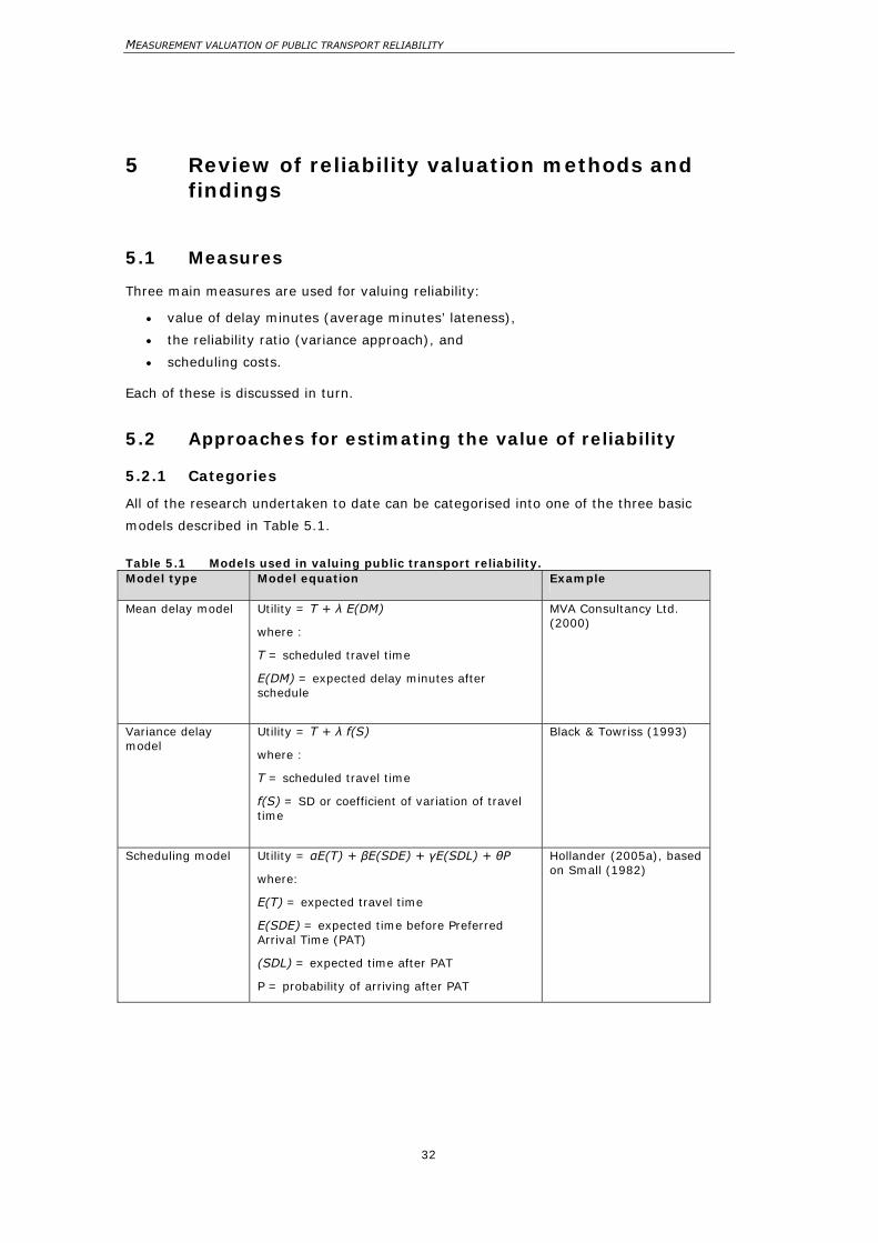
All of the research undertaken to date can be categorised into one of the three basic
models described in Table 5.1.
Table 5.1 Models used in valuing public transport reliability. Model type Model equation Example
Mean delay model Utility = T + λ E(DM)
where :
T = scheduled travel time
E(DM) = expected delay minutes after schedule
MVA Consultancy Ltd. (2000)
Variance delay model
Utility = T + λ f(S)
where :
T = scheduled travel time
f(S) = SD or coefficient of variation of travel time
Black & Towriss (1993)
Scheduling model Utility = αE(T) + βE(SDE) + γE(SDL) + θP
where:
E(T) = expected travel time
E(SDE) = expected time before Preferred Arrival Time (PAT)
(SDL) = expected time after PAT
P = probability of arriving after PAT
Hollander (2005a), based on Small (1982)
5. Review of reliability methods and findings
33
5.2.2 The mean delay approach
The mean delay approach incorporates either delays or expected delays into the
estimated utility function. The approach focuses on delays relative to schedule and
therefore is only applicable to public transport.
The value of delay minutes (or average minutes’ lateness) is discovered by calculating the
amount that people will pay to avoid a given probability of a delay of a given size. This
willingness to pay is then corresponded to average minutes saved. For example, suppose
commuters are willing to pay $0.50 to avoid a 1 in 10 probability of 10 minutes’ delay.
The average minutes saved would be (1/10) x 10 = 1. Therefore, each delay minute has
a value of $0.50 (or $30/hour).
The value of delay minutes can vary, depending on the level of risk. For example, BECA
(2002) found that delay minutes were valued at:
• $1.30/minute for a 1/5 probability of delay, and
• $1.06/minute for a 1/10 probability of delay.
Values of delay minutes are normally associated with models that represent mean delay
using data given as the probability of delay.
5.2.3 The variance delay approach
The variance delay approach attempts to value variability in travel times explicitly by
incorporating it into an estimated utility function. The main measures of variability used
are standard deviations and coefficients of variation. The variance delay approach is
commonly applied, perhaps because it is relatively easy to implement and it produces
reliability ratios.
The reliability ratio is commonly associated with studies where respondents are presented
with representative trips in a stated preference format. To calculate the reliability ratio,
researchers estimate a utility function and then divide the coefficient on the standard
deviation of travel time (generally) by the coefficient of travel time. The reliability ratio
can be easily used to value improvements in transport reliability.
However, it is interesting to note that MVA Consultancy Ltd. (2000) used a probability of
delay representation and were still able to estimate reliability ratios. But to do this, the
researchers would have had to assume an underlying distribution for the data. In
addition, the researchers were making the presumption that early arrivals have zero value
(or cost) to travellers.
MEASUREMENT VALUATION OF PUBLIC TRANSPORT RELIABILITY
34
5.2.4 The scheduling cost approach
The scheduling cost approach directs attention away from actual variability and towards
the costs of variability, i.e. the costs associated with being early or late.
The scheduling cost approach presents respondents with a Preferred Arrival Time (PAT)
(e.g. a time when they want to be at their destination) and gives them a choice of
alternatives. Each alternative has different implications for the respondent’s arrival
relative to their preferred arrival time. The scheduling cost approach uses their responses
to infer the cost associated with being early or late to the destination.
The scheduling cost approach is often preferred in academic studies because it has strong
theoretical grounds and perhaps because it focuses on the main reasons why travellers
value reliability: they want to get to work on time without leaving home too early.
However, the scheduling cost approach only produces values of ‘early time’ and ‘late time’
relative to preferred arrival times. As Bates et al. (2001) note, obtaining a ‘value of
reliability’ would require additional work: researchers would need to simulate the impact
of changes in variability on people’s arrival times and then calculate the cost of those
changes in arrival times using their estimated values of ‘early time’ and ‘late time’.
Additional information on people’s preferred arrival times would also be required in order
to do this.
To calculate scheduling costs, the researcher presents respondents with alternate options
with different schedules of representative travel tips. Each option will have different
scheduling costs. For example, one option might get the commuter to work early by ten
minutes on average; the other option might get the commuter to work late by five
minutes on average.
Based on commuters’ stated preferences, the researcher infers the likely value associated
with:
• a minute of earliness (minutes before preferred arrival time), and
• a minute of lateness (minutes after arrival time).
The researcher can also incorporate non-linearities into the estimation method. It is
common for researchers to add a ‘penalty’ based on the likelihood of being late by any
amount of time. Other non-linearities can also be accommodated.
Values of mean delay have been estimated using scheduling models (Bates et al. 2001).
However, detailed information about the distribution of passengers’ preferred arrival
times are required, and this can be problematic.
5. Review of reliability methods and findings
35
5.3 Estimating utility functions using Logit models
Most reliability studies estimate utility functions using Logit models. Estimating reliability
ratios (variance delay model) and value of delay minutes (average minutes’ lateness) is
generally quite straightforward: both the change in reliability and the change in travel-
time are entered into the utility functions, and the estimated reliability coefficient is
divided by the estimated travel-time coefficient so a relative valuation can be obtained.
Estimating the scheduling costs involves a few (minor) additional steps: the researcher
must create variables to represent scheduling costs (for example, expected minutes early,
expected minutes late and a variable representing the proportion of trips that are late).
Changes in the levels of those scheduling cost variables (compared with a distribution of
preferred arrival times) are then incorporated into the utility functions.
5.4 Valuation findings
5.4.1 Valuations in the literature
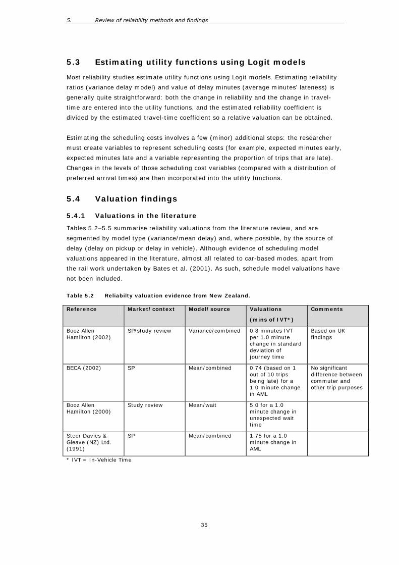
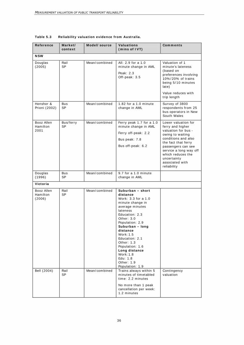
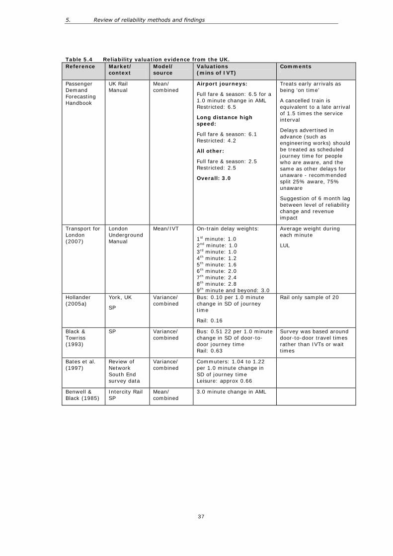
Tables 5.2–5.5 summarise reliability valuations from the literature review, and are
segmented by model type (variance/mean delay) and, where possible, by the source of
delay (delay on pickup or delay in vehicle). Although evidence of scheduling model
valuations appeared in the literature, almost all related to car-based modes, apart from
the rail work undertaken by Bates et al. (2001). As such, schedule model valuations have
not been included.
Table 5.2 Reliabilty valuation evidence from New Zealand.
* IVT = In-Vehicle Time
Reference Market/context Model/source Valuations
(mins of IVT*)
Comments
Booz Allen Hamilton (2002)
SP/study review Variance/combined
0.8 minutes IVT per 1.0 minute change in standard deviation of journey time
Based on UK findings
BECA (2002) SP Mean/combined 0.74 (based on 1 out of 10 trips being late) for a 1.0 minute change in AML
No significant difference between commuter and other trip purposes
Booz Allen Hamilton (2000)
Study review Mean/wait 5.0 for a 1.0 minute change in unexpected wait time
Steer Davies & Gleave (NZ) Ltd. (1991)
SP Mean/combined 1.75 for a 1.0 minute change in AML
MEASUREMENT VALUATION OF PUBLIC TRANSPORT RELIABILITY
36
Table 5.3 Reliability valuation evidence from Australia. Reference Market/
context Model/source Valuations
(mins of IVT) Comments
NSW
Douglas (2005)
Rail SP
Mean/combined All: 2.9 for a 1.0 minute change in AML
Peak: 2.3 Off-peak: 3.5
Valuation of 1 minute’s lateness (based on preferences involving 10%/20% of trains being 5/10 minutes late)
Value reduces with trip length
Hensher & Prioni (2002)
Bus SP
Mean/combined 1.82 for a 1.0 minute change in AML
Survey of 3800 respondents from 25 bus operators in New South Wales
Booz Allen Hamilton 2001
Bus/ferry SP
Mean/combined Ferry peak 1.7 for a 1.0 minute change in AML
Ferry off-peak: 2.2
Bus peak: 7.8
Bus off-peak: 6.2
Lower valuation for ferry and higher valuation for bus - owing to waiting conditions and also the fact that ferry passengers can see service a long way off which reduces the uncertainty associated with reliability
Douglas (1996)
Bus SP
Mean/combined 9.7 for a 1.0 minute change in AML
Victoria
Booz Allen Hamilton (2006)
Rail SP
Mean/combined Suburban – short distance Work: 3.3 for a 1.0 minute change in average minutes lateness Education: 2.3 Other: 3.0 Population: 2.9 Suburban – long distance Work:1.5 Education: 2.1 Other: 1.3 Population: 1.6 Long distance Work:1.8 Edu: 1.8 Other: 1.9 Population: 1.9
Bell (2004) Rail SP
Mean/combined Trains always within 5 minutes of timetabled time: 2.2 minutes
No more than 1 peak cancellation per week: 1.2 minutes
Contingency valuation
5. Review of reliability methods and findings
37
Table 5.4 Reliability valuation evidence from the UK. Reference Market/
context Model/ source
Valuations (mins of IVT)
Comments
Passenger Demand Forecasting Handbook
UK Rail Manual
Mean/ combined
Airport journeys:
Full fare & season: 6.5 for a 1.0 minute change in AML Restricted: 6.5
Long distance high speed:
Full fare & season: 6.1 Restricted: 4.2
All other:
Full fare & season: 2.5 Restricted: 2.5
Overall: 3.0
Treats early arrivals as being ‘on time’
A cancelled train is equivalent to a late arrival of 1.5 times the service interval
Delays advertised in advance (such as engineering works) should be treated as scheduled journey time for people who are aware, and the same as other delays for unaware - recommended split 25% aware, 75% unaware
Suggestion of 6 month lag between level of reliability change and revenue impact
Transport for London (2007)
London Underground Manual
Mean/IVT On-train delay weights:
1st minute: 1.0 2nd minute: 1.0 3rd minute: 1.0 4th minute: 1.2 5th minute: 1.6 6th minute: 2.0 7th minute: 2.4 8th minute: 2.8 9th minute and beyond: 3.0
Average weight during each minute
LUL
Hollander (2005a)
York, UK
SP
Variance/ combined
Bus: 0.10 per 1.0 minute change in SD of journey time
Rail: 0.16
Rail only sample of 20
Black & Towriss (1993)
SP Variance/ combined
Bus: 0.51 22 per 1.0 minute change in SD of door-to-door journey time Rail: 0.63
Survey was based around door-to-door travel times rather than IVTs or wait times
Bates et al. (1997)
Review of Network South End survey data
Variance/ combined
Commuters: 1.04 to 1.22 per 1.0 minute change in SD of journey time Leisure: approx 0.66
Benwell & Black (1985)
Intercity Rail SP
Mean/ combined
3.0 minute change in AML
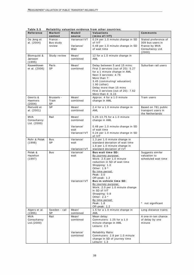
MEASUREMENT VALUATION OF PUBLIC TRANSPORT RELIABILITY
38
Table 5.5 Reliability valuation evidence from other countries. Reference Market/
context Model/ source
Valuations (mins of IVT)
Comments
De Jong et al. (2004)
France - Bus study review
Variance/IVT Variance/ Wait
0.24 per 1.0 minute change in SD of IVT 0.48 per 1.0 minute change in SD of wait time
Stated preference of 309 bus users in France by MVA Consultancy Ltd. (2000)
Blomquist & Jansson (1995)
Study review Mean/ combined
12 for a 1.0 minute change in AML
Kouwenhoven et al. (2006)
Paris SP
Mean/ combined
Delay between 5 and 15 mins: First 3 services (out of 20): 5.27 for a 1 minute change in AML Next 3 services: 4.76 More than 7: 3.45 (commuting/ education) 1.90 (other) Delay more than 15 mins First 3 services (out of 20): 7.62 More than 4: 6.15
Suburban rail users
Geerts & Haemers (2004)
Brussels - Tram SP
Mean/ combined
Approx. 4 for a 1.0 minute change in AML
Tram users
Rietveld et al. (2001)
SP Mean/ combined
2.4 for a 1.0 minute change in AML
Based on 781 public transport users in the Netherlands
MVA Consultancy Ltd. (2000)
Rail Mean/ combined Variance/ wait Variance/IVT
5.25-13.75 for a 1.0 minute change in AML 0.48 per 1.0 minute change in SD of wait time 0.24 per 1.0 minute change in SD of IVT
Rohr & Polak (1998)
Bus SP
Variance/ wait Variance/IVT
1.3 per 1.0 minute change in standard deviation of wait time 1.6 per 1.0 minute change in standard deviation of IVT
Polak & Hazelton (1997)
Bus Variance/ wait Variance/IVT
Bus wait time SD: By journey purpose: Work: 2.5 per 1.0 minute reduction in SD of wait time Shopping: 1.0 Other: 1.9 * By time period: Peak: 3.0 Off-peak: 1.2 Bus in-vehicle time SD: By journey purpose: Work: 2.0 per 1.0 minute change in SD of IVT Shopping: 0.8 Other: 2.3 * By time period: Peak: 1.8 Off-peak: 1.2
Suggests similar valuation to scheduled wait time * not significant
Algers et al. (1995)
Sweden - rail SP
Mean/ combined
1.5 for a 1.0 minute change in AML
Long distance trains
MVA Consultancy Ltd.(2000)
Rail Mean/ combined Variance/ combined
Mean delay: Commuters: 1.25 for a 1.0 minute change in AML Leisure: 2.5 Reliability Ratio: Commuters: 2.8 per 1.0 minute change in SD of journey time Leisure: 1.3
A one-in-ten chance of delay by one minute
5. Review of reliability methods and findings
39
5.4.2 Mean delay valuations
Evidence for mean delay valuations is more extensive than variance delay, and has, in
some cases, been segmented by mode and trip purpose. Sources range from individual
local studies, using mostly SP approaches, through to guidelines and handbooks with
recommended approaches/parameters.
Most valuations are not explicit about the source of the delay (whether it be delay on
passenger pickup or delay while in the vehicle), and tend to represent delay as the overall
impact if a service is late/early. The evidence that does exist suggests passengers value
delay while waiting higher than delay when on the vehicle. Booz Allen Hamilton (2000)
recommends a fivefold weighting for unexpected wait time, whilst the Transport for
London Business Case Development Manual (Transport for London 2007) recommends
weightings ranging from 1 to 3 times that of in-vehicle delay.
Overall, the average of the studies listed above suggests that an average minute’s delay
is worth four minutes of IVT, with a higher valuation for passengers picked up later and a
lower valuation for passengers already on the vehicle. A large range has been noted
across sources, with valuations as high as 13.75. No consistent relative valuations of peak
v. off-peak, bus v. rail, or trip purpose have been made, which suggests that reliability
valuations, when segmented, are very context-specific. It should also be noted that
people who value reliability highly are likely to use choose modes that are more reliable.
5.4.3 Variance delay valuations
Whilst less evidence is available for variance of delay valuations, the studies that exist
tend to provide more insight into the relative importance of pickup v. IVT variations.
Overall, an average reliability ratio of around 1 is seen in the studies, meaning a one
minute change in the variation (standard deviation) of delay is valued the same as one
minute of IVT. The evidence also suggests variation of wait times is valued around 20%
higher than variation of IVT. As with the mean delay valuations, the range of valuations is
large, up to 2.8 times IVT and as low as 0.1 times IVT, with little evidence of consistence
differences between modes and trip purposes.
5.4.4 Valuation summary
Examination of reliability attribute valuations suggests large variations, indicating the
valuations to be highly context-specific. On average, one minute of average lateness is
valued at around 4 times IVT. In terms of variability of service reliability, the evidence
suggests one minute of standard deviation of lateness is worth one minute of IVT.
Valuations for waiting passengers are generally higher than for passengers on the service.
Little evidence suggests any consistent differences by mode, time of day or trip purpose.
MEASUREMENT VALUATION OF PUBLIC TRANSPORT RELIABILITY
40
6 Reliability SP survey
6.1 Possible approaches
As discussed in Chapter 4, in general, two methods for determining passengers’ valuation
of reliability exist: revealed preference and stated preference approaches. The lack of
consistent patronage data when reliability improvements occurred meant that revealed
preference methods could not be used in this study. As such, a stated preference survey
was undertaken to determine passengers’ preferences for different levels of reliability and
other related issues.
This chapter outlines the development of the survey, particularly the thought processes
that contributed to the final design. The survey process is discussed, including pilot
surveys and findings.
6.2 Why does reliability matter?
Chapter 2 outlines some of the issues that public transport users face when using an
unreliable service. In particular, public transport users are concerned about lateness on
arrival at their destination, which can be caused by unreliability both at pickup and during
the trip. A cost is also associated with early services as passengers get distressed – they
do not know if they have missed the service or if, having missed their preferred service,
they are required to wait for the next. For passengers that are on the service, however,
early running could be viewed as a benefit because of the reduced journey times. In
general, passengers are irritated by a service that does not follow its schedule.
As such, any developed survey needs to explore late and early running services for bus
and train modes. Ideally, it should explore the effect of delay in waiting for services
(unexpected wait time) and delay en route.
6. Reliability SP survey
41
6.3 Parameter valuation
A review of reliability methodology frameworks in Chapter 5 identified three main
measures used for valuing reliability:
• the value of delay minutes (AML),
• the reliability ratio (variance delay approach), and
• the scheduling model.
A scheduling model (variability relative to a preferred arrival time) was not chosen as the
preferred valuation methodology, primarily because a distribution of preferred arrival
times in many cases needs to be assumed – and, as such, limits the usefulness of the
approach.
The structure of a delay model SP survey (variability relative to a schedule) can be used
to examine both a reliability ratio and a valuation of delay minutes, as the contained
variables are applicable to both forms. Furthermore, a delay approach has other benefits:
• it can be used focus on non-linearities in the value of lateness;
• is is easier to implement, as passenger impacts can be determined from service
statistics without the need for passengers’ preferred arrival times; and
• it is an easier concept for respondents to understand.
Another advantage of the delay model is that standard deviation around average lateness
may be important. For example, passengers might be happy with a service that is
consistently late as they can change their trip behaviour accordingly (e.g. always arriving
at the service five minutes later than the scheduled time). As a further illustration, both
distributions below have the same mean delay (disregarding non-linearities) but the first
distribution might be preferred because it has the smaller standard deviation:
2 2 2 2 2 mean delay = 2, SD =0
0 0 0 0 10 mean delay = 2, SD = 4.5
Therefore, to the extent possible, the SP exercises were designed so that any combination
of mean delays or standard deviations could be explored. The research could fit a model
with mean delays only, standard deviation only or a combination of both.
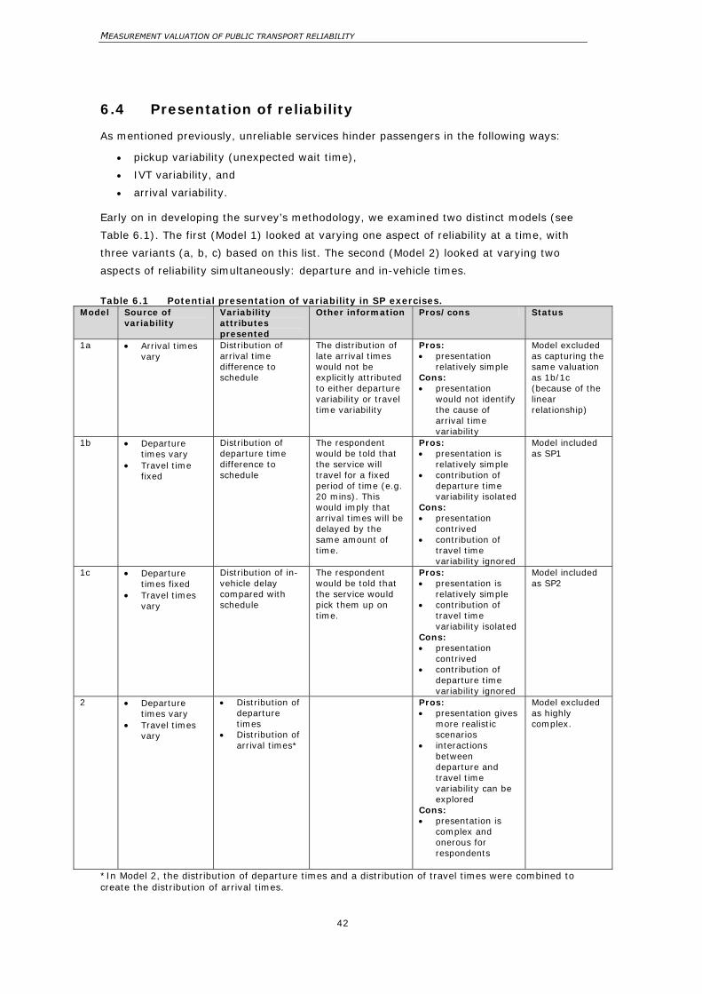
MEASUREMENT VALUATION OF PUBLIC TRANSPORT RELIABILITY
42
6.4 Presentation of reliability
As mentioned previously, unreliable services hinder passengers in the following ways:
• pickup variability (unexpected wait time),
• IVT variability, and
• arrival variability.
Early on in developing the survey’s methodology, we examined two distinct models (see
Table 6.1). The first (Model 1) looked at varying one aspect of reliability at a time, with
three variants (a, b, c) based on this list. The second (Model 2) looked at varying two
aspects of reliability simultaneously: departure and in-vehicle times.
Table 6.1 Potential presentation of variability in SP exercises.
Model Source of variability
Variability attributes presented
Other information Pros/cons Status
1a • Arrival times vary
Distribution of arrival time difference to schedule
The distribution of late arrival times would not be explicitly attributed to either departure variability or travel time variability
Pros: • presentation
relatively simple Cons: • presentation
would not identify the cause of arrival time variability
Model excluded as capturing the same valuation as 1b/1c (because of the linear relationship)
1b • Departure times vary
• Travel time fixed
Distribution of departure time difference to schedule
The respondent would be told that the service will travel for a fixed period of time (e.g. 20 mins). This would imply that arrival times will be delayed by the same amount of time.
Pros: • presentation is
relatively simple • contribution of
departure time variability isolated
Cons: • presentation
contrived • contribution of
travel time variability ignored
Model included as SP1
1c • Departure times fixed
• Travel times vary
Distribution of in-vehicle delay compared with schedule
The respondent would be told that the service would pick them up on time.
Pros: • presentation is
relatively simple • contribution of
travel time variability isolated
Cons: • presentation
contrived • contribution of
departure time variability ignored
Model included as SP2
2 • Departure times vary
• Travel times vary
• Distribution of departure times
• Distribution of arrival times*
Pros: • presentation gives
more realistic scenarios
• interactions between departure and travel time variability can be explored
Cons: • presentation is
complex and onerous for respondents
Model excluded as highly complex.
*In Model 2, the distribution of departure times and a distribution of travel times were combined to create the distribution of arrival times.
6. Reliability SP survey
43
Model 2 (varying departure and in-vehicle reliability simultaneously) was excluded early in
the process because of the complexity of the survey design. Varying both would require
complex trade-offs by the respondents, and might result in confusion and unrealistic
trading between services. It was decided that the simpler approach of examining one
aspect of reliability at a time was more desirable. Model 1a was then excluded as arrival
time variation is a result of either delay at pickup or delay en route (arrival time =
departure time + travel time), and these would be captured by Models 1b and 1c.
It was decided to take Models 1b and 1c forward as part of the survey process. These
would form two SP surveys that each respondent would be asked to complete. The first
related to departure time reliability; the second, IVT reliability.
We decided to present reliability in terms of the number of services (out of 10) 5 minutes
early, the number that were 5 minutes late and the number that were 10 minutes late.
The level of reliability (numbers presented) was varied between scenarios, and was fixed
for all respondents.
The SP survey was designed to provide valuations for earliness, being 5 minutes late and
being 10 minutes late. Our initial hypothesis was:
• Early departure time would be valued highly because of the risk that some
passengers would miss a service.
• Reduced (‘early’) IVT is likely to have a lower valuation, as some passengers may
see the reduction in travel time as a bonus.
• Five minutes’ lateness should have a higher valuation than IVT but also have a
lower valuation than ten minutes’ lateness or ten minutes’ earliness.
MEASUREMENT VALUATION OF PUBLIC TRANSPORT RELIABILITY
44
6.5 SP survey design
The questionnaire design is extremely important, particularly in SP surveys where
respondents are usually asked about complex hypothetical situations. The information
needs to be relayed to respondents in a clear and concise manner so that the decision
making process is as simple as possible.
An SP showcard gives a respondent the choice between two scenarios with differing levels
of reliability and travel characteristics. Generally, the respondent trades off a more
reliable, more expensive and shorter scheduled time service against a less
reliable/cheaper/longer service. How the respondent trades gives an indication of the
value they place on reliability, cost and travel time.
To encourage respondents to trade, the showcards presented need to have sufficient
variation, while still providing realistic options. Variation can be controlled by the number
of levels presented for each variable and by the tolerance around a central value. The
central value (for scheduled travel time and fare) is based on the respondents’ current
trip-making characteristics so as to provide realistic alternatives. The number of levels is
based on the number of showcards that are to be presented and the number of variables
included. The more showcards presented, the richer the dataset; however, the longer the
survey, the higher the chances of fatigue.
The project team decided to use a 16 showcard design for each of the two SPs (32 cards
in total). Both SPs were then split in half, with each respondent being asked to respond to
8 cards from each SP (a total of 16 cards per respondent), as it was felt that 32 cards
would be too onerous for an individual.
The design for the departure time variability survey would include five variables:
• scheduled trip time (at 4 levels),
• trip fare (at 4 levels),
• the number of trips about 5 minutes early on departure (at 3 levels),
• the number of trips about 5 minutes late on departure (at 3 levels), and
• the number of trips about 10 minutes late on departure (at 3 levels),
The in-vehicle time variability survey would include 4 variables:
• trip fare (at 4 levels)
• the number of trips about 5 minutes early whilst on service (at 3 levels),
• the number of trips about 5 minutes late whilst on service (at 3 levels), and
• the number of trips about 10 minutes late whilst on service (at 3 levels).
Scheduled travel time (not included in the IVT SP survey) and fare paid were both
included in the SP survey as well as the reliability variable. The inclusion of fare (in
addition to minutes of IVT) was recommended because it enables the estimation of a
value of time (which is a useful ‘check’ on the validity of the survey), it disguises the
trade-offs from the respondent to the SP survey, and prevented ‘over-rationalisation’.
6. Reliability SP survey
45
Scheduled travel time was excluded from the in-vehicle survey as it was felt that including
in-vehicle time then varying in-vehicle time would confuse respondents.
The inclusion of headway (as an attribute) was avoided for two reasons:
• frequency can overwhelm the other attributes and reduce the accuracy of estimates
of the other attributes; and
• hypothetical changes in frequency can confuse the respondent. For example, a
service that is halved in frequency will mean that the respondent has a 50% chance
of catching the bus that they currently catch – communicating this to respondents
would be very difficult.
Respondents were asked to assume that services ran as frequently as they currently do.
Although headway was not included as an attribute, the headway of the respondent’s
current service was recorded. The headway of the respondent’s current service could then
be used as an explanatory variable if further analysis was required.
The levels on the showcard were presented in such a way that the experiment was
orthogonal. The in-vehicle time SP included the same variables and number of levels, but
trip time was excluded as it was felt that including this (at varying levels) would cause
confusion if trip time was changed for reliability reasons.
Differing approaches have been used to represent reliability in SP surveys with varying
degrees of success (see Chapters 4.2 and 4.3). The following representation mechanisms
were considered:
• the clockface design,
• the bar-chart design,
• the pie-chart design, and
• text descriptions.
The standard method used in the literature is a set of representative trips using either a
clockface design or bar-chart design. In the end, the combination of a bar-chart (but
using pictures of vehicles) and text descriptions were used to outline the scenarios
presented in the showcards (see
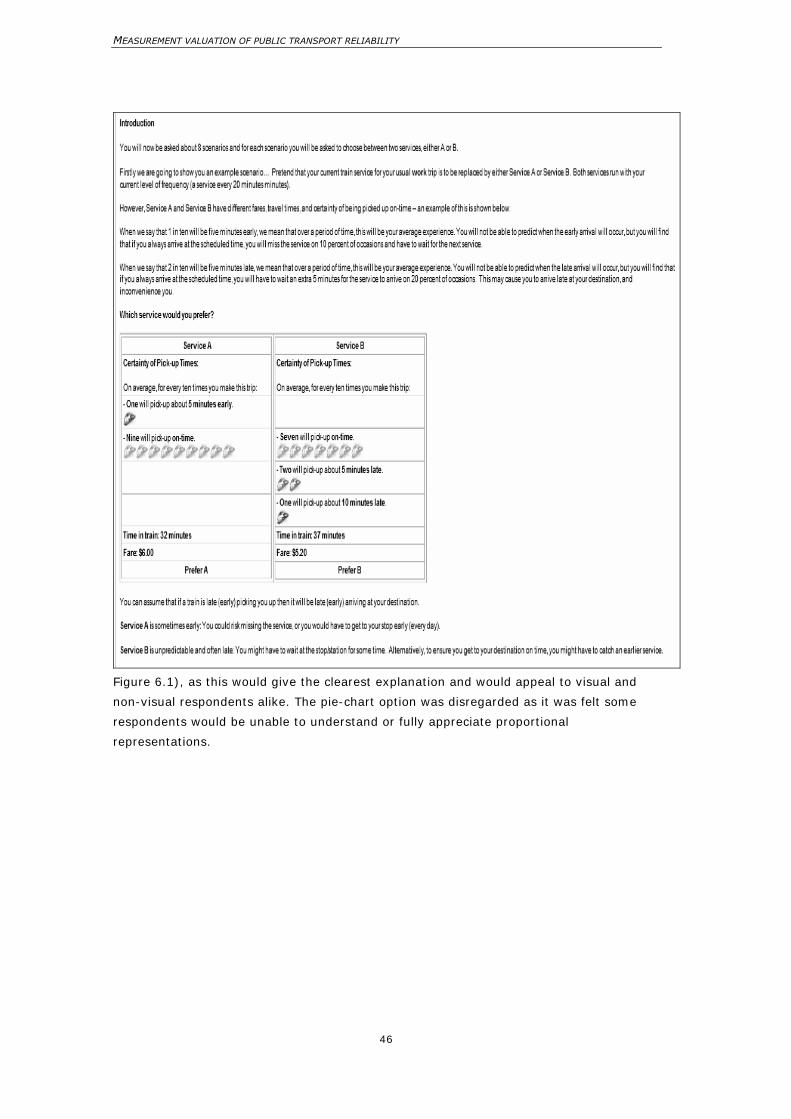
MEASUREMENT VALUATION OF PUBLIC TRANSPORT RELIABILITY
46
Figure 6.1), as this would give the clearest explanation and would appeal to visual and
non-visual respondents alike. The pie-chart option was disregarded as it was felt some
respondents would be unable to understand or fully appreciate proportional
representations.
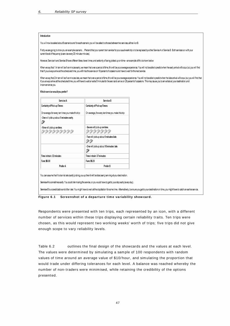
6. Reliability SP survey
47
Figure 6.1 Screenshot of a departure time variability showcard.
Respondents were presented with ten trips, each represented by an icon, with a different
number of services within these trips displaying certain reliability traits. Ten trips were
chosen, as this would represent two working weeks’ worth of trips; five trips did not give
enough scope to vary reliability levels.
Table 6.2 outlines the final design of the showcards and the values at each level.
The values were determined by simulating a sample of 100 respondents with random
values of time around an average value of $10/hour, and simulating the proportion that
would trade under differing tolerances for each level. A balance was reached whereby the
number of non-traders were minimised, while retaining the credibility of the options
presented.
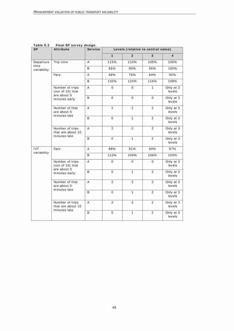
MEASUREMENT VALUATION OF PUBLIC TRANSPORT RELIABILITY
48
Table 6.2 Final SP survey design.
Levels (relative to central value) SP Attribute Service
1 2 3 4
A 115% 110% 105% 100% Trip time
B 85% 90% 95% 100%
A 68% 76% 84% 92% Fare
B 132% 124% 116% 108%
A 0 0 1 Only at 3 levels
Number of trips (out of 10) that are about 5 minutes early B 0 0 0 Only at 3
levels
A 2 2 2 Only at 3 levels
Number of that are about 5 minutes late
B 0 1 2 Only at 3 levels
A 2 2 2 Only at 3 levels
Departure time variability
Number of trips that are about 10 minutes late
B 0 1 2 Only at 3 levels
A 88% 91% 94% 97% Fare
B 112% 109% 106% 103%
A 0 0 0 Only at 3 levels
Number of trips (out of 10) that are about 5 minutes early B 0 1 2 Only at 3
levels
A 2 2 2 Only at 3 levels
Number of that are about 5 minutes late
B 0 1 2 Only at 3 levels
A 2 2 2 Only at 3 levels
IVT variability
Number of trips that are about 10 minutes late
B 0 1 2 Only at 3 levels
6. Reliability SP survey
49
6.6 Survey delivery
6.6.1 Recruitment and delivery
A survey specification was provided to the market research company. The target
population was defined as:
‘All bus users in Auckland and Wellington, and all train users in Wellington.’
The survey was conducted online using SmileCity, and was customisable to a user’s
response (particularly their current trip-making behaviour). SmileCity has an online
membership pool of around 130 000 users, who earn rewards by completing online
surveys.
6.6.2 Sample size and selection
It was decided that quotas were required so that reasonable results could be estimated
when the market was segmented (See Table 6.3). The segments decided on were
geography (Auckland/Wellington), mode (bus/train) and trip purpose
(work/education/other). The pilot showed that education trip purposes would provide the
biggest recruitment challenge, so the quotas for these segments were set lower. Also, a
priority selection (education, work then other) was initiated whereby if a respondent had
used public transport for several purposes, then the segments that would be hardest to
obtain would be sampled first. This meant that the sample obtained as part of this study
is not a random sample.
Respondents were only selected if they lived in Auckland or Wellington, and if they had
made a return trip on public transport in the last month. Very occasional users of public
transport were not included in the sample, as they would be unlikely to provide realistic
insights into reliability.
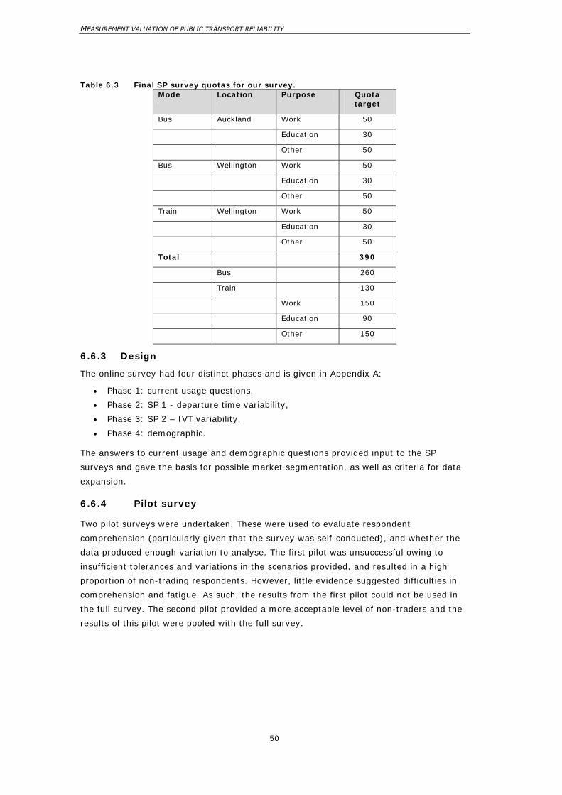
MEASUREMENT VALUATION OF PUBLIC TRANSPORT RELIABILITY
50
Table 6.3 Final SP survey quotas for our survey. Mode Location Purpose Quota
target
Bus Auckland Work 50
Education 30
Other 50
Bus Wellington Work 50
Education 30
Other 50
Train Wellington Work 50
Education 30
Other 50
Total 390
Bus 260
Train 130
Work 150
Education 90
Other 150
6.6.3 Design
The online survey had four distinct phases and is given in Appendix A:
• Phase 1: current usage questions,
• Phase 2: SP 1 - departure time variability,
• Phase 3: SP 2 – IVT variability,
• Phase 4: demographic.
The answers to current usage and demographic questions provided input to the SP
surveys and gave the basis for possible market segmentation, as well as criteria for data
expansion.
6.6.4 Pilot survey
Two pilot surveys were undertaken. These were used to evaluate respondent
comprehension (particularly given that the survey was self-conducted), and whether the
data produced enough variation to analyse. The first pilot was unsuccessful owing to
insufficient tolerances and variations in the scenarios provided, and resulted in a high
proportion of non-trading respondents. However, little evidence suggested difficulties in
comprehension and fatigue. As such, the results from the first pilot could not be used in
the full survey. The second pilot provided a more acceptable level of non-traders and the
results of this pilot were pooled with the full survey.
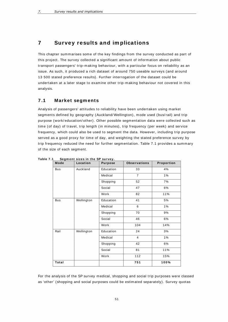
7. Survey results and implications
51
7 Survey results and implications
This chapter summarises some of the key findings from the survey conducted as part of
this project. The survey collected a significant amount of information about public
transport passengers’ trip-making behaviour, with a particular focus on reliability as an
issue. As such, it produced a rich dataset of around 750 useable surveys (and around
13 500 stated preference results). Further interrogation of the dataset could be
undertaken at a later stage to examine other trip-making behaviour not covered in this
analysis.
7.1 Market segments
Analysis of passengers’ attitudes to reliability have been undertaken using market
segments defined by geography (Auckland/Wellington), mode used (bus/rail) and trip
purpose (work/education/other). Other possible segmentation data were collected such as
time (of day) of travel, trip length (in minutes), trip frequency (per week) and service
frequency, which could also be used to segment the data. However, including trip purpose
served as a good proxy for time of day, and weighting the stated preference survey by
trip frequency reduced the need for further segmentation. Table 7.1 provides a summary
of the size of each segment.
Table 7.1 Segment sizes in the SP survey.
Mode Location Purpose Observations Proportion
Education 33 4%
Medical 7 1%
Shopping 52 7%
Social 47 6%
Bus Auckland
Work 82 11%
Education 41 5%
Medical 6 1%
Shopping 70 9%
Social 46 6%
Bus Wellington
Work 104 14%
Education 24 3%
Medical 4 1%
Shopping 42 6%
Social 81 11%
Rail Wellington
Work 112 15%
Total 751 100%
For the analysis of the SP survey medical, shopping and social trip purposes were classed
as ‘other’ (shopping and social purposes could be estimated separately). Survey quotas
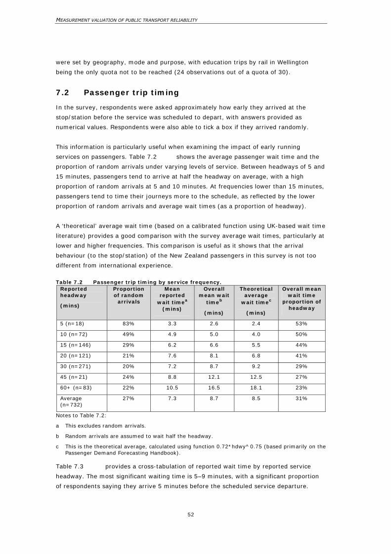
MEASUREMENT VALUATION OF PUBLIC TRANSPORT RELIABILITY
52
were set by geography, mode and purpose, with education trips by rail in Wellington
being the only quota not to be reached (24 observations out of a quota of 30).
7.2 Passenger trip timing
In the survey, respondents were asked approximately how early they arrived at the
stop/station before the service was scheduled to depart, with answers provided as
numerical values. Respondents were also able to tick a box if they arrived randomly.
This information is particularly useful when examining the impact of early running
services on passengers. Table 7.2 shows the average passenger wait time and the
proportion of random arrivals under varying levels of service. Between headways of 5 and
15 minutes, passengers tend to arrive at half the headway on average, with a high
proportion of random arrivals at 5 and 10 minutes. At frequencies lower than 15 minutes,
passengers tend to time their journeys more to the schedule, as reflected by the lower
proportion of random arrivals and average wait times (as a proportion of headway).
A ‘theoretical’ average wait time (based on a calibrated function using UK-based wait time
literature) provides a good comparison with the survey average wait times, particularly at
lower and higher frequencies. This comparison is useful as it shows that the arrival
behaviour (to the stop/station) of the New Zealand passengers in this survey is not too
different from international experience.
Table 7.2 Passenger trip timing by service frequency.
Reported headway
(mins)
Proportion of random
arrivals
Mean reported
wait timea (mins)
Overall mean wait
timeb
(mins)
Theoretical average
wait timec
(mins)
Overall mean wait time
proportion of headway
5 (n=18) 83% 3.3 2.6 2.4 53%
10 (n=72) 49% 4.9 5.0 4.0 50%
15 (n=146) 29% 6.2 6.6 5.5 44%
20 (n=121) 21% 7.6 8.1 6.8 41%
30 (n=271) 20% 7.2 8.7 9.2 29%
45 (n=21) 24% 8.8 12.1 12.5 27%
60+ (n=83) 22% 10.5 16.5 18.1 23%
Average (n=732)
27% 7.3 8.7 8.5 31%
Notes to Table 7.2:
a This excludes random arrivals.
b Random arrivals are assumed to wait half the headway.
c This is the theoretical average, calculated using function 0.72*hdwy^0.75 (based primarily on the Passenger Demand Forecasting Handbook).
Table 7.3 provides a cross-tabulation of reported wait time by reported service
headway. The most significant waiting time is 5–9 minutes, with a significant proportion
of respondents saying they arrive 5 minutes before the scheduled service departure.
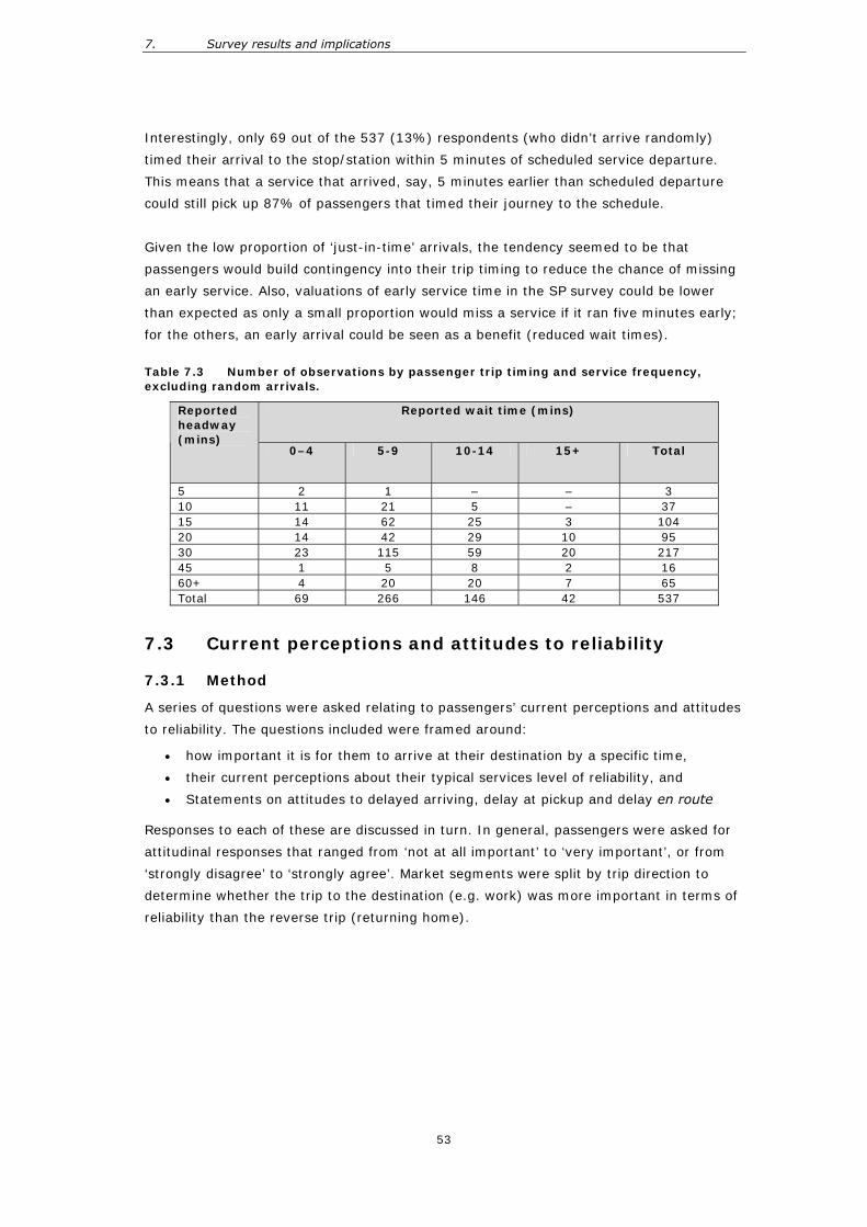
7. Survey results and implications
53
Interestingly, only 69 out of the 537 (13%) respondents (who didn’t arrive randomly)
timed their arrival to the stop/station within 5 minutes of scheduled service departure.
This means that a service that arrived, say, 5 minutes earlier than scheduled departure
could still pick up 87% of passengers that timed their journey to the schedule.
Given the low proportion of ‘just-in-time’ arrivals, the tendency seemed to be that
passengers would build contingency into their trip timing to reduce the chance of missing
an early service. Also, valuations of early service time in the SP survey could be lower
than expected as only a small proportion would miss a service if it ran five minutes early;
for the others, an early arrival could be seen as a benefit (reduced wait times).
Table 7.3 Number of observations by passenger trip timing and service frequency, excluding random arrivals.
Reported wait time (mins) Reported headway (mins)
0–4 5-9 10-14 15+ Total
5 2 1 – – 3 10 11 21 5 – 37 15 14 62 25 3 104 20 14 42 29 10 95 30 23 115 59 20 217 45 1 5 8 2 16 60+ 4 20 20 7 65 Total 69 266 146 42 537
7.3 Current perceptions and attitudes to reliability
7.3.1 Method
A series of questions were asked relating to passengers’ current perceptions and attitudes
to reliability. The questions included were framed around:
• how important it is for them to arrive at their destination by a specific time,
• their current perceptions about their typical services level of reliability, and
• Statements on attitudes to delayed arriving, delay at pickup and delay en route
Responses to each of these are discussed in turn. In general, passengers were asked for
attitudinal responses that ranged from ‘not at all important’ to ‘very important’, or from
‘strongly disagree’ to ‘strongly agree’. Market segments were split by trip direction to
determine whether the trip to the destination (e.g. work) was more important in terms of
reliability than the reverse trip (returning home).
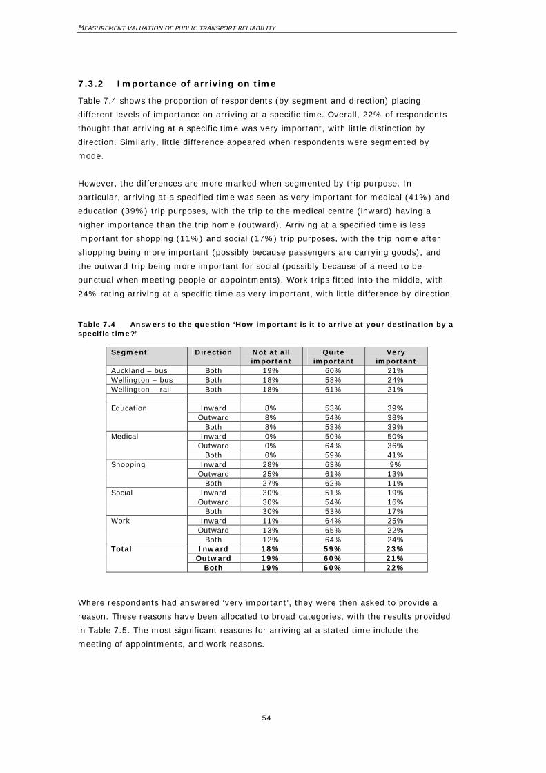
MEASUREMENT VALUATION OF PUBLIC TRANSPORT RELIABILITY
54
7.3.2 Importance of arriving on time
Table 7.4 shows the proportion of respondents (by segment and direction) placing
different levels of importance on arriving at a specific time. Overall, 22% of respondents
thought that arriving at a specific time was very important, with little distinction by
direction. Similarly, little difference appeared when respondents were segmented by
mode.
However, the differences are more marked when segmented by trip purpose. In
particular, arriving at a specified time was seen as very important for medical (41%) and
education (39%) trip purposes, with the trip to the medical centre (inward) having a
higher importance than the trip home (outward). Arriving at a specified time is less
important for shopping (11%) and social (17%) trip purposes, with the trip home after
shopping being more important (possibly because passengers are carrying goods), and
the outward trip being more important for social (possibly because of a need to be
punctual when meeting people or appointments). Work trips fitted into the middle, with
24% rating arriving at a specific time as very important, with little difference by direction.
Table 7.4 Answers to the question ‘How important is it to arrive at your destination by a specific time?’
Segment Direction Not at all important
Quite important
Very important
Auckland – bus Both 19% 60% 21% Wellington – bus Both 18% 58% 24% Wellington – rail Both 18% 61% 21%
Inward 8% 53% 39% Outward 8% 54% 38%
Education
Both 8% 53% 39% Inward 0% 50% 50%
Outward 0% 64% 36% Medical
Both 0% 59% 41% Inward 28% 63% 9%
Outward 25% 61% 13% Shopping
Both 27% 62% 11% Inward 30% 51% 19%
Outward 30% 54% 16% Social
Both 30% 53% 17% Inward 11% 64% 25%
Outward 13% 65% 22% Work
Both 12% 64% 24% Inward 18% 59% 23%
Outward 19% 60% 21% Total
Both 19% 60% 22%
Where respondents had answered ‘very important’, they were then asked to provide a
reason. These reasons have been allocated to broad categories, with the results provided
in Table 7.5. The most significant reasons for arriving at a stated time include the
meeting of appointments, and work reasons.
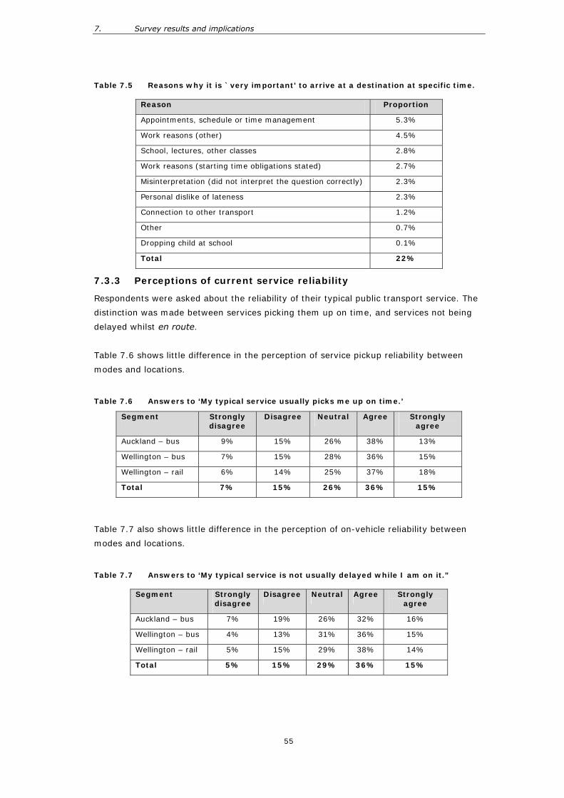
7. Survey results and implications
55
Table 7.5 Reasons why it is `very important’ to arrive at a destination at specific time.
Reason Proportion
Appointments, schedule or time management 5.3%
Work reasons (other) 4.5%
School, lectures, other classes 2.8%
Work reasons (starting time obligations stated) 2.7%
Misinterpretation (did not interpret the question correctly) 2.3%
Personal dislike of lateness 2.3%
Connection to other transport 1.2%
Other 0.7%
Dropping child at school 0.1%
Total 22%
7.3.3 Perceptions of current service reliability
Respondents were asked about the reliability of their typical public transport service. The
distinction was made between services picking them up on time, and services not being
delayed whilst en route.
Table 7.6 shows little difference in the perception of service pickup reliability between
modes and locations.
Table 7.6 Answers to ‘My typical service usually picks me up on time.’
Segment Strongly disagree
Disagree Neutral Agree Strongly agree
Auckland – bus 9% 15% 26% 38% 13%
Wellington – bus 7% 15% 28% 36% 15%
Wellington – rail 6% 14% 25% 37% 18%
Total 7% 15% 26% 36% 15%
Table 7.7 also shows little difference in the perception of on-vehicle reliability between
modes and locations.
Table 7.7 Answers to ‘My typical service is not usually delayed while I am on it.”
Segment Strongly disagree
Disagree Neutral Agree Strongly agree
Auckland – bus 7% 19% 26% 32% 16%
Wellington – bus 4% 13% 31% 36% 15%
Wellington – rail 5% 15% 29% 38% 14%
Total 5% 15% 29% 36% 15%
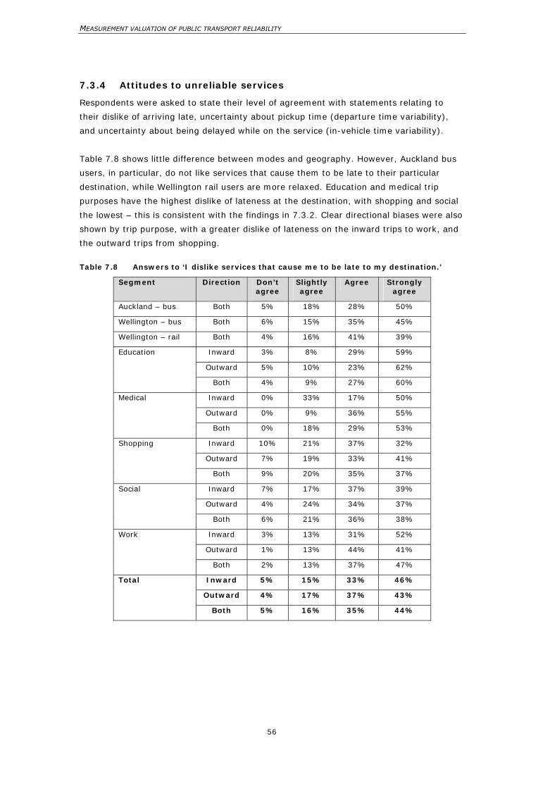
MEASUREMENT VALUATION OF PUBLIC TRANSPORT RELIABILITY
56
7.3.4 Attitudes to unreliable services
Respondents were asked to state their level of agreement with statements relating to
their dislike of arriving late, uncertainty about pickup time (departure time variability),
and uncertainty about being delayed while on the service (in-vehicle time variability).
Table 7.8 shows little difference between modes and geography. However, Auckland bus
users, in particular, do not like services that cause them to be late to their particular
destination, while Wellington rail users are more relaxed. Education and medical trip
purposes have the highest dislike of lateness at the destination, with shopping and social
the lowest – this is consistent with the findings in 7.3.2. Clear directional biases were also
shown by trip purpose, with a greater dislike of lateness on the inward trips to work, and
the outward trips from shopping.
Table 7.8 Answers to ‘I dislike services that cause me to be late to my destination.’
Segment Direction Don’t agree
Slightly agree
Agree Strongly agree
Auckland – bus Both 5% 18% 28% 50%
Wellington – bus Both 6% 15% 35% 45%
Wellington – rail Both 4% 16% 41% 39%
Inward 3% 8% 29% 59%
Outward 5% 10% 23% 62%
Education
Both 4% 9% 27% 60%
Inward 0% 33% 17% 50%
Outward 0% 9% 36% 55%
Medical
Both 0% 18% 29% 53%
Inward 10% 21% 37% 32%
Outward 7% 19% 33% 41%
Shopping
Both 9% 20% 35% 37%
Inward 7% 17% 37% 39%
Outward 4% 24% 34% 37%
Social
Both 6% 21% 36% 38%
Inward 3% 13% 31% 52%
Outward 1% 13% 44% 41%
Work
Both 2% 13% 37% 47%
Inward 5% 15% 33% 46%
Outward 4% 17% 37% 43%
Total
Both 5% 16% 35% 44%
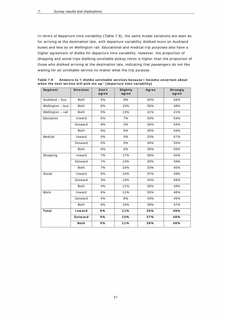
7. Survey results and implications
57
In terms of departure time variability (Table 7.9), the same modal variations are seen as
for arriving at the destination late, with departure variability disliked more on Auckland
buses and less so on Wellington rail. Educational and medical trip purposes also have a
higher agreement of dislike for departure time variability. However, the proportion of
shopping and social trips disliking unreliable pickup times is higher than the proportion of
those who disliked arriving at the destination late, indicating that passengers do not like
waiting for an unreliable service no matter what the trip purpose.
Table 7.9 Answers to ‘I dislike unreliable services because I become uncertain about when the next service will pick me up.’ (departure time variability)
Segment Direction Don’t agree
Slightly agree
Agree Strongly agree
Auckland – bus Both 5% 8% 30% 56%
Wellington – bus Both 6% 10% 36% 48%
Wellington – rail Both 5% 13% 41% 41%
Inward 5% 7% 34% 54%
Outward 8% 3% 36% 54%
Education
Both 6% 5% 35% 54%
Inward 0% 0% 33% 67%
Outward 0% 9% 36% 55%
Medical
Both 0% 6% 35% 59%
Inward 7% 17% 36% 40%
Outward 7% 13% 30% 49%
Shopping
Both 7% 15% 33% 45%
Inward 5% 10% 37% 49%
Outward 3% 13% 34% 49%
Social
Both 4% 11% 36% 49%
Inward 6% 11% 35% 48%
Outward 4% 8% 43% 45%
Work
Both 5% 10% 39% 47%
Inward 6% 11% 35% 48%
Outward 5% 10% 37% 48%
Total
Both 5% 11% 36% 48%
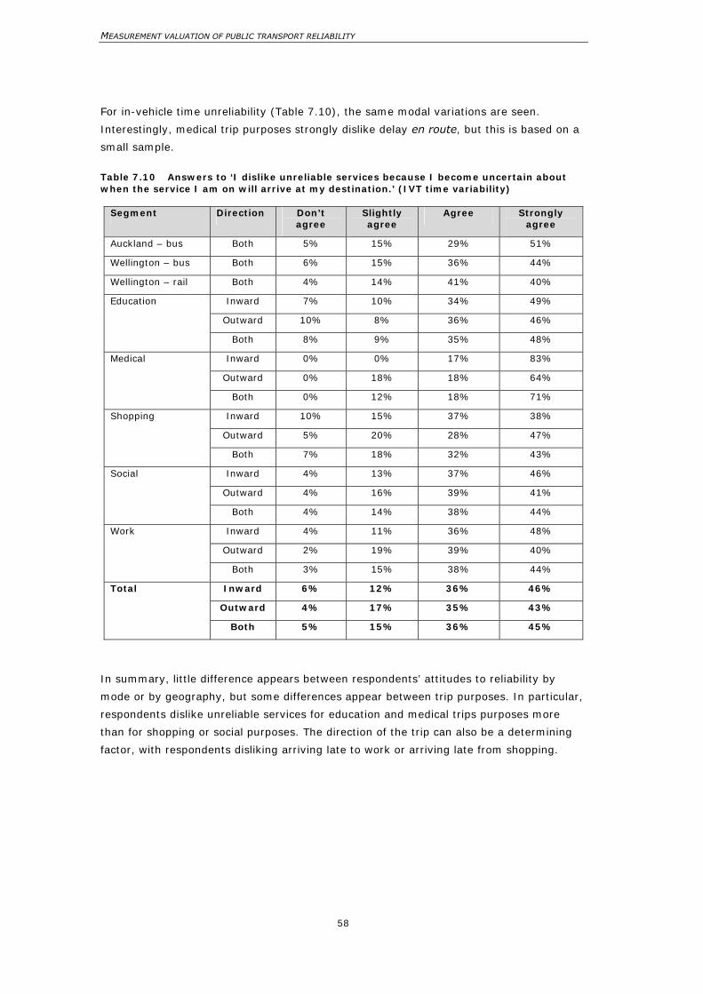
MEASUREMENT VALUATION OF PUBLIC TRANSPORT RELIABILITY
58
For in-vehicle time unreliability (Table 7.10), the same modal variations are seen.
Interestingly, medical trip purposes strongly dislike delay en route, but this is based on a
small sample.
Table 7.10 Answers to ‘I dislike unreliable services because I become uncertain about when the service I am on will arrive at my destination.’ (IVT time variability)
Segment Direction Don’t agree
Slightly agree
Agree Strongly agree
Auckland – bus Both 5% 15% 29% 51%
Wellington – bus Both 6% 15% 36% 44%
Wellington – rail Both 4% 14% 41% 40%
Inward 7% 10% 34% 49%
Outward 10% 8% 36% 46%
Education
Both 8% 9% 35% 48%
Inward 0% 0% 17% 83%
Outward 0% 18% 18% 64%
Medical
Both 0% 12% 18% 71%
Inward 10% 15% 37% 38%
Outward 5% 20% 28% 47%
Shopping
Both 7% 18% 32% 43%
Inward 4% 13% 37% 46%
Outward 4% 16% 39% 41%
Social
Both 4% 14% 38% 44%
Inward 4% 11% 36% 48%
Outward 2% 19% 39% 40%
Work
Both 3% 15% 38% 44%
Inward 6% 12% 36% 46%
Outward 4% 17% 35% 43%
Total
Both 5% 15% 36% 45%
In summary, little difference appears between respondents’ attitudes to reliability by
mode or by geography, but some differences appear between trip purposes. In particular,
respondents dislike unreliable services for education and medical trips purposes more
than for shopping or social purposes. The direction of the trip can also be a determining
factor, with respondents disliking arriving late to work or arriving late from shopping.
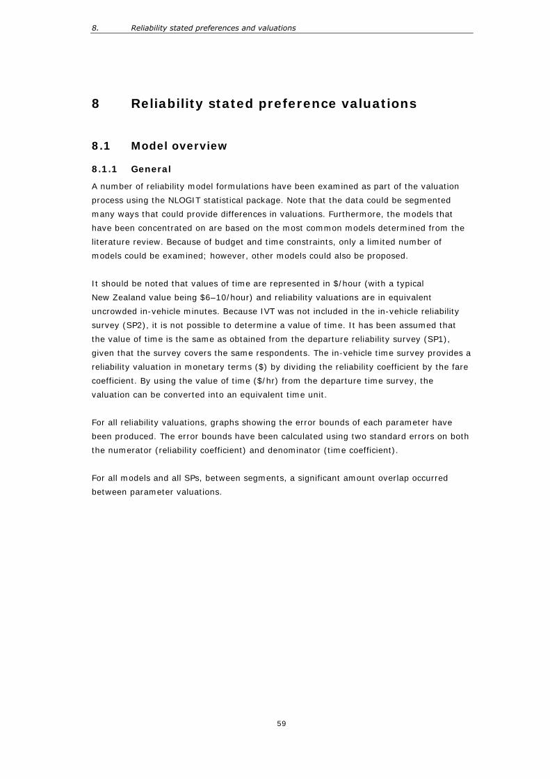
8. Reliability stated preferences and valuations
59
8 Reliability stated preference valuations
8.1 Model overview
8.1.1 General
A number of reliability model formulations have been examined as part of the valuation
process using the NLOGIT statistical package. Note that the data could be segmented
many ways that could provide differences in valuations. Furthermore, the models that
have been concentrated on are based on the most common models determined from the
literature review. Because of budget and time constraints, only a limited number of
models could be examined; however, other models could also be proposed.
It should be noted that values of time are represented in $/hour (with a typical
New Zealand value being $6–10/hour) and reliability valuations are in equivalent
uncrowded in-vehicle minutes. Because IVT was not included in the in-vehicle reliability
survey (SP2), it is not possible to determine a value of time. It has been assumed that
the value of time is the same as obtained from the departure reliability survey (SP1),
given that the survey covers the same respondents. The in-vehicle time survey provides a
reliability valuation in monetary terms ($) by dividing the reliability coefficient by the fare
coefficient. By using the value of time ($/hr) from the departure time survey, the
valuation can be converted into an equivalent time unit.
For all reliability valuations, graphs showing the error bounds of each parameter have
been produced. The error bounds have been calculated using two standard errors on both
the numerator (reliability coefficient) and denominator (time coefficient).
For all models and all SPs, between segments, a significant amount overlap occurred
between parameter valuations.
MEASUREMENT VALUATION OF PUBLIC TRANSPORT RELIABILITY
60
8.1.2 Departure time variability model
8.1.2.1 Variables
The departure time variability stated preference survey collected respondents’
preferences for particular services given changes in the following variables:
• scheduled trip time (at four levels),
• trip fare (at four levels),
• number of trips about 5 minutes early on departure (at 3 levels),
• number of trips about 5 minutes late on departure (at 3 levels), and
• number of trips about 10 minutes late on departure (at 3 levels).
Using the three reliability variables, two other variables have been calculated for use in
model estimation: average minutes’ lateness and standard deviation of lateness as
explained below.
Four models have been examined.
8.1.2.2 Model 1
This is a disaggregate model which allows valuations for departing 5 minutes early, 5
minutes late and 10 minutes late to be determined:
Utility = αT + βF + µD Early + λD Late5 + γD Late10 + constant [Equation 1]
Where: T = scheduled travel time
F = average fare
Early, Late5, Late10 = number (out of 10) of services early, 5 minutes
late, and 10 minutes late
α, β, µ, λ, γ = coefficients
The coefficients on the variables Early, Late5 and Late10 can be interpreted as the impact
of the number (N) out of ten services with the specified earliness/lateness. Since we
require valuations in the context of a single journey, it is appropriate to multiply the
estimated coefficients by ten (this effectively converts the variables ‘Early’ etc. to
probabilities. For the ‘Late’ variables, the expected lateness for each service would be the
proportion of services out of ten (i.e. the probability) multiplied by the delay. For
example, if 3 out of 10 services were 5 minutes late, the expected lateness for the ‘5
minutes’ category would be 3/10 x 5=1.5 minutes. We can thus convert the coefficients
to a ‘per minute’ effect by first multiplying by 10 and then dividing by the specified
number of minutes’ lateness. In addition, since we have a coefficient on the IVT variable,
we can calculate the ratio of this ‘per minute’ effect to the IVT coefficient, thus measuring
the impact of the specified level of lateness in IVT terms.
While the same calculations can be made for the early departures, the interpretation here
is less straightforward because of the interaction with the possibility of missing the
desired service, which depends on the time of a passenger’s arrival at the station/stop
prior to the scheduled departure. In addition, if the service is missed because the service
8. Reliability stated preferences and valuations
61
is running early, the consequences will depend on the service frequency, as discussed
above.
8.1.2.3 Model 2
This is a mean model, which allows a valuation for the mean unexpected waiting time.
Utility = αT+ βF + χ AML + constant [Equation 2]
Where: T = scheduled travel time
F = average fare
AML = mean unexpected waiting time (average minutes’ lateness)
α, β, χ = coefficients
The mean waiting time (over and above the allowed-for time between arrival time at the
stop and the scheduled departure) is calculated based on the variables Early, Late5 and
Late10, by taking, as before, the probabilities of services falling within each early/late
band (5 or 10 minutes), and multiplying by the impact on waiting. While this is
straightforward in the case of ‘late’ variables, for the early cases, the calculation takes
explicit account of the possibility of missing the service (as discussed above).
For a service that is 5 minutes early (compared with scheduled arrival time), then the
waiting time will be 5 minutes less for passengers who arrive more than 5 minutes before
the service. For passengers who arrive within 5 minutes of the scheduled service, they
will miss the preferred service (which is running early) and have an unexpected wait time
of the service headway minus the 5 minutes it is running early (assuming the next service
exhibits the same behaviour). For a service that is late by 5 (or 10) minutes on
departure, the additional wait time will be 5 (or 10) minutes. The AML is then calculated
by taking the weighted average (based on the number of services out of 10) unexpected
wait times for services that are early, 5 minutes late or 10 minutes late.
The implications for AML are:
• Early pickup: if time (Y) between arrival at stop and scheduled departure ≥5, then
waiting time = Y – 5.
• If time (Y) between arrival at stop and scheduled departure <5, then the traveller
must wait for the next service, with headway H, so that waiting time = Y + H – 5
(assuming the next service is also 5 minutes early).
• Late pickup: waiting time = + 5 (or 10).
This measure of AML differs slightly from that used in the in-vehicle time variability
survey in its treatment of early services.
As with Model 1, the coefficient can be divided by the IVT coefficient to give the impact of
additional waiting time (positive or negative) in IVT terms.
MEASUREMENT VALUATION OF PUBLIC TRANSPORT RELIABILITY
62
8.1.2.4 Model 3
This is a variance model, which allows a valuation of the standard deviation departure
time relative to schedule.
Utility = αT+ βF + φSD + constant [Equation 3]
Where: T = scheduled travel time (not included in in-vehicle time model)
F = average fare
SD = standard deviation calculated relative to schedule as
√(0.1*[(-5^2)*EARLY+(5^2)*LATE5+(10^2)*LATE10]
α, β, φ = coefficients
The standard deviation of lateness is calculated by determining the square root of the
variance between the expected (or scheduled) time and the actual times.
8.1.2.5 Model 4
This is a mean-variance model, which allows the valuations of both the mean unexpected
waiting time and the standard deviation.
Utility = αT+ βF + χAML+ φSD + constant [Equation 4]
The variables have been calculated as per the mean and variance models.
8.1.3 IVT variability model
8.1.3.1 Variables
The stated preference survey on IVT variability collected respondents’ preferences for
particular services given changes in the following variables:
• trip fare (at 4 levels),
• number of trips about 5 minutes early whilst on service (at 3 levels),
• number of trips about 5 minutes late whilst on service (at 3 levels),
• number of trips about 10 minutes late whilst on service (at 3 levels).
As discussed previously, scheduled IVT was excluded from this SP to avoid confusion with
the reliability variables.
Once again, four models have been examined.
8.1.3.2 Model 1
This is a disaggregate model which allows valuations for being delayed by 5 minutes or 10
minutes, or running quicker by 5 minutes while on the service:
Utility = βF + µIEarly + λILate5 + γILate10 + constant [Equation 5]
Where: F = average fare
Early, Late5, Late10 = number (out of 10) of services early, 5 minutes
late, and 10 minutes late
β, µ, λ, γ = coefficients
8. Reliability stated preferences and valuations
63
The coefficients on the variables can be interpreted in the same way as for the SP1
models. However, the coefficient of early time has a different meaning than in SP1, in
that a 5 minute saving in journey time will usually be seen as a benefit, and is less
complex than a service arriving 5 minutes earlier and some passengers having to wait
longer as a result.
8.1.3.3 Model 2
This is a mean model, allowing a valuation for mean unexpected IVT.
Utility = βF + χAML + constant [Equation 6]
Where: F = average fare
AML = mean unexpected IVT (average minutes’ lateness)
α, β, χ = coefficients
The mean unexpected in-vehicle time is calculated based on the variables Early, Late5
and Late10 by taking, as before, the probabilities of services falling within each early/late
band (-5, 5 or 10 minutes) and multiplying by the impact on waiting.
This measure of AML differs slightly from that used in the departure time variability
survey in its treatment of early services.
8.1.3.4 Model 3
This is a variance model which allows a valuation of the standard deviation of IVT relative
to schedule.
Utility = βF + φSD + constant [Equation 7]
Where: F = average fare
SD = standard deviation calculated relative to schedule as
√(0.1*[(-5^2)*EARLY+(5^2)*LATE5+(10^2)*LATE10)])
α, β, φ = coefficients
The standard deviation of lateness is calculated by determining the square root of the
variance between the expected (or scheduled) time and the actual times.
8.1.3.5 Model 4
This is a mean-variance model which allows the valuations of both the mean unexpected
in-vehicle time and the standard deviation.
Utility = βF + χAML+ φSD + constant [Equation 8]
The variables have been calculated as per the mean and variance models.
MEASUREMENT VALUATION OF PUBLIC TRANSPORT RELIABILITY
64
8.1.4 Weighting data
Initial models were examined using both unweighted and weighted data. Weighting was
undertaken using the trip frequency question (‘How often do you typically make a trip
such as this?’), with the following weights applied:
• 5 or more times a week: 5,
• 2–4 times a week: 3,
• once a week: 1,
• once a month: 0.25.
It was found that, in general, weighting by trip frequency reduced the valuations of
reliability, reduced the implied value of time and reduced the residual model constant (the
results are shown in Appendix B). The impact of weighting was also similar across both
stated preference surveys.
Table 8.1 Effect of weighting on disaggregate model valuations.
IVT valuations Parameter Value of time
($/hr)
Value of constant ($)
Early Late5 Late10
Departure time variability
Unweighted $10.20 $1.14 13.5 4.7 6.0
Weighted $8.56 $0.61 10.6 3.0 6.2
In-vehicle time variability
Unweighted NA $0.10 2.8 4.0 4.7
Weighted NA $0.05 1.3 3.5 4.5
Weighted results have been produced as part of this study, as this gave the better
estimate of impacts on numbers of trips (rather than number of people affected). All
analysis from here on uses weighted data.
Observations could also be weighted based on the demographic information that was
collected as part of the survey. In particular, the online recruitment pool used by
SmileCity tends to over-represent the 15–24 year age group and under-represent the
proportion of those aged 55+ years compared with census information. Data could be
corrected for these demographic biases, but detailed information about ages and incomes
of public transport users would be required.
8. Reliability stated preferences and valuations
65
8.1.5 The constant
Models can be estimated with and without a constant term. The constant term represents
an additional value and explains the residual preference for one option over another once
the explanatory variables are excluded. The departure time variability SP gave an overall
constant of around $0.60 per trip, while the IVT variability SPs have a constant very close
to zero (around $0.05). Defining what the constant represents is difficult; in this study,
the positive constant could represent an overall preference for the cheaper (and hence
less reliable) service. However, as the constant is higher in the first SP and close to zero
in the second, this suggests that the constant may be an artefact of the SP design. In
particular, the first SP was more complex, as it included more variables and resulted in
more non-traders.
The impact of excluding the constant is shown in Table 8.2. The table shows that, in
general, excluding the constant reduced the reliability valuations of the departure
variability SP, increased the reliability valuations of the in-vehicle variability SP and
decreased the implied value of time. Table 8.2 Effect of eliminating the constant on disaggregate model valuations.
Valuations have been undertaken including the constant in the model formulation.
IVT valuations Parameter Value of time
($/hr)
Value of constant ($)
Early Late5 Late10
Departure time variability
No constant $6.86 NA 10.8 0.8 5.8
Constant $8.56 $0.61 10.6 3.0 6.2
In-vehicle time variability
No constant NA NA 1.5 4.5 5.5
Constant NA $0.05 1.3 3.5 4.5
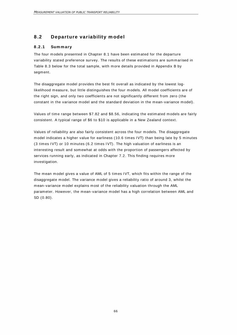
MEASUREMENT VALUATION OF PUBLIC TRANSPORT RELIABILITY
66
8.2 Departure variability model
8.2.1 Summary
The four models presented in Chapter 8.1 have been estimated for the departure
variability stated preference survey. The results of these estimations are summarised in
Table 8.3 below for the total sample, with more details provided in Appendix B by
segment.
The disaggregate model provides the best fit overall as indicated by the lowest log-
likelihood measure, but little distinguishes the four models. All model coefficients are of
the right sign, and only two coefficients are not significantly different from zero (the
constant in the variance model and the standard deviation in the mean-variance model).
Values of time range between $7.82 and $8.56, indicating the estimated models are fairly
consistent. A typical range of $6 to $10 is applicable in a New Zealand context.
Values of reliability are also fairly consistent across the four models. The disaggregate
model indicates a higher value for earliness (10.6 times IVT) than being late by 5 minutes
(3 times IVT) or 10 minutes (6.2 times IVT). The high valuation of earliness is an
interesting result and somewhat at odds with the proportion of passengers affected by
services running early, as indicated in Chapter 7.2. This finding requires more
investigation.
The mean model gives a value of AML of 5 times IVT, which fits within the range of the
disaggregate model. The variance model gives a reliability ratio of around 3, whilst the
mean-variance model explains most of the reliability valuation through the AML
parameter. However, the mean-variance model has a high correlation between AML and
SD (0.80).
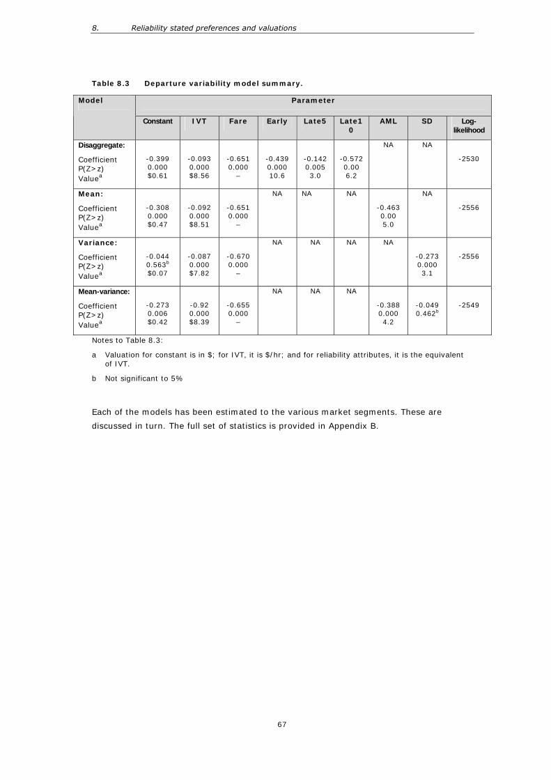
8. Reliability stated preferences and valuations
67
Table 8.3 Departure variability model summary.
Notes to Table 8.3:
a Valuation for constant is in $; for IVT, it is $/hr; and for reliability attributes, it is the equivalent of IVT.
b Not significant to 5%
Each of the models has been estimated to the various market segments. These are
discussed in turn. The full set of statistics is provided in Appendix B.
Parameter Model
Constant IVT Fare Early Late5 Late10
AML SD Log-likelihood
Disaggregate:
Coefficient P(Z>z) Valuea
-0.399 0.000 $0.61
-0.093 0.000 $8.56
-0.651 0.000
–
-0.439 0.000 10.6
-0.142 0.005 3.0
-0.572 0.00 6.2
NA NA
-2530
Mean:
Coefficient P(Z>z) Valuea
-0.308 0.000 $0.47
-0.092 0.000 $8.51
-0.651 0.000
–
NA NA NA
-0.463 0.00 5.0
NA
-2556
Variance:
Coefficient P(Z>z) Valuea
-0.044 0.563b $0.07
-0.087 0.000 $7.82
-0.670 0.000
–
NA NA NA NA
-0.273 0.000 3.1
-2556
Mean-variance:
Coefficient P(Z>z) Valuea
-0.273 0.006 $0.42
-0.92 0.000 $8.39
-0.655 0.000
–
NA NA NA
-0.388 0.000 4.2
-0.049 0.462b
-2549
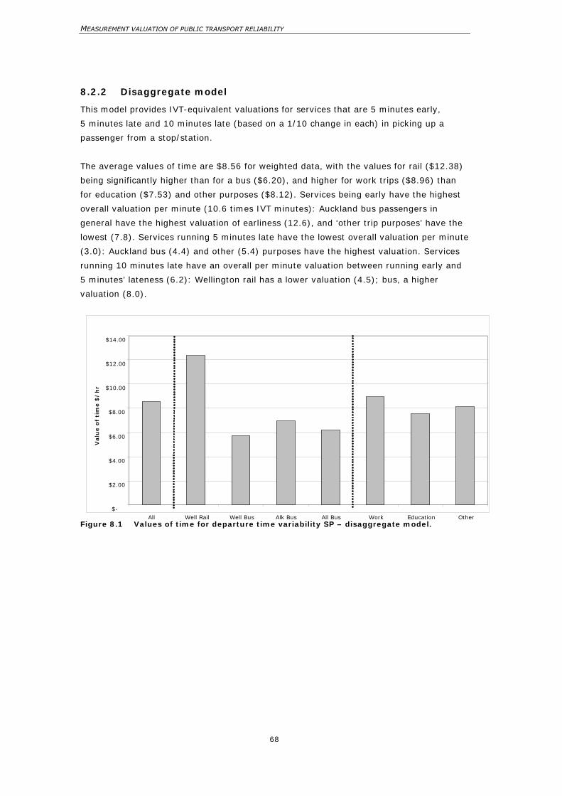
MEASUREMENT VALUATION OF PUBLIC TRANSPORT RELIABILITY
68
8.2.2 Disaggregate model
This model provides IVT-equivalent valuations for services that are 5 minutes early,
5 minutes late and 10 minutes late (based on a 1/10 change in each) in picking up a
passenger from a stop/station.
The average values of time are $8.56 for weighted data, with the values for rail ($12.38)
being significantly higher than for a bus ($6.20), and higher for work trips ($8.96) than
for education ($7.53) and other purposes ($8.12). Services being early have the highest
overall valuation per minute (10.6 times IVT minutes): Auckland bus passengers in
general have the highest valuation of earliness (12.6), and ‘other trip purposes’ have the
lowest (7.8). Services running 5 minutes late have the lowest overall valuation per minute
(3.0): Auckland bus (4.4) and other (5.4) purposes have the highest valuation. Services
running 10 minutes late have an overall per minute valuation between running early and
5 minutes’ lateness (6.2): Wellington rail has a lower valuation (4.5); bus, a higher
valuation (8.0).
Figure 8.1 Values of time for departure time variability SP – disaggregate model.
$-
$2.00
$4.00
$6.00
$8.00
$10.00
$12.00
$14.00
All Well Rail Well Bus Alk Bus All Bus Work Education Other
Valu
e o
f ti
me $
/h
r
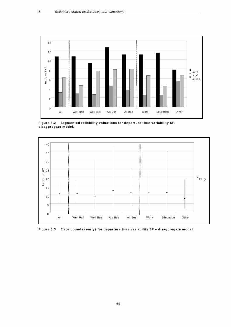
8. Reliability stated preferences and valuations
69
Figure 8.2 Segmented reliability valuations for departure time variability SP – disaggregate model.
Figure 8.3 Error bounds (early) for departure time variability SP – disaggregate model.
0
2
4
6
8
10
12
14
All Well Rail Well Bus Alk Bus All Bus Work Education Other
Rati
o t
o I
VT
Early Late5 Late10
0
5
10
15
20
25
30
35
40
All Well Rail Well Bus Alk Bus All Bus Work Education Other
Rati
o t
o I
VT
Early
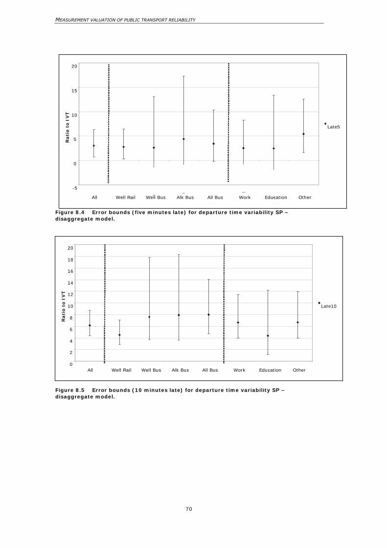
MEASUREMENT VALUATION OF PUBLIC TRANSPORT RELIABILITY
70
Figure 8.4 Error bounds (five minutes late) for departure time variability SP – disaggregate model.
Figure 8.5 Error bounds (10 minutes late) for departure time variability SP – disaggregate model.
-5
0
5
10
15
20
All Well Rail Well Bus Alk Bus All Bus Work Education Other
Rati
o t
o I
VT
Late5
0
2
4
6
8
10
12
14
16
18
20
All Well Rail Well Bus Alk Bus All Bus Work Education Other
Rati
o t
o I
VT
Late10
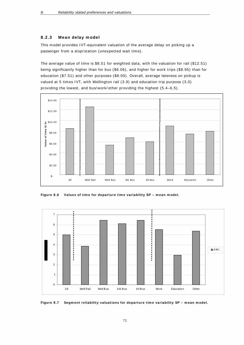
8. Reliability stated preferences and valuations
71
8.2.3 Mean delay model
This model provides IVT-equivalent valuation of the average delay on picking up a
passenger from a stop/station (unexpected wait time).
The average value of time is $8.51 for weighted data, with the valuation for rail ($12.51)
being significantly higher than for bus ($6.06), and higher for work trips ($8.95) than for
education ($7.51) and other purposes ($8.00). Overall, average lateness on pickup is
valued at 5 times IVT, with Wellington rail (3.9) and education trip purpose (3.0)
providing the lowest, and bus/work/other providing the highest (5.4–6.5).
Figure 8.6 Values of time for departure time variability SP – mean model.
Figure 8.7 Segment reliability valuations for departure time variability SP – mean model.
0
1
2
3
4
5
6
7
A ll Well Rail Well B us A lk B us A ll B us Wo rk Educatio n Other
A M L
$-
$2.00
$4.00
$6.00
$8.00
$10.00
$12.00
$14.00
All Well Rail Well Bus Alk Bus All Bus Work Education Other
Valu
e o
f ti
me $
/h
r
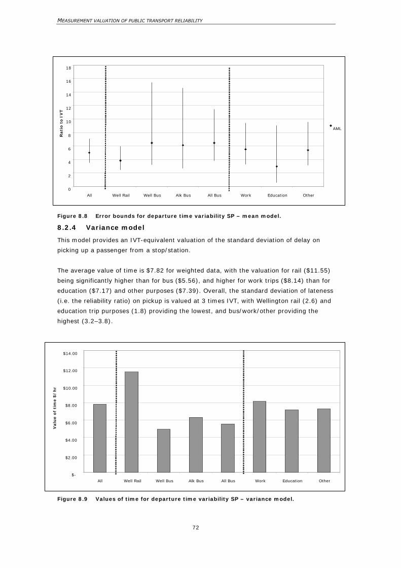
MEASUREMENT VALUATION OF PUBLIC TRANSPORT RELIABILITY
72
Figure 8.8 Error bounds for departure time variability SP – mean model.
8.2.4 Variance model
This model provides an IVT-equivalent valuation of the standard deviation of delay on
picking up a passenger from a stop/station.
The average value of time is $7.82 for weighted data, with the valuation for rail ($11.55)
being significantly higher than for bus ($5.56), and higher for work trips ($8.14) than for
education ($7.17) and other purposes ($7.39). Overall, the standard deviation of lateness
(i.e. the reliability ratio) on pickup is valued at 3 times IVT, with Wellington rail (2.6) and
education trip purposes (1.8) providing the lowest, and bus/work/other providing the
highest (3.2–3.8).
Figure 8.9 Values of time for departure time variability SP – variance model.
0
2
4
6
8
10
12
14
16
18
All Well Rail Well Bus Alk Bus All Bus Work Education Other
Rati
o t
o I
VT
AML
$-
$2.00
$4.00
$6.00
$8.00
$10.00
$12.00
$14.00
All Well Rail Well Bus Alk Bus All Bus Work Education Other
Valu
e o
f ti
me $
/h
r
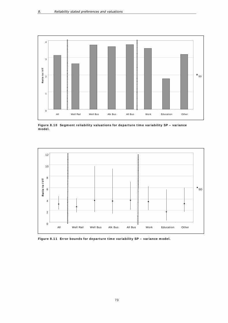
8. Reliability stated preferences and valuations
73
Figure 8.10 Segment reliability valuations for departure time variability SP – variance model.
Figure 8.11 Error bounds for departure time variability SP – variance model.
0
1
2
3
4
All Well Rail Well Bus Alk Bus All Bus Work Education Other
Rati
o t
o I
VT
SD
0
2
4
6
8
10
12
All Well Rail Well Bus Alk Bus All Bus Work Education Other
Rati
o t
o I
VT
SD
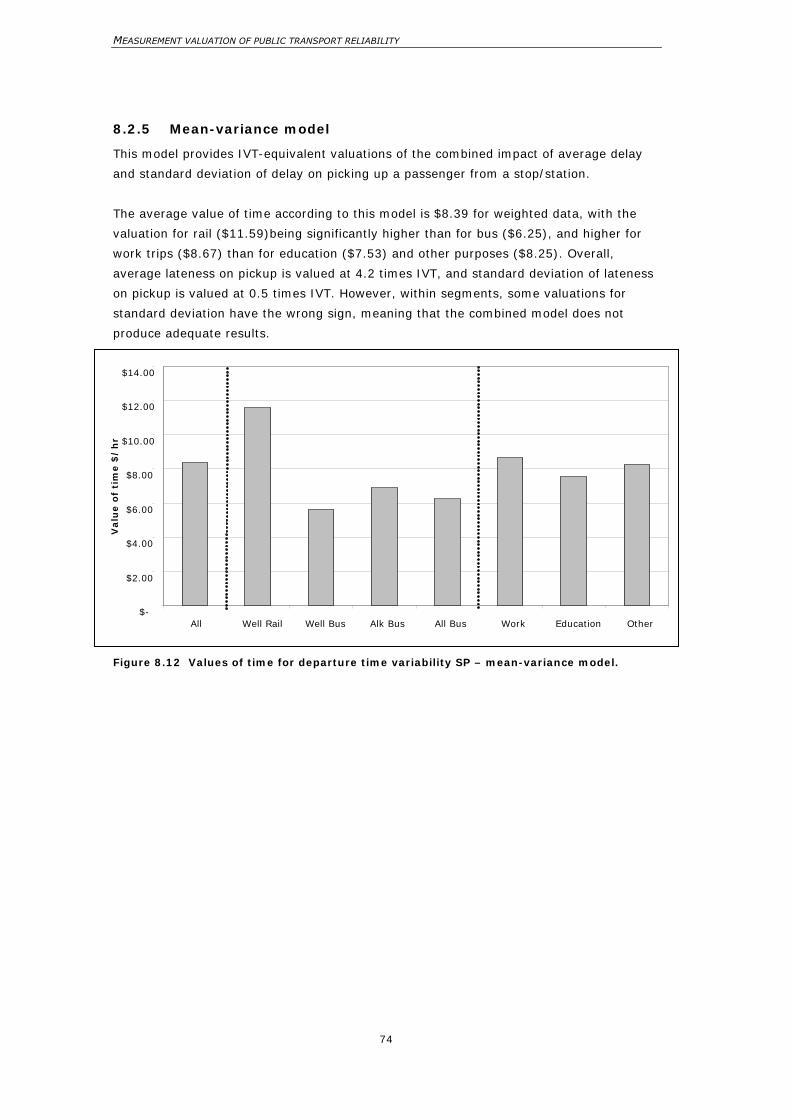
MEASUREMENT VALUATION OF PUBLIC TRANSPORT RELIABILITY
74
8.2.5 Mean-variance model
This model provides IVT-equivalent valuations of the combined impact of average delay
and standard deviation of delay on picking up a passenger from a stop/station.
The average value of time according to this model is $8.39 for weighted data, with the
valuation for rail ($11.59)being significantly higher than for bus ($6.25), and higher for
work trips ($8.67) than for education ($7.53) and other purposes ($8.25). Overall,
average lateness on pickup is valued at 4.2 times IVT, and standard deviation of lateness
on pickup is valued at 0.5 times IVT. However, within segments, some valuations for
standard deviation have the wrong sign, meaning that the combined model does not
produce adequate results.
Figure 8.12 Values of time for departure time variability SP – mean-variance model.
$-
$2.00
$4.00
$6.00
$8.00
$10.00
$12.00
$14.00
All Well Rail Well Bus Alk Bus All Bus Work Education Other
Valu
e o
f ti
me $
/h
r
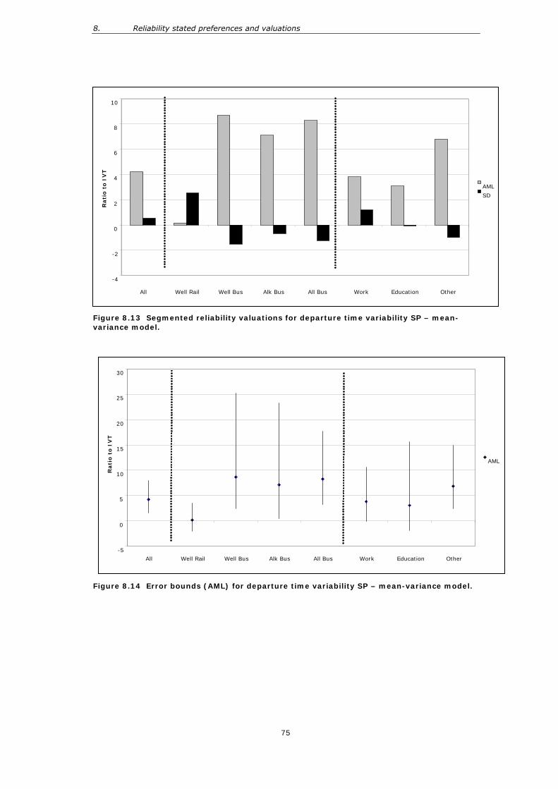
8. Reliability stated preferences and valuations
75
Figure 8.13 Segmented reliability valuations for departure time variability SP – mean-variance model.
Figure 8.14 Error bounds (AML) for departure time variability SP – mean-variance model.
-4
-2
0
2
4
6
8
10
All Well Rail Well Bus Alk Bus All Bus Work Education Other
Rati
o t
o I
VT
AML
SD
-5
0
5
10
15
20
25
30
All Well Rail Well Bus Alk Bus All Bus Work Education Other
Rati
o t
o I
VT
AML
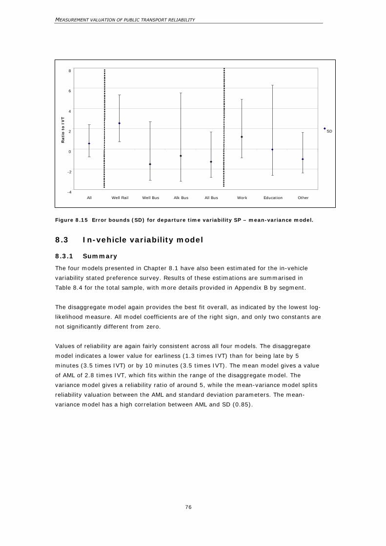
MEASUREMENT VALUATION OF PUBLIC TRANSPORT RELIABILITY
76
Figure 8.15 Error bounds (SD) for departure time variability SP – mean-variance model.
8.3 In-vehicle variability model
8.3.1 Summary
The four models presented in Chapter 8.1 have also been estimated for the in-vehicle
variability stated preference survey. Results of these estimations are summarised in
Table 8.4 for the total sample, with more details provided in Appendix B by segment.
The disaggregate model again provides the best fit overall, as indicated by the lowest log-
likelihood measure. All model coefficients are of the right sign, and only two constants are
not significantly different from zero.
Values of reliability are again fairly consistent across all four models. The disaggregate
model indicates a lower value for earliness (1.3 times IVT) than for being late by 5
minutes (3.5 times IVT) or by 10 minutes (3.5 times IVT). The mean model gives a value
of AML of 2.8 times IVT, which fits within the range of the disaggregate model. The
variance model gives a reliability ratio of around 5, while the mean-variance model splits
reliability valuation between the AML and standard deviation parameters. The mean-
variance model has a high correlation between AML and SD (0.85).
-4
-2
0
2
4
6
8
All Well Rail Well Bus Alk Bus All Bus Work Education Other
Rati
o t
o I
VT
SD
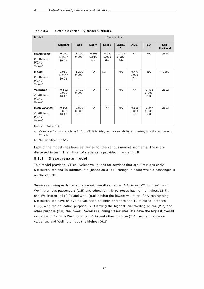
8. Reliability stated preferences and valuations
77
Table 8.4 In-vehicle variability model summary.
Notes to Table 8.4:
a Valuation for constant is in $; for IVT, it is $/hr; and for reliability attributes, it is the equivalent of IVT.
b Not significant to 5%
Each of the models has been estimated for the various market segments. These are
discussed in turn. The full set of statistics is provided in Appendix B.
8.3.2 Disaggregate model
This model provides IVT-equivalent valuations for services that are 5 minutes early,
5 minutes late and 10 minutes late (based on a 1/10 change in each) while a passenger is
on the vehicle.
Services running early have the lowest overall valuation (1.3 times IVT minutes), with
Wellington bus passengers (2.5) and education trip purposes having the highest (2.7),
and Wellington rail (0.3) and work (0.8) having the lowest valuation. Services running
5 minutes late have an overall valuation between earliness and 10 minutes’ lateness
(3.5), with the education purpose (5.7) having the highest, and Wellington rail (2.7) and
other purpose (2.8) the lowest. Services running 10 minutes late have the highest overall
valuation (4.5), with Wellington rail (3.9) and other purpose (3.4) having the lowest
valuation, and Wellington bus the highest (6.2)
Parameter Model
Constant Fare Early Late5 Late10
AML SD Log-likelihood
Disaggregate:
Coefficient P(Z>z) Valuea
-0.051 0.154b $0.05
-1.120 0.000
-0.103 0.016 1.3
-0.282 0.000 3.5
-0.719 0.000 4.5
NA NA -2544
Mean:
Coefficient P(Z>z) Valuea
0.012 0.735b
$0.01
-1.220 0.000
–
NA NA NA -0.477 0.000 2.8
NA --2583
Variance:
Coefficient P(Z>z) Valuea
-0.132 0.000 $0.19
-0.702 0.000
–
NA NA NA NA -0.483 0.000 5.3
-2592
Mean-variance:
Coefficient P(Z>z) Valuea
-0.105 0.003 $0.12
-0.888 0.000
–
NA NA NA -0.158 0.000 1.3
-0.347 0.000 2.8
-2583
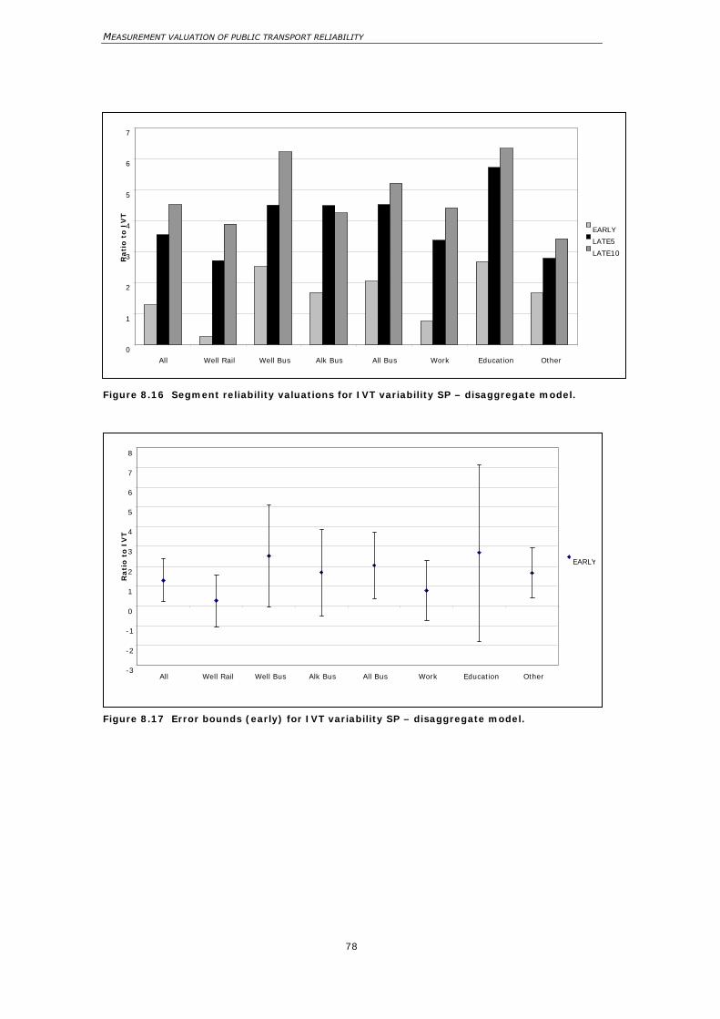
MEASUREMENT VALUATION OF PUBLIC TRANSPORT RELIABILITY
78
Figure 8.16 Segment reliability valuations for IVT variability SP – disaggregate model.
Figure 8.17 Error bounds (early) for IVT variability SP – disaggregate model.
-3
-2
-1
0 1 2 3 4 5 6 7 8
All Well Rail Well Bus Alk Bus All Bus Work Education Other
Rati
o t
o I
VT
EARLY
0
1
2
3
4
5
6
7
All Well Rail Well Bus Alk Bus All Bus Work Education Other
Rati
o t
o I
VT
EARLY
LATE5
LATE10
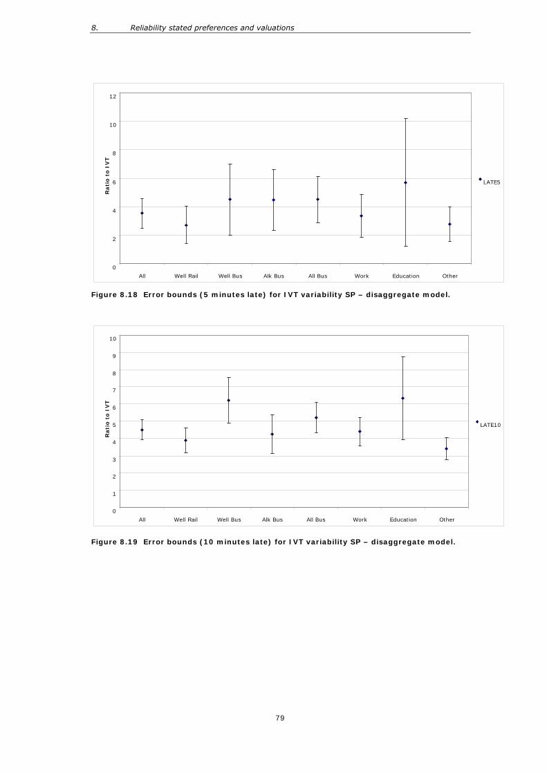
8. Reliability stated preferences and valuations
79
Figure 8.18 Error bounds (5 minutes late) for IVT variability SP – disaggregate model.
Figure 8.19 Error bounds (10 minutes late) for IVT variability SP – disaggregate model.
0
1
2
3
4
5
6
7
8
9
10
All Well Rail Well Bus Alk Bus All Bus Work Education Other
Rati
o t
o I
VT
LATE10
0
2
4
6
8
10
12
All Well Rail Well Bus Alk Bus All Bus Work Education Other
Rati
o t
o I
VT
LATE5
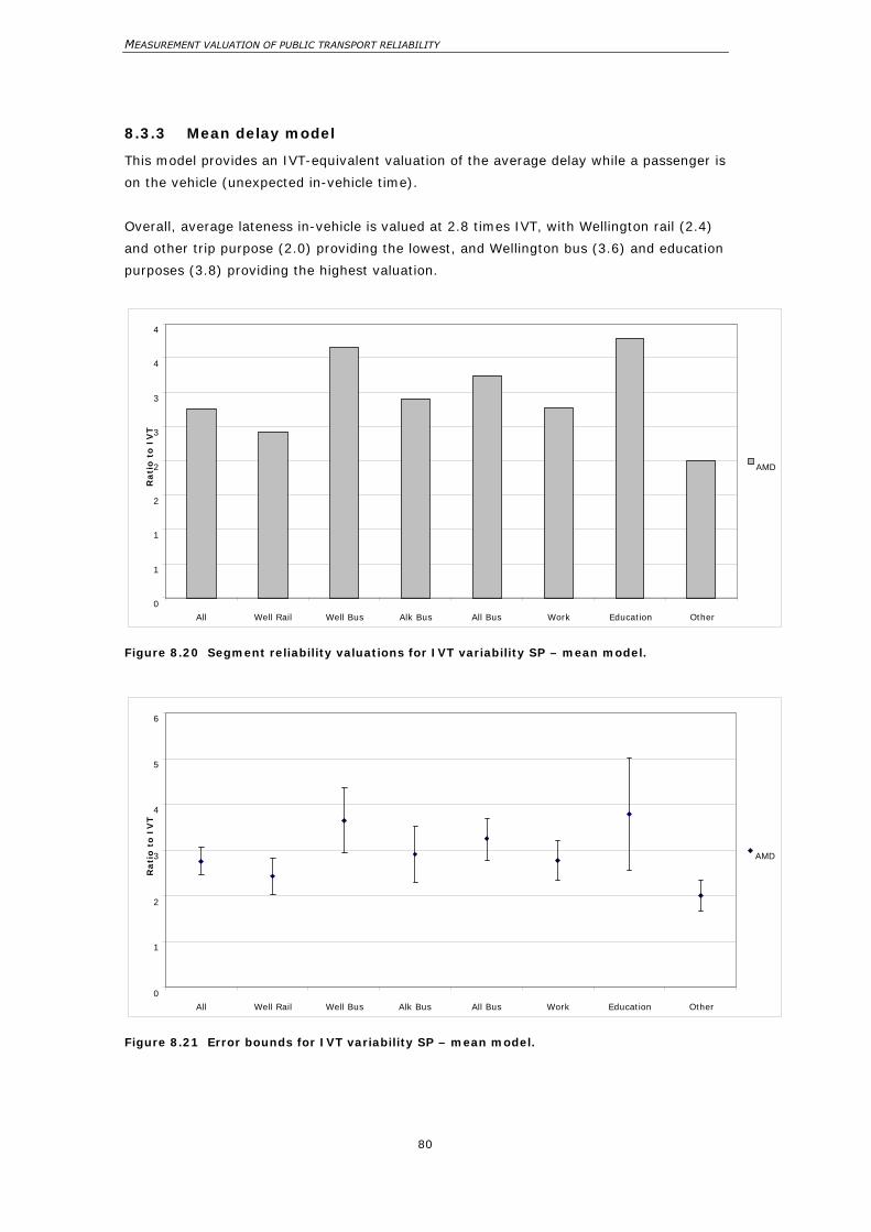
MEASUREMENT VALUATION OF PUBLIC TRANSPORT RELIABILITY
80
8.3.3 Mean delay model
This model provides an IVT-equivalent valuation of the average delay while a passenger is
on the vehicle (unexpected in-vehicle time).
Overall, average lateness in-vehicle is valued at 2.8 times IVT, with Wellington rail (2.4)
and other trip purpose (2.0) providing the lowest, and Wellington bus (3.6) and education
purposes (3.8) providing the highest valuation.
Figure 8.20 Segment reliability valuations for IVT variability SP – mean model.
Figure 8.21 Error bounds for IVT variability SP – mean model.
0
1
2
3
4
5
6
All Well Rail Well Bus Alk Bus All Bus Work Education Other
Rati
o t
o I
VT
AMD
0
1
1
2
2
3
3
4
4
All Well Rail Well Bus Alk Bus All Bus Work Education Other
Rati
o t
o I
VT
AMD
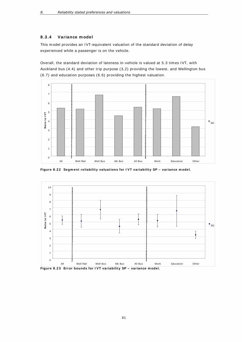
8. Reliability stated preferences and valuations
81
8.3.4 Variance model
This model provides an IVT-equivalent valuation of the standard deviation of delay
experienced while a passenger is on the vehicle.
Overall, the standard deviation of lateness in-vehicle is valued at 5.3 times IVT, with
Auckland bus (4.4) and other trip purpose (3,2) providing the lowest, and Wellington bus
(6.7) and education purposes (6.6) providing the highest valuation.
Figure 8.22 Segment reliability valuations for IVT variability SP – variance model.
Figure 8.23 Error bounds for IVT variability SP – variance model.
0
1
2
3
4
5
6
7
8
All Well Rail Well Bus Alk Bus All Bus Work Education Other
Rati
o t
o I
VT
SD
0
1
2
3
4
5
6
7
8
9
10
All Well Rail Well Bus Alk Bus All Bus Work Education Other
Rati
o t
o I
VT
SD
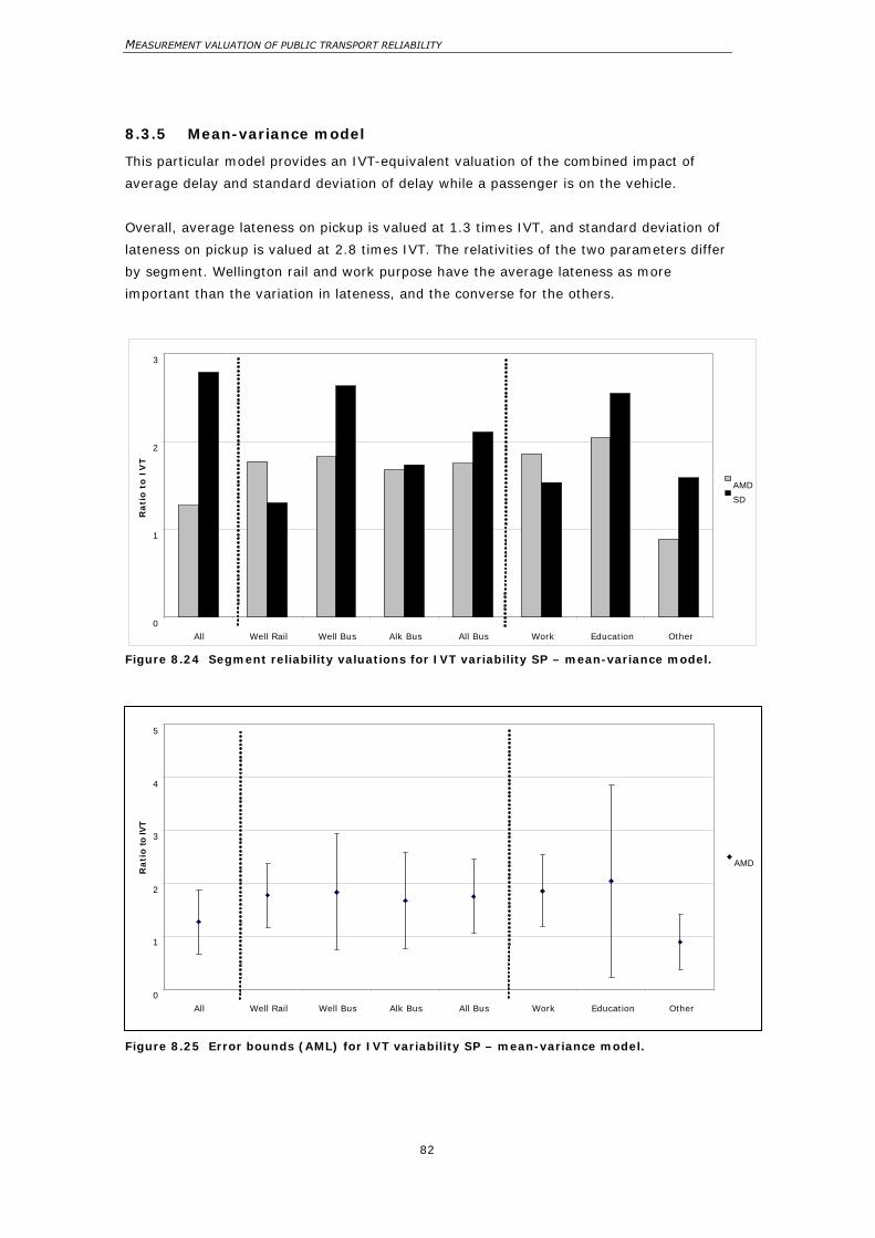
MEASUREMENT VALUATION OF PUBLIC TRANSPORT RELIABILITY
82
8.3.5 Mean-variance model
This particular model provides an IVT-equivalent valuation of the combined impact of
average delay and standard deviation of delay while a passenger is on the vehicle.
Overall, average lateness on pickup is valued at 1.3 times IVT, and standard deviation of
lateness on pickup is valued at 2.8 times IVT. The relativities of the two parameters differ
by segment. Wellington rail and work purpose have the average lateness as more
important than the variation in lateness, and the converse for the others.
Figure 8.24 Segment reliability valuations for IVT variability SP – mean-variance model.
Figure 8.25 Error bounds (AML) for IVT variability SP – mean-variance model.
0
1
2
3
All Well Rail Well Bus Alk Bus All Bus Work Education Other
Rati
o t
o I
VT
AMD SD
0
1
2
3
4
5
All Well Rail Well Bus Alk Bus All Bus Work Education Other
Rati
o to
IVT
AMD
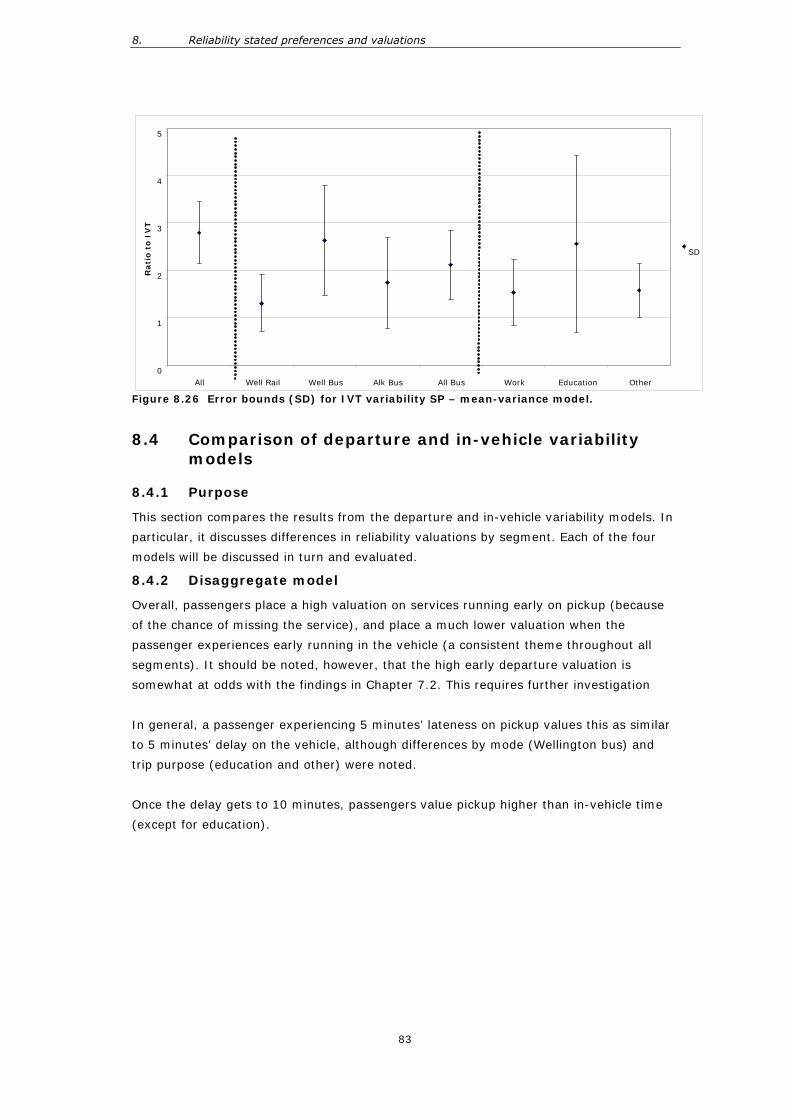
8. Reliability stated preferences and valuations
83
Figure 8.26 Error bounds (SD) for IVT variability SP – mean-variance model.
8.4 Comparison of departure and in-vehicle variability models
8.4.1 Purpose
This section compares the results from the departure and in-vehicle variability models. In
particular, it discusses differences in reliability valuations by segment. Each of the four
models will be discussed in turn and evaluated.
8.4.2 Disaggregate model
Overall, passengers place a high valuation on services running early on pickup (because
of the chance of missing the service), and place a much lower valuation when the
passenger experiences early running in the vehicle (a consistent theme throughout all
segments). It should be noted, however, that the high early departure valuation is
somewhat at odds with the findings in Chapter 7.2. This requires further investigation
In general, a passenger experiencing 5 minutes’ lateness on pickup values this as similar
to 5 minutes’ delay on the vehicle, although differences by mode (Wellington bus) and
trip purpose (education and other) were noted.
Once the delay gets to 10 minutes, passengers value pickup higher than in-vehicle time
(except for education).
0
1
2
3
4
5
All Well Rail Well Bus Alk Bus All Bus Work Education Other
Rati
o t
o I
VT
SD
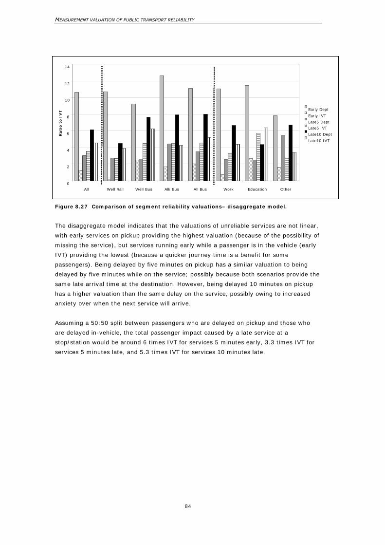
MEASUREMENT VALUATION OF PUBLIC TRANSPORT RELIABILITY
84
Figure 8.27 Comparison of segment reliability valuations– disaggregate model.
The disaggregate model indicates that the valuations of unreliable services are not linear,
with early services on pickup providing the highest valuation (because of the possibility of
missing the service), but services running early while a passenger is in the vehicle (early
IVT) providing the lowest (because a quicker journey time is a benefit for some
passengers). Being delayed by five minutes on pickup has a similar valuation to being
delayed by five minutes while on the service; possibly because both scenarios provide the
same late arrival time at the destination. However, being delayed 10 minutes on pickup
has a higher valuation than the same delay on the service, possibly owing to increased
anxiety over when the next service will arrive.
Assuming a 50:50 split between passengers who are delayed on pickup and those who
are delayed in-vehicle, the total passenger impact caused by a late service at a
stop/station would be around 6 times IVT for services 5 minutes early, 3.3 times IVT for
services 5 minutes late, and 5.3 times IVT for services 10 minutes late.
0
2
4
6
8
10
12
14
All Well Rail Well Bus Alk Bus All Bus Work Education Other
Rati
o t
o I
VT Early Dept
Early IVT Late5 Dept Late5 IVT
Late10 Dept
Late10 IVT
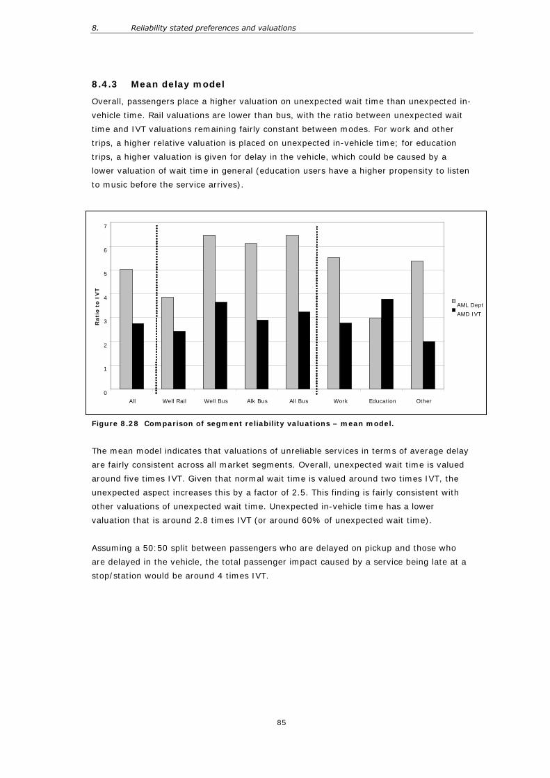
8. Reliability stated preferences and valuations
85
8.4.3 Mean delay model
Overall, passengers place a higher valuation on unexpected wait time than unexpected in-
vehicle time. Rail valuations are lower than bus, with the ratio between unexpected wait
time and IVT valuations remaining fairly constant between modes. For work and other
trips, a higher relative valuation is placed on unexpected in-vehicle time; for education
trips, a higher valuation is given for delay in the vehicle, which could be caused by a
lower valuation of wait time in general (education users have a higher propensity to listen
to music before the service arrives).
Figure 8.28 Comparison of segment reliability valuations – mean model.
The mean model indicates that valuations of unreliable services in terms of average delay
are fairly consistent across all market segments. Overall, unexpected wait time is valued
around five times IVT. Given that normal wait time is valued around two times IVT, the
unexpected aspect increases this by a factor of 2.5. This finding is fairly consistent with
other valuations of unexpected wait time. Unexpected in-vehicle time has a lower
valuation that is around 2.8 times IVT (or around 60% of unexpected wait time).
Assuming a 50:50 split between passengers who are delayed on pickup and those who
are delayed in the vehicle, the total passenger impact caused by a service being late at a
stop/station would be around 4 times IVT.
0
1
2
3
4
5
6
7
All Well Rail Well Bus Alk Bus All Bus Work Education Other
Rati
o t
o I
VT
AML Dept AMD IVT
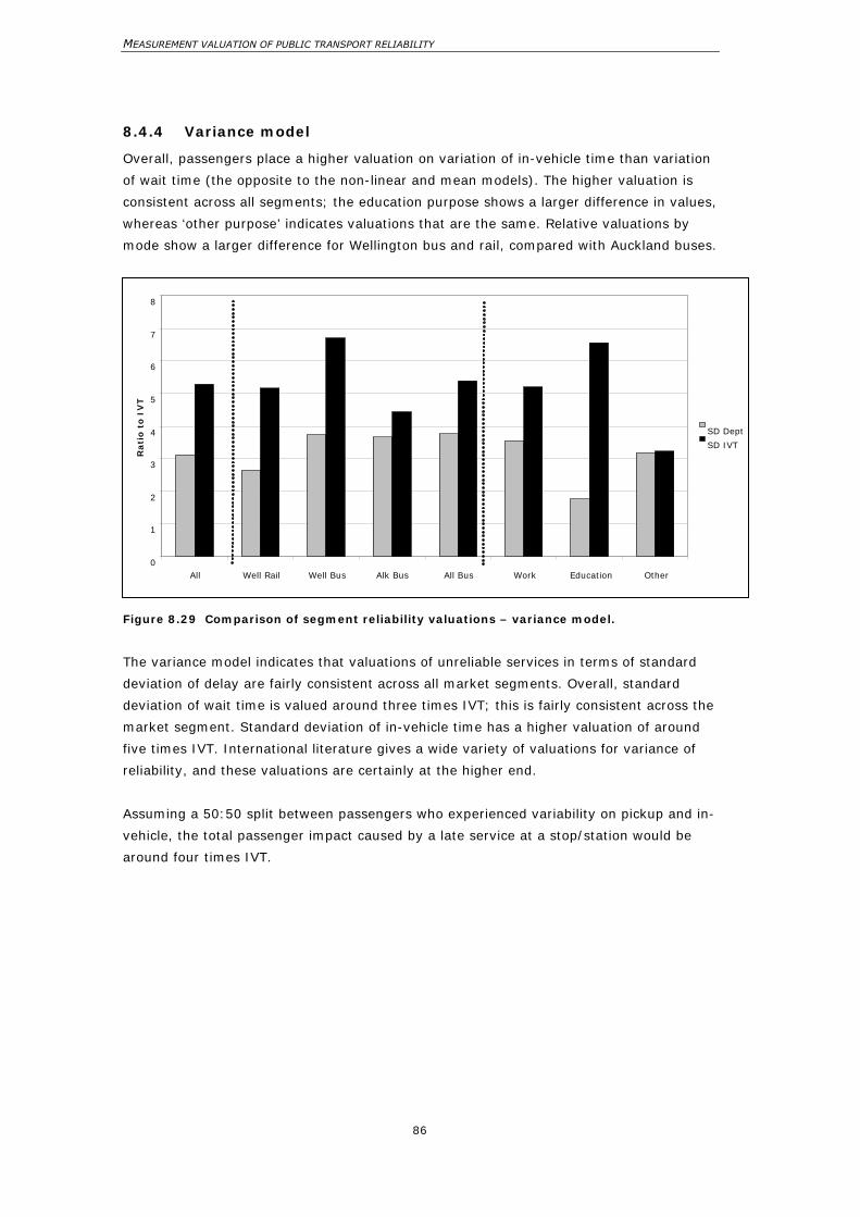
MEASUREMENT VALUATION OF PUBLIC TRANSPORT RELIABILITY
86
8.4.4 Variance model
Overall, passengers place a higher valuation on variation of in-vehicle time than variation
of wait time (the opposite to the non-linear and mean models). The higher valuation is
consistent across all segments; the education purpose shows a larger difference in values,
whereas ‘other purpose’ indicates valuations that are the same. Relative valuations by
mode show a larger difference for Wellington bus and rail, compared with Auckland buses.
Figure 8.29 Comparison of segment reliability valuations – variance model.
The variance model indicates that valuations of unreliable services in terms of standard
deviation of delay are fairly consistent across all market segments. Overall, standard
deviation of wait time is valued around three times IVT; this is fairly consistent across the
market segment. Standard deviation of in-vehicle time has a higher valuation of around
five times IVT. International literature gives a wide variety of valuations for variance of
reliability, and these valuations are certainly at the higher end.
Assuming a 50:50 split between passengers who experienced variability on pickup and in-
vehicle, the total passenger impact caused by a late service at a stop/station would be
around four times IVT.
0
1
2
3
4
5
6
7
8
All Well Rail Well Bus Alk Bus All Bus Work Education Other
Rati
o t
o I
VT
SD Dept SD IVT
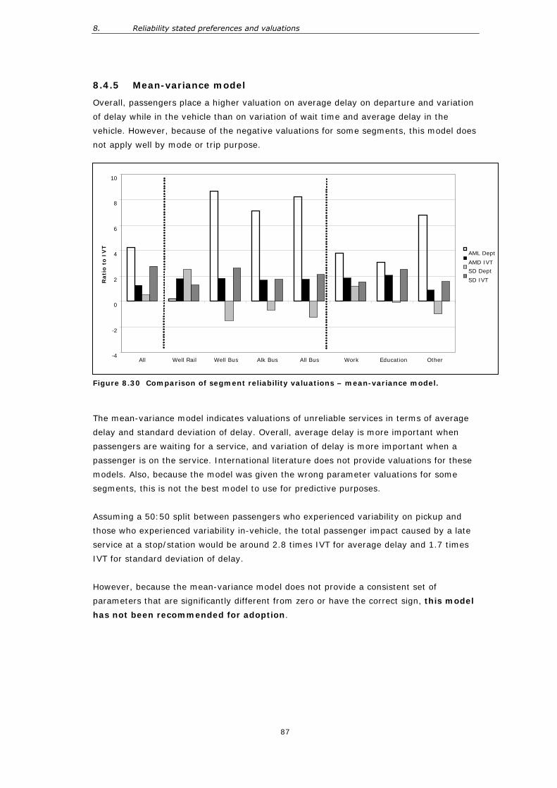
8. Reliability stated preferences and valuations
87
8.4.5 Mean-variance model
Overall, passengers place a higher valuation on average delay on departure and variation
of delay while in the vehicle than on variation of wait time and average delay in the
vehicle. However, because of the negative valuations for some segments, this model does
not apply well by mode or trip purpose.
Figure 8.30 Comparison of segment reliability valuations – mean-variance model.
The mean-variance model indicates valuations of unreliable services in terms of average
delay and standard deviation of delay. Overall, average delay is more important when
passengers are waiting for a service, and variation of delay is more important when a
passenger is on the service. International literature does not provide valuations for these
models. Also, because the model was given the wrong parameter valuations for some
segments, this is not the best model to use for predictive purposes.
Assuming a 50:50 split between passengers who experienced variability on pickup and
those who experienced variability in-vehicle, the total passenger impact caused by a late
service at a stop/station would be around 2.8 times IVT for average delay and 1.7 times
IVT for standard deviation of delay.
However, because the mean-variance model does not provide a consistent set of
parameters that are significantly different from zero or have the correct sign, this model
has not been recommended for adoption.
-4
-2
0
2
4
6
8
10
All Well Rail Well Bus Alk Bus All Bus Work Education Other
Rati
o t
o I
VT
AML Dept AMD IVT SD Dept SD IVT
MEASUREMENT VALUATION OF PUBLIC TRANSPORT RELIABILITY
88
8.5 Implications for planning – recommended valuations
8.5.1 Summary
A summary of the valuations from the SP is provided in Table 8.5. This study was able to
separate departure and in-vehicle reliability; in the real world, however, the impact on an
individual service will be a combination of the two sources of delay. A service that is
running five minutes late will result in the passengers still to be picked up being late on
departure, and the passengers already on the service being delayed in-vehicle by five
minutes. By knowing where the delay occurs on the route, the proportion of passengers
affected by both delays can be determined, and so a weighted average impact can be
calculated. Without this information, you could roughly assume a 50:50 split between the
two effects (the combined column).
Depending on the information that is available to practitioners, any of the models and
parameters listed in Table 8.5 could be used. However, it should be recognised that
applying the different models to the same dataset (albeit with different indicators) will
produce different demand impacts (see examples 1–3 in Chapter 9). In particular, a
scenario that currently has some early or very late running services will show a bigger
uplift when using the disaggregate or variance approach. Where levels of reliability are
lower, the difference between the three approaches is smaller.
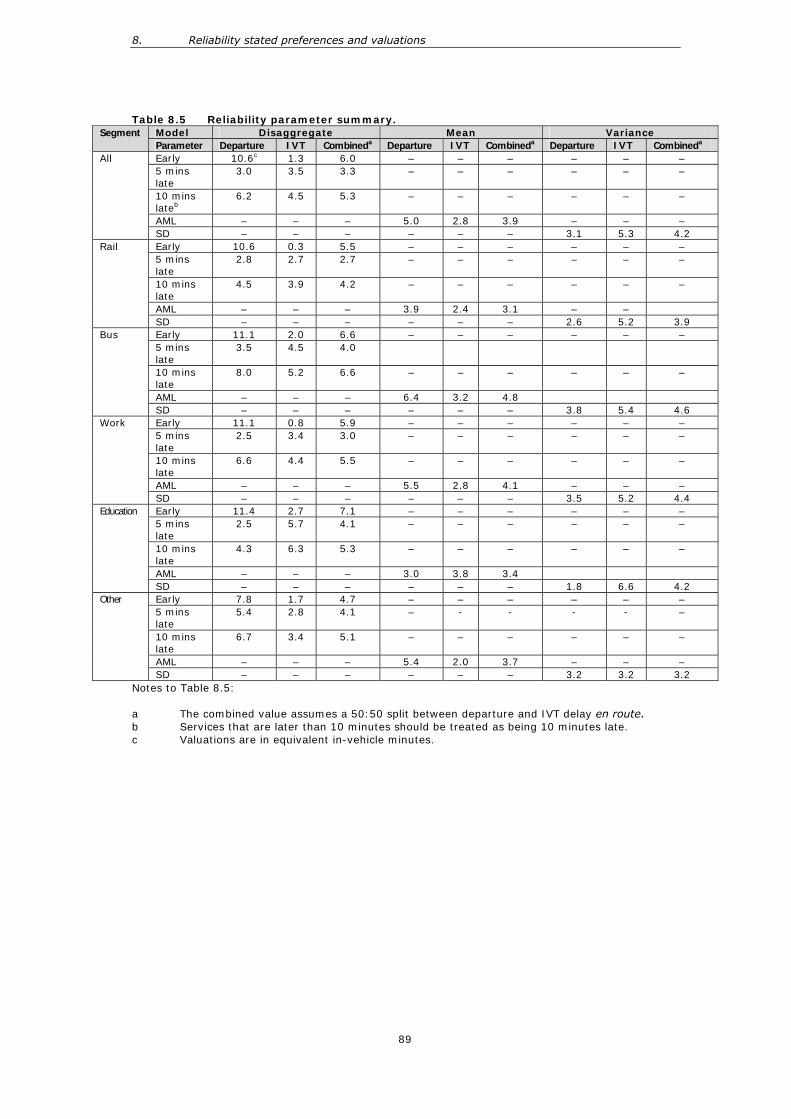
8. Reliability stated preferences and valuations
89
Table 8.5 Reliability parameter summary. Model Disaggregate Mean Variance Segment Parameter Departure IVT Combineda Departure IVT Combineda Departure IVT Combineda Early 10.6c 1.3 6.0 – – – – – – 5 mins late
3.0 3.5 3.3 – – – – – –
10 mins lateb
6.2 4.5 5.3 – – – – – –
AML – – – 5.0 2.8 3.9 – – –
All
SD – – – – – – 3.1 5.3 4.2 Early 10.6 0.3 5.5 – – – – – – 5 mins late
2.8 2.7 2.7 – – – – – –
10 mins late
4.5 3.9 4.2 – – – – – –
AML – – – 3.9 2.4 3.1 – –
Rail
SD – – – – – – 2.6 5.2 3.9 Early 11.1 2.0 6.6 – – – – – – 5 mins late
3.5 4.5 4.0
10 mins late
8.0 5.2 6.6 – – – – – –
AML – – – 6.4 3.2 4.8
Bus
SD – – – – – – 3.8 5.4 4.6 Early 11.1 0.8 5.9 – – – – – – 5 mins late
2.5 3.4 3.0 – – – – – –
10 mins late
6.6 4.4 5.5 – – – – – –
AML – – – 5.5 2.8 4.1 – – –
Work
SD – – – – – – 3.5 5.2 4.4 Early 11.4 2.7 7.1 – – – – – – 5 mins late
2.5 5.7 4.1 – – – – – –
10 mins late
4.3 6.3 5.3 – – – – – –
AML – – – 3.0 3.8 3.4
Education
SD – – – – – – 1.8 6.6 4.2 Early 7.8 1.7 4.7 – – – – – – 5 mins late
5.4 2.8 4.1 – - - - - –
10 mins late
6.7 3.4 5.1 – – – – – –
AML – – – 5.4 2.0 3.7 – – –
Other
SD – – – – – – 3.2 3.2 3.2 Notes to Table 8.5: a The combined value assumes a 50:50 split between departure and IVT delay en route. b Services that are later than 10 minutes should be treated as being 10 minutes late. c Valuations are in equivalent in-vehicle minutes.
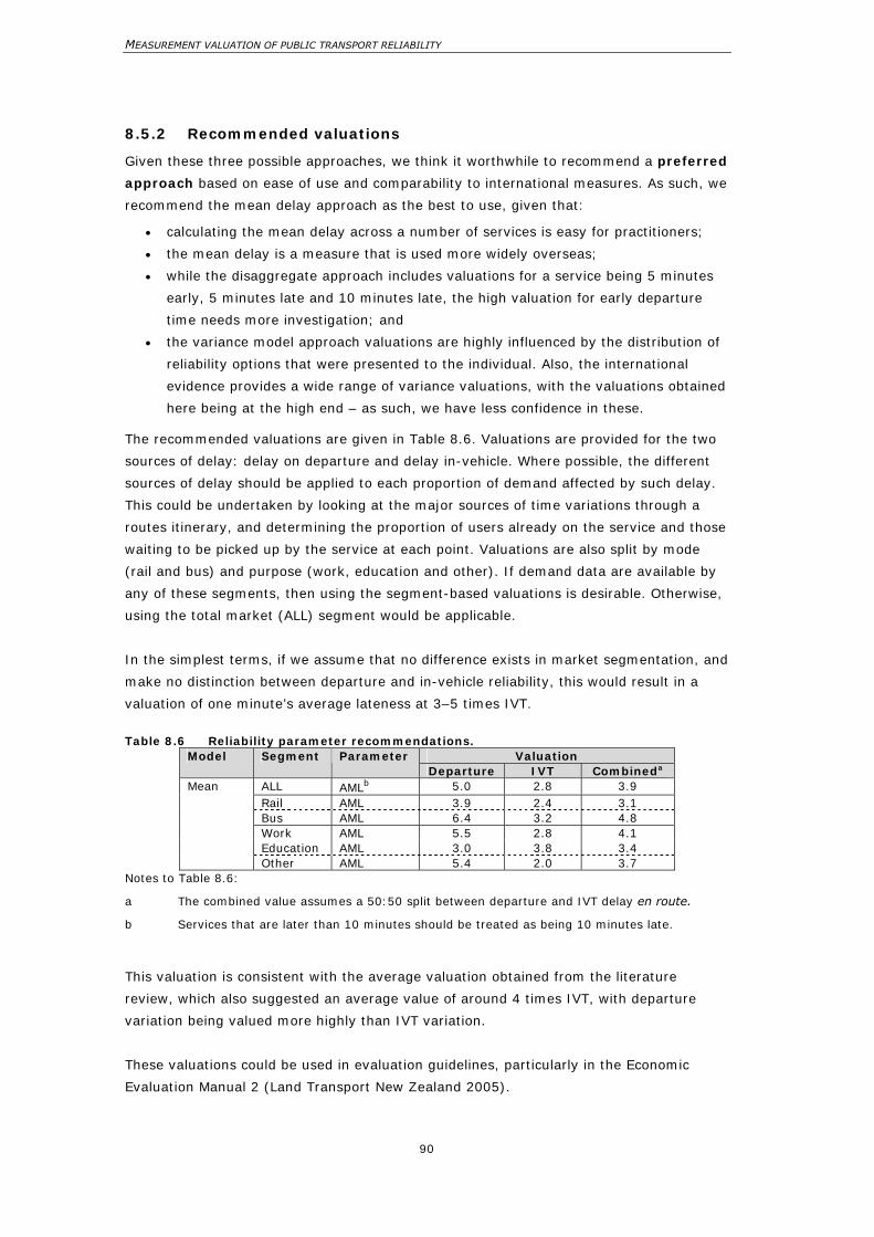
MEASUREMENT VALUATION OF PUBLIC TRANSPORT RELIABILITY
90
8.5.2 Recommended valuations
Given these three possible approaches, we think it worthwhile to recommend a preferred
approach based on ease of use and comparability to international measures. As such, we
recommend the mean delay approach as the best to use, given that:
• calculating the mean delay across a number of services is easy for practitioners;
• the mean delay is a measure that is used more widely overseas;
• while the disaggregate approach includes valuations for a service being 5 minutes
early, 5 minutes late and 10 minutes late, the high valuation for early departure
time needs more investigation; and
• the variance model approach valuations are highly influenced by the distribution of
reliability options that were presented to the individual. Also, the international
evidence provides a wide range of variance valuations, with the valuations obtained
here being at the high end – as such, we have less confidence in these.
The recommended valuations are given in Table 8.6. Valuations are provided for the two
sources of delay: delay on departure and delay in-vehicle. Where possible, the different
sources of delay should be applied to each proportion of demand affected by such delay.
This could be undertaken by looking at the major sources of time variations through a
routes itinerary, and determining the proportion of users already on the service and those
waiting to be picked up by the service at each point. Valuations are also split by mode
(rail and bus) and purpose (work, education and other). If demand data are available by
any of these segments, then using the segment-based valuations is desirable. Otherwise,
using the total market (ALL) segment would be applicable.
In the simplest terms, if we assume that no difference exists in market segmentation, and
make no distinction between departure and in-vehicle reliability, this would result in a
valuation of one minute’s average lateness at 3–5 times IVT.
Table 8.6 Reliability parameter recommendations.
Valuation Model Segment Parameter Departure IVT Combineda
ALL AMLb 5.0 2.8 3.9 Rail AML 3.9 2.4 3.1 Bus AML 6.4 3.2 4.8 Work AML 5.5 2.8 4.1 Education AML 3.0 3.8 3.4
Mean
Other AML 5.4 2.0 3.7 Notes to Table 8.6:
a The combined value assumes a 50:50 split between departure and IVT delay en route.
b Services that are later than 10 minutes should be treated as being 10 minutes late.
This valuation is consistent with the average valuation obtained from the literature
review, which also suggested an average value of around 4 times IVT, with departure
variation being valued more highly than IVT variation.
These valuations could be used in evaluation guidelines, particularly in the Economic
Evaluation Manual 2 (Land Transport New Zealand 2005).
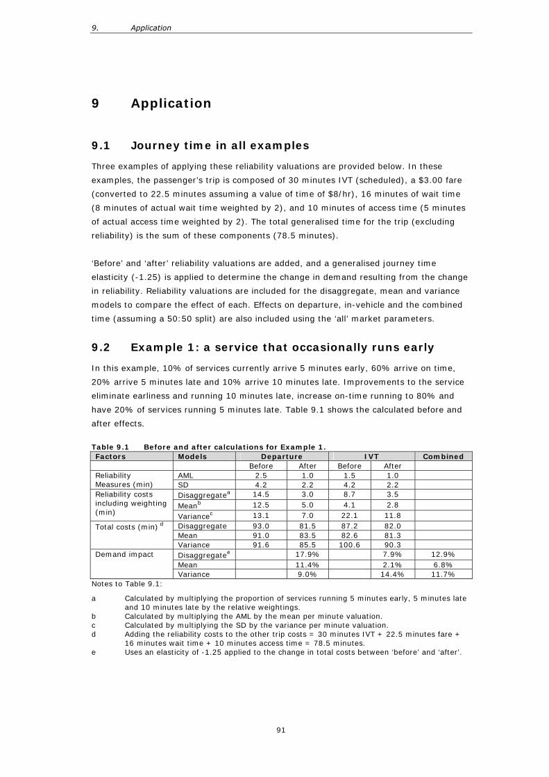
9. Application
91
9 Application
9.1 Journey time in all examples
Three examples of applying these reliability valuations are provided below. In these
examples, the passenger’s trip is composed of 30 minutes IVT (scheduled), a $3.00 fare
(converted to 22.5 minutes assuming a value of time of $8/hr), 16 minutes of wait time
(8 minutes of actual wait time weighted by 2), and 10 minutes of access time (5 minutes
of actual access time weighted by 2). The total generalised time for the trip (excluding
reliability) is the sum of these components (78.5 minutes).
‘Before’ and ‘after’ reliability valuations are added, and a generalised journey time
elasticity (-1.25) is applied to determine the change in demand resulting from the change
in reliability. Reliability valuations are included for the disaggregate, mean and variance
models to compare the effect of each. Effects on departure, in-vehicle and the combined
time (assuming a 50:50 split) are also included using the ‘all’ market parameters.
9.2 Example 1: a service that occasionally runs early
In this example, 10% of services currently arrive 5 minutes early, 60% arrive on time,
20% arrive 5 minutes late and 10% arrive 10 minutes late. Improvements to the service
eliminate earliness and running 10 minutes late, increase on-time running to 80% and
have 20% of services running 5 minutes late. Table 9.1 shows the calculated before and
after effects.
Table 9.1 Before and after calculations for Example 1. Factors Models Departure IVT Combined Before After Before After
AML 2.5 1.0 1.5 1.0 Reliability Measures (min) SD 4.2 2.2 4.2 2.2
Disaggregatea 14.5 3.0 8.7 3.5
Meanb 12.5 5.0 4.1 2.8 Reliability costs including weighting (min) Variancec 13.1 7.0 22.1 11.8
Disaggregate 93.0 81.5 87.2 82.0 Mean 91.0 83.5 82.6 81.3
Total costs (min) d
Variance 91.6 85.5 100.6 90.3 Disaggregatee 17.9% 7.9% 12.9% Mean 11.4% 2.1% 6.8%
Demand impact
Variance 9.0% 14.4% 11.7% Notes to Table 9.1:
a Calculated by multiplying the proportion of services running 5 minutes early, 5 minutes late and 10 minutes late by the relative weightings.
b Calculated by multiplying the AML by the mean per minute valuation. c Calculated by multiplying the SD by the variance per minute valuation. d Adding the reliability costs to the other trip costs = 30 minutes IVT + 22.5 minutes fare +
16 minutes wait time + 10 minutes access time = 78.5 minutes. e Uses an elasticity of -1.25 applied to the change in total costs between ‘before’ and ‘after’.
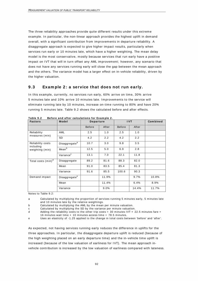
MEASUREMENT VALUATION OF PUBLIC TRANSPORT RELIABILITY
92
The three reliability approaches provide quite different results under this extreme
example. In particular, the non-linear approach provides the highest uplift in demand
overall, with a significant contribution from improvements in departure reliability. A
disaggregate approach is expected to give higher impact results, particularly when
services run early or 10 minutes late, which have a higher weighting. The mean delay
model is the most conservative, mostly because services that run early have a positive
impact on IVT that will in turn offset any AML improvement; however, any scenario that
does not have any services running early will close the gap between the mean approach
and the others. The variance model has a larger effect on in-vehicle reliability, driven by
the higher valuation.
9.3 Example 2: a service that does not run early.
In this example, currently, no services run early, 60% arrive on time, 30% arrive
5 minutes late and 10% arrive 10 minutes late. Improvements to the service will
eliminate running late by 10 minutes, increase on-time running to 80% and have 20%
running 5 minutes late. Table 9.2 shows the calculated before and after effects.
Table 9.2 Before and after calculations for Example 2. Factors Model Departure IVT Combined
Before After Before After
AML 2.5 1.0 2.5 1.0 Reliability measures (min)
SD 4.2 2.2 4.2 2.2
Disaggregatea 10.7 3.0 9.8 3.5
Meanb 12.5 5.0 6.9 2.8
Reliability costs including weighting (min)
Variancec 13.1 7.0 22.1 11.8
Disaggregate 89.2 81.6 88.3 82.0
Mean 91.0 83.5 85.4 81.3
Total costs (min)d
Variance 91.6 85.5 100.6 90.3
Disaggregatee 11.9% 9.7% 10.8%
Mean 11.4% 6.4% 8.9%
Demand impact
Variance 9.0% 14.4% 11.7%
Notes to Table 9.2:
a Calculated by multiplying the proportion of services running 5 minutes early, 5 minutes late and 10 minutes late by the relative weightings.
b Calculated by multiplying the AML by the mean per minute valuation. c Calculated by multiplying the SD by the variance per minute valuation. d Adding the reliability costs to the other trip costs = 30 minutes IVT + 22.5 minutes fare +
16 minutes wait time + 10 minutes access time = 78.5 minutes. e Uses an elasticity of -1.25 applied to the change in total costs between ‘before’ and ‘after’.
As expected, not having services running early reduces the difference in uplifts for the
three approaches. In particular, the disaggregate departure uplift is reduced (because of
the high weighting placed on an early departure time) and the in-vehicle time uplift is
increased (because of the low valuation of earliness for IVT). The mean approach in-
vehicle contribution is increased by the low valuation of earliness compared with lateness.
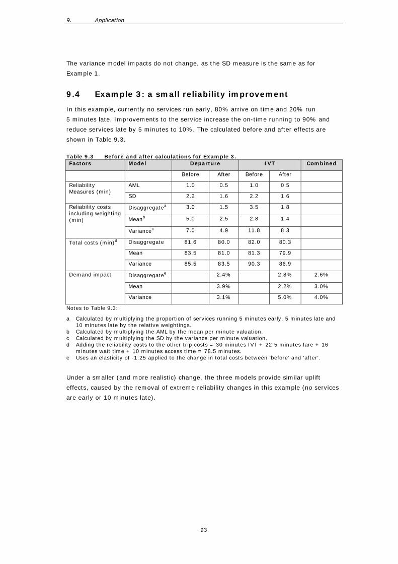
9. Application
93
The variance model impacts do not change, as the SD measure is the same as for
Example 1.
9.4 Example 3: a small reliability improvement
In this example, currently no services run early, 80% arrive on time and 20% run
5 minutes late. Improvements to the service increase the on-time running to 90% and
reduce services late by 5 minutes to 10%. The calculated before and after effects are
shown in Table 9.3.
Table 9.3 Before and after calculations for Example 3. Factors Model Departure IVT Combined
Before After Before After
AML 1.0 0.5 1.0 0.5 Reliability Measures (min)
SD 2.2 1.6 2.2 1.6
Disaggregatea 3.0 1.5 3.5 1.8
Meanb 5.0 2.5 2.8 1.4
Reliability costs including weighting (min)
Variancec 7.0 4.9 11.8 8.3
Disaggregate 81.6 80.0 82.0 80.3
Mean 83.5 81.0 81.3 79.9
Total costs (min)d
Variance 85.5 83.5 90.3 86.9
Disaggregatee 2.4% 2.8% 2.6%
Mean 3.9% 2.2% 3.0%
Demand impact
Variance 3.1% 5.0% 4.0%
Notes to Table 9.3:
a Calculated by multiplying the proportion of services running 5 minutes early, 5 minutes late and 10 minutes late by the relative weightings.
b Calculated by multiplying the AML by the mean per minute valuation. c Calculated by multiplying the SD by the variance per minute valuation. d Adding the reliability costs to the other trip costs = 30 minutes IVT + 22.5 minutes fare + 16
minutes wait time + 10 minutes access time = 78.5 minutes. e Uses an elasticity of -1.25 applied to the change in total costs between ‘before’ and ‘after’.
Under a smaller (and more realistic) change, the three models provide similar uplift
effects, caused by the removal of extreme reliability changes in this example (no services
are early or 10 minutes late).
MEASUREMENT VALUATION OF PUBLIC TRANSPORT RELIABILITY
94
9.5 Application within an Emme/2 modelling process
These three examples can be applied within an Emme/2 public transport model process
by using a combination of node and in-vehicle time adjustments. Any implemented
approach can be determined by the reliability information available. The recommended
approach is to use the mean model approach, where demand is based on average
reliability. An Emme/2 assignment process includes information on passengers waiting for
and travelling on services. As such, departure and in-vehicle variability could be
represented separately.
Assuming each service (or mode) has its own AML measure (from existing service
information) then reliability should be included in the transit assignment process. If the
AML is an average across the system (does not differ by mode), then reliability could be
included through a simple additional matrix calculation of the type shown in
Examples 1–3.
This could also be included in the assignment by taking an AML measure, and multiplying
it by the average of the departure and in-vehicle weights; subsequently, this could be
included as an additional boarding penalty in the assignment.
If, however, more detailed reliability information is available (such as the distribution of
reliability down a service, or differences by mode or service) then this measure can be
included in a transit line segment attribute. The segment would represent the change in
reliability between stations or stops on the network. Within the transit assignment, the
departure variability could be included by an additional boarding penalty based on the
sum of the segment values up to the point of boarding. This would then be multiplied by
the appropriate departure variability weighting to provide an additional penalty for
reliability. The in-vehicle reliability impact could be represented by including the AML
segment values in the transit time functions, again with the appropriate weights.
9. Application
95
10 Further work
We see the dataset that has been created as part of this study as a valuable resource for
further examination of reliability. In particular, the market could be segmented many
ways to provide further insight. Possible segmentations could be:
• by time of day,
• by service frequency,
• by trip length (IVT could be used as a proxy), or
• by inbound v. outbound valuations.
This study has also grouped shopping and social trips together in the ‘other’ group. We
have a sufficient amount of observations in these trip purposes to separate them in the
analysis if desired.
Collecting actual reliability service data and subsequently linking them with the valuations
would be a useful exercise to give a more accurate overall picture of the reliability
impacts.
Applying this methodology within specific transport models such as Wellington Transport
Strategy Model or the Auckland Public Transport model could be undertaken.
Finally, this study has not explored the impact of extreme levels of unreliability such as
delays greater than 10 minutes or service cancellations.
MEASUREMENT VALUATION OF PUBLIC TRANSPORT RELIABILITY
96
11 References
Algers, S., Dille, J. L., Widlert, S. 1995. The National Swedish Value of Time Study.
Swedish Institute for Transport and Communications Analysis (SIKA). 17 pp.
Auckland Regional Transport Authority. 2006. Auckland Passenger Transport Network
Plan. Auckland: Auckland Regional Transport Authority. 56 pp.
Australian Transport Council. 2006. National guidelines for transport system
management.
http://www.atcouncil.gov.au/documents/pubs/National_Guidelines_Volume_4.pdf.
Bates, J., Polak, J., Jones, P., Cook, A. 2001. The valuation of reliability for personal
travel. Transportation Research E 37(2-–): 191–229.
Bates, J., Jones, P., Polak, J., Han, X.-L. 1997. The Investigation of Punctuality and
Reliability: Re-analysis of Some Existing Datasets. Report submitted to Rail Operational
Research, University of Westminster, Transport Studies Group.
Beca Carter Hollings & Ferner Ltd. 2002. Review of Benefit Parameter Values for Economic
Evaluation. Wellington: Transfund New Zealand.
Bell, D. 2004. Dandenong Rail Corridor Market Assessment. Melbourne: Multi-modal
Transport Solutions.
Benwell, M., Black I. 1984. Train service reliability on BR InterCity services. Report 3:
Passenger Attitudes to Lateness. Cranfield University.
Benswell, M., Black, I. 1985. User Valuation of Reliability in Inter-urban Transport: Some
Problems of Measurement. Proceedings of Seminar L, PTRC Summer Annual Meeting,
Brighton, UK.
Black, I. G., Towriss, J. G. 1993. Demand Effects of Travel Time Reliability. Centre for
Logistics and Transportation: Cranfield Institute of Technology.
Booz Allen Hamilton. 2000. Valuation of public transport attributes. Transfund Research
Report 184. Wellington: Transfund New Zealand.
Booz Allen Hamilton. 2001. Sydney ferry business planning market research. Final report
prepared for State Transit, Australia. BAH Reference A2526.
11. References
97
Booz Allen Hamilton. 2002. PEM development project: impact of revised benefit
parameters on public transport evaluation. Final Report prepared for Transfund NZ. BAH
Reference Z1253.
Booz Allen Hamilton. 2006. Sunshine Corridor study market research. Final report
prepared for Department of Infrastructure, Victoria, Australia. BAH Reference A5133.
Client:
Blomquist, K., Jansson, K. 1995. Valuation of travel time and information – with and
without use of timetable (revised version). Paper presented at the 7th World Conference
on Transport Research, Sydney, July 1995.
Cook, A., Jones, P. M., Bates, J. J., Polak, J. W., Haigh, M. 1999. Improved methods of
representing travel time reliability in SP experiments. Proceedings of the 27th European
Transport Forum. London: PTRC.
De Jong, G. C., Daly, A. J., Pieters, M., Vellay, C., Bradley, M. A., Hofman, F. 2003. A
model for time of day and mode choice using error components logit. Transportation
Research E 39(3): 245–268.
De Jong, G., Kroes, E., Plasmeijer, R., Sanders, P., Warffemius, P. 2004. The Value of
Reliability. Paper presented at the Applied Methods stream, European Transport
Conference, Strasbourg, 4–6 October 2004.
Department for Transport (UK). 2006. Bus punctuality statistics GB: 2005.
http://www.dft.gov.uk/pgr/statistics/datatablespublications/public/buspunctuality/buspun
ctualitystatisticsgb2005a.
Department for Transport (UK). 2007a. Autumn performance report 2007.
http://www.dft.gov.uk/about/publications/apr/ap/autumnperformance07.pdf.
Department for Transport (UK). 2007b. Bus priority – the way ahead.
http://www.dft.gov.uk/pgr/regional/buses/bpf/busprioritythewayahead12/busprioritythew
ayaheadhtmlve1073
Department of Infrastructure (Victoria). 2007. Public transport – performance monitoring.
http://www.doi.vic.gov.au/doi/internet/transport.nsf/AllDocs/FE45C4AFFB575E49CA256E
7C00208161?OpenDocument#which.
Douglas, N. 1996. Sydney M2 Busway Patronage Forecasts. Report prepared for New
South Wales Department of Transport.
MEASUREMENT VALUATION OF PUBLIC TRANSPORT RELIABILITY
98
Douglas, N. 2005. Valuing Rail Service Quality – Sydney. Report prepared for RailCorp
NSW.
Geerts, J.-F., Haemers, V. 2004. Service Reliability and Transfer Convenience on the
Brussels Tramway Network. Paper presented at the European Transport Conference,
Strasbourg, October 2004.
Government of South Australia. 2005. Provision of bus services in the Outer North and/or
Outer North East and/or North South areas of Metropolitan Adelaide (DTUP010596).
http://www.tenders.sa.gov.au:80/tenders/contract/view.do?id=1304.
Hensher, D., Prioni, P. 2002. A service quality index for area-wide contract performance
assessment. Journal of Transport Economics and Policy 36: 93–113.
Hollander, Y. 2005a. Travellers’ Attitudes to Travel Time Variability: Intermodal and Intra-
modal Analysis. Paper presented at the 3rd International SIIV congress – People, Land,
Environment and Transport Infrastructure – Reliability and Development, September
2005, Bari, Italy.
Hollander, Y. 2005b. The Attitudes of Bus Users to Travel Time Variability. Paper
presented at the European Transport Conference, October 2005, Strasbourg, France.
Jackson, B. W., Jucker, J. V. 1982. An empirical study of travel time variability and travel
choice behavior. Transportation Science 16(4): 460–475.
Kouwenhoven, M., Caussade, S., Kroes, E. 2006. Value of reliability of travellers on the
Paris Suburban Railway Network.
http://www.rand.org/pubs/technical_reports/2006/RAND_TR223.pdf.
Land Transport New Zealand. 2005. Economic evaluation manual 2.
http://www.landtransport.govt.nz/funding/economic-evaluation-manual/eem2.pdf.
MVA Consultancy Ltd. 2000. Etude de l’Impact des Phénomènes d’Irregularité des
Autobus – Analyse des Resultants (Study of the Impact of the Phenomenon of Bus
Irregularity – Analysis of Results). Paris: MVA Consultancy Ltd.
Noland, R. B., Small, K. A., Koskenoja, P. M., Chu, X. 1998. Simulating travel reliability.
Regional Science and Urban Economics 28(5): 535–564.
Pells, S. 1987. The evaluation of reductions in the variability of travel times on the
journey to work. Pp 313–325 in Transportation Planning Methods, Proceedings of Seminar
C held at the PTRC Summer Annual Meeting, University of Bath, P290.
11. References
99
Polak, J., Hazelton, M. L. 1997 Bus Reliability Study – Stated Preference Research, Great
Britain. Draft final report to the Department of Transport, United Kingdom.
Rietveld, P., Bruinsma, F. R., van Vuuren, D. J. 2001. Coping with unreliability in public
transport chains: a case study for Netherlands. Transportation Research: Part A: Policy
and Practice 35(6): 539–559.
Rohr, P., Polak, J. W. 1998. The regularity and reliability impacts of bus priority
measures. Proceedings of the 26th European Transport Forum, PTRC, London.
Senna, L. A. D. S. 1994. The influence of travel time variability on the value of time.
Transportation 21: 203–228.
Small, K.A. 1982. The scheduling of consumer activities: work trips. American Economic
Review 72: 467–479.
Small, K., Noland, R., Koskenoja, P. 1995. Socio-economic Attributes and Impacts of
Travel Reliability: a Stated Preference Approach. California Partners for Advanced Transit
and Highways (PATH), Institute of Transportation Studies, University of California:
Berkeley, California.
Steer Davies & Gleave (NZ) Ltd. 1990. The Effects of Quality Improvements in Public
Transport. Report to Wellington Regional Council, November 1990.
Tilahun, N., Levinson, D. 2005. Travel Time Reliability in Route Choice using Adaptive
Stated Preference. Working Papers, Department of Civil Engineering, University of
Minnesota: Minnesota, USA.
Transport for London. 2007. Business Case Development Manual. London: Transport for
London Business Planning and Performance. 255 pp.
Wallis, I. 2005. Review of Bus Contracts – Performance Management Systems. Draft
report by Booz Allen Hamilton prepared for Transitlink, South Queensland.
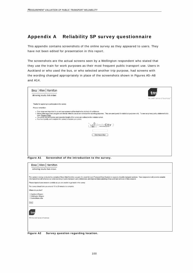
MEASUREMENT VALUATION OF PUBLIC TRANSPORT RELIABILITY
100
Appendix A Reliability SP survey questionnaire
This appendix contains screenshots of the online survey as they appeared to users. They
have not been edited for presentation in this report.
The screenshots are the actual screens seen by a Wellington respondent who stated that
they use the train for work purposes as their most frequent public transport use. Users in
Auckland or who used the bus, or who selected another trip purpose, had screens with
the wording changed appropriately in place of the screenshots shown in Figures A5–A8
and A14.
Figure A1 Screenshot of the introduction to the survey.
Figure A2 Survey question regarding location.
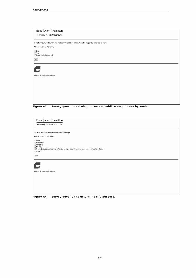
Appendices
101
Figure A3 Survey question relating to current public transport use by mode.
Figure A4 Survey question to determine trip purpose.
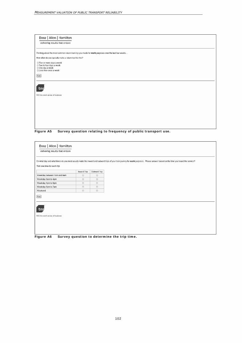
MEASUREMENT VALUATION OF PUBLIC TRANSPORT RELIABILITY
102
Figure A5 Survey question relating to frequency of public transport use.
Figure A6 Survey question to determine the trip time.
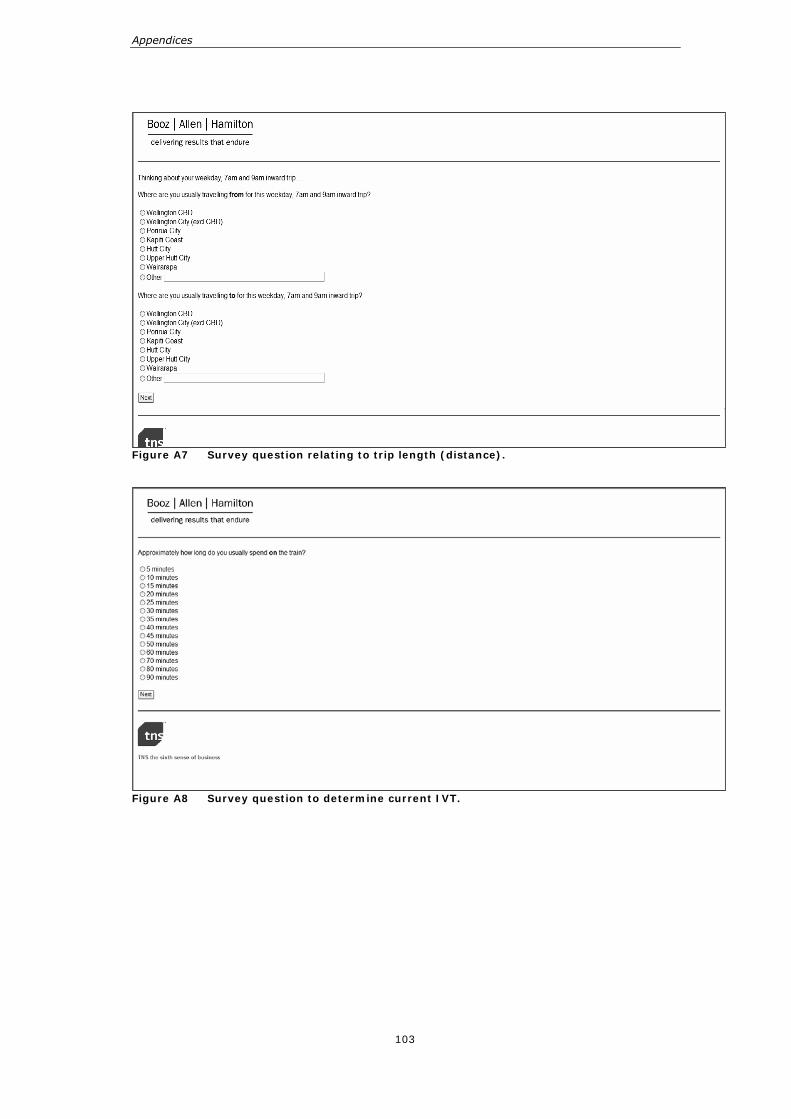
Appendices
103
Figure A7 Survey question relating to trip length (distance).
Figure A8 Survey question to determine current IVT.
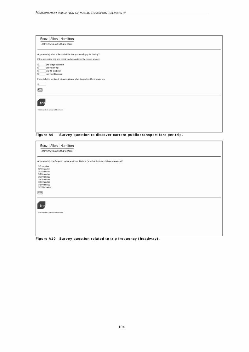
MEASUREMENT VALUATION OF PUBLIC TRANSPORT RELIABILITY
104
Figure A9 Survey question to discover current public transport fare per trip.
Figure A10 Survey question related to trip frequency (headway).
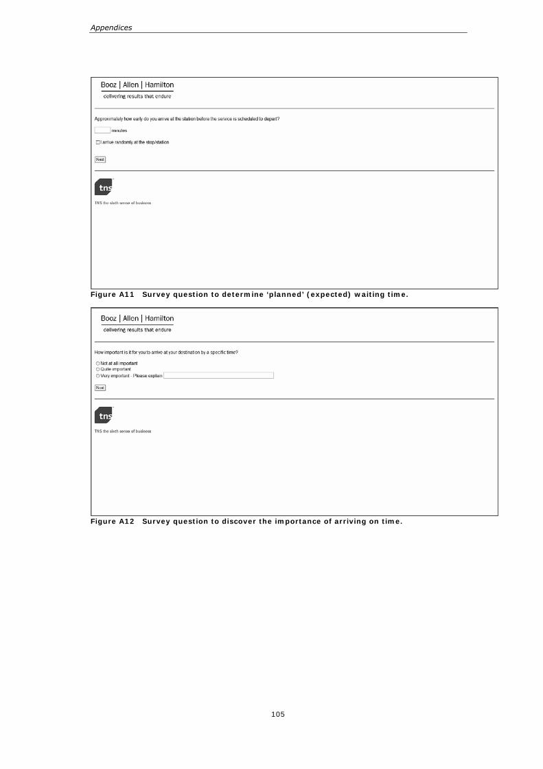
Appendices
105
Figure A11 Survey question to determine ‘planned’ (expected) waiting time.
Figure A12 Survey question to discover the importance of arriving on time.
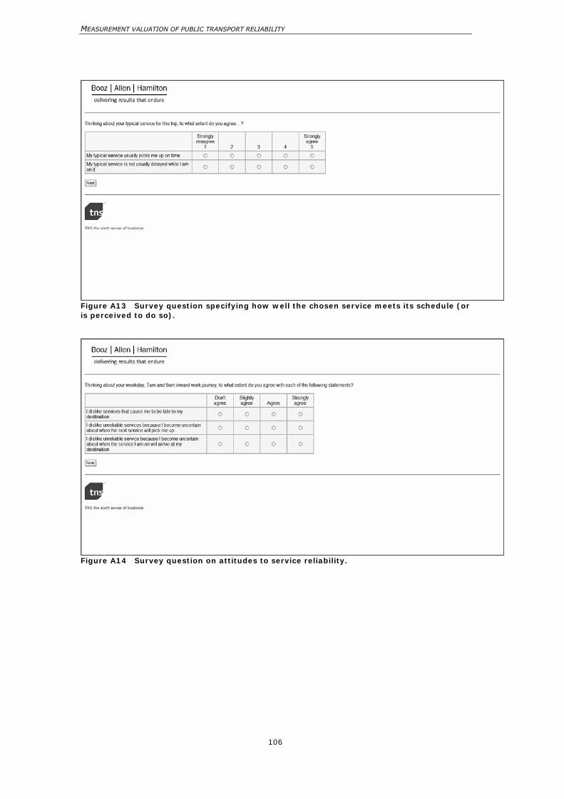
MEASUREMENT VALUATION OF PUBLIC TRANSPORT RELIABILITY
106
Figure A13 Survey question specifying how well the chosen service meets its schedule (or is perceived to do so).
Figure A14 Survey question on attitudes to service reliability.
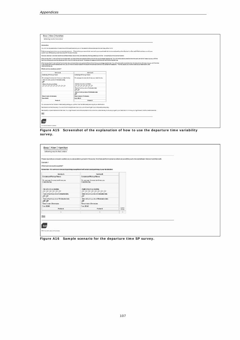
Appendices
107
Figure A15 Screenshot of the explanation of how to use the departure time variability survey.
Figure A16 Sample scenario for the departure time SP survey.
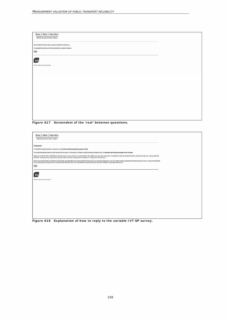
MEASUREMENT VALUATION OF PUBLIC TRANSPORT RELIABILITY
108
Figure A17 Screenshot of the ‘rest’ between questions.
Figure A18 Explanation of how to reply to the variable IVT SP survey.
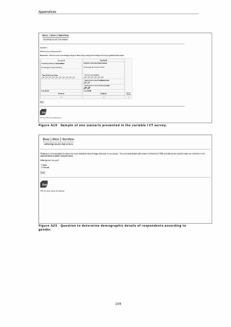
Appendices
109
Figure A19 Sample of one scenario presented in the variable IVT survey.
Figure A20 Question to determine demographic details of respondents according to gender.
MEASUREMENT VALUATION OF PUBLIC TRANSPORT RELIABILITY
110
Figure A21 Question to determine the age of respondents.
Figure A22 Question to determine the economic bracket of respondents.
Appendices
111
Figure A23 Screenshot of the form inviting further comments.
Figure A24 Screenshot of the complimentary closing to the survey.
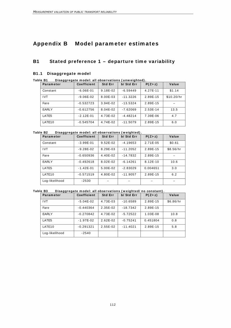
MEASUREMENT VALUATION OF PUBLIC TRANSPORT RELIABILITY
112
Appendix B Model parameter estimates
B1 Stated preference 1 – departure time variability
B1.1 Disaggregate model
Table B1 Disaggregate model: all observations (unweighted). Parameter Coefficient Std Err b/Std Err P(Z>z) Value
Constant -6.06E-01 9.18E-02 -6.59449 4.27E-11 $1.14
IVT -9.06E-02 8.00E-03 -11.3226 2.89E-15 $10.20/hr
Fare -0.532723 3.94E-02 -13.5324 2.89E-15 –
EARLY -0.612756 8.04E-02 -7.62069 2.53E-14 13.5
LATE5 -2.12E-01 4.73E-02 -4.48214 7.39E-06 4.7
LATE10 -0.545704 4.74E-02 -11.5079 2.89E-15 6.0
Table B2 Disaggregate model: all observations (weighted).
Parameter Coefficient Std Err b/Std Err P(Z>z) Value
Constant -3.99E-01 9.52E-02 -4.19653 2.71E-05 $0.61
IVT -9.28E-02 8.29E-03 -11.2052 2.89E-15 $8.56/hr
Fare -0.650936 4.40E-02 -14.7832 2.89E-15 –
EARLY -0.492618 8.02E-02 -6.14261 8.12E-10 10.6
LATE5 -1.42E-01 5.00E-02 -2.83029 0.004651 3.0
LATE10 -0.571519 4.80E-02 -11.9057 2.89E-15 6.2
Log-likelihood -2530 – – – –
Table B3 Disaggregate model: all observations (weighted/no constant).
Parameter Coefficient Std Err b/Std Err P(Z>z) Value
IVT -5.04E-02 4.73E-03 -10.6589 2.89E-15 $6.86/hr
Fare -0.440364 2.35E-02 -18.7342 2.89E-15
EARLY -0.270842 4.73E-02 -5.72522 1.03E-08 10.8
LATE5 -1.97E-02 2.62E-02 -0.75241 0.451804 0.8
LATE10 -0.291321 2.55E-02 -11.4021 2.89E-15 5.8
Log-likelihood -2540
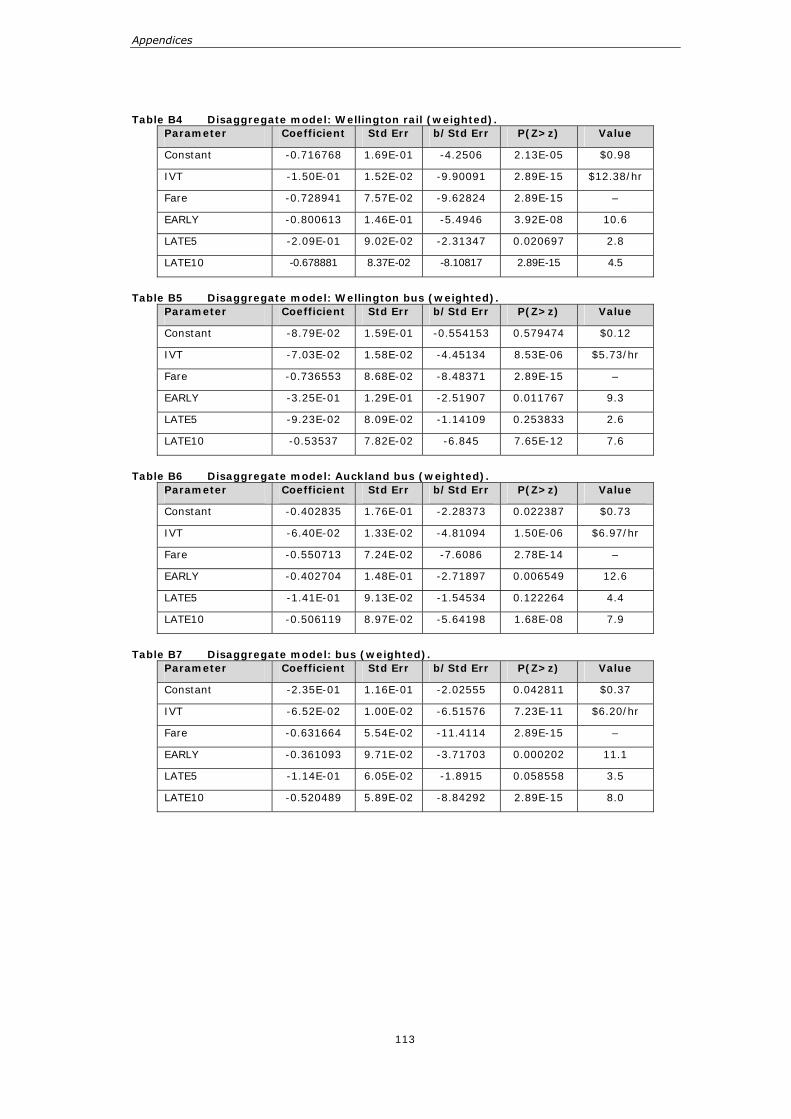
Appendices
113
Table B4 Disaggregate model: Wellington rail (weighted). Parameter Coefficient Std Err b/Std Err P(Z>z) Value
Constant -0.716768 1.69E-01 -4.2506 2.13E-05 $0.98
IVT -1.50E-01 1.52E-02 -9.90091 2.89E-15 $12.38/hr
Fare -0.728941 7.57E-02 -9.62824 2.89E-15 –
EARLY -0.800613 1.46E-01 -5.4946 3.92E-08 10.6
LATE5 -2.09E-01 9.02E-02 -2.31347 0.020697 2.8
LATE10 -0.678881 8.37E-02 -8.10817 2.89E-15 4.5
Table B5 Disaggregate model: Wellington bus (weighted).
Parameter Coefficient Std Err b/Std Err P(Z>z) Value
Constant -8.79E-02 1.59E-01 -0.554153 0.579474 $0.12
IVT -7.03E-02 1.58E-02 -4.45134 8.53E-06 $5.73/hr
Fare -0.736553 8.68E-02 -8.48371 2.89E-15 –
EARLY -3.25E-01 1.29E-01 -2.51907 0.011767 9.3
LATE5 -9.23E-02 8.09E-02 -1.14109 0.253833 2.6
LATE10 -0.53537 7.82E-02 -6.845 7.65E-12 7.6
Table B6 Disaggregate model: Auckland bus (weighted).
Parameter Coefficient Std Err b/Std Err P(Z>z) Value
Constant -0.402835 1.76E-01 -2.28373 0.022387 $0.73
IVT -6.40E-02 1.33E-02 -4.81094 1.50E-06 $6.97/hr
Fare -0.550713 7.24E-02 -7.6086 2.78E-14 –
EARLY -0.402704 1.48E-01 -2.71897 0.006549 12.6
LATE5 -1.41E-01 9.13E-02 -1.54534 0.122264 4.4
LATE10 -0.506119 8.97E-02 -5.64198 1.68E-08 7.9
Table B7 Disaggregate model: bus (weighted).
Parameter Coefficient Std Err b/Std Err P(Z>z) Value
Constant -2.35E-01 1.16E-01 -2.02555 0.042811 $0.37
IVT -6.52E-02 1.00E-02 -6.51576 7.23E-11 $6.20/hr
Fare -0.631664 5.54E-02 -11.4114 2.89E-15 –
EARLY -0.361093 9.71E-02 -3.71703 0.000202 11.1
LATE5 -1.14E-01 6.05E-02 -1.8915 0.058558 3.5
LATE10 -0.520489 5.89E-02 -8.84292 2.89E-15 8.0
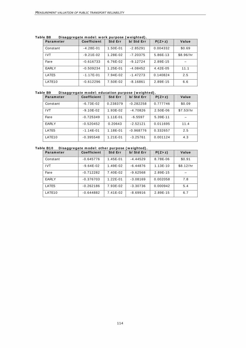
MEASUREMENT VALUATION OF PUBLIC TRANSPORT RELIABILITY
114
Table B8 Disaggregate model: work purpose (weighted). Parameter Coefficient Std Err b/Std Err P(Z>z) Value
Constant -4.28E-01 1.50E-01 -2.85291 0.004332 $0.69
IVT -9.21E-02 1.28E-02 -7.20375 5.86E-13 $8.96/hr
Fare -0.616733 6.76E-02 -9.12724 2.89E-15 –
EARLY -0.509234 1.25E-01 -4.08452 4.42E-05 11.1
LATE5 -1.17E-01 7.94E-02 -1.47273 0.140824 2.5
LATE10 -0.612296 7.50E-02 -8.16861 2.89E-15 6.6
Table B9 Disaggregate model: education purpose (weighted).
Parameter Coefficient Std Err b/Std Err P(Z>z) Value
Constant -6.73E-02 0.238379 -0.282258 0.777746 $0.09
IVT -9.10E-02 1.93E-02 -4.70826 2.50E-06 $7.53/hr
Fare -0.725349 1.11E-01 -6.5597 5.39E-11 –
EARLY -0.520452 0.20643 -2.52121 0.011695 11.4
LATE5 -1.14E-01 1.18E-01 -0.968776 0.332657 2.5
LATE10 -0.395548 1.21E-01 -3.25761 0.001124 4.3
Table B10 Disaggregate model: other purpose (weighted).
Parameter Coefficient Std Err b/Std Err P(Z>z) Value
Constant -0.645776 1.45E-01 -4.44529 8.78E-06 $0.91
IVT -9.64E-02 1.49E-02 -6.44876 1.13E-10 $8.12/hr
Fare -0.712282 7.40E-02 -9.62568 2.89E-15 –
EARLY -0.376703 1.22E-01 -3.08169 0.002058 7.8
LATE5 -0.262186 7.93E-02 -3.30736 0.000942 5.4
LATE10 -0.644882 7.41E-02 -8.69916 2.89E-15 6.7
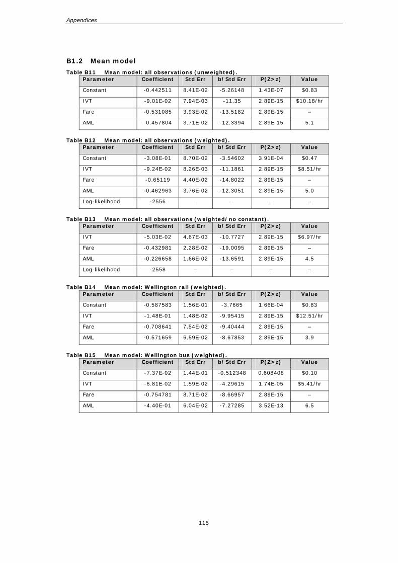
Appendices
115
B1.2 Mean model
Table B11 Mean model: all observations (unweighted). Parameter Coefficient Std Err b/Std Err P(Z>z) Value
Constant -0.442511 8.41E-02 -5.26148 1.43E-07 $0.83
IVT -9.01E-02 7.94E-03 -11.35 2.89E-15 $10.18/hr
Fare -0.531085 3.93E-02 -13.5182 2.89E-15 –
AML -0.457804 3.71E-02 -12.3394 2.89E-15 5.1
Table B12 Mean model: all observations (weighted).
Parameter Coefficient Std Err b/Std Err P(Z>z) Value
Constant -3.08E-01 8.70E-02 -3.54602 3.91E-04 $0.47
IVT -9.24E-02 8.26E-03 -11.1861 2.89E-15 $8.51/hr
Fare -0.65119 4.40E-02 -14.8022 2.89E-15 –
AML -0.462963 3.76E-02 -12.3051 2.89E-15 5.0
Log-likelihood -2556 – – – –
Table B13 Mean model: all observations (weighted/no constant).
Parameter Coefficient Std Err b/Std Err P(Z>z) Value
IVT -5.03E-02 4.67E-03 -10.7727 2.89E-15 $6.97/hr
Fare -0.432981 2.28E-02 -19.0095 2.89E-15 –
AML -0.226658 1.66E-02 -13.6591 2.89E-15 4.5
Log-likelihood -2558 – – – –
Table B14 Mean model: Wellington rail (weighted).
Parameter Coefficient Std Err b/Std Err P(Z>z) Value
Constant -0.587583 1.56E-01 -3.7665 1.66E-04 $0.83
IVT -1.48E-01 1.48E-02 -9.95415 2.89E-15 $12.51/hr
Fare -0.708641 7.54E-02 -9.40444 2.89E-15 –
AML -0.571659 6.59E-02 -8.67853 2.89E-15 3.9
Table B15 Mean model: Wellington bus (weighted).
Parameter Coefficient Std Err b/Std Err P(Z>z) Value
Constant -7.37E-02 1.44E-01 -0.512348 0.608408 $0.10
IVT -6.81E-02 1.59E-02 -4.29615 1.74E-05 $5.41/hr
Fare -0.754781 8.71E-02 -8.66957 2.89E-15 –
AML -4.40E-01 6.04E-02 -7.27285 3.52E-13 6.5
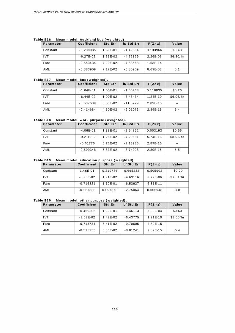
MEASUREMENT VALUATION OF PUBLIC TRANSPORT RELIABILITY
116
Table B16 Mean model: Auckland bus (weighted).
Parameter Coefficient Std Err b/Std Err P(Z>z) Value
Constant -0.238985 1.59E-01 -1.49864 0.133966 $0.43
IVT -6.27E-02 1.33E-02 -4.72829 2.26E-06 $6.80/hr
Fare -0.553434 7.20E-02 -7.68568 1.53E-14 –
AML -0.383909 7.17E-02 -5.35209 8.69E-08 6.1
Table B17 Mean model: bus (weighted).
Parameter Coefficient Std Err b/Std Err P(Z>z) Value
Constant -1.64E-01 1.05E-01 -1.55968 0.118835 $0.26
IVT -6.44E-02 1.00E-02 -6.43434 1.24E-10 $6.06/hr
Fare -0.637639 5.53E-02 -11.5229 2.89E-15 –
AML -0.414684 4.60E-02 -9.01073 2.89E-15 6.4
Table B18 Mean model: work purpose (weighted).
Parameter Coefficient Std Err b/Std Err P(Z>z) Value
Constant -4.06E-01 1.38E-01 -2.94852 0.003193 $0.66
IVT -9.21E-02 1.28E-02 -7.20651 5.74E-13 $8.95/hr
Fare -0.61775 6.76E-02 -9.13285 2.89E-15 –
AML -0.509348 5.83E-02 -8.74028 2.89E-15 5.5
Table B19 Mean model: education purpose (weighted).
Parameter Coefficient Std Err b/Std Err P(Z>z) Value
Constant 1.46E-01 0.219786 0.665232 0.505902 -$0.20
IVT -8.98E-02 1.91E-02 -4.69116 2.72E-06 $7.51/hr
Fare -0.716821 1.10E-01 -6.53627 6.31E-11 –
AML -0.267838 0.097373 -2.75064 0.005948 3.0
Table B20 Mean model: other purpose (weighted).
Parameter Coefficient Std Err b/Std Err P(Z>z) Value
Constant -0.450305 1.30E-01 -3.46113 5.38E-04 $0.63
IVT -9.58E-02 1.49E-02 -6.43775 1.21E-10 $8.00/hr
Fare -0.718734 7.41E-02 -9.70605 2.89E-15 –
AML -0.515233 5.85E-02 -8.81241 2.89E-15 5.4
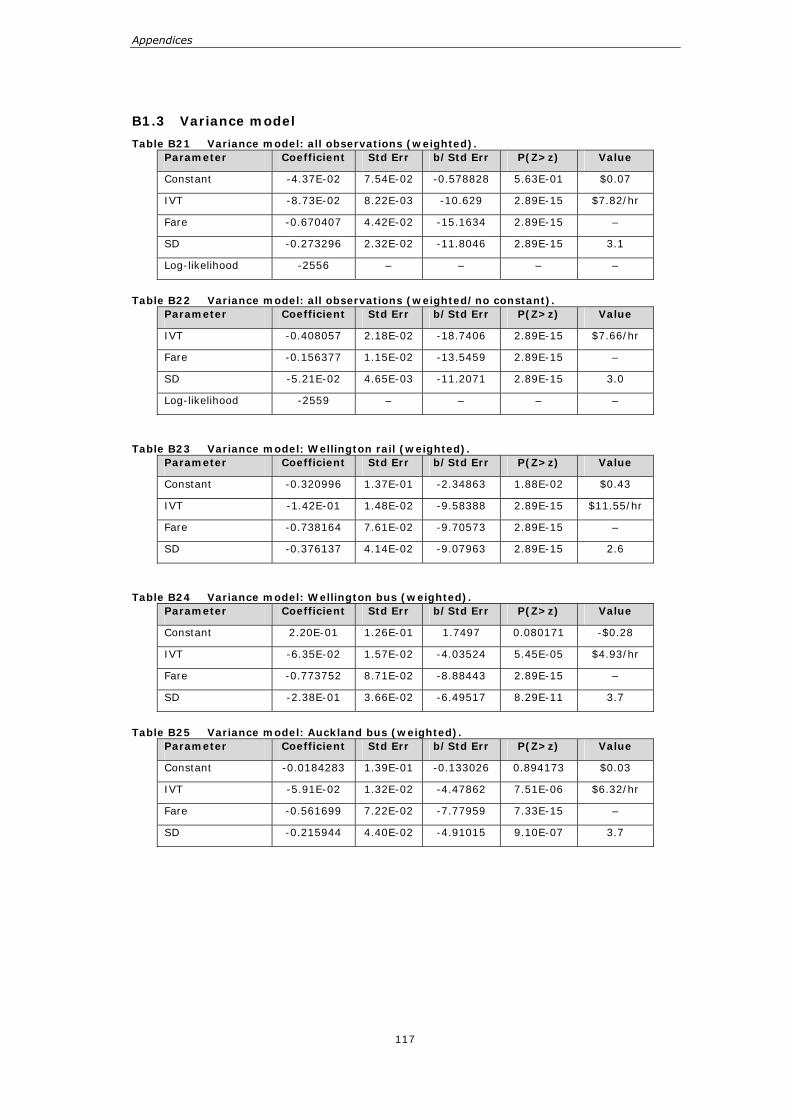
Appendices
117
B1.3 Variance model
Table B21 Variance model: all observations (weighted). Parameter Coefficient Std Err b/Std Err P(Z>z) Value
Constant -4.37E-02 7.54E-02 -0.578828 5.63E-01 $0.07
IVT -8.73E-02 8.22E-03 -10.629 2.89E-15 $7.82/hr
Fare -0.670407 4.42E-02 -15.1634 2.89E-15 –
SD -0.273296 2.32E-02 -11.8046 2.89E-15 3.1
Log-likelihood -2556 – – – –
Table B22 Variance model: all observations (weighted/no constant).
Parameter Coefficient Std Err b/Std Err P(Z>z) Value
IVT -0.408057 2.18E-02 -18.7406 2.89E-15 $7.66/hr
Fare -0.156377 1.15E-02 -13.5459 2.89E-15 –
SD -5.21E-02 4.65E-03 -11.2071 2.89E-15 3.0
Log-likelihood -2559 – – – –
Table B23 Variance model: Wellington rail (weighted).
Parameter Coefficient Std Err b/Std Err P(Z>z) Value
Constant -0.320996 1.37E-01 -2.34863 1.88E-02 $0.43
IVT -1.42E-01 1.48E-02 -9.58388 2.89E-15 $11.55/hr
Fare -0.738164 7.61E-02 -9.70573 2.89E-15 –
SD -0.376137 4.14E-02 -9.07963 2.89E-15 2.6
Table B24 Variance model: Wellington bus (weighted).
Parameter Coefficient Std Err b/Std Err P(Z>z) Value
Constant 2.20E-01 1.26E-01 1.7497 0.080171 -$0.28
IVT -6.35E-02 1.57E-02 -4.03524 5.45E-05 $4.93/hr
Fare -0.773752 8.71E-02 -8.88443 2.89E-15 –
SD -2.38E-01 3.66E-02 -6.49517 8.29E-11 3.7
Table B25 Variance model: Auckland bus (weighted).
Parameter Coefficient Std Err b/Std Err P(Z>z) Value
Constant -0.0184283 1.39E-01 -0.133026 0.894173 $0.03
IVT -5.91E-02 1.32E-02 -4.47862 7.51E-06 $6.32/hr
Fare -0.561699 7.22E-02 -7.77959 7.33E-15 –
SD -0.215944 4.40E-02 -4.91015 9.10E-07 3.7
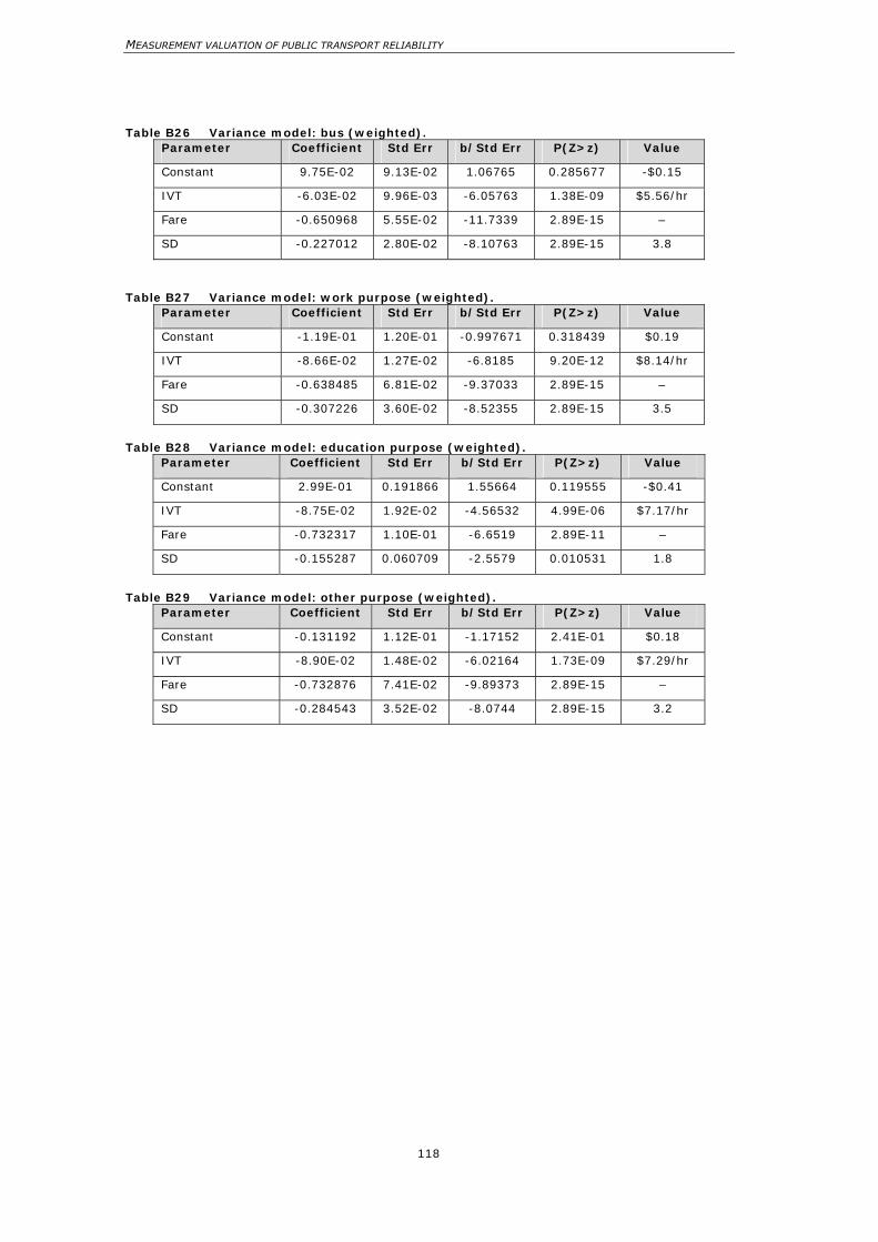
MEASUREMENT VALUATION OF PUBLIC TRANSPORT RELIABILITY
118
Table B26 Variance model: bus (weighted). Parameter Coefficient Std Err b/Std Err P(Z>z) Value
Constant 9.75E-02 9.13E-02 1.06765 0.285677 -$0.15
IVT -6.03E-02 9.96E-03 -6.05763 1.38E-09 $5.56/hr
Fare -0.650968 5.55E-02 -11.7339 2.89E-15 –
SD -0.227012 2.80E-02 -8.10763 2.89E-15 3.8
Table B27 Variance model: work purpose (weighted).
Parameter Coefficient Std Err b/Std Err P(Z>z) Value
Constant -1.19E-01 1.20E-01 -0.997671 0.318439 $0.19
IVT -8.66E-02 1.27E-02 -6.8185 9.20E-12 $8.14/hr
Fare -0.638485 6.81E-02 -9.37033 2.89E-15 –
SD -0.307226 3.60E-02 -8.52355 2.89E-15 3.5
Table B28 Variance model: education purpose (weighted).
Parameter Coefficient Std Err b/Std Err P(Z>z) Value
Constant 2.99E-01 0.191866 1.55664 0.119555 -$0.41
IVT -8.75E-02 1.92E-02 -4.56532 4.99E-06 $7.17/hr
Fare -0.732317 1.10E-01 -6.6519 2.89E-11 –
SD -0.155287 0.060709 -2.5579 0.010531 1.8
Table B29 Variance model: other purpose (weighted).
Parameter Coefficient Std Err b/Std Err P(Z>z) Value
Constant -0.131192 1.12E-01 -1.17152 2.41E-01 $0.18
IVT -8.90E-02 1.48E-02 -6.02164 1.73E-09 $7.29/hr
Fare -0.732876 7.41E-02 -9.89373 2.89E-15 –
SD -0.284543 3.52E-02 -8.0744 2.89E-15 3.2
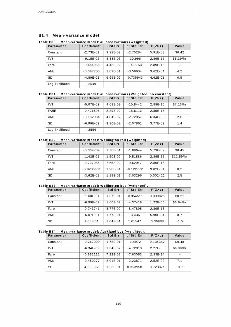
Appendices
119
B1.4 Mean-variance model
Table B30 Mean-variance model: all observations (weighted). Parameter Coefficient Std Err b/Std Err P(Z>z) Value
Constant -2.73E-01 9.92E-02 -2.75284 5.91E-03 $0.42
IVT -9.15E-02 8.33E-03 -10.996 2.89E-15 $8.39/hr
Fare -0.654956 4.43E-02 -14.7753 2.89E-15 –
AML -0.387705 1.09E-01 -3.56634 3.62E-04 4.2
SD -4.89E-02 6.65E-02 -0.735943 4.62E-01 0.5
Log-likelihood -2549 – – – –
Table B31 Mean-variance model: all observations (Weighted/no constant).
Parameter Coefficient Std Err b/Std Err P(Z>z) Value
IVT -5.07E-02 4.68E-03 -10.8442 2.89E-15 $7.13/hr
FARE -0.426898 2.29E-02 -18.6113 2.89E-15 –
AML -0.132034 4.84E-02 -2.72957 6.34E-03 2.6
SD -6.99E-02 3.36E-02 -2.07861 3.77E-02 1.4
Log-likelihood -2556 – – – –
Table B32 Mean-variance model: Wellington rail (weighted).
Parameter Coefficient Std Err b/Std Err P(Z>z) Value
Constant -0.334709 1.76E-01 -1.89644 5.79E-02 $0.45
IVT -1.42E-01 1.50E-02 -9.51886 2.89E-15 $11.59/hr
Fare -0.737086 7.65E-02 -9.62947 2.89E-15 –
AML -0.0233001 1.90E-01 -0.122772 9.02E-01 0.2
SD -3.62E-01 1.19E-01 -3.03296 0.002422 2.5
Table B33 Mean-variance model: Wellington bus (weighted).
Parameter Coefficient Std Err b/Std Err P(Z>z) Value
Constant -1.60E-01 1.67E-01 -0.954511 0.339825 $0.21
IVT -6.99E-02 1.60E-02 -4.37418 1.22E-05 $5.64/hr
Fare -0.743741 8.77E-02 -8.47895 2.89E-15 –
AML -6.07E-01 1.77E-01 -3.436 5.90E-04 8.7
SD 1.06E-01 1.04E-01 1.01547 0.30988 -1.5
Table B34 Mean-variance model: Auckland bus (weighted).
Parameter Coefficient Std Err b/Std Err P(Z>z) Value
Constant -0.267009 1.78E-01 -1.4972 0.134342 $0.48
IVT -6.34E-02 1.34E-02 -4.72813 2.27E-06 $6.90/hr
Fare -0.551212 7.22E-02 -7.63053 2.33E-14 –
AML -0.450277 2.01E-01 -2.23871 2.52E-02 7.1
SD 4.35E-02 1.23E-01 0.353958 0.723371 -0.7
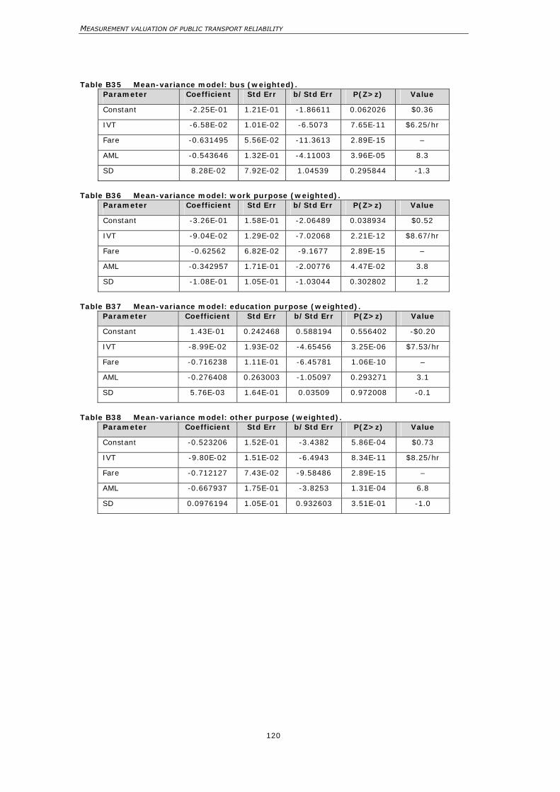
MEASUREMENT VALUATION OF PUBLIC TRANSPORT RELIABILITY
120
Table B35 Mean-variance model: bus (weighted). Parameter Coefficient Std Err b/Std Err P(Z>z) Value
Constant -2.25E-01 1.21E-01 -1.86611 0.062026 $0.36
IVT -6.58E-02 1.01E-02 -6.5073 7.65E-11 $6.25/hr
Fare -0.631495 5.56E-02 -11.3613 2.89E-15 –
AML -0.543646 1.32E-01 -4.11003 3.96E-05 8.3
SD 8.28E-02 7.92E-02 1.04539 0.295844 -1.3
Table B36 Mean-variance model: work purpose (weighted).
Parameter Coefficient Std Err b/Std Err P(Z>z) Value
Constant -3.26E-01 1.58E-01 -2.06489 0.038934 $0.52
IVT -9.04E-02 1.29E-02 -7.02068 2.21E-12 $8.67/hr
Fare -0.62562 6.82E-02 -9.1677 2.89E-15 –
AML -0.342957 1.71E-01 -2.00776 4.47E-02 3.8
SD -1.08E-01 1.05E-01 -1.03044 0.302802 1.2
Table B37 Mean-variance model: education purpose (weighted).
Parameter Coefficient Std Err b/Std Err P(Z>z) Value
Constant 1.43E-01 0.242468 0.588194 0.556402 -$0.20
IVT -8.99E-02 1.93E-02 -4.65456 3.25E-06 $7.53/hr
Fare -0.716238 1.11E-01 -6.45781 1.06E-10 –
AML -0.276408 0.263003 -1.05097 0.293271 3.1
SD 5.76E-03 1.64E-01 0.03509 0.972008 -0.1
Table B38 Mean-variance model: other purpose (weighted).
Parameter Coefficient Std Err b/Std Err P(Z>z) Value
Constant -0.523206 1.52E-01 -3.4382 5.86E-04 $0.73
IVT -9.80E-02 1.51E-02 -6.4943 8.34E-11 $8.25/hr
Fare -0.712127 7.43E-02 -9.58486 2.89E-15 –
AML -0.667937 1.75E-01 -3.8253 1.31E-04 6.8
SD 0.0976194 1.05E-01 0.932603 3.51E-01 -1.0
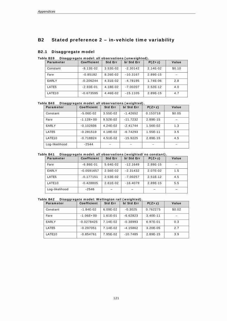
Appendices
121
B2 Stated preference 2 – in-vehicle time variability
B2.1 Disaggregate model
Table B39 Disaggregate model: all observations (unweighted). Parameter Coefficient Std Err b/Std Err P(Z>z) Value
Constant -8.13E-02 3.53E-02 -2.30142 2.14E-02 $0.10
Fare -0.85182 8.26E-02 -10.3167 2.89E-15 –
EARLY -0.206244 4.31E-02 -4.78195 1.74E-06 2.8
LATE5 -2.93E-01 4.18E-02 -7.00207 2.52E-12 4.0
LATE10 -0.673595 4.46E-02 -15.1105 2.89E-15 4.7
Table B40 Disaggregate model: all observations (weighted).
Parameter Coefficient Std Err b/Std Err P(Z>z) Value
Constant -5.06E-02 3.55E-02 -1.42652 0.153718 $0.05
Fare -1.12E+00 9.52E-02 -11.7232 2.89E-15 –
EARLY -0.102606 4.24E-02 -2.41744 1.56E-02 1.3
LATE5 -0.281519 4.18E-02 -6.74293 1.55E-11 3.5
LATE10 -0.718824 4.51E-02 -15.9225 2.89E-15 4.5
Log-likelihood -2544 – – – –
Table B41 Disaggregate model: all observations (weighted/no constant).
Parameter Coefficient Std Err b/Std Err P(Z>z) Value
Fare -6.86E-01 5.64E-02 -12.1649 2.89E-15 –
EARLY -0.0591657 2.56E-02 -2.31432 2.07E-02 1.5
LATE5 -0.177151 2.53E-02 -7.00257 2.51E-12 4.5
LATE10 -0.428805 2.61E-02 -16.4079 2.89E-15 5.5
Log-likelihood -2546 – – – –
Table B42 Disaggregate model: Wellington rail (weighted).
Parameter Coefficient Std Err b/Std Err P(Z>z) Value
Constant -1.84E-02 6.09E-02 -0.3025 0.762275 $0.02
Fare -1.06E+00 1.61E-01 -6.62823 3.40E-11 –
EARLY -0.0278425 7.14E-02 -0.38993 6.97E-01 0.3
LATE5 -0.297051 7.14E-02 -4.15862 3.20E-05 2.7
LATE10 -0.854761 7.95E-02 -10.7485 2.89E-15 3.9
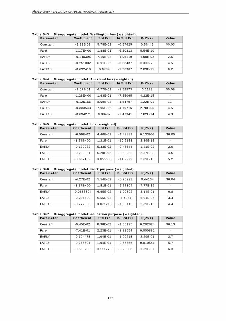
MEASUREMENT VALUATION OF PUBLIC TRANSPORT RELIABILITY
122
Table B43 Disaggregate model: Wellington bus (weighted). Parameter Coefficient Std Err b/Std Err P(Z>z) Value
Constant -3.33E-02 5.78E-02 -0.57625 0.56445 $0.03
Fare -1.17E+00 1.88E-01 -6.20313 5.54E-10 –
EARLY -0.140395 7.16E-02 -1.96119 4.99E-02 2.5
LATE5 -0.251002 6.91E-02 -3.63437 0.000279 4.5
LATE10 -0.692419 0.0739 -9.36967 2.89E-15 6.2
Table B44 Disaggregate model: Auckland bus (weighted).
Parameter Coefficient Std Err b/Std Err P(Z>z) Value
Constant -1.07E-01 6.77E-02 -1.58573 0.1128 $0.08
Fare -1.28E+00 1.63E-01 -7.85065 4.22E-15 –
EARLY -0.125166 8.09E-02 -1.54797 1.22E-01 1.7
LATE5 -0.333543 7.95E-02 -4.19716 2.70E-05 4.5
LATE10 -0.634271 0.08487 -7.47341 7.82E-14 4.3
Table B45 Disaggregate model: bus (weighted).
Parameter Coefficient Std Err b/Std Err P(Z>z) Value
Constant -6.59E-02 4.40E-02 -1.49889 0.133903 $0.05
Fare -1.24E+00 1.21E-01 -10.2153 2.89E-15 –
EARLY -0.130982 5.33E-02 -2.45544 1.41E-02 2.0
LATE5 -0.290061 5.20E-02 -5.58262 2.37E-08 4.5
LATE10 -0.667152 0.055606 -11.9979 2.89E-15 5.2
Table B46 Disaggregate model: work purpose (weighted).
Parameter Coefficient Std Err b/Std Err P(Z>z) Value
Constant -4.27E-02 5.54E-02 -0.76993 0.44134 $0.04
Fare -1.17E+00 1.51E-01 -7.77304 7.77E-15 –
EARLY -0.0668604 6.65E-02 -1.00592 3.14E-01 0.8
LATE5 -0.294689 6.55E-02 -4.4964 6.91E-06 3.4
LATE10 -0.772058 0.071213 -10.8415 2.89E-15 4.4
Table B47 Disaggregate model: education purpose (weighted).
Parameter Coefficient Std Err b/Std Err P(Z>z) Value
Constant -9.45E-02 8.98E-02 -1.05195 0.292824 $0.13
Fare -7.41E-01 2.23E-01 -3.32554 0.000882 –
EARLY -0.124475 1.04E-01 -1.20215 2.29E-01 2.7
LATE5 -0.265604 1.04E-01 -2.55756 0.010541 5.7
LATE10 -0.588706 0.111775 -5.26688 1.39E-07 6.3
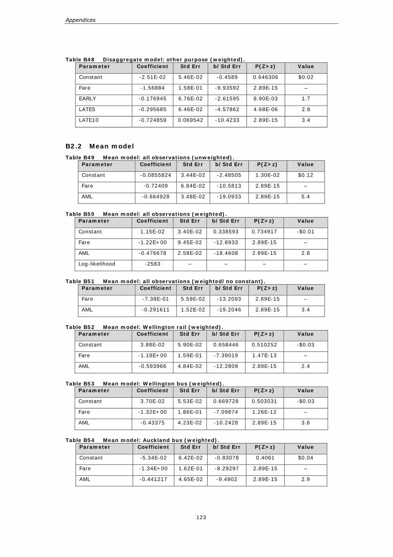
Appendices
123
Table B48 Disaggregate model: other purpose (weighted). Parameter Coefficient Std Err b/Std Err P(Z>z) Value
Constant -2.51E-02 5.46E-02 -0.4589 0.646306 $0.02
Fare -1.56884 1.58E-01 -9.93592 2.89E-15 –
EARLY -0.176945 6.76E-02 -2.61595 8.90E-03 1.7
LATE5 -0.295685 6.46E-02 -4.57862 4.68E-06 2.8
LATE10 -0.724859 0.069542 -10.4233 2.89E-15 3.4
B2.2 Mean model
Table B49 Mean model: all observations (unweighted). Parameter Coefficient Std Err b/Std Err P(Z>z) Value
Constant -0.0855824 3.44E-02 -2.48505 1.30E-02 $0.12
Fare -0.72409 6.84E-02 -10.5813 2.89E-15 –
AML -0.664928 3.48E-02 -19.0933 2.89E-15 5.4
Table B50 Mean model: all observations (weighted).
Parameter Coefficient Std Err b/Std Err P(Z>z) Value
Constant 1.15E-02 3.40E-02 0.338593 0.734917 -$0.01
Fare -1.22E+00 9.45E-02 -12.8933 2.89E-15 –
AML -0.476678 2.58E-02 -18.4608 2.89E-15 2.8
Log-likelihood -2583 – – – –
Table B51 Mean model: all observations (weighted/no constant).
Parameter Coefficient Std Err b/Std Err P(Z>z) Value
Fare -7.38E-01 5.59E-02 -13.2093 2.89E-15 –
AML -0.291611 1.52E-02 -19.2046 2.89E-15 3.4
Table B52 Mean model: Wellington rail (weighted).
Parameter Coefficient Std Err b/Std Err P(Z>z) Value
Constant 3.88E-02 5.90E-02 0.658446 0.510252 -$0.03
Fare -1.18E+00 1.59E-01 -7.39019 1.47E-13 –
AML -0.593966 4.84E-02 -12.2809 2.89E-15 2.4
Table B53 Mean model: Wellington bus (weighted).
Parameter Coefficient Std Err b/Std Err P(Z>z) Value
Constant 3.70E-02 5.53E-02 0.669728 0.503031 -$0.03
Fare -1.32E+00 1.86E-01 -7.09874 1.26E-12 –
AML -0.43375 4.23E-02 -10.2428 2.89E-15 3.6
Table B54 Mean model: Auckland bus (weighted).
Parameter Coefficient Std Err b/Std Err P(Z>z) Value
Constant -5.34E-02 6.42E-02 -0.83078 0.4061 $0.04
Fare -1.34E+00 1.62E-01 -8.29297 2.89E-15 –
AML -0.441217 4.65E-02 -9.4902 2.89E-15 2.9
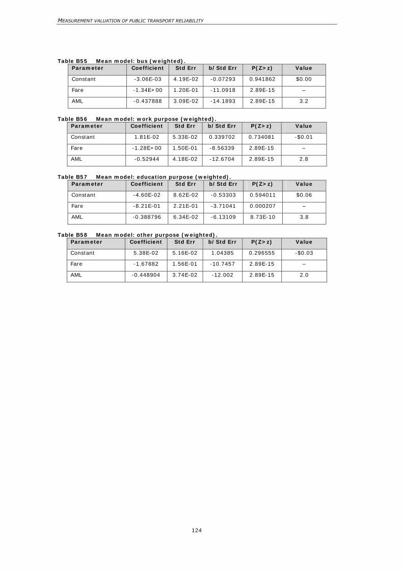
MEASUREMENT VALUATION OF PUBLIC TRANSPORT RELIABILITY
124
Table B55 Mean model: bus (weighted). Parameter Coefficient Std Err b/Std Err P(Z>z) Value
Constant -3.06E-03 4.19E-02 -0.07293 0.941862 $0.00
Fare -1.34E+00 1.20E-01 -11.0918 2.89E-15 –
AML -0.437888 3.09E-02 -14.1893 2.89E-15 3.2
Table B56 Mean model: work purpose (weighted).
Parameter Coefficient Std Err b/Std Err P(Z>z) Value
Constant 1.81E-02 5.33E-02 0.339702 0.734081 -$0.01
Fare -1.28E+00 1.50E-01 -8.56339 2.89E-15 –
AML -0.52944 4.18E-02 -12.6704 2.89E-15 2.8
Table B57 Mean model: education purpose (weighted).
Parameter Coefficient Std Err b/Std Err P(Z>z) Value
Constant -4.60E-02 8.62E-02 -0.53303 0.594011 $0.06
Fare -8.21E-01 2.21E-01 -3.71041 0.000207 –
AML -0.388796 6.34E-02 -6.13109 8.73E-10 3.8
Table B58 Mean model: other purpose (weighted).
Parameter Coefficient Std Err b/Std Err P(Z>z) Value
Constant 5.38E-02 5.16E-02 1.04385 0.296555 -$0.03
Fare -1.67882 1.56E-01 -10.7457 2.89E-15 –
AML -0.448904 3.74E-02 -12.002 2.89E-15 2.0
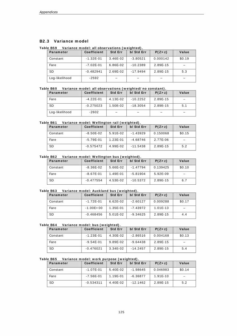
Appendices
125
B2.3 Variance model
Table B59 Variance model: all observations (weighted). Parameter Coefficient Std Err b/Std Err P(Z>z) Value
Constant -1.32E-01 3.46E-02 -3.80521 0.000142 $0.19
Fare -7.02E-01 6.86E-02 -10.2389 2.89E-15 –
SD -0.482941 2.69E-02 -17.9494 2.89E-15 5.3
Log-likelihood -2592 – – – –
Table B60 Variance model: all observations (weighted/no constant).
Parameter Coefficient Std Err b/Std Err P(Z>z) Value
Fare -4.22E-01 4.13E-02 -10.2252 2.89E-15 –
SD -0.275023 1.50E-02 -18.3054 2.89E-15 5.1
Log-likelihood -2602 – – – –
Table B61 Variance model: Wellington rail (weighted).
Parameter Coefficient Std Err b/Std Err P(Z>z) Value
Constant -8.50E-02 5.91E-02 -1.43929 0.150068 $0.15
Fare -5.79E-01 1.23E-01 -4.68746 2.77E-06 –
SD -0.575472 4.99E-02 -11.5438 2.89E-15 5.2
Table B62 Variance model: Wellington bus (weighted).
Parameter Coefficient Std Err b/Std Err P(Z>z) Value
Constant -8.36E-02 5.66E-02 -1.47794 0.139425 $0.10
Fare -8.67E-01 1.49E-01 -5.81904 5.92E-09 –
SD -0.477554 4.53E-02 -10.5372 2.89E-15 6.7
Table B63 Variance model: Auckland bus (weighted).
Parameter Coefficient Std Err b/Std Err P(Z>z) Value
Constant -1.72E-01 6.62E-02 -2.60127 0.009288 $0.17
Fare -1.00E+00 1.35E-01 -7.43972 1.01E-13 –
SD -0.468456 5.01E-02 -9.34625 2.89E-15 4.4
Table B64 Variance model: bus (weighted).
Parameter Coefficient Std Err b/Std Err P(Z>z) Value
Constant -1.23E-01 4.30E-02 -2.86516 0.004168 $0.13
Fare -9.54E-01 9.89E-02 -9.64438 2.89E-15 –
SD -0.476021 3.34E-02 -14.2457 2.89E-15 5.4
Table B65 Variance model: work purpose (weighted).
Parameter Coefficient Std Err b/Std Err P(Z>z) Value
Constant -1.07E-01 5.40E-02 -1.98645 0.046983 $0.14
Fare -7.56E-01 1.19E-01 -6.36877 1.91E-10 –
SD -0.534311 4.40E-02 -12.1462 2.89E-15 5.2
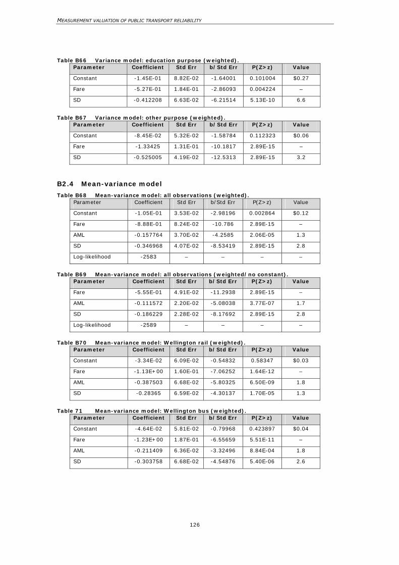
MEASUREMENT VALUATION OF PUBLIC TRANSPORT RELIABILITY
126
Table B66 Variance model: education purpose (weighted). Parameter Coefficient Std Err b/Std Err P(Z>z) Value
Constant -1.45E-01 8.82E-02 -1.64001 0.101004 $0.27
Fare -5.27E-01 1.84E-01 -2.86093 0.004224 –
SD -0.412208 6.63E-02 -6.21514 5.13E-10 6.6
Table B67 Variance model: other purpose (weighted).
Parameter Coefficient Std Err b/Std Err P(Z>z) Value
Constant -8.45E-02 5.32E-02 -1.58784 0.112323 $0.06
Fare -1.33425 1.31E-01 -10.1817 2.89E-15 –
SD -0.525005 4.19E-02 -12.5313 2.89E-15 3.2
B2.4 Mean-variance model
Table B68 Mean-variance model: all observations (weighted). Parameter Coefficient Std Err b/Std Err P(Z>z) Value
Constant -1.05E-01 3.53E-02 -2.98196 0.002864 $0.12
Fare -8.88E-01 8.24E-02 -10.786 2.89E-15 –
AML -0.157764 3.70E-02 -4.2585 2.06E-05 1.3
SD -0.346968 4.07E-02 -8.53419 2.89E-15 2.8
Log-likelihood -2583 – – – –
Table B69 Mean-variance model: all observations (weighted/no constant).
Parameter Coefficient Std Err b/Std Err P(Z>z) Value
Fare -5.55E-01 4.91E-02 -11.2938 2.89E-15 –
AML -0.111572 2.20E-02 -5.08038 3.77E-07 1.7
SD -0.186229 2.28E-02 -8.17692 2.89E-15 2.8
Log-likelihood -2589 – – – –
Table B70 Mean-variance model: Wellington rail (weighted).
Parameter Coefficient Std Err b/Std Err P(Z>z) Value
Constant -3.34E-02 6.09E-02 -0.54832 0.58347 $0.03
Fare -1.13E+00 1.60E-01 -7.06252 1.64E-12 –
AML -0.387503 6.68E-02 -5.80325 6.50E-09 1.8
SD -0.28365 6.59E-02 -4.30137 1.70E-05 1.3
Table 71 Mean-variance model: Wellington bus (weighted).
Parameter Coefficient Std Err b/Std Err P(Z>z) Value
Constant -4.64E-02 5.81E-02 -0.79968 0.423897 $0.04
Fare -1.23E+00 1.87E-01 -6.55659 5.51E-11 –
AML -0.211409 6.36E-02 -3.32496 8.84E-04 1.8
SD -0.303758 6.68E-02 -4.54876 5.40E-06 2.6
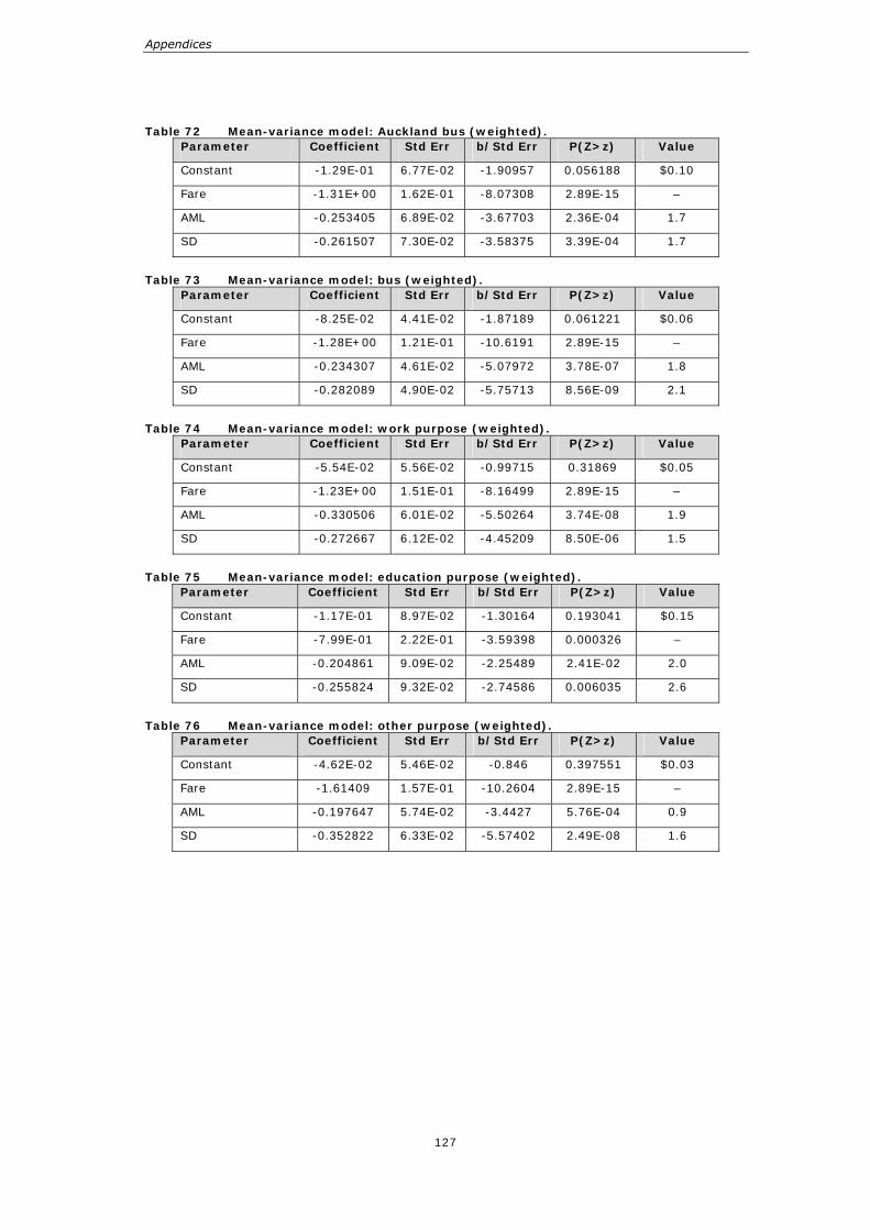
Appendices
127
Table 72 Mean-variance model: Auckland bus (weighted). Parameter Coefficient Std Err b/Std Err P(Z>z) Value
Constant -1.29E-01 6.77E-02 -1.90957 0.056188 $0.10
Fare -1.31E+00 1.62E-01 -8.07308 2.89E-15 –
AML -0.253405 6.89E-02 -3.67703 2.36E-04 1.7
SD -0.261507 7.30E-02 -3.58375 3.39E-04 1.7
Table 73 Mean-variance model: bus (weighted).
Parameter Coefficient Std Err b/Std Err P(Z>z) Value
Constant -8.25E-02 4.41E-02 -1.87189 0.061221 $0.06
Fare -1.28E+00 1.21E-01 -10.6191 2.89E-15 –
AML -0.234307 4.61E-02 -5.07972 3.78E-07 1.8
SD -0.282089 4.90E-02 -5.75713 8.56E-09 2.1
Table 74 Mean-variance model: work purpose (weighted).
Parameter Coefficient Std Err b/Std Err P(Z>z) Value
Constant -5.54E-02 5.56E-02 -0.99715 0.31869 $0.05
Fare -1.23E+00 1.51E-01 -8.16499 2.89E-15 –
AML -0.330506 6.01E-02 -5.50264 3.74E-08 1.9
SD -0.272667 6.12E-02 -4.45209 8.50E-06 1.5
Table 75 Mean-variance model: education purpose (weighted).
Parameter Coefficient Std Err b/Std Err P(Z>z) Value
Constant -1.17E-01 8.97E-02 -1.30164 0.193041 $0.15
Fare -7.99E-01 2.22E-01 -3.59398 0.000326 –
AML -0.204861 9.09E-02 -2.25489 2.41E-02 2.0
SD -0.255824 9.32E-02 -2.74586 0.006035 2.6
Table 76 Mean-variance model: other purpose (weighted).
Parameter Coefficient Std Err b/Std Err P(Z>z) Value
Constant -4.62E-02 5.46E-02 -0.846 0.397551 $0.03
Fare -1.61409 1.57E-01 -10.2604 2.89E-15 –
AML -0.197647 5.74E-02 -3.4427 5.76E-04 0.9
SD -0.352822 6.33E-02 -5.57402 2.49E-08 1.6

MEASUREMENT VALUATION OF PUBLIC TRANSPORT RELIABILITY
128
Measurement Valuation of Public Transport Reliability
Land Transport New Zealand Research Report 339