Embed Size (px)
Citation preview

C S A S
Canadian Science Advisory Secretariat
S C C S
Secrétariat canadien de consultation scientifique
* This series documents the scientific basis for the evaluation of fisheries resources in Canada. As such, it addresses the issues of the day in the time frames required and the documents it contains are not intended as definitive statements on the subjects addressed but rather as progress reports on ongoing investigations.
* La présente série documente les bases scientifiques des évaluations des ressources halieutiques du Canada. Elle traite des problèmes courants selon les échéanciers dictés. Les documents qu’elle contient ne doivent pas être considérés comme des énoncés définitifs sur les sujets traités, mais plutôt comme des rapports d’étape sur les études en cours.
Research documents are produced in the official language in which they are provided to the Secretariat. This document is available on the Internet at:
Les documents de recherche sont publiés dans la langue officielle utilisée dans le manuscrit envoyé au Secrétariat. Ce document est disponible sur l’Internet à:
http://www.dfo-mpo.gc.ca/csas/
ISSN 1499-3848 (Printed / Imprimé) © Her Majesty the Queen in Right of Canada, 2004
© Sa majesté la Reine, Chef du Canada, 2004
Habitat-based production goals for coho salmon in Fisheries and Oceans Statistical Area 3
Objectifs de production axés sur l’habitat pour le saumon coho dans le secteur statistique 3 de Pêches et Océans Canada
R.C. Bocking1 and D. Peacock2
1LGL Limited Environmental Research Associates 9768 Second Street
Sidney, B.C. V8L 3Y8
2Fisheries and Oceans Canada 417- 2nd Avenue West
Prince Rupert, B.C. V8J 1G8
Research Document 2004/129 Document de recherche 2004/129 Not to be cited without Permission of the authors
Ne pas citer sans autorisation des auteurs


Page i
TABLE OF CONTENTS LIST OF TABLES ......................................................................................................................... iii LIST OF FIGURES ........................................................................................................................iv LIST OF APPENDICES ..................................................................................................................v ACKNOWLEDGMENTS ..............................................................................................................vi ABSTRACT.................................................................................................................................. vii RÉSUMÉ ..................................................................................................................................... viii INTRODUCTION .......................................................................................................................... 1
Physical Habitats Limiting Coho Production ..................................................................... 3 Predicting Smolt Abundance from Physical Habitat .......................................................... 4 Study Area........................................................................................................................... 5 Current Management of Area 3 Coho ................................................................................. 6
AREA 3 COHO PRODUCTION MODEL .................................................................................. 10 DATA SOURCES AND MODEL INPUTS................................................................................. 11
Coho Distributions ............................................................................................................ 11 Accessible Stream Length................................................................................................. 12
Gradient ................................................................................................................. 13 Stream Order......................................................................................................... 13
Mean Smolt Yield ............................................................................................................. 14 Model 1 ................................................................................................................. 14 Model 2 ................................................................................................................. 16
Required number of Spawners .......................................................................................... 16 Fecundity............................................................................................................... 17 Freshwater Survival .............................................................................................. 18
Sensitivity Analyses .......................................................................................................... 18 MODEL RESULTS ...................................................................................................................... 19
Distribution of Nass Coho Habitat.................................................................................... 19 Accessible Stream Length................................................................................................. 19 Mean Smolt Yield ............................................................................................................. 19
Model 1 ................................................................................................................. 19 Model 2 ................................................................................................................. 22
Predicted Smolt Production .............................................................................................. 22 Predicted Spawner Requirements ..................................................................................... 26
SENSITIVITY ANALYSES ........................................................................................................ 28 Accessible Stream Length Determinations ....................................................................... 28 Freshwater Survival .......................................................................................................... 30
DISCUSSION............................................................................................................................... 32 Accessible Stream Length................................................................................................. 32 Effect of Map Scale ........................................................................................................... 33 Limits to Smolt Production............................................................................................... 33 Required Number of Spawners......................................................................................... 34 Comparison to Indicator Stocks ........................................................................................ 36

Page ii
Comparison to Other Area 3 Escapements ....................................................................... 39 Predicting Total Adult Returns and Harvest Rates ........................................................... 41
Conclusions ................................................................................................................................... 42 LITERATURE CITED ................................................................................................................. 44 APPENDICES .............................................................................................................................. 51

Page iii
LIST OF TABLES Table 1. Area 3 average coho escapement, 1950 to 1999 (DFO, Prince Rupert). ..........................8 Table 2. Sex ratio of coho spawners observed at the Zolzap Creek counting fence, 1998-
2002 (from Baxter 2003; Baxter and Stephens 2002, 2002a, 2002b; and Baxter et al. 2001). ..............................................................................................................................17
Table 3. Egg-to-smolt survivals for Zolzap Creek coho, 1992-1998 broods (data from Baxter et al. 2001).......................................................................................................................18
Table 4. Analysis of covariance sum of squares (SS), degrees of freedom (df) and hypotheses tests...............................................................................................................21
Table 5. Adjusted least square means by geographic group. ........................................................21 Table 6. Model 1 predicted coho smolt output by Area 3 regions for gradient less than 8%
and B parameter = 2, using region-wide regression. Prediction equation is ln (smolt yield) = 7.879 + 0.839*ln (length). .................................................................................24
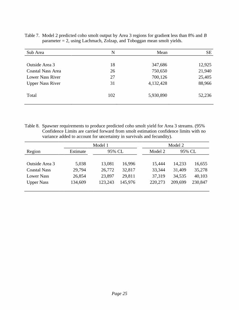
Table 7. Model 2 predicted coho smolt output by Area 3 regions for gradient less than 8% and B parameter = 2, using Lachmach, Zolzap, and Toboggan mean smolt yields........25
Table 8. Spawner requirements to produce predicted coho smolt yield for Area 3 streams. (95% Confidence Limits are carried forward from smolt estimation confidence limits with no variance added to account for uncertainty in survivals and fecundity). ..25
Table 9. Comparison of the total length of stream habitat available to coho in Statistical Area 3 using 100% slope for different lengths of stream as a gradient barrier. ......................29
Table 10. Estimated accessible length (m) over a range of gradient limits and stream order values (B). Italicized numbers are percent difference for gradient <2% / B=1 and gradient <8% / B=3. ........................................................................................................30
Table 11. Regression parameters required for Model 1 predictions when Zolzap and Lachmach were excluded from the region-wide dataset.................................................37
Table 12. Comparison of model results to recent decadel average smolt and spawner abundances and age-specific Ricker and Hockey Stick (Break Point Regression) models at Zolzap and Lachmach creeks. ........................................................................38
Table 13. Comparison of the required number of spawners for maximum smolt production (Smax) using various smolts per spawner estimates; Model 1 and 2 (survival estimates), Zolzap Hockey Stick model, Bradford et al. (2000) and Shaul et al. (2003). .............................................................................................................................40
Table 14. Comparison of model predictions for spawner abundance with AUC escapement estimates for Statistical Area 3 streams. .........................................................................40
Table 15. Required number of spawners and total return for Area 3 coho assuming different marine survival rates. ......................................................................................................43

Page iv
LIST OF FIGURES Figure 1. Map of Statistical Area 3 and coho streams. ...................................................................7 Figure 2. Schematic drawing of how stream order was used to determine accessible length
using different values of B (see equation 1). Bold areas indicate streams included in the analyses. Numbers indicated stream order. .........................................................14
Figure 3. Distribution of coho habitat as measured by accessible stream length less than 8% gradient and B = 2 for stream order equation (1) within Statistical Area 3...................20
Figure 4. Smolt yield as a function of stream length (km) by geographic group. .........................21 Figure 5. Smolt yield as a function of stream length (km) by significantly different
geographic groups. ........................................................................................................22 Figure 6. Smolt yield per kilometre for Lachmach Creek coho, by smolt year............................23 Figure 7. Smolt yield per kilometre for Zolzap Creek coho, by smolt year. ................................23 Figure 8. Smolt yield per kilometre for Toboggan Creek coho, by smolt year. ...........................24 Figure 9. Comparison of predicted smolt yield estimates for sub-regions in Area 3 using the
two different smolt yield models. ..................................................................................26 Figure 10. 95% confidence intervals for the prediction of smolt yield from accessible stream
length for Statistical Area 3. ..........................................................................................27 Figure 11. Estimated spawning requirements to produce predicted smolt yield in Statistical
Area 3. ...........................................................................................................................28 Figure 12. Sensitivity of the predicted spawner requirements to stream gradient and the
included stream network (order) as defined by B and using Model 1. ..........................31 Figure 13. Sensitivity of the predicted spawner requirements to freshwater survival estimates
using Model 1. ...............................................................................................................32 Figure 14. Daily discharge for four Nass River streams...............................................................35 Figure 15. Age-specific Ricker and Hockey Stick recruitment relationships for Zolzap Creek
coho smolts, 1992-1998 brood years. ............................................................................38

Page v
LIST OF APPENDICES Appendix A Watershed area, Mean Annual Discharge (MAD), stream order and accessible
length for Area 3 coho salmon streams................................................................................. 52 Appendix B Mean annual yield of coho smolts and accessible stream length data from
Bradford et al. (1997)............................................................................................................ 57 Appendix C Smolt yield estimates for Area 3 coho streams using 2 different models............. 59 Appendix D Estimate of the required number of coho spawners assuming Model 1 smolt
production (regional database).............................................................................................. 63 Appendix E Estimate of the required number of coho spawners assuming Model 2 smolt
production (local indicators). ................................................................................................ 68 Appendix F Estimation of total coho return and allowable harvest rates for assumed survival
rates. ............................................................................................................................... 73

Page vi
ACKNOWLEDGMENTS
We would like to acknowledge the contribution of several people to the development of this
model. Peter Wainwright, Robin Tamasi, Lucia Ferreira, Karen Truman, and Tony Mochizuki of
LGL all participated in the development of the GIS components of the model to calculate
accessibility from TRIM data. Mansell and Kimi Griffin of the Nisga’a Lisims Government also
assisted with the GIS calculations for the Coastal Nass Area streams. Bill Gazey conducted
statistical analyses for predicted smolt output. The support for this project by Nisga’a Lisims
Government, particularly Harry Nyce, is greatly appreciated. We also thank Michael Bradford
for providing the region wide dataset of smolt yields and for reviewing the manuscript. Thanks
also to Chuck Parken for reviewing the manuscript and to Joel Sawada for reviewing the
manuscript and assisting with the gathering of data for Lachmach, Toboggan and Alaskan coho
streams.

Page vii
ABSTRACT
Smolt productive capacity and the number of spawners that are required in order to fully seed the
available habitat and produce the maximum number coho smolts (Smax) were estimated for 102
coho streams in Statistical Area 3 using a habitat-based model. Stream length accessible to coho
salmon was determined from terrain resource inventory maps (TRIM) using GIS. Stream order,
gradient and known barriers were used to define the accessible length of stream. The number of
smolts per kilometre was derived using two models. The first used a log- linear predictive
regression of smolt yield and stream length for Alaskan and British Columbia streams. The
second used recent decadal smolt yield and stream length for three northern British Columbia
coho indicator streams (Lachmach, Zolzap, and Toboggan). Estimates of smolt productive
capacity and required spawner numbers were stratified into four geographic regions of Statistical
Area 3; Outer Coastal Area, Outer Nass Area, Lower Nass Area, and Nass River Area. The
predicted smolt yield from both models for Zolzap Creek was comparable to maximum smolt
yield from Ricker and Hockey Stock smolt recruitment relations. However, the estimated
required number of spawners to seed the available habitat in Zolzap Creek, and for all streams in
general was highly variable and depended on the assumed values of egg-to-smolt survival and
the number of smolts produced per spawner.

Page viii
RÉSUMÉ
La capacité de production des smolts et le nombre de géniteurs nécessaires pour ensemencer
complètement l’habitat disponible et pour produire un maximum de smolts de coho (Smax) ont été
estimés au moyen d’un modèle fondé sur l’habitat pour 102 cours d’eau à saumon coho dans le
secteur statistique 3. La longueur des cours d’eau accessible au saumon coho a été déterminée à
partir de cartes d’inventaire des ressources sur le terrain (terrain resource inventory maps
(TRIM)) dressées à l’aide d’un SIG. L’ordre, la pente et les obstacles connus des cours d’eau ont
été utilisés pour établir la longueur accessible au saumon. Le nombre de smolts par kilomètre a
été obtenu à l’aide de deux modèles : le premier était une régression prévisionnelle log- linéaire
du nombre de smolts produits dans les cours d’eau de l’Alaska et de la Colombie-Britannique et
de la longueur de ces cours d’eau; le deuxième à utilisé des données décennales récentes sur la
production de smolts dans trois cours d’eau indicateurs à saumon coho du nord de la C.-B.
(Lachmach, Zolzap et Toboggan) et sur la longueur de ces cours d’eau. Les estimations de la
capacité de production des smolts et du nombre de géniteurs nécessaires ont été classées selon
quatre régions géographiques du secteur statistique 3 : zone côtière extérieure, zone extérieure de
la rivière Nass, la zone du cours inférieur de la rivière Nass et la zone de la rivière Nass. Les
prévisions de la production de smolts dans le ruisseau Zolzap obtenues à l’aide des deux modèles
étaient comparables à la production maximale de smolts obtenue à l’aide des modèles de
recrutement de Ricker et de type « bâton de hockey ». Cependant, l’estimation du nombre de
géniteurs requis pour ensemencer l’habitat disponible dans le ruisseau Zolzap, et dans l’ensemble
des cours d’eau en général, était très variable et dépendait des valeurs présumées du taux de
survie de l’œuf au smolt et du nombre de smolts produits par géniteur.

Page 1
INTRODUCTION
The need to establish escapement goals based on stock-specific productive capacity is
fundamental to wild stock conservation and sustainability of coho salmon (Oncorhyncus kisutch)
fisheries in British Columbia. Canada’s draft Wild Salmon Policy states that target and limit
reference points will be determined for each salmon conservation unit based on estimates of
productive capacity (Fisheries and Oceans Canada 1998). Other jurisdictions that have recently
developed new policies regarding biological escapement goals or reference points include
Oregon, Washington and Alaska.
In Alaska, the state constitution mandates the Alaska Department of Fish and Game (ADF&G) to
manage fishery resources on the sustained yield principle (ADF&G 2001), requiring
establishment of escapement goals. Escapement goals or reference points are to be defined on
the basis of maximum sustained yield (MSY) with uncertainties explicitly stated.
In Washington State, the Department of Fish and Wildlife developed the Joint Wild Salmon
Policy (WDFW 1997). The WDFW spawning escapement policy states “escapement rates,
levels or ranges shall be designated to achieve MSY and will account for all relevant factors
including current abundance and survival rates, habitat capacity and quality, environmental
variation, management precision, and uncertainty and ecosystem interactions.” Still others have
recommended that escapement goals need to explicitly account for freshwater productivity
requirements such as nutrients from spawning carcasses (Cederholm et al. 2000). In Oregon,
estimates of carrying capacity are needed by fishery managers to implement the Oregon Wild
Fish Management Policy (ODFW 1992).
Each of these policies infer the need to develop salmon escapement goals or reference points
based on some measure of the ability of the stream (and marine) ecosystem to produce salmon.
However, estimating the productive capacity using conventional stock assessment techniques
(e.g., stock recruitment analysis) for each of the numerous coho stocks within a given
management area is a costly endeavour and greatly beyond the fiscal capability of Fisheries and
Oceans Canada. As well, the inherent difficulties in obtaining direct estimates of juvenile coho
production, catch estimates and spawner abundance on a stock-specific basis preclude the use of

Page 2
a stock recruit approach to estimate productive capacity for coho salmon. Hence, for virtually all
coho streams in British Columbia, there remains uncertainty regarding the appropriate
escapement goals for coho salmon. Moreover, stock recruitment analysis, a proposed method to
calculate the required number of spawners for coho in Statistical Area 3, would produce
unreliable estimates as a result of the high variability typically associated with spawner-recruit
data.
The establishment of regional or area-specific aggregate escapement goals for coho salmon is a
more realistic goal and is also in keeping with the management methods currently used for the
many mixed-stock coho fisheries in British Columbia. For example, Nisga’a entitlements to Nass
Area coho are based on a fixed percentage (8%) of the total return to Canada (TRC) for the Nass
Area aggregate, not specific stocks. Another example is Fraser River coho which are managed
to a single exploitation rate across all major stocks (Fisheries and Oceans Canada 2003). As
stock identification techniques for coho improve and are implemented inseason, harvest rates
may be targeted towards smaller stock groupings than currently possible.
An alternative to spawner-recruit relationships for determining productive capacity for coho is
habitat capacity modelling. Numerous authors have investigated relationships between fish
abundance in streams (number of spawners, smolt yield, fry density, etc.) and physical habitat
variables (e.g., Baranski 1989, Reeves et al. 1989, Holtby et al. 1990, Marshall and Britton 1990,
Jowett 1992, Nickelson et al. 1992, Bradford et al. 1997, Rosenfeld et al. 2000, Pess et al. 2002).
Faush et al. (1988) reviewed 99 models that predict the abundance of stream fish from habitat
variables. Water temperature, flow, depth, velocity, water quality, food availability, channel
characteristics, and watershed characteristics have all been considered in models (Jowett 1992).
These multi-variate models require intensive amounts of data for specific habitat characteristics
and may or may not be suitable beyond specific species, streams or geographic regions. For the
majority of the nearly 2,600 spawning populations of coho salmon in British Columbia (Slaney
et al. 1996), these data simply do not exist and would be too costly to collect.
One approach suggested by several authors (Holtby et al. 1990, Marshall and Britton 1990,
Bradford et al. 1997, Nickelson 1998, and Bocking et al. 2001) has been to quantify the amount
of freshwater rearing habitat that limits freshwater production within a stream or watershed and

Page 3
then predict fry or smolt yield from the habitat parameter. This approach assumes that the
average number of coho juveniles produced from a stream is an appropriate measure of a
stream’s “average” production potential or capacity (Marshall and Britton 1990, Bradford et al.
1997). Burns (1971) defined stream carrying capacity as: “the greatest weight of fishes that a
stream can naturally support during the period of least available habitat. It should be considered
a mean value around which populations fluctuate.” Carrying capacity in terms of juvenile
salmon production can only be achieved when a stream is adequately seeded with spawners.
The general belief is that the majority of coho production is derived from smolts (stream type) of
varying freshwater age (1-3 years in freshwater) (Mason 1975, Crone and Bond 1976). It is also
believed, however, that coho fry (ocean type) that leave their natal stream can also contribute, in
part, to total production by successfully rearing in neighbouring streams or estuarine
environments (Tschaplinksi 1987, Irvine and Johnston 1992). The contribution of this life-
history strategy is also inferred from discrepancies in the proportion of smolts coded-wire tagged
at exodus from the natal stream and the proportion of returning adults coded-wire tagged (e.g.
Baxter 2003, black, French, coldwater, etc.).
While numerous studies have documented the downstream movement and presumed emigration
of coho fry from the freshwater environment, few have quantified the contribution of this life-
history component of the population to total adult return. Bradford et al. 2000 suggested that fry
migrants could contribute significantly to total production if there are significant amounts of
suitable habitat in non natal areas where they are able to rear to smolt stage before entering the
marine environment. However, until quantitative studies are conducted to document the
contribution of fry to total adult return, it is appropriate to assume that the majority of coho
production in terms of adult returns is derived from stream type coho.
Physical Habitats Limiting Coho Production
Freshwater habitat quantity and quality determines the number of coho salmon smolts that a
stream can produce, typically referred to as carrying capacity of the stream. The limiting habitat
of a stream is that which is required to support a particular life stage but is in shortest supply.
For coho salmon, five freshwater life stages are typically recognized: 1) spawning and
incubation; 2) spring fry; 3) summer parr; 4) winter pre-smolts; and 5) smolts. Most coho

Page 4
populations smolt after one year in freshwater, but some portion of some populations can spend
up to two or three years before smolting.
When the habitat needed during a particular life stage is in short supply, a bottleneck is created
and the population suffers density-dependent mortality (Reeves et al. 1989). The most common
limiting seasons for coho salmon are late summer or winter and correspond to sustained periods
of low flows. Low stream flows can reduce available habitat to coho primarily by:
1. Narrowing the stream channel;
2. Reducing the number of pools and off channel areas;
3. Reducing the size and depth of pools and off channel areas; and
4. Reducing nutrient inputs to the stream by isolating watered areas from riparian
vegetation.
This reduction in habitat available can occur during late summer at which time the recruitment of
winter pre-smolts would be limited, or during winter at which time the recruitment to smolts
would be limited.
Solazzi et al. (2000) found that improving overwintering habitat for coho salmon parr and smolts
in Oregon streams resulted in a significant gain in productivity. These overwintering areas tend
to be in the lower reaches of streams where deep water pool habitat with cover and off channel
habitat is typically more abundant.
Predicting Smolt Abundance from Physical Habitat
Studies have shown that carrying capacity of a stream is related to physical attributes of the
stream (Marshall and Britton 1990). For example, Burns (1971) found that stream surface area
provided the best correlation with absolute biomass (all species) for seven northern California
streams. Chapman (1965) found similarity in coho densities among Oregon streams on a per unit
area basis. Mason and Chapman (1965) found coho production in Oregon to be most strongly
correlated with stream area. Lister (1968) found little difference in coho smolt yield per unit of
stream length in five British Columbia streams and concluded that 2,484 smolts per kilometre
was a useful biostandard for determining yield. Interestingly, Mason (1974) found that coho fry

Page 5
biomass could be increased substantially by augmenting the food supply with daily feedings of
euphausiids. However, smolt yield did not increase beyond expected natural levels.
Bradford et al. (1997) examined the relationship between mean smolt abundance and physical
habitat features from a database of 474 annual estimates of smolt abundance from 86 streams in
western North America. They found that only stream length and to a lesser extent latitude was
useful in predicting mean smolt abundance. Mean coho salmon smolt abundance was strongly
correlated with stream length (R2 = 0.70, Bradford et al. 1997). Marshall and Britton (1990)
found that both stream length and useable area were good predictors of mean smolt abundance
for 24 streams in the Pacific Northwest. Holtby et al. (1990) and Nickelson (1998) obtained
similar results with their datasets. Rosenfield et al. (2000) also found no decline in coho
abundance per linear kilometre of stream for 119 observations in British Columbia, which is
consistent with the observations of Bradford et al. (1997) that coho smolt production is a simple
linear function of stream length.
The approach of Bradford et al. (1997) assumes that the representative datasets in the model
contain sufficient years of data to approximate mean smolt abundance, at least for the period
covered by the data set. They may or may not represent periods of high smolt production, low
smolt production, or average smolt production. Nevertheless, they are the best estimates
available for smolt production from the various streams.
Using known or literature values of survival, coho smolt production estimates can then be used
to derive estimates of the required spawners to fully seed the available habitat and yield
maximum smolt production or capacity. It is this number of spawners required to maximize
smolt capacity production (Smax) that the models developed in this paper are attempting to
predict. Note that the model does not account for potential production arising from ocean-type
coho that might emigrate from freshwater systems in their first year of life, rear in non-natal
areas and still contribute to resulting adult returns.
Study Area
The study area for this work includes all of Fisheries and Oceans Statistical Area 3. The
southern boundary of Statistical Area 3 stretches from Dundas Island across Green Island to Port

Page 6
Simpson (Figure 1). Area 3 includes all Canadian waters north of this boundary, including
Observatory Inlet, Portland Inlet, Pearce Canal, and the Nass River.
Statistical Area 3 encompasses two ecoprovinces (Coastal Mountains and Sub-Boreal Interior)
and contains six biogeoclimatic zones: Alpine Tundra, Sub-Boreal Spruce, Engelmann Spruce-
Subalpine Fir, Interior Cedar-Hemlock, Mountain Hemlock, and Coastal Western Hemlock
(Meidinger and Pojar 1991).
There are a total of 102 known coho streams within Area 3 (Appendix A). Forty-four of these
are in coastal areas and fifty-eight are within the Nass River drainage. Coho escapements vary
significantly among all streams. Escapement data for the region are generally poor with not all
coho-bearing streams represented in the Fisheries and Oceans database and only two systems
having what could be considered rigorous counts (Meziadin River and Zolzap Creek; Table 1).
Additional estimates have been obtained for several streams using Area-Under-The-Curve
methods since 2000.
Current Management of Area 3 Coho
Area 3 coho are harvested in mixed-stock commercial, recreation, and First Nation fisheries.
Fisheries and Oceans Canada manages these fisheries to a maximum 15% Canadian exploitation
on aggregate North and Central coast coho stocks. Alaskan fisheries have typically harvested
between 20% and 40% of Area 3 coho stocks for a combined US and Canada harvest rate of
between 35% and 55%. As well, the Joint Fisheries Management Committee (JFMC)1 for the
Nisga’a Final Agreement is tasked with ensuring that Nisga’a entitlements as mandated by the
Final Agreement are achieved.
To deliver Nisga’a entitlements as per the Nisga’a Final Agreement and to optimize fishing
benefits for all Canadians has required that methods be developed to estimate the total harvest
and escapement of Area 3 coho as well as the establishment of escapement reference points. In
2000, indicator stocks were established to provide annual escapement estimates in the Coastal
1The Joint Fisheries Management Committee is a tripartite committee consisting of representatives of Nisga’a Lisims Government, the government of Canada, and the government of British Columbia.

Page 7
Figure 1. Map of Statistical Area 3 and coho streams.

Page 8
Table 1. Area 3 average coho escapement, 1950 to 1999 (DFO, Prince Rupert). Maximum
SUBAREA STREAM NAME 1950-59 1960-69 1970-79 1980-89 1990-99 Recorded
PORTLAND CANAL BEAR RIVER 975 3,333 2,219 2,071 625 7500PORTLAND CANAL BELLE BAY CREEK - - - 11 - 100PORTLAND CANAL DOGFISH BAY CREEK 30 - 69 63 52 500PORTLAND CANAL DONAHUE CREEK - - - - - - PORTLAND CANAL GEORGIE RIVER - 3,475 817 - - 12000PORTLAND CANAL RAINNY CREEK - - 83 350 88 500PORTLAND CANAL ROBERSON CREEK - 82 63 - - 400OBSERVATORY INLET CASCADE CREEK - - - - - - OBSERVATORY INLET ILLIANCE RIVER 1,422 150 165 550 375 3500OBSERVATORY INLET KITSAULT RIVER* 516 1,080 1,270 1,157 - 3000OBSERVATORY INLET KSHWAN RIVER 513 - - 544 - 2000OBSERVATORY INLET OLH CREEK - - - 25 - 100OBSERVATORY INLET SALMON COVE CREEK - - - 21 - 100OBSERVATORY INLET STAGOO CREEK - - 89 171 - 600OBSERVATORY INLET WILAUKS CREEK - - - 406 - 3000NASS RIVER ANLIYEN CREEK - - 220 363 - 700NASS RIVER ANSEDAGAN CREEK - 153 141 214 30 750NASS RIVER BOWSER RIVER & LAKE - - - - - - NASS RIVER BROWN BEAR CREEK - - 45 129 - 350NASS RIVER CHAMBERS CREEK - - - 113 107 320NASS RIVER CRANBERRY RIVER - 1,200 3,167 2,213 333 6000NASS RIVER DAMDOCHAX RIVER & LAKE - - 170 638 - 1000NASS RIVER DISKANGIEG CREEK - 75 586 600 - 1800NASS RIVER GINGIT CREEK - 344 307 78 50 750NASS RIVER GINLULAK CREEK - 1,050 795 855 467 3500NASS RIVER GITZYON CREEK 44 239 81 30 0 750NASS RIVER IKNOUK RIVER - - - 1,419 500 5000NASS RIVER ISHKHEENICKH RIVER 550 5,125 2,175 1,838 - 7500NASS RIVER KINCOLITH RIVER 381 - 300 1,780 1,500 5000NASS RIVER KINSKUTCH RIVER - - 17 27 - 50NASS RIVER KITEEN RIVER - 965 779 192 - 3500NASS RIVER KSEDIN CREEK - 159 92 68 90 400NASS RIVER KWINAGEESE RIVER - - 629 1,257 - 5000NASS RIVER KWINYARH CREEK - - 46 129 - 300NASS RIVER KWINYIAK RIVER - 933 342 269 100 3500NASS RIVER MCKNIGHT CREEK - - 112 268 65 1000NASS RIVER MEZIADIN RIVER & LAKE - 750 2,256 2,725 2,308 7500NASS RIVER NASS MAINSTEM - - 111 767 - 1000NASS RIVER OWEEGIE CREEK & LAKE - - 213 417 6 1000NASS RIVER QUILGAUW CREEK - - 41 36 - 200NASS RIVER SEASKINNISH CREEK 559 1,808 738 280 15 3500NASS RIVER SNOWBANK CREEK - - 45 275 - 700NASS RIVER TCHITIN RIVER - - 35 50 250 500NASS RIVER TEIGEN CREEK - - - 17 - 50NASS RIVER TSEAX RIVER 2,173 5,525 5,756 4,600 1,000 15000NASS RIVER TSEAX SLOUGH - - - 525 417 2000NASS RIVER VAN DYKE CREEK - - 15 64 - 150NASS RIVER VETTER CREEK & SLOUGH - - 281 18 - 2500NASS RIVER WEGILADAP CREEK - - 30 38 - 100NASS RIVER WILYAYANOOTH CREEK - - - 101 - 500NASS RIVER ZOLZAP CREEK 35 544 347 583 1,043 2438NASS RIVER ZOLZAP SLOUGH - - 131 358 - 600
Mean

Page 9
Table 1 (continued).
MaximumSUBAREA STREAM NAME 1950-59 1960-69 1970-79 1980-89 1990-99 Recorded
PORTLAND INLET KHUTZEYMATEEN RIVER 1,245 544 1,064 3,970 4,350 10000PORTLAND INLET KWINAMASS RIVER 935 7,025 4,444 3,605 2,600 20000PORTLAND INLET LIZARD CREEK - - - - - - PORTLAND INLET MANZANITA COVE CREEK - - 29 - - 200PORTLAND INLET TSAMPANAKNOK BAY CREEK - - - 2 - 20WORK CHANNEL ENSHESHESE RIVER 408 - 525 1,220 1,850 3500WORK CHANNEL LACHMACH RIVER - 289 250 527 1,010 2500WORK CHANNEL LEVERSON LAKE SYSTEM 490 188 325 13 - 1500WORK CHANNEL TOON RIVER 416 683 669 89 - 2500COASTAL AMERICAN BAY CREEK - - - 1 - 12COASTAL BRUNDIGE CREEK - - - 12 - 50COASTAL SANDY BAY CREEK - - - 3 - 20COASTAL STUMAUN CREEK - 75 - 3 - 750COASTAL TRACY CREEK 75 - - - - 75COASTAL TURK CREEK 75 - 200 - - 200
SUBAREA TOTAL: PORTLAND CANAL 1,005 6,533 2,190 1,848 306 19500SUBAREA TOTAL: OBSERVATORY INLET 2,103 1,230 1,515 2,171 300 10000SUBAREA TOTAL: NASS RIVER 3,368 16,540 17,188 20,054 5,565 36725SUBAREA TOTAL: PORTLAND INLET 2,180 7,515 4,765 7,577 5,650 20400SUBAREA TOTAL: WORK CHANNEL 1,230 783 1,300 1,762 2,860 5000SUBAREA TOTAL: COASTAL 23 75 20 12 - 750AREA 3 TOTAL 9,908 32,675 26,978 33,424 14,681 81925
Mean
and Lower Nass areas, including the continuation of enumeration programs at Zolzap Creek and
Lachmach Creek; while mark-recapture estimates were refined for the Upper Nass aggregate.
The mark-recapture estimate for Upper Nass Area serves as the escapement estimate for that
aggregate of coho stocks while a “scaling” approach is used for estimating the total return to
Canada for Coastal and Lower Nass Area coho. Annual escapements are derived by expanding
escapement estimates from indicator stocks in the Coastal Nass Area and the Lower Nass Area in
proportion to system specific and total area estimates of the number of spawners required to
maximize smolt production (Smax). This “scaling” approach has also been proposed by others.
Shaul et al. (2003) suggested that average smolt production could be used as the best estimate of
system capability (excluding low escapement years) and that these productivity estimates from
full indicator stocks can be scaled to habitat capability estimates for the stock aggregate to
generate an overall escapement goal.
A habitat-based approach to quantifying the productive capacity for Area 3 coho production was
determined to be the most appropriate approach to establishing escapement reference points at
this time. The habitat-based approach to deriving these system specific productivity estimates

Page 10
and total area spawner requirements are described in this paper as the Area 3 Coho Production
Model.
AREA 3 COHO PRODUCTION MODEL
The Area 3 Coho Production Model is a habitat-based model that predicts maximum smolt
abundance for each stream and the number of spawners that is required to produce the maximum
smolt abundance (Smax), using the length of stream available for coho rearing as the predictor
variable. The model first calculates the total length of stream that is accessible coho for 102
watersheds in Statistical Area 3 using stream gradient, known barriers and stream order (Strahler
1957). A relationship between smolt yield and stream length was then developed using two
different approaches. The first approach used a log- linear model to predict smolt yield from
stream length using smolt production data from Southeast Alaska and British Columbia (circa
1950-present). In the second approach, recent ten-year mean smolt production measures for
three northern BC coho indicator stocks (Lachmach, Zolzap, Toboggan) were used and the
average smolts produced per kilometre of stream for these systems was applied to Area 3 coho
streams on a sub-regional basis.
Using estimates of survival by life stage, the model then calculated the number of spawners that
would be required to produce the estimated number of smolts. Model estimates of smolt
production and the required number of spawners were compared to empirical data collected for a
subset of the 102 watersheds that were included in the model. Inter-annual variability in smolt
production was incorporated into both models and hence into the smolt predictions for Area 3
streams.
The coho production model carries with it the critical assumption that stream length of stream
orders greater than 2 (at 1:20,000 scale) is a valid surrogate measure for the limiting habitat
available to coho pre-smolts and ultimately limits the amount of smolts produced by the system.
This assumption is supported by the fact that there is a downstream movement of fry during fall
and winter freshets to occupy lower areas of streams as pre-smolts (Cederholm and Reid 1987).
A portion of coho fry migrating downstream may also exit the freshwater environment either

Page 11
passively due to environmental clues (e.g. flooding, freeze-up) or actively due to territorial
displacement (Bilby and Bisson 1987, Hartman et al. 1981). The number of smolts emigrating
from the stream after one or more years of freshwater residency is the refore assumed to be a
function of the number of fry that survive to become parr in their first year of freshwater
residency. The limiting factor for maximizing steelhead production is often cited as the
availability of suitable habitat at the parr stage (Ptolemy et al. 2004).
The Area 3 Coho Production Model also assumes then that this production bottleneck occurring
during the parr-smolt stage of freshwater life for coho is primarily a function of available
suitable riverine habitat for yearling coho (hereafter referred to as pre-smolts). To the authors’
knowledge, there have been no attempts to quantify any relationship between the amount of late
summer or winter rearing habitat available to coho pre-smolts and stream length. However,
Sharma and Hilborn (2001) did find that lower valley slopes, lower stream gradients, and pool
and pond densities were correlated with higher smolt densities.
DATA SOURCES AND MODEL INPUTS
Coho Distributions
The Fisheries and Oceans catalogue of salmon streams and spawning escapements (Hancock and
Marshall 1984) and the Stream Summary Catalogue (DFO 1991) were used to develop a list of
all coho-bearing streams in Statistical Area 3 (Appendix A). Streams for which the topography
suggested no reason why coho would not be present were also included. For the most part, these
were watersheds in the upper Nass River drainage where information on coho distributions was
extremely limited or nonexistent.
Van Schubert (1999) conducted fish reconnaissance surveys in areas of the Nass watershed
upstream of the confluence of Damdochax Creek in late September of 1998. No anadromous
salmon with the possible exception of steelhead were identified in any of the sites sampled.
Based on these results, the entire Nass drainage upstream of Damdochax Creek was considered
to have zero coho potent ial, even though small amounts of each tributary appear to be accessible

Page 12
to anadromous salmon (Van Schubert 1999). Barriers to anadromous fish are present near the
mouth of each of these systems.
Streams were categorized based on the sub-region within Area 3 into which their watersheds
emptied. The four sub-regions were: Outer Coastal Area 3, Coastal Nass Area, Lower Nass
River, and Upper Nass River. The Upper Nass River above Damdochax was treated as a separate
tributary and the Kiteen River that empties into the Cranberry was also treated as a separate
tributary system. As well, the Bell-Irving River was stratified into upper, middle, and lower
sections. The mainstem of the Nass River, below Damdochax was also not included as parr-
smolt rearing habitat in the model.
All known coho producing streams from Fisheries and Oceans records were included in the
analysis. These watersheds were primarily of 3rd order or greater on 1:20,000 Digital Terrain
Resource Information Management (TRIM) mapping (Ministry of Sustainable Resource
Management). Although only stream order 2, Manzanita Creek was also included in the analysis
because of noted good abundances of coho.
Accessible Stream Length
The length of stream within a tributary accessible to coho is restricted by barriers to migration,
gradient, discharge, water quality (dissolved oxygen, turbidity, temperature), as well as
evolutionary distribution factors. Waterfalls, debris jams, and excessive water velocities may
impede fish access into otherwise suitable habitat. However, assessing whether or not a natural
obstruction (e.g., falls, cascade, and chute) is a barrier is not easy. Falls that are insurmountable
at one time of the year may be passed at other times under different flows (Bjornn and Reiser
1991). Powers and Orsborn (1985) reported that the ability of salmonids to pass over barriers is
dependent on the swimming velocity of adult fish, the horizontal and vertical distances to be
jumped, and the angle to the top of the barrier. The pool depth to height ratio is also important
(Stuart 1962). Bjorn and Reiser (1991) determined a maximum jumping height for coho of 2.2
m under optimal conditions.
The Area 3 Coho Model used a height estimate of 2.0 m for an obstruction to be considered a
barrier to coho. The model also considered that a point along the stream course where gradient
Page 13
exceeded 100% (45o) for longer than 10 metres would also be a barrier to coho migration.
Sensitivity analyses were performed on the “run” or length of the stream segment from 1 m to 10
m for a slope of 45o.
All available information on barriers within the Nass drainage was used to restrict coho use in
systems. The sources of information on barriers included FISS (1991a, b), Aquatic Biophysical
Maps (MOE 1977), unpublished information from the Ministry of Water, Land and Air
Protection, and data gathered through Watershed Restoration Program studies (NTC 1994-98)
and Fish Inventory Projects (NTC 1998a-h, Van Schubert 1999, Saimoto and Saimoto 1998).
The total accessible stream length within each Nass tributary was calculated from digital TRIM
files (1:20,000 scale) using ARCINFO and stratified according to gradient and stream order.
Where lakes were present within the network of accessible stream, the length of centre lines
connecting accessible lake tributaries to the lake outlet was included in the total length
calculation. This had the net effect of including a portion of the lake something less than the
perimeter as suitable habitat for coho parr.
Gradient
Pess et al. (2002) found that coho spawner abundance was correlated with stream gradient in the
Snohomish River, Washington. Coho have been reported to occur in stream segments with
gradients ranging from one to ten percent, with the greatest densities occurring in the lower
gradients. Higher gradient areas are dominated by larger substrate and lack the pool habitat
favoured by coho for rearing (Bisson et al. 1982). The Area 3 Coho Model assumed that stream
gradients over 8% were not utilized by coho parr or pre-smolts for rearing and that all gradients
below 8% had similar density of coho. ARCINFO and a gradient analysis program were used to
calculate the accessible length of stream within each watershed. For sensitivity analyses,
accessible area was determined for upper gradient limits of 2%, 4%, 6% and 8%.
Stream Order
Stream orders were determined using a method developed by Horton (1945) and later modified
by Strahler (1957) and were determined from the BC TRIM digital mapping (1:20000 scale).
The analysis allowed for the summation of accessible length for stream orders greater than 3 and
determination of the proportional contribution of 3rd order or larger streams.

Page 14
The Area 3 Coho Model also assumed that coho would not occupy stream habitats more than two
stream orders distance from the main stem. For example, for large streams of order 7, the
minimum stream order included for that watershed was 5. Figure 2 schematically illustrates this
algorithm.
Orderused = orderwshd – B equation (1)
4 4 4 4
5 4 5 43 3
4 45 3 1 5 3 1
2 22 1 2 1
6 1 6 11 1
Mouth Mouth
B = 2 B = 3
Figure 2. Schematic drawing of how stream order was used to determine accessible length using different values of B (see equation 1). Bold areas indicate streams included in the analyses. Numbers indicated stream order.
Mean Smolt Yield
Model 1
The first model for smolt yield used a large geographic data set to determine the smolt yield per
kilometre of stream. Annual yield of coho smolts and the associated accessible stream length
were compiled for all Alaska, BC, Washington and Oregon streams from Bradford et al. (1997)
(Appendix B). The mean coho smolt yield was calculated for streams with three or more annual
estimates. Streams were then classified, a priori, into the following three geographical groups:

Page 15
(1) Alaska and Northern BC; (2) Southern BC; and (3) Washington and Oregon. This grouping
was based on evidence of lower productivity (smolts produced per unit length) for southern
streams. Alaska and Northern BC streams were combined to maintain a reasonable sample size
of 9 streams (albeit still a small number). The Keogh River on northern Vancouver Island was
the most northerly of the Southern BC streams (Appendix B).
The effects of geographical groups and stream length on yield of smolts were examined using
analysis of covariance following Milliken and Johnson (2002). The smolt yield and stream
length were logarithmic transformed to obtain homogeneous variance residuals. The analysis
consisted of the application of two covariance models. The first was as follows:
ln{smolt yield} = constant + group + ln{stream length} + group*ln{stream length} equation (2)
where group is a categorical variable coded to the geographical groups defined above. The
interaction term (group*ln{stream length}) was tested for significance. This interaction term
represents the slopes of the regression lines of ln{yield} on ln{stream length}. Since the
interaction term was not statistically significant (see Results below), a simpler second model
without the interaction term was employed:
ln{smolt yield} = constant + group + ln{stream length} equation (3)
The group term now represents the relative mean ln{smolt yield} for parallel regression lines at
any given stream length value (e.g., the intercept). The group term was tested for significance
and the orthogonal contrasts (the group term partitioned into two single degree of freedom
contrasts) were calculated. The two contrasts considered were:
1. Alaska and Northern BC (group 1) combined with Southern BC (group 2) versus
Washington and Oregon (group 3); and
2. Alaska and Northern BC (group 1) versus Southern BC (group 2).
A predictive regression model for all Nass region streams was then constructed combining all
groups not significantly different from Alaska and Northern BC (group 1). Predictions of log-

Page 16
transformed smolt yield and the associated variance were then made given the stream length
using the well known predictive regression functions (e.g., Draper and Smith 1981). The
arithmetic expectation and variance for smolt yield was next calculated assuming a log-normal
distribution using:
{ }2/ˆ+ˆexp=][ 2sµYE equation (4)
and
{ } { }( )1ˆexpˆ+ˆ2exp=)( 22 -ssµYVar equation (5)
where µ is the mean and 2s is the variance of the logged transformed predictions (Johnson and
Kotz 1970). Assuming the stream predictions are independent, the mean for the area is the sum
of the mean of the component streams. Thus, the predicted means were summed for each
watershed in the Nass region. The variance terms for each component stream can be similarly
summed to get area-wide variance values. The summed mean and variance estimates can be
regarded as normally distributed according to the central limit theorem.
Model 2
The second model for smolt yield used the mean (1991-2000) annual smolt yield per kilometre
for Lachmach, Zolzap, and Toboggan applied to Area 3 streams. Lachmach smolt yield was
applied to all coastal areas of Area 3; Zolzap smolt yield was applied to all lower Nass
tributaries; and Toboggan Creek smolt yield was applied to all Upper Nass systems. Variability
around these estimates was estimated using the observed variability for Lachmach, Zolzap and
Toboggan.
Required number of Spawners
Determining the number of spawners required to produce a given number of smolts involved
back calculating from the smolt estimate to spawners using fecundity and survival estimates.
Limited data for coho sex ratios are available for Statistical Area 3 streams. The average sex
ratio of adult coho passing the counting weir at Zolzap Creek from 1998-2000 was 1.03 (M/F;
Table 2). Sex ratio for the purposes of calculating the number of spawners required in the model
was, therefore, assumed to be 1.0.

Page 17
Table 2. Sex ratio of coho spawners observed at the Zolzap Creek counting fence, 1998-2002
(from Baxter 2003; Baxter and Stephens 2002, 2002a, 2002b; and Baxter et al. 2001).
Year Males Females Ratio (M/F) 1998 517 437 1.18 1999 713 574 1.24 2000 188 217 0.87 2001 1,076 816 1.32 2002 753 1111 0.68
All Years 3,247 3,155 1.03
Fecundity
The required number of spawners to fully seed the available habitat was determined for each
stream using estimates of fecundity. The number of eggs per female for Outside Area 3 coho
was estimated using data from Lachmach River; for the Coastal Nass Area data from Kincolith
River was used; and for the Lower and Upper Nass Area data from Zolzap Creek and Tseax
River were used. Direct measures of fecundity were only available for Kincolith River and
Tseax River. For Lachmach River, length data from the 1989 brood were used to calculate
fecundity as:
Eggs per Female = 1.8933 (log(FL)) – 1.8612 equation (6)
where FL = female fork length at maturity.
The same equation was used for Zolzap Creek to convert female length data from 1996-99 to an
estimate of fecundity. The fecundity estimate for Lachmach was 2,906 eggs per female based on
an average length of 649 mm for the 1989 brood (Joel Sawada, DFO, pers. comm.). Fecundity
estimates for Kincolith coho, obtained from hatchery broodstock collections in 1995 and 1996
(Richard Alexander, pers. comm.), averaged 3,736 (n = 64). Recognizing inter-stream variability
in fecundity and to be conservative, a fecundity of 3,000 eggs per female was used in the model
for all Outer Coastal Area 3 and Coastal Nass Area streams.
The fecundity estimate for Zolzap Creek coho ranged from 2,461 to 2,931 for brood years 1996-
1999 with a mean of 2,629. The average fecundity for Tseax River coho (1993-94) was 2,500

Page 18
eggs per female. Therefore, for simplicity, a fecundity of 2,500 eggs per female was used in the
model for all Lower Nass Area and Upper Nass Area streams.
Freshwater Survival
Freshwater survival estimates for coho salmon are only available for Zolzap Creek in the Lower
Nass Area. Therefore, an egg-to-fry survival of 19.8% and a fry-to-smolt survival of 7.6%
(Bradford 1995) were used to calculate the number of spawners required to produce the
estimated smolt yield for each stream and area. This translates to an overall egg-to-smolt
survival of 1.5%. This survival is similar to survival observed at Zolzap Creek (1.6%) for the
1992 to 1998 broods (Table 3).
Table 3. Egg-to-smolt survivals for Zolzap Creek coho, 1992-1998 broods (data from Baxter et al. 2001).
Brood Year Spawners Females Eggs Smolts
Recruited Egg-to Smolt
Survival
1992 1,561 781 2,341,500 17,306 0.7% 1993 1,048 524 1,572,000 13,396 0.9% 1994 2,536 1,268 3,804,000 23,116 0.6% 1995 908 454 1,362,000 19,669 1.4% 1996 1,039 520 1,558,500 17,701 1.1% 1997 470 235 705,000 10,641 1.5% 1998 967 484 1,450,500 41,292 2.8% Mean 1,218 609 1,827,643 20,446 1.3%
Sensitivity Analyses
Sensitivity analyses were performed on a number of model parameters to explore the sensitivity
of predicted smolt yield and required spawner numbers to those parameters. The parameters
tested were gradient barrier criteria, stream order (B value), gradient criteria for rearing, egg-to-
fry survival, and fry-to-smolt survival. Fecundity estimates were not evaluated in the sensitivity
analyses.

Page 19
MODEL RESULTS
Distribution of Nass Coho Habitat
Figure 3 shows the distribution of Area 3 coho habitat as determined by the model. Coho habitat
in Area 3 is widely distributed among the 102 streams. There are a few major producers in each
area (e.g., Khutzemateen, Bear, Kwinamass, Ishkeenickh, Bell Irving, Kwinageese and
Cranberry).
Accessible Stream Length
Estimated accessible lengths for all Area 3 streams are provided in Figure 3 and Appendix A.
All model estimates of accessible stream length were based on an upper gradient limit of 8% and
a B of 2 for the stream order determination.
Mean Smolt Yield
Model 1
Figure 4 provides the regression plots of smolt yield versus stream length for the three
geographical groups. The results of the covariance analysis and orthogonal contrasts are listed in
Table 4. Note that the regression slopes can be viewed as equal (P=0.324) and the simpler
covariance model (parallel lines) indicates that the groups are significantly different (P<0.001).
The orthogonal contrasts indicate that Washington and Oregon are substantially different than
the other two groups combined (P<0.001) while there is little difference between the Alaska and
Northern BC (group 1) and Southern (group 2) groups (P=0.427).
Table 5 lists the adjusted least square log-transformed means (at the mean stream length) of the
geographical groups.
The regression plots with the significantly different groups (Alaska and BC combined) are
provided in Figure 5. The predictive regression used for the Nass region was then:
ln(smolt yield} = 7.87868 + 0.83923 * ln{stream length} equation (7)
R2 = 0.70

Page 20
Outside Area 3
0
5000
10000
15000
20000
25000
30000
35000
Am
eric
an B
ay Bill
Boat
Har
bour
Bru
ndig
e
Cow
Lag
oon
Ensh
eshe
se
Fort
une
Khu
tzey
mat
een
Lach
mac
h
Leve
rson
Mar
ion
Sand
y B
ay
Stum
aun
Toon
Trac
y
Tsam
pana
knok
Whi
tley
Poin
t
Leng
th o
f Str
eam
(m)
Coastal Nass Area
0
10000
20000
30000
40000
50000
60000
70000
Bea
rB
ell B
ayB
onan
zaCa
scad
eC
ham
bers
Dog
fish
Bay
Don
ahue
Geo
rgie
Illia
nce
Isaa
cK
inco
lith
Kits
ault
Ksh
wan
Kw
inam
ass
Lim
eLi
zard
Olh
Pear
ceR
ober
son
Rod
gers
Rou
ndy
Salm
on C
ove
Scow
bank
Stag
ooTa
uwW
ilauk
s
Leng
th o
f St
ream
(m
)
Lower Nass River
0
10000
20000
30000
40000
50000
60000
70000
80000
Anl
iyen
Ans
edeg
anA
nudo
lB
urto
nC
hem
ainu
kCu
gila
dap
Dis
kani
eqG
ingi
etl
Gin
lula
kG
ish
Gis
wat
zG
itwin
ksih
lkw
Ikno
ukIn
ieth
Ishk
eeni
ckh
Kea
zoah
Kse
mam
aith
Kw
inia
kK
win
aryh
Mon
kley
Qui
lgau
wSe
aski
nnis
hTs
eax
Weg
iliad
apW
elda
Wily
ayaa
noot
hZo
lzap
Leng
th o
f St
ream
(m
)
Upper Nass River
0
20000
40000
60000
80000
100000
120000
140000
160000
Upp
er B
ell I
rvin
gM
iddl
e B
ell-
Low
er B
ell-
Irvi
ngB
owse
rC
ranb
erry
Dam
doch
axH
odde
rK
insk
utch
Kite
enK
onig
usK
otsi
nta
Ksh
adin
Kw
inag
eese
Kw
inat
ahl
Mez
iadi
nM
uska
boo
Pano
ram
aPa
wSa
lada
mis
Sally
sout
Snas
kiso
otSa
nyam
Shum
alTa
ftTa
ylor
Tchi
tinTi
egen
Trea
tyU
pper
Nas
sV
ileW
hite
Leng
th o
f Str
eam
(m)
Figure 3. Distribution of coho habitat as measured by accessible stream length less than 8% gradient and B = 2 for stream order equation (1) within Statistical Area 3.

Page 21
-2 -1 0 1 2 3 4 5 6Ln(Stream Length)
5
6
7
8
9
10
11
12
13Ln
( Sm
oltY
ield
)
Washington and OregonSouthern BCAlaska and Northern BC
Figure 4. Smolt yield as a function of stream length (km) by geographic group.
Table 4. Analysis of covariance sum of squares (SS), degrees of freedom (df) and hypotheses tests.
Component SS(Test) df(Test) SS(Error) df(Error) F Probability Slopes 1.78 2 37.12 48 1.15 0.3241 Groups 14.04 2 38.90 50 9.02 0.0005 1&2 vrs 3 13.54 1 38.90 50 17.41 0.0001 1 vrs 2 0.50 1 38.90 50 0.64 0.4266
Table 5. Adjusted least square means by geographic group.
Group N Adj. Mean Std. Error Alaska and Northern BC 9 9.702 0.294 Southern BC 19 9.416 0.203 Washington and Oregon 26 8.501 0.173

Page 22
-2 -1 0 1 2 3 4 5 6Ln(Stream Length)
5
6
7
8
9
10
11
12
13Ln
(Sm
oltY
ield
)
Washington and OregonAlaska and BC
Figure 5. Smolt yield as a function of stream length (km) by significantly different geographic groups.
Model 2
At the time of this study, annual smolt yields for Lachmach, Zolzap and Toboggan creeks were
available from the early 1990s to 2000 (Figure 6, Figure 7, and Figure 8). Means over the period
1990 to 2000 were 27,163 smolts for Lachmach, 29,833 for Zolzap and 50,724 for Toboggan. As
such, average smolt yields per kilometre were 2383, 3088, and 2892 for Lachmach, Zolzap and
Toboggan respectively. Mean smolt yield for Lachmach was applied to Outer Coastal Area 3 and
the Coastal Nass Area streams; mean smolt yield for Zolzap was applied to the Lower Nass Area
streams; and mean smolt yield for Toboggan was applied to Upper Nass Area streams.
Predicted Smolt Production
The predicted smolt production by stream for each of the two models is provided in Appendix C.
Area totals with standard deviations are summarized in Table 6 and Table 7 and displayed in Figure
9. Model 1 used region-wide estimates over a 40 year time period, while Model 2 used area-specific

Page 23
0
1000
2000
3000
4000
5000
6000
1990 1992 1994 1996 1998 2000 2002
Year
Smol
t Yie
ld p
er K
ilom
etre
Lachmach
Mean = 2383
SE = 303
Figure 6. Smolt yield per kilometre for Lachmach Creek coho, by smolt year.
0
1000
2000
3000
4000
5000
6000
1990 1992 1994 1996 1998 2000 2002
Year
Smol
t Yie
ld p
er K
ilom
etre
Zolzap
Mean =
SD = 533
Figure 7. Smolt yield per kilometre for Zolzap Creek coho, by smolt year.

Page 24
0
1000
2000
3000
4000
5000
6000
1990 1992 1994 1996 1998 2000 2002
Year
Smol
t Yie
ld p
er K
ilom
etre
Toboggan
Mean = 2892
SD = 360
Figure 8. Smolt yield per kilometre for Toboggan Creek coho, by smolt year.
Table 6. Model 1 predicted coho smolt output by Area 3 regions for gradient less than 8% and B parameter = 2, using region-wide regression. Prediction equation is ln (smolt yield) = 7.879 + 0.839*ln (length).
Sub Area N Mean SE Outside Area 3 18 339,441 20,940 Coastal Nass Area 26 672,516 33,118 Lower Nass River 27 505,125 27,053 Upper Nass River 31 2,532,001 104,704 Total 102 4,049,084 62,310
Page 25
Table 7. Model 2 predicted coho smolt output by Area 3 regions for gradient less than 8% and B parameter = 2, using Lachmach, Zolzap, and Toboggan mean smolt yields.
Sub Area N Mean SE Outside Area 3 18 347,686 12,925 Coastal Nass Area 26 750,650 21,940 Lower Nass River 27 700,126 25,405 Upper Nass River 31 4,132,428 88,966 Total 102 5,930,890 52,236
Table 8. Spawner requirements to produce predicted coho smolt yield for Area 3 streams. (95% Confidence Limits are carried forward from smolt estimation confidence limits with no variance added to account for uncertainty in survivals and fecundity).
Model 1 Model 2 Region Estimate 95% CL Model 2 95% CL Outside Area 3 5,038 13,081 16,996 15,444 14,233 16,655 Coastal Nass 29,794 26,772 32,817 33,344 31,409 35,278 Lower Nass 26,854 23,897 29,811 37,319 34,535 40,103 Upper Nass 134,609 123,243 145,976 220,273 209,699 230,847

Page 26
-
1,000,000
2,000,000
3,000,000
4,000,000
5,000,000
6,000,000
7,000,000
OutsideArea 3
CoastalNass
LowerNass
UpperNass
TotalArea 3
Pred
icte
d Sm
olt Y
ield
Model 1 Model 2
Figure 9. Comparison of predicted smolt yield estimates for sub-regions in Area 3 using the two different smolt yield models.
measures over a recent ten-year period. Model 2 estimates of smolt production were higher than for
Model 1, particularly for the Lower Nass and Upper Nass areas. 95% confidence intervals on the
area-specific estimates of smolt yield are shown in Figure 10.
Predicted Spawner Requirements
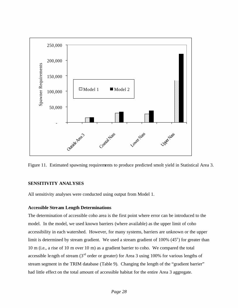
Figure 11 and Table 8 (see also Appendix D and Appendix E) show estimates of the number of
spawners required to produce the number of smolts calculated by the two models. As a result of
higher estimates smolt yields, Model 2 produced higher numbers of required spawners than Model 1,
particularly for the Lower and Upper Nass areas. Confidence limits on the predicted spawner
abundances are also shown in Table 8, but these do not include the considerable uncertainty
associated with the survival parameters used to back-calculate required spawners from the predicted
smolt yield.

Page 27
Outside Area 3
0
50000
100000
150000
200000
250000
300000
350000
400000
450000
Model 1 Model 2
Smol
t Yie
ld
Coastal Nass Area
0
100000
200000
300000
400000
500000
600000
700000
800000
900000
Model 1 Model 2
Smol
t Yie
ld
Lower Nass River
0
100000
200000
300000
400000
500000
600000
700000
800000
Model 1 Model 2
Smol
t Yie
ld
Upper Nass River
0
500000
1000000
1500000
2000000
2500000
3000000
3500000
4000000
4500000
Model 1 Model 2
Smol
t Yie
ld
Figure 10. 95% confidence intervals for the prediction of smolt yield from accessible stream length for Statistical Area 3.
Page 28
-
50,000
100,000
150,000
200,000
250,000
Outside
Area 3
Coastal
Nass
Lower N
ass
Upper N
ass
Spaw
ner R
equi
rem
ents
Model 1 Model 2
Figure 11. Estimated spawning requirements to produce predicted smolt yield in Statistical Area 3.
SENSITIVITY ANALYSES All sensitivity analyses were conducted using output from Model 1.
Accessible Stream Length Determinations
The determination of accessible coho area is the first point where error can be introduced to the
model. In the model, we used known barriers (where available) as the upper limit of coho
accessibility in each watershed. However, for many systems, barriers are unknown or the upper
limit is determined by stream gradient. We used a stream gradient of 100% (45o) for greater than
10 m (i.e., a rise of 10 m over 10 m) as a gradient barrier to coho. We compared the total
accessible length of stream (3rd order or greater) for Area 3 using 100% for various lengths of
stream segment in the TRIM database (Table 9). Changing the length of the “gradient barrier”
had little effect on the total amount of accessible habitat for the entire Area 3 aggregate.

Page 29
Reducing the gradient barrier length from 10 m to 1 m resulted in only a reduction of 0.67 % in
the total available length of stream for coho.
Table 9. Comparison of the total length of stream habitat available to coho in Statistical Area 3 using 100% slope for different lengths of stream as a gradient barrier.
Length of Stream Segment (km) 10 m 5 m 2 m 1 m 3rd Order and greater 3,898,080 3,898,080 3,897,620 3,872,160
% difference 0% 0.01% 0.67%
To test model sensitivity to the 8% gradient used as the upper limit of coho distribution (pres-
smolt rearing habitat) and the stream order algorithm used, the model was run using upper
gradient limits ranging from <2% to <8%. The model was also run using B parameters ranging
from 1 to 3 (see equation 1 and Figure 2). Note, that as B increases, the number of tributaries off
the mainstem included in the model increases, hence the length of useable stream habitat
increases. Similarly, decreasing the upper gradient limit for accessibility decreased the estimate
of accessible length.
The model was fairly robust over the range of gradient and B parameter tested and was more
sensitive to B than gradient (Figure 12). Errors in gradient and B had the most pronounced effect
on the predicted spawner requirements for the Upper Nass area where terrain relief was lowest.
Changing the upper gradient limit to 2% from 8% resulted in roughly a 25% decrease in the
estimate of accessible stream length for the B values tested (Table 10). The sensitivity to B was
more pronounced, particularly for the Upper Nass area where changing the B value for the
stream order network from 1 to 3 resulted in a 48-58% increase in the length of stream accessible
to coho and a significant change in the number spawners predicted.

Page 30
Table 10. Estimated accessible length (m) over a range of gradient limits and stream order values (B). Italicized numbers are percent difference for gradient <2% / B=1 and gradient <8% / B=3.
Area Gradient B 1 2 3 % Difference
<8% 134070 145920 173680 23% Outer Coastal Area 3 <6% 127940 139240 165060 22% <4% 118940 129580 152640 22% <2% 103270 113280 132700 22% % Difference 23% 22% 24% Coastal Nass <8% 223140 315040 355780 37% <6% 207800 296260 331630 37% <4% 191250 274820 304780 37% <2% 167400 242020 266800 37% % Difference 25% 23% 25% Lower Nass <8% 199290 226700 272430 27% <6% 191740 217650 257160 25% <4% 180960 203110 234270 23% <2% 155810 170690 190190 18% % Difference 22% 25% 30% Upper Nass <8% 888500 1428970 2098070 58% <6% 858210 1365800 1941570 56% <4% 815410 1263190 1722510 53% <2% 758440 1121380 1461120 48% % Difference 15% 22% 30%
Freshwater Survival
The model was also tested for sensitivity to the freshwater survival values that were used to
calculate the required number of spawners (19.8% egg-to-fry survival and 7.6% fry-to-smolt
survival). A range of egg-to-fry and fry-to-smolt survivals was tested. The model was most
sensitive to fry-to-smolt survival (Figure 13), particularly when it was decreased to less than 5%
resulting in significant positive error in the required spawners.

Page 31
Coastal Area 3
-50%
-30%
-10%
10%
30%
50%
70%
8% 6% 4% 2%Gradient
Pred
ictiv
e Er
ror i
n R
equi
red
Spaw
ners
B = 1 B = 2 B = 3
Coastal Nass Area
-50%
-30%
-10%
10%
30%
50%
70%
8% 6% 4% 2%Gradient
Pred
ictiv
e Er
ror i
n R
equi
red
Spaw
ners
B = 1 B = 2 B = 3
Lower Nass Area
-50%
-30%
-10%
10%
30%
50%
70%
8% 6% 4% 2%Gradient
Pred
ictiv
e Er
ror i
n R
equi
red
Spaw
ners
B = 1 B = 2 B = 3
Upper Nass Area
-50%
-30%
-10%
10%
30%
50%
70%
90%
8% 6% 4% 2%Gradient
Pred
ictiv
e Er
ror i
n R
equi
red
Spaw
ners
B = 1 B = 2 B = 3
Figure 12. Sensitivity of the predicted spawner requirement s to stream gradient and the included stream network (order) as defined by B and using Model 1.

Page 32
-100%
0%
100%
200%
300%
400%
500%
600%
700%
2.0% 5.0% 7.5% 10.0% 15.0%
Fry-to-Smolt Survival
Pred
ictiv
e Er
ror i
n R
equi
red
Spaw
ners 10% Egg-to-Fry Survival
15% Egg-to-Fry Survival
20% Egg-to-Fry Survival
25% Egg-to-Fry Survival
Figure 13. Sensitivity of the predicted spawner requirements to freshwater survival estimates using Model 1.
DISCUSSION
Identification of escapement targets is critical for management of coho salmon in Area 3 and
implementation of the Nisga’a Treaty which also requires an estimate of Total Return to Canada
(TRC) for the Nass Area each year. The Area 3 Coho Model described here is the first attempt at
defining escapement goals for coho in this area. The premise of correlation between smolt yield
and stream length is well supported in the literature and the use of the large geographic data set
for Model 1 ensures robustness across stream size and type.
Accessible Stream Length
Digital Terrain Resource Information Management (TRIM) maps at a 1:20,000 scale for
Statistical Area 3 were used for this model. TRIM maps are derived from air photo
interpretation and are considered to be accurate to within 10 m, 90% of the time (Brown et al.
Base case

Page 33
1996). However, tree vegetation makes capture of all waterways difficult from air photos. In an
examination of TRIM mapping with ground surveys, Brown et al. (1996) found that TRIM
delineated 80% of the natural channel length in basins with terrain relief. The percentage
delineated by TRIM in areas of low relief was 73%. The watersheds included in the Area 3 Coho
Model have significant terrain relief and TRIM likely captures the majority of the stream
network that is accessible to coho salmon.
Effect of Map Scale
Model 1 was derived using region-wide data for smolts/km for which stream length was derived
primarily from 1:50,000 or higher scale maps (M. Bradford, pers. comm.), with the exception of
Zolzap and Lachmach creeks (Area 3 streams). The stream lengths for Area 3 streams were
derived from 1:20,000 scale TRIM maps. Therefore, Model 1 may overestimate the smolt
capacity for Area 3 streams due to a mismatch of map scales. However, this would likely be
small for the Coastal Area and Lower Nass Area streams where topographic relief is quite high
and the accessible stream length determined from 1:50,000 scale versus 1:20,000 scale maps
would be similar. Map scale may be more of a concern for some Upper Nass Area streams
where relief is lower and additional tributaries (particularly 3rd order), with a significant amount
of available coho habitat, may be captured at 1:20,000 scale but not appear on 1:50,000 scale
mapping.
Limits to Smolt Production
Coho smolt production appears to be independent of the number of spawners except at low
spawner abundances (Bradford et al. 2000, Knight 1980, Holtby and Scrivener 1989). Nickelson
et al. (1992) concluded that coho salmon in Oregon are likely limited by the availability of
winter habitat (also Brown and Hartman 1988). Furthermore, several authors have documented
the downstream movement of coho juveniles from upper watershed areas to lower watershed
areas in the fall (Brown et al. 1999, Cederholm and Scarlett 1991). This movement is likely in
preparation for smolting and perhaps a response to habitat contraction due to drying or freezing.
It is these behaviours, which likely enable the prediction of smolt production from available
rearing habitat (e.g., stream length) in the higher order streams within a watershed.

Page 34
The Nass River and its watersheds are characterized by dramatic fluctuations in flow (Figure 14).
There are typically two low flow periods, late summer and winter. Freezing in winter also
reduces available habitat in some parts of the Nass watershed. The life stages of salmonids at
these critical times (fall fry, and pre-smolts) become the limiting stages to total smolt production.
During these times, available habitat to rearing salmonids is contracted and the mainstem and
primary tributaries account for a greater proportion of the available and useable habitat. It is this
interrelation between critical flow and available habitat that likely allows for stream length to be
a reasonable predictor of smolt production.
Required Number of Spawners
The applicability of Model 1 for predicting the number of spawners required to maximize smolt
production in Statistical Area 3 carries with it many assumptions. Perhaps foremost, the model
assumes that the historical mean smolt data used to derive the model is reflective of smolt
productive capacity for the geographic region included (BC and Alaska). Although this is
consistent with the thinking of previous researchers; namely that average smolt production is an
appropriate measure of capacity (Marshall and Britton 1990, Bradford et al. 1997, Burns 1971);
this assumption should be tested in future research. Similarly, the suitability of Model 2 as a
predictor of the required number of spawners to maximize smolt production in Statistical Area 3
depends on the recent decadel average smolt production for Zolzap, Lachmach, and Toboggan
being an appropriate measure of capacity for those systems.
Both models evaluated in this paper predict the required number of spawners for smolt
production. They ignore potential production from ocean-type coho that leave the freshwater
environment in their first year. For those Area 3 systems where ocean-type coho contribute to
total coho production measured by adult returns, the models would underestimate the required
number of spawners to maximize total production. Similarly, to the extent that coho from
adjacent streams rear in non-natal streams in the study area, there will be errors in the predicted
number of required spawners for those systems. There is very limited data for Statistical Area 3
coho streams to test either of these assumptions.

Page 35
Cranberry River (2000-02)
0
5
10
15
20
25
30
35
40
45
50
55
60
65
1-Jan 1-Apr 30-Jun 28-Sep 27-Dec
Dai
ly D
isch
arge
(m
3/s)
Diskangieq Creek (2001-02)
0
1
2
1-Jan 1-Apr 30-Jun 28-Sep 27-Dec
Dai
ly S
tage
(m3 /s
)
Tintina Creek (2001-02)
0
5
10
15
20
25
1-Jan 1-Apr 30-Jun 28-Sep 27-Dec
Dai
ly D
isch
arge
(m3/
s)
Kwinageese River (2001-02)
0
10
20
30
40
50
60
70
1-Jan 1-Apr 30-Jun 28-Sep 27-Dec
Dai
ly D
isch
arge
(m
3/s)
Figure 14. Daily discharge for four Nass River streams.

Page 36
A number of additional assumptions were made when determining the number of required
spawners to maximize smolt production. These include assumptions about freshwater survival,
which were shown to have a significant effect on the model predictions. Currently, freshwater
survival is only measured at Zolzap Creek. The addition of another coho indicator stock,
particularly for the Upper Nass, would greatly enhance understanding of coho production in the
Nass region.
Sex ratio was assumed to be one to one. If this is not the case for the majority of streams, then
the prediction of the required number of spawners could be biased. Egg retention and other
factors potentially limiting spawning success were also not factored into the model. If spawning
success is significantly less than 100%, then the required number of spawners would be under
predicted. The sensitivity of the model to assumptions about sex ratio, fecundity and spawning
success should be evaluated in the future.
Not withstanding the various assumptions and limitations of the models tested, we recommend in
the interim that estimates of the required number of spawners for Area 3 coho be based on the
results of Model 1 for smolt yield, and that the “average” survival rates from Bradford (1995) be
used. There may be considerable error in the predictions for some streams, but on an area basis,
the predictions are a major step toward improved fishery management capability for Area 3
coho, especially where escapement goals for coho do not currently exist. The results suggest that
appropriate escapement goals should be in the range of 15,000 spawners for Outer Coastal Area
3, 30,000 for the Coastal Nass Area, 26,000 for the Lower Nass Area, and 135,000 for the Upper
Nass Area. These spawner abundances would produce, on average, smolt yields in keeping with
regional estimates per kilometre for BC and Southeast Alaskan streams.
Comparison to Indicator Stocks
The performance of Model 1 was evaluated against recent average smolt production at Zolzap
Creek and Lachmach Creek (data from Baxter and Stephens 2002 and Holtby et al. 1999). A
“leave-one-out” analysis of Model 1 was conducted for this evaluation by systematically
omitting Zolzap and then Lachmach from the region-wide data set used in the development of
Model 1. Table 11 contains the regression parameters used for Model 1 in each case to predict
smolt production and spawner requirements for Zolzap and Lachmach.
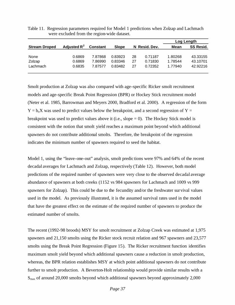
Page 37
Table 11. Regression parameters required for Model 1 predictions when Zolzap and Lachmach were excluded from the region-wide dataset.
Stream Droped Adjusted R2 Constant Slope N Resid. Dev. Mean SS Resid.
None 0.6869 7.87868 0.83923 28 0.71187 1.80268 43.33155Zolzap 0.6869 7.86990 0.83346 27 0.71830 1.78544 43.10701Lachmach 0.6835 7.87577 0.83482 27 0.72352 1.77940 42.92216
Log Length
Smolt production at Zolzap was also compared with age-specific Ricker smolt recruitment
models and age-specific Break Point Regression (BPR) or Hockey Stick recruitment model
(Neter et al. 1985, Barrowman and Meyers 2000, Bradford et al. 2000). A regression of the form
Y = boX was used to predict values below the breakpoint, and a second regression of Y =
breakpoint was used to predict values above it (i.e., slope = 0). The Hockey Stick model is
consistent with the notion that smolt yield reaches a maximum point beyond which additional
spawners do not contribute additional smolts. Therefore, the breakpoint of the regression
indicates the minimum number of spawners required to seed the habitat.
Model 1, using the “leave-one-out” analysis, smolt predic tions were 97% and 64% of the recent
decadal averages for Lachmach and Zolzap, respectively (Table 12). However, both model
predictions of the required number of spawners were very close to the observed decadal average
abundance of spawners at both creeks (1152 vs 984 spawners for Lachmach and 1009 vs 999
spawners for Zolzap). This could be due to the fecundity and/or the freshwater survival values
used in the model. As previously illustrated, it is the assumed survival rates used in the model
that have the greatest effect on the estimate of the required number of spawners to produce the
estimated number of smolts.
The recent (1992-98 broods) MSY for smolt recruitment at Zolzap Creek was estimated at 1,975
spawners and 21,150 smolts using the Ricker stock recruit relation and 967 spawners and 23,577
smolts using the Break Point Regression (Figure 15). The Ricker recruitment function identifies
maximum smolt yield beyond which additional spawners cause a reduction in smolt production,
whereas, the BPR relation establishes MSY at which point additional spawners do not contribute
further to smolt production. A Beverton-Holt relationship would provide similar results with a
Smax of around 20,000 smolts beyond which additional spawners beyond approximately 2,000

Page 38
Table 12. Comparison of model results to recent decadel average smolt and spawner abundances and age-specific Ricker and Hockey Stick (Break Point Regression) models at Zolzap and Lachmach creeks.
Model 11 Model 2 Decadel Average2
Ricker MSY3 Hockey Stick3
Lachmach smolts 26,350 27,091 27,163 Na NaLachmach spawners 1,152 1,203 984 Na NaZolzap smolts 18,977 24,120 29,833 21,150 23,577Zolzap spawners 1,009 1,286 999 1,975 967
1 Model 1 derived using "leave-one-out" analysis whereby Zolzap and Lachmach were excluded from region-wide data set when predicting respective smolts production.2 Smolt averages are for 1992-2001 smolt years and spawner abundances are for 1992-2000.3 Brood year data for stock recruit analyses are from 1992-97 for Zolzap (Baxter and Stephens 2002).
0
5,000
10,000
15,000
20,000
25,000
30,000
35,000
40,000
45,000
0 500 1,000 1,500 2,000 2,500 3,000 3,500 4,000
Brood Year Spawners
Rec
ruitm
ent o
f Sm
olts
'98 Brood
HS = 23,577 smolts / 967 spawners
Smax = 21,150 smolts /1,975 spawners
Model 1 = 18,977 smolts / 1,009 spawners
Figure 15. Age-specific Ricker and Hockey Stick recruitment relationships for Zolzap Creek coho smolts, 1992-1998 brood years.
Page 39
would contribute no further to production. The Lachmach recruitment data were not informative
enough to enable a Ricker or Hockey Stick model fit due to the absence of age-specific smolt
recruitment information.
Model 1 and the Hockey Stick model predicted very similar required spawner numbers providing
some validation to the notion, at least for Zolzap Creek, that the model is predicting the
maximum smolt production and the minimum number of coho spawner required, on average.
Both the model estimates of smolt and spawner requirements and the actual estimates for smolt
production and spawners at Zolzap and Lachmach are not without error. The actual smolt
estimates were derived at these systems (and Toboggan) using smolt fences (e.g. Baxter and
Stephens 2002). The decadel smolt estimates for these systems in Table 12 could be in error due
to non-natal rearing of coho within and/or outside these parent streams, and errors in counting.
For the purpose of comparing model predictions, however, these errors were assumed to be small
compared to inter-annual variability in the estimates (see Appendix B). Similarly, errors in
spawner estimates were assumed to be small compared to inter-annual variability (SD for Zolzap
= 550; SD for Lachmach = 300) as the recent spawner abundance estimates for Lachmach and
Zolzap were from weir counts and/or rigorous mark-recapture estimates.
Table 13 compares the model estimates of smolts per spawner with those reported for Zolzap
Creek using the Hockey Stick function (this paper), by Bradford et al. (2000) for 14 Washington
and southern BC coho streams, and by Shaul et al. (2003) for Southeast Alaskan streams. The
habitat model estimates of the required number of spawners are higher than what would be
predicted using estimates of smolts per spawner from the other sources, indicating that the
survival parameters used in this report may result in an overestimate of the required number of
spawners. However, the number of smolts per spawner was similar for the habitat models and
for the Zolzap Hockey Stick model indicating that, at least for the lower Nass and coastal areas,
the models may be appropriate.
Comparison to Other Area 3 Escapements
Fisheries and Oceans and Nisga’a Lisims Government have been monitoring escapements using
area-under-the-curve (AUC) techniques since 2000 for four Area 3 coho streams. As well, coho

Page 40
escapements to Meziadin River have been completely counted at a fishway since 2000. Table 14
compares the habitat model spawner predictions with recent escapement levels for these systems.
Table 13. Comparison of the required number of spawners for maximum smolt production (Smax) using various smolts per spawner estimates; Model 1 and 2 (survival estimates), Zolzap Hockey Stick model, Bradford et al. (2000) and Shaul et al. (2003).
Required Spawners
Model 1
Zolzap Hockey
Stick Bradford et
al. (2000) Shaul et al. (2002) Smolts per spawner: 19.6 24.5 42.5 30 60
From Model 1 Smolts Outside Area 3 15,038 13,855 7,987 11,315 5,657 Coastal Nass 29,794 27,450 15,824 22,417 11,209 Lower Nass 26,854 20,617 11,885 16,837 8,419 Upper Nass 134,609 103,347 59,576 84,400 42,200 Total Area 3 206,296 165,269 95,273 134,969 67,485
Model 2
Zolzap Hockey
Stick Bradford et
al. (2000) Shaul et al. (2002) Smolts per spawner: 19.4 24.5 42.5 30 60
From Model 2 Smolts Outside Area 3 15,444 14,191 8,181 11,590 5,795 Coastal Nass 33,344 30,639 17,662 25,022 12,511 Lower Nass 37,319 28,577 16,474 23,338 11,669 Upper Nass 220,273 168,671 97,234 137,748 68,874 Total Area 3 306,380 242,077 139,550 197,696 98,848
Table 14. Comparison of model predictions for spawner abundance with AUC escapement estimates for Statistical Area 3 streams.
AUC System Model 1 Model 2 2000-02 Range 2000-02
Mean Salmon Cove 620 565 219-986 573 Diskangieq 1,150 1,475 408-3,325 2,233 Ginlulak 914 1,123 339-1,965 1,180 Ansedegan 474 512 58-1,483 586 Meziadin 9,960 17,069 1,439-5,965 4,149 Upper Nass 134,609 220,273 72,000-168,000 109,000
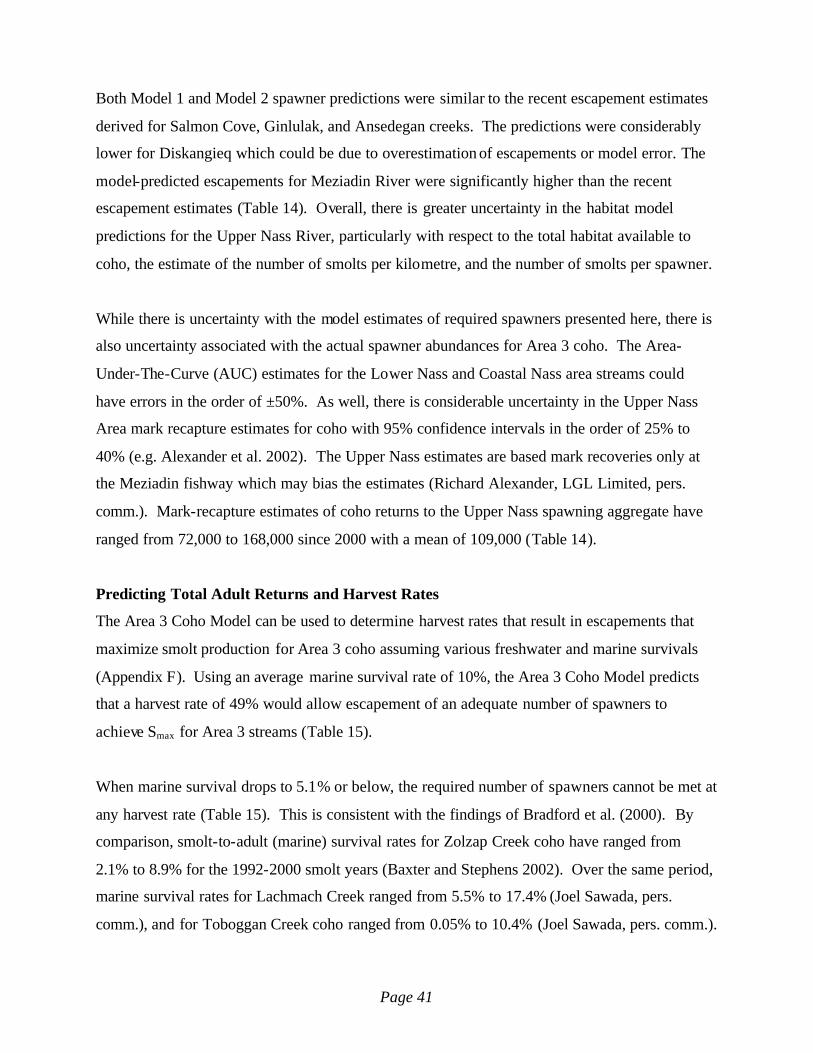
Page 41
Both Model 1 and Model 2 spawner predictions were similar to the recent escapement estimates
derived for Salmon Cove, Ginlulak, and Ansedegan creeks. The predictions were considerably
lower for Diskangieq which could be due to overestimation of escapements or model error. The
model-predicted escapements for Meziadin River were significantly higher than the recent
escapement estimates (Table 14). Overall, there is greater uncertainty in the habitat model
predictions for the Upper Nass River, particularly with respect to the total habitat available to
coho, the estimate of the number of smolts per kilometre, and the number of smolts per spawner.
While there is uncertainty with the model estimates of required spawners presented here, there is
also uncertainty associated with the actual spawner abundances for Area 3 coho. The Area-
Under-The-Curve (AUC) estimates for the Lower Nass and Coastal Nass area streams could
have errors in the order of ±50%. As well, there is considerable uncertainty in the Upper Nass
Area mark recapture estimates for coho with 95% confidence intervals in the order of 25% to
40% (e.g. Alexander et al. 2002). The Upper Nass estimates are based mark recoveries only at
the Meziadin fishway which may bias the estimates (Richard Alexander, LGL Limited, pers.
comm.). Mark-recapture estimates of coho returns to the Upper Nass spawning aggregate have
ranged from 72,000 to 168,000 since 2000 with a mean of 109,000 (Table 14).
Predicting Total Adult Returns and Harvest Rates
The Area 3 Coho Model can be used to determine harvest rates that result in escapements that
maximize smolt production for Area 3 coho assuming various freshwater and marine survivals
(Appendix F). Using an average marine survival rate of 10%, the Area 3 Coho Model predicts
that a harvest rate of 49% would allow escapement of an adequate number of spawners to
achieve Smax for Area 3 streams (Table 15).
When marine survival drops to 5.1% or below, the required number of spawners cannot be met at
any harvest rate (Table 15). This is consistent with the findings of Bradford et al. (2000). By
comparison, smolt-to-adult (marine) survival rates for Zolzap Creek coho have ranged from
2.1% to 8.9% for the 1992-2000 smolt years (Baxter and Stephens 2002). Over the same period,
marine survival rates for Lachmach Creek ranged from 5.5% to 17.4% (Joel Sawada, pers.
comm.), and for Toboggan Creek coho ranged from 0.05% to 10.4% (Joel Sawada, pers. comm.).

Page 42
CONCLUSIONS
We conclude that the area aggregate escapement requirements (goals) using Model 1 presented
in Table 8 currently represent the best estimates of the number of coho salmon spawners required
to produce the maximum smolt yields for Area 3 streams. Additional tests of model assumptions
and uncertainty as discussed should be performed in future iterations of model development and
refinement. As well, the dataset originally compiled by Bradford et al. (1997) and used to
develop Model 1 could perhaps be updated to include more recent years and additional streams
to improve the spatial and temporal representativeness of the model. A more critical review of
each stream’s suitability for input to the model should also be performed. This should include
recalculating accessibility to coho for these streams using the Area 3 Coho Production Model
algorithm for limiting coho distributions where barriers are not field-verified.
With respect to empirical studies to support the model, we recommend the continuation of
escapement estimation for indicator stocks in Area 3 as well as continued mark-recapture
estimation of escapement, stock-recruitment analyses, and ground truthing of accessible stream
lengths and suitable habitats. Overtime, additional information on known barriers to migration
should replace the GIS-based algorithm used to limit coho distribution in Area 3 streams.
Information on life-history strategies and population traits for Upper Nass Area coho populations
would also aid in determining the appropriateness of the model for these streams. The role of the
Nass mainstem in providing additional rearing habitat for Upper Nass Area coho (and perhaps
Lower Nass Area coho to some extent ) should also be investigated.

Page 43
Table 15. Required number of spawners and total return for Area 3 coho assuming different marine survival rates.
Required Total Return for Various Marine Survivals Area Spawners 2% 4% 5.10% 6% 8% 10% 12% 14%
Outer Coastal Area 3 15,038 6,789 13,578 17,312 20,366 27,155 33,944 40,733 47,522 Coastal Nass Area 29,794 13,450 26,901 34,298 40,351 53,801 67,252 80,702 94,152 Lower Nass Area 26,854 10,102 20,205 25,761 30,307 40,410 50,512 60,615 70,717 Upper Nass Area 134,609 50,640 101,280 129,132 151,920 202,560 253,200 303,840 354,480 Total 206,296 80,982 161,963 206,503 242,945 323,927 404,908 485,890 566,872 Percent of Required Spawners 39% 79% 100% 118% 157% 196% 236% 275% Allowable Harvest Rate 0% 15% 36% 49% 58% 64%
1 Harvest rate that would result in escapements that maximize smolt production

Page 44
LITERATURE CITED
Alaska Department of Fish and Game (ADF&G). 2001. Alaska’s conservation mandate.
http://www.state.ak.us/adfg/geninfo/hot/brochure.htm (Sept. 2001). Alexander, R.F., M.R. Link, and R.C. Bocking. 2002. The 2000 fishwheel project on the Nass
River, BC. Can. Manuscr. Rep. Fish. Aquat. Sci. 2626: 118 p. Baranski, C. 1989. Coho smolt production in ten Puget Sound streams. Wash. Dep. Fish. Tech.
Rep. 99: 29 p. Barrowman, N.J. and R.A. Myers. 2000. Still more spawner-recruitment curves: the hockey
stick and its generalizations. Can. J. Fish. Aquat. Sci. 57: 665-676. Baxter, B.E. 2003. Adult and juvenile coho salmon enumeration and coded-wire tag recovery
analysis for Zolzap Creek, BC. 2002. Can. Manuscr. Rep. Fish. Aquat. Sci. No. 2646: vii + 44 p.
Baxter, B.E. and C.Y. Stephens. 2002. Adult and juvenile coho salmon enumeration and coded-
wire tag recovery analysis for Zolzap Creek, BC. 2001. Can. Manuscr. Rep. Fish. Aquat. Sci. No. 2601: viii + 44 p.
Baxter, B.E. and C.Y. Stephens. 2002a. Adult and juvenile coho salmon enumeration and
coded-wire tag recovery analysis for Zolzap Creek, BC. 2000. Can. Manuscr. Rep. Fish. Aquat. Sci. No. 2598: viii + 44 p.
Baxter, B.E. and C.Y. Stephens. 2002b. Adult and juvenile coho salmon enumeration and
coded-wire tag recovery analysis for Zolzap Creek, BC. 1999. Can. Manuscr. Rep. Fish. Aquat. Sci. No. 2597: viii + 44 p.
Baxter, B.E., C.Y. Stephens and B.L. Nass. 2001. Adult and juvenile coho salmon enumeration
and coded-wire tag recovery analysis for Zolzap Creek, BC. 1998. Can. Manuscr. Rep. Fish. Aquat. Sci. No. 2566: viii + 44 p.
Baxter, B.E., C.Y. Stephens, and R.C. Bocking. 2002. Nisga’a catch monitoring program: 2001
Nisga’a fishery. Nisga’a Fisheries Report No. NF01-04. Bilby, R.E. and P.A. Bisson. 1987. Emigration and production of hatchery coho salmon
(Oncorhynchus kisutch) stocked in streams draining an old-growth and a clear-cut watershed. Can. J. Fish. Aquat. Sci. 44: 1397-1407.
Bisson, P.A., R.A. Nielsen, R.A. Palmason, and L.E. Gore. 1982. A system of naming habitat
types in small streams with examples of habitat utilization by salmonids during low stream flow. In Acquisition and utilization of aquatic habitat information. Edited by N.A. Armatrout. American Fisheries Society, Bethesda, MD. Pp. 62-73.

Page 45
Bjorn, T.C. and D.W. Reiser. 1991. Habitat requirements of salmonids in streams. American Fisheries Society Special Publication 19: 83-138.
Bocking, R.C., C.K. Parken, and D.Y. Atagi. 2001. Nass River steelhead habitat capability
production model and preliminary escapement goals. Unpublished report for Ministry of Water, Land and Air Protection, Smithers, British Columbia.
Bradford, M.J. 1995. Comparative review of Pacific salmon survival rates. Can. J. Fish. Aquat.
Sci. 52: 1327-1338. Bradford, M.J., G.C. Taylor and J.A. Allan. 1997. Empirical review of coho salmon smolt
abundance and the prediction of smolt production at the regional level. Trans. Am. Fish. Soc. 126: 49-64.
Bradford, M.J., R.A. Myers and J.R. Irvine. 2000. Reference points for coho salmon
(Oncorhynchus kisutch) harvest rates and escapement goals based on freshwater production. Can. J. Fish. Aquat. Sci. 57: 677-686.
Brown, T.G. and G.F. Hartman. 1988. Contribution of seasonally flooded lands and minor
tributaries to coho (Oncorhynchus kisutch) salmon smolt production in Carnation Creek, a small coastal stream in British Columbia. Trans. Am. Fish. Soc. 1217: 546-551.
Brown, T.G., L. Barton, and G. Langford. 1996. The use of a geographic information system to
evaluate terrain resource information management (TRIM) maps and to measure land use patterns for Black Creek, Vancouver Island. Can. Manuscr. Rep. Fish. Aquat. Sci. 2395: 34 p.
Brown, T.G., L. Barton, and G. Langford. 1999. Coho salmon habitat within Black Creek,
Vancouver Island. Can. Tech. Rep. Fish. Aquat. Sci. 2294: 75 p. Burns, J.W. 1971. The carrying capacity for juvenile salmonids in some northern California
streams. Calif. Fish and Game. Vol. 57 (1) : 44-57. Cederholm, C.J. and L.M. Reid. 1987. Impacts of forest management on coho salmon
(Oncorhynchus kisutch) populations of the Clearwater River, Washington: project summary, p. 373-398. In E.W. Salo and T.W. Cundy (ed.). Streamside Management: forestry and fisheries interactions. Contribution 57, College of Forest Resources, University of Washington, Seattle, WA.
Cederholm, C.J. and W.J. Scarlett. 1991. The beaded channel: a low-cost technique for
enhancing winter habitat of coho salmon. Amer. Fish. Soc. Symposium 10: 104-108. Cederholm, C.J., M.D. Kunze, T. Murota, and A Sibatani. 2000. Pacific salmon carcasses:
essential contributions of nutrients and energy for aquatic and terrestrial ecosystems. Fisheries 24, No. 10: 6-15.

Page 46
Chapman, D.W. 1965. Net production of juvenile coho salmon in three Oregon streams. Trans. Am. Fish. Soc. 94 (1): 40-52.
Crone, R.A. and C.E. Bond. 1976. Life history of coho salmon, Oncorhynchus kisutch, in Sashin
Creek, southeastern Alaska. Fish. Bull. U.S. 74: 897-923. DFO. 1991. Stream Summary Catalogue Subdistrict #3. Fish Habitat Inventory and Information
Program. North Coast Division, Fisheries Branch, Department of Fisheries and Oceans. Draper, N.R., and W. Smith. 1981. Applied Regression Analysis (Second Ed.). John Wiley and
Sons. 709p Faush, K.D., C.L. Hawkes, and M.G. Parsons. 1988. Models that predict standing crop of
stream fish from habitat variables: 1950-85. USDA For. Serv. Gen. Tech. Rep. PNW-GTR-213, Portland, OR. 52 p.
Fisheries and Oceans Canada. 1998. Draft Wild Salmon Policy. A new direction for Canada’s
Pacific Salmon Fisheries, policy paper, released for review October 1998. http://www-comm.pac.dfo-mpo.gc.ca/english/newdirections/default.htm (Sept. 2001).
FISS. 1991a. Fish Habitat Inventory and Information Program Stream Summary Catalogue:
Subdistrict #3A, Lower Nass. Department of Fisheries and Oceans. FISS. 1991b. Fish Habitat Inventory and Information Program Stream Summary Catalogue:
Subdistrict #3B, Upper Nass. Department of Fisheries and Oceans. Hancock, M.J. and D.E. Marshall. 1984. Catalogue of salmon streams and spawning
escapements of Statistical Area 3 (Nass River) including adjacent streams. Can. Data Rep. Fish. Aquat. Sci. No. 429. 371 p.
Hartman, G.F., B.C. Andersen, and J.C. Scrivener. 1981. Seaward movement of coho salmon
(Oncorhynchus kisutch) fry in Carnation Creek, an unstable coastal stream in British Columbia. Can. J. Fish. Aquat. Sci. 39:588-597.
Holtby, L.B. and J.C. Scrivener. 1989. Observed and simulated effects of climatic variability,
clear-cut logging, and fishing on the numbers of chum salmon (Oncorhyhnchus keta) and coho salmon (O. kisutch) returning to Carnation Creek, British Columbia, p. 62-81. In C.D. Levings, L.B. Holtby, and M.A. Henderson [ed.] Proceedings of the National Workshop of Effects of Habitat Alteration on Salmonid Stocks. Can. Spec. Publ. Fish. Aquat. Sci. 105.
Holtby, L.B., B.C. Andersen, and R.K. Kadowaki. 1990. Importance of smolt size and early
ocean growth to interannual variability in marine survival of coho salmon (Oncorhynchus kisutch). Can. J. Fish. Aquat. Sci. 47: 2181-2194.
Holtby, B., B. Finnegan, D. Chen, and D. Peacock. 1999. Biological Assessment of Skeena River
coho salmon. Canadian Stock Assessment Secretariat Research document 99/140.

Page 47
Horton, R. E. 1945. “Erosional Development of Streams and Their Drainage Basins:
Hydrophysical Approach to Quantitative Morphology.” Bull. Geol. Soc. of America, Vol 56, pp 275-370.
Irvine, J.R. and N.T. Johnston. 1992. Coho salmon (Oncoryhnchus kisutch) use of lakes and
streams in the Keogh River drainage, British Columbia. Northwest Sci. 66: 15-25. Johnson, N.L., and S. Kotz. 1970. Distributions in Statistic: Continuous Univariate
Distributions, Vol 1. John Wiley and Sons, New York. 300p. Jowett, I.G. 1992. River hydraulics and instream habitat modelling for river biota. In: Mosley,
M.P. (Ed.), Waters of New Zealand, Wellington, New Zealand Hydrological Society, 249-263.
Knight, N.J. 1980. Factors affecting smolt yield of coho salmon (Oncoryhnchus kisutch) in
three Oregon streams. M.Sc. thesis, Oregon State University, Corvallis, Oreg. Lister, D.B. 1968. Use of inaccessible stream areas for coho salmon production. Fish. Mar. Ser.
MS Rep. On File No. 32-5-45: 9 p. Marshall, D.E. and E.W. Britton. 1990. Carrying capacity of coho salmon streams. Can. Man.
Rep. Fish Aquat. Sci. 2058: 32 p. Mason, J.C. 1974. A further appraisal of the response to supplemental feeding of juvenile coho
(O. kisutch) in an experimental stream. Fish. Mar. Ser. Tech. Rep. 470: 25 p. Mason, J.C. 1975. Seaward movement of juvenile fishes, including lunar periodicity in the
movement of coho salmon (Oncoryhnchus kisutch) fry. J. Fish. Res. Board Can. 32: 2542-2547.
Mason, J.C. and D.W. Chapman. 1965. Significance of early emergence, environmental rearing
capacity and behavioural ecology of juvenile coho salmon in stream channels. J. Fish. Res. Bd. Can. 22: 175-190.
Meidinger, D. and J. Pojar. 1991. Ecosystems of British Columbia. Special report series, ISSN
0843-6452 ; No. 6. British Columbia Ministry of Forests. Victoria, BC. Milliken, G.A. and D.E. Johnson. 2002. Analysis of Messy Data, Volume III: Analysis of
Covariance. Chapman and Hall/CRC, New York. 605p. MOE. 1977. Aquatic Biophysical Maps. Resources Analysis Branch. Ministry of the
Environment. Victoria, B.C. Neter, J., W. Wasserman, and M. H. Kutner. 1985. Applied linear statistical models: regression,
analysis of variance, and experimental designs. Irwin, Homewood, IL.

Page 48
Nickelson, T.E. 1998. A habitat-based assessment of coho salmon production potential and spawner escapement needs for Oregon coastal streams. Information Reports Number 98-4. Oregon Department of Fish and Wildlife. Portland Oregon.
Nickelson, T.E., J.D. Rodgers, S.L. Johnson, and M. Solazzi. 1992. Seasonal changes in habitat
use by juvenile coho salmon (Oncorhynchus kisutch) in Oregon coastal streams. Can. J. Fish. Aquat. Sci. 49: 783-789.
NTC. 1994-98. Watershed Restoration Program reports submitted to Ministry of Environment,
Lands and Parks. Smithers, BC. NTC. 1998a. Fish and fish habitat inventory of Kincolith watershed, 1996-97. Report prepared
by LGL Limited and the Nisga’a Tribal Council for Ministry of Environment, Lands and Parks. Smithers, BC.
NTC. 1998b. Fish and fish habitat inventory of Burton and Monkley watersheds, 1997. Report
prepared by LGL Limited and the Nisga’a Tribal Council for Ministry of Environment, Lands and Parks. Smithers, BC.
NTC. 1998c. Fish and fish habitat inventory of Greenville and Diskangieq watersheds, 1997.
Report prepared by LGL Limited and the Nisga’a Tribal Council for Ministry of Environment, Lands and Parks. Smithers, BC.
NTC. 1998d. Fish and fish habitat inventory of Gish, Chemainuk and Grease watersheds, 1997.
Report prepared by LGL Limited and the Nisga’a Tribal Council for Ministry of Environment, Lands and Parks. Smithers, BC.
NTC. 1998e. Fish and fish habitat inventory of Tseax and Vetter watersheds, 1997. Report
prepared by LGL Limited and the Nisga’a Tribal Council for Ministry of Environment, Lands and Parks. Smithers, BC.
NTC. 1998f. Fish and fish habitat inventory of Ksemamaith, Kwiniak, Ansedegan, Kwinyarh,
and Ginlulak watersheds, 1997. Report prepared by LGL Limited and the Nisga’a Tribal Council for Ministry of Environment, Lands and Parks. Smithers, BC.
NTC. 1998g. Fish and fish habitat inventory of Iknouk and Keaszoah watersheds, 1997. Report
prepared by LGL Limited and the Nisga’a Tribal Council for Ministry of Environment, Lands and Parks. Smithers, BC.
NTC. 1998h. Fish and fish habitat inventory of Cugiladap, Wegiladap, Giswatz,
Wilyayaanooth, Inieth and Gingietl watersheds, 1997. Report prepared by LGL Limited and the Nisga’a Tribal Council for Ministry of Environment, Lands and Parks. Smithers, BC.
ODFW. 1992. Oregon’s Wild Fish Management Policy.
http://www.dfw.state.or.us/ODFWhtml/InfoCntrFish/PDFs/BKGWildFish.pdf (Sept. 2001).

Page 49
Pess, G.R., D.R. Montgomery, E.A. Steel, R.E. Bilby, B.E. Feist, and H.M. Greenberg. 2002.
Landscape characteristics, land use, and coho salmon (Oncorhynchus kisutch) abundance, Snohomish River, Wash., U.S.A. Can. J. Fish. Aquat. Sci. 59: 613-623.
Powers, P.D. and J. F. Orsborn. 1985. Analysis of barriers to upstream fish migration: an
investigation of the physical and biological conditions affecting fish passage success at culverts and waterfalls. U.S. Department of Energy, Bonneville Power Administration. Project 82-14 Final Report. Portland, OR.
Ptolemy, R.A., M. Ramsey, and D. Sollitt. 2004. Results of steelhead stock monitoring (1988-
2004) in the Bella Coola River and implications for population recovery. Prepared for Ministry of Water, Land and Air Protection, Fish and Wildlife Science and Allocation, Victoria, BC.
Reeves, G.H., F.H. Everest, and T.E. Nickelson. 1989. Identification of physical habitats
limiting the production of coho salmon in western Oregon and Washington. U.S. Forest Service General Technical Report PNW-245.
Rosenfeld, J., M. Porter and E. Parkinson. 2000. Habitat factors affecting the abundance and
distribution of juvenile cutthroat trout (Oncorhynchus clarki) and coho salmon (Oncoryhnchus kisutch). Can. J. Fish. Aquat. Sci. 57: 766-774.
Saimoto, R.K. and R.S. Saimoto. 1998. Reconnaissance level stream inventory of the Bell-
Irving/Bowser watershed. Prepared by SKR Consultants for Ministry of Environment, Lands and Parks, Smithers, BC.
Salo, E.O. and W.H. Bayliff. 1958. Artificial and natural production of silver salmon
(Oncorhynchus kisutch) at Minter Creek, Washington. Wash. Dept. Fish. Res. Bull. No. 4: 76 p.
Sharma, R. and R. Hilborn. 2001. Empirical relationships between watershed characteristics
and coho salmon (Oncorhynchus kisutch) smolt abundance in 14 western Washington streams. Can. J. Fish. Aquat. Sci. 58: 1453-1463.
Shaul, L., S. McPherson, E. Jones, and K. Crabtree. 2003. Stock status and escapement goals
for coho salmon stocks in Southeast Alaska. Special Publication No. 03-02. Alaska Department of Fish and Game.
Slaney, T.L., K.D. Hyatt, T.G. Northcote, and R.J. Fielden, 1996. Status of Anadromous
Salmon and Trout in British Columbia and Yukon. Fisheries, 21(10):20–35. Solazzi, M.F., T.E. Nickelson, S.L. Johnson, and J.D. Rodgers. 2000. Effects of increasing
winter rearing habitat on abundance of salmonids in two coastal Oregon streams. Can. J. Fish. Aquat. Sci. 57: 906–914.

Page 50
Strahler, A.N. 1957. Quantitative analysis of watershed geomorphology. Trans. Am. Geophys. Union 38: 913-920.
Stuart, T. A. 1962. The leaping behaviour of salmon and trout at falls and obstructions. Department of Agriculture and Fisheries for Scotland, Freshwater and Salmon Fisheries Research Report 28, Edinburgh.
Tschaplinski, P.J. 1987. The use of estuaries as rearing habitats by juvenile coho salmon. In
Proceedings of a Workshop: Applying 15 Years of Carnation Creek Results. Edited by T.W. Chamberlin. Carnation Creek Steering Committee, Nanaimo, B.C. pp. 123-142.
Van Schubert, R.M. 1999. 1:20,000 reconnaissance fish and fish habitat inventory of the Taylor
and Upper Nass River watersheds. Prepared by EDI Environmental Dynamics Inc. for Ministry of Environment, Lands and Parks, Smithers, BC.
WDFW. 1997. Policy of Washington Department of Fish and Wildlife and Western
Washington Treaty Tribes Concerning Wild Salmonids. http://www.wa.gov:80/wdfw/faq/wspfaq.htm (Sept. 2001).

Page 51
APPENDICES
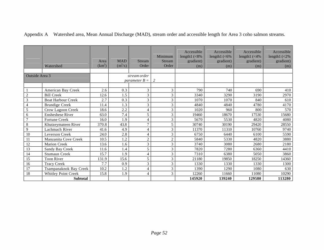
Page 52
Appendix A Watershed area, Mean Annual Discharge (MAD), stream order and accessible length for Area 3 coho salmon streams.
Watershed
Area (km2)
MAD (m3/s)
Stream Order
Minimum Stream
Order
Accessible length1 (<8%
gradient) (m)
Accessible length1 (<6%
gradient) (m)
Accessible length1 (<4%
gradient) (m)
Accessible length1 (<2%
gradient) (m)
Outside Area 3
stream order parameter B = 2
1 American Bay Creek 2.6 0.3 3 3 790 740 690 410 2 Bill Creek 12.6 1.5 3 3 3340 3290 3190 2970 3 Boat Harbour Creek 2.7 0.3 3 3 1070 1070 840 610 4 Brundige Creek 11.4 1.3 3 3 4840 4840 4780 4170 5 Crow Lagoon Creek 18.6 2.2 4 3 1020 960 800 570 6 Ensheshese River 63.0 7.4 5 3 19460 18670 17530 15680 7 Fortune Creek 16.0 1.9 4 3 5670 5530 4820 4080 8 Khutzeymateen River 370.8 43.8 7 5 30740 30190 29420 28550 9 Lachmach River 41.6 4.9 4 3 11370 11310 10760 9740 10 Leverson Creek 24.0 2.8 4 3 6750 6440 6100 5590 11 Manzanita Cove Creek 10.5 1.2 2 2 5840 5330 4820 3880 12 Marion Creek 13.6 1.6 3 3 3740 3080 2680 2180 13 Sandy Bay Creek 11.6 1.4 5 3 7820 7280 6360 4410 14 Stumaun Creek 15.7 1.9 4 3 7310 6380 5050 3860 15 Toon River 131.9 15.6 5 3 21180 19850 18250 14360 16 Tracy Creek 7.7 0.9 3 3 1330 1330 1330 1300 17 Tsampanaknok Bay Creek 10.2 1.2 4 3 1390 1290 1080 630 18 Whitley Point Creek 15.8 1.9 4 3 12260 11660 11080 10290
Subtotal 145920 139240 129580 113280

Page 53
Appendix A (cont).
Watershed Area (km2)
MAD (m3/s)
Stream Order
Minimum Stream
Order
Accessible length1 (<8%
gradient) (m)
Accessible length1 (<6%
gradient) (m)
Accessible length1 (<4%
gradient) (m)
Accessible length1 (<2%
gradient) (m)
Coastal Nass Area
stream order parameter B = 2
19 Bear River 710.5 40.0 7 5 63800 62800 61780 60170 20 Bell Bay Creek 31.6 1.8 5 3 8220 5620 3950 2230 21 Bonanza Creek 31.2 1.8 4 3 5760 5270 4430 3080 22 Cascade Creek 19.6 1.1 4 3 1380 1260 1090 710 23 Chambers Creek 89.9 10.6 4 3 10010 9330 8920 8090 24 Dogfish Bay Creek 21.9 1.2 4 3 7550 6890 6180 5110 25 Donahue Creek 70.8 4.0 5 3 14610 10440 6990 4480 26 Georgie River 160.4 9.0 6 4 29030 25780 20410 12170 27 Illiance River 91.6 5.2 5 3 1560 1550 1480 1480 28 Isaac Creek 14.2 0.8 3 3 2840 2790 2520 2410 29 Kincolith River 225.9 12.7 4 3 30180 29390 28680 27180 30 Kitsault River 258.6 14.6 9 7 25850 25690 25640 25370 31 Kshwan River 175.4 9.9 8 6 18780 18560 18210 16960 32 Kwinamass River 284.0 33.6 6 4 38880 37670 35680 31290 33 Lime Creek 27.9 1.6 4 3 2230 1780 1400 780 34 Lizard Creek 32.2 3.8 4 3 2650 2650 2500 2280 35 Olh Creek 71.6 4.0 5 3 1950 1950 1950 1950 36 Pearce Island No1 17.2 1.0 3 3 2990 2940 2940 2740 37 Roberson Creek 8.0 0.5 3 3 850 690 530 310 38 Rodgers Creek 14.2 0.8 4 3 6060 5740 4890 3600 39 Roundy Creek 16.2 0.9 3 3 1830 1320 940 550 40 Salmon Cove Creek 24.9 1.4 4 3 5340 5160 4860 3730 41 Scowbank Creek 26.3 1.5 3 3 1320 860 550 330 42 Stagoo Creek 78.0 4.4 5 3 27610 26540 24820 21850 43 Tauw Creek 9.4 0.5 3 3 240 180 130 80 44 Wilauks Creek 11.3 0.6 4 3 3520 3410 3350 3090
Subtotal 315040 296260 274820 242020

Page 54
Appendix A (cont).
Watershed Area (km2)
MAD (m3/s)
Stream Order
Minimum Stream
Order
Accessible length1 (<8%
gradient) (m)
Accessible length1 (<6%
gradient) (m)
Accessible length1 (<4%
gradient) (m)
Accessible length1 (<2%
gradient) (m)
Lower Nass River
stream order
parameter B = 2
45 Anliyen Creek (Greenville) 40.7 2.6 4 3 7910 7260 6880 5530
46 Ansedagan Creek 28.5 1.8 4 3 3110 2920 2720 2280 47 Anudol Creek 123.7 7.8 5 3 6410 6380 6380 5950 48 Burton Creek 96.0 11.5 5 3 280 280 220 220 49 Chemainuk Creek 58.1 6.9 4 3 15050 14670 13760 11200 50 Cugiladap Creek 6.2 0.4 3 3 1290 1220 980 500 51 Disangieq Creek 36.4 2.3 4 3 8960 8580 8160 6410 52 Gingietl Creek 14.7 0.9 3 3 1370 920 720 270 53 Ginlulak Creek 43.3 2.7 4 3 6820 6700 5840 5320 54 Gish Creek 14.7 0.9 3 3 7200 6580 5410 3830 55 Giswatz Creek 13.3 0.8 3 3 1670 1440 1190 470 56 Gitwinksihlkw Creek 7.0 0.4 3 3 1070 1000 780 610 57 Iknouk River 112.4 7.1 4 3 25800 24740 23780 21260 58 Inieth Creek 9.5 0.6 3 3 760 710 480 300 59 Ishkeenickh River 579.4 36.6 7 5 70070 68310 64020 53440 60 Keazoah Creek 11.5 0.7 3 3 770 770 650 470 61 Ksemamaith River 68.4 4.3 4 3 2030 2030 1840 1410 62 Kwiniak Creek 248.1 15.7 5 3 11460 10980 10460 9230 63 Kwinyarh Creek 15.6 1.0 3 3 1520 1340 1020 720 64 Monkley Creek 35.7 4.3 4 3 7590 6320 4930 3220 65 Quilgauw Creek 37.0 2.3 4 3 9600 9500 9300 8870 66 Seaskinnish Creek 204.6 12.9 5 3 8710 8530 8390 7580 67 Tseax River 608.3 38.4 6 4 16770 16530 16020 13370 68 Wegiladap Creek 17.0 1.1 4 3 1190 1010 770 590 69 Welda Creek 31.3 3.7 3 3 710 610 560 250 70 Wilyayaanooth Creek 12.7 0.8 3 3 770 690 570 510 71 Zolzap Creek 32.0 2.0 5 3 7810 7630 7280 6880
Subtotal 226700 217650 203110 170690

Page 55
Appendix A (cont).
Watershed Area (km2)
MAD (m3/s)
Stream Order
Minimum Stream
Order
Accessible length1 (<8%
gradient) (m)
Accessible length1 (<6%
gradient) (m)
Accessible length1 (<4%
gradient) (m)
Accessible length1 (<2%
gradient) (m)
Upper Nass River
stream order parameter B = 2
72 Bell-Irving River -Above Teigen 1223.5 83.1 7 5 121590 118880 114320 107860
73 Bell-Irving River -Bowser to Teigen 687.8 46.7 7 5 86790 85160 81910 77900
74 Bell-Irving River -below Bowser 456.1 31.0 7 5 43720 43490 42060 39070
75 Bowser River 1262.0 85.7 7 5 92800 92450 91330 88520 76 Cranberry River 974.8 41.2 7 5 143870 141750 136590 125480 77 Damdochax Creek 737.4 50.1 7 5 62450 62250 61460 57730 78 Hodder Creek 72.3 4.9 5 3 21350 19180 15450 6880 79 Kinskuch River 476.9 32.4 5 3 20 20 20 20 80 Kiteen River 885.5 37.4 7 5 72480 71080 67950 62540 81 Konigus Creek 471.7 32.0 6 4 82 Kotsinta Creek 312.4 21.2 5 3 26210 22290 18220 14900 83 Kshadin Creek 105.1 6.6 5 3 70 70 20 20 84 Kwinageese River 552.3 37.5 6 4 152100 143640 129230 112520 85 Kwinatahl River 306.1 19.3 6 4 8610 8550 8380 7980 86 Meziadin River 735.6 48.9 6 4 110730 104380 93210 78010 87 Muskaboo Creek 614.9 41.8 6 4 88 Panorama Creek 90.6 6.2 5 3 89 Paw Creek 176.7 12.0 6 4 43090 41540 37640 32340

Page 56
Appendix A (cont).
Watershed Area (km2)
MAD (m3/s)
Stream Order
Minimum Stream
Order
Accessible length1 (<8%
gradient) (m)
Accessible length1 (<6%
gradient) (m)
Accessible length1 (<4%
gradient) (m)
Accessible length1 (<2%
gradient) (m)
Upper Nass River (cont)
stream order parameter B = 2
90 Saladamis Creek 75.0 5.1 5 3 17560 15440 11090 6800 91 Sallysout Creek 333.2 22.6 6 4 1670 1670 1370 1120 92 Sanskisoot Creek 103.3 7.0 5 3 30070 23660 16340 11490 93 Sanyam Creek 96.6 6.6 5 3 340 300 260 150 94 Shumal Creek 99.6 6.3 4 3 16360 15610 14560 9680 95 Taft Creek 474.0 32.2 6 4 50000 45030 38040 30370 96 Taylor River 753.2 51.2 7 5 97 Tchitin River 248.2 16.9 6 4 16990 16940 16820 16120 98 Teigen Creek 351.7 23.9 6 4 64090 60480 53750 43810 99 Treaty Creek 427.1 29.0 6 4 51920 49380 46390 43860 100 Upper Nass River 735.6 50.0 6 4 101 Vile Creek 188.0 12.8 5 3 49490 40590 31760 23140 102 White River 954.0 64.8 6 4 144600 141970 135020 123070
Subtotal 1802920 1705560 1556900 1360220
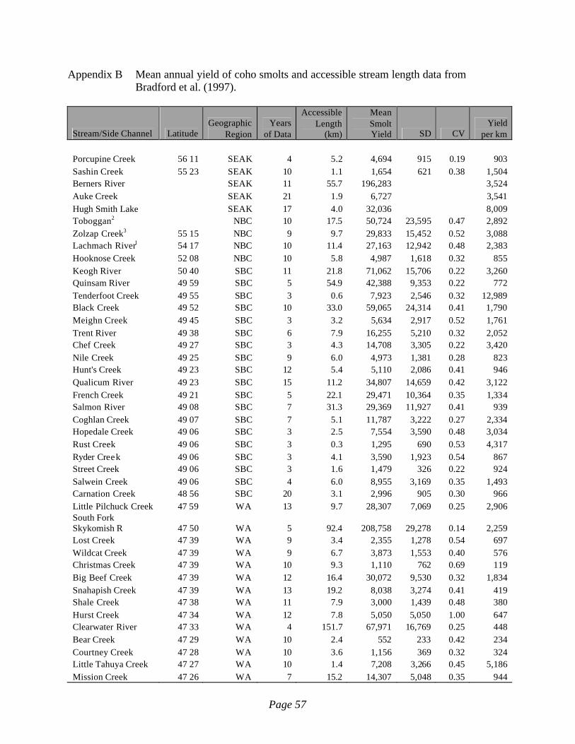
Page 57
Appendix B Mean annual yield of coho smolts and accessible stream length data from Bradford et al. (1997).
Stream/Side Channel Latitude Geographic
Region Years
of Data
Accessible Length
(km)
Mean Smolt Yield SD CV
Yield per km
Porcupine Creek 56 11 SEAK 4 5.2 4,694 915 0.19 903 Sashin Creek 55 23 SEAK 10 1.1 1,654 621 0.38 1,504 Berners River SEAK 11 55.7 196,283 3,524 Auke Creek SEAK 21 1.9 6,727 3,541 Hugh Smith Lake SEAK 17 4.0 32,036 8,009 Toboggan2 NBC 10 17.5 50,724 23,595 0.47 2,892 Zolzap Creek3 55 15 NBC 9 9.7 29,833 15,452 0.52 3,088 Lachmach River1 54 17 NBC 10 11.4 27,163 12,942 0.48 2,383 Hooknose Creek 52 08 NBC 10 5.8 4,987 1,618 0.32 855 Keogh River 50 40 SBC 11 21.8 71,062 15,706 0.22 3,260 Quinsam River 49 59 SBC 5 54.9 42,388 9,353 0.22 772 Tenderfoot Creek 49 55 SBC 3 0.6 7,923 2,546 0.32 12,989 Black Creek 49 52 SBC 10 33.0 59,065 24,314 0.41 1,790 Meighn Creek 49 45 SBC 3 3.2 5,634 2,917 0.52 1,761 Trent River 49 38 SBC 6 7.9 16,255 5,210 0.32 2,052 Chef Creek 49 27 SBC 3 4.3 14,708 3,305 0.22 3,420 Nile Creek 49 25 SBC 9 6.0 4,973 1,381 0.28 823 Hunt's Creek 49 23 SBC 12 5.4 5,110 2,086 0.41 946 Qualicum River 49 23 SBC 15 11.2 34,807 14,659 0.42 3,122 French Creek 49 21 SBC 5 22.1 29,471 10,364 0.35 1,334 Salmon River 49 08 SBC 7 31.3 29,369 11,927 0.41 939 Coghlan Creek 49 07 SBC 7 5.1 11,787 3,222 0.27 2,334 Hopedale Creek 49 06 SBC 3 2.5 7,554 3,590 0.48 3,034 Rust Creek 49 06 SBC 3 0.3 1,295 690 0.53 4,317 Ryder Creek 49 06 SBC 3 4.1 3,590 1,923 0.54 867 Street Creek 49 06 SBC 3 1.6 1,479 326 0.22 924 Salwein Creek 49 06 SBC 4 6.0 8,955 3,169 0.35 1,493 Carnation Creek 48 56 SBC 20 3.1 2,996 905 0.30 966 Little Pilchuck Creek 47 59 WA 13 9.7 28,307 7,069 0.25 2,906 South Fork Skykomish R 47 50 WA 5 92.4 208,758 29,278 0.14 2,259 Lost Creek 47 39 WA 9 3.4 2,355 1,278 0.54 697 Wildcat Creek 47 39 WA 9 6.7 3,873 1,553 0.40 576 Christmas Creek 47 39 WA 10 9.3 1,110 762 0.69 119 Big Beef Creek 47 39 WA 12 16.4 30,072 9,530 0.32 1,834 Snahapish Creek 47 39 WA 13 19.2 8,038 3,274 0.41 419 Shale Creek 47 38 WA 11 7.9 3,000 1,439 0.48 380 Hurst Creek 47 34 WA 12 7.8 5,050 5,050 1.00 647 Clearwater River 47 33 WA 4 151.7 67,971 16,769 0.25 448 Bear Creek 47 29 WA 10 2.4 552 233 0.42 234 Courtney Creek 47 28 WA 10 3.6 1,156 369 0.32 324 Little Tahuya Creek 47 27 WA 10 1.4 7,208 3,266 0.45 5,186 Mission Creek 47 26 WA 7 15.2 14,307 5,048 0.35 944

Page 58
Appendix B (cont).
Stream/Side Channel Latitude Geographic
Region Years
of Data
Accessible Length
(km)
Mean Smolt Yield SD CV
Yield per km
Minter Creek 47 22 WA 11 16.7 28,456 7,337 0.26 1,704 Harris Creek 47 21 WA 9 11.6 25,772 7,718 0.30 2,220 Mill Creek 47 12 WA 12 16.5 24,809 7,997 0.32 1,503 Deschutes River 46 57 WA 6 54.0 64,675 25,825 0.40 1,198 Gnat Creek 46 12 OR 5 4.8 2,048 1,041 0.51 427 Spring Creek 45 37 OR 10 0.5 1,360 583 0.43 2,894 Sand Creek 45 17 OR 3 9.7 1,207 133 0.11 124 Fish Creek 45 09 OR 3 16.7 2,689 373 0.14 161 Deer Creek 44 32 OR 15 2.3 2,014 617 0.31 868 Flynn Creek 44 31 OR 14 1.4 667 366 0.55 466 Needle Branch Creek 44 31 OR 14 1.0 283 138 0.49 292 Waddell Creek 37 06 CA 4 10.3 6,445 4,266 0.66 626 SEAK Mean 12.6 13.6 0.29 3,496 NBC Mean 9.8 11.1 0.45 2,305 SBC Mean 6.9 11.8 0.36 2,481 BC Mean 7.4 11.7 0.37 2,451 WA Mean 9.6 24.8 0.41 1,311 OR Mean 9.1 5.2 0.36 747 Overall Mean 8.8 15.4 0.39 1,913 1 Lachmach mean for smolt years 1991-2000 (Joel Sawada, pers. comm.). 2 Toboggan Creek mean for smolt years 1991-2000 (Joel Sawada, pers. comm.). 3 Zolzap Creek mean for smolt years 1992-2000 (Baxter et al. 2001) 4 Hunts Creek Length modified according to Myers

Page 59
Appendix C Smolt yield estimates for Area 3 coho streams using 2 different models.
Total Smolts
Watershed Area (km2)
Stream Order
Stream Length
(m) Model 1 Model 2 Outside Area 3 Beta= 2 G8 Estimate St. Dev. Estimate St. Dev.
1 American Bay Creek 2.6 3
790
2,886
2,540
1,882
897
2 Bill Creek 12.6 3 3,340 9,464 7,903 7,958 3,792
3 Boat Harbour Creek 2.7 3
1,070
3,698
3,204
2,550
1,215
4 Brundige Creek 11.4 3 4,840 12,898 10,723 11,532 5,495
5 Crow Lagoon Creek 18.6 4
1,020
3,556
3,088
2,430
1,158
6 Ensheshese River 63.0 5 19,460 41,781 35,385 46,368 22,092 7 Fortune Creek 16.0 4 5,670 14,726 12,235 13,510 6,437
8 Khutzeymateen River 370.8 7
30,740
61,781
53,257
73,245
34,898
9 Lachmach River 41.6 4 11,370 26,465 22,111 27,091 12,908 10 Leverson Creek 24.0 4 6,750 17,047 14,165 16,083 7,663
11 Manzanita Cove Creek 10.5 2
5,840
15,095
12,541
13,915
6,630
12 Marion Creek 13.6 3 3,740 10,399 8,669 8,911 4,246 13 Sandy Bay Creek 11.6 5 7,820 19,293 16,044 18,633 8,878 14 Stumaun Creek 15.7 4 7,310 18,229 15,152 17,418 8,299 15 Toon River 131.9 5 21,180 44,912 38,147 50,466 24,045 16 Tracy Creek 7.7 3 1,330 4,420 3,793 3,169 1,510
17 Tsampanaknok Bay Creek 10.2 4
1,390
4,583
3,926
3,312
1,578
18 Whitley Point Creek 15.8 4
12,260
28,209
23,602
29,212
13,918
Subtotal 145,920 339,441 88,841 347,686 54,838

Page 60
Appendix C (cont).
Total Smolts
Watershed Area (km2)
Stream Order
Stream Length
(m) Model 1 Model 2 Coastal Nass Area Beta= 2
19 Bear River 710.5 7 63,800 115,974 103,943 152,017 72,429 20 Bell Bay Creek 31.6 5 8,220 20,122 16,739 19,586 9,332 21 Bonanza Creek 31.2 4 5,760 14,922 12,397 13,724 6,539 22 Cascade Creek 19.6 4 1,380 4,556 3,904 3,288 1,567 23 Chambers Creek 89.9 4 10,010 23,761 19,812 23,851 11,364 24 Dogfish Bay Creek 21.9 4 7,550 18,731 15,572 17,989 8,571 25 Donahue Creek 70.8 5 14,610 32,735 27,497 34,811 16,586 26 Georgie River 160.4 6 29,030 58,821 50,578 69,170 32,956 27 Illiance River 91.6 5 1,560 5,040 4,297 3,717 1,771 28 Isaac Creek 14.2 3 2,840 8,271 6,928 6,767 3,224 29 Kincolith River 225.9 4 30,180 60,814 52,380 71,910 34,262 30 Kitsault River 258.6 9 25,850 53,254 45,571 61,593 29,346 31 Kshwan River 175.4 8 18,780 40,533 34,289 44,747 21,320 32 Kwinamass River 284.0 6 38,880 75,605 65,904 92,640 44,139 33 Lime Creek 27.9 4 2,230 6,768 5,704 5,313 2,532 34 Lizard Creek 32.2 4 2,650 7,809 6,551 6,314 3,008 35 Olh Creek 71.6 5 1,950 6,058 5,125 4,646 2,214 36 Pearce Island No1 17.2 3 2,990 8,632 7,223 7,124 3,394 37 Roberson Creek 8.0 3 850 3,063 2,685 2,025 965 38 Rodgers Creek 14.2 4 6,060 15,571 12,936 14,439 6,880 39 Roundy Creek 16.2 3 1,830 5,748 4,874 4,360 2,078
40 Salmon Cove Creek 24.9 4 5,340
14,004
11,637 12,724
6,062
41 Scowbank Creek 26.3 3 1,320 4,393 3,771 3,145 1,499 42 Stagoo Creek 78.0 5 27,610 56,345 48,346 65,787 31,344 43 Tauw Creek 9.4 3 240 1,102 1,050 572 272 44 Wilauks Creek 11.3 4 3,520 9,887 8,249 8,387 3,996
Subtotal 315,040 672,516 168,869 750,650 111,873

Page 61
Appendix C (cont).
Total Smolts
Watershed Area (km2)
Stream Order
Stream Length
(m) Model 1 Model 2 Lower Nass Area Beta= 2
45 Anliyen Creek (Greenville) 40.7 4
7,910
19,480
16,200
24,429
12,652
46 Ansedagan Creek 28.5 4 3,110 8,919 7,457 9,605 4,975 47 Anudol Creek 123.7 5 6,410 16,322 13,561 19,796 10,253 48 Burton Creek 96.0 5 280 1,247 1,175 865 448 49 Chemainuk Creek 58.1 4 15,050 33,571 28,220 46,479 24,073 50 Cugiladap Creek 6.2 3 1,290 4,311 3,704 3,984 2,063 51 Disangieq Creek 36.4 4 8,960 21,639 18,016 27,671 14,332 52 Gingietl Creek 14.7 3 1,370 4,529 3,882 4,231 2,191 53 Ginlulak Creek 43.3 4 6,820 17,195 14,289 21,062 10,909 54 Gish Creek 14.7 3 7,200 17,998 14,959 22,236 11,517 55 Giswatz Creek 13.3 3 1,670 5,331 4,534 5,158 2,671
56 Gitwinksihlkw Creek 7.0 3
1,070 3,698 3,204 3,305
1,712
57 Iknouk River 112.4 4 25,800 53,166 45,492 79,679 41,268 58 Inieth Creek 9.5 3 760 2,796 2,466 2,347 1,216 59 Ishkeenickh River 579.4 7 70,070 125,796 113,412 216,400 112,080 60 Keazoah Creek 11.5 3 770 2,826 2,490 2,378 1,232 61 Ksemamaith River 68.4 4 2,030 6,262 5,292 6,269 3,247 62 Kwiniak Creek 248.1 5 11,460 26,642 22,262 35,392 18,331 63 Kwinyarh Creek 15.6 3 1,520 4,933 4,210 4,694 2,431 64 Monkley Creek 35.7 4 7,590 18,814 15,642 23,440 12,140 65 Quilgauw Creek 37.0 4 9,600 22,936 19,113 29,648 15,356 66 Seaskinnish Creek 204.6 5 8,710 21,128 17,586 26,899 13,932 67 Tseax River 608.3 6 16,770 36,807 31,031 51,791 26,824 68 Wegiladap Creek 17.0 4 1,190 4,034 3,479 3,675 1,903 69 Welda Creek 31.3 3 710 2,645 2,342 2,193 1,136
70 Wilyayaanooth Creek 12.7 3
770
2,826
2,490
2,378
1,232
71 Zolzap Creek 32.0 5 7,810 19,273 16,026 24,120 12,492 Subtotal 226,700 505,125 140,571 700,126 132,006

Page 62
Appendix C (cont).
Total Smolts
Watershed Area (km2)
Stream Order
Stream Length
(m) Model 1 Model 2 Upper Nass River Beta= 2
72 Bell-Irving River -Above Teigen 1223.5 7
121,590
203,316
190,462
351,625 163,562
73 Bell-Irving River -Bowser to Teigen 687.8 7
86,790
151,510
138,540
250,987 116,749
74 Bell-Irving River -below Bowser 456.1 7
43,720
83,648
73,358
126,434
58,812
75 Bowser River 1262.0 7 92,800 160,605 147,537 268,368 124,834 76 Cranberry River 974.8 7 143,870 235,576 223,545 416,057 193,533 77 Damdochax Creek 737.4 7 62,450 113,844 101,900 180,599 84,007 78 Hodder Creek 72.3 5 21,350 45,220 38,419 61,742 28,720 79 Kinskuch River 476.9 5 20 156 189 58 27 80 Kiteen River 885.5 7 72,480 129,544 117,045 209,604 97,500 81 Konigus Creek 471.7 6 82 Kotsinta Creek 312.4 5 26,210 53,889 46,140 75,797 35,258 83 Kshadin Creek 105.1 5 70 414 441 202 94 84 Kwinageese River 552.3 6 152,100 247,348 235,745 439,857 204,604 85 Kwinatahl River 306.1 6 8,610 20,923 17,414 24,899 11,582 86 Meziadin River 735.6 6 110,730 187,357 174,299 320,219 148,953 87 Muskaboo Creek 614.9 6 88 Panorama Creek 90.6 5 89 Paw Creek 176.7 6 43,090 82,607 72,390 124,612 57,964 90 Saladamis Creek 75.0 5 17,560 38,278 32,315 50,782 23,622 91 Sallysout Creek 333.2 6 1,670 5,331 4,534 4,829 2,246 92 Sanskisoot Creek 103.3 5 30,070 60,623 52,208 86,959 40,450 93 Sanyam Creek 96.6 5 340 1,457 1,353 983 457 94 Shumal Creek 99.6 4 16,360 36,040 30,363 47,311 22,007 95 Taft Creek 474.0 6 50,000 93,921 82,975 144,595 67,260 96 Taylor River 753.2 7 97 Tchitin River 248.2 6 16,990 37,218 31,389 49,133 22,855 98 Teigen Creek 351.7 6 64,090 116,430 104,382 185,341 86,213 99 Treaty Creek 427.1 6 51,920 97,030 85,905 150,147 69,842
100 Upper Nass River 735.6 6 101 Vile Creek 188.0 5 49,490 93,093 82,197 143,120 66,574 102 White River 954.0 6 144,600 236,623 224,627 418,168 194,515
Subtotal 1,802,920 3,172,683 665,501 5,213,851 566,449
Model 1 = Nonlinear relation between stream length and smolt density for streams from British Co lumbia and Southeast Alaska, Bradford et al. (1997).
Model 2 = Lachmach mean smolt density applied to Outside Area 3 and Coastal Nass; Zolzap mean smolts density applied to Lower Nass; and Toboggan Creek mean smolt densities applied to Upper Nass.

Page 63
Appendix D Estimate of the required number of coho spawners assuming Model 1 smolt production (regional database).
Watershed
Stream Length
(m) Stream
Order Smolts1
Produced Fry2
Produced Required3
Eggs Female 5
fecundity Spawners Spawner/
km
Percent of Total Nass
escapement egg-fry = 19.8% fry-smolt = 7.6% Outside Area 3
1 American Bay Creek 790 3 2,886 37,972 191,777 3000 128 162 0.06% 2 Bill Creek 3340 3 9,464 124,530 628,938 3000 419 126 0.20% 3 Boat Harbour Creek 1070 3 3,698 48,655 245,733 3000 164 153 0.08% 4 Brundige Creek 4840 3 12,898 169,706 857,101 3000 571 118 0.28% 5 Crow Lagoon Creek 1020 4 3,556 46,786 236,292 3000 158 154 0.08% 6 Ensheshese River 19460 5 41,781 549,747 2,776,501 3000 1,851 95 0.90% 7 Fortune Creek 5670 4 14,726 193,761 978,590 3000 652 115 0.32% 8 Khutzeymateen River 30740 7 61,781 812,904 4,105,575 3000 2,737 89 1.33% 9 Lachmach River 11370 4 26,465 348,220 1,758,685 3000 1,172 103 0.57%
10 Leverson Creek 6750 4 17,047 224,301 1,132,832 3000 755 112 0.37% 11 Manzanita Cove Creek 5840 2 15,095 198,621 1,003,137 3000 669 115 0.32% 12 Marion Creek 3740 3 10,399 136,833 691,074 3000 461 123 0.22% 13 Sandy Bay Creek 7820 5 19,293 253,860 1,282,123 3000 855 109 0.41% 14 Stumaun Creek 7310 4 18,229 239,849 1,211,361 3000 808 110 0.39% 15 Toon River 21180 5 44,912 590,952 2,984,606 3000 1,990 94 0.96% 16 Tracy Creek 1330 3 4,420 58,158 293,730 3000 196 147 0.09%
17 Tsampanaknok Bay Creek 1390 4 4,583 60,306 304,576 3000 203 146 0.10%
18 Whitley Point Creek 12260 4 28,209 371,173 1,874,611 3000 1,250 102 0.61% Subtotal 145,920 339,441 4,466,334 22,557,243 15,038 121 7.29%

Page 64
Appendix D (cont).
Watershed
Stream Length
(m) Stream
Order Smolts1
Produced Fry2
Produced Required3
Eggs Female 5
fecundity Spawners Spawner/
km
Percent of Total Nass
escapement egg-fry = 19.8% fry-smolt = 7.6% Coastal Nass Area
19 Bear River 63800 7 115,974 1,525,970 7,706,917 3000 5,138 81 2.49% 20 Bell Bay Creek 8220 5 20,122 264,757 1,337,156 3000 891 108 0.43% 21 Bonanza Creek 5760 4 14,922 196,337 991,599 3000 661 115 0.32% 22 Cascade Creek 1380 4 4,556 59,949 302,773 3000 202 146 0.10% 23 Chambers Creek 10010 4 23,761 312,649 1,579,033 3000 1,053 105 0.51% 24 Dogfish Bay Creek 7550 4 18,731 246,460 1,244,746 3000 830 110 0.40% 25 Donahue Creek 14610 5 32,735 430,722 2,175,362 3000 1,450 99 0.70% 26 Georgie River 29030 6 58,821 773,954 3,908,859 3000 2,606 90 1.26% 27 Illiance River 1560 5 5,040 66,311 334,903 3000 223 143 0.11% 28 Isaac Creek 2840 3 8,271 108,824 549,618 3000 366 129 0.18% 29 Kincolith River 30180 4 60,814 800,180 4,041,312 3000 2,694 89 1.31% 30 Kitsault River 25850 9 53,254 700,714 3,538,960 3000 2,359 91 1.14% 31 Kshwan River 18780 8 40,533 533,325 2,693,560 3000 1,796 96 0.87% 32 Kwinamass River 38880 6 75,605 994,800 5,024,244 3000 3,349 86 1.62% 33 Lime Creek 2230 4 6,768 89,059 449,791 3000 300 134 0.15% 34 Lizard Creek 2650 4 7,809 102,747 518,922 3000 346 131 0.17% 35 Olh Creek 1950 5 6,058 79,708 402,565 3000 268 138 0.13% 36 Pearce Island No1 2990 3 8,632 113,578 573,625 3000 382 128 0.19% 37 Roberson Creek 850 3 3,063 40,309 203,579 3000 136 160 0.07% 38 Rodgers Creek 6060 4 15,571 204,880 1,034,747 3000 690 114 0.33% 39 Roundy Creek 1830 3 5,748 75,636 382,000 3000 255 139 0.12% 40 Salmon Cove Creek 5340 4 14,004 184,264 930,627 3000 620 116 0.30% 41 Scowbank Creek 1320 3 4,393 57,799 291,914 3000 195 147 0.09% 42 Stagoo Creek 27610 5 56,345 741,385 3,744,368 3000 2,496 90 1.21% 43 Tauw Creek 240 3 1,102 14,493 73,199 3000 49 203 0.02% 44 Wilauks Creek 3520 4 9,887 130,092 657,033 3000 438 124 0.21%
Sub total 315,040 672,516 8,848,900 44,691,414 29,794 120 14.44%

Page 65
Appendix D (cont).
Watershed
Stream Length
(m) Stream
Order Smolts1
Produced Fry2
Produced Required3
Eggs Female 5
fecundity Spawners Spawner/
km
Percent of Total Nass
escapement egg-fry = 19.8% fry-smolt = 7.6% Lower Nass Area
45 Anliyen Creek (Greenville) 7910 4 19,480 256,319 1,294,540 2500 1,036 131 0.50%
46 Ansedagan Creek 3110 4 8,919 117,354 592,697 2500 474 152 0.23% 47 Anudol Creek 6410 5 16,322 214,769 1,084,693 2500 868 135 0.42% 48 Burton Creek 280 5 1,247 16,402 82,836 2500 66 237 0.03% 49 Chemainuk Creek 15050 4 33,571 441,719 2,230,903 2500 1,785 119 0.87% 50 Cugiladap Creek 1290 3 4,311 56,718 286,455 2500 229 178 0.11% 51 Disangieq Creek 8960 4 21,639 284,719 1,437,976 2500 1,150 128 0.56% 52 Gingietl Creek 1370 3 4,529 59,592 300,969 2500 241 176 0.12% 53 Ginlulak Creek 6820 4 17,195 226,254 1,142,698 2500 914 134 0.44% 54 Gish Creek 7200 3 17,998 236,809 1,196,007 2500 957 133 0.46% 55 Giswatz Creek 1670 3 5,331 70,139 354,238 2500 283 170 0.14% 56 Gitwinksihlkw Creek 1070 3 3,698 48,655 245,733 2500 197 184 0.10% 57 Iknouk River 25800 4 53,166 699,554 3,533,099 2500 2,826 110 1.37% 58 Inieth Creek 760 3 2,796 36,792 185,820 2500 149 196 0.07% 59 Ishkeenickh River 70070 7 125,796 1,655,216 8,359,679 2500 6,688 95 3.24% 60 Keazoah Creek 770 3 2,826 37,186 187,810 2500 150 195 0.07% 61 Ksemamaith River 2030 4 6,262 82,400 416,162 2500 333 164 0.16% 62 Kwiniak Creek 11460 5 26,642 350,552 1,770,464 2500 1,416 124 0.69% 63 Kwinyarh Creek 1520 3 4,933 64,908 327,818 2500 262 173 0.13% 64 Monkley Creek 7590 4 18,814 247,559 1,250,296 2500 1,000 132 0.48% 65 Quilgauw Creek 9600 4 22,936 301,795 1,524,216 2500 1,219 127 0.59% 66 Seaskinnish Creek 8710 5 21,128 278,003 1,404,053 2500 1,123 129 0.54% 67 Tseax River 16770 6 36,807 484,302 2,445,968 2500 1,957 117 0.95% 68 Wegiladap Creek 1190 4 4,034 53,084 268,101 2500 214 180 0.10% 69 Welda Creek 710 3 2,645 34,808 175,799 2500 141 198 0.07% 70 Wilyayaanooth Creek 770 3 2,826 37,186 187,810 2500 150 195 0.07% 71 Zolzap Creek 7810 5 19,273 253,587 1,280,742 2500 1,025 131 0.50%
Sub total 226,700 505,125 6,646,381 33,567,582 26,854 153 13.02%

Page 66
Appendix D (cont).
Watershed
Stream Length
(m) Stream
Order Smolts1
Produced Fry2
Produced Required3
Eggs Female 5
fecundity Spawners Spawner/
km
Percent of Total Nass
escapement egg-fry = 19.8% fry-smolt = 7.6% Upper Nass Area
72 Bell-Irving River -Above Teigen 121590 7
203,316 2,675,215 13,511,187 2500 10,809 89 5.24%
73 Bell-Irving River -Bowser to Teigen 86790 7
151,510 1,993,547 10,068,420 2500 8,055 93 3.90%
74 Bell-Irving River -below Bowser 43720 7
83,648 1,100,627 5,558,720 2500 4,447 102 2.16%
75 Bowser River 92800 7 160,605 2,113,227 10,672,863 2500 8,538 92 4.14% 76 Cranberry River 143870 7 235,576 3,099,682 15,654,959 2500 12,524 87 6.07% 77 Damdochax Creek 62450 7 113,844 1,497,947 7,565,389 2500 6,052 97 2.93% 78 Hodder Creek 21350 5 45,220 595,000 3,005,050 2500 2,404 113 1.17% 79 Kinskuch River 20 5 156 2,051 10,358 2500 8 414 0.00% 80 Kiteen River 72480 7 129,544 1,704,523 8,608,703 2500 6,887 95 3.34% 81 Konigus Creek 6 82 Kotsinta Creek 26210 5 53,889 709,062 3,581,120 2500 2,865 109 1.39% 83 Kshadin Creek 70 5 414 5,447 27,510 2500 22 314 0.01% 84 Kwinageese River 152100 6 247,348 3,254,576 16,437,255 2500 13,150 86 6.37% 85 Kwinatahl River 8610 6 20,923 275,308 1,390,446 2500 1,112 129 0.54% 86 Meziadin River 110730 6 187,357 2,465,223 12,450,622 2500 9,960 90 4.83% 87 Muskaboo Creek 6 88 Panorama Creek 5 89 Paw Creek 43090 6 82,607 1,086,938 5,489,585 2500 4,392 102 2.13%

Page 67
Appendix D (cont).
Watershed
Stream Length
(m) Stream
Order Smolts1
Produced Fry2
Produced Required3
Eggs Female 5
fecundity Spawners Spawner/
km
Percent of Total Nass
escapement egg-fry = 19.8% fry-smolt = 7.6% Upper Nass Area (cont) 90 Saladamis Creek 17560 5 38,278 503,659 2,543,732 2500 2,035 116 0.99% 91 Sallysout Creek 1670 6 5,331 70,139 354,238 2500 283 170 0.14% 92 Sanskisoot Creek 30070 5 60,623 797,677 4,028,671 2500 3,223 107 1.56% 93 Sanyam Creek 340 5 1,457 19,174 96,839 2500 77 228 0.04% 94 Shumal Creek 16360 4 36,040 474,207 2,394,986 2500 1,916 117 0.93% 95 Taft Creek 50000 6 93,921 1,235,807 6,241,451 2500 4,993 100 2.42% 96 Taylor River 7 97 Tchitin River 16990 6 37,218 489,704 2,473,255 2500 1,979 116 0.96% 98 Teigen Creek 64090 6 116,430 1,531,980 7,737,272 2500 6,190 97 3.00% 99 Treaty Creek 51920 6 97,030 1,276,709 6,448,023 2500 5,158 99 2.50% 100 Upper Nass River 6 101 Vile Creek 49490 5 93,093 1,224,911 6,186,418 2500 4,949 100 2.40% 102 White River 144600 6 236,623 3,113,460 15,724,544 2500 12,580 87 6.10% Sub total 1,802,920 3,172,683 41,745,832 210,837,537 168,670 129 65.25%

Page 68
Appendix E Estimate of the required number of coho spawners assuming Model 2 smolt production (local indicators).
Watershed
Stream Length
(m) Stream
Order Smolts1
Produced Fry2
Produced Required3
Eggs Female 5
fecundity Spawners Spawner/
km
Percent of Total Nass
escapement egg-fry = 19.8% fry-smolt = 7.6% Outside Area 3
1 American Bay Creek 790 3 1,882 24,833 125,419 3000 84 106 0.03% 2 Bill Creek 3340 3 7,958 104,990 530,254 3000 354 106 0.12% 3 Boat Harbour Creek 1070 3 2,550 33,635 169,872 3000 113 106 0.04% 4 Brundige Creek 4840 3 11,532 152,142 768,392 3000 512 106 0.17% 5 Crow Lagoon Creek 1020 4 2,430 32,063 161,934 3000 108 106 0.04% 6 Ensheshese River 19460 5 46,368 611,710 3,089,445 3000 2,060 106 0.67% 7 Fortune Creek 5670 4 13,510 178,232 900,162 3000 600 106 0.20% 8 Khutzeymateen River 30740 7 73,245 966,288 4,880,244 3000 3,253 106 1.06% 9 Lachmach River 11370 4 27,091 357,407 1,805,087 3000 1,203 106 0.39%
10 Leverson Creek 6750 4 16,083 212,181 1,071,622 3000 714 106 0.23% 11 Manzanita Cove Creek 5840 2 13,915 183,576 927,151 3000 618 106 0.20% 12 Marion Creek 3740 3 8,911 117,564 593,758 3000 396 106 0.13% 13 Sandy Bay Creek 7820 5 18,633 245,816 1,241,493 3000 828 106 0.27% 14 Stumaun Creek 7310 4 17,418 229,784 1,160,526 3000 774 106 0.25% 15 Toon River 21180 5 50,466 665,777 3,362,510 3000 2,242 106 0.73% 16 Tracy Creek 1330 3 3,169 41,808 211,149 3000 141 106 0.05%
17 Tsampanaknok Bay Creek 1390 4 3,312 43,694 220,675 3000 147 106 0.05%
18 Whitley Point Creek 12260 4 29,212 385,384 1,946,382 3000 1,298 106 0.42% Subtotal 145,920 347,686 4,586,883 23,166,077 15,444 106 5.04%

Page 69
Appendix E (cont).
Watershed
Stream Length
(m) Stream
Order Smolts1
Produced Fry2
Produced Required3
Eggs Female 5
fecundity Spawners Spawner/
km
Percent of Total Nass
escapement egg-fry = 19.8% fry-smolt = 7.6% Coastal Nass Area
19 Bear River 63800 7 152,017 2,005,504 10,128,808 3000 6,753 106 2.20% 20 Bell Bay Creek 8220 5 19,586 258,389 1,304,997 3000 870 106 0.28% 21 Bonanza Creek 5760 4 13,724 181,061 914,450 3000 610 106 0.20% 22 Cascade Creek 1380 4 3,288 43,379 219,087 3000 146 106 0.05% 23 Chambers Creek 10010 4 23,851 314,657 1,589,175 3000 1,059 106 0.35% 24 Dogfish Bay Creek 7550 4 17,989 237,328 1,198,629 3000 799 106 0.26% 25 Donahue Creek 14610 5 34,811 459,254 2,319,465 3000 1,546 106 0.50% 26 Georgie River 29030 6 69,170 912,536 4,608,767 3000 3,073 106 1.00% 27 Illiance River 1560 5 3,717 49,037 247,664 3000 165 106 0.05% 28 Isaac Creek 2840 3 6,767 89,273 450,875 3000 301 106 0.10% 29 Kincolith River 30180 4 71,910 948,685 4,791,339 3000 3,194 106 1.04% 30 Kitsault River 25850 9 61,593 812,575 4,103,914 3000 2,736 106 0.89% 31 Kshwan River 18780 8 44,747 590,335 2,981,489 3000 1,988 106 0.65% 32 Kwinamass River 38880 6 92,640 1,222,163 6,172,540 3000 4,115 106 1.34% 33 Lime Creek 2230 4 5,313 70,098 354,032 3000 236 106 0.08% 34 Lizard Creek 2650 4 6,314 83,301 420,711 3000 280 106 0.09% 35 Olh Creek 1950 5 4,646 61,297 309,580 3000 206 106 0.07% 36 Pearce Island No1 2990 3 7,124 93,988 474,689 3000 316 106 0.10% 37 Roberson Creek 850 3 2,025 26,719 134,945 3000 90 106 0.03% 38 Rodgers Creek 6060 4 14,439 190,491 962,078 3000 641 106 0.21% 39 Roundy Creek 1830 3 4,360 57,525 290,529 3000 194 106 0.06% 40 Salmon Cove Creek 5340 4 12,724 167,859 847,772 3000 565 106 0.18% 41 Scowbank Creek 1320 3 3,145 41,493 209,562 3000 140 106 0.05% 42 Stagoo Creek 27610 5 65,787 867,899 4,383,329 3000 2,922 106 0.95% 43 Tauw Creek 240 3 572 7,544 38,102 3000 25 106 0.01% 44 Wilauks Creek 3520 4 8,387 110,648 558,831 3000 373 106 0.12%
Sub total 315,040 750,650 9,903,041 50,015,357 33,344 106 10.88%

Page 70
Appendix E (cont).
Watershed
Stream Length
(m) Stream
Order Smolts1
Produced Fry2
Produced Required3
Eggs Female 5
fecundity Spawners Spawner/
km
Percent of Total Nass
escapement egg-fry = 19.8% fry-smolt = 7.6% Lower Nass Area
45 Anliyen Creek (Greenville) 7910 4 24,429 322,279 1,627,671 2500 1,302 165 0.43%
46 Ansedagan Creek 3110 4 9,605 126,711 639,957 2500 512 165 0.17% 47 Anudol Creek 6410 5 19,796 261,164 1,319,011 2500 1,055 165 0.34% 48 Burton Creek 280 5 865 11,408 57,617 2500 46 165 0.02% 49 Chemainuk Creek 15050 4 46,479 613,186 3,096,897 2500 2,478 165 0.81% 50 Cugiladap Creek 1290 3 3,984 52,559 265,448 2500 212 165 0.07% 51 Disangieq Creek 8960 4 27,671 365,059 1,843,734 2500 1,475 165 0.48% 52 Gingietl Creek 1370 3 4,231 55,818 281,910 2500 226 165 0.07% 53 Ginlulak Creek 6820 4 21,062 277,869 1,403,378 2500 1,123 165 0.37% 54 Gish Creek 7200 3 22,236 293,351 1,481,572 2500 1,185 165 0.39% 55 Giswatz Creek 1670 3 5,158 68,041 343,642 2500 275 165 0.09% 56 Gitwinksihlkw Creek 1070 3 3,305 43,595 220,178 2500 176 165 0.06% 57 Iknouk River 25800 4 79,679 1,051,175 5,308,966 2500 4,247 165 1.39% 58 Inieth Creek 760 3 2,347 30,965 156,388 2500 125 165 0.04% 59 Ishkeenickh River 70070 7 216,400 2,854,878 14,418,576 2500 11,535 165 3.76% 60 Keazoah Creek 770 3 2,378 31,372 158,446 2500 127 165 0.04% 61 Ksemamaith River 2030 4 6,269 82,709 417,721 2500 334 165 0.11% 62 Kwiniak Creek 11460 5 35,392 466,917 2,358,169 2500 1,887 165 0.62% 63 Kwinyarh Creek 1520 3 4,694 61,930 312,776 2500 250 165 0.08% 64 Monkley Creek 7590 4 23,440 309,241 1,561,824 2500 1,249 165 0.41% 65 Quilgauw Creek 9600 4 29,648 391,135 1,975,429 2500 1,580 165 0.52% 66 Seaskinnish Creek 8710 5 26,899 354,874 1,792,291 2500 1,434 165 0.47% 67 Tseax River 16770 6 51,791 683,264 3,450,828 2500 2,761 165 0.90% 68 Wegiladap Creek 1190 4 3,675 48,484 244,871 2500 196 165 0.06% 69 Welda Creek 710 3 2,193 28,928 146,099 2500 117 165 0.04% 70 Wilyayaanooth Creek 770 3 2,378 31,372 158,446 2500 127 165 0.04% 71 Zolzap Creek 7810 5 24,120 318,205 1,607,094 2500 1,286 165 0.42%
Sub total 226,700 700,126 9,236,490 46,648,940 37,319 165 12.18%

Page 71
Appendix E (cont).
Watershed
Stream Length
(m) Stream
Order Smolts1
Produced Fry2
Produced Required3
Eggs Female 5
fecundity Spawners Spawner/
km
Percent of Total Nass
escapement egg-fry = 19.8% fry-smolt = 7.6% Upper Nass Area
72 Bell-Irving River -Above Teigen 121590 7 351,625 4,638,856 23,428,563 2500 18,743 154 6.12%
73 Bell-Irving River -Bowser to Teigen 86790 7 250,987 3,311,179 16,723,127 2500 13,379 154 4.37%
74 Bell-Irving River -below Bowser 43720 7 126,434 1,667,989 8,424,186 2500 6,739 154 2.20%
75 Bowser River 92800 7 268,368 3,540,470 17,881,163 2500 14,305 154 4.67% 76 Cranberry River 143870 7 416,057 5,488,874 27,721,584 2500 22,177 154 7.24% 77 Damdochax Creek 62450 7 180,599 2,382,569 12,033,175 2500 9,627 154 3.14% 78 Hodder Creek 21350 5 61,742 814,537 4,113,824 2500 3,291 154 1.07% 79 Kinskuch River 20 5 58 763 3,854 2500 3 154 0.00% 80 Kiteen River 72480 7 209,604 2,765,229 13,965,805 2500 11,173 154 3.65% 81 Konigus Creek 6 82 Kotsinta Creek 26210 5 75,797 999,954 5,050,273 2500 4,040 154 1.32% 83 Kshadin Creek 70 5 202 2,671 13,488 2500 11 154 0.00% 84 Kwinageese River 152100 6 439,857 5,802,861 29,307,381 2500 23,446 154 7.65% 85 Kwinatahl River 8610 6 24,899 328,485 1,659,017 2500 1,327 154 0.43% 86 Meziadin River 110730 6 320,219 4,224,529 21,336,005 2500 17,069 154 5.57% 87 Muskaboo Creek 6 88 Panorama Creek 5 89 Paw Creek 43090 6 124,612 1,643,953 8,302,795 2500 6,642 154 2.17%

Page 72
Appendix E (cont).
Watershed
Stream Length
(m) Stream
Order Smolts1
Produced Fry2
Produced Required3
Eggs Female 5
fecundity Spawners Spawner/
km
Percent of Total Nass
escapement egg-fry = 19.8% fry-smolt = 7.6% Upper Nass Area (cont)
90 Saladamis Creek 17560 5 50,782 669,942 3,383,548 2500 2,707 154 0.88% 91 Sallysout Creek 1670 6 4,829 63,713 321,784 2500 257 154 0.08% 92 Sanskisoot Creek 30070 5 86,959 1,147,219 5,794,036 2500 4,635 154 1.51% 93 Sanyam Creek 340 5 983 12,972 65,513 2500 52 154 0.02% 94 Shumal Creek 16360 4 47,311 624,161 3,152,326 2500 2,522 154 0.82% 95 Taft Creek 50000 6 144,595 1,907,581 9,634,248 2500 7,707 154 2.52% 96 Taylor River 7 97 Tchitin River 16990 6 49,133 648,196 3,273,717 2500 2,619 154 0.85% 98 Teigen Creek 64090 6 185,341 2,445,137 12,349,179 2500 9,879 154 3.22% 99 Treaty Creek 51920 6 150,147 1,980,832 10,004,203 2500 8,003 154 2.61%
100 Upper Nass River 6 101 Vile Creek 49490 5 143,120 1,888,124 9,535,978 2500 7,629 154 2.49% 102 White River 144600 6 418,168 5,516,724 27,862,244 2500 22,290 154 7.28%
Sub total 1,802,920 5,213,851 68,784,319 347,395,552 277,916 154 71.90%

Page 73
Appendix F Estimation of total coho return and allowable harvest rates for assumed survival rates.
System
Fecundity (per spawner)
Fry per Spawner
Fry to smolt survival
Smolts per Spawner
Predicted Smolt Yield
(Model 1)
Smolt Model Spawner
Requirements
Total Return of
Adults
Allowable Harvest
Rate Egg to Fry Survival = 19.8% Fry to Smolt Survival = 7.6%
Smolt to Adult Survival = 10% Outside Area 3 American Bay Creek 1500 297 0.076 22.57 2,886 128 289 55.7% Bill Creek 1500 297 0.076 22.57 9,464 419 946 55.7% Boat Harbour Creek 1500 297 0.076 22.57 3,698 164 370 55.7% Brundige Creek 1500 297 0.076 22.57 12,898 571 1,290 55.7% Crow Lagoon Creek 1500 297 0.076 22.57 3,556 158 356 55.7% Ensheshese River 1500 297 0.076 22.57 41,781 1,851 4,178 55.7% Fortune Creek 1500 297 0.076 22.57 14,726 652 1,473 55.7% Khutzeymateen River 1500 297 0.076 22.57 61,781 2,737 6,178 55.7% Lachmach River 1500 297 0.076 22.57 26,465 1,172 2,646 55.7% Leverson Creek 1500 297 0.076 22.57 17,047 755 1,705 55.7% Manzanita Cove Creek 1500 297 0.076 22.57 15,095 669 1,510 55.7% Marion Creek 1500 297 0.076 22.57 10,399 461 1,040 55.7% Sandy Bay Creek 1500 297 0.076 22.57 19,293 855 1,929 55.7% Stumaun Creek 1500 297 0.076 22.57 18,229 808 1,823 55.7% Toon River 1500 297 0.076 22.57 44,912 1,990 4,491 55.7% Tracy Creek 1500 297 0.076 22.57 4,420 196 442 55.7% Tsampanaknok Bay Creek 1500 297 0.076 22.57 4,583 203 458 55.7% Whitley Point Creek 1500 297 0.076 22.57 28,209 1,250 2,821 55.7%
Sub total 339,441 15,038 33,944

Page 74
Appendix F (cont).
System
Fecundity (per spawner)
Fry per Spawner
Fry to smolt survival
Smolts per Spawner
Predicted Smolt Yield (Model 1)
Smolt Model Spawner
Requirements
Total Return of Adults
Allowable Harvest
Rate Egg to Fry Survival = 19.8% Fry to Smolt Survival = 7.6%
Smolt to Adult Survival = 10%
Coastal Nass Area Bear River 1500 297 0.076 22.57 115,974 5,138 11,597 55.7% Bell Bay Creek 1500 297 0.076 22.57 20,122 891 2,012 55.7% Bonanza Creek 1500 297 0.076 22.57 14,922 661 1,492 55.7% Cascade Creek 1500 297 0.076 22.57 4,556 202 456 55.7% Chambers Creek 1500 297 0.076 22.57 23,761 1,053 2,376 55.7% Dogfish Bay Creek 1500 297 0.076 22.57 18,731 830 1,873 55.7% Donahue Creek 1500 297 0.076 22.57 32,735 1,450 3,273 55.7% Georgie River 1500 297 0.076 22.57 58,821 2,606 5,882 55.7% Illiance River 1500 297 0.076 22.57 5,040 223 504 55.7% Isaac Creek 1500 297 0.076 22.57 8,271 366 827 55.7% Kincolith River 1500 297 0.076 22.57 60,814 2,694 6,081 55.7% Kitsault River 1500 297 0.076 22.57 53,254 2,359 5,325 55.7% Kshwan River 1500 297 0.076 22.57 40,533 1,796 4,053 55.7% Kwinamass River 1500 297 0.076 22.57 75,605 3,349 7,560 55.7% Lime Creek 1500 297 0.076 22.57 6,768 300 677 55.7% Lizard Creek 1500 297 0.076 22.57 7,809 346 781 55.7% Olh Creek 1500 297 0.076 22.57 6,058 268 606 55.7% Pearce Island No1 1500 297 0.076 22.57 8,632 382 863 55.7% Roberson Creek 1500 297 0.076 22.57 3,063 136 306 55.7% Rodgers Creek 1500 297 0.076 22.57 15,571 690 1,557 55.7% Roundy Creek 1500 297 0.076 22.57 5,748 255 575 55.7% Salmon Cove Creek 1500 297 0.076 22.57 14,004 620 1,400 55.7% Scowbank Creek 1500 297 0.076 22.57 4,393 195 439 55.7% Stagoo Creek 1500 297 0.076 22.57 56,345 2,496 5,635 55.7% Tauw Creek 1500 297 0.076 22.57 1,102 49 110 55.7% Wilauks Creek 1500 297 0.076 22.57 9,887 438 989 55.7%
Sub total 672,516 29,794 67,252
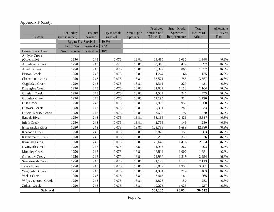
Page 75
Appendix F (cont).
System
Fecundity (per spawner)
Fry per Spawner
Fry to smolt survival
Smolts per Spawner
Predicted Smolt Yield (Model 1)
Smolt Model Spawner
Requirements
Total Return of Adults
Allowable Harvest
Rate Egg to Fry Survival = 19.8% Fry to Smolt Survival = 7.6%
Lower Nass Area Smolt to Adult Survival = 10% Anliyen Creek (Greenville) 1250 248 0.076 18.81 19,480 1,036 1,948 46.8% Ansedagan Creek 1250 248 0.076 18.81 8,919 474 892 46.8% Anudol Creek 1250 248 0.076 18.81 16,322 868 1,632 46.8% Burton Creek 1250 248 0.076 18.81 1,247 66 125 46.8% Chemainuk Creek 1250 248 0.076 18.81 33,571 1,785 3,357 46.8% Cugiladap Creek 1250 248 0.076 18.81 4,311 229 431 46.8% Disangieq Creek 1250 248 0.076 18.81 21,639 1,150 2,164 46.8% Gingietl Creek 1250 248 0.076 18.81 4,529 241 453 46.8% Ginlulak Creek 1250 248 0.076 18.81 17,195 914 1,720 46.8% Gish Creek 1250 248 0.076 18.81 17,998 957 1,800 46.8% Giswatz Creek 1250 248 0.076 18.81 5,331 283 533 46.8% Gitwinksihlkw Creek 1250 248 0.076 18.81 3,698 197 370 46.8% Iknouk River 1250 248 0.076 18.81 53,166 2,826 5,317 46.8% Inieth Creek 1250 248 0.076 18.81 2,796 149 280 46.8% Ishkeenickh River 1250 248 0.076 18.81 125,796 6,688 12,580 46.8% Keazoah Creek 1250 248 0.076 18.81 2,826 150 283 46.8% Ksemamaith River 1250 248 0.076 18.81 6,262 333 626 46.8% Kwiniak Creek 1250 248 0.076 18.81 26,642 1,416 2,664 46.8% Kwinyarh Creek 1250 248 0.076 18.81 4,933 262 493 46.8% Monkley Creek 1250 248 0.076 18.81 18,814 1,000 1,881 46.8% Quilgauw Creek 1250 248 0.076 18.81 22,936 1,219 2,294 46.8% Seaskinnish Creek 1250 248 0.076 18.81 21,128 1,123 2,113 46.8% Tseax River 1250 248 0.076 18.81 36,807 1,957 3,681 46.8% Wegiladap Creek 1250 248 0.076 18.81 4,034 214 403 46.8% Welda Creek 1250 248 0.076 18.81 2,645 141 265 46.8% Wilyayaanooth Creek 1250 248 0.076 18.81 2,826 150 283 46.8% Zolzap Creek 1250 248 0.076 18.81 19,273 1,025 1,927 46.8%
Sub total 505,125 26,854 50,512

Page 76
Appendix F (cont).
System
Fecundity (per spawner)
Fry per Spawner
Fry to smolt survival
Smolts per Spawner
Predicted Smolt Yield (Model 1)
Smolt Model Spawner
Requirements
Total Return of Adults
Allowable Harvest
Rate Egg to Fry Survival = 19.8% Fry to Smolt Survival = 7.6% Smolt to Adult Survival = 10%
Upper Nass Area Bell-Irving River -Above Teigen 1250 248 0.076 18.81 203,316 10,809 20,332 46.8% Bell-Irving River -Bowser to Teigen 1250 248 0.076 18.81 151,510 8,055 15,151 46.8% Bell-Irving River -below Bowser 1250 248 0.076 18.81 83,648 4,447 8,365 46.8% Bowser River 1250 248 0.076 18.81 160,605 8,538 16,061 46.8% Cranberry River 1250 248 0.076 18.81 235,576 12,524 23,558 46.8% Damdochax Creek 1250 248 0.076 18.81 113,844 6,052 11,384 46.8% Hodder Creek 1250 248 0.076 18.81 45,220 2,404 4,522 46.8% Kinskuch River 1250 248 0.076 18.81 156 8 16 46.8% Kiteen River 1250 248 0.076 18.81 129,544 6,887 12,954 46.8% Konigus Creek Kotsinta Creek 1250 248 0.076 18.81 53,889 2,865 5,389 46.8% Kshadin Creek 1250 248 0.076 18.81 414 22 41 46.8% Kwinageese River 1250 248 0.076 18.81 247,348 13,150 24,735 46.8% Kwinatahl River 1250 248 0.076 18.81 20,923 1,112 2,092 46.8% Meziadin River 1250 248 0.076 18.81 187,357 9,960 18,736 46.8% Muskaboo Creek Panorama Creek Paw Creek 1250 248 0.076 18.81 82,607 4,392 8,261 46.8%

Page 77
Appendix F (cont).
System
Fecundity (per
spawner) Fry per
Spawner Fry to smolt
survival Smolts per
Spawner
Predicted Smolt Yield
(Model 1)
Smolt Model Spawner
Requirements
Total Return of
Adults
Allowable Harvest
Rate Egg to Fry Survival = 19.8% Fry to Smolt Survival = 7.6%
Smolt to Adult Survival
= 10%
Upper Nass Area (cont) Saladamis Creek 1250 248 0.076 18.81 38,278 2035 3,828 46.8% Sallysout Creek 1250 248 0.076 18.81 5,331 283 533 46.8% Sanskisoot Creek 1250 248 0.076 18.81 60,623 3,223 6,062 46.8% Sanyam Creek 1250 248 0.076 18.81 1,457 77 146 46.8% Shumal Creek 1250 248 0.076 18.81 36,040 1,916 3,604 46.8% Taft Creek 1250 248 0.076 18.81 93,921 4,993 9,392 46.8% Taylor River Tchitin River 1250 248 0.076 18.81 37,218 1,979 3,722 46.8% Teigen Creek 1250 248 0.076 18.81 116,430 6,190 11,643 46.8% Treaty Creek 1250 248 0.076 18.81 97,030 5,158 9,703 46.8% Upper Nass River Vile Creek 1250 248 0.076 18.81 93,093 4,949 9,309 46.8% White River 1250 248 0.076 18.81 236,623 12,580 23,662 46.8%
Sub total 2,532,001 134,609 253,200