Required Surveillance Performance Accuracy to Support 3 ... · radar systems in depicting the aircraft location and separation between aircraft depends primarily on the range of the

Lincoln LaboratoryMASSACHUSETTS INSTITUTE OF TECHNOLOGY

LEXINGTON, MASSACHUSETTS

Project ReportATC-323

Required Surveillance Performance Accuracy to Support 3-Mile and 5-Mile

Separation in the National Airspace System

S.D. ThompsonJ.W. Andrews

G.S. HarrisK.A. Sinclair

1 November 2006

Prepared for the Federal Aviation Administration,

Washington, D.C. 20591

This document is available to the public through the National Technical Information Service,

Springfield, VA 22161

This document is disseminated under the sponsorship of the Department of Transportation in the interest of information exchange. The United States Government assumes no liability for its contents or use thereof.

17. Key Words 18. Distribution Statement

19. Security Classif. (of this report) 20. Security Classif. (of this page) 21. No. of Pages 22. Price

TECHNICAL REPORT STANDARD TITLE PAGE

1. Report No. 2. Government Accession No. 3. Recipient's Catalog No.

4. Title and Subtitle 5. Report Date

6. Performing Organization Code

7. Author(s) 8. Performing Organization Report No.

9. Performing Organization Name and Address 10. Work Unit No. (TRAIS)

11. Contract or Grant No.

12. Sponsoring Agency Name and Address 13. Type of Report and Period Covered

14. Sponsoring Agency Code

15. Supplementary Notes

16. Abstract

Unclassifi ed Unclassifi ed 120

FORM DOT F 1700.7 (8-72) Reproduction of completed page authorized

S.D. Thompson, J.W. Andrews, G.S. Harris, and K.A. Sinclair

MIT Lincoln Laboratory 244 Wood Street Lexington, MA 02420-9108

This report is based on studies performed at Lincoln Laboratory, a center for research operated by Massachusetts Institute of Technology, under Air Force Contract FA8721-05-C-0002.

This document is available to the public through the National Technical Information Service, Springfi eld, VA 22161.

ATC-323

Required Surveillance Performance Accuracy to Support 3-Mile and 5-Mile Separation in the National Airspace System

Department of Transportation Federal Aviation Administration 800 Independence Ave., S.W. Washington, DC 20591

Project Report

ATC-323

1 November 2006

Surveillance in today’s National Airspace System (NAS) is provided by a system of terminal and en route radars. The separation distance that an air traffi c controller is required to maintain between aircraft depends, in part, on the performance of these radars. The accuracy of these radar systems depends on the range of the aircraft from the radar and whether the aircraft being separated are tracked by the same or different radars. For this reason the separation standards are expressed in terms of range from the radar and also depend on whether or not the two aircraft being separated are tracked by the same or different radars. As new technologies for surveillance are introduced, it is worthwhile to express the requirements for surveillance systems in terms of a technology-independent Required Surveillance Performance (RSP) for the types of separation service being provided, i.e., 3-mile separation or 5-mile separation.

This report presents an analysis and fl ight test validation to derive the RSP accuracy needed to support 3-mile and 5-mile separation. The approach taken in this analysis is to examine the error characteristics of the various types of surveillance sensors in the FAA inventory and to analyze their performance with regard to providing accurate separation measurements to controllers. The report is organized to fi rst give a background describing the current surveillance systems and separation standards and their evolution. Next the concept of RSP is introduced. This is followed by a section describing the analysis that was used to derive the RSP attributes presented in this paper followed by a description and results of a fl ight test performed to validate this analysis.

Required Surveillance Performance, RSP, Air Traffi c Control

iii

EXECUTIVE SUMMARY

The Federal Aviation Administration is modernizing the Air Traffic Control system to improve flight efficiency, to increase capacity, to reduce flight delays, and to control operating costs as the demand for air travel continues to grow. Promising new surveillance technologies such as Automatic Dependent Surveillance Broadcast, (ADS-B), multisensor track fusion, and multifunction phased array radar offer the potential for increased efficiency in the National Airspace System (NAS). However, the introduction of these surveillance systems into the NAS is hampered because the FAA Order containing the surveillance requirements to support separation services assumes surveillance is provided by radar technology. The requirements are stated in terms that don’t apply to new surveillance technologies. In order to take advantage of new surveillance technologies, the surveillance requirements to support separation services in the NAS must be articulated from a performance perspective that is not technology specific. This will allow the FAA to make the investment and performance trade-off analysis necessary to support the introduction of new surveillance technologies.

Historically, requirements for the performance of new surveillance systems have been based on the assumption that these systems performed in a similar manner to the existing rotating secondary and primary radar systems. This is not the case for many new proposed surveillance technologies and a fundamental change in concept for the method of approving such systems is needed. Consequently, international standardization is increasingly based on Required Total System Performance (RTSP) specifications that are independent of the particular technology or implementation that is used to support a service. The term Required Surveillance Performance (RSP) is the subset of RTSP that is concerned with the surveillance requirements needed to support various services. This report is concerned with the accuracy attributes of RSP to support 3-mile and 5-mile separation services. The establishment of an RSP will facilitate the approval of newer surveillance technologies that may provide faster and more accurate position reports but do not now have any basis for seeking approval.

RSP consists of more than the accuracy of the surveillance system although that is the primary focus of this analysis. The approach taken in this report is to base the RSP accuracy and latency on analysis and flight test results. Other applicable RSP attributes must reference the specifications for existing acceptable legacy systems. The RSP attributes adopted in ongoing work by the ICAO Surveillance and Conflict Resolution Systems Panel (SCRSP) working groups include availability, continuity of service, and integrity. This is a work in progress and papers that can be referenced are not yet available but at least a sub-set of the attributes being considered are available in the specifications for existing systems.

This report takes the reference system approach; one of two approaches recognized by the International Civil Aviation Organization (ICAO). In the reference system approach a new concept for providing a service is compared to a reference system that is already proven to safely and satisfactorily

iv

provide that service. The reference system approach is generally faster and thus less expensive than the alternative, a Target Level of Safety approach, and has the advantage of testing against a similar system with a proven safety record.

Surveillance in today’s National Airspace System (NAS) is provided by a system of terminal and en route track-while-scan radars. The separation distance that an air traffic controller is required to maintain between aircraft depends, in part, on the performance of these systems. The accuracy of these radar systems in depicting the aircraft location and separation between aircraft depends primarily on the range of the aircraft from the radar antenna and whether the aircraft are being tracked by the same or different radar sensors. For that reason, the separation standards are defined in these terms. The current separation standards are contained in FAA Order 7110.65 and they require that aircraft be separated horizontally by radar if the altitude between the aircraft is less than one thousand feet. The separation between aircraft must be at least five nautical miles unless both aircraft are within 40 miles of the radar antenna and are being tracked by the same radar; in that case the separation can be reduced to three nautical miles. The Order does not differentiate between different types of radar that may have different performance. In addition, there are no provisions for technologies different than radar.

There are at least two new technologies currently under consideration for providing surveillance in the NAS; Automatic Dependent Surveillance Broadcast (ADS-B) and multisensor track fusion. Under the ADS-B concept, aircraft automatically broadcast a state vector once per second that include the aircraft position, velocity, identity, intent, and emergency status. A key advantage of this approach is that surveillance can be achieved through low-cost, listen-only ground stations. The position accuracy becomes dependent upon the source avionics, typically a Global Positioning System (GPS) receiver, and not on the range of the aircraft from the listen-only ground station. The average time interval between position updates for an ADS-B equipped aircraft is shorter than for terminal radar which completes a rotation every 4.8 seconds. However, the ADS-B reports for different aircraft are uncorrelated while the updates from radar occur almost simultaneously for aircraft separated by only three miles. In addition, there will necessarily be a transition period where some aircraft are under radar surveillance and some may be reporting position through ADS-B. Separation requirements for a mixed system are not addressed by the current separation standards.

The multisensor track fusion approach uses position reports from multiple radars and a fusion tracker to optimize the position reports and synchronize the display for aircraft separation. Under FAA Order 7110.65, multisensor track fusion would not be approved for 3-mile separation because the aircraft are not being tracked by a single sensor.

There are two fundamentally different ways that azimuth measurements are made with the radar beacon systems that are in the FAA’s inventory today. The older “sliding window” system sends out multiple interrogations across the beam width (typically 16 across the two and one half degree beam width) and measures the azimuth as the center of the multiple replies from the aircraft’s transponder. This method is subject to garble from the replies from other aircraft that can interfere with the identification of the edges of the beam width or even split the replies into two apparent targets. These

v

systems have been in the inventory for decades and have provided safe 3-mile separation services in the terminal area and 5-mile separation in en route airspace. Newer Monopulse Secondary Surveillance Radar (MSSR) sensors use multiple beam patterns for interrogations that provide an azimuth measurement from a single transponder reply. This system has proven more accurate and less susceptible to interference from other aircraft.

When collocated secondary and primary radars both make a range and azimuth measurement to the same target the measurement is said to be reinforced; a site-selectable parameter determines which of the two reports is sent from the radar to the facility for a reinforced target. In general, it is the primary radar measurement of range and azimuth that is reported for reinforced targets at radars having sliding window beacon sensors collocated with the primary radar and the beacon measurement for MSSR sensors collocated with primary radars. The primary performance is slightly better than the sliding window performance and not as good as the MSSR performance. However, clutter and interference such as from weather can degrade the primary performance to the point that it is the sliding window beacon only report that is used to provide 3-mile and 5-mile separation service. In addition, some sites are beacon only and at some sites the sliding window measurement has been selected for reporting of reinforced targets. For these reasons, the performance of the terminal sliding window sensor at a range of 40 miles was chosen as the reference system for 3-mile separation and the en route sliding window sensor at a range of 200 miles for 5-mile separation. Aircraft speeds are limited to 250 knots below 10,000 feet altitude where 3-mile separation is normally provided and so the aircraft were assumed to have velocities of 250 knots for 3-mile separation and 600 knots for 5-mile separation.

The beacon radar performance was modeled using a Monte Carlo simulation of the various error sources based on specifications and field test performance measurements of operating sensors in the field. The accuracy metrics for RSP were absolute geographic position accuracy and accuracy in measured separation between two aircraft three miles and five miles in-trail.

The modeled performance was validated through a flight test of two aircraft flying three-miles in-trail in Boston ARTCC airspace and recording true position with on-board GPS units. Sensor data from all sensors reporting the position of the aircraft to the Boston facility was recorded as well as the recording of data used to generate the display on the controller’s scope.

The result of this analysis and flight test verification is a set of accuracy, latency, and update rate requirements for 3-mile and 5-mile separation service shown in the following tables. These requirements represent limits on the total errors displayed to a controller and include any errors introduced between the surveillance sensor and the display.

vi

Required Accuracy, Latency, and Update Rate for 3-NM Separation

Required Accuracy, Latency, and Update Rate for 5-NM Separation

Geographical Position Accuracy σ < 0.20 NM

Accuracy in Measured Separation

Standard Deviation σ < 0.16 NM

No more than 10 % of the error distribution shall exceed ± 0.28 NM


No more than 0.1 % of the error distribution shall exceed ± 0.65 NM

Latency 2.2 seconds to display maximum

Update Rate 4.8 seconds maximum








Update Rate 12 seconds maximum

vii

It is important to note that the reference system approach results in an RSP that represents a “sufficient” rather than “necessary” level of performance. That is, if the performance level of all attributes of the RSP is met, the surveillance system performance will be sufficient to support the 3-mile or 5-mile separation service. However, it may be that satisfactory performance can be met even if one or more attributes do not meet the RSP requirements. This must be validated through trade-off studies with other attributes or by operational considerations. A candidate surveillance technology that met or exceeded each attribute described in the tables would provide surveillance accuracy at least as good as that which is used to support 3-mile and 5-mile separation services. However, a candidate system that provided far greater geographic accuracy and met the accuracy in measured separation requirement might be acceptable even if the update rate occasionally exceeded the 4.8 second requirement.

ix

TABLE OF CONTENTS

Page

Executive Summary iii List of Illustrations xi List of Tables xvii

1. INTRODUCTION 1

2. BACKGROUND 3

3. RADAR SEPARATION STANDARDS 7

3.1 Origin of Standards 7 3.2 Current Standards 7 3.3 Role of Surveillance in Separation Requirements 8

4. REQUIRED SURVEILLANCE PERFORMANCE 13

5. ANALYSIS 15

5.1 Technical Approach 15 5.2 Error Characteristics of Secondary Radar Sensors 20 5.3 Reporting and Error Characteristics of Surveillance Systems that Include

Primary Radars 23 5.4 Errors in Measured Separation from Independent Surveillance Systems 25 5.5 Required Surveillance Performance Accuracy Metric 25 5.6 Monte Carlo Analysis of Sensor Errors 26 5.7 Display System Processing Errors 35 5.8 Total System Errors to the Display 41

6. FLIGHT TEST VALIDATION 45

6.1 Purpose 45 6.2 Data Recording 45 6.3 Flight Path 50

x

TABLE OF CONTENTS (CONTINUED)

Page 6.4 Flight Test Simulation 50 6.5 Flight Test Results 51

7. STATEMENT OF REQUIRED SURVEILLANCE PERFORMANCE 93

7.1 Selection of RSP 93 7.2 3-NM Separation Requirements 94 7.3 5-NM Separation Requirements 95

8. SUMMARY AND CONCLUSIONS 97

List of Acronyms 99

References 101

xi

LIST OF ILLUSTRATIONS

Figure Page No.

1 Role of surveillance in separation standards. 9 2 Comparison of reference case and new case at the p < 0.001 point. 11 3 The relative position of route structures and the region of degraded surveillance

performance may make the separation task more difficult for the reference case. 14 4 Data flow for derivation of required surveillance performance. 19 5 Comparison of sliding window and monopulse azimuth measurement techniques. 21

6 Geometry for sensor error modeling for 3-NM separation. 27

7 Sensor separation estimate errors for a single ATCRBS sliding window short-range

radar at a range of 40 miles and aircraft velocities of 250 knots. 28 8 Sensor separation estimate errors for a single primary short-range radar at a range

of 40 miles and aircraft velocities of 250 knots with little or no rain or clutter. 29

9 Sensor separation estimate errors for a single MSSR short-range radar at a range of 60 miles and aircraft velocities of 250 knots. 30

10 Geometry for sensor error modeling for 5-NM separation. 32 11 Separation estimate errors for single sensor long-range ATCRBS sliding window

sensor at a range of 200 miles and aircraft velocities of 600 knots. 33 12 Separation estimate errors for single sensor long-range MSSR sensor at a range of

200 miles and aircraft velocities of 600 knots. 34 13 Sample tracks of two aircraft from the RADES data being tracked by the Stewart

radar at Boston ARTCC. 37

xii

LIST OF ILLUSTRATIONS (CONT.)

Figure Page No.

14 Comparison of measured separation versus time from the RADES data and

the SAR data for a sample case. 38 15 Typical histogram of difference between sensor measurement of separation in the

RADES data and displayed separation in the SAR data. Fifty cases were summed to measure display system processing error. 39

16 Histogram of HOST display system processing errors for single sensor measured from 39 sample cases of aircraft pairs recorded at Boston ARTCC on October 6, 2004. 40

17 Histogram of HOST display system processing errors for multiple sensors

measured from 39 sample cases of aircraft pairs recorded at Boston ARTCC on October 6, 2004. 41

18 Total system error for long-range sliding window sensor at 200 mile range with

single sensor HOST system display processing. 42 19 Total system error for long-range MSSR system at 200 mile range and aircraft at

600 knots with HOST system display processing for a single sensor. 43 20 Ashtech Model GG24 GPS plus Glonass sensor. 45 21 Falcon 20 lead aircraft in flight test. 46 22 Gulfstream G2 trailing aircraft in flight test. 47 23 Typical RADES screenshot of flight paths of all aircraft being tracked by all sensors. 48 24 RADES data viewer sample screen. 49 25 Flight tracks from radar data (RADES) and location of sensors. 51

xiii


Figure Page No.

26 Radar hits of flight test aircraft recorded by RADES during the flight test. 52 27 Position data generated by the simulation over a portion of the flight test path

for the Falcon. 53 28 Position data measured by RADES over a portion of the flight test path for the Falcon. 54 29 Position data generated by the simulation over a portion of the flight test path

for the Gulfstream. 55

30 Position data measured by RADES over a portion of the flight test path for the Gulfstream. 56

31 Flight tracks from GPS for Falcon and Gulfstream. 57 32 Gulfstream latitude measurements from GPS and time corrected RADES,

all tracking sensors. 58

33 Gulfstream latitude measurements from GPS and time corrected RADES, all tracking sensors, enlargement of Turn 1. 59

34 Gulfstream latitude measurements from GPS and time corrected RADES, all tracking sensors, enlargement of Turn 2. 60

35 Gulfstream latitude measurements from GPS and time corrected RADES,

all tracking sensors, enlargement of Turn 3. 61 36 Earth centered, Earth fixed GPS position of Falcon. 62

37 Earth centered, Earth fixed GPS position data for Gulfstream. 63

38 Separation between the Falcon and Gulfstream during the flight versus time

(GPS data). 64

xiv


Figure Page No.

39 Separation between the Falcon and Gulfstream during the flight test portion of the

flight versus time (GPS data). 65

40 Range from the Hartford radar (QHA) site to the mid-point between the two flight test aircraft as a function of time. 66

41 Example of update delta times versus time for the Hartford radar (QHA) tracking

both flight test aircraft. 67 42 Position reports of the flight test aircraft during continuous tracking of both aircraft

by the Hartford radar (QHA). 68

43 Separation of the flight test aircraft as a function of time as measured by the Hartford radar (QHA). 69

44 Sampled measurements of the separation of the aircraft by the Hartford radar (QHA). 70

45 Modeled error limits versus range for MSSR sensors. 71

46 Modeled error limits versus range for sliding window sensors. 72 47 Modeled error limits versus range for MSSR sensors with expanded scale. 73

48 Theta error measurements on both flight test aircraft as a function of time for the

Remson radar (QXU), a long-range sliding window sensor. 75

49 Curve fitting of the Remson (QXU) theta error data. 76 50 Separation of the azimuth error (θ) into azimuth bias and jitter for the Remson

(QXU) long-range sliding window sensor. 77

51 Theta error measurements on both flight test aircraft as a function of time for the Bradley radar (BDL), a short-range MSSR sensor. 78

52 Curve fitting of the Bradley (BDL) theta error data. 79

xv


Figure Page No.

53 Separation of the azimuth error (θ) into azimuth bias and jitter for the Bradley

(BDL) short-range MSSR sensor. 80

54 Theta error measurements on both flight test aircraft as a function of time for the Hartford radar (QHA), an MSSR sensor exhibiting a discontinuity in the bias as the aircraft passed near the sensor. 81

55 Standard deviation (σ) of azimuth jitter errors for the nine sensors recording both flight test aircraft; errors for sliding window sensors compared to MSSR sensors. 82

56 Distribution of azimuth jitter errors for all MSSR sensors. 83

57 Distribution of azimuth jitter errors for all sliding window sensors. 84 58 Distribution of azimuth bias errors for all sensors. 86

59 Diagram showing the relationship between clock bias, latency, and time offset. 87 60 Example of RADES versus GPS data used to compute time offset. 88

61 Example of SAR versus GPS data used to calculate absolute latency. 89 62 Illustration showing the relationship between Δt and Δx. 90

xvi

xvii

LIST OF TABLES

Table Page No.

1 Summary of Cases Analyzed for 3-mile and 5-mile Separation RSP 17 2 Error Sources Used in Monte Carlo Simulations for Beacon Sensors 22 3 Sensor Error Sources Used in Monte Carlo Simulations for Primary Sensors 24 4 Sensor Measured Separation Error Distribution Characterization for Beacon and

Primary Sensors for 3-NM Separation 31 5 Sensor Measured Separation Error Distribution Characterization for Beacon

Sensor Errors for 5-NM Separation 35

6 Total System Measured Separation Error Distribution Characteristics for 5-NM Separation Cases 44

7 Summary of Latency Results for RADES and SAR Data 91 8 Required Accuracy, Latency, and Update Rate for 3-NM Separation 94

9 Required Accuracy, Latency, and Update Rate for 5-NM Separation 95

1

1. INTRODUCTION

Surveillance in today’s U.S. National Airspace System (NAS) is provided by a system of terminal and en route radars. The separation distance that an air traffic controller is required to maintain between aircraft depends, in part, on the performance of these radars. The accuracy of these radar systems is range dependent and also different depending on whether the aircraft are being tracked by the same or different radars. For this reason the separation standards are expressed in terms of range from the radar and differ if the aircraft being separated are not tracked by the same radar. As new technologies for surveillance are introduced, it is worthwhile to express the requirements for surveillance systems in terms of a technology-independent Required Surveillance Performance (RSP) for the types of separation service being provided, i.e., 3-mile separation as is typically provided in the terminal area or 5-mile separation typically provided in en route airspace. This is analogous to the Required Navigation Performance (RNP) requirements that have been derived for various navigation services such as en route navigation or precision instrument landing guidance.

Historically, requirements for the performance of new surveillance systems have been based on the assumption that these systems performed in a similar manner to the existing rotating secondary and primary radar systems. This is not the case for many new proposed surveillance technologies and a fundamental change in concept for the method of approving such systems is needed. Consequently, international standardization is increasingly based on Required Total System Performance (RTSP) specifications that are independent of the particular technology or implementation that is used to support a service. The term Required Surveillance Performance (RSP) is the subset of RTSP that is concerned with the surveillance requirements needed to support various services1,2. This report is concerned with the RSP to support 3-mile and 5-mile separation services. The establishment of an RSP will facilitate the approval of newer surveillance technologies that may provide faster and more accurate position reports but do not now have any basis for seeking approval because they employ technologies different from radars.

This report presents an analysis and flight test validation to derive the RSP accuracy to support 3-mile and 5-mile separation. The analysis examines the error characteristics of the various types of surveillance sensors in the FAA inventory and analyzes their performance with regard to providing accurate separation measurements to controllers. The RSP is then established based on the acceptable performance of existing systems in wide-spread use that have safely supported air traffic separation services. This approach taken to establishing the RSP is termed a reference system approach, one of two approaches recognized by the International Civil Aviation Organization (ICAO). In the reference system approach the requirements for providing a service are based on a reference system that has proven to safely and satisfactorily support that service. The other approach, Target Level of Safety, is based on analysis that attempts to prove the absolute safety of an alternate technology and prove that it fits within an allowed safety budget. This is a more involved approach and is considered more

2

appropriate for new services. A reference system approach has the advantage of basing requirements on a system with a proven safety record.

Two cases are analyzed for comparison for both 3-mile and 5-mile separation; 1) an RSP case based on systems that have been in widespread use providing 3-mile and 5-mile separation safely across the NAS, and 2) a current technology case representative of systems currently being procured. The objective of this analysis is to establish a single RSP for all facilities providing 3-mile and 5-mile separation, so the RSP case mentioned previously is used as the basis for defining RSP.

In the future, it may be necessary to generate an RSP based on the Target Level of Safety approach. Such an assessment must consider performance under a variety of faults as well as under nominal operating conditions. This is clearly much more involved than a reference system approach, and the modeling and data validation required may be infeasible for near-term results. Fortunately, the key issue of 3-mile versus 5-mile separation does not require such complete modeling. By assuming that fault modes are handled in the same manner with both standards, we can argue that the RSP can be based on equivalent performance. Note that if the comparison involves surveillance systems with greatly different types of faults, then it will be necessary to take particular system faults into account3.

This report is organized to first give a background describing the current surveillance systems and separation standards and their evolution. Next the concept of RSP is introduced. This is followed by a section describing the analysis that was used to derive the RSP presented in this report followed by a description and results of a flight test performed to validate this analysis.

3

2. BACKGROUND

Before the introduction of radar, pilots either accepted responsibility for visual separation or procedural separation was used by air traffic controllers to maintain safe distances between aircraft. In procedural separation, blocks of airspace are reserved for one airplane at a time. Position reports are provided by the pilots to the controllers, who then provide separation by clearing only one aircraft at a time into a of block airspace. Procedural separation is still used in the NAS today in areas without radar coverage or where operationally advantageous.

With the introduction of radar, separation standards were introduced based on the performance of these early radar sensors. The first radars used in air traffic control used the primary return (the electromagnetic reflection from the skin of the airplane) displayed on the scope to separate aircraft. Because errors in azimuth measurement result in increased position errors as the range of the aircraft increases from the radar, separation standards were introduced that are a function of how far the aircraft are from the radar. There was no specific analysis done to justify the original separation requirements (see Section 3.1), however, the standards proved safe and effective in the airspace of that day. The standards were refined as the radar equipment accuracy and range were improved but they have remained relatively constant over the last several decades.

The introduction of secondary or beacon radar offered a significant improvement in the performance of radar sensors by utilizing the reply from an aircraft’s transponder for measuring position. The use of a transponder allows for a higher power return and allows the aircraft to supply the system with data such as aircraft identification and altitude. Today’s radars are a surveillance system comprising a primary radar, a secondary radar, and software for combining reports and for identifying individual aircraft paths or “tracks.” A target report that merges both a primary and secondary measurement is called a “reinforced” report.

Older surveillance systems use secondary radar systems known as “sliding window” Air Traffic Control Radar Beacon System (ATCRBS) sensors. These sensors utilize replies from the aircraft’s transponder across the entire beam width to make an azimuth estimate of the aircraft’s position. Examples include systems that employ the Beacon Interrogator 5. Newer Monopulse Secondary Surveillance Radar (MSSR) systems (e.g., Beacon Interrogator 6, Mode S) make an azimuth measurement for every transponder reply and are replacing the older sliding window sensors in both the terminal and en route domains. A more detailed explanation of the operation of these systems is contained in Section 5.2 of this document which describes the error characteristics of secondary sensors applied in this analysis.

The automation systems that accepts the combined data from the primary and secondary sensors and determines which reports are assigned to a track for a given aircraft on a specific display will be referred to as “display system processing” in this report. There are a number of different display

4

system processing packages that are in use in the NAS, each with different characteristics. Regardless of the display processing system in use, the position measurement of the system that is displayed to the controller is, for the vast majority of the reports, the position estimate from the secondary (beacon) radar for facilities equipped with monopulse beacon systems, even though both beacon and primary measurements are taken. When the primary radar is collocated with a sliding window secondary surveillance system, the position information for a merged target is generally the position estimate made by the primary radar. However, clutter and interference such as from weather can degrade the primary performance to the point that it is the sliding window “beacon only” report that is used to provide three-mile and five-mile separation service. In addition, some sites are “beacon only” and at some sites the sliding window measurement has been selected for reporting of reinforced targets.

Sliding window secondary surveillance beacon systems have been in use for many years at busy terminals and at en route Air Route Traffic Control Centers safely providing three-mile and five-mile separation. Although these systems are being replaced with monopulse systems throughout the NAS, the sliding window beacon system is considered the baseline requirement for separation performance.

Thompson and Bussolari4 reviewed the error characteristics of long-range and short-range sliding-window ATCRBS and MSSR surveillance sensors. Errors in the measured separation distance between targets were analyzed for both single sensor and mosaic cases. Monte Carlo simulations were run to compute the errors in measured separation as a function of range from the sensor. The display system processing was explicitly excluded from the analysis so that the sensor errors could be directly compared and because the separation standards in use are independent of the display system processing used.

MSSR sensors were found to offer an approximately three-fold increase in azimuth accuracy over sliding-window ATCRBS sensors. The MSSR sensors were found to provide equivalent separation performance at a range of over 100 miles compared to the ATCRBS sliding window performance at a 40-mile range. Multiple MSSR sensors in a mosaic display also offer separation performance equivalent to a single sliding-window ATCRBS sensor when each aircraft is within 40 miles of its respective sensor.

An extension of this analysis technique is employed to derive RSP based on the existing acceptable performance of legacy systems comprising both primary and secondary radars. In addition to sensor errors, errors in representative display system processing are considered so that the RSP limits represent the total allowable error between the true separation of aircraft and the separation displayed to a controller on the scope.

RSP consists of more than the accuracy of the surveillance system although that is the primary focus of this analysis. The approach taken in this report is to base the RSP accuracy and latency on analysis and flight test results. Other applicable RSP attributes must reference the specifications for existing acceptable legacy systems. The RSP attributes adopted in ongoing work by the ICAO Surveillance and Conflict Resolution Systems Panel (SCRSP) working groups include availability,

5

continuity of service, and integrity. This is a work in progress and papers that can be referenced are not yet available but at least a sub-set of the attributes being considered are available in the specifications for existing systems.

6

7

3. RADAR SEPARATION STANDARDS

3.1 ORIGIN OF STANDARDS

A history of the origins of the initial radar separation standards for civil air traffic control is given by FAA Agency historian Preston5. Preston notes that the establishment of the separation standards “...was the result of an evolutionary process that included close coordination with airspace users.” and that the standard “...represented a consensus of the aviation community.” It is clear that no specific analytical approach was used to derive the separation standards and there are, according to Preston, different accounts of how the specific standards were chosen. The separation standard for terminal procedures was set at 3 miles and for en route at 5 miles. Preston concluded that the basis for setting the standards “...seems to have included such factors as: military precedent; reasoned calculations; a desire to choose a figure acceptable to pilots; and the limitations of both the radar equipment and of the human elements of the system. The use of 5 miles as the separation for flights over 40 miles from the radar site was based on the greater limitations of the long-range equipment.”

The original standards were set at a time when only primary radar was available and the traffic was considerably slower and less dense than in today’s airspace. The airspace and surveillance equipment are much different today and efforts to derive an RSP based on what existed when the separation standards were originally instituted is baseless.

3.2 CURRENT STANDARDS

In Air Traffic Control, range and separation “miles” always means nautical miles and that is the convention continued throughout this report. The abbreviation used to represent nautical miles is NM. Radar separation standards are conveyed in FAA Order 7110.65N6. The order allows 3-mile separation between aircraft as long as both aircraft are less than 40 miles from and tracked by the same sensor antenna, otherwise the traffic must be separated by five miles. A separation of three miles is not permitted with a mosaic display (described below); 5-mile separation is required. The order makes no distinction in separation requirements based on the performance of the radar, and applies equally to short- and long-range radars.

In a mosaic display, the airspace is divided into geographical areas called radar sort boxes and each sort box is assigned a preferred sensor and supplemental and tertiary sensors. As long as the preferred sensor is measuring the aircraft position, the position reported by that sensor is displayed to the controller. Typically, contiguous sort boxes are assigned to the same preferred sensor and there are boundaries between geographical areas being covered by a preferred sensor. These boundaries, in general, will not correspond to sector boundaries. When aircraft separated by a controller fall into different coverage areas, different sensors will report the aircraft positions. In addition, a controller

8

will not necessarily know when coverage is lost by a preferred sensor and the position report is being provided by a supplemental sensor. In a mosaic environment it is possible for two aircraft being separated to have their position estimates provided by different radars, thus 3-mile separation is not currently allowed in a mosaic environment. If there is a significant operational advantage to be obtained by modifying a radar site adaptation so that a particular control area can only be served by a single radar (known as “single site adaptation”) then the separation can be reduced to 3 miles in en route airspace when both aircraft are within 40 miles of that sensor and operating below Flight Level 180 (18,000 feet altitude with standard day pressure setting).

En Route Air Route Traffic Control Centers (ARTCCs) generally operate in a mosaic display mode and provide 5-mile separation. Individual Terminal Radar Approach Control (TRACON) facilities generally operate in single-site mode and provide 3-mile separation. If there are multiple radars in use at a TRACON each of the radars has historically been adapted so that only reports from a single radar will go to the display responsible for the designated airspace in such a manner that an individual controller will always be separating traffic based on a single sensor.

The new consolidated TRACONs being introduced by the FAA will have the capability to employ a mosaic display across their airspace. Sort boxes in mosaic displays at Air Route Traffic Control Centers are large, 16 miles by 16 miles, but the mosaic displays being considered at some consolidated TRACONs may use much smaller 1-mile by 1-mile sort boxes. Additionally, some Centers are now choosing to convert some of their sort boxes to single site adaptation so they can permit 3-mile separation in portions of their airspace.

The separation standards represent the minimum allowable separation between aircraft. It is important to note that there is no requirement for air traffic controllers to separate traffic to the minimum separation standard. In the ARTCCs there is an alarm that will sound if the 5-mile separation is violated.

3.3 ROLE OF SURVEILLANCE IN SEPARATION REQUIREMENTS

Although surveillance is an important factor in determining separation standards, it is not the only factor as illustrated in Figure 1. Consequently, any safety analysis comparing the separation measurement accuracy of different surveillance systems must hold the other factors affecting separation constant. In other words, the performance of the systems must be compared in the same and current environment. The approach taken in this analysis is to determine the required surveillance performance for the existing separation standards in the existing environment. This is in contrast to a target level of safety approach that must model the entire system illustrated in Figure 1. It is not valid to apply the target level of safety requirement to a model limited to the surveillance element. Doing so would potentially allow separation procedures not supportable by the performance of the other elements.

9

Figure 1. Role of surveillance in separation standards.

For example, an analysis of a theoretically “perfect” surveillance system that models only

surveillance accuracy against a target level of safety would indicate that existing separation standards could be reduced to near zero. But this would not be supported by other elements that contribute to how far aircraft can move towards each other and be safely separated. The factors illustrated above include time (command and control latency) and relative velocity (airspeed and relative geometry).

The command and control loop between the controllers and the aircraft will affect separation. Air traffic controllers provide the required separation by issuing clearances including routings, vectors (headings), and altitude assignments. This is accomplished through a voice channel (VHF for civilian, or UHF for the military) with a common channel being assigned to a given airspace. High Frequency (HF) and data link are used to communicate with oceanic traffic. Communications between the controller and pilots is subject to interference when more than one person attempts to speak at the same time. There is also opportunity for misunderstanding because of less than perfect reception or because

10

of human error. Enough separation must be provided to allow for latencies in controller clearances being executed.

Airspeed is an obvious element to separation standards; aircraft in the terminal area where 3-mile separation is provided are normally limited to 250 knots indicated airspeed while aircraft in the en route environment may have ground speeds over 600 knots.

The relative geometry of the aircraft will depend on the air traffic operations such as the traffic flow patterns. For instance, it may be easier for a controller to provide separation to an incoming stream of arriving traffic in-trail at the same airspeed, but more difficult to provide separation to crossing traffic or traffic that is climbing or descending relative to other traffic.

A surveillance system that was safe and adequate to provide 3-mile separation to a few DC-3’s arriving in a line to Washington’s National Airport could not handle the terminal jet traffic in the Capitol region today. Therefore when comparing the performance of one surveillance system relative to another, it is import to do so in the same air traffic control environment.

Any analysis that seeks to determine equivalent performance between two surveillance systems is made simpler if it can be assumed that a number of factors that might influence performance are the same and therefore do not have to be explicitly analyzed. An assessment based on determining the absolute level of safety would require consideration of all factors affecting the level of safety. But by employing a relative performance assessment we are able to examine the differences between two systems and thus establish equivalency of performance between a legacy system and a new system.

Figure 2 illustrates the approach used in comparing the reference case with the new case. The legacy case has a certain error distribution out to some moderate cutoff point (shown in this example as the point at which the probability is 0.001 for a data point lying at a smaller value). The assertion of equivalency depends upon the following

1) The critical point (p < 0.001) for the new case is to the right of the same point for the reference case.

2) The faults that can produce points in the tail of the distribution are no worse for the new case than for the reference case.

Item 1 can be verified by data analysis and modeling based on performance specifications. Item 2 must be based on both expert engineering judgment and a limited assessment of possible faults. When the systems being compared are similar in terms of technology, the assertion that they have similar faults gains credibility.

11

Figure 2. Comparison of reference case and new case at the p < 0.001 point.

12

13

4. REQUIRED SURVEILLANCE PERFORMANCE

The FAA has a goal expressed in its Operational Evolution Plan7 and FAA Flight Plan8 to increase capacity and reduce constraints in the National Airspace System. One area that might provide benefits is increasing the airspace in which 3-mile separation is approved. The FAA, based in part on an analysis of the performance of newer monopulse secondary systems4, has recently issued approval to extend the range from a single-site sensor for which 3-mile separation is approved from 40 miles to 60 miles for ASR-9 with Monopulse sensors. This extension was implemented with no software change to the radar but only required a change to FAA Order 7110.65. An extension past 60 miles would have required a software change as current terminal systems do not report targets beyond 60 miles.

A natural extension to this approach is to define the Required Surveillance Performance (RSP) for which any technology can be used to provide the currently approved 3-mile and 5-mile separation. This RSP should be based on existing legacy systems for which 3-mile and 5-mile separation is provided but will allow surveillance systems based on new technologies other than radar to prove that they can provide acceptable service. This offers the potential of further increasing the airspace in which 3-mile separation is approved and of allowing 5-mile separation using alternative surveillance techniques such as Automatic Dependent Surveillance-Broadcast (ADS-B) in airspace where radar coverage is unavailable.

In addition, an unambiguous standard, independent of a given technology, will facilitate potentially new uses of legacy equipment such as surveillance fusion. As new technologies are introduced and improvements to existing technologies are made, an RSP, based on service performance required and not on a given sensor type, remains a consistent standard by which innovative technologies and techniques can be compared and approved for use in the NAS. The separation standards and FAA Order 7110.65 need not be updated with each additional sensor improvement.

There is a recent precedence to this approach taken in the field of navigation. The navigation performance requirements historically have been based on fielded equipment such as the Very High Frequency (VHF) Omni-directional Range (VOR) for en route navigation and the Instrument Landing System (ILS) for precision landing guidance. Now, the Required Navigation Performance (RNP) sets requirements for services and allows any new technology to provide that service if it meets the requirements. This has facilitated the benefits from the introduction of Global Positioning System (GPS) into the National Airspace System.

Establishing a single RSP accuracy requirement for a particular aircraft separation (either 3 or 5 NM) in all airspace may require consideration of the difference between area-wide and localized performance. An illustration of this consideration is provided in Figure 3. The reference case shows a

14

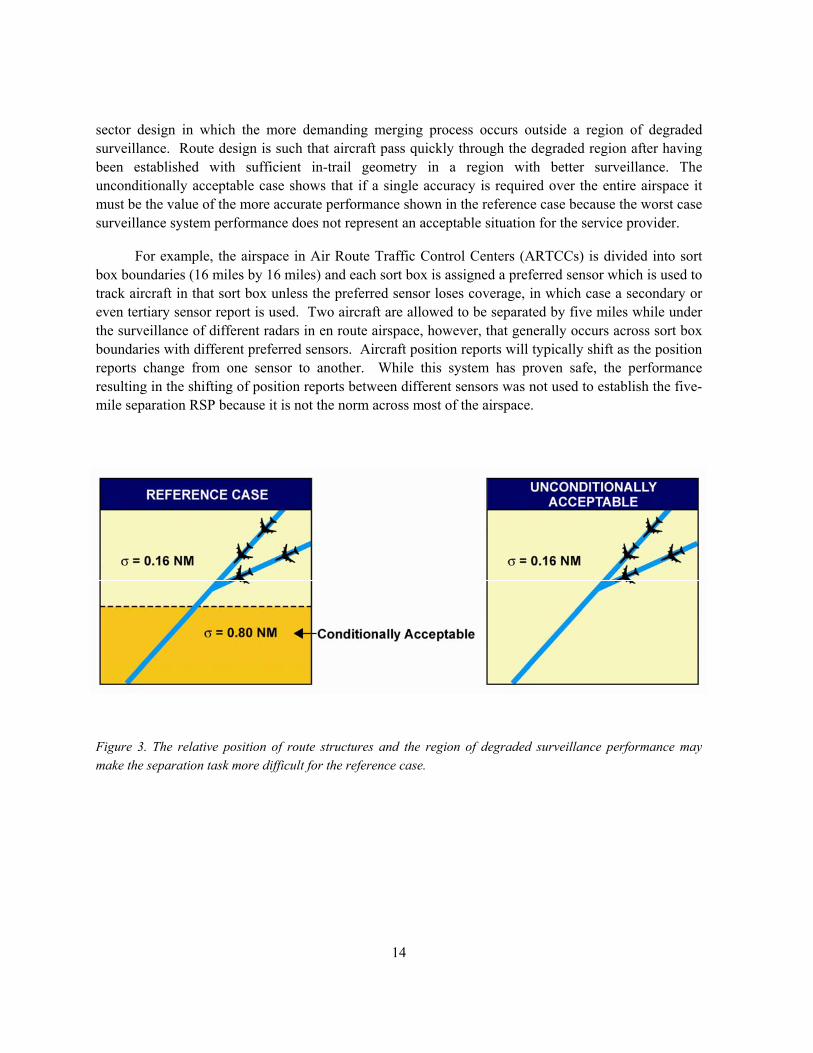
sector design in which the more demanding merging process occurs outside a region of degraded surveillance. Route design is such that aircraft pass quickly through the degraded region after having been established with sufficient in-trail geometry in a region with better surveillance. The unconditionally acceptable case shows that if a single accuracy is required over the entire airspace it must be the value of the more accurate performance shown in the reference case because the worst case surveillance system performance does not represent an acceptable situation for the service provider.

For example, the airspace in Air Route Traffic Control Centers (ARTCCs) is divided into sort box boundaries (16 miles by 16 miles) and each sort box is assigned a preferred sensor which is used to track aircraft in that sort box unless the preferred sensor loses coverage, in which case a secondary or even tertiary sensor report is used. Two aircraft are allowed to be separated by five miles while under the surveillance of different radars in en route airspace, however, that generally occurs across sort box boundaries with different preferred sensors. Aircraft position reports will typically shift as the position reports change from one sensor to another. While this system has proven safe, the performance resulting in the shifting of position reports between different sensors was not used to establish the five-mile separation RSP because it is not the norm across most of the airspace.

Figure 3. The relative position of route structures and the region of degraded surveillance performance may make the separation task more difficult for the reference case.

15

5. ANALYSIS

5.1 TECHNICAL APPROACH

The technical approach taken in this report is to base the Required Surveillance Performance on legacy surveillance systems in widespread use that are acceptable to the controllers for providing 3-mile and 5-mile separation. The least restrictive unconditionally acceptable systems in widespread use are compared with the newer systems being introduced to examine the difference in performance before establishing the accuracy requirement for RSP. The rationale is that currently acceptable systems have consistently been proven to provide the surveillance performance necessary to support the required service. The analysis of the newer systems currently being procured allows a comparison to this baseline. Two cases are analyzed for both 3-mile and 5-mile separation; 1) an RSP model based on systems that have been in widespread use providing 3-mile and 5-mile separation safely across the NAS, and 2) a current technology model representative of systems currently being procured. The objective of this analysis is to establish a single RSP for all facilities providing 3-mile and 5-mile separation.

Basing the RSP on the capabilities of the system in use at the origin of separation standards was ruled out because, as previously discussed, the standards were not determined through analysis and the air traffic system today is different than when they were put in place. Limiting the RSP analysis to the “conditionally acceptable” case described previously was ruled out because there is not sufficient evidence that would support providing worst case performance in all airspace. Consequently, this report is driven to base an RSP on the “unconditionally acceptable” system and configuration that has been adopted for use by air traffic control.

As described in Section 2, currently acceptable legacy systems that are approved for separation comprise both primary and secondary radar systems. In most cases these systems are collocated although there are radar sites with only a secondary beacon sensor. When primary radars are collocated with the newer MSSR beacon sensors, the accuracy of the position of the aircraft on the controller display is, for the vast majority of aircraft, determined by the performance of the beacon surveillance radar. For reinforced targets (targets that the automation determines are the same aircraft tracked by both the primary and secondary returns) the position of both the primary symbol and secondary symbol on the controller’s display is determined by the measurements from the secondary sensor alone. When both primary and beacon data are available, the primary data is used to confirm and enhance the performance of the system.

Primary radar performance has been improved over the years to increase target detection in environments with nonstationary clutter, false targets, and interference from weather. The best of these radars (8 and 10 pulse Moving Target Detector Systems) typically outperforms the sliding window secondary sensor and, as pointed out above, when a primary radar is collocated with a sliding window secondary sensor, the position measurement of the primary is used for the radar system report. If the

16

target aircraft’s cross section or high clutter precludes a primary radar measurement or a merged report, then the sliding window sensor report is used thus limiting the degradation in performance of the two sensor system to the sliding window performance.

MSSR sensors are approximately three times more accurate in azimuth measurement; however ATCRBS sliding window sensors have been approved to provide separation services for decades. There are short-range and long-range configurations and versions of both the MSSR and ATCRBS sliding window sensors in the FAA’s inventory. The short-range sensors have a range of 60 nautical miles, an update rate of approximately 5 seconds, and a range reporting resolution of 1/64 nautical mile. The long-range beacon sensors are normally used up to 200 nautical miles but can be increased to 250 nautical miles. They have an update rate of between 10 and 12 seconds and a range reporting resolution of 1/16 nautical mile. The short-range sensors are normally used in the terminal surveillance systems to provide 3-mile separation and the long-range surveillance systems are normally used in the en route airspace to provide 5-mile separation.

In addition to sensor error there is also display processing error depending on the automation system in use. In a typical terminal display environment the system is in single sensor mode and all of the targets sent to a given controller’s display are from the same sensor and the display system processing is limited. This system is referred to as “direct to glass” although there may be some limited automation. In all cases the sensors report the “slant range” (straight line distance from the sensor to the airborne target) which includes the effects of altitude. Depending on the automation, the position of the targets on the controller’s scope may be based on slant range measurements or converted to a horizontal plane based on the aircraft altitude report. In either case the display system processing error is considered negligible for “direct to glass” systems in this analysis.

However, in an en route ARTCC which has multiple sensors, all sensor reports go through the HOST system processing and the positions reports from the sensors are converted to a common stereographic plane for the Center’s airspace. This can result in errors which may affect the displayed separation between aircraft. The approach taken in this analysis was to measure the HOST display system processing errors and derive a total error distribution by independently sampling from the display system processing errors and sensor errors and combining these errors together.

The sensor errors were modeled and a Monte Carlo analysis performed using the methods described in Thompson and Bussolari4. The cases analyzed are summarized in Table 1. The RSP case modeled for 3-mile separation was the short-range ATCRBS sliding window sensor collocated with a primary radar. The primary radar position reports are normally used in providing 3-mile separation to aircraft but the beacon sensor reports are used and are acceptable when primary performance degrades with interference or clutter. Thus it is the performance of the short-range sliding window beacon sensor that is used to establish the unconditionally acceptable performance. The aircraft are assumed to travel at 250 knots (the speed limit in the terminal area) up to a range of 40 nautical miles from the sensor. It was assumed that there was no display system processing and that the reports went “direct to glass

17

Table 1 Summary of Cases Analyzed for 3-mile and 5-mile Separation RSP

Required Surveillance Performance Model

Newest Technology Representative Model

3-mile Separation

Radar Type Short-Range Primary Collocated with

“Sliding Window”

Short Range

Monopulse MSSR

Range 40 nautical miles 60 nautical miles

Display System Processing

Direct to “Glass” Direct to “Glass”

Aircraft Speed and Geometry

250 kts 3-miles in Trail 250 kts 3-miles in Trail

Sensor Configuration Single Site Single Site

5-mile Separation

Radar Type Long Range

“Sliding Window”

Long Range

Monopulse MSSR

Range 200 nautical miles 200 nautical miles

Display System Processing

HOST Processing HOST Processing

Aircraft Speed and Geometry

600 kts 5-miles in Trail 600 kts 5-miles in Trail

Sensor Configuration Same Sensor Same Sensor

18

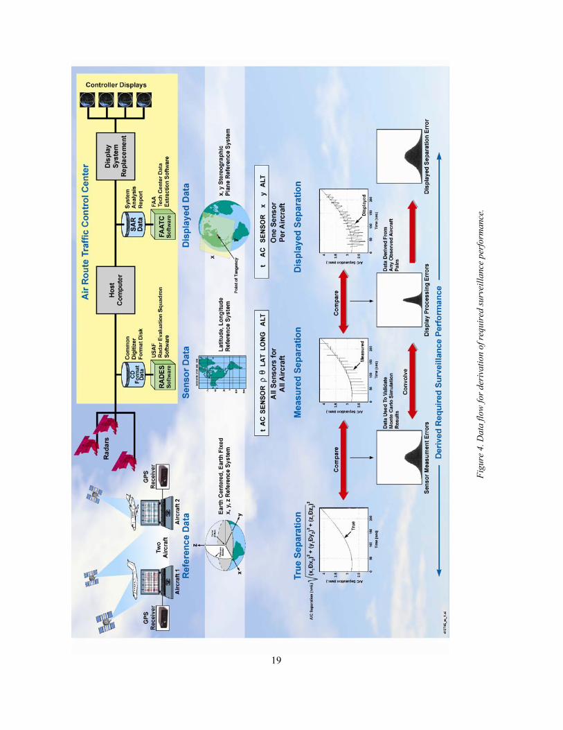
The RSP system in widespread use for 5-mile separation was chosen to be the long-range ATCRBS sliding window beacon sensor at a range of 200 nautical miles separating aircraft with a ground speed of 600 knots. These systems are normally operated in a mosaic environment. At the sort box boundaries between radar coverage areas there is normally “stitching” and “hopping” of targets as they cross from a sort box that has one radar assigned as primary sensor to another sort box which has a different assigned radar. For the purposes of this analysis it is assumed that using two different radars to track aircraft being separated as they cross sort box boundary lines is conditionally acceptable at sort box boundaries but not acceptable for the entire airspace. The RSP system in wide use is assumed to be the case where a single long-range sliding window sensor is tracking both aircraft. An MSSR long-range system is assumed for the new technology case. These cases are also summarized in Table 1.

For both the 3-mile separation case and the 5-mile separation case the aircraft were configured in-trail because this causes the most error in relative separation with asynchronous updates of the targets.

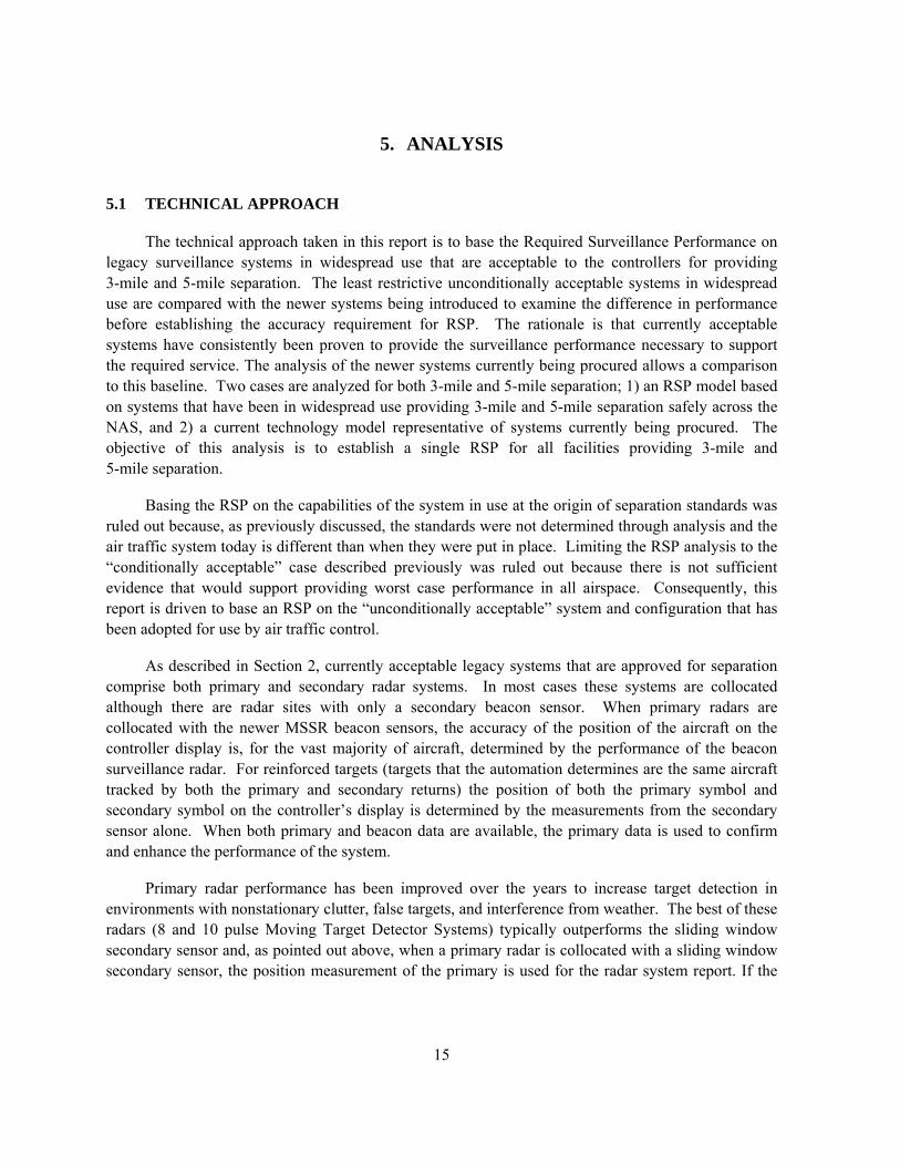
The error characteristics of primary and secondary radar systems and the RSP metric chosen are described below. This is followed by a description of the Monte Carlo analysis for the 3-mile separation and 5-mile separation to derive the sensor error contribution to RSP. The display system processing errors are measured by comparing data recorded in Common Digitizer format as it is received by the facility to the data recorded on the System Analysis Report (SAR) tapes; this approach is summarized in Figure 4 and further described in Section 5.7.

The sensor measurement errors are derived from the Monte Carlo analysis and verified by a flight test. The display system processing errors are measured from targets compared during normal operations. The errors in displayed separation are computed by sampling from both these distributions and also validated by flight tests. Individual flight tests alone cannot provide sufficient data to derive RSP with any statistical significance. The Monte Carlo analysis uses one million runs to produce the error distributions and the display processing errors are derived from many pairs of targets in diverse geometries over a long period of time. The flight test, which is described in detail in Section 6, serves to validate these computed errors. A program was developed that simulated the placement and performance of the radars recording data during the flight test and incorporated the same error models as the Monte Carlo simulation. This serves as a test of the validation techniques as data provided by the simulation is the same format as provided by the sensors during the flight test and is generated by using the same error model as the simulation.

Figure 4 also serves to illustrate the different reference systems used. The GPS sensors on-board the aircraft record data in an Earth Centered Earth Fixed reference system. The data reported by the sensors is range and azimuth from the sensor converted to latitude and longitude. The data provided to the controller is the x,y position as projected onto a flat plane touching the earth at a point of tangency, known as the stereographic plane. An excellent treatment of the various coordinate systems and how to transfer between them is contained in Misra and Enge9.

19

Figu

re 4

. Dat

a flo

w fo

r der

ivat

ion

of re

quir

ed su

rvei

llanc

e pe

rfor

man

ce.

20

5.2 ERROR CHARACTERISTICS OF SECONDARY RADAR SENSORS

Secondary radar error characteristics include both errors in estimating range and estimating azimuth to the target.

Range errors are due primarily to errors in measuring the interval between the instant an interrogation is sent from the radar to the time a reply is received from the aircraft’s transponder. This includes errors in the accuracy with which the sensor can measure the time interval and variations in the allowed turn around time of the transponder. Range errors due to timing are relatively small (< 200 feet) and do not increase with range. Refraction effects are only significant at very long range and were not included in this analysis. Propagation anomalies, such as atmospheric ducting, were also not included in this analysis for the same reason. Errors introduced by aircraft not equipped to report altitude were also not considered because those aircraft either have their altitude confirmed by the pilot or are not receiving separation services.

Azimuth measurement errors are primarily due to errors in estimating the target position within the beam width of the transmitted pulse. Azimuth measurement errors depend on the technique used to estimate the target’s position within the beam width. There are two azimuth measurement techniques used by secondary radars described earlier in this report.

The “sliding window” technique (illustrated in Figure 5) requires detection of replies in the leading and trailing edges of the beam where the signal is weakest. The azimuth of the target is estimated as the center of the reply train. FAA Beacon Interrogator BI-4 and BI-5 sensors use the sliding window technique. This technique is prone to azimuth inaccuracies or even target splits resulting from missing beacon replies. Interference from other interrogators or transponders can garble signals and cause missing replies. The performance also depends on whether the aircraft has a single transponder antenna on the bottom of the aircraft or two antennas, one on the top and one on the bottom of the aircraft. An aircraft with a single bottom mounted antenna may miss interrogations or have its reply blocked during a turn when the bottom of the aircraft is pointed away from the sensor.

Newer Monopulse Secondary Surveillance Radar (MSSR) sensors use multiple beam patterns for interrogations that allow an azimuth measurement from a single transponder reply. This technique (also illustrated in Figure 5) offers an approximately threefold improvement in azimuth measurement accuracy over the sliding window technique. FAA Mode S and BI-6 sensors use this monopulse technique for measuring azimuth. A detailed description of these two azimuth estimation techniques is given by Orlando.10 Figure 5 was taken from that article. A detailed description of secondary surveillance systems can be found in Stevens.11

21

Figure 5. Comparison of sliding window and monopulse azimuth measurement techniques.

Additional errors include residual registration errors caused by location and azimuth biases not removed by algorithms designed to align multiple sensors.

The position estimates are disseminated using the FAA Common Digitizer 2 (CD2) format. In this analysis the format resolution was not modeled as an additional error source but the position estimates were rounded to the allowed CD2 formats.

The scan time of the antenna determines the length of time between target updates. While the position estimates are not affected, the motion of the targets between their respective updates results in errors in displayed separation.

The radar source errors used in the analysis are presented in Table 2. The values of the errors used are based on radar specifications and field data from ARCON12 for radars in the Southern California TRACON, and from MIT Lincoln Laboratory13 for radars in the northeast region.

The errors for individual radars are in good agreement with the errors for radars reported in a study conducted by Lockheed Martin and included as an Appendix in the ARCON report.

Boresight

Antenna Antenna

“Sliding Window” Beacon Interrogator Monopulse Secondary Surveillance Radar

AircraftAzimuth

Measurement AircraftAzimuth

Measurement

ATCRBSReplies

Trailing-Edge Detection

Leading-Edge Detection

Boresight

Antenna Antenna

“Sliding Window” Beacon Interrogator Monopulse Secondary Surveillance Radar

AircraftAzimuth

Measurement AircraftAzimuth

Measurement

ATCRBSReplies

Trailing-Edge Detection

Leading-Edge Detection

22

Table 2 Error Sources Used in Monte Carlo Simulations for Beacon Sensors

Sensor Error Sources

1Note: MSSR handles both Mode S and ATCRBS transponders in a monopulse fashion. 2Note: For independent sensors tracking each aircraft. Same sensor scan time errors are deterministic. 3Note: ACP=Azimuth Change Pulse (1/4096 of a scan)

Transponder Error Sources

Mode S ATCRBS

Range Error ± 125 ft. (0.021 NM.) Uniform

σ = 72 ft. (0.012 NM.)

± 250 ft. (0.041 NM.) Uniform

σ = 144 ft. (0.024 NM.)

MSSR1 ATCRBS Sliding Window Short Range Long Range Short Range Long Range

Location Bias

200 ft. (0.033 NM.) Uniform in any direction σ = 115 ft. (0.019 NM.)

Registration

Errors Azimuth Bias

± 0.3º Uniform σ = 0.173º

Radar Bias

± 30 ft. (0.005 NM.) Uniform σ = 17 ft. (0.003 NM.)

Range Errors

Radar Jitter

25 feet rms Gaussian σ = 25 ft. (0.004 NM.)

Azimuth Error

Azimuth Jitter

Gaussian σ = 0.068º (0.8 ACP)3

Gaussian σ = 0.230º (2.6 ACP)3

Range 1/64 NM. Uniform σ = 27 ft.

(0.005 NM.)

1/8 NM. Uniform σ = 110 ft.

(0.018 NM.)


(0.005 NM.)


(0.018 NM.)

Data Dissemination Quantization CD format

Azimuth 360º/4096 Uniform σ = 0.025º

Uncorrelated Sensor Scan Time Error2

4–5 sec. Uniform σ = 219 ft.

(0.036 NM.)


(0.088 NM.)


(0.036 NM.)


(0.088 NM.)

23

5.3 REPORTING AND ERROR CHARACTERISTICS OF SURVEILLANCE SYSTEMS THAT INCLUDE PRIMARY RADARS

At most terminal and en route facilities there is a primary radar co-located with the beacon sensor. Both sensors independently make position estimates of targets and when the software determines that those position estimates are for the same aircraft the target reports are declared a “merged target” and the position report is characterized as “reinforced” meaning the beacon report and primary measurement reinforce each other. In the event a target is not reinforced it may be “beacon-only” meaning the primary did not report a target in a near enough position to reinforce the beacon report, or it may be characterized as “search-only” meaning the primary reported target was not reinforced with a beacon report. The position estimate is reported as range (rho) and angle (theta) from the sensor location. Beacon-only and search-only reports contain the rho, theta measurement of the respective sensor. For merged targets the position estimate of only one of the sensors is reported. Section 5.3.1 discusses the position measurements errors for primary radar. Section 5.3.2 discusses which sensor’s measurement is used for the position report in the event of a merged target.

5.3.1 Position Measurement Errors for Primary Radar

Modern primary radars employ narrowband Doppler filtering and distributed processing to improve target detection and position accuracy and lower false alarm rates. In good weather and with the absence of clutter the performance of modern radars in measuring position is better than a sliding window beacon sensor although not as good as a monopulse beacon sensor. The position measurement errors used for modeling the primary radar performance in this analysis are those specified for the Airport Surveillance Radar (ASR-9) primary radar14 in terminal mode and are presented in Table 3.

In the presence of weather, ground clutter, and airborne clutter the performance of a primary radar will degrade; in the worst cases it will not be able to see a target that is being tracked by the co-located beacon sensor. For that reason, and because there exist sliding window beacon-only sensors, the sliding window beacon performance is considered the baseline for acceptable performance when co-located with a primary radar. The model for assessing the primary radar performance need only consider conditions where its performance exceeds that of the beacon sensor.

24

Table 3 Sensor Error Sources Used in Monte Carlo Simulations for Primary Sensors

Location Bias 200 feet uniform in any direction

Registration Errors

Azimuth Bias

± 0.3° uniform

Radar Bias

± 30 feet uniform Range Errors

Radar Jitter

Gaussian σ = 275 feet

Azimuth Errors Azimuth Jitter Gaussian σ = 0.16° 1.8 ACP

Range

1/64 nautical mile Data Dissemination Quantization CD Format Azimuth

(360°/4096) = 1 ACP = 0.088°

Rotation Time

Motion of one aircraft relative to the other because of the

differences in measurement time is deterministic and depends on

the range and geometry

4–5 seconds

5.3.2 Source of Position Reports

Both primary and secondary radars measure the position of the target as rho (distance) and theta (angle). The format of the target reports currently provided is the Common Digitized 2 (CD2) format15,16 (found in Table 2) although other formats may be used in the future. Increased resolution of reporting format is often referenced as a way of increasing accuracy although the result of this analysis show that the errors are in general much larger than the CD2 resolution so increasing resolution will not necessarily increase accuracy. The CD2 format reports only one rho, theta measurement for merged targets. In the case of a sliding window sensor co-located with a primary radar, reinforced reports contain the rho, theta measurement of the primary radar although this is a site adaptable parameter and at least in the case of en route sensors this is sometimes adapted to report the beacon measurement. In the case of MSSR sensors, reinforced reports contain the rho, theta measurement of the beacon sensor. An MSSR sensor can be automatically (dual data processing channel failures) or manually placed in an Interim Beacon Interrogator (IBI) mode in which case it performs like a sliding window sensor and the primary position report will be used for reinforced targets.

25

5.4 ERRORS IN MEASURED SEPARATION FROM INDEPENDENT SURVEILLANCE SYSTEMS

The error in measured separation between two aircraft will depend on whether the positions of the two targets are reported by the same or independent surveillance sensors. Two factors add to the errors in the measured separation error displayed to a controller when independent sensors are reporting the aircraft positions; uncorrelated position measurement errors and differences in track update.

Surveillance systems will generally have bias errors associated with their position estimates. When the same sensor is used to measure the position of both targets, bias errors in position estimates associated with that sensor are not reflected in the separation measurement.

When a controller is separating two aircraft using the estimated positions on a display, the targets are updated at different times. This introduces an error in the displayed separation because of the motion of one aircraft relative to the other between updates. With a single sensor, for two target aircraft relatively near each other, the time between updates can be explicitly computed and is generally small. However, in the case of independent systems, the target updates are asynchronous and the time difference between target updates is generally larger, depending on the update rates of the independent sensors. This in turn can result in increased errors in displayed separation.

5.5 REQUIRED SURVEILLANCE PERFORMANCE ACCURACY METRIC

The Required Surveillance Performance accuracy metric refers to the standard of measurement performance that must be met to support the separation services provided by Air Traffic Control. One obvious possibility for the surveillance accuracy metric is the accuracy of the sensor in making target position measurements. There are two problems with using position accuracy as the primary metric for RSP. One is that Air Traffic Control provides a separation service rather than a positioning service. The other is that, as pointed out in Section 5.4, errors in measured separation depend on whether the same or independent sensors are providing the position estimates. The use of independent sensors with the same position measurement errors will result in relatively larger errors in measured separation. If the RSP is based solely on position measurement accuracy and set to allow the use of independent sensors, then currently acceptable single sensor performance would not meet the standard.

The approach taken in this analysis is to quantify the RSP in terms of limits on errors in measuring target separation displayed to the controller. This allows a direct comparison between single-sensor surveillance, and cases involving independent sensors or surveillance systems.

Additionally, there is no reason to assume that surveillance system position measurement errors will be Gaussian. Currently accepted sensors that provide 3-mile separation have non-Gaussian error contributors. If position measurement error is used as the RSP accuracy metric and it is assumed Gaussian then incorrect conclusions regarding the separation errors will likely be made.

26

For these reasons the RSP for accuracy derived in this analysis includes errors in displayed separation and expresses the requirement in terms of limits on the errors of the probability distribution of separation errors displayed to a controller.

Because controllers provide radar vectors to fixes and airports and are responsible for obstacle avoidance, the RSP includes a geographical accuracy requirement along with other attributes of legacy systems in defining the RSP. The other attributes included in the RSP are briefly discussed in Section 7.1 and are referenced from specifications; however the legacy systems define positional accuracy in terms that are not generally applicable to other technologies such as azimuth jitter. The sensor errors in Table 2 used to model the separation errors were used to generate the required geographic accuracy attribute in the RSP.

5.6 MONTE CARLO ANALYSIS OF SENSOR ERRORS

5.6.1 Monte Carlo Model Description

A Monte Carlo model was used in this analysis to quantify the distribution of errors in measured separation for the beacon sensors described above. A total of four cases were analyzed representing the errors in measured separation for the RSP model and the newest technology model for both the 3-mile separation and 5-mile separation cases, as described in Table 1. All of the characteristic radar errors were independently re-sampled for each trial using the errors in Table 2. One million trials were run to generate the error distributions described below. Separation measurement errors are highly dependent on range and relative geometry of aircraft and the radars. The analysis used randomly oriented two in-trail aircraft relative to the sensor for each trial.

The surveillance errors were sampled according to the error distributions described in Table 2 to produce estimated positions for each aircraft. These estimated positions were then reported in the CD2 format at the resolutions described in Table 2. Bias errors in the sensors were kept constant for sensor measurements of both targets. Reports for each aircraft were then used to compute estimated separation distances. The time between target updates was computed explicitly. The additional error caused by movement of the aircraft between updates was added to compute the separation error measured by the sensor(s).

The mean and standard deviation for the distributions were computed and reported. The error distributions generated by the simulations are not Gaussian because some of the source errors are uniform distributions. The kurtosis of a distribution is a measure of the “fatness” of the tails of distributions. A Gaussian distribution has a kurtosis of 3.0. The single sensor error distributions generated by the simulation had kurtosis measures of 3.8 to 4.4 indicating they are more prone to outliers than the Gaussian distribution.

27

5.6.2 3-Mile Separation

The procedure followed for the 3-mile separation cases was to determine the distribution of errors in measured separation observed, on average, for two aircraft that were three nautical miles apart in-trail as illustrated in Figure 6. Aircraft speed was chosen to be 250 knots (speed limit in the terminal area) as listed in Table 1. The aircraft were randomly oriented relative to the radar by randomly choosing an angle ϕ as illustrated in Figure 6 for each trial. The Monte Carlo simulations using the beacon error characteristics described in Table 2 were run for each of the cases listed in Table 1. The error characteristics of a primary radar as described in Table 3 were used to model the primary radar. Both the sliding window beacon sensor and the collocated primary radar cases are presented for the RSP case in Table 1 although, as described above, the sliding window beacon performance is considered the baseline acceptable performance. For both the 3-mile separation case and the 5-mile separation case the aircraft were configured in-trail because this causes the most error in relative separation with asynchronous updates of the targets.

Figure 6. Geometry for sensor error modeling for 3-NM separation.

Single Beacon Sensor Tracking Both Aircraft

Range to midpoint

ϕ

3 nmi in trail

Single Beacon Sensor Tracking Both Aircraft

Range to midpoint

ϕ

3 nmi in trail

28

The results of the one million trials for the cases listed in Table 1 are presented in Figures 7, 8, and 9 which show the distributions of sensor measured separation for aircraft that are actually 3 miles apart. The “jaggedness” in the distributions is due to the discrete allowed position reports of the CD2 format and the even distribution of the bin sizes in the histogram. There are a finite number of “allowed” separations and regardless of the size of the bins, more or less of the allowed reports will fall into one bin or another. If the number of trials is doubled, the graphs will look the same. If the histogram bin size is changed then a different “raggedness” pattern would appear.

Figure 7. Sensor separation estimate errors for a single ATCRBS sliding window short-range radar at a range of 40 miles and aircraft velocities of 250 knots.

1.5 2 2.5 3 3.5 4 4.50

1

2

3

4

5

6

7

8x 10

4

Estimated Separation (nautical miles)

Num

ber

of S

ampl

es (1

0000

00 T

otal

Tri

als)

Separation Estimates for a Single ATCRBS "Sliding Window" Short Range RadarRange 40 nautical miles, Aircraft Velocities 250 knots

μ = 3.0042 n. mi.σ = 0.1632 n. mi.

Actual Separation = 3.0 n. mi.

29

Figure 8. Sensor separation estimate errors for a single primary short-range radar at a range of 40 miles and aircraft velocities of 250 knots with little or no rain or clutter.

1.5 2 2.5 3 3.5 4 4.50

1

2

3

4

5

6

7

8x 104


Num

ber

of S

ampl

es (1

0000

00 T

otal

Tria

ls)

Separation Estimates for a Single ASR-9 Primary Short Range RadarRange 40 nautical miles, Aircraft Velocities 250 knots

μ = 3.0024 n. mi.σ = 0.1217 n. mi.


30

Figure 9. Sensor separation estimate errors for a single MSSR short-range radar at a range of 60 miles and aircraft velocities of 250 knots.

1.5 2 2.5 3 3.5 4 4.50

1

2

3

4

5

6

7

8x 104


Num

ber

of S

ampl

es (1

0000

00 T

otal

Tria

ls)

Separation Estimates for a Single MSSR Short Range RadarRange 60 nautical miles, Aircraft Velocities 250 knots

μ = 3.0012 n. mi.σ = 0.0799 n. mi.


31

The distributions of the error in measured separation for beacon and primary radar surveillance systems for the 3-mile separation cases described in Table 1 and shown in Figures 7–9 are presented in Table 4. The standard deviation of the distribution is given and the error limits within which 90%, 99%, and 99.9% of the distribution is contained are presented.

Table 4 Sensor Measured Separation Error Distribution Characterization for

Beacon and Primary Sensors for 3-NM Separation

3 NM Separation RSP Model Newest Technology Model

Sliding Window Short-Range

Sensor at 40-mile Range and Aircraft Velocities

of 250 knots

Terminal Primary Radar

Separating Aircraft

3 miles at Velocities of

250 knots with Little or No

Rain or Clutter

MSSR Short-Range

Sensor at 60-mile Range and Aircraft Velocities

of 250 knots

Standard Deviation of Separation Error

σ = 0.16 NM σ = 0.12 NM σ = 0.08 NM

Percentage of Error Distribution within

Limits

Error Limits

90% Within ± 0.28 NM Within ± 0.20 NM

Within ± 0.13 NM


Within ± 0.23 NM

99.9% Within ± 0.65 NM Within ± 0.46 NM

Within ± 0.32 NM

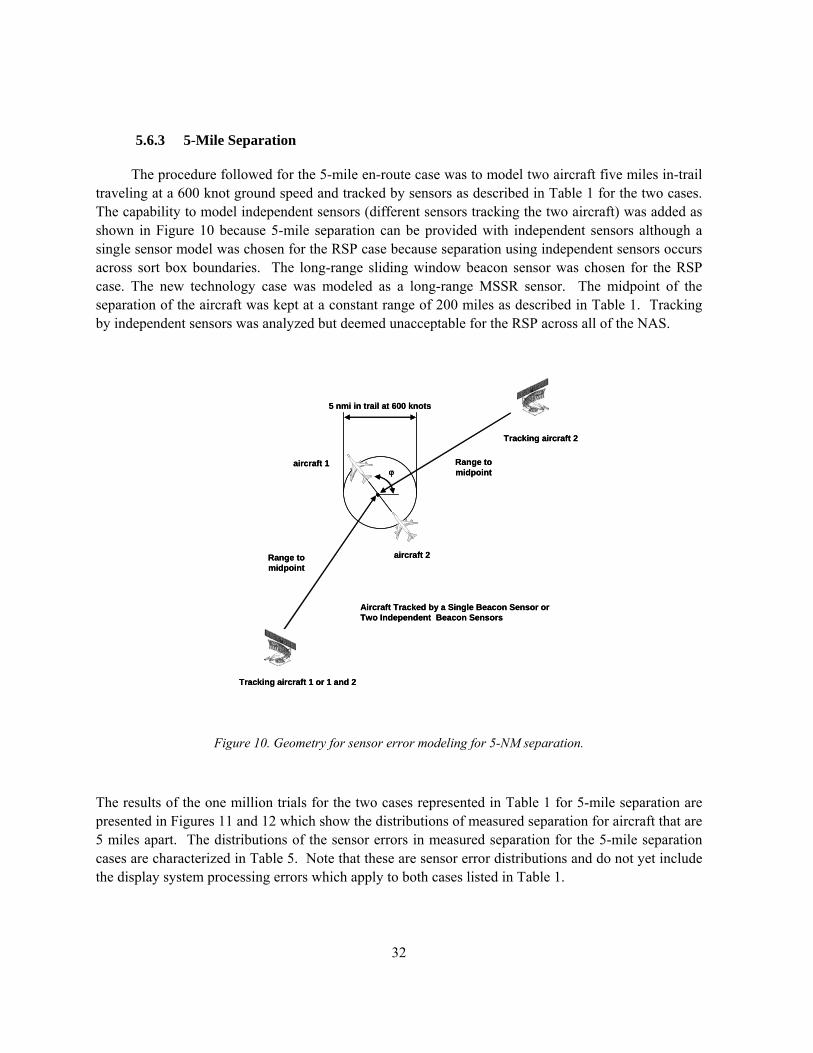
32

5.6.3 5-Mile Separation

The procedure followed for the 5-mile en-route case was to model two aircraft five miles in-trail traveling at a 600 knot ground speed and tracked by sensors as described in Table 1 for the two cases. The capability to model independent sensors (different sensors tracking the two aircraft) was added as shown in Figure 10 because 5-mile separation can be provided with independent sensors although a single sensor model was chosen for the RSP case because separation using independent sensors occurs across sort box boundaries. The long-range sliding window beacon sensor was chosen for the RSP case. The new technology case was modeled as a long-range MSSR sensor. The midpoint of the separation of the aircraft was kept at a constant range of 200 miles as described in Table 1. Tracking by independent sensors was analyzed but deemed unacceptable for the RSP across all of the NAS.

Figure 10. Geometry for sensor error modeling for 5-NM separation.

The results of the one million trials for the two cases represented in Table 1 for 5-mile separation are presented in Figures 11 and 12 which show the distributions of measured separation for aircraft that are 5 miles apart. The distributions of the sensor errors in measured separation for the 5-mile separation cases are characterized in Table 5. Note that these are sensor error distributions and do not yet include the display system processing errors which apply to both cases listed in Table 1.

Aircraft Tracked by a Single Beacon Sensor or Two Independent Beacon Sensors

Range to midpoint

ϕ

5 nmi in trail at 600 knots

Range to midpoint

Tracking aircraft 1 or 1 and 2

Tracking aircraft 2

aircraft 1

aircraft 2

Aircraft Tracked by a Single Beacon Sensor or Two Independent Beacon Sensors

Range to midpoint

ϕ

5 nmi in trail at 600 knots

Range to midpoint

Tracking aircraft 1 or 1 and 2

Tracking aircraft 2

aircraft 1

aircraft 2

33

Figure 11. Separation estimate errors for single sensor long-range ATCRBS sliding window sensor at a range of 200 miles and aircraft velocities of 600 knots.

0 1 2 3 4 5 6 7 8 9 100

0.5

1

1.5

2

2.5

3

3.5

4x 104


Num

ber o

f Sam

ples

(100

0000

Tot

al T

rials

)

Separation Estimates for a Single ATCRBS "Sliding Window" Long Range RadarRange 200 nautical miles, Aircraft Velocities 600 knots

μ = 5.0669 n. mi.σ = 0.8025 n. mi.


34

Figure 12. Separation estimate errors for single sensor long-range MSSR sensor at a range of 200 miles and aircraft velocities of 600 knots.

0 1 2 3 4 5 6 7 8 9 100

0.5

1

1.5

2

2.5

3

3.5

4

4.5

5x 104


Num

ber o

f Sam

ples

(100

0000

Tot

al T

rials

)

Separation Estimates for a Single MSSR Long Range RadarRange 200 nautical miles, Aircraft Velocities 600 knots

μ = 5.0084 n. mi.σ = 0.2566 n. mi.


35

Table 5 Sensor Measured Separation Error Distribution Characterization for

Beacon Sensor Errors for 5-NM Separation

5.7 DISPLAY SYSTEM PROCESSING ERRORS

The two cases listed in Table 1 for 5-mile separation contain “HOST processing” under the display system processing caption. Display system processing refers to the automation system that receives the sensor position reports at a facility and translates those reports into a display on the controller’s screen. The 3-mile separation cases in Table 1 labeled “direct to glass” assume that a single sensor directly feeds the display.

Display system processing errors are introduced by the system between the sensor reports and the separation displayed to the controller on the screen. The differences between separation as measured by sensor reports and separation displayed to the controller may result from display latencies, coordinate transformation, asynchronous updates, and missed updates or tracking errors. The

5-NM Separation RSP Model Newest Technology Model

Single Sliding Window Long-Range Sensor at 200-mile Range and Aircraft Velocities of

600 knots

Single MSSR Long-Range Sensor at 200-mile Range and Aircraft Velocities of

600 knots

Standard Deviation of Separation Error

σ = 0.80 NM σ = 0.25 NM

Percentage of Error Distribution within

Limits

Error Limits




36

display system processing errors depend on the system design and automation software, as well as whether the aircraft are being tracked by the same radar or different radars. The HOST system in the Air Route Traffic Control Centers (ARTCCs) was chosen as representative because it is in such widespread use.

Display system processing errors were measured from data rather than modeled. This was accomplished by comparing the separation of targets based on sensor reports received at the Boston Air Route Traffic Control Center to the separation of the same targets on the controller’s display. As shown in Figure 4 in Section 5.1, the CD2 data reported by the sensors is recorded as USAF RADar Evaluation Squadron (RADES) format data as it enters the facility. The position reports are recorded in latitude and longitude based on the rho, theta reports of the individual sensors. All reports of sensors tracking targets are recorded; consequently there will be multiple reports for each aircraft being tracked. The separation displayed to the controller is computed from the position reports as recorded on the System Analysis Report (SAR) tapes. The position reports include the beacon code, time, and the Cartesian (x,y) position on the stereographic plane. Each ARTCC displays target positions on a stereographic plane as illustrated in Figure 4 with a point of origin (x=0, y=0) and point of tangency (where it touches the earth) defined for that facility’s airspace. All target position reports received from field sensors are projected onto that common plane. The position report from only one sensor is provided to the controller’s display for a given target and that is the position report recorded in a file on the SAR tape. The SAR data, in a separate file, records which sensor is being utilized for reports for a given target as a function of time. Thus it is possible to determine which sensor’s target data were presented to the controller and the x,y position on the stereographic plane that was used to present the target position. The time between the SAR recording and the display is assumed negligible.

In order to compare the separation reported by the sensors to that displayed to the controllers, both recorded RADES data and SAR data tapes for a period of 1045–1415 UTC on October 6, 2005 were obtained from the Boston Air Route Traffic Control Center. The RADES data files were sent to MIT/Lincoln Laboratory and the copied SAR data tapes sent to the FAA’s William J. Hughes Technical Center (WJHTC) in Atlantic City, New Jersey.

The RADES data files were examined at MIT/Lincoln Laboratory and 50 aircraft pairs were manually selected, using as a criteria that the aircraft pair were in close horizontal proximity over an extended period of time (tens of minutes) and were at the same or nearly the same altitudes. An example of the flight paths of the two aircraft in one of the cases selected is shown in Figure 13. The fifty cases were identified to WJHTC by providing the two beacon codes, the start and stop times, and the approximate latitude and longitude. WJHTC then processed the SAR tapes based on the case descriptions and provided MIT/Lincoln Laboratory with the SAR data of the beacon codes of interest, which included two files for each case. One file contained the sensor used as a function of time for each of the two beacon codes and the other contained the time, beacon code, x,y position on the stereographic plane, and Mode C reported altitude for each report.

37

Figure 13. Sample tracks of two aircraft from the RADES data being tracked by the Stewart radar at Boston ARTCC.

The RADES data files, which contain data for all radars, were filtered to create files that matched the sensors identified by the SAR data as those used for display on the controller’s screen. The separation as a function of time between the targets in the RADES data was computed by converting the latitude and longitude reports to the Earth Centered Earth Fixed (ECEF) reference grid and computing the separation at each update report. This separation was computed each time a beacon target produced a new position report. The separation of the beacon targets as reported in the SAR data was computed directly from the x,y position reports representing position on the stereographic plane, and was also updated with each beacon report.

38

The computed separation between the two beacon targets as a function of time as recorded by the sensors (RADES data) and as presented to the controller (SAR data) was compared. An example of a plot comparing the RADES and SAR data is shown in Figure 14.

Figure 14. Comparison of measured separation versus time from the RADES data and the SAR data for a sample case.

The difference between the two reported separations as a function of time was measured for each update to provide a histogram of the differences in separation for each case. This represents a probability distribution of the errors introduced by the display system processing between what was reported by the sensors and what was displayed to the controllers for a single case of two aircraft being separated for a period of time. The histogram for the example case shown in Figures 13 and 14 is shown in Figure 15. The non-zero mean shown in Figure 15 is typical of the cases analyzed since the geometry of the flight paths relative to the radar are not random for a given case.

4.93 4.935 4.94 4.945 4.95 4.955 4.96 4.965 4.97 4.975 4.98

x 104

10

12

14

16

18

20

22

Time in seconds

sepa

ratio

n in

nau

tical

mile

s

Separation in nautical miles for SAR data and rades data Radar 1: SWF Tracking Aircraft 1: 1535Radar 2: SWF Tracking Aircraft 2: 2616

SAR dataRADES data

39

Figure 15. Typical histogram of difference between sensor measurement of separation in the RADES data and displayed separation in the SAR data. Fifty cases were summed to measure display system processing error.

Of the 50 cases chosen only 39 were able to be reduced from the SAR data. This was in part due to multiple aircraft with the same beacon code in the SAR data and in part due to unavailable SAR tapes for the total time of interest. These 39 cases were added together and normalized to take out any bias introduced by the particular selection of cases. The display system processing errors are different depending on whether a single sensor is tracking both aircraft or different sensors are tracking the two aircraft. When multiple sensors track aircraft and there is a switch between the sensor providing the track there are typically gaps in coverage due to different radars sampling at different times. Occasionally this is exacerbated if the track switches back and forth between two sensors several times in succession. This is one of the main contributors to the tails of the independent sensor display system processing errors. There are far fewer “outliers” in the single sensor case and those are due to missed updates of one of the aircraft.

-2.5 -2 -1.5 -1 -0.5 0 0.5 1 1.5 20

5

10

15

Difference in separation for SAR and Rades data (nmi)

Num

ber o

f occ

uren

ces

Histogram of errors in displayed separationRadar 1: SWF tracking AC: 1531 and Radar 2: SWF tracking AC: 7122

40

Two display system processing error models probability distributions were developed, one for the single sensor model and one for the independent sensor model. The final results are the distributions of HOST display system processing errors presented in Figure 16 for single sensors and Figure 17 for independent sensors. In the final analysis only the single sensor display processing errors were used to establish the RSP as shown in Table 1.

Figure 16. Histogram of HOST display system processing errors for single sensor measured from 39 sample cases of aircraft pairs recorded at Boston ARTCC on October 6, 2004.

-4 -3 -2 -1 0 1 2 3 40

2

4

6

8

10

12x 104

Difference in Separation for SAR and RADES data (nautical miles)

Num

ber

of o

ccur

ence

s

Single Sensor Model: Errors in Displayed Separation

41

Figure 17. Histogram of HOST display system processing errors for multiple sensors measured from 39 sample cases of aircraft pairs recorded at Boston ARTCC on October 6, 2004.

5.8 TOTAL SYSTEM ERRORS TO THE DISPLAY

The 5-mile separation cases listed in Table 1 include HOST display system processing for a single sensor. The results of convolving the single sensor display sensor processing errors with the sensor errors for the 5-mile separation cases are presented in Figures 18 and 19.

The results of sampling from the single sensor display system processing errors shown in Figure 16 and the single sensor sliding window long-range radar errors shown in Figure 11 are presented in Figure 18 as the total system error for the 5-mile separation RSP case. Convolving the display system processing error distribution with the sensor distribution has a smoothing effect on the sensor error histogram lessening the effect of the discrete CD2 position reports.

-4 -3 -2 -1 0 1 2 3 40

2

4

6

8

10

12x 104

Difference in Separation for SAR and RADES data (nautical miles)

Num

ber o

f occ

uren

ces

Independent Sensors Model: Errors in Displayed Separation

42

Figure 18. Total system error for long-range sliding window sensor at 200 mile range with single sensor HOST system display processing.

0 1 2 3 4 5 6 7 8 9 100

0.2

0.4

0.6

0.8

1

1.2

1.4

1.6

1.8

2x 104


Num

ber

of S

ampl

es (1

0000

00 T

otal

Tri

als)

Separation Estimates for a Single ATCRBS "Sliding Window" Long Range RadarWith Display System Processing Errors for a Single Sensor Added

Range 200 nautical miles, Aircraft Velocity 600 knots

μ = 5.0669 n. mi.σ = 0.8107 n. mi.


43

The results of randomly sampling the single sensor display system processing errors shown in Figure 18 and the single sensor MSSR long-range radar errors shown in Figure 12 are presented in Figure 19 as the total system error for the 5-mile separation newest technology case.

Figure 19. Total system error for long-range MSSR system at 200 mile range and aircraft at 600 knots with HOST system display processing for a single sensor.

0 1 2 3 4 5 6 7 8 9 100

0.5

1

1.5

2

2.5

3

3.5

4x 104


Num

ber

of S

ampl

es (1

0000

00 T

otal

Tri

als)

Separation Estimates for a Single MSSR Long Range RadarWith Display System Processing Errors for a Single Sensor Added

Range 200 nautical miles, Aircraft Velocity 600 knots

μ = 5.0077 n. mi.σ = 0.2821 n. mi.


44

The results of convolving the display system processing errors for the 5-mile separation cases with the sensor errors provide the total system errors. Table 6 provides the distribution descriptions of total system error for the 5-mile separation cases.

Table 6 Total System Measured Separation Error Distribution

Characteristics for 5-NM Separation Cases

5-NM Separation RSP Model Newest Technology Model

Single Sliding Window Long-Range Sensor at 200-mile Range and Aircraft Velocities of 600 knots with Single Sensor HOST Display

System Processing Errors

Single MSSR Long-Range Sensor at 200-mile Range and Aircraft Velocities of 600 knots with Single Sensor HOST Display

System Processing Errors

Standard Deviation 0.81 NM 0.28 NM

Percentage of Error Distribution Within

Limits

Error Limits




45

6. FLIGHT TEST VALIDATION

6.1 PURPOSE

The purpose of the flight test was to validate the modeled error sources of the sensors used in the analysis by comparing true separation, as provided by position recordings from GPS on-board two aircraft, with sensor measured separation as recorded from sensors at Boston Air Route Traffic Control Center. This was accomplished by flying two aircraft approximately three miles apart in-trail over a large portion of Boston Center airspace. The flight path was designed to provide data from at least nine of the fourteen sensors in Boston Center airspace including long-range and short-range beacon sensors and sliding window and MSSR sensors. The use of two aircraft allowed a comparison of measured separation with true separation rather than measuring the accuracy of the position report of the aircraft. Measured separation error is the metric used in the analysis.

6.2 DATA RECORDING

6.2.1 Airborne Data Recording

The airborne data recording portion of the flight test validation recorded WGS-84 Earth Centered Earth Fixed (ECEF) reference position data from two GPS receivers, one in each aircraft. An Ashtech Model GG24 GPS plus Glonass sensor, shown in Figure 20, was used in both aircraft.

Figure 20. Ashtech Model GG24 GPS plus Glonass sensor.

46

The GG surveyor provides position accuracy on the order of 7–20 meters17 and updates position once per second. This position information was sent to a laptop via a serial port connection. GPSLog, a custom-written program, wrote the updated reports to a file on disk. GPSLog utilizes a 9600 baud 8N1 serial communication format to communicate with the GG Surveyor. The software uses a 1.0 second timer to poll the GPS for its current position, allowing for a more robust connection. If the GPS fails to reply to a poll in a timely fashion, the operator is notified and can begin troubleshooting. Additionally, the GG Surveyor has the capability of recording position updates to internal memory for later offline retrieval, providing a backup of the data recording.

The flight test validation made use of Lincoln Laboratory’s Falcon 20 and Gulfstream G2 jet aircraft. The Falcon 20 is shown below in Figure 21, and the G2 is shown in Figure 22. Each of the test aircraft carried a GPS/Laptop recording system and operator, and provided a GPS antenna.

Figure 21. Falcon 20 lead aircraft in flight test.

47

Figure 22. Gulfstream G2 trailing aircraft in flight test.

After completion of the flight test validation, the recorded GPS data were post-processed to obtain time-stamped ECEF position reports in a form that could be read into MATLAB. All analysis was done in MATLAB. GPS time does not incorporate the “leap seconds” used in Universal Time Coordinated (UTC) time and the current offset between GPS and UTC time is thirteen seconds. This difference was subtracted and the data analyzed was in UTC time.

48

6.2.2 Ground Data Recording

The ground data recording portion of the flight test validation consisted of two separate systems, as previously shown in Figure 4 of Section 5. The sensor data consisted of a recording of all the Common Digitizer 2 (CD2) format messages from the 14 radars in the USAF RADar Evaluation Squadron (RADES) format. Screenshots of representative data available from RADES are shown in Figures 23 and 24 below. Ten different sensors actually tracked the two test aircraft during the flight.

Figure 23. Typical RADES screenshot of flight paths of all aircraft being tracked by all sensors.

49

The data view screen lists a row for each report of each sensor color coded by message type, red for beacon only, green for search (primary only) and blue for reinforced. The sample data illustrated in Figure 24 was filtered to eliminate the search reports. The data can also be filtered by sensor(s) and beacon codes.

Figure 24. RADES data viewer sample screen.

50

The RADES software was used to extract, time, rho, theta, latitude, longitude, and altitude for both test aircraft from all sensors that tracked the two test aircraft. These data files were converted to a format that could be read into MATLAB.

The data displayed to the controller was recorded on System Analysis Report (SAR) tapes. These tapes are produced by software running on the host computer and record all of the display updates sent to the Display System Replacement (DSR) screen. These tapes were sent to the FAA’s William J. Hughes Technical Center (WJHTC) in Atlantic City, New Jersey for post-processing. The product of this processing was a file containing time, aircraft ID, radar ID, (x, y) position on the stereographic plane, and altitude for the test aircraft. The SAR data contains only the data from the sensor that was used to display the target on the controller’s screen. This file was then read into MATLAB for further processing and comparison of the displayed separation to the measured separation as well as the GPS truth data.

6.3 FLIGHT PATH

The flight path was coordinated with Boston Center to provide maximum exposure to various types of sensors. The aircraft were cleared as a flight-of-two from Bedford MA. to fly to WOONS intersection and then direct to Norwich VOR, Calverton VOR, Madison VOR, Hartford VOR, Chester VOR, BRATS intersection, Keene VOR, LOBBY intersection and return to Bedford at Flight Level 240. The path is illustrated below in Figures 25 and 26 of the flight test results.

6.4 FLIGHT TEST SIMULATION

A flight test simulation program was developed to model the beacon sensors and aircraft track geometries for the flight test in Boston Center airspace. All of the Boston Center sensors were located on the stereographic plane and the flight tracks of the two aircraft were input as straight lines between the waypoints. The x,y positions on the stereographic plane were used for all position measurements in the model. The sensor errors were modeled according to the errors in Table 2. Radar site location bias errors, range bias errors, azimuth bias errors, and registration errors were sampled once per radar and held constant. The aircraft transponder errors were also sampled once and held constant. The sensor antenna position at the start of the simulation and its rotation rate was sampled once for each sensor. The simulation computed if either of the target test aircraft was within range of a given sensor and when each of the sensors would hit each of the aircraft and then computed a measured position based on the bias errors and jitter errors. The bias errors were held constant for each sensor and the jitter errors were sampled for each hit. The simulation sensor measurements were then converted to CD2 format and recorded. The data created by the simulation is in the same format as the recorded RADES data which allows for a direct qualitative comparison.

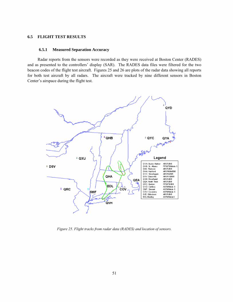
51

6.5 FLIGHT TEST RESULTS

6.5.1 Measured Separation Accuracy

Radar reports from the sensors were recorded as they were received at Boston Center (RADES) and as presented to the controllers’ display (SAR). The RADES data files were filtered for the two beacon codes of the flight test aircraft. Figures 25 and 26 are plots of the radar data showing all reports for both test aircraft by all radars. The aircraft were tracked by nine different sensors in Boston Center’s airspace during the flight test.

Figure 25. Flight tracks from radar data (RADES) and location of sensors.

52

Figure 26. Radar hits of flight test aircraft recorded by RADES during the flight test.

53

A qualitative comparison of the position reports of the RADES data and the flight test simulation described in Section 6.4 were made for selected straight line segments of the flight test. Sample plots comparing the RADES data recorded from the sensors and data generated by the simulation for the same geometry using the modeled errors are shown for a portion of the flight test in Figures 27–30. The recorded data from RADES shows less dispersion than the simulation results using the modeled errors indicating better performance from the sensors than expected.

Figure 27. Position data generated by the simulation over a portion of the flight test path for the Falcon.

-72.7 -72.68 -72.66 -72.64 -72.62 -72.6 -72.58 -72.5641

41.01

41.02

41.03

41.04

41.05

41.06

41.07

41.08

41.09

41.1

Longitude (degrees)

Latit

ude

(deg

rees

)

AC1 Falcon: Simulation Longitude-Latitude Position

GPS truth

QXU

QHA

QVH

QEA

QRC

PVD

QIE

BDL

54

Figure 28. Position data measured by RADES over a portion of the flight test path for the Falcon.

-72.7 -72.68 -72.66 -72.64 -72.62 -72.6 -72.58 -72.5641

41.01

41.02

41.03

41.04

41.05

41.06

41.07

41.08

41.09

41.1

Longitude (degrees)

Latit

ude

(deg

rees

)

AC1 Falcon: RADES and GPS Longitude-Latitude Position

GPS truth

QXU

QHA

QVH

QEA

QRC

PVD

QIE

BDL

55

Figure 29. Position data generated by the simulation over a portion of the flight test path for the Gulfstream.

-72.28 -72.26 -72.24 -72.22 -72.2 -72.18 -72.16 -72.14 -72.12 -72.1 -72.0841.34

41.36

41.38

41.4

41.42

41.44

41.46

41.48

Longitude (degrees)

Latit

ude

(deg

rees

)AC2 Gulfstream: Simulation Longitude-Latitude Position

GPS truth

QXU

QHA

QVH

QEA

QRC

PVD

QIE

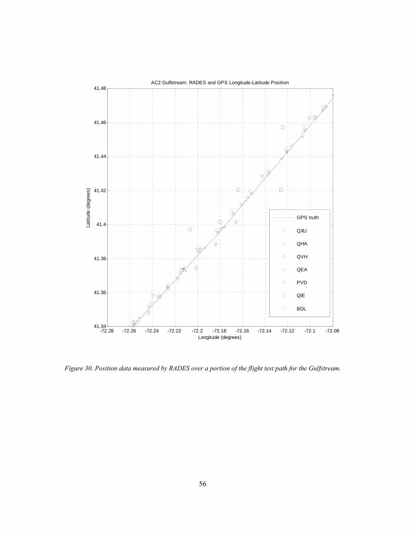
56

Figure 30. Position data measured by RADES over a portion of the flight test path for the Gulfstream.

-72.28 -72.26 -72.24 -72.22 -72.2 -72.18 -72.16 -72.14 -72.12 -72.1 -72.0841.34

41.36

41.38

41.4

41.42

41.44

41.46

41.48

Longitude (degrees)

Latit

ude

(deg

rees

)AC2 Gulfstream: RADES and GPS Longitude-Latitude Position

GPS truth

QXU

QHA

QVH

QEA

PVD

QIE

BDL

57

The GPS position data recorded on-board the flight test aircraft consisted of WGS-84 Earth Centered Earth Fixed (ECEF) x,y,z positions of the aircraft updated every second. Figure 31 is a plot of the position reports as recorded by the GPS units. Flight test aircraft safety procedures required that the data recording be off during take-off and landing as seen by gaps in the tracks at the beginning and end of the flight test. The GPS time was corrected to Coordinated Universal Time (UTC) time by subtracting 13 leap seconds from the recorded GPS time.

Figure 31. Flight tracks from GPS for Falcon and Gulfstream.

58

A comparison of the GPS data and RADES data indicated a clock bias had been introduced into the RADES data since the previous analysis for the display system processing described in Section 5.7. It appears that the RADES data were recorded on a computer that was not time synchronized with UTC. This was verified by converting the ECEF GPS position reports to latitude and longitude and comparing the position to that reported in the RADES data. An offset (subtraction) of 35 seconds from the RADES data centered latitude and longitude measurements from all sensors around the GPS data for both aircraft. A sample of the data is shown in Figures 32–35 which is the latitude data for the Gulfstream aircraft. Results were similar for longitude and latitude for both aircraft for all sensors indicating a time offset in the RADES recorded data. This time correction was applied to all analysis of the RADES data.

Figure 32. Gulfstream latitude measurements from GPS and time corrected RADES, all tracking sensors.

52500 53000 53500 54000 54500 55000 55500 56000 56500 5700040.5

41

41.5

42

42.5

43

43.5

Time (s)

Latit

ude

(deg

)

Gulfstream Latitude vs. Time- Corrected

GPSRADES

59

Figure 33. Gulfstream latitude measurements from GPS and time corrected RADES, all tracking sensors, enlargement of Turn 1.

53500 53550 53600 53650 53700 53750 53800 53850 53900

40.8

40.85

40.9

40.95

41

41.05

41.1

41.15

Time (s)

Latit

ude

(deg

)


GPSRADES

60


54700 54750 54800 54850 54900 54950 55000 55050 55100

42.75

42.8

42.85

42.9

42.95

43

43.05

43.1

Time (s)

Latit

ude

(deg

)


GPSRADES

61


55700 55750 55800 55850 55900 55950 56000 56050 56100

42.95

43

43.05

43.1

43.15

43.2

43.25

Time (s)

Latit

ude

(deg

)


GPSRADES

62

The GPS data were recorded as Earth Centered Earth Fixed (ECEF) (x,y,z) position measured in meters from the center of the earth. The GPS positions recorded during the flight test are shown in Figures 36 and 37.

Figure 36. Earth centered, Earth fixed GPS position of Falcon.

0 500 1000 1500 2000 2500 3000 3500 40001.35

1.4

1.45

1.5

1.55x 106

Time (s)

X P

os (m

)

Falcon ECEF X Position

0 500 1000 1500 2000 2500 3000 3500 4000-4.7

-4.6

-4.5

-4.4x 106

Time (s)

Y P

os (m

)

Falcon ECEF Z Position

0 500 1000 1500 2000 2500 3000 3500 40004.1

4.2

4.3

4.4x 10

6

Time (s)

Z P

os (m

)

Falcon ECEF Z Position

63

Figure 37. Earth centered, Earth fixed GPS position data for Gulfstream.

The GPS position data were used to compute the 3-dimensional separation of the aircraft. Because the two GPS units were independent, the outputs were not synchronized so the data were interpolated to common times. The 3-dimensional separation was converted to horizontal separation using the Mode C reported altitudes of the aircraft interpolated to these same times. Computations showed that the 100-foot resolution in the Mode C altitude reports contribute insignificant errors. The GPS separation was considered “truth” in the remainder of the analysis and used to measure the errors in the RADES and SAR data in separation measurement. The aircraft separation during the flight test is shown in Figures 38 and 39.

0 500 1000 1500 2000 2500 3000 3500 40001.35

1.4

1.45

1.5

1.55x 106

Time (s)

X P

os (m

)G2 ECEF X Position

0 500 1000 1500 2000 2500 3000 3500 4000-4.7

-4.6

-4.5

-4.4x 106

Time (s)

Y P

os (m

)

G2 ECEF Y Position

0 500 1000 1500 2000 2500 3000 3500 40004.15

4.2

4.25

4.3

4.35x 106 G2 ECEF Z Position

Time (s)

Z P

os (m

)

64

Figure 38. Separation between the Falcon and Gulfstream during the flight versus time (GPS data).

0 500 1000 1500 2000 2500 3000 3500 40000

5

10

15

20

25

Time (s)

Hor

izon

tal S

epar

atio

n (n

m)

Separation vs. Time

Testbegins

Testends

Takeoff

Flyout

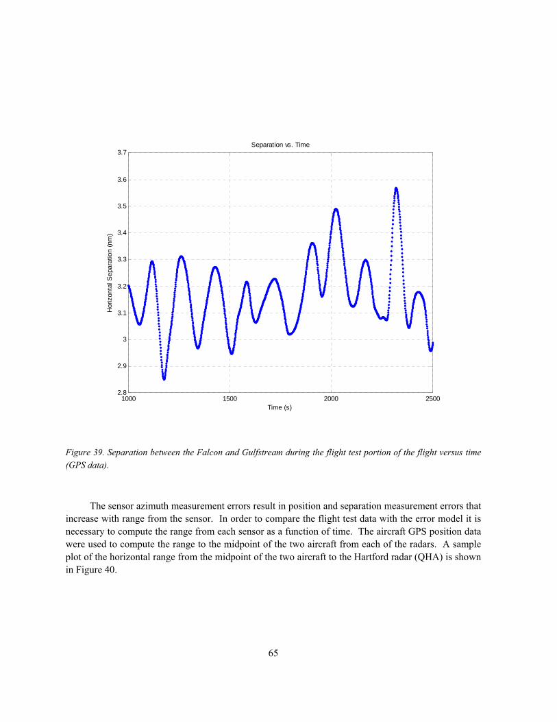
65

Figure 39. Separation between the Falcon and Gulfstream during the flight test portion of the flight versus time (GPS data).

The sensor azimuth measurement errors result in position and separation measurement errors that increase with range from the sensor. In order to compare the flight test data with the error model it is necessary to compute the range from each sensor as a function of time. The aircraft GPS position data were used to compute the range to the midpoint of the two aircraft from each of the radars. A sample plot of the horizontal range from the midpoint of the two aircraft to the Hartford radar (QHA) is shown in Figure 40.

1000 1500 2000 25002.8

2.9

3

3.1

3.2

3.3

3.4

3.5

3.6

3.7Separation vs. Time

Time (s)

Hor

izon

tal S

epar

atio

n (n

m)

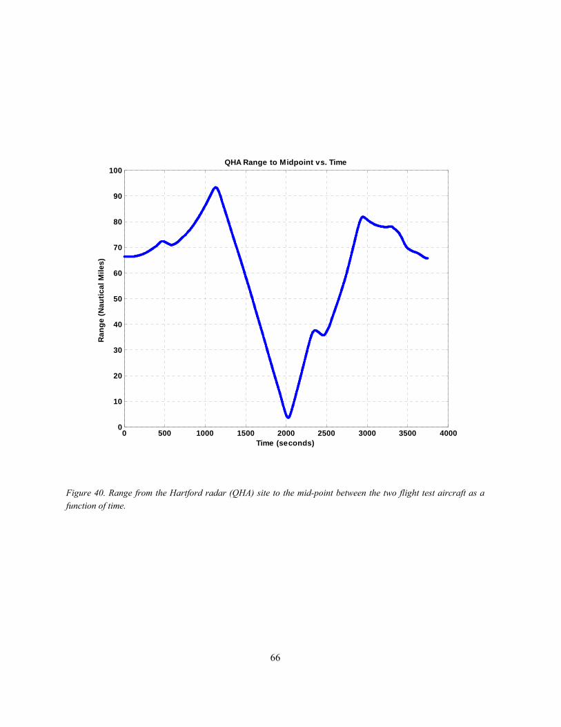
66

Figure 40. Range from the Hartford radar (QHA) site to the mid-point between the two flight test aircraft as a function of time.

0 500 1000 1500 2000 2500 3000 3500 40000

10

20

30

40

50

60

70

80

90

100

Time (seconds)

Ran

ge (N

autic

al M

iles)

QHA Range to Midpoint vs. Time

67

The RADES data were examined to determine periods of time during the flight test when each sensor was tracking both aircraft with continuous updates. This was done by plotting the delta update times for both aircraft as a function of time and noting periods where there were no points above the normal update rate. An example plot of the delta times between updates as a function of time for both aircraft is shown in Figure 41 for the Hartford radar (QHA). The two arrows denote time periods when the sensor was tracking both aircraft without interruption.

Figure 41. Example of update delta times versus time for the Hartford radar (QHA) tracking both flight test aircraft.

52000 52500 53000 53500 54000 54500 55000 55500 56000 56500 5700010

20

30

40

50

60

70

80

Time (s)

Δ U

pdat

es (s

)

QHA Updates vs. Time

FalconG2

68

The position measurements for both aircraft for the periods of continuous coverage were then determined for each sensor. Figure 42 illustrates the track of the two aircraft as measured by the Hartford radar (QHA) during the time period shown in the example above.

Figure 42. Position reports of the flight test aircraft during continuous tracking of both aircraft by the Hartford radar (QHA).

The position measurement of the two flight test aircraft were used to compute the separation measurement of the sensor as a function of time. The sensor reported ρ, θ, and the aircraft reported Mode C altitude were converted to a local Cartesian coordinate system and the horizontal separation was computed for the aircraft as a function of time. Although the actual separation of the aircraft is a continuous function of time the measured separation will be a discrete function with each change in the value indicative of a radar report update of one of the aircraft. Continuing with the Hartford radar (QHA) example, the plot of separation as a function of time for the two time periods of continuous tracking is shown in Figure 43.

-73 -72.5 -72 -71.5 -71

41

41.2

41.4

41.6

41.8

42

42.2

42.4

42.6

42.8

43

Longitude (deg)

Latit

ude

(deg

)

Radar Measured Position- QHA

FalconG2

69

Figure 43. Separation of the flight test aircraft as a function of time as measured by the Hartford radar (QHA).

The two aircraft separated by three miles are updated within a short time period. An algorithm was developed to determine the separation measurement a short time after the second aircraft update. Continuing with the Harford radar (QHA) example, the red lines in Figure 44 illustrate examples of the times sampled to compare the measured separation with the true separation. Each point in time represented by the red line indicates a single data point for measured separation by the sensor.

54200 54400 54600 54800 55000 55200 55400 556000

1

2

3

4

5

6

Time (s)

Sep

arat

ion

(nm

)

52800 53000 53200 53400 53600 53800 540000

1

2

3

4

5

Time (s)

Sep

arat

ion

(nm

)

Radar Measured Separation vs. Time- QHA

70

Figure 44. Sampled measurements of the separation of the aircraft by the Hartford radar (QHA).

These separation measurements, for each radar, were then compared to the GPS separation which is considered true and the difference is recorded as a measured separation error. These errors are then plotted as individual data points as a function of range. The range is taken from the range versus time plots computed earlier for each particular sensor. This procedure is used for all radars and is combined on plots designed to show the modeled sensor error limits as shown in Figures 45–47 for MSSR and sliding window sensors. The lines on the figures drawn as a function of range and shown in the legend represent the lines where the model predicts 1% and 10% of the errors to fall below and above respectively. Thus 1% of the measured errors would be expected to exceed the upper solid line and 1% of the errors predicted to fall below the lower solid line. The lines are not perfectly symmetric about zero because by convention the absolute value of the negative measured separation error can never exceed the actual separation. The numbers on the figures represent the number of flight test data points measured in that error region and the number predicted by the model based on the total number of data points. Thus in Figure 45 1% of the 496 data points or approximately 5 data points would be expected to exceed the upper solid line and 10% or approximately 50 to exceed the upper dotted line. Thus 45

53400 53420 53440 53460 53480 53500 53520 53540 53560 53580 536001

1.5

2

2.5

3

3.5

4

4.5

5

Time (s)

Sep

arat

ion

(nm

)Radar Measured Separation vs. Time- QHA

55000 55020 55040 55060 55080 55100 55120 55140 55160 55180 552001.5

2

2.5

3

3.5

4

4.5

Sep

arat

ion

(nm

)

Time (s)

71

points would be predicted to fall between the upper dotted and solid lines. It was a coincidence that exactly 496 data points were recorded for both the MSSR and sliding window sensors. Note the expanded scale for the sliding window sensor in Figure 46 compared to the MSSR plot shown in Figure 45. Figure 47 is a re-plot of the MSSR sensors shown in Figure 46 but with the same scale of the sliding window plot shown in Figure 46.

Figure 45. Modeled error limits versus range for MSSR sensors.

0 20 40 60 80 100 120 140 160 180 200-1

-0.8

-0.6

-0.4

-0.2

0

0.2

0.4

0.6

0.8

1MSSR Single Sensor

Range from sensor to midpoint of two aircraft (nmi.)

Mea

sure

d se

para

tion

erro

r pe

rcen

tile

limits

(nm

i.)

4

38

428

23

3

Flight Test Data Points in Region

Total Number of Data Points: 496

(Predicted by Model)

(5)

(5)

(45)

(45)

(396)

1% predicted below and above10% predicted below and aboveQHBQHAQRCPVDBDL

72

Figure 46. Modeled error limits versus range for sliding window sensors.

0 20 40 60 80 100 120 140 160 180 200-3

-2

-1

0

1

2

3Sliding Window Single Sensor


Mea

sure

d se

para

tion

erro

r pe

rcen

tile

limits

(nm

i.)

2

12

474

7

1

Flight Test Data Points in Region

Total Number of Data Points: 496

Both Aircraft Reinforced1 Aircraft Beacon OnlyBoth Aircraft Beacon Only

(Predicted by Model)

(5)

(5)

(45)

(45)

(396)

1% predicted below and above10% predicted below and aboveQIEQXUQVHQEA

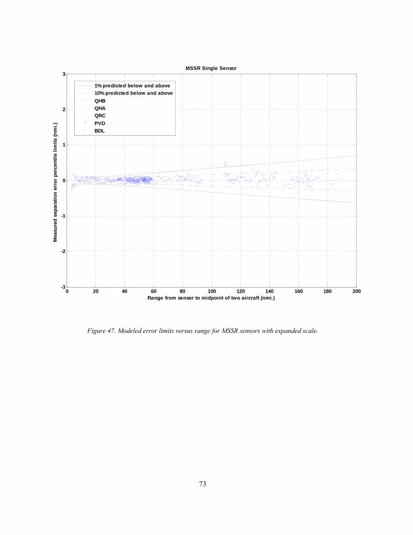
73

Figure 47. Modeled error limits versus range for MSSR sensors with expanded scale.

0 20 40 60 80 100 120 140 160 180 200-3

-2

-1

0

1

2

3MSSR Single Sensor


Mea

sure

d se

para

tion

erro

r per

cent

ile li

mits

(nm

i.)

1% predicted below and above10% predicted below and aboveQHBQHAQRCPVDBDL

74

There is not enough data available from a one hour flight to be statistically definitive, especially because the performance of the sensors is a function of range to the various sensors being recorded which was continually changing. Still, some conclusions regarding the sensor measurement performance can be seen from Figures 45–47. There seems to be good agreement between the model and the separation measurements made by MSSR sensors as shown in Figure 46. The performance of the sliding window beacon sensors seems to be somewhat better than predicted by the model as shown in Figure 47, at least in the number of points falling outside the 1%, 10%, 90% and 99% regions. The outliers were investigated and it was found that in all cases the measurements were made as track was being lost by a sensor and there was a lapse in the update of one or both of the aircraft, which was not considered in the model. The better than expected performance of the sliding window sensors warranted further investigation, especially because of the good agreement for the MSSR sensors. Since the only difference in the modeled error between the MSSR sensors and the sliding window sensors was the azimuth jitter distribution, a study of the azimuth jitter performance is presented in Section 6.5.2 below.

6.5.2 Sensor Azimuth Performance

The performance of the sliding window sensors as measured during the flight test was better than predicted by the error model while the measured MSSR performance was more closely predicted by the model. As the only difference in the model of the MSSR and sliding window sensors was the modeled azimuth jitter errors, a more detailed investigation of the azimuth (θ) errors of the sliding window and MSSR sensors was undertaken.

The RADES data contained the azimuth (θRADES) measurement for all sensors for both aircraft which is based on the antenna position relative to true north. The GPS data contained the aircraft position in Earth Centered Earth Fixed (ECEF) coordinates which was converted to latitude and longitude. Since the location of the sensors was known in latitude and longitude the bearings from the sensors (θGPS) could be computed using spherical trigonometry. The total errors in azimuth were defined as θRADES – θGPS where the GPS measurements were interpolated such that there was a GPS value for each RADES measurement.

The total azimuth errors for both aircraft as a function of time were plotted. A curve fit using the lowest power polynomial that removed any bias from the residuals was used to determine the bias in the measurement. Azimuth bias in a sensor can be a slowly varying function of time or a function of the relative bearing from the sensor. The measurement of two test aircraft in trail made it possible to determine that a sensor bias was affecting both aircraft. The residuals about the curve fitted bias were computed as the azimuth jitter. These measurements were used to generate a probability distribution of bias and jitter for each sensor.

75

This process is illustrated in Figures 48–50 for Remson (QXU), a long-range sliding window sensor, and Figures 51–53 for Bradley (BDL), an MSSR sensor. The improved azimuth jitter performance of the MSSR sensor is evident in these examples.

Figure 48. Theta error measurements on both flight test aircraft as a function of time for the Remson radar (QXU), a long-range sliding window sensor.

0 500 1000 1500 2000 2500 3000 3500-1

-0.8

-0.6

-0.4

-0.2

0

0.2

0.4

0.6

0.8

1

time (seconds)

azim

uth

erro

r (de

gree

s)

QXU (ARSR-4 BI5)Azimuth error (RADES-GPS)

4617 G24665 Falcon

76

Figure 49. Curve fitting of the Remson (QXU) theta error data.

0 500 1000 1500 2000 2500 3000 3500-1

-0.5

0

0.5

1

time (seconds)

azim

uth

jitte

r (d

egre

es)

residuals

0 500 1000 1500 2000 2500 3000 3500-1

-0.5

0

0.5

1

time (seconds)

tota

l azi

mut

h er

ror

(deg

rees

)

QXU (ARSR-4 BI5)Total azimuth error (RADES-GPS)

y = - 3.3e-015*x4 + 1e-011*x3 + 5e-008*x2 - 0.00014*x + 0.073

data bias fit

77

Figure 50. Separation of the azimuth error (θ) into azimuth bias and jitter for the Remson (QXU) long-range sliding window sensor.

-0.3 -0.2 -0.1 0 0.1 0.2 0.30

20

40

60

80

100

QXU (ARSR-4 BI5)Bias Error

μ = 0.026

σ = 0.039

-1 -0.8 -0.6 -0.4 -0.2 0 0.2 0.4 0.6 0.8 10

5

10

15

20

QXU (ARSR-4 BI5)Jitter Error

μ = 5.3e-017

σ = 0.122

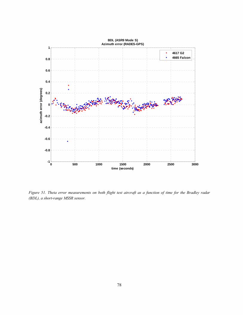
78

Figure 51. Theta error measurements on both flight test aircraft as a function of time for the Bradley radar (BDL), a short-range MSSR sensor.

0 500 1000 1500 2000 2500 3000-1

-0.8

-0.6

-0.4

-0.2

0

0.2

0.4

0.6

0.8

1

time (seconds)

azim

uth

erro

r (de

gree

s)BDL (ASR9 Mode S)

Azimuth error (RADES-GPS)

4617 G24665 Falcon

79

Figure 52. Curve fitting of the Bradley (BDL) theta error data.

500 1000 1500 2000 2500-1

-0.5

0

0.5

1

time (seconds)

azim

uth

jitte

r (de

gree

s)

residuals

0 500 1000 1500 2000 2500 3000-1

-0.5

0

0.5

1

time (seconds)

tota

l azi

mut

h er

ror (

degr

ees)

BDL (ASR9 Mode S)Total azimuth error (RADES-GPS)

y = 2.3e-022*x7 - 2.3e-018*x6 + 8.8e-015*x5 - 1.7e-011*x4 + 1.6e-008*x3 - 6.5e-006*x2 + 0.00061*x + 0.043

data bias fit

80

Figure 53. Separation of the azimuth error (θ) into azimuth bias and jitter for the Bradley (BDL) short-range MSSR sensor.

In two cases the data for a sensor was divided into parts because of discontinuities caused when the aircraft passed close to the sensor. An example is shown in Figure 54 for the Hartford (QHA) sensor. The other case was the data from the Riverhead (QVH) sensor which was divided into three parts.

-0.3 -0.2 -0.1 0 0.1 0.2 0.30

10

20

30

40

50

60

BDL (ASR9 Mode S)Bias Error

μ = 0.003

σ = 0.054

-1 -0.8 -0.6 -0.4 -0.2 0 0.2 0.4 0.6 0.8 10

20

40

60

80

BDL (ASR9 Mode S)Jitter Error

μ = 2.4e-014

σ = 0.050

81

Figure 54. Theta error measurements on both flight test aircraft as a function of time for the Hartford radar (QHA), an MSSR sensor exhibiting a discontinuity in the bias as the aircraft passed near the sensor.

The procedure described above was done for all nine sensors. The standard deviation (σ) of the theta (θ) jitter error of each sensor is plotted in Figure 55 and compared to the modeled error for the monopulse (MSSR) and sliding window sensor. Four of the five MSSR sensors performed slightly better than the error model and one slightly worse. Because the performance of QHB was close to three of the sliding window sensors it is not possible to rule out that the sensor may have been in IBI mode and acting as a sliding window sensor. Three of the four sliding window sensors performed much better than the error model and one performed very close to the model. This indicates that there is a relatively wider spectrum of performance in the sliding window sensor.

0 500 1000 1500 2000 2500 3000 3500 4000-1

-0.8

-0.6

-0.4

-0.2

0

0.2

0.4

0.6

0.8

1

time (seconds)

azim

uth

erro

r (de

gree

s)

QHA (FPS-67B BI6)Azimuth error (RADES-GPS)

4617 G24665 Falcon

82

Figure 55. Standard deviation (σ) of azimuth jitter errors for the nine sensors recording both flight test aircraft; errors for sliding window sensors compared to MSSR sensors.

All of the measured jitter errors were combined for the five MSSR and four sliding window sensors and the probability distributions for the respective jitter errors computed. These are shown in Figure 56 for the MSSR sensor and in Figure 57 for the sliding window sensors.

QEA QIE QVH QXU QHA QHB QRC BDL PVD0

0.05

0.1

0.15

0.2

0.25

σ de

gree

s

Standard Deviation (σ) of Azimuth Jitter Errors

Modeled error for sliding window sensors

Modeled error for MSSR sensors

← may be in IBI mode

monopulsesliding window

83

Figure 56. Distribution of azimuth jitter errors for all MSSR sensors.

-1.5 -1 -0.5 0 0.5 1 1.50

50

100

150

200

250

300

350

400

450

500

Azimuth jitter (degrees)

Azimuth Jitter for all MSSR Sensors

σ = 0.058 degrees

84

Figure 57. Distribution of azimuth jitter errors for all sliding window sensors.

-1.5 -1 -0.5 0 0.5 1 1.50

50

100

150

200

250

300

σ = 0.15 degrees

Azimuth jitter (degrees)

Azimuth jitter for all Sliding Window sensors

85

The cumulative average theta jitter standard deviation for the MSSR sensors was σ = 0.058 degrees which is in very good agreement with the modeled error source of σ = 0.068 degrees. The measurements from five sensors is not statistically significant enough to change the error model keeping in mind that the error model is for the least performing system, not the average performance of all systems.

The cumulative average theta jitter standard deviation for the sliding window sensors was σ = 0.15 degrees which is less than the error model source of σ = 0.23 degrees. However, one sliding window sensor performed very close to the error model indicating a range of performance in sliding window sensors. The error model is designed to model the least performing system of its design and so when there is a relatively wide range of performance, the average performance will be statistically better than the lesser performing sensors. The ARCON12 report notes a similar result in their field measurements of ARSR sliding window beacon sensors in Southern California Tracon with a σ = 0.119 degrees at a range of greater than 60 miles although they list a typical error of σ = 0.23 degrees.

The difference in the way the sliding window and MSSR sensors work provides an explanation of why the sliding window performance will have a larger range in performance than the MSSR sensors. Newer MSSR sensors use multiple beam patterns for interrogations that allow an azimuth measurement from a single transponder reply. MSSR sensors with selective interrogation provide excellent surveillance in heavy traffic environments with high interrogation rates from multiple sensors. Sliding window sensors will perform very well when replies are received across the beam width, typically 15 to 20 hits per beam. However, in dense traffic or a dense interrogator environment, the performance of a sliding window sensor deteriorates. Interrogation efficiency decreases when many interrogators are active. This includes other ground based sliding window or MSSR sensors as well as airborne interrogations from Traffic Alert and Collision Avoidance System (TCAS). The aircraft transponder may be suppressed or actively replying to another interrogation and not reply to a given interrogation from a sensor. In addition the reply may be garbled if it overlaps with the reply from another transponder. This can cause relatively large errors (on the order of a tenth of a beam width or 0.25 degrees) in azimuth measurements if the missed replies are near the edge of the beam. The data from the flight test was taken in a low interrogation environment at a time and altitude where there was not heavy traffic and so the higher performance is consistent with the performance of sliding window sensors in a benign environment. The error model must account for the performance in more challenging environments.

The bias data from all of the sensors was combined to provide a probability distribution of the bias errors, and is presented in Figure 58. The error model assumed a uniform bias error of plus or minus 0.3 degrees which has a σ = 0.173 degrees. The data from the flight test shown in Figure 58 has a σ = 0.15 degrees which is in good agreement but the distribution does not appear to be uniform. This will only affect cases using independent sensor where bias errors are not correlated and in the final analysis there were no cases using independent sensors to establish an RSP. The sensor theta bias error model will be modified for future analysis.

86

Figure 58. Distribution of azimuth bias errors for all sensors.

-1.5 -1 -0.5 0 0.5 1 1.50

100

200

300

400

500

600

700

800

900

1000

σ = 0.15 degrees

Azimuth bias (degrees)

Azimuth bias for all sensors

87

6.5.3 Measurement of Radar Report Latencies

The flight test data position measurements were used to analyze the radar report latencies. The RADES data represents the time the data entered the facility and the SAR data represents the total latency from sensor measurement to display to the controller.

As previously mentioned in Section 6.5.1 there was a 35-second average time offset between the GPS data and RADES data. This was due to a clock bias that was not observed in previous data recordings, i.e., those used in the Display Processing Errors in Section 5.7. As shown in Figure 59 below, time offsets for multiple sensors consist of both the clock bias common to all sensors and sensor specific latencies. Clock bias is the difference in time between two clocks and latency is the difference between the time for which a measurement is made and the time it is delivered.

Figure 59. Diagram showing the relationship between clock bias, latency, and time offset.

The sensor latency cannot be computed without first determining the clock bias, if it exists. However, because the clock bias is the same for all sensors, the difference in time offset between the sensors is a measure of the variance in latencies.

The three data sources (GPS, RADES, and SAR) each had its own time stamp which allowed time offsets throughout the system to be analyzed. The SAR data time stamp based on a UTC

88

measurement at the facility appears accurate; however, it is not possible to verify this from measurements of the time difference in GPS data and SAR data. The offsets were computed for both RADES and SAR data, using the GPS time stamps as reference data. The time offset for the radar reports was determined by examining data from each radar individually and minimizing the difference in position reports between the radar (RADES or SAR) data and the GPS data.

The time offset for each sensor was determined by finding the offset (Δt) that minimized the difference in position measurements between the sensor and GPS data for all measurements.

For the RADES data, the time offsets were calculated by minimizing differences in reported latitude and longitude as illustrated in a sample plot shown in Figure 60. The figure provides an illustration of how adding the optimal time offset best aligns the RADES data with the GPS data for the QEA radar. Using these time offsets allows the errors in measured separation to be calculated independently of any timing errors.

Figure 60. Example of RADES versus GPS data used to compute time offset.

53300 53400 53500 53600 53700 53800 53900 5400040.8

40.9

41

41.1

41.2

41.3

41.4

Time (s)

Latit

ude

(deg

)

QEA Offset= -35 sec

Original RecordingRecording w/ OffsetGPS Position

89

The SAR data errors were calculated using ECEF x,y,z position reports. For the SAR data, the mathematical approach was to determine the Δt that minimized the sum of the differences in x, y, and z:

min iii i zyx Δ+Δ+Δ∑

Figure 61 illustrates a time offset computation for the SAR data, while Figure 62 is a blown-up illustration showing the relationship between Δ t and Δ xi . The Δ t was varied until the sum of all Δ xi , Δ yi , and Δ zi for both aircraft was minimized.

Figure 61. Example of SAR versus GPS data used to calculate absolute latency.

5.544 5.546 5.548 5.55 5.552 5.554 5.556 5.558 5.56

x 104

1.516

1.517

1.518

1.519

1.52

1.521

1.522

1.523

x 106 GPS vs. SAR data time offset of 1.1 seconds

Time in seconds (s)

X p

ositi

on in

met

ers

(m)

Original Recordingrecording with offsetGPS Position

90

Figure 62. Illustration showing the relationship between Δt and Δx.

Nine radars tracked the test aircraft and the corresponding RADES data were used to calculate time offsets, with an average offset of 35.5 seconds. Of those nine radars, four were reported in the SAR data and the average time offset was calculated to be 1.7 seconds. Timing discrepancies between RADES and GPS data are most likely due to an incorrect clock setting in the RADES recording system, while the timing differences between SAR and GPS data could be due to processing latency. See Table 8 for individual results. Only radars that tracked the test aircraft in the RADES or SAR reports are displayed.

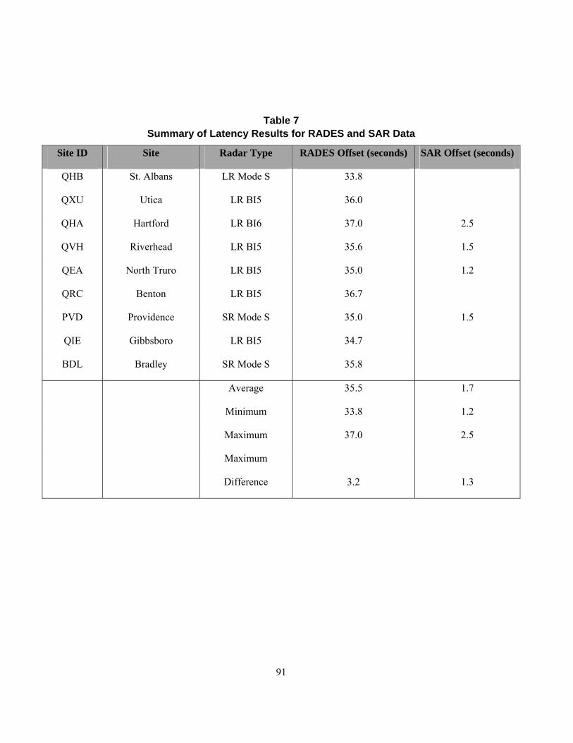
91

Table 7 Summary of Latency Results for RADES and SAR Data

Site ID Site Radar Type RADES Offset (seconds) SAR Offset (seconds)

QHB St. Albans LR Mode S 33.8

QXU Utica LR BI5 36.0

QHA Hartford LR BI6 37.0 2.5

QVH Riverhead LR BI5 35.6 1.5

QEA North Truro LR BI5 35.0 1.2

QRC Benton LR BI5 36.7

PVD Providence SR Mode S 35.0 1.5

QIE Gibbsboro LR BI5 34.7

BDL Bradley SR Mode S 35.8

Average 35.5 1.7

Minimum 33.8 1.2

Maximum 37.0 2.5

Maximum

Difference 3.2 1.3

92

93

7. STATEMENT OF REQUIRED SURVEILLANCE PERFORMANCE

7.1 SELECTION OF RSP

Required Surveillance Performance consists of many attributes. The focus of this analysis was on surveillance accuracy required to support 3-mile and 5-mile separation. The accuracy requirements were derived from Monte Carlo simulations of modeled legacy sensor errors and validated with flight test data. Accuracy in measured separation was the metric chosen as described in Section 5.5, however geographical position accuracy is also available from the simulation and included as an additional attribute.

The RSP accuracy requirement was derived from the cases listed in Table 1 for 3-mile and 5-mile separation. The sensor in the 3-mile separation case is the short-range primary collocated with a sliding window beacon sensor at a range of 40 miles tracking two aircraft 3-miles in trail at 250 knots. The baseline error in measured separation is taken to be that of the beacon sensor. Though the primary sensor is slightly more accurate it can degrade in clutter environments and in those cases it is the beacon sensor that is used to provide separation. Also, MSSR sensors can be used to provide 3-mile separation when they go into the IBI mode and their performance is that of a sliding window sensor. The sensor is in a single site adaptation, i.e., the same sensor is providing position information for both aircraft. No display system processing errors were included; it was assumed the reports went “direct to glass” as is the nominal case for TRACONS.

The 5-mile separation case is for a single long-range sliding window sensor at a range of 200 miles tracking aircraft five miles in trail at 600 knots. The total error in separation was determined by independently sampling from the sensor error distribution and the experimentally measured HOST display sensor processing error distribution and adding these errors. This is the nominal system in use at ARTCCs today.

The flight test data validated the accuracy, and provided update rate, and latency values. The remainder of the RSP attribute values use the reference system approach based on the specifications of representative sensors as noted in the respective tables. It is not clear that new systems must meet all of the other attributes of current legacy systems but if not, some safety analysis is required.

The following tables summarize the RSP separation accuracy requirements and other attributes of a surveillance system necessary for 3-mile and 5-mile separation and the performance achieved by currently acceptable systems. New systems that meet or exceed all RSP attributes will provide surveillance performance necessary to support 3-mile and 5-mile separation. It may be that candidate surveillance systems can trade off performance between some of the attributes but that would require further analysis on a case by case basis.

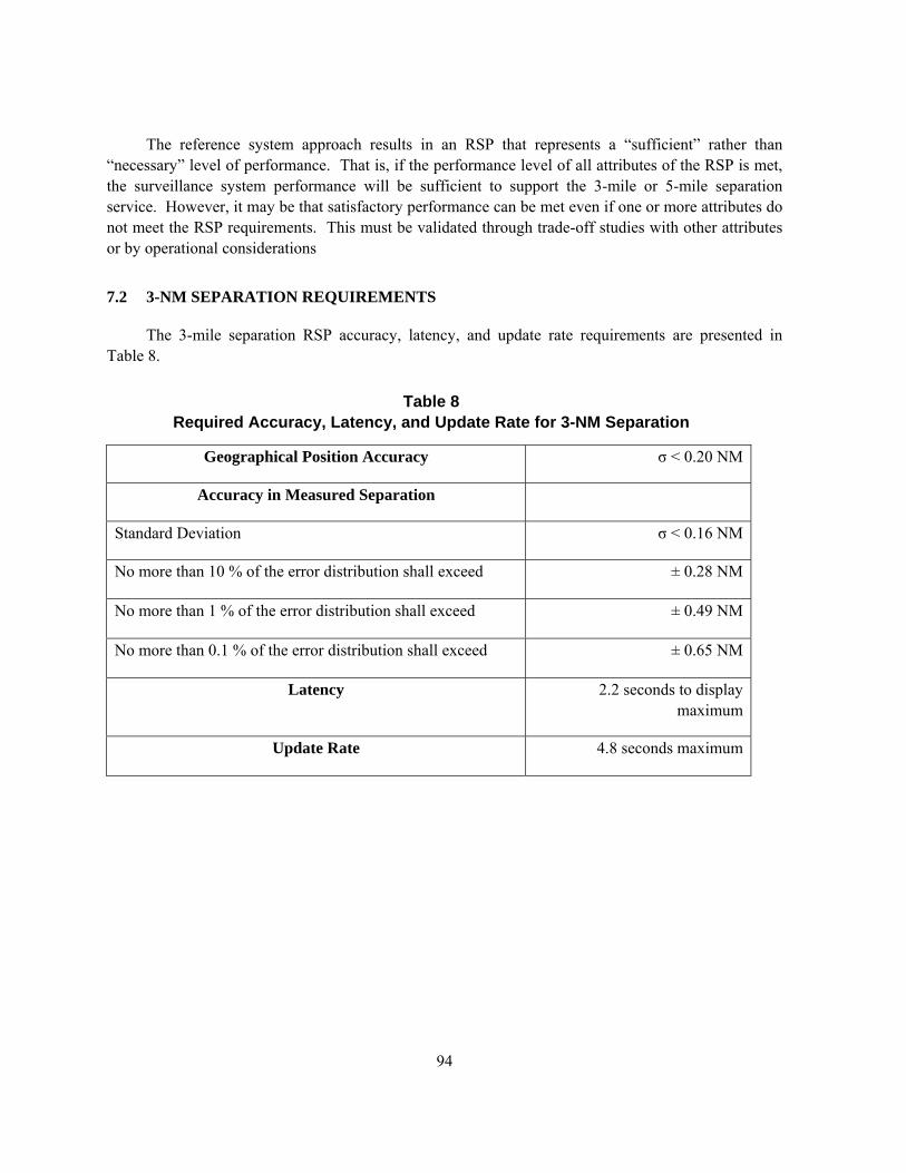
94

The reference system approach results in an RSP that represents a “sufficient” rather than “necessary” level of performance. That is, if the performance level of all attributes of the RSP is met, the surveillance system performance will be sufficient to support the 3-mile or 5-mile separation service. However, it may be that satisfactory performance can be met even if one or more attributes do not meet the RSP requirements. This must be validated through trade-off studies with other attributes or by operational considerations

7.2 3-NM SEPARATION REQUIREMENTS

The 3-mile separation RSP accuracy, latency, and update rate requirements are presented in Table 8.

Table 8 Required Accuracy, Latency, and Update Rate for 3-NM Separation








Update Rate 4.8 seconds maximum

95

7.3 5-NM SEPARATION REQUIREMENTS

The 5-mile separation RSP accuracy, latency, and update rate are presented in Table 9.

Table 9 Required Accuracy, Latency, and Update Rate for 5-NM Separation








Update Rate 12 seconds maximum

96

97

8. SUMMARY AND CONCLUSIONS

Historically, requirements for the performance of new surveillance systems have been based on the assumption that these systems performed in a similar manner to the existing rotating secondary and primary radar systems. This is not the case for new systems being proposed and a fundamental change in concept for the method of approving such systems is needed. Consequently, international standardization is increasingly based on Required Total System Performance (RTSP) specifications that are independent of the particular technology or implementation that is used to support a service. The term Required Surveillance Performance (RSP) is the subset of RTSP that is concerned with the surveillance requirements needed to support various services. This report is concerned with the RSP to support 3-mile and 5-mile separation services.

The approach taken in this report to establishing requirements to provide 3-mile and 5-mile separation is the reference system approach; one of two approaches recognized by the International Civil Aviation Organization (ICAO). In the reference system approach the requirements for providing a service are based on a reference system that has proven to safely and satisfactorily support that service. The other approach, Target Level of Safety, is based on analysis that attempts to prove the absolute safety of an alternate technology and prove that it fits within an allowed safety budget. This is a more involved approach and is considered more appropriate for new services. A reference system approach has the advantage of a proven safety record. The approach taken in this analysis was to examine the error characteristics of the various types of surveillance sensors in the FAA inventory and to analyze their performance with regard to providing accurate separation measurements to controllers.

The separation measurement accuracy, latency, and update rate have been established for the Required Separation Performance to support 3-mile and 5-mile separation in the NAS based on existing legacy radar sensors regularly utilized in the National Airspace System. The modeled performance was validated through a flight test of two aircraft flying three-miles in trail in Boston ARTCC airspace and recording true position with on-board GPS units. Sensor data from all sensors reporting the position of the aircraft to the Boston facility was recorded as well as the recording of data used to generate the display on the controller’s scope. Flight test data on targets of opportunity was also used to measure the errors introduced through HOST display system processing.

These RSP attributes are applicable to the extent a surveillance system is similar in performance characteristics to the legacy systems used to derive a baseline. It is important to note that the reference system approach results in an RSP that represents a “sufficient” rather than “necessary” level of performance. That is, if the performance level of all attributes of the RSP is met, the surveillance system performance will be sufficient to support the 3-mile or 5-mile separation service. However, it may be that satisfactory performance can be met even if one or more attributes do not meet the RSP requirements. This must be validated through trade-off studies with other attributes or by operational considerations.

99

LIST OF ACRONYMS

ADS-B Automatic Dependent Surveillance Broadcast ARSR Air Route Surveillance Radar ARTCC Air Route Traffic Control Center ASR Airport Surveillance Radar ATCRBS Air Traffic Control Radar Beacon System BDL Designation for the Bradley CN ASR9/Mode S radar BI Beacon Interrogator CD2 Common Digitizer 2 (data format) DSR Display System Replacement ECEF Earth Centered Earth Fixed reference system FAA Federal Aviation Administration GPS Global Positioning System HF High Frequency HOST NAS automation host computer IBI Interim Beacon Interrogator ICAO International Civil Aviation Organization Mode A,C Modes for ATCRBS transponders, A simple, C including altitude reports,

(Mode B was never implemented) Mode S Mode Select Beacon System MSSR Monopulse Secondary Surveillance Radar NAS National Airspace System NM Nautical Mile PVD Designator for the Providence RI ASR9/Mode S radar QEA Designator for the North Truro MA ARSR/BI5 radar QHA Designator for the Hartford CN radar QHB Designator for the St. Albans VT FPS67B/Mode S QIE Designator for the Gibbsboro NJ ARSR/BI5 radar QRC Designator for the Benton, PN FPS67B/BI5 QVH Designation for the Riverhead NY ARSR/BI6 radar QXU Designation for the Remson NY ARSR/BI6 radar RADES USAF RADar Evaluation Squadron

100

RNP Required Navigation Performance RSP Required Surveillance Performance RTSP Required Total System Performance SAR System Analysis Report SCRSP Surveillance and Conflict Resolution Systems Panel TCAS Traffic Alert and Collision Avoidance System TLS Target Level of Safety TRACON Terminal Radar Approach Control facility UHF Ultra High Frequency UTC Universal Time Coordinated VHF Very High Frequency VOR Very High Frequency (VHF) Omni-directional Range WJHTC FAA’s William J. Hughes Technical Center in Atlantic City, New Jersey

101

REFERENCES

[1] ICAO, “Global Air Navigation Plan for CNS/ATM Systems Second Edition–2002,” Doc 9750 AN/963.

[2] “Minimum Aviation System performance Standards for Aircraft Surveillance Applications,” RTCA DO-289, December 9, 2003.

[3] Jones, S.R., “ADS-B Surveillance Quality Indicators: Their Relationship to System Operational Capability and Aircraft Separation Standards,” Air Traffic Control Quarterly, Fall 2003.

[4] Steven D. Thompson, Steven R. Bussolari, Analysis of Terminal Separation Standards and Radar Performance, 5th Eurocontrol/FAA ATM R&D Seminar, Budapest, Hungary, 23–27 June 2003, atm2003.eurocontrol.fr.

[5] Edmund Preston, Origins of the Initial Radar Standards for Civil Air Traffic Control, white paper published by FAA APA-30, July 28, 1998.

[6] Federal Aviation Administration, Air Traffic Control, Order 7110.65N, February 21, 2002, Department of Transportation, Washington, D.C. Available on the Internet at http://www. faa.gov/atpubs.

[7] Federal Aviation Administration, Operational Evolution Plan, last updated Aug 31, 2004, Department of Transportation, Washington, D.C. Available of the Internet at http://www. faa.gov/programs/oep/.

[8] Federal Aviation Administration, Flight Plan 2004–2008, 2004, Department of Transportation, Washington D.C.

[9] Pratap Misra and Per Enge, Global Positioning System, Signals, Measurements, and Performance, Ganga-Jamuna Press, Lexington, MA, 2001.

[10] Orlando, Vincent A., The Mode S Beacon Radar System, The Lincoln Laboratory Journal, Fall 1989, Volume 2, Number 3, Lexington, MA.

[11] Stevens, Michael C., Secondary Surveillance Radar, Boston:Artech House, 1988.

[12] Mosaic Display Target Accuracy Study, Final Report, for the Federal Aviation Administration, Under Contract DTFA01-97-00046, ARCON Corporation, Waltham, MA, December 13, 1999.

[13] Gertz, J.L., and Kaminsky, A.D., “COTS Fusion Tracker Evaluation,” Project Report ATC-302, MIT Lincoln Laboratory, Lexington, MA, February 2002.

102

[14] Federal Aviation Administration, Airport Surveillance Radar (ASR-9) Specification, FAA-E-2704B, October 1986.

[15] U.S. Department of Transportation, Federal Aviation Administration, Interface Control Document, Airport Surveillance Radar Model 9 (ASR-9)/ Standard Terminal Automation Replacement System (STARS), NAS-IC-34032105, June, 2001.

[16] U.S. Department of Transportation, Federal Aviation Administration, Interface Control Document, En Route Surveillance Radar / Standard Terminal Automation Replacement System (STARS), NAS-IC-34132105, June, 2001.

[17] Magellan Corp., GG Surveyor GPS+GLONASS Reference Manual, January 1998.

Documents

Required Surveillance Performance Accuracy to Support 3 ... · radar systems in depicting the aircraft location and separation between aircraft depends primarily on the range of the