Representing Robot-Environment Interactions

by Dynamical Features of Neuro-Controllers ∗

Martin Hulse, Keyan Zahedi, Frank Pasemann

Fraunhofer Institute for Autonomous Intelligent Systems (AIS)

Schloss Birlinghoven, D-53754 Sankt Augustin, Germany

Abstract

This article presents a method, which enables an autonomous mo-bile robot to create an internal representation of the external world.The elements of this internal representation are the dynamical featuresof a neuro-controller and their time regime during the interaction ofthe robot with its environment. As an examples of this method the be-havior of a Khepera robot is studied, which is controlled by a recurrentneural network. This controller has been evolved to solve an obsta-cle avoidance task. Analytical investigations show that this recurrentcontroller has four behavior relevant attractors, which can be directlyrelated to the following environmental categories: free space, obsta-cle left/right, and deadlock situation. Temporal sequences of thoseattractors, which occur during a run of the robot are used to charac-terize the robot-environment interaction. To represent the temporalsequences a technique, called macro-action maps, is applied. Experi-ments indicate that macro-action maps allow to built up more complexenvironmental categories and enable an autonomous mobile robot tosolve navigation tasks.

∗in: M.V. Butz, O. Sigaud, P. Gerard (Eds.), Anticipatory Behavior in Adaptive Learn-

ing Systems, LNAI 2684, Springer, Berlin 2003, pp. 222-242.

1

1 Introduction

There are now many attempts to increase the intelligence or cognitive abil-ities of autonomous systems like physical mobile robots. This seems to bedesirable for many tasks one expects these systems to solve. Equipped withseveral types of sensors and with enough actuators they should be able tonavigate and act in non-trivial changing environments. Sometimes they areassumed to develop also communication skills and some kind of social behav-ior which allows cooperative interactions - possibly with humans. In somesense they are often expected to mimic living systems.

This is of course a challenging perspective, and in general it is assumedthat a better understanding of how such systems build up internal representa-tions of their environment, how these representations can be modified duringinteraction with the environment, and how it can be adapted to a dynamicaltask management, are the prerequisites of this desired development.

On the other hand, using advanced dynamical neural networks for be-havior control, it is quite unclear how an internal representation in a neuro-controller will look like, i.e. on which level it will be implemented. It couldbe implemented as specific connectivity structure, as a weight matrix, as sta-tionary states, or in terms of attractors of internal dynamical processes [25].To approach these problems, it will be interesting to know, for instance, howmotor commands can be mapped onto their sensory consequences or howa desired stream of sensor inputs can be accomplished by an appropriatesequence of motor commands [26], [15].

Following a modular neuro-dynamics approach, the basic assumption ofthis work is that cognitive performance is based on internal dynamical prop-erties, which are provided by a recurrent connectivity structure of neuralsubsystems [2],[5],[11], [21]. An evolutionary robotics approach [18] is used todevelop appropriate recurrent neuro-controller. But if we assume that highercognitive abilities (e.g. planning tasks) need some kind of internal represen-tation of the external world, one suggests to use those dynamical propertiesas basic elements for internal representations. The interaction of the robotis not only purely triggered by environmental conditions but is determinedby specific internal dynamical features of its neural control system. Thismeans in different situations different dynamical properties become active.Thus, it is suggested that those dynamical properties are the basic entitiesfor a description of the robot’s environment. Following this argumentationfuture prediction or expectations of robot behavior are state anticipations.If a state is interpreted as an specific “attractor of the robot-environmentsystem”, this implies that any goal-directed behavior can only be developedin a sensori-motor loop. Thus, the main focus of this work is to demonstrate

2

how different dynamical features of neuro-controllers can be extracted duringthe interaction of the robot with its environment, how they can be used forclassification of environmental properties, and how such categories can beutilized to encode and produce goal-directed behavior.

In the following investigations we concentrate, as a demonstration ofmethod, on a simple example of robot behavior. An evolved recurrent neuro-controller is introduced which is able to endow miniature Khepera robots[16] with a robust obstacle avoidance behavior (section 2). The prominentfeature of the used evolutionary algorithm ENS3 [23] is its ability to evolveneural networks of general recurrent type without a specific connectivitystructure determined in advance, which makes this algorithm similar to theGNARL algorithm [1]. It is thus mainly used for structure development, butit optimizes parameter values, like weights and bias terms at the same time.Only the number of input and output neurons of a controller are fixed ac-cording to a given sensor-motor configuration. Therefore resulting networkscan have any kind of connectivity structure, including feedback-loops andself-connections.

In section 3 an implementation of a standard Braitenberg controller (BC)[7] and of an evolved neural network, called the minimal recurrent controller(MRC) [9], are used to analyze how the interaction of a robot with its differentenvironments can be represented in terms of dynamical controller features.For this purpose methods like the first return map (FRM) of appropriate sen-sor and motor data are applied. In section 4 a method called macro-actionmaps (MAM) is introduced to represent temporal sequences of specific dy-namical features during the interaction of the robot. The specific dynamicalfeatures can be interpreted as “attractors of the robot-environment system”,and the sequence of successively visited domains can be seen to representrelevant aspects of the environment and of the task, respectively. Some ex-periments are presented which illustrate how macro-action maps representthe robot-environment interaction and further on, how the elements of thosemaps can be used to build up more complex environmental categories. It isshown that those categories can enable an autonomous mobile robot to solvenavigation tasks.

2 The Task

The task is to control a miniature robot, the Khepera, such that it can movecollision free in a given environment with scattered objects; i.e., the classicalobstacle avoiding task. To solve this task, eight infrared sensors can be usedas proximity sensors, six at the front, two at the rear, and there are two

3

wheels driven by two motors. The controllers only use two inputs, I0 andI1. At each time step t they serve as buffers for the average of the currentvalues of the three left, respectively the three right front sensors. Data fromthe rear sensors of the robot are not used. Controllers will have two outputunits, O0 and O1, providing the signals driving the left, respectively rightmotor. The neurons of the controllers will be of the additive type; i.e. theirdynamics is given by

ai(t + 1) = θi +n

∑

j=1

wij · f(aj(t)) , (1)

where the activation ai of neuron i at time t + 1 is the sum of its bias θi andthe weighted sum of the outputs f(aj) of the other neurons at time t, andwij denotes the strength of the connection from neuron j to neuron i. Thetransfer function f will be defined differently for both controllers. For theBC it is implemented as follows:

f(x) =

0 : x < −11

2(x + 1) : −1 ≤ x ≤ 1

1 : x > 1

For the MRC we use f(x) = tanh(x) as transfer function. The connectiv-ity of the controllers and a typical path of a simulated robot in one of theenvironments is shown in Figure 1.

2.1 The Braitenberg-Controller

In the case of the BC the sensor signals are pre-processed in such a waythat controllers get input values I0,1 between 0 and +1. They increase withdecreasing distance between sensor and obstacle. In order to realize separateback- and forward movements for each wheel one needs positive and negativesignals M0 and M1, driving the left and right motor. They are provided by apost-processing of controller outputs O0, O1 according to: M0,1 = 2 ·O0,1−1 .

Wiring and bias terms of the BC are inspired by [17]. Each controller outputhas excitatory connections to the sensors on its own side and inhibitoryconnections to the sensors on the opposite side. Thus, this implementationof the BC is a simple feed-forward network. The two bias terms realizea positive offset value for each motor, and therefore a forward motion isgenerated when the robot receives no sensor inputs. An input signal, I0 say,steers the robot away from obstacles, as it inhibits the output unit O1 andat the same excites the output unit O0. 1.

4

(a)O

−10.0

I0 1

0 1O

I

10.0

−10.

0

10.0

bias=2bias=2

(b)O

−0.8

9

0.13

−11.46 −4.0

3

1.46 3.19−2.94

−7.42

I0 1

0 1O

I

(c)

Figure 1: Structure of the two controllers (a) BC and (b) MRC, which solvethe obstacle avoidance task. Figure (c) indicates the behavior of a simulatedKhepera robot controlled by the MRC.

2.2 The Evolved Minimal Recurrent Controller

The sensor signals for the MRC are pre-processed such that input values forI0 and I1 are mapped to the interval [−1; +1]. They increase with decreasingdistance of an obstacle from the sensors. The interval [−1; +1] for inputvalues is chosen for consistency, because the MRC uses tanh as transferfunction for the two output units. There are no bias terms, and no post-processing for the motor signals is necessary in this case.

Given these two input and output units, the evolutionary ENS3-algorithm[23] is used to develop a controller achieving the desired properties withoutemploying an internal unit. One of the results, shown in Figure 1(b), is usedfor the following discussions. This controller, the MRC, has positive self-connections (1.46 and 3.19) for its output units, which interact recurrentlyby inhibitory connections −7.42 and −2.94. It is well known from analyticalinvestigations [20], [22] that single units with self-connections larger than +1and 2-neuron loops with an even number of inhibitory connections can haveco-existing fixed point attractors providing a hysteresis effect. The dynam-ical interplay of these three structures generates the advanced behavior ofrobots [9] as described in the following section.

2.3 Robot Behavior Controlled by BC and MRC

The BC and the MRC were introduced as networks which solve an obstacleavoidance task. But, the actual behavior is different. Figure 1(c) indicatesa typical path of the robot generated by the MRC. It shows both, obstacleavoidance and exploration behavior. The behavior of the physical robot con-trolled by this network is comparable to that of the simulated one. Especiallysharp corners and dead ends can be handled correctly, as indicated in the

5

upper right corner of the environment in Figure 1c. In contrast to that thebehavior of the BC is very different. Because it realizes an obstacle avoidancetask in the sense that it turns to the right if an obstacle is detected on the leftand the other way round. But in the case of deadlocks provoked by sharp cor-ners or impasses it gets stuck and has no chance to escape autonomously fromsuch situations. Hence one can say, the MRC shows a qualitatively improvedbehavior, since its interaction with the environment is context-sensitive incontrast to the pure reactive behavior of the BC. This better performanceof the MRC is produced by the interplay of three different hysteresis effectsgenerated by the already mentioned recurrent connectivity structure of theMRC. The hysteresis effect i.e. evoked by the positive self-connection on out-put unit O0 (in the following denoted by LHE for left-side hysteresis effect)provides an appropriate turning angle for avoiding an obstacle on the rightside. Whereas the self-connection on output unit O1 generates a right-sidehysteresis effect (RHE), which produces a right turn to avoid an obstacle onthe left. The escape of the robot from dead ends is caused by the extendedhysteresis effect (EHE), which lets the robot turn until it has a free spacein front of it. The EHE results from an interplay of the LHE and the RHEwhich is mediated by the inhibitory ring of units O0 and O1 [9].

3 Sensori-Motor First Return Maps

In this section we will utilize the so called first return maps of sensor signalsand motor signals, respectively, to represent the robot-environment inter-actions. These maps are defined as follows: The sensor first return map(S-FRM) plots the difference ∆I := (I0 − I1) of the two inputs I0, I1 at timet + 1 over the difference at time t. Correspondingly, the motor first returnmap (M-FRM) plots the difference ∆O := (O0 − O1) between the outputsignals O0, O1 to the left and right motors at time t + 1 over the differenceat time t. We also make use of the sensori-motor map (SMM), which plots∆O(t) over ∆I(t).

For these plots there are three characteristic points on the main diagonal:the lower left corner with coordinates L = (−2,−2), the origin (0, 0), and theupper right corner R = (2, 2). For the S-FRM the points L and R representa near obstacle at the right, and left side of the robot, respectively. Theorigin represents in general obstacle free space. For the M-FRM the pointsL and R represent left and right turns on the spot with maximal angularvelocity, points on the main diagonal constant circular motion, and the originrepresents straight movement along a line. Finally, a SMM represents theaction following a sensor stimulus. The point L stands for a fast left turn

6

of the robot if there is a near object at its right side, and R stand for afast right turn if an obstacle appears at the left side. The origin codes thesituation where there are identical left and right sensor inputs (they may, ofcourse, be zero) and the robot reacts with a straight movement. Points inthe upper left and lower right quadrants represent impossible situations likealmost instantaneous jumps of objects from one side to the other (S-FRM),or instantaneous switching between left and right rotations (M-FRM), orundesirable reactions turns toward an object (SMM). Relevant quadrants forthe discussion are therefore the upper right (x > 0, y > 0) and lower leftquadrant (x < 0, y < 0), called R-quadrant and L-quadrant, respectively.Of course paths in the R-quadrant correspond to right turns, those in theL-quadrant to left turns.

For comparison, in Figure 2 these three types of first return maps aredepicted for the Braitenberg controller and the minimal recurrent controller.These representations of sensori-motor signals clearly show the different con-trol techniques applied by the two networks. Looking at the S-FRMs (fig-ures (a)), one realizes that points accumulate around the main diagonal;i.e. successive differences in inputs change only gradually during time steps.According to the pre-processing of sensor data one observes that the BCreceives smaller differences of input values than the MRC. Next considerthe M-FRMs of the two controllers (figures (b)). The M-FRM of the BCappears as a more or less stretched version of its S-FRM in Figure 2(a), indi-cating roughly a pure reactive response of the controller to its sensor inputs.Whereas the M-FRM of the MRC shows a significantly different pattern.Both relevant quadrants show a sequence of points which can be describedas leaf-shaped. These curves can be divided into upper and lower parts; i.e.,parts above, respectively below the main diagonal. We will first concentrateon the L-quadrant.

Due to the obstacle avoidance task, for which the fitness function rewardsstraight movements of the robot, we expect that the evolved MRC tries tominimize the difference of the outputs as fast as possible. But a somewhatdifferent behavior is observed and can be explained as a hysteresis effect.Whenever the output difference ∆O(t) at time t grows (upper part), theoutput will grow steadily until it reaches its maximum. In fact, there are noshortcuts between the upper and lower path. Once it reaches the maximumdifference, the MRC will steadily reduce the output difference until it reacheszero. Thus the origin and the point L are the only intersections of the upperand lower paths in the L-quadrant. The reason for this can be read fromFigure 2(c) and will be discussed later in this section. If one looks at the R-quadrant, a very similar behavior is observed. The MRC steadily increases ordecreases the difference of its output until it reaches one of the intersections

7

points, R or the origin. But one can observe also an additional feature. TheMRC allows a much stronger growth of differences in the R-quadrant. Aswill be shown later, it also keeps the maximum positive difference ∆O for alonger time than the negative maximum difference. This is indication for thestrategy to leave dead ends and sharp corners.

BC : (a) (b) (c)

MRC:(a) (b) (c)

Figure 2: First return maps of the two controllers taken while the physicalrobot was moving in its environment: (a) first return map of the difference∆I of input values, and (b) of the difference ∆O of output values; (c) thesensori-motor map plotting ∆O(t) over ∆I(t).

Next the SMMs of the controllers are compared (Figures 2(c)). TheBraitenberg controller shows mainly three different activities correspondingto output differences ∆O = 1, 0, and −1. We will start the analysis at theorigin. If the input difference ∆I increases to a certain threshold, the outputdifference ∆O will jump to its maximum. If the difference of the input ∆I islarge and then slowly decreases until it falls below a positive threshold, then∆O will jump to 0. The same holds for negative input differences and thenegative threshold value.

Analyzing the MRC, hysteresis effects are observed. The inner narrowloops in the R- and the L- quadrant correspond to hysteresis intervals forpositive and negative input differences ∆I . They appear as a “widening” ofthe jump lines of the BC. The figure shows, that for the MRC one has ∆O ≈ 0for a plateau of input differences ∆I . If the positive input difference exceedsa certain positive threshold value, the ∆O will jump to its maximum. If

8

then ∆I decreases, ∆O will stay constant until ∆I falls below a second, lowerthreshold value. For L-quadrant a similar behavior is observed. But thereis a third hysteresis seen in Figures 2(c) for the MRC, which is remarkable.To see this, assume the system is in a state where obstacles are at equaldistance from the robot and therefore it moves straight forward; i.e., we arein the origin of the SMM and the robot moves into a deadlock situation.If now the input difference ∆I increases steadily the output difference ∆O

will then jump to a high value at some threshold, as discussed before. Butif ∆I is now decreasing, ∆O can still remain stable at the high value, evenif the input difference falls below the negative threshold value for the innerhysteresis. It is exactly this feature which is needed to handle dead endsand sharp corners. If the robot is in a sharp corner, it needs to turn inone direction, even if the difference in inputs decreases significantly. Else therobot would try to avoid the side on which its input is higher, thereby turningtowards the other side with the lower sensor input. Then the higher inputvalue would decrease, while the lower would increase, until the situationsis reversed and the direction of rotation, correspondingly. The resultingbehavior is shown by the Braitenberg controller. Hysteresis is the solution tothis deadlock situations, and it is provided by the recurrent structure of theMRC as demonstrated in [9]. To emphasize this result a 3-dimensional plot ofthe SMM is plotted adding the time axis (Figure 3). The first two maximumdifferences (corresponding to L- and R-points) show how the MRC reactsto corners. The last maximum difference shows how the MRC reacts to adead end or a sharp corner. The MRC provides maximum output difference∆O for a longer time (as can be seen from the 2-dimensional projection inthe lower figure) until the robot can go straight ahead again. Observing thephysical robot, one can see clear 180-degree turns in such dead end situations.Figure 4 demonstrates the robustness of the MRC. During the interaction ofthe robot most of the time the control signals lie in those domains, whichproduce precise actions like moving straight (40%), left turns (15%), andright turns (5%).

The comparison of the control strategies, as reflected by Figure 2, explainsand supports our hypothesis, that the BC shows a purely reactive behavior,whereas the MRC shows a qualitatively improved behavior.

4 Macro-Action Maps

As outlined in the last section, for the MRC there are four discernable robot-environment interactions which are clearly related to the internal dynamicsof the controller. The two small hysteresis effects, corresponding to the

9

Figure 3: The time development of the MRCs first return map of outputdifferences ∆O(t), and its projection onto the (∆O(t), t) plane (right).

Figure 4: The relative appearance of points in the MRCs first return mapof output differences ∆O, indicating three main actions represented by thepoints ∆O = +2, 0, −2.

co-existence of two fixed point attractors, become active during simple leftor right turns. The third hysteresis effect with its extended input domainis activated in typical deadlock situations, whereas simple straight forwardmovements in obstacle free space indicate a unique stable fixed point. Figures2(b), 3, and 4 illustrate that these different interaction states are easy todistinguish if in addition to the difference of the motor outputs ∆O also itstime development is plotted. The following table shows the relations betweenfeatures of the internal dynamics, difference in controller output, and theexternal situation:

4.1 Definition and Implementation

One possible way to implement a temporal segmentation of different robot-environment interaction states and its graphical representation is based onthe following definitions.

A macro-action [{+/-} d, s], d, s > 0, describes a rotation of d timesteps to the right (+) or left(-) followed by a positive straight movement of

10

internal dynamics ∆0 time steps external world

unique stable fixed point 0 any no obstaclesLHE −2 < 20 obstacle on the rightRHE +2 < 20 obstacle on the leftEHE ±2 > 20 sharp corners, impasses, etc.

Table 1: Relation between internal dynamics of the MRC and the externalworld.

s time steps. We call {+/-} the sign of the macro-action. A sequence ofturns with no straight forward movement between them are summarized toone turn. A is the set of all macro-actions. A macro-action map (MAM) isdefined as a directed graph with nodes representing macro-actions and thedirected edges indicate the temporal predecessor-successor relation betweentwo macro-actions.

The development of such a MAM is inspired by the work on landmark-based navigation [12]. The robot segments its path through the environ-ment according to landmarks. These landmarks are kept in a simple, self-organizing chain representation. Here, instead of landmark macro-actionsare used. During interaction the emerging macro-actions are appended tothe list of macro-actions. Usually this list would be temporally ordered. Butbefore a new macro-action is added, it is tested if there exists a similar nodein the list. If a similar node is found, values of the already existing node inthe list will be updated with a value, which is the mean of the new and thealready existing node. If there are more than one similar nodes in the list,only the first in the list will be changed. The predicate S : A×A → {0, 1} ofsimilarity between two macro-action [d1, s1] and [d2, s2] is defined as follows:

S([d1, s1], [d2, s2]) = 1 ⇐⇒ (sign(d1) · sign(d2) = 1) ∧ (|d1 − d2| ≤ 5)

∧(

|s1 − s2| ≤ 5 ∨ |s1 − s2| ≤1

2(s1 + s2)

)

.

Finally a predecessor-successor relation will be established between the lastnode in the list and the already existing similar node. In such a way predecessor-successor relations between macro-actions are established. Iterating this pro-cedure while the robot is moving in its environment, a MAM unfolds, whichrepresents, on the level of attractor sequences, the interaction of the robot.This procedure is fulfilled as long the number of nodes does not increaseanymore. Then the robot is stopped and nodes and relations in MAM aredeleted if they are updated relatively seldom with respect to the total num-ber of nodes in the MAM. Updates are counted for each node and relation.

11

In the following experiments we delete nodes if their update rate was lessthan 5 %, and relations if their update rate is less than 2.5 %.

4.2 Experiments on Building up MAMs

The following experiments will make clear how specific features of the robotenvironment are represented by the macro-action maps. Some examples ofsuch MAMs and the related interactions are shown in Figure 5, 6, 7 and 9.The nodes of the graphs in these figures are labeled by the correspondingmacro-action and a number, which is the absolute number of its occurrencesduring which the MAM was developed. Correspondingly, the numbers onthe edges indicate the absolute number of occurrence of this sequence ofmacro-actions.

[−17, 335]35 35

Figure 5: Right: robot path controlled by the MRC in square shaped world.In this simple world a very simple macro-action maps consisting of only onenode and one edge is developed (left side).

For the first experiment (Figure 5) the MAM consists of only one nodeand one edge. In this case the world is square shaped with no obstacles, andit can be argued, that the constant rotation angles lead to constant drivingdistances and vice versa. Therefore the interaction of this world with thisMRC is characterized by a temporal constant sequence of two interactionstates: turning and driving straight. They are characterized by the lefthysteresis effect (LHE) and the unique fixed point attractor (compare Table1).

The same holds for the second experiment (Fig. 6) for which the worldis chosen to be rectangular. In contrast to the first experiment there arenow two different distances which the robot can move straight forward aftera simple turn. Like in the first experiment the turning angle remains con-stant, but in this rectangular world the robot has to cover a short and a longdistance until the next obstacle. Therefore the macro-action map represent-ing the robot interaction in this experiment consists of two nodes and edges.This can be interpreted as the alternate appearance of the two macro-actions

12

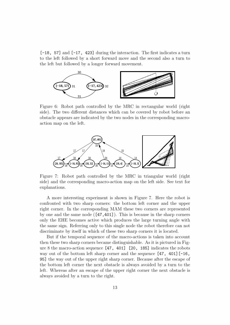
[-18, 57] and [-17, 423] during the interaction. The first indicates a turnto the left followed by a short forward move and the second also a turn tothe left but followed by a longer forward movement.

[−18, 57] 32[−17, 423]

31

30

31

Figure 6: Robot path controlled by the MRC in rectangular world (rightside). The two different distances which can be covered by robot before anobstacle appears are indicated by the two nodes in the corresponding macro-action map on the left.

[47, 401]

[20, 185] [−16, 95] [18, 32] [−16, 11] [18, 4] [−18, 3]

17 17 19 15

17 34 34 34 14 14

33

18 35 35 15 15

Figure 7: Robot path controlled by the MRC in triangular world (rightside) and the corresponding macro-action map on the left side. See text forexplanations.

A more interesting experiment is shown in Figure 7. Here the robot isconfronted with two sharp corners: the bottom left corner and the upperright corner. In the corresponding MAM these two corners are representedby one and the same node ([47,401]). This is because in the sharp cornersonly the EHE becomes active which produces the large turning angle withthe same sign. Referring only to this single node the robot therefore can notdiscriminate by itself in which of these two sharp corners it is located.

But if the temporal sequence of the macro-actions is taken into accountthen these two sharp corners became distinguishable. As it is pictured in Fig-ure 8 the macro-action sequence [47, 401] [20, 185] indicates the robotsway out of the bottom left sharp corner and the sequence [47, 401][-16,

95] the way out of the upper right sharp corner. Because after the escape ofthe bottom left corner the next obstacle is always avoided by a turn to theleft. Whereas after an escape of the upper right corner the next obstacle isalways avoided by a turn to the right.

13

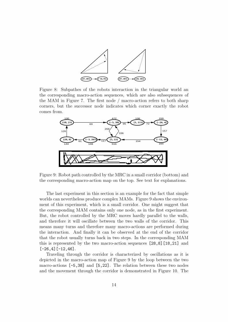
[47, 401] [−16, 95] [47, 401] [20, 185]

Figure 8: Subpathes of the robots interaction in the triangular world anthe corresponding macro-action sequences, which are also subsequences ofthe MAM in Figure 7. The first node / macro-action refers to both sharpcorners, but the successor node indicates which corner exactly the robotcomes from.

[−3, 265]

95

130

14461 117 154

516148

69

472

336

268

164

159

72

[5, 22]

[−5, 38] [−26, 4]

[−12, 46][28, 8]

[18, 21]

136

157126

[1, 111]

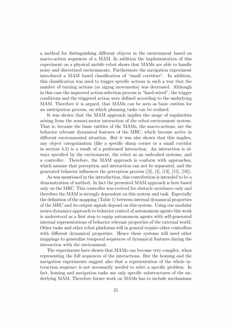
Figure 9: Robot path controlled by the MRC in a small corridor (bottom) andthe corresponding macro-action map on the top. See text for explanations.

The last experiment in this section is an example for the fact that simpleworlds can nevertheless produce complex MAMs. Figure 9 shows the environ-ment of this experiment, which is a small corridor. One might suggest thatthe corresponding MAM contains only one node, as in the first experiment.But, the robot controlled by the MRC moves hardly parallel to the walls,and therefore it will oscillate between the two walls of the corridor. Thismeans many turns and therefore many macro-actions are performed duringthe interaction. And finally it can be observed at the end of the corridorthat the robot usually turns back in two steps. In the corresponding MAMthis is represented by the two macro-action sequences [28,8][18,21] and[-26,4][-12,46].

Traveling through the corridor is characterized by oscillations as it isdepicted in the macro-action map of Figure 9 by the loop between the twomacro-actions [-5,38] and [5,22]. The relation between these two nodesand the movement through the corridor is demonstrated in Figure 10. The

14

[−5, 38] [5, 22]

Figure 10: Traveling through the small corridor is characterize by a zigzagmove, because the robot moves hardly parallel to the walls. So, the robot-environment interaction in this experiment is mainly described by small turn-ing angles followed by short straight forward moves. This is related to thesubstructure of the MAM in Figure 10 (bottom) with only two nodes andedges, because left and right turns are alternately performed.

most frequent occurrence of this oscillation in this experiment is indicatedby the large numbers of the corresponding nodes and edges in Figure 9.

[1, 111]

[−5, 38]

[5, 22]

Figure 11: In the MAM of the experiment with the small corridor (Fig. 9)the node [-5, 38] has the two successor nodes [5, 22] and [1, 111]. Thepaths which correspond to these macro-actions are shown, line style refers tothe same node / macro-action in the subgraph at the bottom of this figure.The two successor nodes or macro-actions are mainly distinguished by their”turning angles” 5 and 1. It is easy to see in this figure, that a smallerturning angle leads in a corridor to a longer straight forward movement.

Another point of the MAM in this experiment is, that the two nodes [-5,38] and [5, 22] representing the zigzag move through the corridor are theonly nodes, which have two successor nodes. It is easy to see in Figure 11 and12, that for each node the second successor node reflects the “experiences” ofthe robot, that in narrow corridors smaller turning angles to avoid collisionslead to longer straight forward movements.

15

[−5, 38]

[−3, 265]

[5, 22]

Figure 12: Like Figure 11, but according to node [5, 22] the successor node[-3, 265] in comparison with successor node [-5, 38] reflects the fact thatsmaller ”turning angles” lead to longer straight forward movements.

4.3 Experiments on Using MAMs for Exploration, Hom-

ing and Navigation

In the previous section the reader saw how MAM can be used to characterizethe robot–environment interaction. The next three experiments demonstratehow MAMs can be used to encode behavioral sequences, which overcome thelimited interaction of the MRC. In the following it is shown that a MAMbased categorization of environmental states can provide exploration, homingand navigation capabilities.

(a) (b) (c)

Figure 13: Robot path controlled by the MRC, but including a random turnif the last two (a) / four (b) / ten (c) macro-actions are similar. (100,000time steps are plotted in Fig. (a) and (b) and 250,000 in (c).)

First of all a few definitions must be introduced in this section. As itwas pointed out earlier, a MAM is a directed graph G = (V, E), with v ∈V representing the macro-actions and e ∈ E representing the predecessor-successor relationships between the macro-actions. A path of length k from amacro-action v0 to a macro-action vk in the directed graph G = (V, E) of theMAM is a sequence 〈v0, v1, . . . , vk〉 of macro-actions such that (vi, vi+1) ∈ E

for i = 0, . . . , k − 1. The length of the path is the number of relations. Wealso have to define the similarity of macro-actions and paths of macro-actions.Two macro-actions are similar (v0 ≈ v1) if they satisfy the relation given inequation 2. A path p of macro-actions is a subset of a MAM G = (V, E) if

16

∀ vp ∈ p ∃ vi ∈ V : vp ≈ vi and for each relation between to macro-actions inthe path, there exists a corresponding relation between two similar macro-action in the MAM. A corresponding relationship does not have to have thesame occurrence label; i.e.

p ⊂ G ⇐⇒ ∀ (vp, vp+1) ∈ p ∃ e = (vi, vi+1) ∈ E : vp ≈ vi, vp+1 ≈ vi+1, vi ∈ V.

The first experiment in this section demonstrates how the robot controlledby the MRC can develop an exploration behavior. We assume, that a goodexploration behavior is shown, if the robot’s path through the world coversup most of the free space. This is done using the square shaped environmentas shown in Figure 5. As it was already mentioned the robots interactionin this world is represented by a MAM with only one node and one edge.That means, during the interaction only one macro-action emerges. Duringthe interaction of the robot with the environment, a new path of macro-actions (in this case with vp = vq, ∀vp, vq ∈ p) is generated. To equip therobot with exploratory abilities the control of the interaction by the MRC isinterrupted, if a path p of a certain length k of newly recorded macro-actionsis a subset of the MAM. The interruption in this case means that the robotwill turn a random angle and then be controlled by the MRC again. Figure 13reflects the results of three experiments of this kind. The difference betweenthese three experiments is the value, which determines how many of the lastmacro-actions have to be similar before a random turn is triggered.

The results of the three experiments show that after the robot is rotatedby a random angle it does not take a long time to reach the old pathway, asshown in Figure 5. But in contrast to this figure the paths plotted in theFigures 13(a) – (c) indicate that there are two such stable pathways in thissquare shaped world. Depending from the start position and orientation therobot runs clockwise or counterclockwise through this world after a while.This determines in which of this two stable pathways the robot will end. Go-ing back to the exploration abilities, one can see that in all three experimentsthe robot covers the whole area. The difference is according to the length k

of the subset of macro-actions, that have to occur, before a random turn canbe performed.

In the next experiment a homing behavior using MAM was implemented.In a triangular world (like Figure 7) the robot has to recognize only one of thetwo sharp corners as its home and wait there for a while. As it was alreadyargued in the corresponding experiment of the pervious section, each sharpcorner in this world is represented by the same node in the MAM. Thereforethe robot has to distinguish the two sharp corners by a precedent sequenceof macro-actions. In detail, additionally to the pure MRC control a attention

17

mode is implemented, which is deactivated by default but becomes active, if aspecific sequence of two macro-actions occurs. Finally, if the attention modeis active and a macro-action corresponding to an extended hysteresis effect(EHE) occurs, then the robot stops for a certain time. After the waiting timeis over, the attention mode is deactivated and the robot is controlled again bythe MRC. Thus, “home” is not determined by the single node representingboth sharp corners but is distinguished by a macro-action sequence activatingthe attention mode. For example, if the upper right sharp corner is definedas “home” (compare Fig. 7), then a macro-action sequence similar to [47,

401][-16, 95] activates the attention mode. The sequence [47, 401][20,

185] defines the the bottom left corner as “home”.

Figure 14: Homing behavior experiment with the miniature robot Kheperain a triangular world, like Fig. 7. One of the two sharp corners in this worldis defined as home. If the robot moves in this ”home corner”, it has to staythere for a certain time.

This experiment has been done with a simulated and a real Kheperarobot testing each corner separately as home. A mpeg-video, which can bedownloaded from [10], shows two experiments with the real Khepera robot.Figure 14 is a screen shot of the first experiment in this movie where the”upper right” corner (according to Figure 7) is defined as home. Both exper-iments show the following fact: the robot only stops in the correct corner,but it also passes the correct corner. This is because, to recognize the sharpcorner, which is defined as home, a similar sequence of the correspondingmacro-action has to occur. In detail this means, that the robot can not takea look at the currently appearing sensor values, because they are ambiguous.In fact, a sequence or a path of macro-actions must be recorded in order tofind the correct corner. This means that a certain level of robot-environmentinteraction has to be performed, as the MRC has a limited sensory system.A robust discrimination between the two sharp corners can only be based onthe anticipated macro-action sequence, which emerge from a specific robot-environment interaction.

In the last experiment of this section the MAM is applied to solve anavigation problem. Figure 15(a) shows the path of a robot through a small

18

corridor, which is identical to the experiment in Fig. 9. As it was alreadymentioned in the pervious section, the movement through the corridor ismainly characterized by zigzag movements. But the MAM of this experimentreflects also ”experiences” of the robot that small turning angles lead tolonger distances before a new avoidance action has to be triggered. In thisexperiment it was tried to reduce the zigzag movements and bring the robotto straight movements through this corridor using the corresponding MAMin the following way.

(a)

(b)

(c)

Figure 15: Three robot paths through the small corridor. Figure (a) showsthe incisive zigzag movements of the robot. The two other figures show morestraight movements through the small corridor - mainly in the middle.

Like in the two experiments before the occurring macro-actions are mon-itored during the interaction. The control of the robot by the MRC is inter-rupted, if a macro-action occurs, which is similar to those macro-actions rep-resenting the oscillational behavior in the corridor (see Fig. 10). During thisinterruption the robot is turned 1 step to the right, if the last macro-action issimilar to [-5, 38]. This is defined according to its second successor node[1, 111] in the MAM (Fig. 9 and 11). Because this second successor noderefers to a longer distance before an avoidance behavior is triggered. Accord-ingly the robot is turned 3 steps to the left, if the last macro-action is similarto [5, 22]. Because in this case those 3 turn steps to the left refer to thesecond successor node [-3, 265] of node [5, 22] (Fig. 9 and 12), whichagain refers to a longer straight movement distance. After this rotation thecontrol is given back to the MRC.

Figure 15(b) and (c) show the results of two runs of this experiment. Thezigzag movements are still there, mainly at the ends of the corridor. Thisis not surprising, because first of all the specific macro-action must occur to”recognize” the small corridor and to trigger the smoother turns. In detail,

19

the dynamics of the controller has to be in or near enough to the correspond-ing attractor. But in the middle of the corridor straight movements are themajority. Whereas in the experiment, where the robot is only controlled bythe MRC (Fig. 15(a)), the zigzag movements are predominant.

5 Discussion

In this article a basic robot behavior - moving in a given environment byavoiding scattered objects - was chosen to demonstrate two methods forrepresenting robot-environment interactions by dynamical features of neuro-controllers. The first method, based on first return maps of sensori-motordata, revealed a clear difference in control techniques between a standardfeed-forward type of neuro-controller, the BC, and a more sophisticated one,the MRC, which makes extensive use of the recurrent connectivity of its mo-tor neurons. The resulting differences in robot behavior becomes obvious es-pecially in deadlock situations. In particular, the first return map (M-FRM)of the motor data and the combination (SMM) of sensor and motor dataappeared to be most instructive. They already indicate the existence of fourfundamental types of robot-environment interactions, which are constitutedby the neural structure of the MRC.

Based on Table 1 the MAMs can be seen to indicate the temporal sequenceof internal dynamical features of the MRC, which become effective during theinteraction of the robot with its environment. Basically each macro-actionfor the MRC relates to a hysteresis interval of sensor inputs followed bya dynamics determined by a global fixed point attractor. The number oftime steps of the actual rotation allows to distinguish between hysteresiseffects over small and extended input domains. Finally, the sign of a macro-action indicates left and right turns; i.e., left and right hysteresis effects.Therefore one can use the MAMs as a representation of the objects or specificfeatures of the world as they occur during the interaction of the robot withits environment. According to the four different dynamical properties of theMRC this representation can only refer to categories like obstacle on the left,obstacle on the right, deadlocks, and free space. This is an essential point,with respect to the landmark-based navigation approach. Landmark typesare defined by human designers [12] whereas the MAM approach only takesinto account the perception of the robot.

But the experiments in section 4 show that other categories of environ-mental conditions can be built, if substructures of MAMs are taken intoaccount. The experiments in section 4.3 indicated that MAMs can pro-vide homing and navigation tasks. The homing experiment demonstrated

20

a method for distinguishing different objects in the environment based onmacro-action sequences of a MAM. In addition the implementation of thisexperiment on a physical mobile robot shows that MAMs are able to handlenoisy and discretized environments. Furthermore the navigation experimentintroduced a MAM based classification of “small corridors”. In addition,this classification was used to trigger specific actions in such a way that thenumber of turning actions (or zigzag movements) was decreased. Althoughin this case the improved action-selection process is “hard-wired”, the triggerconditions and the triggered action were defined according to the underlyingMAM. Therefore it is argued, that MAMs can be seen as basic entities foran anticipation process, on which planning tasks can be realized.

It was shown that the MAM approach implies the usage of regularitiesarising from the sensori-motor interaction of the robot-environment system.That is, because the basic entities of the MAMs, the macro-actions, are thebehavior relevant dynamical features of the MRC, which become active indifferent environmental situation. But it was also shown that this implies,any object categorization (like a specific sharp corner or a small corridorin section 4.3) is a result of a performed interaction. An interaction is al-ways specified by the environment, the robot as an embodied systems, anda controller. Therefore, the MAM approach is conform with approaches,which assume that perception and interaction can not be separated, and thegenerated behavior influences the perception process ([3], [4], [13], [15], [19]).

As was mentioned in the introduction, this contribution is intended to be ademonstration of method. In fact the presented MAM approach is here basedonly on the MRC. This controller was evolved for obstacle avoidance only andtherefore the MAM is strongly dependent on this system and task. Especiallythe definition of the mapping (Table 1) between internal dynamical propertiesof the MRC and its output signals depend on this system. Using our modularneuro-dynamics approach to behavior control of autonomous agents this workis understood as a first step to equip autonomous agents with self-generatedinternal representations of behavior relevant properties of the external world.Other tasks and other robot platforms will in general require other controllerswith different dynamical properties. Hence these systems will need othermappings to generalize temporal sequences of dynamical features during theinteraction with the environment.

The experiments have shown that MAMs can become very complex, whenrepresenting the full sequences of the interactions. But the homing and thenavigation experiments suggest also that a representation of the whole in-teraction sequence is not necessarily needed to solve a specific problem. Infact, homing and navigation tasks use only specific substructures of the un-derlying MAM. Therefore future work on MAMs has to include mechanisms

21

which can focus on or separate relevant substructures of the MAM.But the question which substructures of a MAM or which internal repre-

sentation of the environment will be necessary and sufficient for the agent isthen of course task dependent. Therefore the agent must be able to evaluatethe MAM by itself with respect to a given problem or task. Following [6]we argue, that this evaluation of the agents internal representation has toinclude the agents anticipated and the actual interaction outcomes. The el-ements of the MAM are directly related to the external world and accessibleby the agent and therefore a promising starting point to endow autonomousagents with self-generated internal representation to improve their behavioralrepertoire.

References

[1] Angeline, P.J., Saunders, G.B. and Pollack J.B. (1994), An EvolutionaryAlgorithm that Evolves Recurrent Neural Networks, IEEE Transactionson Neural Networks, 5, 54-65.

[2] Arbib, M.A., Erdi, P. and Szentagothai, J. (1998), Neural Organization:Structure, Function, and Dynamics, Cambridge, MA, MIT Press.

[3] Bajcsy, R. (1988), Active Perception, Proceedings of the IEEE, 76: 996– 1005, 1988.

[4] Ballad, D.H. (1991), Animate vision, Artificial Intelligence, 48:57 – 86.

[5] Beer, R., (1995) A dynamical systems perspective on agent-environmentinteraction, Artificial Intelligence, 72(1), pp. 173 – 215, 1995.

[6] Bickhard, M. H., Treveen, L. (1995) Foundational Issues in ArtificialIntelligence and Cognitive Science, Elsevier Scientific, Amsterdam, 1995.

[7] Braitenberg, V. (1984), Vehicles: Experiments in Synthetic Psychology,MIT Press, Cambridge, MA.

[8] Harnard, S. (1990), The symbold grouding problem, Physica D, 42, pp.335–346.

[9] Hulse, M., Pasemann, F. (2001), Dynamical Neural Schmitt Triggerfor Robot Control, J. R. Dorronsoro(Ed.): ICANN 2002, LNCS 2415,Springer Verlag Berlin Heidelberg New York, pp. 783–788, 2002.

22

[10] Hulse, M.: Implementation of homing behavior based on a re-current neuro-controller and macro-action maps, MPEG video,http://www.ais.fraunhofer.de/INDY/aml/X/MRChoming.mpeg,12.12.2002.

[11] Krichmar, J. L., Edelman, G. M., (2002), Machine Psychology: Au-tonomous Behavior, Perceptual Categorization, and Conditioning in aBrain-Based Device, Cerebral Cortex, vol. 12, pp. 818 – 830, 2002.

[12] Mataric, M.J. (1994), Navigating With a Rat Brain: ANeurobiologically-Inspired Model for Robot Spatial Representa-tion, Proceedings of the International Conference on Simulation ofAdaptive Behavior: From Animals to Animats 3, 282–290, 1994.

[13] Metta, G., Fitzpatrick, P. (2002), Better Vision Through Manipulation,In: Proceedings of the Second International Workshop on EpigeneticRobotics: Modeling Cognitive Developement in Robotic Systems, Prince,C. G., Demiris, Y., Marom, Y., Kozima, H. and Balkenius, C. (Eds.),Lund University Cognitive Studies, 94, 97 – 104, 2002.

[14] Michel, O., Khepera Simulator Package version 2.0: Freeware mobilerobot simulator written at the University of Nice Sophia-Antipolis byOliver Michel. Downloadable from the World Wide Web at http://

wwwi3s.unice.fr/ ∼om/ khep-sim.html

[15] Moller, R. (1999), Perception Through Anticipation - A Behavior-BasedApproach to Visual Perception. In: Understanding Representation in theCognitive Sciences (A. Riegler; A. von Stein; M. Peschl, eds.), PlenumPress, New York, 1999.

[16] Mondada, F., Franzi, E., Ienne, P. (1993), Mobile robots miniaturiza-tion: a tool for investigation in Control Algorithms. In Proceedings ofISER’ 93, Kyoto, October 1993.

[17] Mondada, F., Floreano, D. (1995), Evolution of neural control struc-tures: Some experiments on mobile robots. Robotics and AutonomousSystems, 16:183 – 195.

[18] Nolfi, S., Floreano, D. (2000), Evolutionary Robotics: The Biology, Intel-ligence, and Technology of Self-Organizing Machines, MIT Press, Cam-bridge.

[19] Nolfi, S., Marocco, D., Active Perception: A Sensorimotor Account ofObject Categorization, Proceedings of the 7th International Conference

23

on Simulation of Adaptive Behavior: From Animals to Animats 7, 266–271, 2002.

[20] Pasemann, F. (1993), Dynamics of a single model neuron, InternationalJournal of Bifurcation and Chaos, 2, 271–278.

[21] Pasemann, F. (1995), Neuromodules: A dynamical systems approachto brain modelling. In Herrmann, H., Poppel, E. and Wolf, D. (eds.),Supercomputing in Brain Research - From Tomography to Neural Net-works, Signapore: World Scientific, pp. 331-347.

[22] Pasemann, F. (1995), Characteristics of periodic attractors in neuralring networks, Neural Networks, 8, 421-429.

[23] Pasemann, F., Steinmetz, U., Hulse, M., and Lara, B. (2001), Robotcontrol and the evolution of modular neurodynamics, Theory in Bio-sciences, 120, 311–326.

[24] Tani, J. (1998), An Interpretation of the “Self” From the Dynamical Sys-tems Perspective: A Constructivist Approach, Journal of ConsciousnessStudies, 5(5-6), 1998.

[25] Tani, J., Sugita, Y. (1999), On the Dynamics of Robot ExplorationLearning, Proc. of 5th European Conf. of Artificial Life (ECAL99), 279-288, 1999.

[26] Wolpert, D.M., Ghahramani, Z., Flanagan, J.R. (2001), Perspectivesand problems in motor learning, Trends in Cognitive Science, 5(11):487-494.

24