Embed Size (px)
Citation preview

Technical Report Documentation Page 1. Report No. FHWA/TX-02/1819-1
2. Government Accession No.
3. Recipient's Catalog No.
4. Title and Subtitle EVALUATION OF SUPERPAVE SHEAR TEST PROTOCOLS
5. Report Date January 2002
6. Performing Organization Code
7. Author(s) Arif Chowdhury and Joe Button
8. Performing Organization Report No. Report 1819-1 10. Work Unit No. (TRAIS)
9. Performing Organization Name and Address Texas Transportation Institute The Texas A&M University System College Station, Texas 77843-3135
11. Contract or Grant No. Project No. 0-1819 13. Type of Report and Period Covered Research: September 1999-August 2001
12. Sponsoring Agency Name and Address Texas Department of Transportation Research and Technology Implementation Office P. O. Box 5080 Austin Texas 78763-5080
14. Sponsoring Agency Code
15. Supplementary Notes Research performed in cooperation with the Texas Department of Transportation and the US Department of Transportation, Federal Highway Administration. Research Project Title: Evaluation of Shear Strength Property of HMAC for Predicting Performance 16. Abstract
The Strategic Highway Research Program (SHRP) study, during the development of the Superpave mixture design and analysis process, provided a series of test protocols using the Superpave shear tester (SST) to predict the performance of the hot mix asphalt (HMA) mixtures. Excessive time is required to conduct all of these test procedures on each HMA mixture designed, which can significantly increase the cost of mixture design. Conducting all of the tests can be confusing and even conflicting. The objective of this study is to evaluate four selected Superpave shear test protocols and determine which of the test protocols is most suitable for predicting asphalt pavement performance. The predominant pavement performance of interest herein is rutting. So, the ultimate goal is to identify the “best” SST test protocol that can evaluate the shearing resistance of HMA.
Researchers selected or developed four different mixtures from very poor to excellent quality using materials from Texas and Georgia. The HMA mixtures selected for this study were: Type C limestone, Type D rounded river gravel, granite stone mastic asphalt (SMA), and granite Superpave. Rutting performance of these mixtures was evaluated using four SST protocols: Frequency Sweep at Constant Height (FSCH), Simple Shear at Constant Height (SSCH), Repeated Shear at Constant Height (RSCH), and Repeated Shear at Constant Stress Ratio (RSCSR). Three laboratory-scale accelerated loaded wheel tests were performed on these four mixtures to compare the results with those from the SST. The loaded wheel tests used in this study were: Asphalt Pavement Analyzer, 1/3-Scale Model Mobile Load Simulator, and Hamburg Wheel Tracking Device.
Researchers recommended the FSCH test as the “best” SST protocol. To determine the precision of the FSCH test, compacted specimens from three HMA mixtures were sent to six different laboratories across the US to conduct an interlaboratory test program.
17. Key Words SST, Mixture Characterization, APA, Hamburg, MMLS3, Shear Resistance
18. Distribution Statement No restrictions. This document is available to the public through NTIS: National Technical Information Service 5285 Port Royal Road Springfield, Virginia 22161
19. Security Classification (of this report) Unclassified
20. Security Classification (of this page) Unclassified
21. No. of Pages 112
22. Price
Form DOT F 1700.7 (8-72) Reproduction of completed page authorized


EVALUATION OF SUPERPAVE SHEAR TEST PROTOCOLS
by
Arif Chowdhury Associate Transportation Researcher
Texas Transportation Institute
and
Joe Button Senior Research Engineer
Texas Transportation Institute
Report 1819-1 Project Number 0-1819
Research Project Title: Evaluation of Shear Strength Property of HMAC for Predicting Performance
Sponsored by the Texas Department of Transportation
In Cooperation with the US Department of Transportation Federal Highway Adminstration
January 2002
TEXAS TRANSPORTATION INSTITUTE The Texas A&M University System College Station, Texas 77843-3135


v
DISCLAIMER
The contents of this report reflect the views of the authors, who are responsible for the
facts and the accuracy of the data presented herein. The contents do not necessarily reflect the
official view or policies of the Federal Highway Administration (FHWA) or the Texas
Department of Transportation (TxDOT). This report does not constitute a standard,
specification, or regulation. The engineer in charge was Joe W. Button, P.E., (Texas, # 40874).

vi
ACKNOWLEDGMENTS
The work reported herein was conducted as part of a research project sponsored by the
Texas Department of Transportation and the Federal Highway Administration.
The researchers gratefully acknowledge the support and guidance of Mr. Richard Izzo of
TxDOT, project director of this research project, and Mr. Maghsoud Tahmoressi, who initiated
this project as the original project director. Researchers appreciate Mr. Andre Smit for helping
during the loaded wheel testing at the TxDOT facility. The contributions of Mr. Shekhar Shah,
graduate research assistant for this project, are highly appreciated.
Special thanks are extended to Martin Marietta Technologies, Young Brothers paving
contractor for providing several thousand pounds of aggregate, and Koch Materials, Inc. for
providing necessary asphalt at no cost to this project.

vii
TABLE OF CONTENTS
Page List of Figures ................................................................................................................................. x List of Tables ................................................................................................................................. xi Chapter 1: Introduction .................................................................................................................. 1
Background................................................................................................................................. 1 Problem Statement ...................................................................................................................... 2 Objective ..................................................................................................................................... 3 Scope of the Report..................................................................................................................... 3
Chapter 2: Literature Review.......................................................................................................... 5 General........................................................................................................................................ 5
Hveem Stability Testing ........................................................................................................ 5 Marshall Stability and Flow Testing ..................................................................................... 6 Superpave Shear Tester ......................................................................................................... 7
Uniaxial, Volumetric, Simple Shear Test......................................................................... 8 Frequency Sweep Test...................................................................................................... 8 Repeated Shear Test ......................................................................................................... 8
Evaluation of Superpave Shear Tester................................................................................... 9 Unconfined Compressive Strength Test .............................................................................. 10 Uniaxial Creep Test ............................................................................................................. 10 Resilient Modulus Test........................................................................................................ 11 Dynamic Complex Modulus Test........................................................................................ 11 NCHRP Project 9-19 ........................................................................................................... 12
Dynamic Modulus .......................................................................................................... 12 Flow Number.................................................................................................................. 12 Flow Time ...................................................................................................................... 13
Full-Scale Test Track........................................................................................................... 13 Laboratory-Scale Accelerated Tests ......................................................................................... 14
Georgia Loaded-Wheel Tester ....................................................................................... 14 Asphalt Pavement Analyzer ........................................................................................... 15 Hamburg Wheel Tracking Device.................................................................................. 16 Model Mobile Load Simulator - 1/3 Scale ..................................................................... 17 French Wheel Tracker .................................................................................................... 18 Purdue University Laboratory Wheel Tester.................................................................. 19
Chapter 3: Experimental Design................................................................................................... 21 Plan of Study............................................................................................................................. 21 Materials Selection and Acquisition ......................................................................................... 22
Type C Limestone Mixture ................................................................................................. 22 Type D River Gravel Mixture ............................................................................................. 22 Granite SMA Mixture.......................................................................................................... 24 Granite Superpave Mixture ................................................................................................. 24 Tests for Asphalt Cement Characterization......................................................................... 25
Dynamic Shear Rheometer............................................................................................. 25 Bending Beam Rheometer (BBR) .................................................................................. 26

viii
Page
Direct Tension Tester (DTT).......................................................................................... 27 Rotational Viscometer .................................................................................................... 27 Mixing and Compaction Temperature............................................................................ 27
Tests for Aggregate Characterization .................................................................................. 28 Coarse Aggregate Angularity (CAA)............................................................................. 29 Fine Aggregate Angularity (FAA) ................................................................................. 29 Flat and Elongated Particles (F&E)................................................................................ 30 Clay Content ................................................................................................................... 31
Superpave Shear Tester............................................................................................................. 31 Description of Equipment.................................................................................................... 32
Testing Apparatus........................................................................................................... 32 Control and Data Acquisition System ............................................................................ 33 Environmental Control Unit ........................................................................................... 34 Hydraulic System ........................................................................................................... 34
Specimen Preparation and Instrumentation......................................................................... 34 Description of Tests .................................................................................................................. 36
Volumetric Test .............................................................................................................. 36 Uniaxial Test .................................................................................................................. 37 Frequency Sweep Test at Constant Height..................................................................... 37 Simple Shear at Constant Height Test............................................................................ 39 Repeated Shear at Constant Height Test ........................................................................ 40 Repeated Shear at Constant Stress Ratio Test ................................................................ 42
Accelerated Wheel Testing ....................................................................................................... 44 Asphalt Pavement Analyzer ................................................................................................ 44 1/3 Scale - Model Mobile Load Simulator .......................................................................... 46
MMLS3 Test Specification ............................................................................................ 47 TxDOT MMLS3 Testing Facility .................................................................................. 47 Compaction of Test Pad ................................................................................................. 48 MMLS3 Test Setup ........................................................................................................ 48 Temperature Control ...................................................................................................... 49 Profilometer Measurements and Rutting Definition ...................................................... 50
Hamburg Wheel Testing Device ......................................................................................... 52 Chapter 4: Results and Discussions .............................................................................................. 55
General...................................................................................................................................... 55 Superpave Shear Tester............................................................................................................. 55
Frequency Sweep at Constant Height.................................................................................. 55 Complex Shear Modulus ................................................................................................ 56 Shear Phase Angle.......................................................................................................... 58
Simple Shear at Constant Height......................................................................................... 59 Maximum Shear Strain................................................................................................... 60 Permanent Shear Strain .................................................................................................. 60 Elastic Recovery............................................................................................................. 61
Repeated Shear at Constant Height ..................................................................................... 63 Repeated Shear at Constant Stress Ratio............................................................................. 65

ix
Page
Mixture Rankings by SST Protocols ................................................................................... 66 Results from Loaded Wheel Testers ......................................................................................... 68
Asphalt Pavement Analyzer ................................................................................................ 68 Model Mobile Load Simulator - 1/3 Scale .......................................................................... 70
Limestone ....................................................................................................................... 71 River Gravel ................................................................................................................... 71 Granite SMA .................................................................................................................. 72 Granite Superpave .......................................................................................................... 73 Slab Density ................................................................................................................... 73
Hamburg Wheel Tracking Device....................................................................................... 74 Mixture Rankings by Loaded Wheel Testers ...................................................................... 77
Selection of “Best” SST Test Protocol ..................................................................................... 77 Chapter 5: Interlaboratory Testing................................................................................................ 83
General...................................................................................................................................... 83 Chapter 6: Conclusions and Recommendations ........................................................................... 85
General...................................................................................................................................... 85 Conclusions............................................................................................................................... 85
Superpave Shear Testing ..................................................................................................... 85 Accelerated Loaded Wheel Testing..................................................................................... 86
Recommendations..................................................................................................................... 87 References..................................................................................................................................... 89 Appendix: Material Characterization............................................................................................ 95

x
LIST OF FIGURES Page Figure 1. Gradations of Mixtures Used in Study........................................................................ 23 Figure 2. Cox Superpave Shear Tester....................................................................................... 33 Figure 3. Superpave Gyratory Compactor ................................................................................. 36 Figure 4. Shear Strain and Axial Stress Pulses in the FSCH Test.............................................. 38 Figure 5. Typical Stress Application for the SSCH Test. .......................................................... 40 Figure 6. Stress Pulses in the RSCH Test. ................................................................................. 41 Figure 7. Permanent Defromation versus Repeated Load Applications. ................................... 42 Figure 8. Stress Pulses in the RSCSR Test. ............................................................................... 43 Figure 9. Asphalt Pavement Analyzer........................................................................................ 45 Figure 10. APA Test Setup........................................................................................................... 45 Figure 11. Schematic of the MMLS3........................................................................................... 46 Figure 12. Schematic of MMLS3 Test Setup............................................................................... 49 Figure 13. Adjustments to Vertical Transverse Surface Profiles. ................................................ 51 Figure 14. Profilometer Used to Measure MMLS3 Rut Depth.................................................... 52 Figure 15. Hamburg Wheel Tracking Device Mold..................................................................... 53 Figure 16. HWTD Loaded with Specimens. ................................................................................ 53 Figure 17. Complex Shear Modulus at 39°F................................................................................ 56 Figure 18. Complex Shear Modulus at 68°F................................................................................ 57 Figure 19. Complex Shear Modulus at 104°F.............................................................................. 57 Figure 20. Shear Phase Angle versus Frequency at 39°F. ........................................................... 58 Figure 21. Shear Phase Angle versus Frequency at 68°F. ........................................................... 58 Figure 22. Shear Phase Angle versus Frequency at 104°F. ......................................................... 59 Figure 23. Maximum Shear Strain for Different Mixtures. ......................................................... 62 Figure 24. Permanent Shear Strain for Different Mixtures .......................................................... 62 Figure 25. Elastic Recovery of Different Mixtures...................................................................... 63 Figure 26. Permanent Shear Strain from RSCH Test................................................................... 64 Figure 27. Permanent Shear Strain from RSCSR Test................................................................. 66 Figure 28. Rut Depth Measured by APA ..................................................................................... 69 Figure 29. Comparison of Mean Cummulative Rutting (APA) ................................................... 69 Figure 30. Zoom of a Typical MMLS3 Wheelpath Rut Measurement ........................................ 70 Figure 31. Cumulative Rutting on Limestone Mixture ................................................................ 71 Figure 32. Cumulative Rutting on River Gravel Mixture ............................................................ 72 Figure 33. Cumulative Rutting on Granite SMA Mixture ........................................................... 72 Figure 34. Cumulative Rutting on Granite Superpave Mixture ................................................... 73 Figure 35. Comparison of Mean Cumulative Rutting for All Mixtures (MMLS3) ..................... 74 Figure 36. Rut Depth Produced by HWTD at 10,000 Cycles (TxDOT)...................................... 76 Figure 37. Comparison of Mean Cumulative Rutting (HWTD-TxDOT) .................................... 76 Figure A1. Viscosity-Temperature Relationship of PG 64-22 Asphalt ........................................ 99 Figure A2. Viscosity-Temperature Relationship of PG 76-22 Asphalt ..................................... 100

xi
LIST OF TABLES Page Table 1. Gradations of Four Mixtures....................................................................................... 23 Table 2. Mixture Design Information. ...................................................................................... 24 Table 3. Mixing and Compaction Temperatures ...................................................................... 28 Table 4. Coarse Aggregate Angularity Test Results................................................................. 29 Table 5. Fine Aggregate Angularity Test Results..................................................................... 30 Table 6. Flat and Elongated Aggregate Test Results ................................................................ 31 Table 7. Clay Content Test Results........................................................................................... 31 Table 8. Frequencies, Number of Cycles Applied, and Data Points per Cycle ........................ 39 Table 9. Test Condition and Specimen Description for the Different Mixtures....................... 54 Table 10. Stress Level Applied in the SSCH Test ...................................................................... 60 Table 11. SSCH Test Result ....................................................................................................... 61 Table 12. Mixture Rankings by FSCH Test ............................................................................... 66 Table 13. Mixture Rankings by SSCH Test................................................................................ 67 Table 14. Mixture Rankings by Repeated Shear Tests ............................................................... 68 Table 15. Final Rut Depth Measured by APA............................................................................ 68 Table 16. MMLS3 Slab Density ................................................................................................. 74 Table 17. Final Rut Depth Produced by HWTD at TxDOT ....................................................... 75 Table 18. Final Rut Depth Produced by HWTD at TTI.............................................................. 76 Table 19. Mixture Ranking by Accelerated Wheel Testers ........................................................ 77 Table 20. CV of Mixture Properties Determined by the FSCH Test at 10 Hz Cycle ................. 79 Table 21. CV of Mixture Properties Determined by the SSCH Test.......................................... 79 Table 22. CV of Mixture Properties Determined by the Two Repeated Shear Tests ................. 80 Table 23. CV of Mixture Properties Determined by the Loaded Wheel Testers........................ 80 Table 24. Duncan Grouping of the FSCH Results...................................................................... 81 Table 25. Duncan Grouping of the SSCH Results...................................................................... 81 Table 26. Duncan Grouping of the Two Repeated Shear Tests Results ..................................... 81 Table 27. Duncan Grouping of the Loaded Wheel Tests Results ............................................... 82 Table A1. PG 64-22 Test Results and Requirements .................................................................. 97 Table A2. PG 76-22 Test Results and Requirements .................................................................. 97

xii

1
CHAPTER 1:
INTRODUCTION
BACKGROUND
Permanent deformation or rutting is a major issue for hot mix asphalt (HMA) pavements
throughout the nation. Texas is no exception. Under a recent National Cooperative Highway
Research Program (NCHRP) study (1), researchers conducted a national survey and found that
rutting was overwhelmingly the most important HMA pavement distress. The main contributors
to increased rutting observed in the last decade appear to be higher truck tire pressures and axle
loads and increased truck traffic (2). Truck tire pressure has been increased from 70-80 psi to
120-140 psi in the past 20 years. As a result, the top pavement layer (HMA) is subjected to more
and higher stresses and is thus more susceptible to rutting. A 1987 study (3) suggests that truck
tire pressure will continue to increase. Therefore, the best technology available must be used to
design and construct HMA pavements to ensure they are capable of carrying this increasing
traffic load.
Approximately 94 percent of paved roads in Texas are asphalt pavements. Each year,
rehabilitation of these existing roads and construction of new roads require about 12 million tons
of HMA. District pavement engineers, area engineers, and laboratory supervisors are constantly
faced with decisions regarding selection of the best asphalt mixture design to use in construction
or rehabilitation of particular pavement. Texas Department of Transportation (TxDOT) and
contractors need to have a method available that is capable of verifying that the selected mixture
design is not likely to exhibit premature distress during service under the anticipated traffic
loading, temperature regime, and pavement substrate. Rutting, the major form of premature
distress, is caused mainly by insufficient shearing strength of HMA (4). Therefore, a laboratory
test method that can verify a mixture’s shearing strength and, hence, the rutting resistance would
be extremely valuable to not only TxDOT but also to all highway specifying agencies and
contractors who are required to warranty pavement performance.

2
PROBLEM STATEMENT
During the early 1990s under the Strategic Highway Research Program (SHRP) study,
development of the Superpave mixture design and analysis process provided a series of test
protocols with various test conditions. Superpave volumetric mixture design alone does not
provide adequate warranty against pavement distresses like permanent deformation and or
fatigue cracking. To ensure better resistance to different kinds of distresses, SHRP introduced
the intermediate (Level II) and complete (Level III) mixture design and analysis system, which
depend on traffic level. The Superpave Shear Tester (SST) was introduced as a component of
the Superpave mixture design and analysis system to perform all load-related performance tests.
This testing device is capable of using both static and dynamic loading in confined and
unconfined conditions. Initially, SHRP researchers proposed six different SST test protocols to
characterize HMA. The six different tests were as follows:
• Volumetric Test,
• Uniaxial Test,
• Frequency Sweep at Constant Height (FSCH) Test,
• Simple Shear at Constant Height (SSCH) Test,
• Repeated Shear at Constant Height (RSCH) Test, and
• Repeated Shear at Constant Stress Ratio (RSCSR) Test.
These six test procedures measure several engineering properties. Due to lack of time,
SHRP researchers could not determine which of the test protocol/protocols were best suited for
predicting the rutting performance of HMA. Excessive time is required to conduct all of these
test procedures on each asphalt mixture designed. American Association of State Highway and
Transportation Officials (AASHTO) Standard TP 7-94 (5) calculates the time required for level
III and Level II test protocols as 111 and 58 hours, respectively. Level III and Level II require
21 and 12 HMA specimens, respectively, to conduct the tests with the SST. Excessive time
required to perform these tests can significantly increase the cost of mixture design. Conducting
all of the tests can be confusing and even conflicting.

3
It is desirable to evaluate these Superpave shear test protocols in a systematic
experimental program to determine which engineering property is most suitable to for predicting
the shearing strength or rutting susceptibility of HMA.
A recent survey under NCHRP Project 9-19 shows that HMA industries prefer a
relatively simple and low-cost equipment to characterize the HMA (1). When this study began,
test requirements for the SST were complex and expensive. The most readily apparent methods
for simplifying the SST equipment appear to involve elimination of the confining pressure. If
the SST protocols requiring confining pressure (volumetric test and uniaxial test) prove to
correlate more poorly with pavement performance than the other SST protocols, then the large
compressor and air seals could be eliminated and the strength requirements of the chamber could
be greatly reduced. This is one way to simplify and lower the cost of the equipment. After this
study began, AASHTO eliminated the volumetric and uniaxial tests from the SST protocols.
OBJECTIVE
The objective of this study is to evaluate the four remaining Superpave shear test
protocols developed by SHRP researchers to determine which of the test protocols is most
suitable for predicting asphalt pavement performance. The predominant pavement performance
of interest is rutting. So, the ultimate goal will be to identify the “best” suited SST test protocol
that can evaluate the shearing resistance of hot mix asphalt.
The secondary objective is to simplify the SST equipment. In fact, if the identified “best”
test protocol does not involve confining pressure, the exclusion of the confining chamber will
automatically simplify and reduce the cost of the equipment. Other objectives include
developing acceptance criteria and a precision statement for the “best” SST protocol.
SCOPE OF REPORT
This report is divided into six chapters. Chapter 1 serves as an introduction, stating the
nature of the problem to be addressed, objectives of the research, and scope of work
accomplished.
Chapter 2 summarizes an overview of HMA mixture evaluation techniques with an
emphasis on the permanent deformation. It covers the different test methods used in last decades
to identify the rutting resistance of HMA. This literature review describes mechanistic,

4
empirical, and accelerated pavement testing. This chapter provides information on HMA
shearing strength evaluation procedures and their relationship to pavement performance.
Chapter 3 is a description of the experimental program. The work plan includes the
following tasks: planning of study, materials selection and acquisition, testing to characterize
asphalt cement and aggregates, mixture design and/or calibration, and testing to evaluate asphalt
concrete mixtures. HMA evaluation tests include tests with the SST, Asphalt Pavement
Analyzer (APA), 1/3-Scale Model Mobile Load Simulator (MMLS3), and Hamburg Wheel
Tracking Device (HWTD).
Chapter 4 covers analysis of the results from different tests that have been conducted to
evaluate the shearing resistance of different HMA mixtures. This chapter includes the results
and analysis of SST tests and other laboratory-scale rutting tests. This chapter includes
comparative analysis of results from SST and other laboratory-scale rutting tests.
Chapter 5 presents results of the interlaboratory study of the Frequency Sweep at
Constant Height test, which was found to be the “best” SST test protocol. FSCH tests were
conducted at four regional Superpave Centers, Asphalt Institute (AI), and Federal Highway
Administration (FHWA). This chapter presents the precision statement for the “best” test
protocol determined on the basis of the interlaboratory test study.
Chapter 6 presents conclusions and recommendations that arose from the study. Detailed
results of some tests are discussed in the appendix.

5
CHAPTER 2: LITERATURE REVIEW
GENERAL
HMA material characterization was introduced in the early twentieth century. Many test
methods were developed during last century. Some of them are empirical test methods and
correlated poorly with field performance. Many of the test methods have become obsolete. In
this study, researchers concentrated on the test methods used for characterizing the shearing
properties of HMA. Currently, the Superpave volumetric mixture design procedure lacks a basic
design criterion to evaluate fundamental engineering properties of the asphalt mixture that
directly affects performance (1).
Hveem Stability Testing
In late 1920s, Francis Hveem of the then California Highway Department developed the
Hveem stabilometer. The purpose of this testing was to measure the stability of highway
materials under various states of confinement (6). This brilliant test was developed as an
empirical measure of internal friction within a mixture (7). Later, this stability test for asphalt
mixture was standardized in American Society for Testing and Materials (ASTM) D 1560 and
AASHTO T 246.
The Hveem stability tester applies a vertical axial load on a 4-inch (102 mm) diameter by
2.5-inch (64 mm) high HMA specimen in a confined stress condition using a rubber membrane.
It measures the resulting horizontal pressure and displacement at an applied vertical pressure of
400 psi (2760 kPa) at 140°F (60°C). This temperature is designed to simulate the most critical
yet typical filed condition. Hveem stability of asphalt concrete is calculated using the following
equation:
222.0
2.22
hv
h +−
=
PPDP
S ,
where, S = Hveem stability number of asphalt concrete,
D = displacement of the specimen,

6
Pv = vertical pressure applied (400 psi), and
Ph = horizontal pressure gauge reading in psi.
Different agencies slightly modified the testing procedure and the equation. The stability value
of fluid will be near zero as Pv ≅ Ph. Whereas, the stability value of steel will be near 100 as Ph
approaches zero.
Researchers also developed a companion test using the cohesiometer to measure cohesion
or the tensile characteristics of HMA. The cohesiometer was rarely used, as the testing error is
very high and there is little correlation between the test result and actual performance. Although
widely used for many years, Hveem stability testing itself is not highly correlated with the field
performance.
Marshall Stability and Flow Testing
Bruce Marshall developed the Marshall asphalt concrete mixture design while working
for the Mississippi Highway Department in the late 1930s. Later, the U.S. Army Corps of
Engineers modified the Marshall mixture design system. As part of the mixture design system,
strength of the asphalt mixture is determined using the Marshall stability and flow tester to
determine optimum asphalt content. It has also been used for quality control. This test, to
determine the relative potential of a mixture to exhibit instability, was later standardized as
ASTM D 1559 and AASHTO T 245.
The Marshall test apparatus applies a vertical compressive load on the cylindrical surface
of a specimen using two semicircular testing heads. The specimen is 4 inches (102 mm) in
diameter by 2.5 inches (63.5 mm) high and is compacted in a specified manner. The test is
conducted at 140°F (60°C) and rate of loading is 2 inches (50 mm) per minute. This temperature
is a critical yet practical field condition. This apparatus provides two materials indicators:
stability and flow.
Marshall stability is the maximum load sustained by the specimen before failure. The
Marshall flow value is the total vertical deformation (in 0.01 inches [0.025 mm]) of the specimen
at maximum load. Higher stability values indicate stronger mixtures. Sometimes another
property called Marshall stiffness index (ratio between Marshall stability and Marshall flow
number) is used to characterize mixtures.
7
It is believed that a mixture with higher a stability number or higher Marshall stiffness
index will be resistant to permanent deformation or rutting. There is very little correlation data
between Marshall stability number and actual field performance of HMA mixtures (7).
Superpave Shear Tester
To improve the performance, durability, and safety of United States roads, Congress
established SHRP in 1987 as a 5-year research program. Fifty million dollars of the one hundred
and fifty million dollars of the SHRP research funds were used for the development of asphalt
specifications to directly relate laboratory analysis with field performance. SuperpaveTM was the
final product of the SHRP research effort. Superpave is a complete mixture design and analysis
system with three major components: asphalt binder specification,
mixture design methodology, and analysis system.
Under the mixture design and analysis part of the SHRP research, researchers developed
two devices to quantify the performance of an HMA mixture. They are the Superpave Shear
Tester and the Indirect Tensile Tester. Initially, researchers proposed six test protocols using the
SST to characterize the permanent deformation and fatigue resistance of HMA mixtures.
Permanent deformation and fatigue are both load-related distresses. In this study, researchers
will concentrate on the permanent deformation characterization only.
During the SHRP study, several universities were included in a team formed to select test
methods to characterize the permanent deformation property of HMA mixtures (8). This team
developed the SST machine. This machine measures some basic material properties responsible
for permanent deformation: nonlinear elastic property, Vermeer plastic property, viscoelastic
property, and tertiary creep property (9). The SST can provide material constitutive relations
necessary for mechanistic road response models (6). The original intent of many of these tests
was that they would be used as input into performance models developed during SHRP (10).
Despite successful application in the research field, most of the tests, material properties, and
theoretical models are not currently in common use by the industry. The six SST test protocols
to measure the permanent deformation characteristics of HMA mixtures are presented below.
Chapter 3 discusses further details of these test protocols.

8
Uniaxial, Volumetric, Simple Shear Test
These three test methods measure the nonlinear elastic property and Vermeer plastic
property. Only one load cycle (static) is applied in these tests. Basically, they are load-unload
tests. All three tests involve loading a test specimen at a specified controlled stress magnitude,
holding the load for a specified time, and unloading the test specimen at a specified rate (9).
Uniaxial and volumetric tests use confining pressure, while the simple shear test does not. The
loadings of the specimens are designed to imitate field conditions.
During the loading and unloading process, the specimens are subjected to elastic and
plastic strain. From the elastic part of the stress-strain graph, two major material properties are
calculated: elastic modulus and Poisson’s ratio. The plastic part provides a volumetric constant,
peak angle of friction, factor related to the cohesive shear strength, and friction angle at constant
volume. All of these materials properties are predicators of rutting of HMA mixtures.
Frequency Sweep Test
Frequency sweep is a strain-controlled repeated test that is used to measure the
viscoelastic behavior of asphalt mixtures. A small magnitude of sinusoidal shearing strain is
applied on the specimen at 10 different frequencies, and the stress response is measured. Due to
the viscoelastic behavior of an HMA mixture, the specimen’s stress response is not in the same
phase as the applied strain. The stress is always lagging behind the applied strain. The ratio
between the stress response and the applied strain is used to compute the complex shear
modulus. The measured time delay between the strain and stress response is used to compute
shear phase angle.
Higher complex modulus indicates a stiffer mix that is more resistant to rutting. Lower
shear phase angle indicates more elastic behavior that is more resistant to rutting.
Repeated Shear Test
There are two types of repeated shear tests: constant height and constant stress. The
objective of developing these tests was to find a check for an HMA mixture’s susceptibility to
tertiary creep. Tertiary creep is a severe form of rutting where a small number of load repetition
can cause a large amount of plastic deformation. Tertiary creep indicates gross instability of the
mixture.

9
A large number of repeated loads is applied in both cases, and the shearing deformation is
measured. In a constant stress test, repeated synchronized haversine shear and axial load pulses
are applied to the specimen. Each load pulse is followed by a rest period. The ratio of haversine
axial load to shear load is maintained at a constant ratio within the range of 1.2 to 1.5. The
repeated shear load shear at constant stress ratio was included in the Superpave method as a
screening test to identify mixtures that exhibit tertiary plastic flow, indicating instability and
leading to premature rutting (11).
In the constant height test, a haversine shear load of a specified magnitude is applied on
the specimen, and a variable axial load is applied to keep the specimen height constant. Each
load pulse is followed by a rest period.
Evaluation of Superpave Shear Tester
Romero and Mogawer (12) conducted a research study to determine if the results from
the SST could be used to differentiate the properties of five laboratory-prepared asphalt mixtures
without the need for any models. They analyzed the properties obtained from the SST and
compared them with the performance of the respective mixtures tested at the Accelerated
Loading Facility (ALF) at FHWA. They examined the FSCH, SSCH, and RSCH tests. Some of
their conclusions were: the trends observed in most SST tests were consistent with the ALF
performance, the complex shear modulus at 104°F (40°C) obtained from the FSCH test was able
to discern good and bad mixtures, RSCH test results were extremely variable, shear modulus
ranking matched with ranking from the ALF, and elastic strain from the SSCH test was not able
to discern among the mixtures.
Tayebali et al. (13) conducted a study to evaluate the performance of the RSCH test.
They examined three field mixtures and tested using the RSCH test, Georgia Loaded Wheel
Tester (GWLT), and French Rut Tester (FRT). When comparing with field rutting performance
(after several years of service), the researchers found that the RSCH test can clearly identify the
well-performing versus poor-performing mixtures.
Stuart and Izzo (14) compared the G*/sin δ of five binders (note: not mixtures) tested
using the dynamic shear rheometer (DSR) with the results from HMA mixtures tested using the
GLWT, HWTD, and FRT. They observed that G*/sin δ correlates very well with results from
the GLWT and reasonably correlates with the results from the HWTD and FRT.

10
Anderson et al. (10) documented the SST performance of various asphalt mixtures tested
at Asphalt Institute since 1994. The objective of that study was to create a database to provide
guidance to the users indicating how a project’s asphalt mixture compares to other mixtures with
performance history.
Anderson et al. (15) presented a case history on Specific Pavement Study No. 9 (SPS-9).
To showcase the Superpave system, four SPS-9 pilot projects were built in the summer of 1992.
Reviewing the field performance of those sections after 7 years of service and comparing the
laboratory test results on those mixtures, the authors concluded that two SST tests, SSCH and
FSCH, correctly ranked the observed pavement rutting performance.
Shenoy and Romero (16) suggested a procedure to unify the sets of curves generated
from the FSCH tests performed at various temperatures on different mixtures. The procedure
involves the use of a normalizing frequency parameter. They also proposed that the temperature
at which the normalizing parameter becomes equal to 1.0 could be considered as a specification
parameter for assessing mixture performance. Researchers determined the specification
parameter for various mixtures of known performance and found it to follow the performance
rankings in all studied cases.
Unconfined Compressive Strength Test
The unconfined compressive strength test procedure to evaluate the strength of asphalt
concrete has been widely used by the pavement industry (6). This test is a standardized test in
ASTM D 1074 and AASHTO T 167. In this test, a fixed or monotonic axial load is applied on a
cylindrical specimen at a steady rate until the specimen fails. The peak load divided by the cross-
sectional area is referred to as the unconfined compressive strength of the mixture. The specimen
size is 4 inches (100 mm) in diameter and 8 inches (200 mm) in height. There is little evidence
that the field rutting performance correlates with the unconfined compressive strength.
Uniaxial Creep Test
The uniaxial creep test has been used for many years to estimate the rutting potential of
HMA mixtures. The creep test may involve either static or repeated haversine load. In both
cases, an axial load is applied on the cylindrical specimen and the resulting permanent
deformation with time is measured. The total plastic strain induced during a creep test is
recorded and plotted as function of the logarithm time or load applications. Typical creep

11
behavior of asphalt concrete is composed of (1) primary densification, (2) steady-state creep, and
(3) a tertiary creep phase. Using the creep test data in the VESYS software, one can predict the
rut depth progression of a pavement by assuming permanent vertical strain is directly
proportional to the resilient strain (6).
Uniaxial creep test data can be used to evaluate the permanent deformation potential of
asphalt concrete mixtures when the laboratory creep testing is performed in such a manner as to
simulate realistic field stress conditions (17).
Resilient Modulus Test
Resilient modulus is one of the most common methods of measuring HMA mixture
stiffness. In this test procedure, a repeated haversine axial load is applied on the cylindrical
surface of a specimen (similar to the indirect tension test). The specimen is not loaded to failure;
rather, it is loaded to a stress level between 5 and 20 percent of normal strength. The standard
test procedure can be obtained from ASTM D 4123. There is no good correlation between
modulus of resilience and rutting (7). This is no surprise, since by definition, the test does not
produce shear strain in the specimen. Results typically correlate strongly with binder
characteristics but not with aggregate characteristics.
Dynamic Complex Modulus Test
Dynamic complex modulus of an HMA mixture is determined by applying sinusoidal
compressive stress along the axis of a cylindrical specimen. The standardized test procedure is
presented in ASTM D 3497. Researchers developed this test during the 1960s. According to the
ASTM procedure, the height-to-diameter ratio should be 2:1 to sufficiently minimize the effect
of friction and resulting shearing stress at the top and bottom of the specimen. The most
common specimen size is 4 inches (100 mm) × 8 inches (200 mm). The applied load usually
ranges up to 35 psi (241.5 kPa). Tests are usually conducted usually at three different
temperatures and three different frequencies. Typical temperatures are 41, 77, and 104°F (5, 25,
and 40°C), and the loading frequencies are 1, 4, and 16 Hz.
The dynamic complex modulus is calculated by dividing the repeated vertical stress by
the resulting repeated axial strain. The primary purpose of measuring dynamic modulus was to

12
determine the stress-strain relationship. This test has limited use because of long testing time,
complexity and cost of equipment, and large specimen size (7).
NCHRP Project 9-19
During the late 1990s, FHWA established NCHRP Project 9-19. The objectives of the
NCHRP project are to “(1) develop simple performance tests for permanent deformation and
fatigue cracking for incorporation in the Superpave volumetric mix design method, and (2)
develop and validate an advanced material characterization model and the associated calibration
and testing procedures for hot mix asphalt used in highway pavements” (18). Under this project,
Dr. Matt Witczak and his co-workers proposed “some simple performance tests” to evaluate the
permanent deformation of HMA mixtures. They are as follows.
Dynamic Modulus
The dynamic modulus test procedure is similar to ASTM D 3497 with some
modifications. In the proposed test method, dynamic modulus (E*) and phase angle (N) are
measured from the sinusoidal axial load application on a cylindrical Superpave Gyratory
Compactor (SGC) specimen at a single temperature (Teff = 77 to 140°F [25 to 40°C]) and design
loading frequency (0.1 to 10 Hz). Here, the complex modulus is calculated by dividing the stress
by the axial strain. The phase angle is the angle lagging by the axial strain from the axial stress.
The concept is similar to the FSCH test by SST equipment. The specimen used for this test is 4
inches (100 mm) in diameter and 6 inches (150 mm) in height. Witczak, et al. (1) reported
excellent correlations between E*/sin φ and rutting performance from certain test tracks and
the FHWA-ALF.
Flow Number
Flow number is the number of load repetitions at which shear deformation begins under
constant volume. In this test protocol, the SGC compacted cylindrical specimen is subjected to
repetitive axial load in a triaxial environment at a single temperature (Teff = 77 to 140°F [25 to
40°C]). The load is applied for a duration of 0.1 s, followed by a rest period of 0.9 s. Usually, a
10-30 psi (69-207 kPa) stress is applied and the cumulative permanent axial and radial strains are
recorded throughout the test. The specimen dimension is the same as that of the dynamic

13
modulus test. Witczak et al. (1) reported from good to excellent correlations between flow
number and rutting performance from certain test tracks and the FHWA-ALF.
Flow Time
Flow time is defined as the postulated time when shear deformation starts under constant
volume. In this test protocol, the SGC compacted cylindrical specimen is subjected to static
axial load in a triaxial environment at a single temperature (Teff = 77 to 140°F [25 to 40°C]). The
applied stress and the resulting permanent axial and radial strains are recorded throughout the
test to calculate the flow time. Witczak et al. (1) reported from good to excellent correlations
between flow time and rutting performance from certain test tracks and the FHWA-ALF.
Full-Scale Test Track
Several different test tracks have been constructed since the 1960s to evaluate a wide
variety of pavement parameters. Some test tracks have been built to serve specific purposes.
Some of the test tracks constructed and tested so far include:
• AASHO Road Test
• University of Illinois Test Track
• MnRoad
• WesTrack
• NCAT Test Track
These test tracks are also capable of mixture material characterization. Usually, this type
of test pavement is constructed with several different test sections. Full-scale loaded trucks
with/without drivers are operated continuously on the test pavements, and the distresses are
measured at regular intervals. A huge number of load repetitions is required to simulate field
conditions. This type of mixture characterization is probably the best method to simulate field
conditions. The two major problems with this method are, of course, cost and time. That is why
test tracks are limited only for major research purposes.

14
LABORATORY-SCALE ACCELERATED TESTS
For the last two decades, the use of laboratory-scale wheel testers to estimate the rutting
potential of HMA mixture has become more popular. Most of the wheel testers estimate rutting
susceptibility of asphalt mixtures by applying repeated wheel passes in a comparatively short
period and usually employ an elevated temperature to accelerate the damage. Many
transportation agencies and pavement industrial firms have begun using loaded wheel testers
(LWT) to supplement their mixture design procedure (19). Several studies mention the use of
loaded-wheel testers (19, 20, 21, 22, 23, 24, 25).
The LWTs provide an accelerated evaluation of rutting potential in their HMA mixtures.
LWTs enable asphalt mixtures and pavement structures to be evaluated in a fraction of time
required for normal trafficking. The accelerated pavement tester (APT) can be full-scale or
scaled-down to some degree. According to Metcalf (26), the full-scale APT should have
controlled application of a prototype wheel loading, at or above the appropriate legal load limit,
to a prototype or actual layered, structural pavement system to determine pavement response and
performance under a controlled, accelerated accumulation of damage in a compressed time
period. This acceleration of damage can be achieved by means of increased repetitions, modified
loading condition, and imposed climatic conditions, or a combination of those factors. The
overall idea is to simulate, as closely as possible, a real-life situation.
Contrary to full-scale APT, model or laboratory APT does not attempt to model real-
world conditions but rather manipulates these conditions directly and/or artificially to evaluate
the critical performance parameters of materials and structures in an accelerated time frame.
Controlling variables such as pavement temperatures, base stiffness, aging influence, moisture
condition, loading conditions, and fundamental failure mechanisms may be induced in a fraction
of time and cost compared to full-scale testing under real-world conditions. Following is a short
description of several loaded-wheel testers used in the USA.
Georgia Loaded-Wheel Tester
Georgia Department of Transportation and Georgia Institute of Technology jointly
developed the GLWT device in the mid-1980s (19, 27). This machine could be mentioned as a
pioneer of laboratory-scale loaded wheel testers in the USA. Rut testing of HMA specimens is
accomplished by applying a 100-lb (445 N) aluminum wheel load onto a pneumatic hose

15
pressurized to 100 psi (690 kPa). This pressurized hose applies a load directly on the specimens.
Usually 8000 cycles of repeated (forward and backward) wheel loads are applied to the
specimens. The device will accept either cylindrical or beam specimens. Rolling wheel
compactors, vibratory compactors, or the Superpave gyratory compactor can accomplish
compaction of specimens. Field cores or slab specimens can also be used. Typically, the air
void contents of the test specimens are 4 percent or 7 percent. Test temperature of the GLWT
ranges from 95 to 140°F (35 to 60°C).
Several studies showed the GLWT is capable of ranking the mixtures similar to the field
rutting performance (19, 28, 29).
Asphalt Pavement Analyzer
The APA is basically a modified and improved version of the GLWT. Operation of the
APA is similar to that of the GLWT. By far, the APA is the most popular and commonly used
loaded wheel tester in the USA. Pavement Technology, Inc. started manufacturing this
equipment from the mid-1990s. The APA is capable of evaluating rutting, fatigue, and moisture
resistance of HMA mixtures. The fatigue test is performed on beam specimens supported on the
two ends. Rutting and moisture-induced damage evaluations can be performed on either
cylindrical or beam specimens. This machine is capable of testing in both dry and wet
conditions.
Oscillating beveled aluminum wheels apply a repetitive load through high-pressure hoses
to generate the desired contact pressure. The loaded wheel oscillates back and forth over the
hose. While the wheel moves in the forward and backward directions, the linear variable
differential transducers (LVDTs) connected to the wheels measure the depression at regularly
specified intervals. Usually, three replicates of specimens are tested in this machine. Rut
evaluation is typically performed by applying 8000 load cycles. The wheel load is usually 100 lb
(445 N), and the hose pressure is 100 psi (690 kPa). Some researchers have successfully used
this device with higher wheel load and contact pressure (30). APA testing can be performed
using chamber temperatures ranging 41 to 160°F (5 to 71°C) (31).
Several research projects have been conducted to evaluate performance of the APA.
Choubane et al. (24) indicated that the APA might be an effective tool to rank asphalt mixtures in
terms of their respective rut performance. Kandhal et al. (25) reported that the APA has the

16
ability to predict relative rutting potential of HMA mixtures. They also mentioned that the APA
is sensitive to asphalt binder and aggregate gradation. Uzarowski and Emery (32) found good
correlations between the rutting resistance predicted by the APA and actual field performance of
asphalt concrete pavements.
Hamburg Wheel Tracking Device
The Hamburg wheel tracking device (HWTD) is an accelerated wheel tester. Helmut-
Wind, Inc. in Hamburg, Germany, originally developed this device (20). It has been used as a
specification requirement for some of the most traveled roadways in Germany to evaluate rutting
and stripping (19). Use of this device in the USA began during the 1990s. Several agencies
undertook research efforts to evaluate the performance of the HWTD. The Colorado Department
of Transportation (CDOT), FHWA, National Center for Asphalt Technology (NCAT), and
TxDOT are among them.
Since the adoption of the original HWTD, significant changes have been made to this
equipment. A U.S. manufacturer now builds a slightly different device. The basic idea is to
operate a steel wheel on a submerged, compacted HMA slab or cylindrical specimen. The
original HWTD uses a slab with dimensions of 12.6 inches × 10.2 inches × 1.6 inches (320 mm
× 260 mm × 40 mm). The slab is usually compacted at 7 ± 1 percent air voids using a linear
kneading compactor. The test is conducted under water at constant temperature ranging from 77
to 158°F (25 to 70°C). Testing at122°F (50°C) is the most common practice (19). The sample
is loaded with a reciprocating motion of the 1.85-inch (47 mm) wide steel wheel using a 158-lb
force (705 N). Usually, the test is conducted at 20,000 cycles or up to a specified amount of rut
depth. Rut depth is measured at several locations including the center of the wheel travel path,
where usually it reaches the maximum value. One forward and backward motion comprises two
cycles.
Precision Metal Works, a Kansas-based company, now manufactures a HWTD. Their
device is slightly different and improved from the original version. This device is capable of
testing with both slab and cylindrical specimens. The HWTD measures rut depth, creep slope,
stripping inflection point, and stripping slope (19). The creep slope is the inverse of the
deformation rate within the linear range of the deformation curve after densification and prior to
stripping (if stripping occurs). The stripping slope is the inverse of the deformation rate within

17
the linear region of the deformation curve after the stripping takes place. The creep slope relates
primarily to rutting from plastic flow, and the stripping slope indicates accumulation of rutting
primarily from the moisture damage (22). The stripping inflection point is the number of wheel
passes corresponding to the intersection of creep slope and stripping slope.
Tim Aschenbrener (20) found an excellent correlation between the HWTD and
pavements with known field performance. He mentioned that this device is sensitive to the
quality of aggregate, asphalt cement stiffness, length of short-term aging, refining process or
crude oil source of the asphalt cement, liquid and hydrated lime anti-stripping agent, and
compaction temperature.
Izzo and Tahmoressi (22) conducted a repeatability study of the HWTD. Seven different
agencies took part in that study. They experimented with several different versions of the
HWTD. They used both slab and Superpave gyratory compacted specimens. Some of their
conclusions were the device yielded repeatable results for mixtures produced with different
aggregates and with test specimens fabricated by different compacting devices, and cylindrical
specimens compacted with the SGC are acceptable for moisture susceptibility evaluation of
different mixtures.
Model Mobile Load Simulator – 1/3 Scale
The MMLS3 was introduced as a scaled-down accelerated pavement testing device for
use in a controlled environment (33). Researchers developed the MMLS3 by scaling down from
the full-scale Texas Mobile Load Simulator (19, 34). It is used for testing scale-model pavement
sections or test pads. This machine has been used successfully on actual roadways. The
MMLS3 has four single tires in series, linked together to form an endless chain. Each wheel is
attached to a 1-foot diameter pneumatic tire. The wheels move around a set of looped rails in the
vertical plane on a fixed frame and apply loads to a short section of pavement. Some of the
advantages of this type of APT device are that the load is always moving in one direction, many
repetitions are possible in a short period of time, and a relatively high trafficking speed is
possible.
The wheels can be laterally displaced across a 6-inch (150 mm) wide path in a normal
distribution about the centerline to simulate traffic wandering. The tires may be inflated up to a
pressure of 120 psi (800 kPa). Axle loads varying between 470 and 600 lb (2100 and 2700 N)

18
are possible. The axle loads are automatically kept constant at a predetermined value by the
special suspension system. Nominal wheel speed is 8.2 ft/s (2.5 m/s), applying about 7200 load
cycles per hour. A single variable-speed motor drives the chain of four wheels. Typical number
of cycles used for the testing is between 100,000 and 200,000.
The MMLS3 can be used to evaluate the asphalt pavement sections in wet and dry
conditions. An environmental chamber surrounding the machine is used for elevating the
temperature. The test temperature can be increased up to 140°F (60°C). Performance monitoring
during MMLS3 testing includes measuring the rut depth from transverse profiles at multiple
locations of the wheelpath. Currently, there is no standard procedure for this test method.
At Stellenbosch University, South Africa, researchers are examining the ability of the
MMLS3 to predict the fatigue behavior of HMA mixtures. They are using Superpave gyratory
compacted specimens for this purpose. Research studies by the TxDOT used the MMLS3 to
determine the relative performance of two rehabilitation processes and establish the predictive
capability of this device (19). Comparison of pavement responses under full-scale Texas Mobile
Load Simulator and the scaled-down MMLS3 showed good correlation when researchers
considered actual loading and environmental conditions.
French Wheel Tracker
The Laboratoire Central des Ponts et Chausees developed the French Wheel Tracker, also
known as the FRT, during the 1970s and 1980s (35). Recently, the Colorado Department of
transportation and FHWA, at their Turner Fairbank Highway Research Center, conducted a
research program to evaluate the performance of the FRT (19).
The test specimen is an asphalt slab with typical dimensions of 7.1 inches × 19.7 inches
(180 mm × 500 mm). The FRT can apply wheel loads simultaneously on two test slabs.
Loading is accomplished by applying a 1125-lb (5000 N) wheel load using a smooth pneumatic
tire pressurized at 87 psi (600 kPa). The pneumatic tire passes over the slab center at the rate of
120 times per minute. For rut susceptibility evaluation, the test is conducted at a higher
temperature range, typically 122 to 140°F (50 to 60°C).
FRT rut depth is defined by the deformation expressed as a percentage of the original
slab thickness. The rut depth is measured across the width of the specimen. The typical number
of cycles used with the FRT is 6000 (34).

19
Purdue University Laboratory Wheel Tracking Device
This device, also known as “PURWheel,” was developed at Purdue University. The
device was designed as a flexible general-purpose tester (36). It is capable of evaluating rutting
potential and/or moisture sensitivity of HMA (19). In this device, load is applied on compacted
test slab through a pneumatic tire.
The slab specimens are usually 11.4 inches (290 mm) wide and 12.2 inches (310 mm)
long. The thickness varies from 1.5 to 3 inches (38 to 75 mm), depending on the type of
mixture. The linear kneading compactor developed at Purdue University accomplishes
compaction of laboratory specimens. A typical range of specimen air voids is 6 to 8 percent.
The wheel load and tire contact pressure are 385 lb (1713 N) and 90 psi (620 kPa), respectively.
The test environment can be hot/wet or hot/dry. Test temperature can range from room
temperature to 149°F (65°C).
During testing, rutting is measured across the wheelpath. The PURWheel is typically
operated for 20,000 wheel passes or until 0.8 inch (20 mm) of rutting has occurred. Moisture
sensitivity of HMA mixtures is defined as the ratio of the number of cycles required for 0.5-inch
(12.7 mm) rut depth in a wet condition to the number of cycles required for 0.5-inch (12.7 mm)
rut depth in a dry condition.


21
CHAPTER 3:
EXPERIMENTAL DESIGN
PLAN OF STUDY
All six of the SST protocols are intended to characterize the load-related behavior of
HMA. During the inception of this research study, all of the six SST protocols were under
consideration. Later in the study, TxDOT and the researchers were informed of AASHTO’s
decision to discontinue three of the SST protocols. In the AASHTO provisional standard,
Interim Guide for April 2001, only three tests were recommended; they are Simple Shear at
Constant Height, Frequency Sweep at Constant Height, and Repeated Shear at Constant Height.
The logic behind discontinuing the volumetric and uniaxial tests was due to the complexity of
the test procedures, complexity of the test setups, and inconsistency of the test results. AASHTO
also stated that the repeated shear at constant stress ratio test does not provide any new property
that repeated shear at constant height test cannot provide. Researchers of this study and TxDOT
readily accepted elimination of the volumetric test and uniaxial test. But the researchers wanted
to examine all four of the other test protocols. The test plan is divided into the four following
steps:
• Materials selection and acquisition: This step includes identification of four HMA
mixtures with different rutting properties and collection of the aggregate, asphalt, and
other components to produce those mixtures.
• Asphalt cement and aggregate characterization: The individual HMA mixture
components were tested to determine if they meet Superpave requirements.
• Mixture design and verification: One new mixture was designed and three other
mixture designs borrowed from other agencies were verified in the laboratory.
• Asphalt concrete mixture evaluation: Performance tests to establish rut resistance of
the HMA mixtures were performed. Performance tests of HMA included the
Superpave Shear Tester and Asphalt Pavement Analyzer, 1/3-Scale MMLS, and
Hamburg Wheel Tracking Device.

22
MATERIALS SELECTION AND ACQUISITION
Researchers and the former project director, Mr. Tahmoressi, in the project kick-off
meeting, identified four HMA mixtures with known or predictable field performance. Ideally,
these four mixtures should exhibit field performance (particularly related to rutting) from
excellent to poor. The reason for setting such criteria for the candidate mixtures was to examine
the relative sensitivity of the SST and other HMA-characterizing test methods. The HMA
mixtures selected for this study were: Type C limestone, Type D rounded river gravel, granite
stone mastic asphalt (SMA), and granite Superpave. These mixtures were developed in Texas
and Georgia. Once TTI researchers received the mixture design and mixture constituents,
specimens were compacted using the respective design methods to verify the optimum asphalt
content. In some cases, minor modifications (changes in asphalt content) were necessary to
achieve the desired air void content. Table 2 summarizes the four mixture designs used in this
study. The following paragraphs provide a brief description of these mixtures.
Type C Limestone Mixture
This HMA mixture was originally designed at Colorado Materials Company located in
San Marcos, Texas. Colorado Materials Company supplied this mixture to several districts for
numerous projects. The districts primarily using this mixture are San Antonio, Yoakum, Austin,
Corpus Christi, and Bryan. The overall subjective rating of field performance of this mixture is
good. The aggregates used for this mixture are Colorado Type C, Colorado Type D, Colorado
Type F, Colorado manufactured sand, and Colorado field sand. All aggregates were collected
from Colorado Materials except the field sand. The field sand was collected from Bryan, Texas.
The asphalt used in the research study was PG 64-22, supplied by Koch Materials, Inc. Since the
materials source was slightly different from the original source, the mixture design was checked
in the laboratory and the optimum asphalt content was found to be 4.4 percent instead of 4.6
percent. Table 1 and Figure 1 present the mixture design gradation. From now on, this Type C
limestone mixture will be referred to as the limestone mixture.
Type D River Gravel Mixture
This HMA mixture was designed at the TTI laboratory to obtain a rut-susceptible
mixture. The aggregates were collected from the local Brazos River valley. This mixture uses
mostly uncrushed and rounded river gravel and field sand. PG 64-22 asphalt was used in this
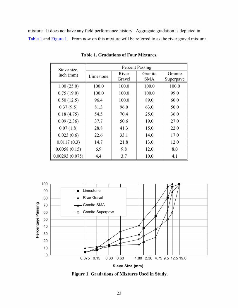
23
mixture. It does not have any field performance history. Aggregate gradation is depicted in
Table 1 and Figure 1. From now on this mixture will be referred to as the river gravel mixture.
Table 1. Gradations of Four Mixtures.
Percent Passing Sieve size, inch (mm) Limestone River
Gravel Granite SMA
Granite Superpave
1.00 (25.0) 100.0 100.0 100.0 100.0 0.75 (19.0) 100.0 100.0 100.0 99.0 0.50 (12.5) 96.4 100.0 89.0 60.0 0.37 (9.5) 81.3 96.0 63.0 50.0
0.18 (4.75) 54.5 70.4 25.0 36.0 0.09 (2.36) 37.7 50.6 19.0 27.0 0.07 (1.8) 28.8 41.3 15.0 22.0
0.023 (0.6) 22.6 33.1 14.0 17.0 0.0117 (0.3) 14.7 21.8 13.0 12.0
0.0058 (0.15) 6.9 9.8 12.0 8.0 0.00293 (0.075) 4.4 3.7 10.0 4.1
Figure 1. Gradations of Mixtures Used in Study.
19.012.59.54.752.361.800.600.300.150.0750
10
20
30
40
50
60
70
80
90
100
Sieve Size (mm)
Perc
enta
ge P
assi
ng
Limestone
River Gravel
Granite SMA
Granite Superpave

24
Granite SMA Mixture
This SMA mixture is usually considered to be a very rut-resistant mixture. Georgia
Department of Transportation (DOT) provided this mixture design. They use this mixture on
their heavy-duty pavements. The mixture was designed using 50 blows of the Marshall hammer.
The granite aggregate used for the mix design was obtained from a Vulcan Materials quarry in
Lithia Springs, Georgia. PG 76-22 asphalt, supplied by Koch Materials, Inc., was used in this
mixture. In addition to granite aggregate, 0.4 percent mineral fiber, 1.0 percent lime, and 9.0
percent fly ash were used in the mixture. Boral Materials Technology provided the fly ash. To
produce the same gradation as the original design, researchers at TTI fractionated all aggregates
into different ASTM standard sieve sizes and recombined them in accordance with mixture
design. The purpose of using the mineral fiber is to prevent drain down of liquid asphalt mastic
from the mixture.
During verification of the mix design, the optimum asphalt content was reduced to 5.9
percent from 6.1 percent (original optimum asphalt content). Table 1 and Figure 1 illustrate the
design aggregate gradation.
Table 2. Mixture Design Information.
Mixture Type Binder Content (%)
Binder Type
Rice Density (gm/cc)
Design Method
Limestone 4.4 PG 64-22 2.428 Texas Gyratory River Gravel 5.5 PG 64-22 2.416 Texas Gyratory Granite SMA 5.9 PG 76-22 2.396 Marshall 50-blow Granite Superpave 4.0 PG 64-22 2.481 Superpave
Granite Superpave Mixture
Georgia DOT also provided this 19.0-mm Superpave mixture design. The idea behind
selecting this mixture was to obtain a mixture with very good rut resistance. In Georgia, this
mixture is known as “Level B.” The aggregate for this mixture has the same source as the
granite SMA mixture. The filler includes 1.0 percent hydrated lime. During the mix design
process, the number of SGC gyrations used are 7, 86, and 134, as Ninitial, Ndesign, and Nmaximum ,
respectively. PG 64-22 asphalt was used for this mixture. In fact, the same asphalt was used in

25
the limestone, river gravel, and granite Superpave mixtures. During the mixture verification
process at the TTI laboratory, the optimum asphalt content was increased to 4.0 percent instead
of the original 3.9 percent. The aggregate for this mixture was sieved to different size fractions
and recombined to obtain an accurate gradation. Aggregate gradation is shown in Table 1 and
Figure 1.
Tests for Asphalt Cement Characterization
One of the three major components of the Superpave mixture design process is the
asphalt binder performance grading specification (AASHTO MP1). Asphalt binder is tested
under conditions that simulate its critical stages during service in a pavement, such as:
• during transportation, storage, and handling - original binder is tested;
• during mix production and construction - simulated by short-term aging the original
binder in a rolling thin film oven (RTFO); and
• after 5 to 10 years of service - simulated by long-term aging the binder in the rolling
thin film oven test plus the pressure aging vessel (PAV).
The appendix includes results of the binder tests.
Dynamic Shear Rheometer
Researchers used the DSR to characterize viscous and elastic behavior of asphalt binders
at high and intermediate service temperatures. The DSR measures the complex shear modulus
(G*) and phase angle (δ) of asphalt binders at the desired temperature and frequency of loading.
Complex modulus is a measure of the total resistance of a material to deformation when
repeatedly sheared. It consists of two components:
• storage modulus (G′) or the elastic (recoverable) part, and
• loss modulus (G″) or the viscous (nonrecoverable) part.
The lag time between the applied peak stress and resulting peak strain is the phase angle
(δ). For perfectly elastic materials, the phase angle is 0 degrees, and, for perfectly viscous fluid

26
materials, it is 90 degrees. Asphalt binders behave like elastic solids at very low temperatures
and like viscous fluids at high temperatures. However, at typical pavement service temperatures,
asphalt behaves like a viscoelastic material; therefore, δ will be greater than zero but smaller than
90 degrees (7).
The DSR is used to determine the rutting parameter of the asphalt binder at high
temperatures for unaged binders and short-term aged binders. For rutting resistance, a high
complex shear modulus (G*) value and low phase angle (δ) are both desirable. Higher G*
values indicate stiffer binders that are more resistant to rutting. Lower δ values indicate more
elastic asphalts that are more resistant to rutting. Therefore, a larger G*/sin δ signifies more
resistance to permanent deformation by the asphalt binder.
The DSR is also used to determine the fatigue resistance of the asphalt binder at
intermediate temperatures for long-term aged binders. For fatigue resistance, a low complex
modulus value and a low phase angle are both desirable. Therefore, smaller values of G*sin δ
should indicate more resistance to fatigue cracking.
Bending Beam Rheometer (BBR)
The BBR measures a binder’s resistance to thermal cracking. Thermal cracking may
occur in asphalt pavements when the temperature drops rapidly at low temperatures. The BBR
uses a transient creep-bending load on the center of an asphalt cement beam specimen held at a
constant low temperature. This test is performed on asphalt binder that has been subjected to
long-term aging. From this test, two parameters are obtained:
• creep stiffness - a measure of how the asphalt binder resists the constant creep
loading, and
• m-value - a measure of the rate at which the creep stiffness changes with
time of loading.
If creep stiffness increases, the thermal stresses developed in the pavement due to thermal
shrinking also increase and thermal cracking becomes more likely. If m-value decreases (the
curve flattens), the ability of the asphalt binder to relieve thermal stresses decreases and the
propensity for thermal cracking increases.

27
Direct Tension Tester (DTT)
The DTT measures the low-temperature ultimate tensile strain of the binder. This test is
performed using binder that has been subjected to long-term aging. The DTT is used only when
the asphalt creep stiffness obtained from the BBR is greater than 300 MPa but smaller than 600
MPa. The DTT is used because there are some asphalt binders that may have high creep stiffness
but do not crack because they can stretch farther before breaking. Larger failure strain indicates
more ductile binders and, therefore, more resistant to cracking.
Rotational Viscometer
The rotational viscometer (often referred as the Brookfield viscometer) was adopted in
Superpave for determining the viscosity of asphalt binder at high temperatures, primarily to
ensure that it is sufficiently fluid for pumping or mixing. Rotational viscosity is determined by
measuring the torque required to maintain a constant rotational speed of a cylindrical spindle.
The rotational viscometer determines optimum HMA mixing and compaction temperatures.
Mixing and Compaction Temperature
Superpave HMA mixtures are mixed and compacted under equiviscous temperature
conditions corresponding to 0.17 Pa•s and 0.28 Pa•s, respectively (4). Viscosity of the asphalt
was tested using the Brookfield rotational viscometer at 275°F (135°C) and 347°F (175°C).
Plotting the result on a viscosity versus temperature graph (log-normal), the mixing and
compaction temperatures were determined for PG 64-22 asphalt. But applying the same
procedure unusually yielded excessive mixing and compaction temperatures for PG 76-22
asphalt. Therefore, the mixing and compaction temperatures used for the PG 76-22 were those
suggested by the supplier. Table 3 describes the mixing and compaction temperatures for both
asphalts.
Details of binder testing and the results and determination of the mixing and compaction
temperatures are described in the Appendix.

28
Table 3. Mixing and Compaction Temperatures.
Mixing Compaction Asphalt Grade Temp Range
(°F) Selected Temp,
(°F) Temp Range, (°F) Selected Temp, (°F)
PG 64-22 317 - 330 320 294 - 306 295 PG 76-22 315 - 335 330 280 - 310 310
Tests for Aggregate Characterization
Superpave specifications contain two categories of aggregate properties: consensus
properties and source properties (4). Consensus properties are those aggregate characteristics
that are critical to well-performing asphalt mixtures. These properties include:
• coarse aggregate angularity,
• fine aggregate angularity,
• flat and elongated particles, and
• clay content.
The specific criteria for these consensus aggregate properties are based on traffic level
and position of the layer within the pavement structure.
Source properties are those aggregate properties that, although important for the asphalt
mixture performance, they are not considered critical, and no critical values for those properties
were defined by Superpave (4). Criteria for the aggregate source properties are left to the local
agencies. Those properties include:
• toughness,
• soundness, and
• deleterious materials.

29
Only the consensus aggregate properties were considered in this study because they can
be related to permanent deformation in HMA mixtures. The source aggregate properties were
not examined since they do not correlate particularly well with pavement deformation (37, 38).
Coarse Aggregate Angularity (CAA)
CAA is the percent by weight of aggregates larger than #4 sieve (4.75 mm) with one or
more fractured faces. Higher CAA enhances coarse aggregate internal friction and thus HMA
rutting resistance (4). CAA was measured following ASTM D 5821-95. A fractured face is
defined as an angular, rough, or broken surface of an aggregate particle created by crushing,
other artificial means, or nature. A face will be counted as fractured only if it has a projected
area at least as large as one-quarter of the maximum projected area (maximum cross-sectional
area) of the particle and the face has sharp and well-defined edges (39).
Superpave requires the minimum value for CAA to be a function of traffic level and
position within the pavement. The selected depth from the surface was less than 4 inches (100
mm) primarily because the study is focused on plastic deformation in the asphalt layers, and this
type of rutting occurs mainly in the uppermost asphalt layers.
Table 4 shows the coarse aggregate angularity test results. Except for the river gravel, all
other aggregates exhibited 100 percent crushed faces. River gravel is well below the Superpave
CAA requirement. In fact, rounded uncrushed river gravel was selected intentionally to design a
rut-susceptible mixture.
Table 4. Coarse Aggregate Angularity Test Results.
Mixture Type One Fractured Face (%) Two Fractured Face (%)
Limestone 100 100 River Gravel 30 19 Granite SMA 100 100 Granite Superpave 100 100
Fine Aggregate Angularity (FAA)
FAA is the percent air voids present in loosely compacted aggregates of a specified
gradation smaller than the #8 sieve (2.36 mm). Higher void contents generally mean more

30
fractured faces. This criterion is designed to ensure a high degree of fine aggregate internal
friction and thus rutting resistance (4). The test procedure followed was ASTM C 1252, Method
A. Superpave has a required minimum value for fine aggregate angularity as a function of traffic
level and layer position within the pavement. Table 5 shows test results.
Only river gravel did not meet the Superpave FAA criterion for a heavy traffic surface
mixture (FAA 45), and limestone marginally met the criteria. Chowdhury et al. (40)
demonstrated that FAA values for aggregate containing 100 percent crushed but cubical particles
were sometimes lower than those for aggregates containing rounded particles. Crushed
sedimentary rocks such as limestone often fall in this category even though they may have an
excellent performance history.
Table 5. Fine Aggregate Angularity Test Results.
Mixture Type Fine Aggregate Angularity (%)
Limestone 45.2 River Gravel 40.2 Granite SMA 47.1 Granite Superpave 47.1
Flat and Elongated Particles (F&E)
According to Superpave, F&E is the percentage by mass of coarse aggregate particles
larger than a #4 sieve (4.75 mm) that have a maximum to minimum dimension ratio greater than
five. This criterion is an attempt to avoid flat or slender particles with a tendency to break during
construction and under traffic. The test procedure followed was ASTM D 4791 (Table 6).
Superpave specifies a maximum value for F&E coarse aggregate particles as a function
of traffic level.

31
Table 6. Flat and Elongated Aggregate Test Results.
Mixture Type Flat & Elongated (%)
Limestone 4 River Gravel 6 Granite SMA 5 Granite Superpave 5
Clay Content
Clay content is the percentage of clay material (by volume) contained in the aggregate
fraction finer than a #4 sieve (4.75 mm). Superpave has a required minimum value for clay
content of fine aggregate particles as a function of traffic level. This property ensures that the
relative proportion of clay-like or plastic fines in granular soils and fine aggregates is not
excessive. The test procedure followed was ASTM D 2419-95 (Table 7).
Table 7. Clay Content Test Results.
Mixture Type Clay Content (%)
Limestone 75 River Gravel 90 Granite SMA 80 Granite Superpave 80
SUPERPAVE SHEAR TESTER
During the SHRP study, two mechanical devices were developed to characterize the
HMA mixture. They are the Superpave Shear Tester and the Indirect Tensile Tester (IDT). The
original Superpave mixture analysis procedures used the test results from these two devices to
determine the extent of several distresses like permanent deformation, fatigue cracking, and low-
temperature cracking. Presently, an intermediate analysis is used for pavements with traffic

32
levels up to 10 million equivalent single axle loads (ESAL), and complete analysis is used for
heavily trafficked pavements, i.e., those exceeding 10 million ESALs.
Since this study focuses on the permanent deformation characteristics of HMA mixtures,
only the Superpave Shear Tester will be discussed. The same testing performed by SST can be
used to evaluate both permanent deformation and fatigue characteristics of HMA mixtures. The
SST is capable of performing the following tests:
• Uniaxial Test,
• Volumetric Test,
• Frequency Sweep at Constant Height Test,
• Simple Shear at Constant Height Test,
• Repeated Shear at Constant Height Test, and
• Repeated Shear at Constant Stress Ratio Test.
Description of Equipment
Currently, there are only two SST manufacturers. They are Cox & Sons, Inc. and
Interlaken Technology Corporation. With some differences, these two machines are similar in
construction and operation. The SST is a closed-loop feedback, servo-hydraulic system that was
designed to characterize the load-related behavior of asphalt mixtures. This closed-loop
feedback system can be maintained by either stress control or strain control. The SST system is
composed of four main components: testing apparatus, control unit, environmental control unit,
and hydraulic system.
Testing Apparatus
The main component of the SST testing apparatus is the loading device. The loading
device is composed of a reaction frame and shear table. This loading device can apply
simultaneously vertical, horizontal, and confining loads to the test specimen. These loads may
be applied statically, ramped up or ramped down, or repetitively in various wave shapes. The
testing apparatus also accommodates other components, such as temperature and pressure
control, hydraulic actuator, and input and output transducers.

33
Figure 2. Cox Superpave Shear Tester.
The shear table holds the HMA specimen during testing, the horizontal actuator imparts
shearing load to the specimen, and the vertical actuator applies an axial load to the specimen.
Loads are transferred to the specimens through the loading platens glued on both sides of the
specimens. Linear variable differential transducers (LVDTs) are attached to specimens to
measure response of the specimens due to the application of loads. The system functions as a
closed-loop feedback system using the signal sent by the LVDTs. These LVDTs can be axial,
shear, or radial, depending the type of test.
Control and Data Acquisition System
The control unit consists of hardware and software systems. The hardware interfaces
with the testing apparatus through input and output transducers. The control unit consists of
controllers, signal conditioners, and a computer and its peripherals. The software consists of the
algorithms required to control the test and acquire data during the test. The control and data
acquisition system is used to automatically control and record the required measurement
parameters during the test. It records the load cycle, time, vertical and horizontal loads, specimen
deformation in all directions (vertical, horizontal, and radial), and test chamber temperature.

34
Environmental Control Unit
The purpose of this unit is to maintain a constant temperature and pressure inside the
testing chamber. The environmental unit is capable of providing temperatures within a range of
34 to 176 °F (1 to 80 °C) with an accuracy of ±1°F (±0.5°C). This unit precisely controls air
pressure inside the testing chamber. Air pressure is normally applied at a rate of 10 psi (69 kPa)
per second up to a maximum value of 122 psi (840 kPa). The air pressure is usually applied
using compressed air from a separate storage tank. Uniaxial and volumetric tests require a
confining pressure on the specimens.
Hydraulic System
The hydraulic system provides the necessary force to apply loads on the specimens at
different testing conditions. A hydraulic motor powers two actuators. The capacity of each
actuator is approximately 7190 lb (32 kN) with a resolution of 9 lb (2 N). The vertical actuator
applies an axial force to the specimen, and the horizontal actuator drives the shear table that
imparts shear loads to the specimen. The hydraulic system is also capable of creating a confining
pressure of 145 psi (1000 kPa).
Specimen Preparation and Instrumentation
Specimens for SST testing are typically compacted using the AASHTO Standard TP4.
The specimen diameter is always 6 inches (150 mm), but the specimen height is 2 inches (50
mm) for mixtures with 0.75-inch (19-mm) nominal maximum size of aggregate and 1.5 inches
(38 mm) for mixtures with smaller nominal maximum size. Researchers believe that all
specimens should be 2 inches, regardless of the nominal maximum size. This 2-inch height is
the final height of the specimen after saw cutting on both sides.
FSCH and SSCH test specimens are compacted at 7 percent air voids, and specimens for
two other tests are compacted at 3 percent air voids. The tolerance adopted for compaction was
0.5 percentage points for air voids for all SST tests, following the AASHTO Standard TP 7-01
(AASHTO Standard, Interim, April 2001). Researchers sawed both ends of all test specimens.
These saw cuts were perpendicular to the axis of the specimens such that the height of the
specimens was 2 ± 0.1 inches (50 ± 2.5 mm). Both ends have to be smooth and mutually parallel
within 0.08 inch (2 mm).

35
For the four tests that do not require confining pressure, the specimens were glued
between two loading platens made of aluminum. A platen-specimen assembly device was used
to glue the specimens to platens. This Superpave gluing device compresses the specimen
between the platens with a 5 psi (34.5 kPa) load for 30 minutes while the glue sets up. This
gluing device facilitates bonding between the specimen and the loading platens and maintains the
top and bottom platens in a relatively parallel position during the gluing operation. The platens
must be parallel to eliminate undesirable stress concentration. An epoxy-type glue with a
minimum hardness stiffness modulus of 290 ksi (2000 MPa) is required for bonding between the
specimen and the platens. Devcon Plastic Steel epoxy cement performs satisfactorily for this
purpose.
Depending on the test procedure, LVDTs are mounted on the specimen-platen assembly
to measure the load response or deformation in the axial (vertical), shear (horizontal), and radial
(circumferential) directions. Only uniaxial tests and volumetric tests require radial LVDTs. The
axial and shear LVDTs can be mounted on the surface of specimens directly or on the platens.
Researchers prefer LVDTs to be mounted directly on the specimens. That way, measured
deformation depends solely on the specimen and the glue and platen properties do not affect
measured deformation.
After marking their locations with a template, mounting screws were attached to the sides
of the specimen with a cyanoacrylate glue with an accelerator and, once it set up, the horizontal
LVDT holders were attached and the LVDTs were installed. The difference in horizontal
displacement was measured between the two LVDTs with a gauge length of 1.5 inches (38.1
mm). Researchers conducted tests using the Cox & Sons 7000 SHRP Superpave Shear Tester.

36
Figure 3. Superpave Gyratory Compactor.
DESCRIPTION OF TESTS
Originally, Superpave adopted five SST tests to characterize HMA mixtures and a sixth
test (RSCH) was optional for evaluating the tertiary rutting of a mixture. At the beginning of this
study, researchers planned to evaluate all six SST tests. Later, when AASHTO dropped some of
the tests, this project task was modified. Since uniaxial and volumetric tests were not performed
in this study, only little about those test procedures will be discussed.
Volumetric Test
This volumetric strain test requires confining pressure. In this test method, a confining
pressure is applied at a steadily increasing rate up to certain level (depending on test
temperature), it remains steady for a while, and then is slowly decreased. The volumetric strain

37
test is usually performed at three different temperatures: 39, 68, and 104°F (4, 20, and 40°C).
During the test, circumferential and axial deformations are measured. Sometimes this test is
referred to as the ‘hydrostatic’ test.
Uniaxial Test
The uniaxial test uses static loading. In this test procedure, an axial load is applied on the
specimen in a prescribed way. The axial load is increased at a constant rate up to a certain level
and remains steady for a while before decreasing at constant rate. During the application of the
axial load, a variable confining pressure is applied to maintain a constant circumferential strain.
Axial deformation is the primary output of this test, which is designed to measure the elastic and
plastic characteristics of an asphalt mixture. The uniaxial test is conducted at three different
temperatures.
Frequency Sweep Test at Constant Height
The frequency sweep at constant height is a strain-controlled test where the cylindrical
specimen is subjected to dynamic loading over a wide range of frequencies. The horizontal
actuator applies the dynamic shear load. The horizontal actuator is controlled by the closed-loop
feedback measurements from the shear LVDT to keep the shearing strain at a specified
maximum value (Figure 4). The maximum shearing strain is 0.005 percent. When the test
specimen is sheared, it attempts to dilate, which tends to increase its height. The vertical
actuator controlled by closed-loop feedback measurements from axial LVDTs applies a variable
axial load to keep the specimen at a constant height. The frequency sweep test is performed at
frequencies of 10, 5, 2, 1, 0.5, 0.2, 0.1, 0.05, 0.02, and 0.01 Hz. The test is started from higher
frequency to lower frequency. Details of the test procedure are described in AASHTO Standard
TP 7-01, Procedure A (41).
The specimens tested with the FSCH test are compacted to 7 ± 0.5 percent air voids. The
specimen dimension is 6 inches (150 mm) in diameter and 2 inches (50 mm) in height.
For temperature monitoring throughout the test, a dummy specimen with thermocouples
drilled into its core was placed inside the test chamber. Researchers used a similar dummy
specimen for other SST tests. The SST machine records axial deformation, shear deformation,
axial load, shear load, and temperature for each of the 10 frequencies in the FSCH test. Data of
all applied cycles were not recorded. The number of cycles sampled depends on the type of SST

38
machine (Cox or Interlaken). In this study at TTI, researchers used the SST manufactured by
Cox and Sons. The number of cycles applied and sampled for each level of frequencies by the
Figure 4. Shear Strain and Axial Stress Pulses in the FSCH Test.
Cox SST machine is given in Table 8. The data collected in this test were used to calculate the
complex shear modulus and shear phase angle at each level of frequency. Calculations of
complex shear modulus and shear phase angle were performed with help of ATS software. The
average of three replicate specimens is reported as the result.
Time
Axial Strain (%)
Axial Stress (kPa) Variable magnitude to keep specimen height constant
Different no. of cycles for various frequencies
0.005

39
Table 8. Frequencies, Number of Cycles Applied, and Data Points per Cycle.
Frequency (Hz)
Total Cycles (Number)
Cycles Sampled (Number)
Data Points Per Cycle (Number)
10 50 10 60
5 50 10 60
2 20 10 60
1 20 10 60
0.5 10 10 60
0.2 10 10 60
0.1 10 10 60
0.05 5 1 60
0.02 5 1 60
0.01 5 1 60
Simple Shear at Constant Height Test
The SSCH test was developed to measure the elastic and plastic properties of HMA
mixtures. This test is used for both intermediate and complete analysis of Superpave mixtures.
This test uses static loading. The SSCH test is performed on the same specimens tested by the
FSCH test. Stresses are applied on the specimen as shown in Figure 5. Shear stress is applied at
a rate of 10.15 ± 0.7 psi (70 ± 5 kPa) per second up to the certain stress level, depending on the
test temperature. The stress level is maintained for 10 s, and afterwards, it is reduced to 0 stress
at a rate of 3.62 psi (25 kPa) per s. The test continues for an additional 10 s at a zero stress level.
When the specimen is subjected to a controlled shearing stress, it attempts to dilate, which causes
the height to increase. Using the feedback from axial LVDT, the vertical actuator applies an
axial load of variable magnitude to keep the specimen height constant.
Typical data recorded in this test include axial deformation, axial load, shear load, shear
deformation, and temperature. Shear load and shear deformation data were used to calculate the
maximum deformation, permanent deformation, and elastic recovery. Researchers averaged
results from three replicate specimens.
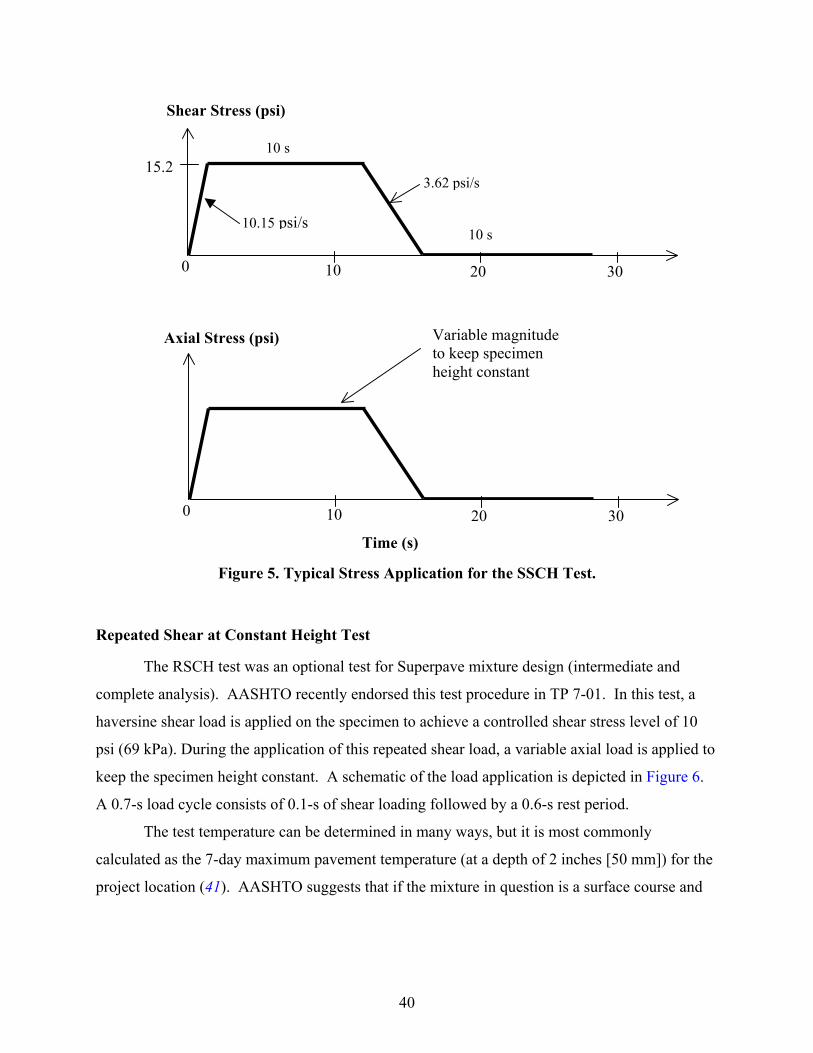
40
Figure 5. Typical Stress Application for the SSCH Test.
Repeated Shear at Constant Height Test
The RSCH test was an optional test for Superpave mixture design (intermediate and
complete analysis). AASHTO recently endorsed this test procedure in TP 7-01. In this test, a
haversine shear load is applied on the specimen to achieve a controlled shear stress level of 10
psi (69 kPa). During the application of this repeated shear load, a variable axial load is applied to
keep the specimen height constant. A schematic of the load application is depicted in Figure 6.
A 0.7-s load cycle consists of 0.1-s of shear loading followed by a 0.6-s rest period.
The test temperature can be determined in many ways, but it is most commonly
calculated as the 7-day maximum pavement temperature (at a depth of 2 inches [50 mm]) for the
project location (41). AASHTO suggests that if the mixture in question is a surface course and
Axial Stress (psi)
Time (s)
Shear Stress (psi)
0 30 10 20
Variable magnitude to keep specimen height constant
15.2
0 30 10 20
10 s
3.62 psi/s
10 s10.15 psi/s

41
Figure 6. Stress Pulses in the RSCH Test.
the thickness of the layer is less than 2 inches (50 mm), then actual layer thickness may be used
as the depth for calculating the test temperature. In this project, the project location is considered
to be College Station, Texas, and the surface mixture thickness is considered to be 2 inches (50
mm) or more. Pavement temperature at the project location was calculated using SHRP Manual
A-648A (42).
Using the SHRP A-648A manual, the 7-day maximum pavement temperature for College
Station, Texas, is found to be 140°F (60°C) with 50 percent reliability. Maximum pavement
temperature is calculated at depth of 0.8 inches (20 mm). Using the method presented in SHRP
Manual A-648-A, the temperature at a depth of 2 inches (50 mm) is calculated as 131°F (55°C)
for the design location. Researchers used the same test temperature for all four mixtures.
AASHTO suggests continued loading for 5000 load cycles or until the permanent shear
strain reaches 5 percent. Researchers decided to apply 10,000 load cycles or 5 percent strain,
0.7
Axial Stress (psi)
Time (s)
Shear Stress (psi)
0.1 1.4
0.1 0.7 1.4
Variable magnitude to keep specimen height constant
9.8

42
whichever comes first. The SST records the axial load, shear load, axial deformation, and shear
deformation. At the end of the test, the permanent shear strain is calculated and reported as a
percentage. Figure 7 illustrates a shearing deformation of a specimen subjected to repeated
loading. The strain curve has three distinct parts: large strain with few load applications due to
initial compaction, a linear pattern of steady rise in strain due to plastic deformation, followed by
an abrupt rise in strain after few more load applications. The latter part of the graph indicates
tertiary rutting, which usually occurs when the air void content falls below some critical value.
The presence of tertiary rutting also indicates that the mixture is very unstable or tender (9).
Figure 7. Permananent Deformation versus Repeated Load Applications.
Repeated Shear at Constant Stress Ratio Test
RSCSR is no longer included in the Superpave test protocols. This test was dropped
from the interim edition of AASHTO Provisional Standards in April 2001 (41). Before then, this
test was used for both intermediate and complete analysis of Superpave mixtures. This test was
considered as a screening test to delineate an asphalt mixture that is subject to tertiary rutting (4).
This form of rutting normally occurs at low air void contents and is a result of mixture
instability.
Log Number of Load Applications
Initial compaction
Tertiary Flow
Linear portion of permanent deformation
Log Permanent Strain

43
In the RSCSR test, repeated synchronized haversine shear and axial load pulses are
applied to the specimen as shown in Figure 8. The haversine ([1-cos 2]/2) load pulse
approximates the effect of a wheel load on a pavement (9). The load cycle requires 0.7 s,
wherein a 0.1-s load is followed by a 0.6-s rest period. The ratio of axial load to shear load is
maintained during the test at a constant ratio within the range of 1.2 to 1.5.
Figure 8. Stress Pulses in the RSCSR Test.
AASHTO suggests performing the test with 5000 cycles or 5 percent accumulated
shearing strain, whichever comes first. Based on previous experience, the researchers decided to
use 10,000 cycles or 5 percent accumulated shearing strain, whichever comes first because, with
only 5000 cycles of loading, most mixtures may not show any tertiary rutting. Researchers
decided to perform this test at same temperature (131°F [55°C]) as the RSCH test. The SST
records the axial load, shear load, axial deformation, and shear deformation. At the end of the
test, the permanent shear strain is calculated and reported in percent.
Axial Stress (psi)
Time (s)
Shear Stress (psi)
0.1 0.7 1.4
0.1 0.7 1.4
Variable magnitude to keep axial/shear stress between 1.2 and 1.5

44
ACCELERATED WHEEL TESTING
Researchers planned to conduct certain laboratory-scale rutting tests on the selected
HMA mixtures. The objectives of these tests were to compare the results from SST tests with
the results from laboratory-scale rut tests. Initially, researchers planned to conduct two
laboratory-scale tests: Asphalt Pavement Analyzer and 1/3-Scale Model Mobile Load Simulator.
Later, when two of the SST test protocols were dropped from the test plan due to AASHTO’s
recommendation, the Hamburg Wheel Tracking Device was included in the plan.
Asphalt Pavement Analyzer
The APA is a multifunctional loaded wheel tester used for evaluating permanent
deformation (Figure 9). Oscillating beveled aluminum wheels apply a repetitive load through
high-pressure hoses to generate the desired contact pressure. Rutting susceptibility of HMA can
be assessed by the APA using beam or cylindrical specimens under repetitive wheel loads and
measuring the amount of permanent deformation under the wheelpath.
In this study, six cylindrical specimens for each mixture were prepared using the
Superpave gyratory compactor. Specimen size was 6 inches (150 mm) in diameter and 3 inches
(75 mm) in height. The APA manufacturer recommends using three pairs of specimens to test
each mixture. Specimens were prepared with 4 percent air voids, and rutting tests were
performed at 147°F (64°C) for all the mixtures.
Each set of specimens was subjected to 8000 load cycles (31). One load cycle consists of
one forward and one backward movement of the wheel. The wheel load and hose pressure were
100 lb (445 N) and 100 psi (690 kPa), respectively. The vertical LVDT attached to the wheel
measures the rut depth at four different points on each set of specimens. Two specimens in one
mold form a set of specimens. Figure 10 shows the specimens set up in the APA machine. The
average of four readings is calculated as the rut depth of one set of specimens. The average of
three rut depths measured on three sets of specimens is reported as mixture rut depth.

45
Figure 9. Asphalt Pavement Analyzer.
Figure 10. APA Test Setup.
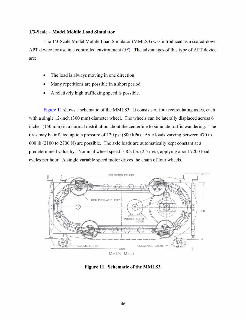
46
1/3-Scale – Model Mobile Load Simulator
The 1/3-Scale Model Mobile Load Simulator (MMLS3) was introduced as a scaled-down
APT device for use in a controlled environment (33). The advantages of this type of APT device
are:
• The load is always moving in one direction.
• Many repetitions are possible in a short period.
• A relatively high trafficking speed is possible.
Figure 11 shows a schematic of the MMLS3. It consists of four recirculating axles, each
with a single 12-inch (300 mm) diameter wheel. The wheels can be laterally displaced across 6
inches (150 mm) in a normal distribution about the centerline to simulate traffic wandering. The
tires may be inflated up to a pressure of 120 psi (800 kPa). Axle loads varying between 470 to
600 lb (2100 to 2700 N) are possible. The axle loads are automatically kept constant at a
predetermined value by. Nominal wheel speed is 8.2 ft/s (2.5 m/s), applying about 7200 load
cycles per hour. A single variable speed motor drives the chain of four wheels.
Figure 11. Schematic of the MMLS3.
47
MMLS-3 Test Specification
The following specifications were used for the MMLS3 tests described in this report:
Wheel load : 470 lb (2100 N)
Tire pressure : 100 psi (690 kPa)
Rate of loading : 6000 axles per hour
Test temperature : 122°F (50°C)
No lateral wandering of the wheel was applied during testing. MMLS3 testing
commenced after heating the compacted slabs for at least 12 hours. Stoppages during MMLS3
testing were limited to 25 minutes between profilometer measurements.
TxDOT MMLS3 Testing Facility
The materials laboratory at TxDOT in Austin was used for this test. Researchers
prepared the mixtures at TTI and hauled them to Austin for compaction and testing.
The MMLS3 tests were conducted in a temperature-controlled (environmental) chamber
specifically built for the device. The chamber allows testing to be performed at temperatures
ranging from 32 to 140°F (0 to 60°C). The chamber contains an overhead hoist for positioning
the MMLS3 and a laboratory compaction roller.
The compaction roller consists of guide rails, the mould, and a roller assembly. The
mould consists of two stackable metal frames with inside dimensions of 36 inches wide × 72
inches long (920 mm × 2800 mm). The bottom section has a thick metal floor. The mould fits
inside and is clamped to the guide rail assembly. The test pavement is constructed inside the
mould. The roller assembly contains an 18-inch diameter × 36-inch wide (450 mm diameter x
900 mm wide) steel drum. The drum is mounted onto a framework with four steel wheels that
run on the underside of the guide rails to provide a downward reaction force. The vertical
position of the drum is adjustable by means of a hand crank. A separate hand crank through a
chain and sprocket reduction system drives the drum.
The testing pad contained a semipermanent compacted HMA base, on which all four
were placed and compacted. The thickness of the existing base layer was about 3 inches.
Researchers raised the temperature of the environmental chamber to 50°C (122°F) and waited for
12 hours for temperature stabilization before starting the test.

48
Compaction of Test Pad
TTI prepared mixes for the MMLS3 tests in College Station and brought them to the
TxDOT materials laboratory in Austin (a 2-hour drive) in sealed drums placed within an
insulated “hotbox” for heat retention. The temperature loss of the mixtures in the drums was
typically on the order of 68°F (20°C). The sealed drums were immediately placed in a large
forced-draft oven, and the mixes were reheated to the appropriate compaction temperatures.
The same compaction procedure was adopted for each of the slabs. What follows is an
outline of this procedure. The surface of the existing base within the mould was covered with
roofing felt. The purpose of using the roofing felt was to protect the existing base layer during
removal of the surface layer after testing. After removal of the surface layer, no visual distress
was observed on the base layer. The roofing felt was painted with diluted emulsion tack coat on
top surface only. After the HMA material for the test slabs had reached compaction temperature,
it was placed within the MMLS3 test slab mould on top of the tacked roofing felt. A hoe and
shovels were used to spread the asphalt evenly within the mould. One pass with the compaction
roller was used to screed excess material and level the surface.
Breakdown compaction of the test slabs was performed manually using a gasoline-
powered vibratory plate compactor (tamper). Density of the slabs was monitored intermittently
during compaction using a nuclear density gauge that had been calibrated for each particular mix
prior to compaction. After the target density had been achieved using the plate compactor, 5 to
10 passes with the roller compactor were applied to smooth the pavement surface. A fine water
spray was used to prevent material from clinging to the drum. The final thickness of the
compacted layer was 70 mm.
In some cases, researchers placed a neoprene sheet between the drum and the pavement
surface to prevent transverse surface shear cracks during compaction when adequate density had
not been reached using the vibratory plate compactor.
MMLS3 Test Setup
Figure 12 shows a schematic of the MMLS test setup. The asphalt slabs were compacted
to a thickness of approximately 2.5 inches (62 mm) within the mould assembly. The MMLS3
was centered on top of the asphalt slab. The MMLS3 was not directly attached to the mould
assembly to prevent the transmission of vibrations and external forces onto the test slab. As will

49
be discussed later, the loading of the MMLS3 is uniform on a 3.28-ft (1 m) linear section
centered on the test slab. Test measurements were therefore confined to the shaded test area
indicated in Figure 12, although the MMLS tire track extends beyond this area.
Transverse profilometer measurements were taken at three locations centered 10 inches
(250 mm) apart along the test area, as shown on Figure 12. These transverse profiles were
designated A, B, and C in the direction of travel.
Figure 12. Schematic of MMLS3 Test Setup.
Figure 12 indicates the relative positions of thermocouples installed in the slab as well as
possible positions of cores within and outside of the wheel track that were taken for density
measurements after MMLS3 testing. The wheel track without application of the wandering
function is about 3.15 inches (80 mm) wide.
Temperature Control
Each of the MMLS tests was performed within a temperature-controlled environmental
chamber with the asphalt slabs heated to 122°F (50°C).
72 in
36 in
10 in 10 in
40 in
Mould assembly
MMLS profile
A B C
Direction of travel
Test area
MMLS track
Transverse profiles Thermocouples
Cores

50
Researchers installed four bead probe K-type thermocouples within the asphalt slab to
monitor temperature during the tests, two on the surface, one at a depth of 1 inch (25 mm), and
another at a depth of 2 inches (50 mm) beneath the surface of the asphalt. These were glued to
the slab surface using quick-drying epoxy. The temperature of the asphalt slab was monitored on
a regular basis with adjustments made, if necessary.
Typically, the asphalt slabs required about 5 hours of heating before the temperature
stabilized to 122°F. After initial profilometer measurements, if necessary, MMLS3 trafficking
was delayed shortly to allow the pavement surface temperature to return to 122°F.
It should be noted that heating of the environmental chamber alone allowed the full depth
of the asphalt slab to be heated to 122°F. The use of the surface plenum ducts was not necessary.
Profilometer Measurements and Rutting Definition
The profilometer rutting measurement system consists of a 3.28-ft (1 m) long sliding
plate frame to which a vertical reader unit is attached. The frame fits into two aluminum
extrusion tracks (guide rails) that are mounted on both sides of the mould configuration and that
serve as the reference datum for the vertical rut measurements. The vertical reader is attached to
a Mitutoyo KM/KC counter display unit, which in turn is connected to a laptop computer via the
RS-232 port.
The vertical reader is free to move horizontally and incorporates an arm, which is free to
move vertically, connected to a 2-inch (50 mm) diameter wheel that travels along the surface
profile being measured. This allows profilometer measurements to be captured as a two-
dimensional array (x, y) on the computer.
During an MMLS3 test, profilometer measurements were taken prior to MMLS3
trafficking and thereafter at specific intervals during trafficking to allow an accurate definition of
the cumulative rutting curve. Since the maximum number of axles to be applied for this test
series was limited to 100,000 per test, researchers decided to take readings after the following
number of axles: 0, 1,000, 10,000, 50,000, and 100,000. Three transverse profilometer
measurements were taken after each interval at locations described previously and indicated in
Figure 12.
Rutting profiles or surface elevations with trafficking are developed relative to the
transverse profiles taken before MMLS3 trafficking (i.e., 0-axles reading). The maximum rut

51
depths given in this report were determined by applying an imaginary straight edge over the
maximum surface elevations and calculating the vertical distance to the lowest surface elevation,
as shown in Figure 13.
Figure 13. Adjustments to Vertical Transverse Surface Profiles.
When necessary, researchers made minor adjustments to the rutting profiles to account
for errors resulting from temperature effects and misalignment. The profilometer measures a
transverse surface profile across a total width of about 25 inches (750 mm). The rutting profile is
centered across 4 to 5 inches (80 to 100 mm) on this total profile. Shoving is usually apparent at
the edges of the rut extending about 6-8 inches (150-200 mm), as shown in Figure 13. The
profile beyond the shoving range is not influenced by loading and may be used as a reference for
adjusting vertical deviations. The difference in the sum of squares of two load-free profiles is
minimized to adjust vertical profiles.
The profilometer (Figure 14) used for the rutting measurements is accurate to 0.008
inches (0.2 mm) in the horizontal and vertical directions.
Vertical adjustment
Rut width
Total transverse profile
Shoving
Load-free profile
Original profile 2
Adjusted profile 2
Imaginary straight edge
Maximum rut Profile 1

52
Figure 14. Profilometer Used to Measure MMLS3 Rut Depth.
Hamburg Wheel Tracking Device
Unlike the other laboratory-scale rut testers, the HWTD test is always conducted in
submerged condition. Besides many other properties, this device provides the moisture
susceptibility information of the HMA mixture. Researchers tested all four mixtures using two
different HWTDs following TxDOT specification Tex-242-F.
Researchers conducted HWTD tests at the TxDOT laboratory at Austin (Figure 15).
Accordingly, specimens for each mixture were compacted and saw cut at the TTI laboratory and
tested at the TxDOT facility. These HWTD tests were repeated near the end of the project at the
TTI laboratory when the new TTI machine was installed. Precision Metal Works (PMW),
Salina, Kansas, manufactured both machines.
Four specimens of each of the four mixtures were compacted using the Superpave
gyratory compactor. Cylindrical specimens were compacted following the AASHTO TP4
standard. The specimens are 6 inches (150 mm) in diameter and 2.5 inches (63 mm) high. One
cylindrical side of each specimen was trimmed slightly so that two specimens together form a set
and fit into the mold (Figure 15). The sample setup is shown in Figure 16. The measured air
void content of each specimen was within 7 ± 1 percent. A circulating water pump and a water
heater keeps the water temperature constant at 122 ± 2°F (50 ± 1°C) throughout the test. The
HWTD is programmed to start 30 minutes after the water temperature reaches the desired level.
This 30-minute time period is designed to precondition the submerged specimens. The machine

53
Figure 15. Hamburg Wheel Tracking Device Mold.
Figure 16. HWTD Loaded with Specimens.
Thickness = 2.45 inch“Acrylic” Sheet
1.6 inch 1.6 inch 6 inch
6 inch
0.3 inch 0.3 inch
14.5 inch

54
was set to terminate the test at 20,000 cycles or 0.5 inches (12.5 mm) of rut depth, whichever
occurs first. It is noteworthy that one forward and one backward pass of wheel comprise two
cycles. All the tests were conducted at the rate of 52 cycles/minute.
Table 9 summarizes the test conditions and specimen description for all mixtures.
Table 9. Test Condition and Specimen Description for the Different Mixtures.
Mixture Type Test Identification
Asphalt Content
Number of Specimens
Tested
Air Voids (%)
Test Temperature (°F)
Limestone Type-C
FSCH SSCH RSCH RSCSR APA Hamburg MMLS-3
Design Design Design Design Design Design Design
3 3 3 3 6 4 One Slab*
7 7 3 3 4 7 7
39, 68, and 104 39, 68, and 104 131 131 147 122 122
River Gravel
FSCH SSCH RSCH RSCSR APA Hamburg MMLS-3
Design Design Design Design Design Design Design
3 3 3 3 6 4 One Slab*
7 7 3 3 4 7 7
39, 68, and 104 39, 68, and 104 131 131 147 122 122
Granite SMA
FSCH SSCH RSCH RSCSR APA Hamburg MMLS-3
Design Design Design Design Design Design Design
3 3 3 3 6 4 One Slab*
7 7 3 3 4 7 7
39, 68, and 104 39, 68, and 104 131 131 147 122 122
Granite Superpave
FSCH SSCH RSCH RSCSR APA Hamburg MMLS-3
Design Design Design Design Design Design Design
3 3 3 3 6 4 One Slab*
7 7 3 3 4 7 7
39, 68, and 104 39, 68, and 104 131 131 147 122 122
* Readings were taken at three different locations

55
CHAPTER 4: RESULTS AND DISCUSSIONS
GENERAL
Researchers tested four different asphalt mixtures using four different types of SST
testing and three different types of accelerated loading wheel tests to evaluate their permanent
deformation resistance characteristics.
While conducting the tests, researchers were careful to follow the appropriate test
standards. Although tests were performed in different time periods of the project, researchers
always tested freshly made specimens to avoid the effects of aging. The results of each test are
described separately.
SUPERPAVE SHEAR TESTER
The four selected HMA mixtures were tested using the SST machine following four
different test protocols. Details of the test procedures are presented in Chapter 3. The following
paragraphs describe the SST results.
Frequency Sweep at Constant Height
Researchers conducted the FSCH test at three different temperatures and on three
specimens from each mixture. Specimens were tested at the lower temperature and then at the
higher temperature to minimize the damage caused by shearing strain. The frequency sweep test
was performed using 10 different frequencies, starting at the higher frequency toward the lower.
The test applies a repeated sinusoidal horizontal shear strain with peak amplitude of
approximately ±0.005 percent and a variable axial stress to maintain constant specimen height.
Shear strain is applied at different frequencies, including 10, 5, 2, 1, 0.5, 0.2, 0.1, 0.05, 0.02, and
0.01 Hz. The specified strain level was selected during the SHRP program to ensure that the
viscoelastic response of the asphalt mixture is within the linear range. This means that the ratio
of stress to strain is a function of loading time and not of the stress magnitude. In some cases
within this range of frequencies, it has been observed that at the high and low frequencies the
behavior becomes nonlinear. Huber (42) shows that the dynamic shear modulus (ratio of stress
to strain) of asphalt cement is approximately linear between the frequency range of 0.01 to 10
Hz.

56
Before testing, the specimens were preconditioned by applying a controlled sinusoidal
shear strain at a frequency of 10 Hz for 100 cycles and peak-to-peak amplitude of 0.0001
mm/mm. A detailed description of this test method is given in AASHTO TP7, Procedure A (41)
and Superpave Asphalt Mixture Analysis: Lab Notes (43).
Axial deformation, shear deformation, axial load, shear load, and temperature at each of
the 10 different frequencies were recorded. The data obtained from the FSCH test were used to
calculate two properties: complex shear modulus (with its real and imaginary parts) and phase
angle.
Complex Shear Modulus
Raw data recorded from SST machine were fed into ATS software to calculate the
complex shear modulus (CSM) and shear phase angle (SPA) for each frequency. Figures 17, 18,
and 19 show the mean complex shear modulus of all mixtures plotted against the logarithm of
frequency and tested at 39, 68, and 104°F, respectively.
Figure 17. Complex Shear Modulus at 39°F.
Figure 17 illustrates that CSM increases linearly with the increasing frequency. The
CSMs for the limestone and SMA mixtures remained very close throughout the frequency range.
The river gravel mixture consistently yielded the lowest CSM. At this low temperature (39°F),
0.0E+00
1.0E+09
2.0E+09
3.0E+09
4.0E+09
0.01 0.1 1 10
Frequency (Hz)
Com
plex
She
ar M
odul
us (p
si) Avg CSM for LS
Avg CSM for RG Avg CSM for SMAAvg CSM for SUP

57
the difference between the CSMs for the different mixtures appears the same, regardless of
frequency.
Figure 18. Complex Shear Modulus at 68°F.
Figure 19. Complex Shear Modulus at 104°F.
In Figure 18, the CSM values increase significantly with frequency. The complex shear
moduli of all mixtures are similar at lower frequencies, and they diverge exponentially at higher
frequencies. The granite SMA mixture shows the highest CSM for all frequency ranges,
followed by limestone mixture. In Figure 19, the granite SMA mixture shows a marginally
0.0E+00
5.0E+08
1.0E+09
1.5E+09
2.0E+09
0.01 0.1 1 10Frequency (Hz)
Com
plex
She
ar M
odul
us (p
si) Avg CSM for LS
Avg CSM for RGAvg CSM for SMAAvg CSM for SUP
0.0E+00
2.0E+08
4.0E+08
6.0E+08
8.0E+08
1.0E+09
0.01 0.1 1 10
Frequency (Hz)
Com
plex
She
ar M
odul
us (p
si) Avg CSM for LS
Avg CSM for RGAvg CSM for SMAAvg CSM for SUP

58
higher CSM than limestone mixture at frequencies above 1 Hz. The position of granite
Superpave and river gravel mixtures are distinct in both Figures 18 and 19.
Shear Phase Angle
Shear phase angle is defined as the lag time between the application of a stress and the
corresponding strain. SPA was calculated using the ATS software (44). Figures 20, 21, and 22
Figure 20. Shear Phase Angle versus Frequency at 39°F.
Figure 21. Shear Phase Angle versus Frequency at 68°F.
0
5
10
15
20
25
30
0.01 0.1 1 10
Frequency (Hz)
Shea
r Pha
se A
ngle
(deg
ree)
Avg SPA for LSAvg SPA for RGAvg SPA for SMAAvg SPA for SUP
25
30
35
40
45
0.01 0.1 1 10
Frequency (Hz)
Shea
r Pha
se A
ngle
(deg
ree)
Avg SPA for LSAvg SPA for RGAvg SPA for SMA Avg SPA for SUP

59
present the mean SPA from tests at 39, 68, and 104°F, respectively. At 39°F, the SPA of each
mixture follows a similar trend. In Figure 20, the limestone and granite SMA mixtures show
lowest SPA. River gravel always yields highest SPA, and granite Superpave is near the center of
the plots.
Figure 22. Shear Phase Angle versus Frequency at 104°F.
In Figures 21 and 22, the trends are not consistent but the river gravel mixture generally
exhibits the highest angle, while the limestone and granite SMA yield the lower range of SPA.
Sometimes, the G*/sin δ term is used to estimate the rutting susceptibility of HMA
mixtures. Since SPA (δ) was not very consistent, researchers did not pursue plotting G*/sin δ.
Simple Shear at Constant Height
The SSCH test was performed at three different stress levels and test temperatures (Table
10). Shear stress was applied at a rate of 10.15 ± 0.72 psi (70 ± 5 kPa) per s up to the stress level
indicated in Table 10. The stress level was maintained for 10 s and then reduced to zero at a rate
of 3.62 psi/s (25 kPa/s). As the specimen is sheared, it tries to dilate (increase in height). A
variable (controlled by axial LVDT feedback) axial load was applied to maintain a constant
specimen height (±0.0005 inch).
All specimens were preconditioned for 100 cycles with a shear stress having a peak
magnitude of approximately 1.0 psi (6.9 kPa). Each cycle has duration of 0.7 s, consisting of a
0.1-s loading period followed by a 0.6-s rest period in a haversine wave form.
35
40
45
50
55
60
65
0.01 0.1 1 10
Frequency (Hz)
Shea
r Pha
se A
ngle
(deg
ree)
Avg SPA for LS Avg SPA for RG Avg SPA for SMA Avg SPA for SUP

60
Table 10. Stress Level Applied in the SSCH Test.
Test Temperature, °F (°C) Shear Stress, psi (kPa) 39 (4) 50 (345)
68 (20) 15.2 (105) 104 (40) 5.1 (35)
The SSCH was performed after the FSCH test using the same specimens. The tests at the
lowest temperatures were performed first. A detailed description of this test method is provided
in AASHTO TP7, Procedure B (41) and Superpave Asphalt Mixture Analysis: Lab Notes (43).
Researchers recorded the axial deformation, shear deformation, axial load, shear load,
and temperature throughout the test. Material properties calculated from the recorded data were
maximum shear strain, permanent shear strain, and elastic recovery. Data were manually
analyzed using a spreadsheet.
Maximum Shear Strain
Maximum shear strain usually occurs at the end of a steady applied load before it starts
decreasing. This strain measurement indicates the total deformation susceptibility of the
mixture. It is calculated using the following formula:
hinitialshear,maximumshear,
max
δδγ
−= ,
where: (max = maximum shear strain,
*shear, maximum = maximum deformation recorded by the LVDT,
*shear, initial = initial shear deformation at the start of the test, and
h = gauge length, 1.5 inches (38 mm).
Permanent Shear Strain
Permanent shear strain is the deformation measured at the end of the test. It indicates the
plastic deformation characteristics of the mixture. Permanent shear strain is calculated by
subtracting the initial shear deformation from the final shear deformation and dividing that
number by the gauge length of shear LVDT. SSCH test results are shown in Table 11.

61
Table 11. SSCH Test Result.
Test Temperature, °F (°C) Measured Property 39 (4) 68 (20) 104 (40) Limestone Mixture
Maximum Strain (in/in) 0.00025267 0.00106227 0.00067080 Permanent Strain (in/in) 0.00004533 0.00052080 0.00036080 Elastic Recovery (%) 82.31 50.55 46.07
River Gravel Mixture Maximum Strain (in/in) 0.00068613 0.00248120 0.00403800 Permanent Strain (in/in) 0.00026560 0.00146107 0.00279660 Elastic Recovery (%) 62.40 41.16 30.40
Granite SMA Maximum Strain (in/in) 0.00023040 0.00066187 0.00104267 Permanent Strain (in/in) 0.00004360 0.00035933 0.00062200 Elastic Recovery (%) 81.32 51.87 40.73
Granite Superpave Maximum Strain (in/in) 0.00041227 0.00160720 0.00153347 Permanent Strain (in/in) 0.00013133 0.00102280 0.00097600 Elastic Recovery (%) 68.91 38.20 36.57
Elastic Recovery
When the load imposed on the specimen is withdrawn, the specimen partially rebounds to
its original shape. This phenomenon is due to the elastic properties of the mixture. More elastic
recovery indicates better resistance to permanent deformation. Elastic recovery is calculated
using the following equation.
100Recoveryfinalshear,
finalshear,maximumshear, ×−
=δ
δδ,
Where: Recovery = percentage of shear deformation recovered after the removal of
load,
*shear,maximum = maximum recorded deformation by the shear LVDT, and
*shear,final = final recorded shear deformation at the end of the test.

62
Figures 23, 24, and 25 present the maximum shear strain, permanent shear strain, and
elastic recovery, respectively. In these figures, the mixture designation is abbreviated. For
example, SM104 means granite SMA mixture tested at 104°F. Clearly, the river gravel mixture
demonstrates the highest maximum shear strain and permanent shear strain at all temperatures.
Figure 23. Maximum Shear Strain for Different Mixtures.
Figure 24. Permanenet Shear Strain for Different Mixtures.
0.000
0.001
0.002
0.003
0.004
0.005
LS03
9
LS06
8
LS10
4
SM03
9
SM06
8
SM10
4
RG
039
RG
068
RG
104
SP03
9
SP06
8
SP10
4
Mixture Type
Max
imiu
m S
trai
n (in
/in)
0.000
0.001
0.001
0.002
0.002
0.003
0.003
LS03
9
LS06
8
LS10
4
SM03
9
SM06
8
SM10
4
RG
039
RG
068
RG
104
SP03
9
SP06
8
SP10
4
Mixture Type
Perm
anen
t Str
ain
(in/in
)

63
Elastic recoveries at the lower test temperature are higher than those at the higher temperature
for every mixture. Elastic recovery for the different mixtures tested at the same temperature does
not vary appreciably.
Considering results at the same temperature, the limestone mixture and granite SMA
mixture are very similar with respect to the three properties measured by SSCH test. The granite
Superpave mixture yielded higher maximum strain and permanent strain than the limestone and
granite SMA mixtures.
Figure 25. Elastic Recovery of Different Mixtures.
Repeated Shear at Constant Height
In the RSCH test, repeated haversine shear load pulses (10 psi [69 kPa]) were applied to
the specimen. When the shear load is applied, the test specimen tends to dilate. To prevent
vertical dilation, a controlled axial load is applied to keep the specimen at a constant height. The
loading cycle requires 0.7 s, wherein a 0.1-s load is followed by 0.6-s rest period. This test was
performed at the design asphalt content. Specimens containing 3 percent air voids were used to
increase their sensitivity to tertiary rutting. Air voids of 3 percent were achieved by applying
more gyrations during the compaction process.
Before testing, the specimens were preconditioned by applying 100 cycles of a haversine
shear load with a peak magnitude of 1 psi (6.9 kPa). After preconditioning, the specimens were
0
20
40
60
80
100
LS03
9
LS06
8
LS10
4
SM
039
SM
068
SM
104
RG
039
RG
068
RG
104
SP
039
SP
068
SP
104
Mixture Type
Elas
tic R
ecov
ery
(%)

64
subjected to 10,000 load cycles at a temperature of 131°F (55°C) in accordance with the ATS
Manual, Version 3.1 (44) and AASHTO TP7, Procedure C (41). Chapter 3 describes
determination of test temperature.
The permanent shearing strain after 10,000 cycles of each specimen and their average is
depicted in Figure 26. Permanent shearing strain was calculated from the recorded data using the
following equation.
hγ initialshear,finalshear,
p
δδ −= ,
where, (p = permanent shear strain,
*shear,final = final deformation recorded by the shear LVDT at the end of
the test (10,000 cycles),
*shear,initial = initial deformation at the start of the test (nominally zero), and
h = the gauge length of shear LVDT, 1.5 inch (38 mm).
Figure 26. Permanent Shear Strain from RSCH Test.
The river gravel mixture experienced substantial accumulated shear strain. The test was
set up for 10,000 cycles or 5 percent accumulated strain, whichever comes first. Except for the
river gravel mixture, each specimen from all other mixtures completed 10,000 load cycles. River
gravel specimens survived only about 2000 cycles before failure. The bar chart (Figure 26)
0
1
2
3
4
5
Limestone River Gravel Granite SMA Granite SpMixture Type
Perm
anen
t Str
ain
(%)
Spec 1 Spec 2 Spec 3 Average
River Gravel Specimens Tested at about 2000 cycles

65
shows that the limestone mixture yielded lowest strain. The granite SMA yielded higher strains
than limestone, and granite Superpave yielded higher strains than granite SMA.
Repeated Shear at Constant Stress Ratio
The shear stress and axial stress selected correspond to a strong base condition and was
14.2 psi (98 kPa) and 21.45 psi (148 kPa), respectively (9, 43). This test was performed at the
design asphalt content, but at 3 percent air voids to enhance tertiary rutting
All specimens were preconditioned by applying 100 cycles of shear load pulses with a
peak magnitude of 1 psi (6.9 kPa) and corresponding axial loads. After preconditioning the
specimens, the repeated shear test was initiated. A detailed description of this test method is
given in AASHTO TP7, Procedure C (5). The test was conducted at 131°F (55°C) and was set
to apply a maximum of 10,000 load cycles or 5 percent accumulated permanent shear strain,
which ever comes first. Permanent shear strain was calculated using the following equation.
hinitialshear,finalshear,
p
δδγ
−= ,
where, (p = permanent shear strain,
*shear,final = final deformation recorded by the shear LVDT at the end of
the test (10,000 cycles),
*shear,initial = initial deformation at the start of the test (nominally zero), and
h = gauge length of shear LVDT, 1.5 inch (38 mm).
Figure 27 depicts the accumulated permanent shear strain at the end of the test. Like the
RSCH test, the river gravel mixture did not survive 10,000 load cycles. The specimens failed
between 1200 and 2200 cycles. In this test, the granite SMA mixture yielded the lowest
permanent strain. The limestone mixture yielded marginally higher strain than the granite
Superpave mixture.

66
Figure 27. Permanent Shear Strain from RSCSR Test.
Mixture Rankings by SST Protocols
All SST test results were used to rank the mixtures regarding their resistance to
permanent deformation. The FSCH test provides two material properties: complex shear
modulus and shear phase angle. Higher complex modulus indicates higher rut resistance. Lower
phase angle indicates more elastic behavior of the mixture and thus higher rut resistance. On the
basis of the CSM and SPA values, researchers ranked the mixtures. A ranking of 1 means
highest rut resistance and higher numbers indicate higher rut susceptibility. Sometimes, the
values were so close that the same rank was given to more than one mixture. Table 12 exhibits
the mixture rankings prepared from the FSCH test results. CSM and SPA were determined for
each of the
Table 12. Mixture Rankings by FSCH Test.
Test at 39°F Test at 68°F Test at 104°F Mixture Type G* at
10 Hz Overall1
δ Overall1
G* G* at 10 Hz
Overall1 δ
Overall1 G*
G* at 10 Hz
Overall1 δ
Overall1
G* Limestone 1 1 1 2 1 2 2 1
River Gravel 4 4 4 4 4 4 4 4 4
Granite SMA 2 1 1 1 1 1 1 2 1
Granite Superpave 3 3 3 3 3 3 3 2 3 1 Overall ranking was derived from the position of the plot.
0
1
2
3
4
5
Limestone River Gravel Granite SMA Granite Sp
Mixture Type
Perm
anen
et S
trai
n (%
)
Spec 1 Spec 2 Spec 3 Average
River Gravel Specimens Tested to only 1200 - 2000 cycles

67
10 frequencies and at three different temperatures. The CSMs were used in two ways to
determine the rankings: CSM at 10 Hz and the CSM versus frequency graphs. The reason for
using CSM at 10 Hz was that this frequency resembles that of highway traffic. Since the shear
phase angle did not follow a consistent trend, the overall SPA (SPA versus frequency graph) was
used for ranking.
Rankings of the river gravel mixture were very consistent, as shown in Table 12. The
granite SMA appears to be the most rut resistant mixture, followed by the limestone and granite
Superpave mixtures. Generally, the rankings from the FSCH test were quite consistent.
Table 13 provides mixture rankings prepared from the SSCH test results. Three material
responses used in this ranking are: maximum shear strain (MS), permanent shear strain (PS), and
elastic recovery (ER). Higher maximum shear strain and higher permanent shear strain both
indicate of more rut susceptibility. On the other hand, higher elastic recovery indicates lower rut
susceptibility. Ranking for SSCH at 39 and 68°F were quite consistent but changed a little at
104°F.
Table 13. Mixture Rankings by SSCH Test.
Test at 39°F Test at 68°F Test at 104°F Mixture Type MS PS ER MS PS ER MS PS ER
Limestone 2 2 1 2 2 1 1 1 1 River Gravel 4 4 4 4 4 2 4 4 2 Granite SMA 1 1 2 1 1 1 2 2 2 Granite Superpave 3 3 3 3 3 4 3 3 4
MS - Maximum Strain PS - Permanent Strain ER - Elastic Recovery
Table 14 presents mixture rankings from RSCH and RSCSR test results. In both tests,
accumulated permanent shearing strain at the end of the test was used to rank the mixtures. The
limestone mixture performed best in the RSCH test, and granite SMA performed best in the
RSCSR test. Performance of the limestone and granite Superpave mixtures in the RSCSR test
was very similar. The performances of the river gravel mixture in both tests were the worst, as
expected.

68
Table 14. Mixture Rankings by Repeated Shear Tests.
Ranking Type of Mixture
RSCH RSCSR
Limestone 1 2 River Gravel 4 4 Granite SMA 2 1 Granite Superpave 3 2
RESULTS FROM LOADED WHEEL TESTERS
Researchers conducted three different types of laboratory-scale accelerated loaded wheel
tests on the four mixtures studied. The purpose of this testing was to compare the results with
those from the SST. Although the wheel testers do not provide basic material properties, they
have the ability to rank rutting susceptibility of HMA mixtures, as indicated in literature (19, 20,
25).
Asphalt Pavement Analyzer
The final rut depths measured by the APA for the four mixtures are given in Table 15 and
Figure 28. Only the river gravel mixture could not withstand the complete 8000 cycles. The
average rut depth experienced by the river gravel mixture was 0.71 inches at 6000 cycles. The
test was stopped at that point because at that level of rutting, the wheel can no longer apply a full
load due to excessive sagging of the pressure hose.
Table 15. Final Rut Depth Measured by APA.
Rut Depth at 8000 Cycles (inch) Mixture Type
Left Set Middle Set Right Set
Average Rut Depth
(inch) Limestone 0.211 0.188 0.174 0.191 River Gravel * 0.783 0.673 0.666 0.707 Granite SMA 0.136 0.113 0.105 0.118 Granite Superpave 0.150 0.150 0.179 0.159
*at about 6000 cycles

69
The granite SMA mixture performed the best in the APA test, followed by granite
Superpave and limestone mixtures. Figure 29 exhibits the mean cumulative rut depth of all
mixtures.
Figure 28. Rut Depth Measured by APA.
Figure 29. Comparison of Mean Cummulative Rutting (APA).
0.00
0.10
0.20
0.30
0.40
0.50
0.60
0.70
0.80
0 2,000 4,000 6,000 8,000 10,000
Number of Cycles
Rut
Dep
th (i
nch) Limestone
River GravelGranite SMAGranite Superpave
0.0
0.2
0.4
0.6
0.8
1.0
Limestone River Gravel Granite SMA Granite Sp
Mixture Type
Rut
Dep
th (i
nch)
Left Middle Right Average

70
Model Mobile Load Simulator – 1/3 Scale
Unlike the other loaded wheel testers, researchers measured rut depth from the MMLS3
manually. Details of the MMLS3 are presented in Chapter 3. Bulging of the HMA above the
surface datum alongside the wheelpath is clearly apparent in the rutting profiles measured for
each of the MMLS3 tests. The degree of bulging varies from about 0.02 inches (0.5 mm) for the
granite SMA mixture to about 0.2 inches (5 mm) for the river gravel mixture. This indicates that
some of the deformation occurred without a change in volume.
Figure 30 shows details of a MMLS3 rut measurement from the granite SMA. The rise or
peak within the wheelpath is about 0.2 inches (0.5 mm) high and is the outline of an aggregate
particle jutting out. It can be seen that initially (and even after 1000 axle loads), this particle
was embedded but with additional trafficking, the mortar and material alongside the particle was
displaced. Definition of maximum rut depth is clearly influenced by this irregular rut profile.
For the purpose of this report, maximum rut depths were measured to the deepest trough within
the rut path.
The intent was to terminate MMLS3 trafficking after the application of 100,000 axles or
whenever a mix developed a 0.4 inches (0.10 mm) rut, whichever occurred first. Tests on the
river gravel mixture were terminated prematurely due to excessive rutting, and 120,000 axles
were applied to the granite SMA mixture, the test overrunning slightly.
Figure 30. Zoom of a Typical MMLS3 Wheelpath Rut Measurement.

71
Limestone
Figure 31 shows cumulative rutting measured across the three transverse positions for the
limestone mixture. Mean rut depth after the application of 100,000 MMLS3 axles was about
0.25 inches (6.4 mm). Deviation of the rutting across the three transverse positions increased
with trafficking. Most of the rutting occurred in first 10,000 axles.
Figure 31. Cumulative Rutting on Limestone Mixture.
River Gravel
Figure 32 shows cumulative rutting measured across the three transverse test positions for
the river gravel mixture. This test ended prematurely, with the material rutting in excess of 0.6
inches (15 mm) after only 5000 MMLS3 load applications. Anticipating the premature failure of
this tender mixture, researchers recorded a set of readings at 100 axles.
0
0.1
0.2
0.3
0.4
0 20 40 60 80 100
MMLS3 Axles (Thousand)
Cum
ulat
ive
Rut
Dep
th (i
nch)
Set 1Set 2Set 3
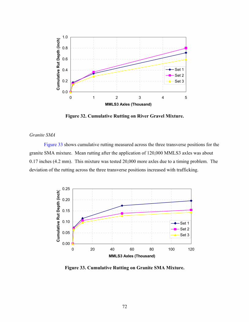
72
Figure 32. Cumulative Rutting on River Gravel Mixture.
Granite SMA
Figure 33 shows cumulative rutting measured across the three transverse positions for the
granite SMA mixture. Mean rutting after the application of 120,000 MMLS3 axles was about
0.17 inches (4.2 mm). This mixture was tested 20,000 more axles due to a timing problem. The
deviation of the rutting across the three transverse positions increased with trafficking.
Figure 33. Cumulative Rutting on Granite SMA Mixture.
0.0
0.2
0.4
0.6
0.8
1.0
0 1 2 3 4 5
MMLS3 Axles (Thousand)
Cum
ulat
ive
Rut
Dep
th (i
nch)
Set 1Set 2Set 3
0.00
0.05
0.10
0.15
0.20
0.25
0 20 40 60 80 100 120
MMLS3 Axles (Thousand)
Cum
ulat
ive
Rut
Dep
th (i
nch)
Set 1Set 2Set 3

73
Granite Superpave
Figure 34 shows cumulative rutting measured across the three transverse positions for the
granite Superpave mixture. Mean rutting after the application of 100,000 MMLS3 axles was on
the order of 0.32 inches (8.1 mm). Like the other mixtures, the deviation for the rutting across
the three transverse positions increased with trafficking.
Figure 35 compares the mean cumulative rutting for the four mixtures tested. In each of
the tests, the rutting developed quickly, with more than 0.1 inches (2.5 mm) of rutting within the
first 10,000 load applications. Based on Figure 34, the mixtures rank from best to worst as
granite SMA, limestone, granite Superpave, and river gravel mixture.
Figure 34. Cumulative Rutting on Granite Superpave Mixture.
Slab Density
The intention was to compact each of the slabs for the MMLS tests to the same density
(93 percent of theoretical maximum density). But in practice, this was not possible due to the
small size of the test slab and the compaction equipment available. Slab densities were
monitored during compaction using a nuclear density gauge. After completion of MMLS rut
testing, sections of each slab were removed and cores were cut from these sections (inside and
outside of the trafficked wheel paths) to verify actual slab compaction and to evaluate the change
in density (in the MMLS wheelpaths) with trafficking. The results are shown in Table 16.
0.0
0.1
0.2
0.3
0.4
0 20 40 60 80 100
MMLS3 Axles (Thousands)
Cum
ulat
ive
Rut
Dep
th (i
nch)
Set 1Set 2Set 3

74
Figure 35. Comparison of Mean Cumulative Rutting for All Mixtures (MMLS3).
Table 16. MMLS3 Slab Density.
Voids in the Mix Outside Wheelpath Inside Wheelpath Mixture Type 1 2 Avg. 1 2 Avg.
Limestone 8.11 7.50 7.81 5.64 5.11 5.38 River gravel* 3.55 3.68 3.62 2.85 2.89 2.87 Granite SMA 6.0 6.1 6.05 6.1 6.0 6.05 Granite Superpave 6.05 5.93 5.99 4.03 4.55 4.29
* Tested to only 5000 MMLS3 axles
There were significant differences in the initial compaction densities of the slabs before
MMLS3 testing (Table 16). Air voids in the granite (SMA and Superpave) and limestone mixes
were reasonably similar (7 ± 1 percent) but the river gravel mixture was over compacted. It is
noteworthy that no change in the density of the SMA mix was apparent with trafficking. This is
because the SMA design yields stone to stone contact of the angular coarse aggregate.
Hamburg Wheel Tracking Device
Due to late delivery of TTI-owned HWTD, researchers performed the test at the TxDOT
laboratory in Austin. Accordingly, specimens for each mixture were compacted and saw cut at
0
0.1
0.2
0.3
0.4
0.5
0.6
0 20 40 60 80 100 120 140MMLS3 Axles (Thousand)
Cum
mul
ativ
e R
ut D
epth
(inc
h)
LimestoneRiver GravelGranite SMAGranite Superpave
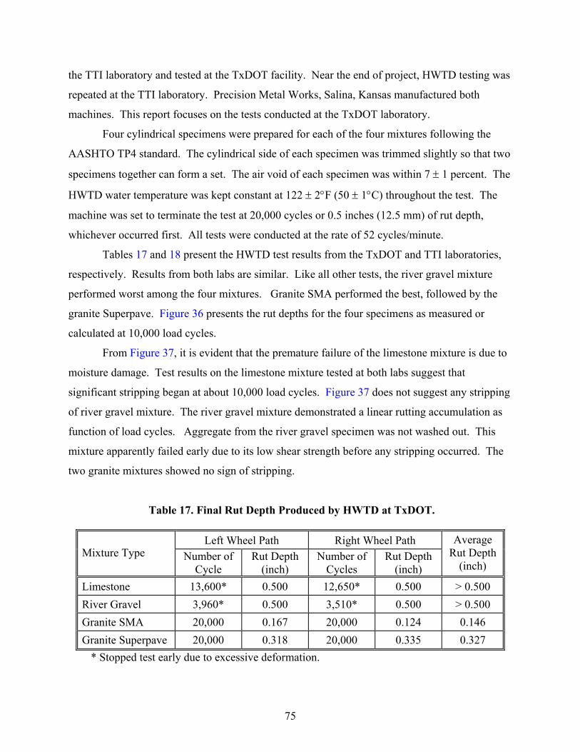
75
the TTI laboratory and tested at the TxDOT facility. Near the end of project, HWTD testing was
repeated at the TTI laboratory. Precision Metal Works, Salina, Kansas manufactured both
machines. This report focuses on the tests conducted at the TxDOT laboratory.
Four cylindrical specimens were prepared for each of the four mixtures following the
AASHTO TP4 standard. The cylindrical side of each specimen was trimmed slightly so that two
specimens together can form a set. The air void of each specimen was within 7 ± 1 percent. The
HWTD water temperature was kept constant at 122 ± 2°F (50 ± 1°C) throughout the test. The
machine was set to terminate the test at 20,000 cycles or 0.5 inches (12.5 mm) of rut depth,
whichever occurred first. All tests were conducted at the rate of 52 cycles/minute.
Tables 17 and 18 present the HWTD test results from the TxDOT and TTI laboratories,
respectively. Results from both labs are similar. Like all other tests, the river gravel mixture
performed worst among the four mixtures. Granite SMA performed the best, followed by the
granite Superpave. Figure 36 presents the rut depths for the four specimens as measured or
calculated at 10,000 load cycles.
From Figure 37, it is evident that the premature failure of the limestone mixture is due to
moisture damage. Test results on the limestone mixture tested at both labs suggest that
significant stripping began at about 10,000 load cycles. Figure 37 does not suggest any stripping
of river gravel mixture. The river gravel mixture demonstrated a linear rutting accumulation as
function of load cycles. Aggregate from the river gravel specimen was not washed out. This
mixture apparently failed early due to its low shear strength before any stripping occurred. The
two granite mixtures showed no sign of stripping.
Table 17. Final Rut Depth Produced by HWTD at TxDOT.
Left Wheel Path Right Wheel Path Mixture Type Number of
Cycle Rut Depth
(inch) Number of
Cycles Rut Depth
(inch)
Average Rut Depth
(inch)
Limestone 13,600* 0.500 12,650* 0.500 > 0.500 River Gravel 3,960* 0.500 3,510* 0.500 > 0.500 Granite SMA 20,000 0.167 20,000 0.124 0.146 Granite Superpave 20,000 0.318 20,000 0.335 0.327
* Stopped test early due to excessive deformation.

76
Table 18. Final Rut Depth Produced by HWTD at TTI.
Left Wheel Path Right Wheel Path Mixture Type Number of
Cycle Rut Depth
(inch) Number of
Cycles Rut Depth
(inch)
Average Rut Depth
(inch)
Limestone 13,101 0.500 13,490 0.500 N/A River Gravel* 2,219 0.500 2,320 0.500 N/A Granite SMA 20,000 0.140 20,000 0.208 0.174 Granite Superpave 20,000 0.484 20,000 0.343 0.414
* Stopped test early due to excessive deformation.
Figure 36. Rut Depth Produced by HWTD at 10,000 Cycles (TxDOT).
Figure 37. Comparison of Mean Cumulative Rutting (HWTD-TxDOT).
0.0
0.5
1.0
1.5
2.0
2.5
Limestone River Gravel* Granite SMA Granite Sup
Mixture Type
Rut
Dep
th (i
nch)
* Estimated
0
0.1
0.2
0.3
0.4
0.5
0.6
0.7
0 5,000 10,000 15,000 20,000 25,000
Number of Cycles
Rut
Dep
th (i
nch)

77
Mixture Rankings by Loaded Wheel Testers
Mixture rankings by the loaded wheel testers were necessary to compare with the
rankings from the SST tests. Table 19 summarizes the mixture rankings from the three loaded
wheel testers. The loading conditions, test environments, and test specimens utilized in the
different LWTs are quite different from each other. Only the HWTD can discriminate the
moisture susceptibility of the mixtures. The researchers believe that the HWTD produces the
most severe test conditions. It therefore appears that the rutting performance measured by the
HWTD is not directly comparable with the rutting from the other two tests. Although none of
these wheel testers reproduce a real pavement situation, researchers believe that the MMLS3
probably best simulates actual pavement loading and response.
Table 19. Mixture Ranking by Accelerated Wheel Testers.
Ranking
Type of Mixture APA MMLS3 HWTD
Limestone 3 2 3 River Gravel 4 4 4 Granite SMA 1 1 1 Granite Superpave 2 3 2
SELECTION OF “BEST” SST PROTOCOL
The main objective of this research study was to identify which of the SST test protocols
is best suited to predict the permanent deformation characteristics or shearing resistance of HMA
paving mixtures. The “best” protocol will likely depend on the particular pavement structure;
traffic load, intensity, and speed; climate; and characteristics of the mix itself. Therefore, it is
particularly difficult to identify the single best protocol. Researchers had only subjective
evaluations of the field performance of the four mixtures tested. Since all the four mixtures were
not exposed to same field conditions (e.g., traffic, environment, construction variations, base
condition), it was not possible to rank on the basis of field performance. Researchers heavily
relied on results from the loaded wheel testers and other relevant factors. The overall mixture
rankings made using different SST protocols were fairly consistent.

78
The ranking resulted from three loaded wheel testers were reasonably consistent. All
three loaded wheel testers ranked the granite SMA and Type D river gravel mixtures as best and
worst, respectively. The limestone mixture ranked third on the APA and HWTD tests and
second on MMLS3 test, whereas the granite Superpave mixture ranked third on the MMLS3 test
and second on the APA and HWTD tests. Among the loaded wheel testers, researchers consider
the MMLS3 test most closely related to the actual field condition. There are several advantages
of using the MMLS3 over other loaded wheel testers (APA and HWTD) used in this study. They
are:
• applies load with loaded pneumatic tire (though smaller than vehicle tire),
• specimen shape, size, and compaction procedures are more similar to the roadway
pavement,
• the elastic base underneath the slab more closely simulates actual pavement,
• wheel wandering is possible, and
• tire movement is in one direction.
Some of the drawbacks of MMLS3 are that, in this study, tests were performed only on dry
surfaces, and rut depth reading was not continuous. It is possible to run the MMLS3 test in moist
condition. In fact, recently, the authors were informed that researchers at the University of
Stellenbosch in South Africa are conducting the MMLS3 tests on submerged specimens.
HWTD tests were performed only submerged under water using steel wheels. HWTD
considers the moisture effect, but the constant presence and scouring effect of hot water
questions the credibility of this device to rank only the rutting susceptibility of HMA. Both the
APA and the HWTD apply bidirectional loads. The APA applies load through a pressurized
hose and the HWTD applies the load with steel wheels. The width of the initial load applied by
the APA is about the same as the diameter of the largest aggregate in a typical HMA mixture.
Reseachers calculated coefficients of variation (CV) of each parameter to determine the
repeatability of different test results. Tables 20, 21, 22, and 23 present the coefficients of
variation calculated from different SST and loaded wheel test results. Table 20 shows that shear
phase angle yields relatively low CV when compared to complex modulus. The CV of complex
shear modulus at high temperatures is lower than those at lower temperature. The CV of the

79
SSCH test results was very high (Table 21) when compared to the CV of the FSCH (Table 20),
RSCH, and RSCSR (Table 22). The RSCH test yielded a relatively low CV with a fairly low
range of values (Table 22). By comparison, the CV values from the RSCSR test were somewhat
inconsistent in that they exhibited a notably higher range of values.
Table 20. CV of Mixture Properties Detrermined by the FSCH Test at 10 Hz Cycle.
Coefficient of Variation Test Temp, 39°F Test Temp, 68°F Test Temp, 104°F Mixture Type
CSM SPA CSM SPA CSM SPA
Limestone 26.3 10.7 13.2 8.8 18.0 4.7 River Gravel 22.0 4.0 12.9 6.0 5.4 6.9 Granite SMA 11.0 5.5 8.4 2.9 0.4 0.4 Granite Superpave 15.5 2.6 12.1 3.5 13.1 3.7 CSM – Complex shear modulus, SPA- Shear phase angle
Table 21. CV of Mixture Properties Determined by the SSCH Test.
Coefficient of Variation Test Temp, 39°F Test Temp, 68°F Test Temp, 104°F Mixture Type
MS PS ER MS PS ER MS PS ER
Limestone 23.1 37.5 5.0 27.6 23.9 7.9 10.7 7.1 4.5 River Gravel 40.4 48.6 11.2 14.6 16.0 4.7 16.2 10.1 14.0 Granite SMA 18.0 31.8 3.5 72.0 97.0 27.7 18.0 23.0 10.4 Granite Superpave 29.0 42.2 6.1 42.9 50.2 16.9 17.0 20.0 5.1 MS – Maximum strain, PS – Permanent strain, ER – Elastic recovery

80
Table 22. CV of Mixture Properties Determined by the Two Repeated Shear Tests.
Coefficient of Variation Mixture Type
RSCH – Permanent Strain RSCSR – Permanent Strain
Limestone 7.3 15.7
River Gravel 3.7 2.2
Granite SMA 9.1 18.8
Granite Superpave 7.6 6.6
Table 23 presents the coefficients of variation of the test results from the loaded wheel
testers. On the average, there was little difference in the CV from these three tests. However,
the CV of the HWTD tests exhibited more inconsistency between the different materials. This is
particularly due to the fact that the HWTD requires only two replicate tests, whereas, three
measurements were used in the APA and MMLS3 tests.
Table 23. CV of Mixture Properties Determined by the Loaded Wheel Testers.
Coefficient of Variation Mixture Type
APA MMLS3 HWTD
Limestone 9.8 8.7 16.7 River Gravel 9.4 14.9 8.4 Granite SMA 13.4 16.9 20.8 Granite Superpave 10.3 12.8 3.7
CV determined based on the final rut depth.
To test the sensitivity of the test methods, Duncan’s multiple range pair tests were
conducted on all test results. The statistical analysis was performed at a 95 percent confidence
level. Tables 24, 25, 26, and 27 present the Duncan groupings for the different SST and loaded
wheel tests results. In these tables, test values at a given temperature with the same letters are
not significantly different. Conversely, different letters indicate they are significantly different.
In some cases, when the same mixture fell into more than one group, more than one letter (A, B
or B, C) are used.

81
Table 24. Duncan Grouping of the FSCH Results.
Duncan Grouping Test at 39°F Test at 68°F Test at 104°F Mixture Type
CSM (G*) SPA (δ) CSM (G*) SPA (δ) CSM (G*) SPA (δ)
Limestone A A, B A, B A, B A A River Gravel A C B C C C Granite SMA A A A A A A, B Granite Superpave A B B B B B
Table 25. Duncan Grouping of the SSCH Results.
Duncan Grouping Test at 39°F Test at 68°F Test at 104°F Mixture Type
MS PS E R M S P S E R MS PS ER
Limestone A A A A, B A, B A A A A River Gravel B B B C C A C C C Granite SMA A A A A A A A, B A A, B Granite Superpave A, B A B B, C B, C A B B B, C MS – Maximum strain, PS – Permanent strain, ER – Elastic recovery
Table 26. Duncan Grouping of the Two Repeated Shear Test Results.
Duncan Grouping Mixture Type
RSCH – Permanent Strain RSCSR – Permanent Strain
Limestone A B River Gravel D C Granite SMA B A Granite Superpave C B

82
Table 27. Duncan Grouping of the Loaded Wheel Tests Results.
Duncan Grouping Mixture Type
APA MMLS3 HWTD
Limestone B B B River Gravel C D C Granite SMA A A A Granite Superpave A, B C A
Researchers selected the FSCH as the best suited SST protocol because:
• Mixture ranking by the FSCH test generally conforms to the ranking by the loaded
wheel testers, particularly with that of the MMLS3.
• Both the FSCH and RSCH tests were good candidates for the “best” SST protocol.
• The FSCH test measures two fundamental material properties (complex shear
modulus and shear phase angle), which can be tied with the pavement performance
predictive model, whereas, the RSCH test measures permanent shear strain, which is
not a fundamental material property.
• Material properties determined by the FSCH test can be utilized in both the rutting
and fatigue predictive models.
• The FSCH test was strain controlled and thus provided better control during the test
than the RSCH. That is, the measured mixture properties are not affected by the test
parameters. Controlling strain to a low level minimizes the specimen damage more
than stress control.
• Among the different parameters determined by the four SST tests, shear phase angle
yields the lowest coefficient of variation.
• Mike Anderson from Asphalt Institute stated in the summary report of AASHTO TP7
revisions that a similar type of permanent strain is developed in repeated shear tests
whether the test is conducted at a constant height (RSCH) or constant stress ratio
(RSCSR). Results of this study support this basic idea even though the mixture
rankings by the RSCH and RSCSR tests are slightly different. This suggests that
conducting both of these repeated shear tests are redundant.

83
CHAPTER 5: INTERLABORATORY TESTING
GENERAL
One of the tasks of this research study was to develop acceptance criteria for the “best”
SST test protocol. The objective of this task was to develop acceptance values for the test
property(s) of the best test. A part of this task was to conduct an interlaboratory experiment to
determine the precision of the engineering test/property identified most suitable for predicting
pavement performance. The main idea is to recommend to TxDOT a test protocol using the SST
along with acceptance criteria for HMA mixtures that are suitable for use in a guide or
specification. In the AASHTO Provisional Standard for Materials Testing, Interim Edition,
April 2001, AASHTO suggested some major changes in the SST test protocols. However, they
did not provide any precision or bias for any of the test values. Precision and bias are commonly
obtained by interlaboratory testing program. This is a major task.
Researchers evaluated the permanent deformation susceptibility of four HMA mixtures
using four SST test protocols and three laboratory-scale rutting tests. On the basis of those test
results, Frequency Sweep at Constant Height was selected as the “best” SST test protocol. This
is consistent with the findings from other agencies. The most important HMA property
provided by the FSCH test is the complex shear modulus. The FSCH test also provides the shear
phase angle. Soon after deciding the FSCH was the most suitable test, researchers initiated an
interlaboratory testing program among several laboratories throughout the nation.
Other than TTI, there is no institution in Texas capable of conducting SST tests.
Researchers contacted most agencies in the U.S. known to operate SST, including the Superpave
centers, the Asphalt Institute, and FHWA. Among them, five organizations agreed to perform
the FSCH test without any cost to the project. These organizations are:
• FHWA,
• the Asphalt Institute,
• North Central Superpave Center at Purdue University,
• Western Superpave Center at University of Nevada at Reno,
• Southeastern Superpave Center at Auburn University, and

84
• South Central Superpave Center (using Cox and Interlaken machines with different
operators).
A few other qualified organizations did not commit due to their time constraints. The
target was to involve at least six different laboratories, as recommended by ASTM E691-99,
Standard Practice for Conducting an Interlaboratory Study to Determine the Precision of a Test
Method. The South Central Superpave Center, located at TTI, performed the FSCH test using
the Interlaken SST and the Cox and Sons SST machines. Different technicians performed the
tests on the different machines to qualify as separate laboratories.
Due to the time limitation of the participating laboratories, researchers decided to send
three specimens from each of three mixtures. The mixtures selected for this part of the study
were Type C limestone, Type D river gravel, and granite SMA. Researchers further decided to
conduct the FSCH test at only two temperatures: 68°F (20°C) and 104°F (40°C). There are two
reasons for eliminating the tests at 39°F (4°C). Test results show that the FSCH test at that low
temperature is not sensitive enough to discriminate between shearing strength of different HMA
mixtures. Moreover, researchers from the other participating laboratories complained about the
time required to stabilize the temperature at 39°F (4°C).
Three specimens from each of the three mixtures were prepared according to AASHTO
TP4 and AASHTO TP7-01. Participating laboratories were instructed to conduct the FSCH test
following the most recent AASHTO TP7-01.
The findings were summarized in Report FHWA/TX-04/1819-2, “Precision Statistics for
Frequency Sweep at Constant Height Test.” A precision statement was included for SST FSCH
test was included in that report. Practice ASTM E 691-99 was followed during this task.
The FSCH test method has no bias because the values determined are defined only in
terms of the test method. In other words, there are no standard values with which the results of
this test can be compared, so it is not possible to establish bias.

85
CHAPTER 6: CONCLUSIONS AND RECOMMENDATIONS
GENERAL
Four asphalt mixtures selected at the beginning of the study were tested to measure their
shearing resistance. Researchers evaluated the shearing resistance of the mixtures using four
different SST protocols. The same mixtures were tested with three laboratory-scale loaded
wheel testers to estimate their rutting susceptibility. Results from SST test protocols were
compared with results from the loaded wheel testers.
CONCLUSIONS
On the basis of the test results and discussions, several conclusions were drawn. The
conclusions are divided into two subcategories.
Superpave Shear Testing
Specimens from each of the four mixtures were tested using four different types SST
tests. Test results are discussed in Chapter 4. Researchers made the following conclusions.
• Complex shear modulus (CSM) increases with increasing frequency. The CSM-
frequency relationship is more linear in tests conducted at the lowest temperature
(39°F).
• At higher temperatures, complex shear moduli of all four mixtures are similar at
lower frequencies and they increase exponentially with increasing frequency and
diverge significantly.
• The weakest mixture (rounded river gravel) always yielded the highest shear phase
angle (SPA).
• The SPA of the four mixtures varies appreciably with frequency in the tests
conducted at 68 and 104°F but not at 39°F. This indicates the test results at the
higher temperature are much more sensitive to permanent deformation.
• SPAs of different mixtures are quite different for the tests conducted at higher
temperature.

86
• River gravel mixture, the weakest mixture, yields the lowest CSM and highest SPA,
and SMA mixture, the best mixture, yields the highest CSM and lowest SPA.
• The river gravel mixture exhibits the highest maximum strain and permanent strain
and the lowest elastic recovery.
• Elastic recoveries of all mixtures are very similar for any given temperature.
• Maximum shear strain and permanent shear strain increase from the SSCH tests
conducted at 39°F to the test conducted at 68°F but decrease from 68°F to 104°F.
This fact suggests that a considerable permanent shear strain occurred at 68°F, thus
consolidating the specimen such that it resisted further strain at 104°F.
• Premature failure was observed in the river gravel mixture for both repeated shear at
constant height and repeated shear at constant stress ratio test at 131°F.
Accelerated Loaded Wheel Testing
Specimens from the four mixtures were tested using laboratory-scale rutting testers to
evaluate the rutting susceptibility of each mixture. Researchers made the following conclusions.
• The laboratory wheel tracking devices ranked the four mixtures in the following
manner (best to worst):
APA HWTD MMLS3
Granite SMA Granite SMA Granite SMA
Granite Superpave Granite Superpave Type C Limestone
Type C Limestone Type C Limestone Granite Superpave
Type D River Gravel Type D River Gravel Type D River Gravel
• Ranking by the APA and HWTD were the same. However, in the APA results,
granite Superpave and limestone mixture were not significantly (α = 0.05). Whereas
in the HWTD test, granite SMA and granite Superpave were not significantly
different and the limestone mixture performed very poorly, probably due to stripping.
• HWTD test results depend on both the shearing properties and the moisture
susceptibility of the mixture. Test results showed no significance difference between
the granite SMA and the granite Superpave mixture. This is probably due to the
relatively higher coefficients of variability of the HWTD.

87
• The MMLS3 appears to be the most sensitive loaded wheel tester in that it was the
only one of the three to separate the four mixtures into four significant groups.
RECOMMENDATIONS
• Based on the findings of this study, the researchers recommended the FSCH test as
the best SST protocol. The rationale for recommending the FSCH is enumerated near
the end of Chapter 4. In summary, the FSCH and the RSCH were leading SST tests.
Both ranked the mixtures in the same general order as the three loaded wheel testers,
and both showed good sensitivity in their measurements. Although the RSCH test
gave slightly more sensitivity than the FSCH test, the FSCH test provided other
important advantages. The FSCH test yields two fundamental material properties
(complex shear modulus and shear phase angle), which are useful in predictive
models for both rutting and fatigue cracking. The RSCH test provides permanent
shear strain, which is not a fundamental material property but a test value and is thus
dependent on the test parameters. Controlling strain to a low level, as in the FSCH
test, minimizes damage to the test specimen more than stress control, as in the RSCH
test.
• Researchers believe that there is a need to create a database of the HMA mixtures
used statewide. Different types of mixtures with known field performance (Type C,
Type D, Type F, Coarse matrix high binder [CMHB], etc.) from different aggregate
sources should be tested using the FSCH test. This database could then be used to
create a performance model for each mixture.
• Conducting the SSCH test on the same specimen at different temperatures, as
specified in AASHTO TP7-01, needs to be reviewed because the maximum strain at
higher temperature (104°F) was found to be lower than that at the intermediate
temperature (68°F), indicating that the properties of the specimen had been altered by
the previous tests.
• Performing the FSCH test at higher temperatures (i.e., higher than 104°F) appears to
produce more discriminatory results.


89
REFERENCES
1. Witczak, M. W., H. V. Quintas, K. Kaloush, T. Pellinen, and M. Elbasyouny. “Simple
Performance Test: Test Results and Recommendations,” (Task C Interim Report), NCHRP
Project 9-19. National Cooperative Highway Research Council, Transportation Research
Board, Washington, D.C., 2000.
2. Brown, E. R., and S.A. Cross. A National Study of Rutting in Hot Mix Asphalt (HMA)
Pavements. Journal of the Association of Asphalt Paving Technologists, Vol. 61, 1992.
3. Tielking, J. T., and F. L. Roberts. Tire Contact Pressure and Its Effect on Pavement Strain.
Journal of Transportation Engineering, Vol. 113 (1), January 1987.
4. McGennis, R. B., R. M. Anderson, T. W. Kennedy, and M. Solaimanian. Background of
Superpave Asphalt Mixture Design & Analysis. Report No. FHWA-SA-95-003, Federal
Highway Administration, U.S. Department of Transportation, 1995.
5. AASHTO Provisional Standard Specifications for Transportation Materials and Methods of
Sampling and Testing, AASHTO, Washington, D.C., June, 1998.
6. Berthelot, C. F. Mechanistic Modeling of Saskatchewan Specific Pavement Studies-9A
Asphalt Concrete Pavements. Ph.D. Dissertation, Department of Civil Engineering, Texas
A&M University, College Station, Texas, May 1999.
7. Roberts, F. L., T. W. Kennedy, P. S. Kandhal, and S. F. Brown. Hot Mix Asphalt Materials,
Mixture, Design, and Construction. Second Edition, NAPA Education Foundation, Lanham,
Maryland, 1996.
8. Accelerated Performance Related Tests from Asphalt-Aggregate Mixes and Their Use in
Mix Design and Analysis Systems. SHRP Research Report SHRP-A-417. National Research
Council, Washington, D.C., 1994.
9. Superpave Asphalt Mixture Analysis. Advanced Course Text, National Asphalt Training
Center II, FHWA, Office of Technology Applications, Washington, D.C., January 1996.
10. Anderson, R. M., J. R. Bukowski, and P. A. Turner. Using Superpave Performance Tests to
Evaluate Asphalt Mixture. In Transportation Research Record 1681, TRB, National
Research Council, Washington, D.C., 1999.
11. Kennedy, T. W., G. A. Huber, E. T. Harrigan, R. J. Cominsky, C. S. Hughes, H. V. Quintas,
and J. S. Moulthrop. Superior Performing Asphalt Pavements (Superpave): The Product of

90
the SHRP Asphalt Research Program. Report No. SHRP-A-410. Strategic Highway
Research Program, National Research Council, Washington, D.C., 1994.
12. Romero, P., and W. Mogawer. Evaluation of the Superpave Shear testing Using 19-mm
Mixtures from the Federal Highway Administration’s Accelerated Loading Facility. Journal
of the Association of Asphalt Paving Technologists, Vol. 67, 1998.
13. Tayebali, A. A., N. P. Khosla, G. A. Malpass, and H. F. Waller. Evaluation of Superpave
Repeated Shear at Constant Height Test to Predict Rutting Potential of Mixes: Performance
of Three Pavement Sections in North Carolina. In Transportation Research Record 1681,
TRB, National Research Council, Washington, D.C., 1999.
14. Stuart, K. D., and R. P. Izzo. Correlation of Superpave G*/sin δ with Rutting Susceptibility
from Laboratory Mixture Tests. In Transportation Research Record 1492, TRB, National
Research Council, Washington, D.C., 1995.
15. Anderson, R. M., G. A. Huber, D. E. Walker, and X. Zhang. Mixture testing, Analysis, and
Field Performance of the Pilot Superpave Projects: The 1992 SPS-9 Mixtures. Journal of the
Association of Asphalt Paving Technologists, Vol. 69, 2000.
16. Shenoy, A., and P. Romero. Specification Parameters from Asphalt Mixtures Using
Frequency Sweep Data from the Superpave Shear Tester. International Journal of Road
Materials and Pavement Design, Vol. 1, 1/2000.
17. Little, D. N., J. W. Button, and H. Youssef. Development of Criteria to Evaluate Uniaxial
Creep Data and Asphalt Concrete Permanent Deformation Potential. In Transportation
Research Record 1417, TRB, National Research Council, Washington, D.C., 1993.
18. http://www4.nationalacademies.org/trb/crp.nsf/All+Projects/NCHRP+9-19 NCHRP Website
visited in August 2001.
19. Cooley Jr., L. A., P. S. Kandhal, M. S. Buchanan, F. Fee, and A. Epps. Loaded Wheel
Testers in the United States: State of the Practice. Transportation Research E-Circular No. E-
C016, Transportation Research Board, National Research Council, Washington, D.C., July
2000.
20. Aschenbrener, T. Evaluation of Hamburg Wheel-Tracking Device to Predict Moisture
Damage in Hot-Mix Asphalt. In Transportation Research Record 1492, TRB, National
Research Council, Washington, D.C., 1995.

91
21. Chowdhury, A., J. W. Button, and J. D. C. Grau. Effects of Superpave Restricted Zone on
Permanent Deformation. ICAR Research Report 201-2F. Aggregates Foundation for
Technology, Research and Education, Arlington, Virginia, 2001.
22. Izzo, R. P., and M. Tahmoressi. Testing Repeatability of the Hamburg Wheel-Tracking
Device and Replicating Wheel Tracking Devices Among Different Laboratories. Journal of
the Association of Asphalt Paving Technologists, Vol. 68, AAPT, 1998.
23. Sherwood, J. A., N. L. Thomas, and X. Qi. Correlation of Superpave G*/sin* with ALF
Rutting Test Results. Paper Submitted for Publication and Presentation at 77th TRB Annual
Meeting, National Research Council, Washington, D.C., 1998.
24. Choubane, B., G. C. Page, and J. A. Musselman. Suitability of Asphalt Pavement Analyzer
for Predicting Rutting. In Transportation Research Record 1723, TRB, National Research
Council, Washington, D.C., 2000.
25. Kandhal, P. S., and R. B. Mallick. Evaluation of Asphalt Pavement Analyzer for HMA
Design. NCAT Report No. 99-4. National Center for Asphalt Technology, Auburn
University, Alabama, 1999.
26. Metcalf, J. B. Application of Full-Scale Accelerated Pavement Testing. NCHRP Synthesis of
Highway Practice, 235, Transportation Research Board, National Research Council,
Washington, D.C., 1996.
27. Collins, R., D. Watson, and B. Campbell. Development and Use of Georgia Loaded Wheel
Tester. In Transportation Research Record 1492, TRB, National Research Council,
Washington, D.C., 1995.
28. West, R. C., G. C. Page, and K. H. Murphy. Evaluation of the Loaded Wheel Tester.
Research Report FL/DOT/SMO/91-391, Florida Department of Transportation, 1991.
29. Miller, T., K. Ksaibati, and M. Farrar. Using Georgia Loaded-Wheel Tester to predict
Rutting. In Transportation Research Record 1473, TRB, National Research Council,
Washington, D.C., 1995.
30. Williams, C. R., and B. D. Prowell. Comparison of Laboratory Wheel-Tracking Test Results
with WesTrack Performance. In Transportation Research Record 1681, TRB, National
Research Council, Washington, D.C., 1999.
31. Asphalt Pavement Analyzer User’s Guide. Pavement Technology, Inc., Covington, Georgia,
1998.

92
32. Uzarowski, L., and J. Emery. Use of the Asphalt Pavement Analyzer for Asphalt Mix
Design and Evaluation. Proceedings of the Canadian Technical Asphalt Association, 45th
Annual Conference, 2000.
33. Hugo, F. Texas Mobile Load Simulator Test Plan. Research Report 1978-1, Center for
Transportation Research, The University of Texas at Austin, 1996.
34. Van de Ven, M., A. de Fortier Smit, K. Jenkins, and F. Hugo. Scaled Down APT
Considerations from Viscoelastic Materials. Journal of the Association of Asphalt Paving
Technologists, Vol. 67, AAPT, 1998.
35. Prowell, B. D., and R. J. Schreck. Virginia’s Use of Laboratory Wheel-Tracking as a Mix
Performance Predictor. Paper Presented at the First International Conference, World of
Asphalt Pavement, Sydney, Australia, 2000.
36. Galal, K., A. Hand, A. Noureldin, J. Stiady, and T. D. White. Gradation Effects on Hot Mix
Asphalt. Paper presented for publication at the 80th Annual Meeting of Transportation
Research Board. National Research Council, Washington, D.C., 2001.
37. Amirkhanian, S. N., D. Kaczmarck, and J. L. Buratti. The Effects of Los Angeles Abrasion
Test Values on the Strength of Laboratory Marshall Specimens. In Transportation Research
Record 1301, TRB, National Research Council, Washington, D.C., 1991.
38. Dolar-Mantuani, L. Soundness and Deleterious Substances. In American Society for Testing
and Materials, STP 16B, West Conshohocken, Pennsylvania, 1978.
39. American Society for Testing and Materials. ASTM Standards: Road and Pavement
Materials, Vol. 04.03, American Society for Testing and Materials, West Conshohocken,
Pennsylvania, 1998.
40. Chowdhury, A., J. W. Button, V. Kohale, and D. W. Jahn. Evaluation of Superpave Fine
Aggregate Angularity Specification. ICAR Research Report 201-1. Aggregates Foundation
for Technology, Research and Education, Arlington, Virginia, 2001.
41. AASHTO Provisional Standard Specifications for Transportation Materials and Methods of
Sampling and Testing, Interim Edition, AASHTO, Washington, D.C., April 2001.
42. Huber, G. A. Weather Database for the Superpave Mix Design System. Report No SHRP-
648A. Strategic Highway Research Program. National Research Council, Washington, D.C.,
1994.

93
43. Federal Highway Administration. Superpave Asphalt Mixture Analysis: Lab Notes. Federal
Highway Administration, Office of Technology Applications, Washington, D.C., 1996.
44. Sousa, J. B., and M. Bronstein. ATS Manual, Version 3.1, SHRP Corporation, Walnut
Creek, California, 1995.

95
APPENDIX
MATERIAL CHARACTERIZATION


97
Researchers tested the asphalt cement used in the asphalt mixtures according to the
Superpave asphalt binder specification (AASHTO MP1). The mixing and compaction
temperatures and binder complex shear modulus at different frequencies and temperatures were
determined. A summary of the results is provided in Tables A1 and A2. These results confirm
that the grade of the asphalt cements are PG 64-22 and PG 76-22, respectively.
Table A1. PG 64-22 Test Results and Requirements.
Binder Property Binder Aging Condition Test Result Superpave
RequirementFlash Point (°C) Unaged 302 >230 Viscosity at 135°C (Pa•s) Unaged 0.482 <3.00 Dynamic Shear, G*/sin δ at 64°C (kPa) Unaged 1.045 >1.00 Mass Loss (%) RTFO aged 0.49 <1.00 Dynamic Shear, G*/sin δ at 64°C (kPa) RTFO aged 3.688 >2.20 Dynamic Shear, G*sin δ at 25°C (kPa) PAV aged 3473 <5000 Creep Stiffness, S at −12°C (MPa) PAV aged 127 <300 m-value at !12°C PAV aged 0.309 >0.300
Table A2. PG 76-22 Test Results and Requirements
Binder Property Binder Aging Condition Test Result Superpave
RequirementFlash Point (°C) Unaged - >230 Viscosity at 135°C (Pa•s) Unaged 2.268 <3.00 Dynamic Shear, G*/sin δ at 76°C (kPa) Unaged 1.801 >1.00 Mass Loss (%) RTFO aged 0.45 <1.00 Dynamic Shear, G*/sin δ at 76°C (kPa) RTFO aged 2.952 >2.20 Dynamic Shear, G*sin δ at 31°C (kPa) PAV aged 2842 <5000 Creep Stiffness, S at -12°C (MPa) PAV aged 249 <300 m-value at !12°C PAV aged 0.301 >0.300
The rheological properties of the asphalt cement were determined according to AASHTO
TP5. The test apparatus used was a Bohlin controlled stress rheometer. The asphalt cement was

98
aged using the rolling thin film oven test (ASTM D 2872 or AASHTO T 240) and a pressure
aging vessel (AASHTO PP1). Stiffness of the asphalt cement at very low temperatures was
measured according to AASHTO TP1 using a bending beam rheometer.
The flash point temperature was determined according to ASTM D 92. High-temperature
viscosity was measured using ASTM D 4402. Viscosity at 135°C was 410 cP (0.41 Pa•s) (see
Figure A1).
To determine the mixing and compaction temperature, both asphalts were tested using the
Brookfield viscometer. Figures A1 and A2 illustrate the viscosity-temperature relationship of
PG 64-22 and PG 76-22 asphalt, respectively. The PG 64-22 asphalt was tested at 275°F
(135°C) and 347°F (275°C). The PG 76-22 asphalt was tested at one additional temperature,
427°F (220°C). The reason for testing at an additional temperature was to intersect the
compaction and mixing viscosity ranges with the viscosity-temperature line. According to this
method, the PG 76-22 yielded abnormally high mixing and compaction temperatures. As a
result, the PG 76-22 was mixed and compacted at temperatures suggested by the asphalt supplier
(Koch Materials, Inc.)

99
Figure A1. Viscosity-Temperature Relationship of PG 64-22 Asphalt.
0.01
0.1
1
250 260 270 280 290 300 310 320 330 340 350 360
Temperature (oF)
Visc
osity
(Pa•
s) .
.
Compaction range
Mixing range

100
Figure A2. Viscosity-Temperature Relationship of PG 76-22 Asphalt.
0.01
0.1
1
10
260 270 280 290 300 310 320 330 340 350 360 370 380 390 400 410 420 430 440
Temperature (oF)
Visc
osity
(Pa•
s) .
.
Compaction range
Mixing range