REPORT FOR PAVEMENT TESTING AND ANALYSIS OF …mdot.ms.gov/documents/research/Reports/Interim and Final Reports... · Mississippi Department of Transportation ... Summary Report for

REPORT FOR PAVEMENT TESTING AND ANALYSIS

OF HIGHWAY 90 IN HARRISON COUNTY, MISSISSIPPI

MISSISSIPPI DEPARTMENT OF TRANSPORTATION

JACKSON, MISSISSIPPI

FUGRO CONSULTANTS, INC.

8613 Cross Park Drive Austin, TX 78754 Phone: 512-977-1800 Fax: 512-973-9565

A member of the Fugro group of companies with offices throughout the world.

Mississippi Department of Transportation Report No. 3201-1459 P.O. Box 1850 March 27, 2007 Jackson, Mississippi 39215-1850 Attention: Mr. Randy Battey, P.E.

Summary Report for Pavement Testing and Analysis of Highway 90 in

Harrison County, Mississippi

Submitted herewith is the report of the pavement testing and analysis of Highway 90 in Harrison County, Mississippi. In brief, the report contains a summary of all field work and analysis. Based on the findings, an overall assessment of the pavement structure and observations of areas of concern are presented in the report.

Fugro appreciates the opportunity to be of service to the Mississippi Department of

Transportation and looks forward to providing additional pavement engineering services in the future. Sincerely,

FUGRO CONSULTANTS, INC. Robert R. Williams, E.I.T. Graduate Engineer Timothy J. Martin, P.E. Senior Project Manager RRW/TJM(R1459) Attachments Distribution: Mississippi Department of Transportation (Battey) (3) Fugro (Martin, Williams) (2)

File (1)

FUGRO CONSULTANTS, INC.

A member of the Fugro group of companies with offices throughout the world.

SUMMARY REPORT FOR

PAVEMENT TESTING AND ANALYSIS

OF HIGHWAY 90 IN

HARRISON COUNTY, MISSISSIPPI

Report to:

MISSISSIPPI DEPARTMENT OF TRANSPORTATION Jackson, Mississippi

Submitted By:

FUGRO CONSULTANTS, INC. March 2007

Report No. 3201-1459

i

CONTENTS PAGE

INTRODUCTION ........................................................................................................................... 1

PURPOSE AND SCOPE ............................................................................................................. 1

NON-DESTRUCTIVE DEFLECTION TESTING .......................................................................... 2

GROUND PENETRATING RADAR............................................................................................. 3

PAVEMENT MATERIALS SAMPLING ........................................................................................ 4

TRAFFIC CONTROL .................................................................................................................... 4

DATA ANALYSIS AND REPORTING......................................................................................... 4 Backcalculation of Subgrade Resilient Modulus (MR), Effective Pavement Modulus (Ep), Effective Structural Number (SNeff), and k-value from FWD Measurements, as Outlined in AASHTO 1993 ................................................................................................. 8 Backcalculation Using Industry Standard Software ......................................................... 13 GPR Data Processing and Reporting .............................................................................. 20 Analysis Database ........................................................................................................... 21

CONCLUSION ............................................................................................................................. 23

CONDITIONS .............................................................................................................................. 23

REFERENCES ............................................................................................................................ 25

APPENDICES

APPENDIX A Deflection Profile Plots

APPENDIX B Analysis Methodology


- 1 -

INTRODUCTION

On November 29, 2006, Fugro Consultants, Inc. (Fugro) initiated falling weight deflectometer testing on US 90 in Harrison County, Mississippi.

This testing was performed in general accordance with our Work Authorization proposal

dated November 2, 2006, which was authorized by the Mississippi Department of Transportation on November 8, 2006. Additionally, the investigation was conducted in accordance with the terms and conditions contained in our Master Professional and Consulting Services Agreement. Based on the limited availability of pre-existing structural capacity data, this testing was initiated with the understanding that direct comparisons of the impact of Hurricane Katrina and associated flooding could also be limited. The importance of keeping water out of pavement structures is fairly well documented (Ref. 1 & 2); however, it is believed that the data collected under this investigation should (at the very least) serve as a suitable benchmark for what the structural capacity of the route tested was (within 14 months of the flooding) anticipating that accelerated deterioration of this route is to be expected (Ref. 3).

PURPOSE AND SCOPE

This report has been prepared to provide an overview of the work performed to assist the

Mississippi Department of Transportation (MDOT) in the pavement evaluation of the flooded sections of Highway 90 caused by Hurricane Katrina in Harrison County, Mississippi. This initiative provides the Mississippi Department of Transportation with comprehensive documentation of the current structural capacity of Highway 90.

Five significant tasks were performed in accomplishing this pavement structural evaluation:

1. Nondestructive Deflection Testing

2. Ground Penetrating Radar Testing

3. Pavement Materials Sampling

4. Traffic Control

5. Data Analysis and Reporting

The following sections highlight the primary facets of each of these initiatives, along with

summaries of significant obstacles or deviations experienced.


- 2 -

NON-DESTRUCTIVE DEFLECTION TESTING Nondestructive deflection testing was performed every 500 feet in each lane in both directions over the entire project length (approximately 26 directional miles or 1,127 test points). The purpose of the deflection test program was to determine the structural response characteristics of the pavement structure and underlying subgrade materials to wheel loads as well as variability of the structural properties along the roadway. The deflection testing was performed in accordance with ASTM Test Standard D4694 (Standard Test Method for Deflections With a Falling Weight-Type Impulse Load Device) and D4695 (Standard Guide for General Pavement Deflection Measurements). The type of testing conducted was a Level 2 program, for a project level evaluation of pavement condition for purposes of overlay or rehabilitation design. Two drops at 9,000 pounds and at 16,000 pounds were used. This deflection testing setup was conducted consistently at each of the 1,127 drop locations. Fugro used the SHRP test spacing for the geophone sensors, which is 0, 8, 12, 18, 24, 36, and 60 inches from the load.

Global Positioning System (GPS) data was collected concurrently with the FWD data collection. GPS was also collected during the GPR data collection. This provided a direct correspondence between FWD data and GPS coordinate measurement. This correspondence provided coordination between FWD test locations and GPR data, and enabled the location of data features on the pavement.

Prior to the start of the survey, the vehicle Distance Measuring Instrument (DMI) was

calibrated to a known distance. These calibrations were checked routinely. During the testing, event markers were placed in the FWD data at specific features (as noted in the protocols) to provide additional ground truth for location coordination with the GPR data collection. The event markers were useful in paring the FWD and GPR data, especially at bridge decks and milepost markers.

Two Falling Weight Deflectometer (FWD) units were available for the completion of this

data collection effort. All FWD testing was completed on time and within budget.


- 3 -

Figure 1 FWD Units

GROUND PENETRATING RADAR

The GPR equipment consisted of an antenna, display, and radar transducer consisting of

a transmitter, receiver, and timing and control electronics. Two antennae were used; an air-coupled horn antennae and a ground-coupled dipole antennae. This equipment has been approved and licensed by the FCC. Although this equipment is capable of collecting at least two GPR scans per foot of linear travel at 60 mph, generally no more than 1 scan per foot is required.

A Trimble AgGPS 114 Global Positioning System (GPS) receiver serviced by Omnistar

was operated concurrently with the GPR data collection. The GPS coordinates were transmitted every second, and recorded along with the GPR DMI by the GPR data collection system. The recorded file provided a direct correspondence between GPR data and GPS coordinate measurement. This correspondence provided coordination between FWD test locations and GPR data, and will enable location of GPR features on the pavement.

EPIC provided the thickness information used for the backcalculation of the deflection data. The moisture and void analysis is currently being conducted and will be submitted by EPIC to MDOT. The report will contain color contour maps of the required information on pavement layers: thickness, asphalt content, unit weight, percent air, and voids in the mineral aggregate of asphalt concrete layers; the water content, dry unit weight, porosity, and percent air in base, subbase, and subgrade materials; and the evaporable water content, unit weight, porosity, and percent air in Portland cement concrete layers. The size, location and depth of voids beneath pavement surface layers will also be provided by EPIC.


- 4 -

PAVEMENT MATERIALS SAMPLING

Boring locations were selected and marked by EPIC. MDOT cored the pavement layers to measure layer thickness and to collect samples for laboratory moisture content testing. The thickness information provides calibration information for the GPR data analysis. The moisture content analysis is calibrated using the moisture content testing form the laboratory. The thickness information from the cores was used by EPIC to calibrate the GPR data during the layer thickness analysis. The results from this thickness analysis were provided to Fugro for completion of the structural analysis.

TRAFFIC CONTROL

In operations of this magnitude, safety is of utmost importance, for all parties concerned.

Original plans were to use a local traffic control company out of Mississippi, however attempts to contract these services locally did not prove to be as cost effective (contrary to original expectations). Considering the significant role this subcontractor would serve in this initiative, the selection of N-Line Traffic Maintenance (out of Austin, Texas) proved to be the most prudent choice based on their familiarity with our operations and the work we were conducting. Traffic Control was of course conducted in accordance with MUTCD, as requested. Most coordination of traffic control was conducted on a day-to-day basis between the field crews.

DATA ANALYSIS AND REPORTING

Using the non-destructive deflection testing data and GPR thickness information, the

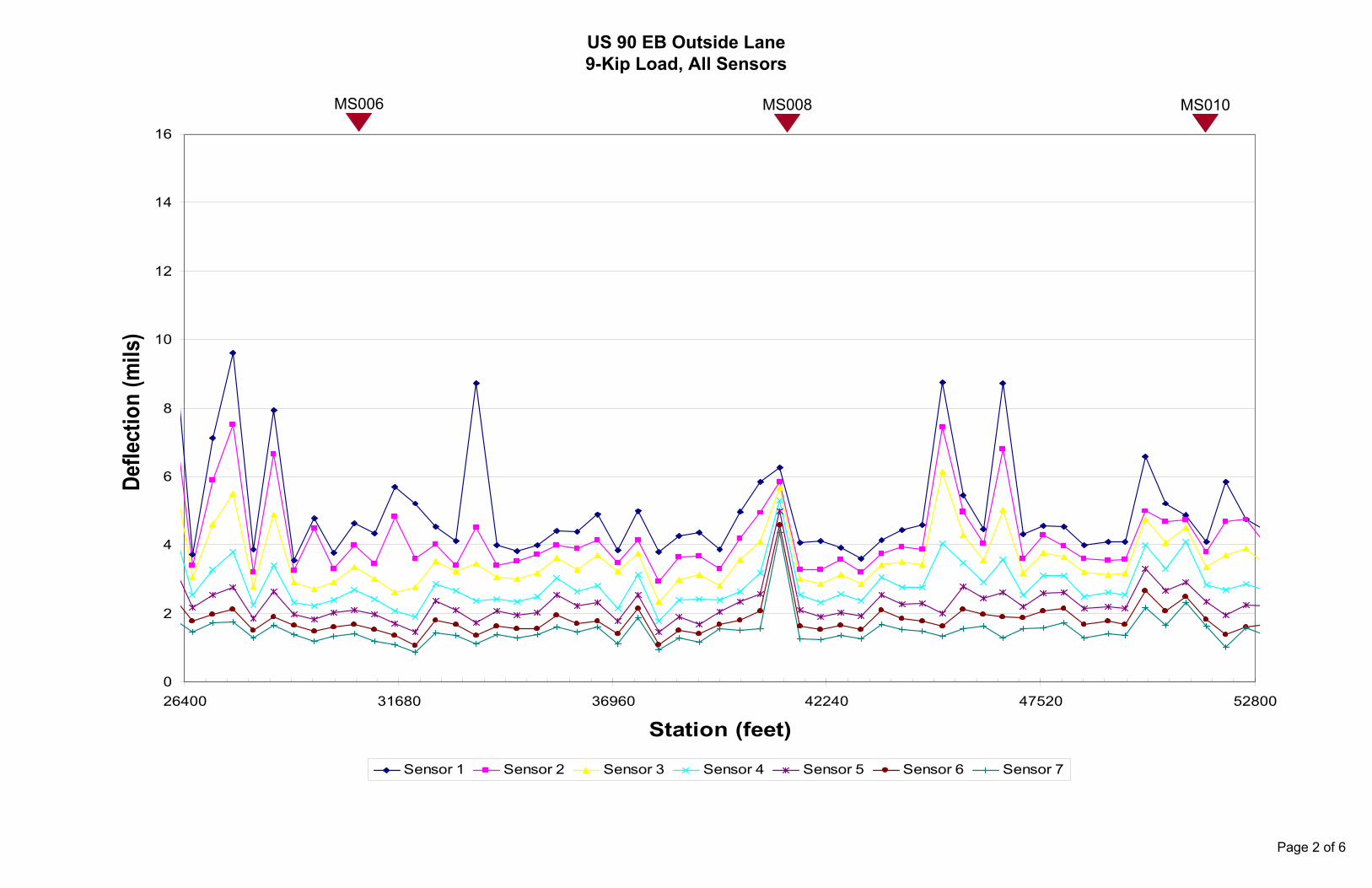
roadway was analyzed to identify those areas responding differently to loads. Deflection profile plots were produced for all sensors, as a quick preliminary analysis, to identify variability of the pavement and subgrade response. It should be noted that the Sensor No. 1 readings (the sensor directly under the load) are typically indicative of the overall strength of the pavement structure whereas the No. 7 readings (the sensor farthest away from the load) are more indicative of the subgrade characteristics. Tables 1-4 show the deflection statistics for each of the four passes. Data was subsectioned grouping consecutive FWD test locations with deflections of similar magnitude together. The deflection profile plots are included in Appendix A.


- 5 -

Table 1 – Deflection Statistics for Eastbound Inside Lane 9-kip Load

Direction Lane Stationing (ft) Statistic Sensor 1

(mils) Sensor 7

(mils) Average 5.36 1.47 Minimum 2.96 0.66 Maximum 11.52 3.33

3950 to 118700

Std. Dev. 1.43 0.37

Average 7.04 1.81 Minimum 4.70 1.13 Maximum 13.67 2.61

118700 to 130700

Std. Dev. 1.84 0.37


Eastbound Inside

130700 to 143700

Std. Dev. 1.05 0.33

Table 2 – Deflection Statistics for Eastbound Outside Lane

9-kip Load Direction Lane Stationing

(ft) Statistic Sensor 1 (mils)

Sensor 7 (mils)


4100 to 53850

Std. Dev. 1.78 0.50 Average 6.10 1.69 Minimum 3.72 0.97 Maximum 10.89 2.63

53850 to 83850


83850 to 105350


Eastbound Outside

105350 to 143600

Std. Dev. 2.28 0.49


- 6 -

Table 3 – Deflection Statistics for Westbound Inside Lane 9-kip Load

Direction Lane Stationing (ft) Statistic Sensor 1

(mils) Sensor 7

(mils) Average 6.50 1.71 Minimum 3.41 1.20 Maximum 10.61 2.70

3650 to 15900


15900 to 25900

Std. Dev. 1.23 0.27


25900 to 34900

Std. Dev. 4.01 0.47


34900 to 44900

Std. Dev. 1.05 0.24


44900 to 80400

Std. Dev. 2.89 0.56


80400 to 117900

Std. Dev. 1.89 0.50


117900 to 132400

Std. Dev. 2.28 0.52


Westbound Inside

132400 to 143150

Std. Dev. 1.32 0.37

Table 4 – Deflection Statistics for Westbound Outside Lane


- 7 -

9-kip Load Direction Lane Stationing

(ft) Statistic Sensor 1 (mils)

Sensor 7 (mils)


3800 to 26050

Std. Dev. 2.27 0.59


26050 to 53550

Std. Dev. 1.53 0.43


53550 to 82550

Std. Dev. 1.74 0.48


82550 to 111550

Std. Dev. 1.46 0.40


111550 to 130050

Std. Dev. 2.13 0.63


130050 to 138400

Std. Dev. 0.84 0.35


Westbound Outside

138400 to 143300

Std. Dev. 1.87 0.29

Backcalculation of the deflection data was performed to obtain layer moduli for each test

point. The pavement was analyzed to identify the load response at each test location using the non-destructive deflection testing data. Material properties and layer structure information was used to backcalculate layer moduli from the deflection data. The following two approaches outlined below were used in the analysis. Using both procedures enabled quality control


- 8 -

comparisons to be conducted to identify results that may warrant further evaluation or caution in use. Backcalculation of Subgrade Resilient Modulus (MR), Effective Pavement Modulus (Ep), Effective Structural Number (SNeff), and k-value from FWD Measurements, as Outlined in AASHTO 1993

The 1993 AASHTO Guide for Design of Pavement Structures outlines a method for calculating the subgrade resilient modulus and the effective modulus of all pavement layers above the subgrade using the measured deflection data.

The deflections measured at sufficiently large distances from the load (sensor 7) are

considered to be a reflection of the deformation of the subgrade layer only and hence can be used to compute the subgrade resilient modulus. Once the resilient modulus of the subgrade (MR) is estimated, the effective pavement modulus (Ep) can be calculated as a function of the deflection measured at the center of the FWD load plate (sensor 1), load plate pressure, radius of the load plate and thickness of the pavement layers above the subgrade (in concert with the MR). A temperature correction factor is incorporated in the relationship for the effective pavement modulus to account for the variations in the modulus of the asphalt concrete layer with temperature. A chart is used to determine the ratio Ep/MR. The effective pavement modulus (Ep) can then be calculated using the MR estimated in the first step of the procedure.

Our staff developed a tool to automatically perform these calculations when conducting a

network-level structural analysis for the Oklahoma DOT in 2005. The spreadsheet includes two methods for calculating Ep:

1. A graphical method, where the user estimates the Ep/MR ratio from a chart – following

exactly the method outlined in the 1993 AASHTO Guide. 2. A numerical method, which will provide the user directly with the Ep value. The numerical method was utilized due to the quantity of data being processed. Based

on the MR, Ep, and raw deflection data, we were also able to provide a structural number or k-value for each test point. Further details and specifics regarding the analysis and specific equations are included in Appendix B.

Tables 5-8 show the statistics of each of the structural parameters calculated for each of

the four passes. A discussion of the results shown on the tables is presented after Table 8. Table 5 – Structural Parameter Statistics for Eastbound Inside Lane


- 9 -

Direction Lane Stationing (ft) Statistic Ep

(psi) MR

(psi) SN k (pci)

kAREA (pci)

Average 1,302,272 25,890 4.70 334 326 Minimum 153,337 10,810 2.06 139 127 Maximum 9,281,755 54,328 7.67 700 656

3950 to 118700

Std. Dev. 924,326 6,383 0.96 83 82


118700 to 130750

Std. Dev. 634,330 4,652 0.85 60 67


Eastbound Inside

130700 to 143700

Std. Dev. 790,668 6,172 0.86 68 60

Table 6 – Structural Parameter Statistics for Eastbound Outside Lane


(psi) MR

(psi) SN k (pci)

kAREA (pci)


4100 to 53850

Std. Dev. 1,343,738 6,394 1.13 78 105 Average 1,525,729 22,161 4.88 285 305 Minimum 255,937 13,695 2.98 176 143 Maximum 6,073,810 36,945 7.19 476 521

53850 to 83850

Std. Dev. 985,720 4,498 1.01 58 86 Average 1,672,825 27,906 5.27 360 384 Minimum 161,775 9,319 2.52 120 9 Maximum 4,195,356 41,326 6.98 533 681

83850 to 105350

Std. Dev. 925,322 5,597 1.04 72 105 Average 1,411,452 23,385 4.95 303 292 Minimum 85,490 9,480 1.97 122 70 Maximum 5,257,880 46,786 7.03 603 574

Eastbound Outside

105350 to 143550

Std. Dev. 1,046,053 6,396 1.25 83 93

Table 7 – Structural Parameter Statistics for Westbound Inside Lane


- 10 -


(psi) MR

(psi) SN k (pci)

kAREA (pci)


36507 to 15900

Std. Dev. 1,118,701 4,593 1.22 60 88


15900 to 25900

Std. Dev. 732,656 6,814 0.90 88 91

Average 850,802 28,543 4.13 371 351 Minimum 63,487 13,913 1.88 179 215 Maximum 2,107,541 52,541 6.43 677 583

25900 to 34900

Std. Dev. 728,361 10,235 1.55 136 111


34900 to 44900

Std. Dev. 832,706 4,940 0.80 64 46


44887 to 80387

Std. Dev. 672,903 6,981 1.18 91 92


80400 to 117900

Std. Dev. 882,683 7,246 1.06 84 97


117900 to 132400

Std. Dev. 395,211 6,642 0.88 87 89


Westbound Inside

132400 to 143150

Std. Dev. 831,203 5,398 1.01 59 107

Table 8 – Structural Parameter Statistics for Westbound Outside Lane


- 11 -


(psi) MR

(psi) SN k (pci)

kAREA (pci)


3800 to 26050

Std. Dev. 851,000 6,453 1.28 83 97


26050 to 53550

Std. Dev. 806,086 6,577 1.04 85 81


53550 to 82550

Std. Dev. 739,495 4,866 1.04 63 86


82550 to 111550

Std. Dev. 901,334 6,722 1.10 87 129


111550 to 130050

Std. Dev. 640,309 6,934 1.08 92 100

Average 2,351,058 27,220 6.09 351 336 Minimum 1,174,511 17,138 4.70 221 151 Maximum 3,384,002 44,781 7.31 577 669

130050 to 138400

Std. Dev. 624,030 7,295 0.60 94 140


Westbound Outside

138400 to 143300

Std. Dev. 936,485 3,855 1.23 50 116

Average subgrade resilient modulus values backcalculated using the AASHTO method for

each section were consistent. The average over the entire roadway was about 25,000 psi, which is typical for a sand or stiff clay subgrade. The actual subgrade type was not specified in the core logs provided. The resilient modulus for the subgrade layer that is presented in Tables 5-8 is a backcalculated resilient modulus. The 1993 AASHTO Pavement Design Guide (Ref. 4)


- 12 -

recommends using a correction factor of 0.25 for backcalculated subgrade moduli for Portland cement concrete pavements. The backcalculated subgrade resilient modulus is 0.25 the design laboratory resilient modulus value. The structure for US 90 is a composite (AC/PCC) pavement.

The modulus of subgrade reaction (k-value) was computed using two procedures that are

both found in the 1993 AASHTO Guide. One was based on the subgrade resilient modulus and the other based on the AREA method (Appendix B goes into the details of each method). Values from the two methods are highly comparable. The minimum k-value for the eastbound direction is 268 and 259 pci, respectively for the two methods for the resilient modulus and AREA based k-values, and the maximum values are 360 and 384 pci, respectively. For the westbound direction values of 274 and 277 pci for the minimum k-value and 371 and 354 pci for the maximum k-value were obtained for the two methods, respectively. K-values between 200 and 300 pci are indicative of subgrades with high to very high levels of support. Table 9, from the Portland Cement Association, lists material types, typical level of support, and associated range of k-values for typical subgrade types (Ref. 5). While the calculated k-values for a specific material type may differ than the k-value range for a specific soil type as shown in Table 9, the table does present what level of support is expected for a given k-value.

Table 9 – Typical k-value Levels of Support

Type of Soil Level of Support k-value range

(pci)

Fine-grained soils in which silt and clay-size particles predominate

Low 75-120

Sands and sand-gravel mixtures with moderate amounts of silt and clay

Medium 130-170

Sands and sand-gravel mixtures relatively free of plastic fines

High 180-220

Cement-treated subbases Very High 250-400

The effective pavement modulus values calculated represent the overall modulus of all

layers above the subgrade layer. The expected effective pavement modulus for a composite pavement is between 1,000,000 and 3,000,000 psi. With the exception of four subsections in the westbound direction, all of the average effective pavement modulus values for each subsection were above 1 million psi. An area of particular concern is in the westbound inside lane for FWD test locations between 117,900 and 132,400 ft where the average value is 629,230 psi, which is over 200,000 psi less than the next lowest modulus value. This section also has the lowest


- 13 -

backcalculated moduli for the composite pavement structure as will be discussed in the next section.

Typically, structural numbers are only used to quantify the structure of flexible pavements.

As the structure of US 90 was a composite section with an AC surface, a structural number using deflection data was computed. Structural numbers ranged from between 4 and 6 over the entire length of roadway tested. There are localized areas of weakness with structural numbers as low as 1.7 and strong areas with structural numbers as high as 8.31. A review of the database provided will show the exact stations of localized areas of weakness and strength. The average structural number of the entire surveyed area is 4.93. The location of the lowest average structural number coincided with the lowest effective pavement modulus in the westbound inside lane between 117,900 and 132,400 ft, and on the eastbound inside lane between 118,700 and 130,750 ft, which also has the lowest effective pavement modulus and k-value for the eastbound direction. When the distributions of all effective pavement modulus values are examined, 36% of the test locations were less than 1,000,000 psi. For composite pavements, effective pavement modulus values of between 1- and 3,000,000 psi are expected. If traffic information were available, a structural number could be backcalculated to check the structural adequacy of each subsection in terms of allowable traffic over the pavement life.

Backcalculation Using Industry Standard Software

The FWD data was processed through industry standard backcalculation software developed in accordance with the ASTM standard D5858 (Standard Guide for Calculating In Situ Equivalent Elastic Moduli of Pavement Materials Using Layered Elastic Theory). Fugro used the MODCOMP (version 5) software developed at Cornell University for the backcalculation of layer moduli. This software was selected because it is well suited for processing large amounts of deflection data in numerous files using both a linear (Young’s Modulus) and non-linear (stress dependent elastic modulus) approach for materials characterization. Each data point was analyzed separately using its specific thickness to determine Young’s Modulus. Coring information and the GPR data for the layer structure and material property information were used for the backcalculation. Temperature correction was applied to the calculated HMAC surface modulus. An analysis using a non-linear approach may be conducted using the data collected. Table 10 provides the seed values used for the backcalculation. To facilitate the backcalculation process the AC and PCC layers were combined, using the seed values for PCC. The details for why this was done are included in Appendix B.


- 14 -

Table 10 – Backcalculation Seed Values

Layer Description Seed Modulus (psi) Poisson’s Ratio

Asphalt Concrete 650,000 0.35 Portland Cement Concrete 6,100,000 0.25

Subgrade 12,000 0.40

Fugro has developed an automated approach for summarizing this data. Our procedures

searched for outliers and those test points with unacceptable Percent Average Error per Sensor (PAES) for more detailed study and comparison. The modulus of subgrade reaction (k) for concrete pavements was also calculated, using the procedures outlined in the 1993 AASHTO Guide for Design of Pavement Structures (as part of our deliverables).

Quality control of the FWD analysis, as noted above, entails a detailed automated review

of the comparative results from the two procedures discussed above as well as the PAES noted from the backcalculation results. Points identified as outliers are reexamined to confirm the various inputs are valid (with obviously errant values edited) or suspect values revisited for possible clarification and explanation. Further details and specifics regarding the backcalculation analysis are included in Appendix B. Tables 11-14 provide the statistics of backcalculated moduli for the combined bound layers (AC and PCC) and the subgrade for each of the four passes including the subsections.


- 15 -

Table 11 – Backcalculated Moduli Statistics for Eastbound Inside Lane

Direction Lane Stationing (ft) Statistic

Backcalculated Composite Modulus

(psi)

Backcalculated Subgrade Modulus

(psi)

RMS Error (%)

Average 1,199,878 39,360 15.50 Minimum 152,000 8,560 4.04 Maximum 6,180,000 85,000 177.68

3950 to 118700

Std. Dev. 868,562 9,430 16.31


118700 to 130750

Std. Dev. 1,144,757 12,776 40.88


Eastbound Inside

130700 to 143700

Std. Dev. 561,469 7,979 3.46


- 16 -

Table 12 – Backcalculated Moduli Statistics for Eastbound Outside Lane



(psi)


(psi)

RMS Error (%)


4100 to 53850

Std. Dev. 1,072,952 11,603 6.61


53850 to 83850

Std. Dev. 761,068 9,447 6.34


83850 to 105350

Std. Dev. 1,202,592 12,108 16.48


Eastbound Outside

105350 to 143550

Std. Dev. 1,502,990 12,970 23.25


- 17 -

Table 13 – Backcalculated Moduli Statistics for Westbound Inside Lane



(psi)


(psi)

RMS Error (%)

Average 927,913 34,265 12.23 Minimum 152,000 18,900 8.59 Maximum 3,200,000 52,200 18.20

3650 to 15900

Std. Dev. 683,301 8,905 2.46


15900 to 25900

Std. Dev. 461,408 7,538 12.27


25900 to 34900

Std. Dev. 561,226 18,304 7.52


34900 to 44900

Std. Dev. 1,296,163 5,873 4.67


44900 to 80400

Std. Dev. 578,350 40,856 8.96


80400 to 117900

Std. Dev. 1,073,813 10,825 14.06


117900 to 132400

Std. Dev. 296,675 10,196 3.34


Westbound Inside

132400 to 143150

Std. Dev. 1,110,844 12,760 8.63


- 18 -

Table 14 – Backcalculated Moduli Statistics for Westbound Outside Lane



(psi)


(psi)

RMS Error (%)


3800 to 26050

Std. Dev. 1,107,662 11,034 13.78


26050 to 53550

Std. Dev. 729,182 8,407 12.75


53550 to 82550

Std. Dev. 551,514 8,960 2.97


82550 to 111550

Std. Dev. 1,210,131 13,193 7.25


111550 to 130050

Std. Dev. 437,231 12,933 14.21


130050 to 138400

Std. Dev. 765,134 18,923 4.06


Westbound Outside

138400 to 143300

Std. Dev. 896,056 12,044 7.89


- 19 -

The average backcalculated subgrade modulus values ranged from 30,000 to 50,000 psi. These values are on the high side of the range of expected values for a subgrade material, and represent a very good subgrade. Modulus values in this range are typical of a sandy subgrade or a very stiff clay subgrade. Subgrade type information was not included on the core logs.

The backcalculated composite modulus of the combined AC and PCC layers is essentially

an effective pavement modulus of all layers above the subgrade. This provides an overall stiffness of the pavement system as opposed to the individual pavement layers. (Appendix B includes an explanation of why a composite backcalculated modulus was reported.) As more variation was seen in the deflections of both lanes in the westbound direction than the eastbound direction, the backcalculated modulus results also reflect this variation.

Average backcalculated composite modulus values for the subsections identified ranged

from 1,200,000 to 1,700,000 psi in the eastbound direction and 500,000 to 1,800,000 psi in the westbound direction. Sections of roadway where the composite modulus values are less than 1 million psi were only in the westbound direction.

The westbound inside lane had four sections where the average modulus was less than

1,000,000 psi: 1) FWD test locations between 3,650 and 15,900 ft, 2) FWD test locations between 25,900 and 34,900 ft, 3) FWD test locations between 44,900 and 80,400 ft, and 4) FWD test locations between 117,900and 132,400 ft. The westbound outside lane had three sections where the modulus was less than 1,000,000 psi: 1) FWD test locations between 53,550 and 82,550 ft, 2) FWD test locations between 111,550 and 130,050 ft, and 3) FWD test locations between 138,400 and 143,300 ft. The areas of particular concern are in the westbound inside lane between 117,900 and 132,400 ft where the average modulus is 526,750 psi. For composite pavements an effective pavement modulus between 1,000,000 and 3,000,000 psi is expected. When looked at as a whole, 49% of all test points yielded a composite backcalculated modulus of less than 1,000,000 psi. A backcalculated composite modulus of 1,000,000 psi is at the lower end of the range of typical backcalculated moduli for composite pavements. This distribution was nearly the same for each of the individual passes. The subsections that have the lowest backcalculated composite modulus values correspond to the subsections with the lowest effective pavement modulus values. The values are based on separate types of data and processes, which reflect the differences in the moduli values; however, the trends in weakness and strength correlate very well.


- 20 -

GPR Data Processing and Reporting

Ground Penetrating Radar data was provided by EPIC, Inc. and for specifics of the GPR analysis and limitations of the GPR analysis, their report should be referred to. GPR data was provided for each lane. Thickness values were provided for the surface (AC) and subsurface (PCC) layers. Data was reported as average values over 25-ft intervals.

Upon receipt of the data, the Fugro office aligned the GPR data with the FWD data to allow for further analyses. The following steps were taken in this process of aligning the FWD and GPR data:

1) Global Positioning System (GPS) Coordinates were interpolated for any GPR data points

that did not have GPS coordinates from the GPR data points that did have GPS coordinates. This is valid for short straight distances between coordinates. As there were typically only one to two readings that required interpolation, distances were in the neighborhood of 50 to 75 ft between GPS readings, which is more than adequate to perform interpolation of GPS coordinates.

2) Based on the GPS coordinates at each FWD station thickness values were interpolated from the nearest two GPR data points. FWD points fell at or between each reported GPR thickness value at the 25 ft intervals.

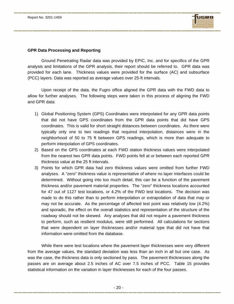
3) Points for which GPR data had zero thickness values were omitted from further FWD analyses. A “zero” thickness value is representative of where no layer interfaces could be determined. Without going into too much detail, this can be a function of the pavement thickness and/or pavement material properties. The “zero” thickness locations accounted for 47 out of 1127 test locations, or 4.2% of the FWD test locations. The decision was made to do this rather than to perform interpolation or extrapolation of data that may or may not be accurate. As the percentage of affected test point was relatively low (4.2%) and sporadic, the effect on the overall statistics and representation of the structure of the roadway should not be skewed. Any analyses that did not require a pavement thickness to perform, such as resilient modulus, were still performed. All calculations for sections that were dependent on layer thicknesses and/or material type that did not have that information were omitted from the database. While there were test locations where the pavement layer thicknesses were very different

from the average values, the standard deviation was less than an inch in all but one case. As was the case, the thickness data is only sectioned by pass. The pavement thicknesses along the passes are on average about 2.5 inches of AC over 7.5 inches of PCC. Table 15 provides statistical information on the variation in layer thicknesses for each of the four passes.


- 21 -

Table 15 – Thickness Statistics for Site

Direction Lane Statistic AC

Thickness (in.)

PCC Thickness

(in.)

Combined Thickness

(in.) Average 2.63 7.38 10.00 Minimum 1.15 3.97 7.38 Maximum 6.53 15.12 16.95

Inside

Std. Dev. 0.71 1.27 1.11 Average 2.69 7.37 10.06 Minimum 1.46 4.73 7.21 Maximum 6.51 9.92 12.32

Eastbound

Outside

Std. Dev. 0.84 0.93 0.97 Average 2.34 7.99 10.33

Minimum 1.62 5.64 8.07 Maximum 4.72 11.03 12.93

Inside

Std. Dev. 0.52 0.87 0.95 Average 2.63 7.86 10.49 Minimum 1.47 4.23 7.90 Maximum 6.35 11.87 13.77

Westbound

Outside

Std. Dev. 0.81 0.97 0.84

Analysis Database

A database that contains the raw deflection values and analysis results has been included. Table 16 shows the fields that are included in the database as well as the description of each field. This data description table is also included in the Access Database in the “Design View” of the table.

Table 16 – Data Descriptions Field Description

Sorter Used to Sort Data - Unique ID SectionID ID for FWD Pass

Direction Direction of FWD Pass

Lane Lane of FWD Pass

Fugro Field Sta. (ft) Fugro's Field DMI

MDOT Sta. (ft) Adjusted DMI to MDOT Stationing


- 22 -

Field Description

Surface Temp (F) Temperature of Pavement Surface

FWD Date Date of FWD Test

FWD Latitude Latitude at FWD Test

FWD Longitude Longitude of FWD Test

State Plane Northing State Plane Northing in Mississippi East Region

State Plane Easting State Plane Easting in Mississippi East Region

FWD Comment FWD Field Comment; Stations in this field match Fugro Field Sta.

Comment Description Description of Comment; Classifies Comments by Type

Stress (psi) Stress Load Plate on Ground During FWD Test

Force (lb) Load applied to pavement during FWD Test

D1 (mils) Deflection at sensor 1







AC Thickness (in.) Thickness of AC Layer

PCC Thickness (in.) Thickness of PCC Layer

MR (psi) Resilient Modulus Calculated Using AASHTO 1993

k = MR/19.4 (pci) k-value calculated using AASHTO 1993

keff static (pci) keff static (pci) - effective static k-value computed using AREA method from AASHTO 1993

Ep (psi) Effective Pavement Modulus Calculated Using AASHTO 1993

Ep/MR Ratio of Ep/MR

SN Structural Number Calculated Using AASHTO 1993

Backcalculated AC + PCC Modulus (psi) Composite Backcalculated Modulus of AC and PCC layer Combined

Backcalculated Subgrade Modulus (psi) Backcalculated Subgrade Modulus

RMS Error of Backcalculation RMS Error of Backcalculation

Combined AC + PCC Thickness (in.) Combined thickness of AC and PCC


- 23 -

CONCLUSION

When looking at the analysis results from the backcalculation analysis using Modcomp5 and the structural capacity analysis using procedures from the 1993 AASHTO Guide, between 36% and 49% of the pavement structure is performing weaker than what is expected for a composite pavement. Typically, composite pavements have a composite modulus of 1,000,000 to 3,000,000 psi. The 36% and 49% of the data points refer to the AASHTO analysis and the Modcomp5 backcalculation, respectively.

The other structural capacity parameters calculated are largely a function of the effective

pavement modulus and/or the backcalculated resilient modulus. The k-values, which were typically above 250 pci, are considered a good level of support. About half of the structural numbers calculated for the project were above a value of 5 and just above 75% were greater than 4. The structural number information can be more useful if traffic data is available. These uses include remaining life analysis and overlay thickness design.

From the analysis performed, the weaknesses that occur in the pavement structure

appear to be influenced more by the non-subgrade layers as opposed to the subgrade. Overall, subgrade resilient modulus and subgrade k-values were representative of moderately strong subgrades whereas weaknesses in the pavement were most evident in the effective pavement modulus and composite backcalculated modulus values, which take into account the contribution of the overlying layers in addition to the subgrade.

We appreciate the opportunity to assist with this pavement evaluation of structural

capacity. Our personnel are available if there are any questions. Electronic files of the data collected are provided with this report.

CONDITIONS

Since variation was found in the deflection readings, all parties involved should take notice that even more variation may be encountered between test locations. Statements in the report as to subsurface variation over given areas are intended only as estimations from the data obtained at test locations. The professional services that form the basis for this report have been performed using that degree of care and skill ordinarily exercised, under similar circumstances, by reputable pavement engineers practicing in the same locality. No other warranty, expressed or implied, is made as the professional advice set forth. Fugro's scope of work does not include the


- 24 -

investigation, detection, or design related to the presence of any biological pollutants. The term 'biological pollutants' includes, but is not limited to, mold, fungi, spores, bacteria, and viruses, and the byproducts of any such biological organisms. The results, conclusions, and recommendations contained in this report are directed at, and intended to be utilized within, the scope of work contained in the agreement executed by Fugro Consultants, Inc. and client. This report is not intended to be used for any other purposes. Fugro Consultants, Inc. makes no claim or representation concerning any activity or condition falling outside the specified purposes to which this report is directed, said purposes being specifically limited to the scope of work as defined in said agreement. Inquiries as to said scope of work or concerning any activity or condition not specifically contained therein should be directed to Fugro Consultants, Inc. for a determination and, if necessary, further investigation.


- 25 -

REFERENCES

1. Federal Highway Administration. 1992. Drainable Pavement Systems-Participant Notebook. (Demonstration Project 87). Publication No. FHWA-SA-92-008. Washington, DC: Federal Highway Administration.

2. Wyatt T., W. Barker, and J. Hall. 1998. Drainage Requirements in Pavements-Users

Manual. Publication No. FHWA-SA-96-070. Washington, DC: Federal Highway Administration.

3. Carpenter, S.H., M.I. Darter, B.J. Dempsey, and S. Herrin. 1981. A Pavement Moisture

Accelerated Distress (MAD) Identification System. Report FHWA/RD-81/079. Washington, DC: Federal Highway Administration.

4. “AASHTO Guide for Design of Pavement Structures 1993,” American Association of State

Highway and Transportation Officials, 1993, p. III-110. 5. Packard, Robert G., P.E., “Thickness Design for Concrete Highway and Street

Pavements,” Portland Cement Association, 1984, reprinted 1995, p. 24.


A P P E N D I X A

US 90 EB Inside Lane9-Kip Load, All Sensors

Page 1 of 6

MS001 MS003

0

2

4

6

8

10

12

14

16

0 5280 10560 15840 21120 26400

Station (feet)

Defle

ctio

n (m

ils)

Sensor 1 Sensor 2 Sensor 3 Sensor 4 Sensor 5 Sensor 6 Sensor 7

Page 2 of 6

MS005 MS009MS007

0

2

4

6

8

10

12

14

16

26400 31680 36960 42240 47520 52800

Station (feet)

Defle

ctio

n (m

ils)



Page 3 of 6

MS011 MS013

0

2

4

6

8

10

12

14

16

52800 58080 63360 68640 73920 79200

Station (feet)

Defle

ctio

n (m

ils)



Page 4 of 6

MS015 MS019MS017

0

2

4

6

8

10

12

14

16

79200 84480 89760 95040 100320 105600

Station (feet)

Defle

ctio

n (m

ils)



Page 5 of 6

MS021 MS023

0

2

4

6

8

10

12

14

16

105600 110880 116160 121440 126720 132000

Station (feet)

Defle

ctio

n (m

ils)



Page 6 of 6

MS027MS025

0

2

4

6

8

10

12

14

16

132000 137280 142560 147840 153120 158400

Station (feet)

Defle

ctio

n (m

ils)



US 90 EB Outside Lane9-Kip Load, All Sensors

Page 1 of 6

MS002 MS004

0

2

4

6

8

10

12

14

16

0 5280 10560 15840 21120 26400

Station (feet)

Defle

ctio

n (m

ils)


Page 2 of 6

MS006 MS010MS008

0

2

4

6

8

10

12

14

16

26400 31680 36960 42240 47520 52800

Station (feet)

Defle

ctio

n (m

ils)



Page 3 of 6

MS012 MS014

0

2

4

6

8

10

12

14

16

52800 58080 63360 68640 73920 79200

Station (feet)

Defle

ctio

n (m

ils)



Page 4 of 6

MS016 MS020MS018

0

2

4

6

8

10

12

14

16

79200 84480 89760 95040 100320 105600

Station (feet)

Defle

ctio

n (m

ils)



Page 5 of 6

MS022 MS024

0

2

4

6

8

10

12

14

16

105600 110880 116160 121440 126720 132000

Station (feet)

Defle

ctio

n (m

ils)



Page 6 of 6

MS028MS026

0

2

4

6

8

10

12

14

16

132000 137280 142560 147840 153120 158400

Station (feet)

Defle

ctio

n (m

ils)



US 90 WB Inside Lane9-Kip Load, All Sensors

Page 1 of 6

MS055 MS053

0

2

4

6

8

10

12

14

16

0 5280 10560 15840 21120 26400

Station (feet)

Defle

ctio

n (m

ils)


Page 2 of 6

MS051 MS047MS049

0

2

4

6

8

10

12

14

16

26400 31680 36960 42240 47520 52800

Station (feet)

Defle

ctio

n (m

ils)



Page 3 of 6

MS045 MS043

0

2

4

6

8

10

12

14

16

52800 58080 63360 68640 73920 79200

Station (feet)

Defle

ctio

n (m

ils)



Page 4 of 6

MS041 MS037MS039

0

2

4

6

8

10

12

14

16

79200 84480 89760 95040 100320 105600

Station (feet)

Defle

ctio

n (m

ils)



Page 5 of 6

MS035 MS033

0

2

4

6

8

10

12

14

16

105600 110880 116160 121440 126720 132000

Station (feet)

Defle

ctio

n (m

ils)



Page 6 of 6

MS029MS031

0

2

4

6

8

10

12

14

16

132000 137280 142560 147840 153120 158400

Station (feet)

Defle

ctio

n (m

ils)



US 90 WB Outside Lane9-Kip Load, All Sensors

Page 1 of 6

MS056 MS054

0

2

4

6

8

10

12

14

16

0 5280 10560 15840 21120 26400

Station (feet)

Defle

ctio

n (m

ils)


Page 2 of 6

MS052 MS048MS050

0

2

4

6

8

10

12

14

16

26400 31680 36960 42240 47520 52800

Station (feet)

Defle

ctio

n (m

ils)



Page 3 of 6

MS046 MS044

0

2

4

6

8

10

12

14

16

52800 58080 63360 68640 73920 79200

Station (feet)

Defle

ctio

n (m

ils)



Page 4 of 6

MS042 MS038MS040

0

2

4

6

8

10

12

14

16

79200 84480 89760 95040 100320 105600

Station (feet)

Defle

ctio

n (m

ils)



Page 5 of 6

MS036 MS034

0

2

4

6

8

10

12

14

16

105600 110880 116160 121440 126720 132000

Station (feet)

Defle

ctio

n (m

ils)



Page 6 of 6

MS030MS032

0

2

4

6

8

10

12

14

16

132000 137280 142560 147840 153120 158400

Station (feet)

Defle

ctio

n (m

ils)




A P P E N D I X B

In addition to the backcalculation of moduli using Modcomp5, the following additional parameters were provided to MDOT.

1) The calculation of the subgrade resilient modulus (MR) and effective pavement modulus (Ep) as outlined in the AASHTO 1993 Guide for Design of Pavement Structures. The MR and Ep calculated were based on the deflections at Sensors 1 (0 in. from load plate) and 7 (60 in. from load plate).

a. A temperature correction factor was incorporated when computing the Effective Pavement Modulus to account for variations in the asphalt modulus due to temperature. (There is both a graphical and a numeric method for calculating Ep. For processing the data, the numeric method will be reported. But the tools for using both methods can be provided to MDOT.)

2) Modulus of subgrade reaction, k-value, for concrete pavements. 3) Effective Structural Number (SNeff) based on deflections for flexible pavements.

General Comments Regarding the Layer Backcalculation Analysis Layer moduli values were backcalculated using Modcomp5. The pavement structure for the entire project was a composite pavement with an AC layer overlying a PCC layer. No base layer was considered for the backcalculation. This resulted in a three-layer system for analysis: AC over PCC over subgrade. After running an initial analysis, it was evident that the AC layer above the PCC layer was not producing reasonable moduli values. This is not uncommon for composite pavements where an AC layer overlays a PCC layer. The AC modulus values were unrealistically high. This resulted in a different approach being taken in the backcalculation analysis. Instead of backcalculating the individual moduli values of each of the bound (AC and PCC) layers, the bound layer thicknesses were combined and then the backcalculation analysis was repeated. As the PCC layer was the dominant layer in the deflections, the send modulus and Poisson’s ratio for PCC were used to represent the combined bound layer material properties. Backcalculated moduli values were much more reasonable for a composite pavement. The modulus represented when combining of layers during backcalculation is essentially an effective pavement modulus of the bound layers above the subgrade. General Comments Regarding the Structural Capacity Parameter Analysis One of the primary issues encountered in applying the AASHTO guide to compute the above values is how to analyze pavements with AC over PCC. Three typical types of pavement structures may be encountered:

1) AC pavements over a non-PCC layer

2) PCC pavements over any layer type 3) Composite Pavements (AC overlays over a PCC pavement)

For computation purposes regarding the SN and k-value, these cases are handled as such (refer to case definitions above):

1) Only an SN calculated 2) Only a SN and k-value calculated 3) Only a SN and k-value calculated

All pavements will have the MR and Ep calculated. The MR and Ep are calculated based on the deflections at Sensor 1 (0 in. from load plate) and Sensor 7 (72 in. from load plate). The only pavement type that was tested on US90 for MDOT was a composite pavement. Case 3 from above was applied when analyzing the data. Computation of MR and Ep - Limitations The MR of subgrade and the Ep that are computed based on deflection from the 1993 AASHTO Design Guide page III-97.

P = load dr = deflection at radius r r = radius

There are reduction factors to the Backcalculated MR values to convert them to laboratory MR values used in the 1993 AASHTO Pavement Design Guide. (For AC, a factor of 0.33 is used to obtain the design (laboratory) resilient modulus and for PCC this factor is 0.25). The analysis that we are performing to calculate Ep uses the unaltered MR value. These factors are found in the sections where the deflection methods for determining a subgrade resilient modulus are discussed (AASHTO Design Guide pg. III-101 and III-111). The k-value computation for rigid pavements will incorporate the 0.25 reduction factor for the MR for PCC pavements. For the computation of Ep, the deflection at d0 is used and requires a temperature correction to adjust the deflection. The deflections are adjusted to 68° F. Two classes of systems are considered in the AASHTO Design Guide for Flexible Pavements (AASHTO III-97 for flexible and III-109 for rigid).

1) AC over Granular or Asphalt Treated Base 2) AC over Cement- or Pozzolanic-Treated Base

The computation of Ep for Rigid pavements does not require a temperature correction.

rdPM

rR

24.0=

AC over PCC is not mentioned in the AASHTO Guide. To account for sections where AC over PCC is present, the PCC can be considered a Cement Treated base when calculating the temperature correction factor. Iterating the Ep value until the calculated deflection matches the corrected field deflection will find a solution for Ep. This can be done easily in Microsoft Excel using the Solver function. The equation used is in the AASHTO Design Guide on page III-97 (III-109 for rigid).

d0 = deflection at center of load at 680 F in inches (calculated deflection) p = NDT plate pressure in psi a = NDT plate radius in inches (5.91 in.) D = total thickness of pavement layers above subgrade in inches MR = subgrade resilient modulus in psi Ep = effective pavement modulus of all layers above subgrade in psi

The field deflection at d=0 will be corrected to 68° F using Figures 5.6 or 5.7 from the AASHTO Design Guide pages III-99 and III-100. Equations are derived from these two graphs so that the conversion factors could be programmed. [Note: The equations are fitted to the curves to perform the double interpolation in order to obtain the temperature correction factor for the deflection at Sensor 1. This double interpolation requires a thickness and a temperature, which is part of the field data.] The curves used to generate equations for the computation of the temperature correction factor are valid for certain temperature and asphalt thickness ranges. It is expected the limits of asphalt thickness and temperature may be exceeded at times (although less frequently than the thickness). For values of either temperature or thickness that exceed the maximum limit used to generate the equations, the maximum limit will be used instead. Using values beyond the limit often result in corrected deflections that are either negative or unrealistically small. This is a mathematical issue inherent due to the curve fitting process. The models will be tested through comparison to the graphs they were generated from to verify they are within the temperature and thickness limits of the graphs. To ensure that temperature correction factors will be within a reasonable range, for temperatures above 120° F, 120° F is used, and for AC thicknesses greater than 12 in., 12 in. is

+

−

+

+

=p

R

pR

EaD

ME

aDM

pad

2

2

3

0

1

11

1

15.1

used. Based on prior experience, when AC pavements above 12 in. thick only need to be corrected for temperature in the top 12 in. of the layer. Computation of SNeff from Deflection Testing Two procedures exist for determining the SNeff for flexible pavements. SNeff from deflections (Ep, MR) The effective structural number can be calculated using the computed effective pavement modulus. The equation is as follows. The Ep in this equation is from the Ep calculated from the deflections (see above). This equation is found in the AASHTO Guide on page III-102. An alternative to the equation is Figure 5.8 on page III-103. The guide describes both the equation and Figure 5.8 to be used for AC pavements.

30045.0 peff EDSN =

[Note: The procedure for the Ep and MR are the same for flexible and rigid pavements. The only difference is this last step, the SN calculation, which is not specified for PCC pavements. This equation can be applied to rigid pavements, but must be used with caution as the equation was developed for flexible pavements. Computation of k-value The procedure used to compute a k-value was based on the AASHTO Design Guide Section 3.2.1 pg. II-37-44. As the [PCC] slab is directly on the subgrade, the following equation was used. This obtained a composite k-value.

4.19RMk =

The k-value was also computed using the AREA method. This method for backcalculating a dynamic effective k-value from NDT that can be converted to a static effective k-value (keffstatic) is a

variation of the procedure 3 above from the 1993 AASHTO Guide, III-117 and III-131. It can be used for PCC, and AC over PCC pavements. This adapted procedure is found on page L-13 to L-21.

- The deflection bowl AREA is computed for either PCC or AC/PCC pavements. A

correction will be need to be applied to the AC/PCC modulus to the deflection at 0 in. if necessary. These correction equations are straightforward and are found on page L-19. One is for unbonded and the other for bonded interfaces between the AC and PCC.

- Next, the dense liquid radius of relative stiffness, lk, is calculated as an intermediate step in obtaining the dynamic effective k-value. The lk is a function of the AREA.

- From the lk, load, d0, Euler’s constant, and plate radius, the dynamic effective k-value can be calculated. This equation is on page L-14.

- To obtain the static effective k-value the dynamic effective k-value is divided by two. - To apply this method, a bonded AC/PCC interface was assumed and a AC modulus of

500,000 psi.

Documents

REPORT FOR PAVEMENT TESTING AND ANALYSIS OF …mdot.ms.gov/documents/research/Reports/Interim and Final Reports... · Mississippi Department of Transportation ... Summary Report for