Embed Size (px)
Citation preview

i
MDOT PAVEMENT MANAGEMENT SYSTEM
PREDICTION MODELS AND FEEDBACK SYSTEM
FINAL REPORT
by
K.P. George
Conducted by the
DEPARTMENT OF CIVIL ENGINEERINGTHE UNIVERSITY OF MISSISSIPPI
in corporation with the
MISSISSIPPI DEPARTMENT OF TRANSPORTATION
and the
U. S. DEPARTMENT OF TRANSPORTATIONFEDERAL HIGHWAY ADMINISTRATION
The University of MississippiUniversity, Mississippi
October 2000

Technical Report Documentation Page1.Report No.
FHWA/MS-DOT-RD-00-119
2. Government Accession No.
3. Recipient’s Catalog No.
5. Report Date
October 20004. Title and Subtitle
MDOT Pavement Management System: Prediction Models andFeedback System 6. Performing Organization Code
7. Author(s)
K. P. George8. Performing Organization Report No.
MS-DOT-RD-00-11910. Work Unit No. (TRAIS)
9. Performing Organization Name and Address
University of MississippiDepartment of Civil EngineeringUniversity, MS 38677 11. Contract or Grant No.
State Study 11913. Type Report and Period Covered
Final – August 1995 to October 2000
12. Sponsoring Agency Name and Address
Mississippi Department of TransportationResearch DivisionPO Box 1850Jackson, MS 39215-1850
14. Sponsoring Agency Code
15. Supplementary Notes
16. AbstractAs a primary component of a Pavement Management System (PMS), prediction models are crucial for one or more of the following analyses:maintenance planning, budgeting, life-cycle analysis, multi-year optimization of maintenance works program, and authentication of designalternatives. The main focus of the study is to develop pavement deterioration models. Four cycles of pavement condition data and the requiredinventory data are compiled from the Mississippi Department of Transportation (MDOT) PMS database. Though regression is the primary tool fordeveloping models, Bayesian regression is also employed whenever feasible. Expert opinion regarding the major distresses in pavements arecompiled, augmenting the field data. The study begins with a review of relevant literature with the aim of identifying the commonly employedexplanatory variables and various model forms.
Five pavement families are identified for the model development: original flexible, overlaid flexible, composite, jointed concrete, and continuouslyreinforced concrete pavements. Models for each family are developed for predicting distresses, roughness, and a composite condition index(Pavement Condition Rating). The database employed is divided into ‘in-sample’ data constituting a major portion (70 percent) with ‘out-of-sample’data comprising the remaining. Totally 26 models are developed, with the in-sample data: six each for original flexible, overlaid flexible, andcomposite, and four each for jointed concrete and continuously reinforced concrete pavements. The models are subsequently verified with the ‘out-of-sample’ data.
Among the scores of model forms attempted, power form or some variation of it fits all of the models while satisfying crucial boundary conditions.The out-of-sample data provides an independent database to verify the validity of the models. A sensitivity analysis of the model equation ispresented in each case, substantiating the predictive capability of the model. In seven cases, incorporating expert opinion in the field data, employingBayesian regression, resulted in better prediction models. While these equations form a nucleus for condition prediction of MDOT pavementnetwork, for project level analyses, a shift adjustment of the prediction should be made to match the current observation.
The feedback program developed in this study computes load index of original pavements of all types and overlaid flexible pavements. Load indexis the ratio of the actual ESAL sustained by the pavement and the design ESAL. Also included is a routine to verify/substantiate the predictionmodels by comparing the actual to the predicted distresses.17. Key Words
Prediction Model, Performance Model, DistressModel, Pavement Management, Condition Data,Feedback System.
18. Distribution Statement
19. Security Classif. (of this report)
Unclassified20. Security Classif. (of this page)
Unclassified21. No. of Pages 22. Price
Form DOT F 1700.7 (8-72)
Reproduction of completed page authorized

ii
ACKNOWLEDGMENTS
This report includes the results of a study titled, “MDOT Pavement Management
System: Prediction Models and Feedback System”, conducted by the Department of Civil
Engineering, The University of Mississippi, in cooperation with the Mississippi
Department of Transportation (MDOT) and the U.S. Department of Transportation, Federal
Highway Administration.
The author wishes to thank Joy Portera of the MDOT Research Division for their
excellent cooperation and technical input in the project study. James Watkins, also of the
MDOT Research Division, had assisted the researcher in compiling condition data in a
form that can be directly used for model building. The condition data collected by
PaveTech© and Pathway Services, Inc. was ably supervised by MDOT Research Division
Staff. Thanks are due to engineers from MDOT Headquarters and the Districts who
volunteered their time to compile the expert opinion matrix.
A. Rajashekaran and Ashraf El-Rahim were the key personnel developing models
and in the report writing phase as well. Jianrong Yu assisted in developing regression
models. Sherra Jones ably typed the final report.
DISCLAIMER
The opinions, findings and conclusions expressed in this report are those of the
author and not necessarily those of the Mississippi Department of Transportation or the
Federal Highway Administration. This does not constitute a standard, specification or
regulation.

iii
ABSTRACT
As a primary component of a Pavement Management System (PMS), prediction
models are crucial for one or more of the following analyses: maintenance planning,
budgeting, life-cycle analysis, multi-year optimization of maintenance works program, and
authentication of design alternatives. The main focus of the study is to develop pavement
deterioration models. Four cycles of pavement condition data and the required inventory
data are compiled from the Mississippi Department of Transportation (MDOT) PMS
database. Though regression is the primary tool for developing models, Bayesian
regression is also employed whenever feasible. Expert opinions regarding the major
distresses in pavements were compiled, augmenting the field data. The study begins with a
review of relevant literature with the aim of identifying the commonly employed
explanatory variables and various model forms.
Five pavement families are identified for the model development: original
flexible, overlaid flexible, composite, jointed concrete, and continuously reinforced
concrete pavements. Models for each family are developed for predicting distresses,
roughness, and a composite condition index (Pavement Condition Rating). The database
employed is divided into ‘in-sample’ data constituting a major portion (70 percent) with
‘out-of-sample’ data comprising the remaining. Totally 26 models are developed, with the
in-sample data: six for original flexible, six for overlaid flexible, six for composite, and
four each for jointed concrete and continuously reinforced concrete pavements. The
models are subsequently verified with the ‘out-of-sample’ data.
Among the scores of model forms attempted, power form or some variation of it
fits all of the models while satisfying crucial boundary conditions. The out-of-sample data

iv
provides an independent database to verify the validity of the models. A sensitivity
analysis of the model equation is presented in each case, substantiating the predictive
capability of the model. In seven cases, incorporating expert opinion in the field data,
employing Bayesian regression resulted in better prediction models. While these equations
form a nucleus for condition prediction of MDOT pavement network, for project level
analyses, a shift adjustment of the prediction should be made to match the current
observation.
The feedback program developed in this study computes load index of original
pavements of all types and overlaid flexible pavements. Load index is the ratio of the
actual ESAL sustained by the pavement and the design ESAL. Also included is a routine to
verify/substantiate the prediction models by comparing the actual to the predicted
distresses.

v
METRIC CONVERSION CHART
To convert U.S. units to metric units, the following conversion factors should be used:
Multiply U.S. Units By To Obtain Metric Units
mils 0.0254 millimeters (mm)
inches (in) 2.5400 centimeters (cm)
feet (ft) 0.3048 meters
yards (yd) 0.9144 meters (m)
square inches (in2) 6.4516 square centimeters (cm2)
square feet (ft2) 0.0929 square meters (m2)
square yards (yd2) 0.8361 square meters (m2)
cubic inches (in3) 16.3872 cubic centimeters (cm3)
cubic feet (ft3) 0.0283 cubic meters (m3)
cubic feet (ft3) 28.3162 liters (1)
cubic yards (yd3) 0.7646 cubic meters (m3)
gallons (gal) 3.7854 liters (1)
pounds (lbs) 0.4536 kilograms (kgs)
pounds (lbs) 453.592 grams (g)
ounces (oz) 28.3495 grams (g)
pounds per kilograms persquare inch (psi) 0.0703 cubic meter (kgs/cm2)
pounds per kilograms percubic foot (lbs/ft3) 16.091 cubic meter (kgs/m3)
miles per hour (mph) 1.609 kilometers per hour (km/hr)
degrees Fahrenheit (ºF) degrees Celsius (ºC)minus 32º 5/9 ºC = 5/9 (ºF-32º)
British thermal units (BTU) 252.0 calories (cal)TABLE OF CONTENTS

vi
1. INTRODUCTION . . . . . . . . . . . . . . . . . . . . . . . . . . . . . . . . . . . . . . . . . . . . . . . . 11.1 General . . . . . . . . . . . . . . . . . . . . . . . . . . . . . . . . . . . . . . . . . . . . . . . . . . . . . . . 1
1.2 Pavement Management System . . . . . . . . . . . . . . . . . . . . . . . . . . . . . . . . . . . . 11.3 Prediction Models . . . . . . . . . . . . . . . . . . . . . . . . . . . . . . . . . . . . . . . . . . . . . . 41.4 Manifestation of Pavement Distresses. . . . . . . . . . . . . . . . . . . . . . . . . . . . . . . .6
1.4.1 Asphalt Concrete Pavement Distresses . . . . . . . . . . . . . . . . . . . . . .61.4.2 Jointed Concrete Pavement Distresses . . . . . . . . . . . . . . . . . . . . . . 71.4.3 Continuously Reinforced Concrete Pavement Distresses . . . . . . . 8
1.5 Feedback System. . . . . . . . . . . . . . . . . . . . . . . . . . . . . . . . . . . . . . . . . . . . . . . 91.6 Objectives of the Study. . . . . . . . . . . . . . . . . . . . . . . . . . . . . . . . . . . . . . . . . . 111.7 Scope of the Study. . . . . . . . . . . . . . . . . . . . . . . . . . . . . . . . . . . . . . . . . . . . . .11
2. REVIEW OF THE LITERATURE . . . . . . . . . . . . . . . . . . . . . . . . . . . . . . . . .142.1 Introduction . . . . . . . . . . . . . . . . . . . . . . . . . . . . . . . . . . . . . . . . . . . . . . . . . . .142.2 Regression Models . . . . . . . . . . . . . . . . . . . . . . . . . . . . . . . . . . . . . . . . . . . . . 14
2.2.1 Requirements for a Reliable Regression. . . . . . . . . . . . . . . . . . . . 162.2.2 Review of Prediction Models. . . . . . . . . . . . . . . . . . . . . . . . . . . . .18
2.2.2.1 Asphalt Surfaced Pavement Deterioration Models. . . . . . 192.2.2.1.1 Models for Prediction of Cracks. . . . . . . . . . . 192.2.2.1.2 Models for Prediction of Rutting. . . . . . . . . . .232.2.2.1.3 Models for Prediction of Roughness. . . . . . . . 25
2.2.2.2 Rigid Pavement Deterioration Models. . . . . . . . . . . . . . . 272.2.2.3 Models for Prediction of Composite Condition Index. . . 302.2.2.4 Other Model Types. . . . . . . . . . . . . . . . . . . . . . . . . . . . . .37
2.2.3 Bayesian Regression. . . . . . . . . . . . . . . . . . . . . . . . . . . . . . . . . . . 39
3. PMS DATABASE AND DATA FOR MODELING. . . . . . . . . . . . . . . . . . . . 403.1 Introduction. . . . . . . . . . . . . . . . . . . . . . . . . . . . . . . . . . . . . . . . . . . . . . . . . . . 403.2 Description of Database. . . . . . . . . . . . . . . . . . . . . . . . . . . . . . . . . . . . . . . . . 413.3 Pavement Family Approach. . . . . . . . . . . . . . . . . . . . . . . . . . . . . . . . . . . . . . 463.4 Response Variables. . . . . . . . . . . . . . . . . . . . . . . . . . . . . . . . . . . . . . . . . . . . 48
3.4.1 Response Variables in Asphalt Surfaced Pavements. . . . . . . . . . .483.4.2 Response Variables in Jointed Concrete Pavements. . . . . . . . . . 49
3.4.3 Response Variables in Continuously Reinforced ConcretePavements . . . . . . . . . . . . . . . . . . . . . . . . . . . . . . . . . . . . . . . . . . 49
3.5 Identification of Explanatory Variables. . . . . . . . . . . . . . . . . . . . . . . . . . . . . 51
4. MODELING METHOLOGY . . . . . . . . . . . . . . . . . . . . . . . . . . . . . . . . . . . . . 594.1 Introduction . . . . . . . . . . . . . . . . . . . . . . . . . . . . . . . . . . . . . . . . . . . . . . . . . . 594.2 Regression Modeling Techniques . . . . . . . . . . . . . . . . . . . . . . . . . . . . . . . . . 60
4.2.1 Multiple Linear Forms. . . . . . . . . . . . . . . . . . . . . . . . . . . . . . . . . 604.2.2 Nonlinear Regression. . . . . . . . . . . . . . . . . . . . . . . . . . . . . . . . . . .61
4.2.2.1 Power Form. . . . . . . . . . . . . . . . . . . . . . . . . . . . . . . . . . . . 624.3 Modeling by Bayesian Regression. . . . . . . . . . . . . . . . . . . . . . . . . . . . . . . . . .62
5. MODELS, RESULTS, AND DISCUSSIONS. . . . . . . . . . . . . . . . . . . . . . . . . . 67

vii
5.1 General . . . . . . . . . . . . . . . . . . . . . . . . . . . . . . . . . . . . . . . . . . . . . . . . . . . . . . 675.2 Original Flexible Pavement Models . . . . . . . . . . . . . . . . . . . . . . . . . . . . . . . 68
5.2.1 Medium and High Severity Alligator Cracking Model(WCAMH) . . . . . . . . . . . . . . . . . . . . . . . . . . . . . . . . . . . . . . . . . .69
5.2.2 Model for ‘Other Cracks’ (OC). . . . . . . . . . . . . . . . . . . . . . . . . . .765.2.3 Model for ‘Other Cracks’ of Medium and High Severity’
(OCMH). . . . . . . . . . . . . . . . . . . . . . . . . . . . . . . . . . . . . . . . . . . . .785.2.4 Rutting Model. . . . . . . . . . . . . . . . . . . . . . . . . . . . . . . . . . . . . . . . 785.2.5 Roughness Model. . . . . . . . . . . . . . . . . . . . . . . . . . . . . . . . . . . . . .825.2.6 PCR Model . . . . . . . . . . . . . . . . . . . . . . . . . . . . . . . . . . . . . . . . . 83
5.3 Overlaid Flexible Pavement Models. . . . . . . . . . . . . . . . . . . . . . . . . . . . . . . . 865.3.1 Medium and High Severity Alligator Cracking Model. . . . . . . . .86
5.3.2 Model for Other Cracks. . . . . . . . . . . . . . . . . . . . . . . . . . . . . . . . .905.3.3 Model for Other Cracks of Medium and High Severity. . . . . . . . 90
5.3.4 Rutting Model. . . . . . . . . . . . . . . . . . . . . . . . . . . . . . . . . . . . . . . . 925.3.5 Roughness Model. . . . . . . . . . . . . . . . . . . . . . . . . . . . . . . . . . . . . .945.3.6 PCR Model. . . . . . . . . . . . . . . . . . . . . . . . . . . . . . . . . . . . . . . . . . 96
5.4 Composite Pavement Models. . . . . . . . . . . . . . . . . . . . . . . . . . . . . . . . . . . . . 995.4.1 Medium and High Severity Alligator Cracking Model. . . . . . . .100
5.4.2 Other Cracks Model. . . . . . . . . . . . . . . . . . . . . . . . . . . . . . . . . . 1025.4.3 Model for Other Cracks of Medium and High Severity. . . . . . . 102
5.4.4 Rutting Model. . . . . . . . . . . . . . . . . . . . . . . . . . . . . . . . . . . . . . . 1045.4.5 Roughness Model. . . . . . . . . . . . . . . . . . . . . . . . . . . . . . . . . . . . .1065.4.6 PCR Model . . . . . . . . . . . . . . . . . . . . . . . . . . . . . . . . . . . . . . . . 106
5.5 Models for Jointed Concrete Pavements . . . . . . . . . . . . . . . . . . . . . . . . . . . 1095.5.1 Model for Cracking . . . . . . . . . . . . . . . . . . . . . . . . . . . . . . . . . . 1115.5.2 Spalling Model . . . . . . . . . . . . . . . . . . . . . . . . . . . . . . . . . . . . . . 1115.5.3 Roughness Model . . . . . . . . . . . . . . . . . . . . . . . . . . . . . . . . . . . 1135.5.4 PCR Model . . . . . . . . . . . . . . . . . . . . . . . . . . . . . . . . . . . . . . . . 115
5.6 Continuously Reinforced Concrete Pavement Models. . . . . . . . . . . . . . . . . 1175.6.1 Model for Cracks. . . . . . . . . . . . . . . . . . . . . . . . . . . . . . . . . . . . .1195.6.2 Punchout Model . . . . . . . . . . . . . . . . . . . . . . . . . . . . . . . . . . . . . 1195.6.3 Roughness Model.. . . . . . . . . . . . . . . . . . . . . . . . . . . . . . . . . . . .1225.6.4 PCR Model . . . . . . . . . . . . . . . . . . . . . . . . . . . . . . . . . . . . . . . . 122
5.7 Project Level Distress/Performance Prediction …. . . . . . . . . . . . . . . . . . . . . 1245.8 Engineering Feedback System . . . . . . . . . . . . . . . . . . . . . . . . . . . . . . . . . . . .1265.9 Summary . . . . . . . . . . . . . . . . . . . . . . . . . . . . . . . . . . . . . . . . . . . . . . . . . . . .128
5.9.1 Summary of Significant Variables for each Pavement Family . .130
6. SUMMARY AND CONCLUSIONS . . . . . . . . . . . . . . . . . . . . . . . . . . . . . . 1316.1 Summary. . . . . . . . . . . . . . . . . . . . . . . . . . . . . . . . . . . . . . . . . . . . . . . . . . . .131
6.1.1 Regression Models. . . . . . . . . . . . . . . . . . . . . . . . . . . . . . . . . . . .1316.2 Conclusions. . . . . . . . . . . . . . . . . . . . . . . . . . . . . . . . . . . . . . . . . . . . . . . . . . 1336.3 Implementation. . . . . . . . . . . . . . . . . . . . . . . . . . . . . . . . . . . . . . . . . . . . . . . 1346.4 Benefits. . . . . . . . . . . . . . . . . . . . . . . . . . . . . . . . . . . . . . . . . . . . . . . . . . . . . 135

viii
REFERENCES. . . . . . . . . . . . . . . . . . . . . . . . . . . . . . . . . . . . . . . . . . . . . . . . . . . . . . . .136
APPENDIXPavement Rehabilitation Strategy Selection Decision Trees. . . . . . . . . . . . . . . .143

ix
LIST OF TABLES
3.1 Distresses in different types of pavements (Adapted fromSHRP LTPP 10). . . . . . . . . . . . . . . . . . . . . . . . . . . . . . . . . . . . . . . . . . . . . . . . . . .44
3.2 Significant data elements in the SHRP National Information ManagementSystem for pavements with asphalt concrete surfaces (42) . . . . . . . . . . . . . . . . ..52
3.3 Significant data elements in the SHRP National Information ManagementSystem for pavements with Portland cement concrete surfaces (42) . . . . . . . . . 53
3.4 Factors affecting pavement condition. . . . . . . . . . . . . . . . . . . . . . . . . . . . . . . . . . 53
5.1 Range of response variables used in the development of models,Original flexible pavements. . . . . . . . . . . . . . . . . . . . . . . . . . . . . . . . . . . . . . . . . .69
5.2 Range of explanatory variables used in the development of models,Original flexible pavements. . . . . . . . . . . . . . . . . . . . . . . . . . . . . . . . . . . . . . . . . .69
5.3 Field data for medium and high severity alligator cracks (WCAMH)in three families of pavements. . . . . . . . . . . . . . . . . . . . . . . . . . . . . . . . . . . . . . . .72
5.4 Field data for Other Cracks (OC) and medium and high severity Other Cracks(OCMH) in three families of pavement. . . . . . . . . . . . . . . . . . . . . . . . . . . . . . . . .72
5.5 Range of response variables employed in the development of models,Overlaid flexible pavements . . . . . . . . . . . . . . . . . . . . . . . . . . . . . . . . . . . . . . . . .86
5.6 Range of explanatory variables used in the development of models,Overlaid flexible pavements . . . . . . . . . . . . . . . . . . . . . . . . . . . . . . . . . . . . . . . . 88
5.7 Range of response variables employed in the development of models,Composite pavements . . . . . . . . . . . . . . . . . . . . . . . . . . . . . . . . . . . . . . . . . . . . . .99
5.8 Range of explanatory variables used in the development of models,Composite pavements. . . . . . . . . . . . . . . . . . . . . . . . . . . . . . . . . . . . . . . . . . . . . 100
5.9 Range of response variables used in the development of models,Jointed concrete pavements . . . . . . . . . . . . . . . . . . . . . . . . . . . . . . . . . . . . . . . . 109
5.10 Range of explanatory variables used in the development of models,Jointed concrete pavements . . . . . . . . . . . . . . . . . . . . . . . . . . . . . . . . . . . . . . . . 111
5.11 Range of response variables used in the development of models,Continuously reinforced concrete pavements . . . . . . . . . . . . . . . . . . . . . . . . . . .117

x
5.12 Range of explanatory variables used in the development of models,Continuously reinforced concrete pavements. . . . . . . . . . . . . . . . . . . . . . . . . . . 117
6.1 Models for original flexible pavements. . . . . . . . . . . . . . . . . . . . . . . . . . . . . . . .132
6.2 Models for overlaid flexible pavements . . . . . . . . . . . . . . . . . . . . . . . . . . . . . . 132
6.3 Models for composite pavements. . . . . . . . . . . . . . . . . . . . . . . . . . . . . . . . . . . . 133
6.4 Models for jointed concrete pavements . . . . . . . . . . . . . . . . . . . . . . . . . . . . . . . 133
6.5 Models for continuously reinforced concrete pavements. . . . . . . . . . . . . . . . . . 133

xi
LIST OF FIGURES
1.1 Illustration of MDOT-PMS development and implementationprogram. . . . . . . . . . . . . . . . . . . . . . . . . . . . . . . . . . . . . . . . . . . . . . . . . . . . . . . . . . 3
3.1 Determination of 85th percentile rutting. . . . . . . . . . . . . . . . . . . . . . . . . . . . . . . . .50
4.1 Typical power form curves. . . . . . . . . . . . . . . . . . . . . . . . . . . . . . . . . . . . . . . . . . 63
4.2 Encoding matrix for Pavement Condition Rating (PCR).Original flexible pavement. . . . . . . . . . . . . . . . . . . . . . . . . . . . . . . . . . . . . . . . . . 66
5.1 Comparison of medium and high severity alligator cracks(WCAMH) predicted by data-model, expert model andposterior model in flexible original pavement. . . . . . . . . . . . . . . . . . . . . . . . . . . .73
5.2 Comparison of the normal probability plots of log(CESAL). Flexible original pavement. . . . . . . . . . . . . . . . . . . . . . . . . . . . . . . . . 75
5.3 Variation of medium and high severity alligator cracks(WCAMH) with age for a range of traffic levels. Flexibleoriginal pavement, (MSN=5) . . . . . . . . . . . . . . . . . . . . . . . . . . . . . . . . . . . . . . . . 77
5.4 Variation of other cracks (OC) with age for a range oftraffic levels. Flexible original pavement, (MSN=5). . . . . . . . . . . . . . . . . . . . . .79
5.5 Variation of medium and high severity other cracks (OCMH)with age for a range of traffic levels. Flexible originalpavement. . . . . . . . . . . . . . . . . . . . . . . . . . . . . . . . . . . . . . . . . . . . . . . . . . . . . . . . 79
5.6 Comparison of rutting prediction using data- expert- and posteriormodels. Flexible original pavement with yearly ESAL=200,000 . . . . . . . . . . . . .81
5.7 Variation of International Roughness Index (IRI) with age fora range of traffic levels. Flexible original pavement, MSN=5). . . . . . . . . . . . . . 81
5.8 Comparison of measured and predicted Pavement ConditionRating using original flexible pavement out-of-sample data. . . . . . . . . . . . . . . . 84
5.9 Comparison of Pavement Condition Rating (PCR) estimated byexperts and predicted by data-models. Yearly ESAL=200,000. . . . . . . . . . . . . .85
5.10 Comparison of measured and predicted medium and high severityAlligator cracks (WCAMH) using out-of-sample data.Overlaid flexible pavement. . . . . . . . . . . . . . . . . . . . . . . . . . . . . . . . . . . . . . . . . . 87

xii
5.11 Variation of medium and high severity alligator cracks (WCAMH)with age for a range of traffic levels using data-model. Overlaid
flexible pavement, (MSN=4, RES=10). . . . . . . . . . . . . . . . . . . . . . . . . . . . . . . . 89
5.12 Variation of medium and high severity alligator cracks (WCAMH)with age for a range of traffic levels using posterior model.Overlaid flexible pavement, (MSN=4). . . . . . . . . . . . . . . . . . . . . . . . . . . . . . . . . 89
5.13 Comparison of measured and predicted other cracks (OC) usingout-of-sample data. Overlaid flexible pavement. . . . . . . . . . . . . . . . . . . . . . . . .91
5.14 Variation of other cracks (OC) with age for a range of trafficlevels using data-model. Overlaid flexible pavement,(TOPTHK=50.8mm, RES=10). . . . . . . . . . . . . . . . . . . . . . . . . . . . . . . . . . . . . . . 91
5.15 Comparison of measured and predicted medium and high othercracks (OCMH) using out-of-sample data. Overlaid flexiblepavement. . . . . . . . . . . . . . . . . . . . . . . . . . . . . . . . . . . . . . . . . . . . . . . . . . . . . . . . 93
5.16 Variation of medium and high other cracks (OCMH) with age for arange of traffic levels using data-model. Overlaid flexible
pavement, (TOPTHK=50.8mm, RES=10). . . . . . . . . . . . . . . . . . . . . . . . . . . . . . 93
5.17 Variation of 85th percentile rutting (RT85) with age for a rangeof traffic levels using Bayesian model. Overlaid flexiblepavement. . . . . . . . . . . . . . . . . . . . . . . . . . . . . . . . . . . . . . . . . . . . . . . . . . . . . . . 95
5.18 Comparison of measured and predicted International RoughnessIndex (IRI) using out-of-sample data. Overlaid flexiblepavement. . . . . . . . . . . . . . . . . . . . . . . . . . . . . . . . . . . . . . . . . . . . . . . . . . . . . . . .97
5.19 Variation of International Roughness Index (IRI) with age for arange of traffic levels using data-model. Overlaid flexiblepavement, (MSN=4, TOPTHK=50.8mm, RES=10). . . . . . . . . . . . . . . . . . . . . . . 97
5.20 Comparison of measured and predicted Pavement ConditionRating (PCR) using out-of-sample data. Overlaid flexiblepavement. . . . . . . . . . . . . . . . . . . . . . . . . . . . . . . . . . . . . . . . . . . . . . . . . . . . . . . . 98
5.21 Variation of Pavement Condition Rating (PCR) with age for a rangeof traffic levels using data-model. Overlaid flexible pavement,(MSN=4, TOPTHK=50.8mm, RES=10) . . . . . . . . . . . . . . . . . . . . . . . . . . . . . . .98
5.22 Variation of medium and high severity alligator cracks (WCAMH)with age for a range of traffic levels using data-modelComposite pavement, (TOPTHK=50.8) . . . . . . . . . . . . . . . . . . . . . . . . . . . . . . .101

xiii
5.23 Variation of medium and high severity alligator cracks (WCAMH)with age for a range of traffic levels using Bayesian model.Composite pavement, (TOPTHK=50.8). . . . . . . . . . . . . . . . . . . . . . . . . . . . . . . 101
5.24 Comparison of measured and predicted other cracks (OC) usingout-of-sample data. Composite pavement . . . . . . . . . . . . . . . . . . . . . . . . . . . . . 103
5.25 Variation of other cracks (OC) with age for a range of trafficlevels using data model. Composite pavement, (TOPTHK=50.8mm) . . . . . . . 103
5.26 Comparison of measured and predicted medium and high othercracks (OCMH) using out-of-sample data. Composite pavement. . . . . . . . . . . 105
5.27 Variation of medium and high other cracks (OCMH) with age for arange of traffic levels using data-model. Composite pavement,(TOPTHK=50.8mm). . . . . . . . . . . . . . . . . . . . . . . . . . . . . . . . . . . . . . . . . . . . . . 105
5.28 Variation of 85th percentile rutting (RT85) with age for a range oftraffic levels using Bayesian model. Composite pavement,(TOPTHK=50.8mm). . . . . . . . . . . . . . . . . . . . . . . . . . . . . . . . . . . . . . . . . . . . . . 107
5.29 Comparison of measured and predicted roughness, IRI, usingout-of-sample data. Composite pavement. . . . . . . . . . . . . . . . . . . . . . . . . . . . . .108
5.30 Variation of roughness, IRI, with age for a range of traffic levelsusing data-model. Composite pavement, (TOPTHK=50.8mm). . . . . . . . . . . . .108
5.31 Comparison of measured and predicted Pavement Condition Rating(PCR) using out-of-sample data. Composite pavement. . . . . . . . . . . . . . . . . . . 110
5.32 Variation of Pavement Condition Rating (PCR) with age for arange of traffic levels using data-model. Composite pavement,(TOPTHK=50.8mm). . . . . . . . . . . . . . . . . . . . . . . . . . . . . . . . . . . . . . . . . . . . . . 110
5.33 Comparison of measured and predicted all cracks (AC) using out-of-sampledata. Jointed concrete pavement. . . . . . . . . . . . . . . . . . . . . . . . . . . . . . . . . . . . .112
5.34 Variation of all cracks (AC) with age for a range of traffic levelsusing data-model. Jointed concrete pavement, (SLABTHK=254mm). . . . . . . .112
5.35 Comparison of measured and predicted spalling (SP) using out-of-sample data. Jointed concrete pavement . . . . . . . . . . . . . . . . . . . . . . . . . . . . . . 114
5.36 Variation of spalling (SP) with age for a range of traffic levels usingdata-model. Jointed concrete pavement. . . . . . . . . . . . . . . . . . . . . . . . . . . . . . . 114

xiv
5.37 Comparison of measured and predicted International RoughnessIndex (IRI) using out-of-sample data. Jointed ConcretePavement. . . . . . . . . . . . . . . . . . . . . . . . . . . . . . . . . . . . . . . . . . . . . . . . . . . . . . .116
5.38 Variation of International Roughness Index (IRI) with age for arange of traffic levels using data-model. Jointed concrete
pavement, (SLABTHK=254mm). . . . . . . . . . . . . . . . . . . . . . . . . . . . . . . . . . . . 116
5.39 Variation of Pavement Condition Rating (PCR) with age for arange of traffic levels, using Bayesian model. Jointed concretepavement. . . . . . . . . . . . . . . . . . . . . . . . . . . . . . . . . . . . . . . . . . . . . . . . . . . . . . . 118
5.40 Variation of all cracks (AC) with age for a range of traffic levelsusing Bayesian model. Continuously reinforced concretepavement . . . . . . . . . . . . . . . . . . . . . . . . . . . . . . . . . . . . . . . . . . . . . . . . . . . . . . .120
5.41 Variation of punchouts (PO) with age for a range of traffic levelsusing Bayesian model. Continuously reinforced concretepavement . . . . . . . . . . . . . . . . . . . . . . . . . . . . . . . . . . . . . . . . . . . . . . . . . . . . . . .120
5.42 Comparison of measured and predicted International RoughnessIndex (IRI) using out-of-sample data. Continuously reinforcedconcrete pavement . . . . . . . . . . . . . . . . . . . . . . . . . . . . . . . . . . . . . . . . . . . . . . . 123
5.43 Variation of International Roughness Index (IRI) with age for arange of traffic levels using data-model. Continuouslyreinforced concrete pavement. . . . . . . . . . . . . . . . . . . . . . . . . . . . . . . . . . . . . . . 123
5.44 Variation of Pavement Condition Rating (PCR) with age for arange of traffic levels using Bayesian model. Continuouslyreinforced concrete pavement . . . . . . . . . . . . . . . . . . . . . . . . . . . . . . . . . . . . . . .125
5.45 The horizontal-shift model adjustment . . . . . . . . . . . . . . . . . . . . . . . . . . . . . . . .127
5.46 The vertical-shift model adjustment . . . . . . . . . . . . . . . . . . . . . . . . . . . . . . . . . .127
A.1 Rehabilitation Strategy Selection Tree for Flexible and CompositePavements . . . . . . . . . . . . . . . . . . . . . . . . . . . . . . . . . . . . . . . . . . . . . . . . . . . . . 145
A.2 Schematic Diagram Showing the Dominant Strategy Selection . . . . . . . . . . . . .147
A.3 Rehabilitation Strategy Selection Decision Tree for Jointed (plainand reinforced) Concrete Pavements. . . . . . . . . . . . . . . . . . . . . . . . . . . . . . . . . .148
A.4 Rehabilitation strategy selection decision tree for continuously

xv
reinforced concrete pavements. . . . . . . . . . . . . . . . . . . . . . . . . . . . . . . . . . . . . . 149

1
CHAPTER 1
INTRODUCTION
1.1 GENERAL
With a large network of highways in place, the need for preservation and efficient
maintenance of existing highways is growing. To find cost-effective strategies for
providing, evaluating, and maintaining pavements in a serviceable condition, highway
agencies are resorting to Pavement Management Systems (PMSs). However, with
pavements deteriorating continually, preserving and managing pavements has become a
complex task. The problem is further compounded by the fact that the funds available for
maintenance and rehabilitation are dwindling. Maintenance at a given time necessitates the
evaluation of pavement condition. The present condition of a network can be evaluated by
condition surveys. For efficient and economical maintenance of pavements, not only the
present condition but also the future condition of pavements should be considered.
Prediction of future pavement condition, therefore, is a key component of a Pavement
Management System.
1.2 PAVEMENT MANAGEMENT SYSTEM
A Pavement Management System helps in making informed decisions enabling the
maintenance of the network in a serviceable and safe condition at a minimum cost to both
the agency and the road users. To adequately meet this requirement, well-documented
information is essential to make defensible decisions on the basis of sound principles of
engineering and management. The objective of establishing a PMS is to improve the
efficiency of this decision making, expand its scope, provide feedback about the
consequences of decisions, and ensure consistency of decisions made at different levels

2
within an organization. The elements and products of a Pavement Management System
include:
• an inventory of pavements in the network,
• a database of information pertinent to past and current pavement condition,
• an analysis program which, among other things, makes use of prediction models for
forecasting pavement condition in the future or in the design horizon
• long range budgeting provisions
• prioritizing the annual work program,
• a basis for communication of the agency’s plans,
• a feedback system.
The modules of the PMS (2) adopted by the Mississippi Department of Transportation
(MDOT), with the logical structure, are shown in Figure 1. The basic modules include:
• A database that contains inventory, condition, traffic, and historical data
• A Pavement Analysis Program (PAP), which determines the condition of a pavement
and selects a maintenance action based on its condition and other criteria. Also, it
establishes an annual work program and estimates the budget required. A number of
reports are generated from the analysis.
Many other modules are established which supply the necessary inputs for the PMS
analysis. Deterioration models, maintenance and rehabilitation policies, their unit costs,
and vehicle operating costs are such inputs. Deterioration models, which form an
important element of PMS analysis, comprise this study.
Thus, a Pavement Management System can be applied in the areas of planning,

3

4
budgeting, scheduling, performance evaluation, and research. It can be used for
prioritization, funding, setting strategies, selecting alternatives, identifying problem areas,
simplifying communications with the legislature, and providing general and specific
information which is useful to decision makers and management. All these activities of a
PMS use deterioration models.
1.3 PREDICTION MODELS
A pavement deterioration model or prediction model is a “mathematical
description of the expected values that a pavement attribute will take during a specified
analysis period” (3). An attribute is a property of a pavement section or class of
pavements that provides a significant measure of the behavior, performance, adequacy,
cost, or value of the pavement (3). In other words, it is a mathematical description that can
be used to predict future pavement deterioration based on the present pavement condition,
deterioration factors, and the effect of maintenance (4).
The importance of accurate prediction of future pavement condition cannot be over-
emphasized as it affects many other components of a Pavement Management System.
Prediction models are indispensable for many processes of decision-making as they are
useful in establishing answers to the questions of what, where, and when, with respect to
maintenance actions. Simply put, the prediction models enable us to determine the type of
maintenance treatment to be adopted, the portions of the network requiring treatment, and
the timing of the maintenance actions. Life-cycle analysis and evaluation of rehabilitation
alternatives can be performed using the prediction models. Used at network level,
pavement deterioration models are helpful in planning, programming, and budgeting.
Budget analyses include the following:

5
• Estimating the funds required to bring the total network from its current condition
level to a desired condition level
• Estimating the budget required to maintain the network at specific levels of
performance over multiple years
• Prioritizing projects when the available funding is less than that required to meet
specific performance objectives.
Also, the ability to predict future pavement conditions can lead to the development
of multi-year, network-level optimal maintenance actions. Prediction models permit
increased understanding of pavement behavior so that steps can be taken to reduce the
development of distress or to extend the service life of pavements. This includes an
evaluation of cost-effectiveness of pavement maintenance treatments. Evaluation and
refinement of design procedures are possible utilizing prediction models.
Other uses of prediction models at the network level include studies on pavement
costs for different legal vehicle weights, sizes, tire pressures, and suspension systems,
determination of equitable permit fees for overweight vehicles, etc. Since these network
level usage predictions affect the level of taxation and fees, they form a rational basis for
all public investments in highway transportation.
At the project level, prediction models are used to design pavements, to perform
life-cycle cost analyses, to select optimal designs with least total costs, and in trade-off
analyses in which the annualized costs of new construction, maintenance, rehabilitation,
and user costs are considered for a specific pavement design. Simply put, prediction
models affect a wide spectrum of services within a Pavement Management System. Better

6
prediction models make a better Pavement Management System, which leads to
considerable cost savings (5-9).
1.4 MANIFESTATION OF PAVEMENT DISTRESSES
Typically, the deterioration of a pavement is represented by the development of
distresses leading to a reduction in serviceability and/or structural breakdown of the
pavement. Distress itself is a physical manifestation of damage caused to a pavement by
loadings, environmental factors, etc. There are different kinds of distresses identified for
various types of pavements. The Strategic Highway Research Program (SHRP)(10) lists
15 distress types for asphalt concrete surfaced pavements, sixteen for jointed concrete
surfaced pavements, and fifteen for continuously reinforced concrete surfaced pavements.
Relying on this, MDOT has adopted a short list of distresses, which are tabulated in
reference (11). Besides being useful for condition evaluation, they play a vital role in
rehabilitation selection. The decision trees for maintenance selection, developed for the
MDOT, can be seen in the Appendix. Selected distresses/distress groups for each
pavement type are entered in the decision tree to arrive at the appropriate rehabilitation
action.
The listed distresses in the decision tree for each pavement type are briefly
described:
1.4.1 Asphalt Concrete Surfaced Pavement Distresses
The asphalt concrete (ASP) surfaced pavement types include:
• original flexible pavements; i.e., asphalt pavements in their first performance
period
• overlaid flexible pavements

7
• composite pavements; i.e., asphalt concrete overlays over Portland cement
concrete pavements
For ASP pavements, cracking and rutting are the primary distresses that detract from
serviceability.
Alligator Cracking. Alligator, fatigue, or map cracking is a series of
interconnecting cracks caused by fatigue of asphalt concrete surface under repeated traffic
loadings. Cracking begins at the bottom of the asphaltic layer where tensile stress/strain is
highest under a wheel load. The cracks propagate to the surface initially as a series of
parallel longitudinal cracks. Under repeated traffic they develop into many-sided, sharp-
angled pieces into a pattern resembling chicken wire or the skin of an alligator. It is
measured in square feet of surface area.
Other Cracks: These cracks include low severity alligator cracking, block
cracking, edge cracking, longitudinal cracking, and transverse cracking (10), measured in
square feet of surface area.
Rutting: A rut is a longitudinal surface depression in the wheel paths. Rutting
arises from permanent deformation in any of the pavement layers or subgrade, usually
caused by consolidation or lateral movement of the materials due to traffic load. Thus,
densification (decrease in volume and, hence, increase in density), and shear deformation
lead to rutting. It is usually measured by average depth in inches or millimeters.
1.4.2 Jointed Concrete Pavement Distresses
The distresses considered in jointed concrete pavements (JCP) are cracking and
spalling.
Cracking: Cracks in jointed concrete pavements include durability or “D” cracking,
longitudinal cracking, and transverse cracking. These cracks are caused by many factors,

8
such as loading, temperature, other environmental actions, and poor workmanship/quality
of materials. The length of the cracks on a pavement are measured and recorded. The
cracks are assumed to have influence on a pavement width of one foot. Accordingly, the
area of pavement affected by cracks is obtained by multiplying length of cracks by one.
Spalling: Spalling is cracking, breaking, chipping, or fraying of slab edges or
cracked edges. A spall usually angles downward to intersect a joint or a crack, and is
caused by excessive loading caused by traffic or by infiltration of incompressible
materials. It is usually measured in length and converted into the area affected.
1.4.3 Continuously Reinforced Concrete Pavement Distresses
Punchouts and cracks are the major distresses considered in the decision trees for
Continuously Reinforced Concrete (CRC) pavements.
Punchout: A punchout is an area enclosed by two closely spaced transverse cracks,
a short longitudinal crack, and the edge of the pavement or a longitudinal joint. It also
includes “Y” cracks that exhibit spalling, breaking, and faulting. This distress is caused by
heavy repeated loads, inadequate slab thickness, loss of foundation support, and/or a
localized concrete construction deficiency. It is recorded as number of punchouts per
kilometer.
Cracks: The cracks in CRC pavements include durability, longitudinal, and
transverse cracks. These are caused by loading, shrinkage, temperature effects, and other
environmental factors. These cracks are measured as the area of the pavement affected.
In addition to the above-mentioned distresses, two other attributes of pavement
deterioration requiring prediction models for all the three types of pavements include
roughness, expressed in International Roughness Index (IRI), and a condition index,
expressed in terms of Pavement Condition Rating (PCR).
9
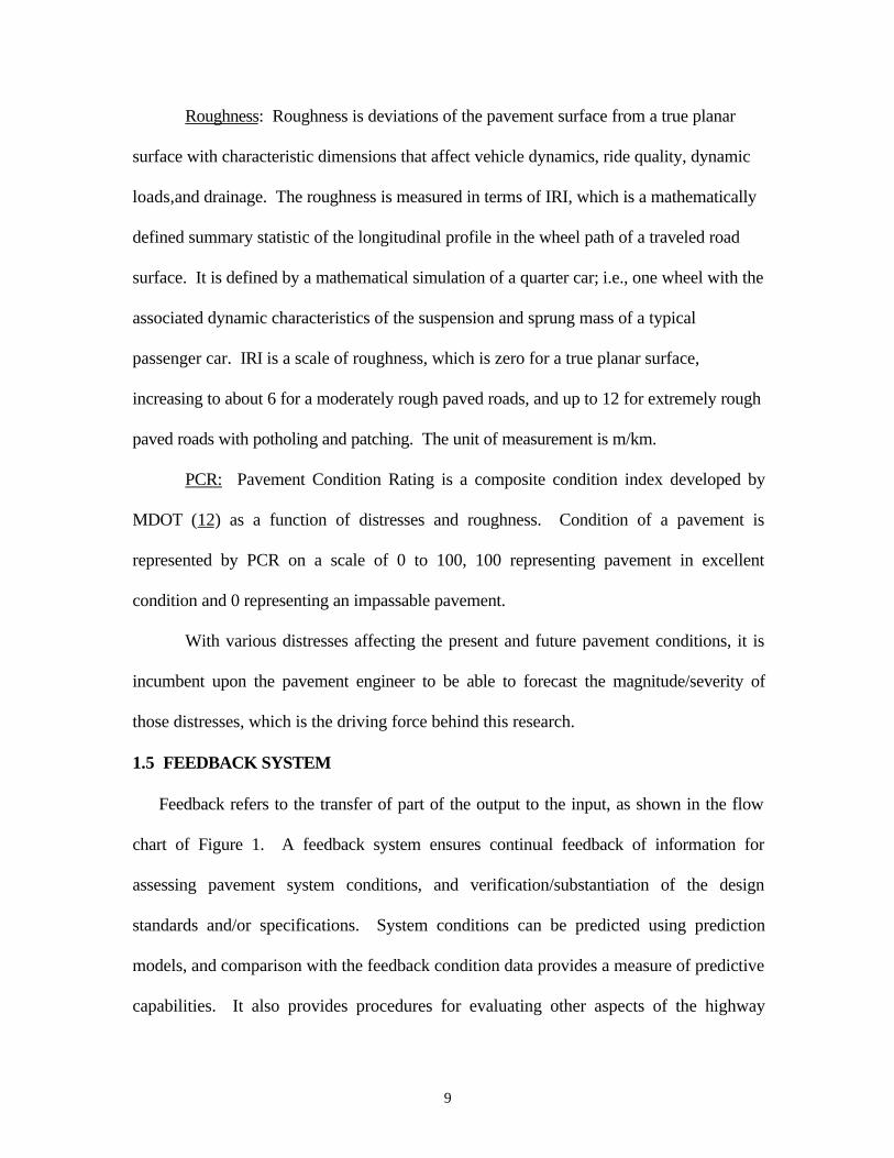
Roughness: Roughness is deviations of the pavement surface from a true planar
surface with characteristic dimensions that affect vehicle dynamics, ride quality, dynamic
loads,and drainage. The roughness is measured in terms of IRI, which is a mathematically
defined summary statistic of the longitudinal profile in the wheel path of a traveled road
surface. It is defined by a mathematical simulation of a quarter car; i.e., one wheel with the
associated dynamic characteristics of the suspension and sprung mass of a typical
passenger car. IRI is a scale of roughness, which is zero for a true planar surface,
increasing to about 6 for a moderately rough paved roads, and up to 12 for extremely rough
paved roads with potholing and patching. The unit of measurement is m/km.
PCR: Pavement Condition Rating is a composite condition index developed by
MDOT (12) as a function of distresses and roughness. Condition of a pavement is
represented by PCR on a scale of 0 to 100, 100 representing pavement in excellent
condition and 0 representing an impassable pavement.
With various distresses affecting the present and future pavement conditions, it is
incumbent upon the pavement engineer to be able to forecast the magnitude/severity of
those distresses, which is the driving force behind this research.
1.5 FEEDBACK SYSTEM
Feedback refers to the transfer of part of the output to the input, as shown in the flow
chart of Figure 1. A feedback system ensures continual feedback of information for
assessing pavement system conditions, and verification/substantiation of the design
standards and/or specifications. System conditions can be predicted using prediction
models, and comparison with the feedback condition data provides a measure of predictive
capabilities. It also provides procedures for evaluating other aspects of the highway

10
network, including observed life cycle costs and performance of rehabilitation treatments
and of different pavement types. Identification of deleterious aggregates/materials is
another area where feedback analysis can be extremely useful. In summary, a feedback
system provides for measurement and evaluation of performance of the system in service.
In the context of a PMS, the on-going monitoring information is brought to bear on
the initial input, making such comparisons as follows (11).
• Comparisons of actual costs of maintenance, rehabilitation, and reconstruction
(available through contract bids and agency records) with those used in the PMS
analysis.
• Evaluations of field observations of pavement conditions with those predicted by
PMS models.
• Contrasts between actual performance standards achieved and those specified in
the PMS analysis.
This report covers the development of prediction models and compilation of a
feedback system. Heavy reliance is placed on historical data for developing both of these
modules. That is, the main input for both subsystems is the historical database, such as
condition history, pavement structure history, and deflection history, if available.
1.6 OBJECTIVES OF THE STUDY
The primary objective of this study is to develop models that predict pavement
performance. Two categories of models will be developed. The first category includes
distress prediction models for five families of pavement: original flexible, flexible with

11
overlay, composite, jointed concrete, and continuously reinforced concrete. Performance
such as PCR prediction models for both asphalt surfaced and concrete pavements comprise
the second category. Whenever feasible, regression models are augmented with expert
opinion employing Bayesian regression. A second objective is to design/develop a stand-
alone feedback module to be used in the MDOT pavement management system. Three sub-
modules comprising the main module, are the following:
• Load index ratio of flexible, jointed concrete and CRC pavements
• Load index ratio of overlaid flexible pavements
• Verification of distresses by comparing the actual to the predicted
1.7 SCOPE OF THE STUDY
The MDOT-PMS has adopted a decision tree approach, based on
distresses/distress groups, for the selection of maintenance actions. Models are sought for
these distresses/distress groups and for MDOT’s performance index (PCR) for both
asphalt surfaced and concrete pavements. Three categories of asphalt-surfaced pavements
are recognized for this purpose:
• original flexible pavements, i.e., pavements in their initial performance cycle,
• overlaid flexible pavements
• composite pavements.
Concrete pavements are classified into two groups:
• jointed concrete
• continuously reinforced concrete pavements.
As dictated by the rehabilitation selection decision trees, for each category of
asphalt-surfaced pavement, six models are sought:

12
1. Area of alligator cracks of medium and high severity, percent
2. Area of ‘other cracks’ (combination of low severity alligator, block, edge,
longitudinal, transverse, and reflection cracks), percent
3. Percent of medium and high severity ‘other cracks’ expressed as a
percentage of total (low, medium, and high severity)
4. Eighty-fifth percentile rutting, mm
5. Roughness, IRI, m/km.
6. Pavement condition rating, on a scale of 0 to 100
For jointed concrete pavements, four distress models are to be developed:
1. Area of cracks (corner, D, longitudinal, and transverse cracks), percent
2. Area of spalling (longitudinal and transverse), percent
3. Roughness, IRI, m/km.
4. Pavement condition rating, on a scale of 0 to 100
The models required for continuously reinforced concrete pavements include:
1. Area of cracks (longitudinal and transverse), percent
2. Punchouts, #/km
3. Roughness, IRI, m/km.
4. Pavement condition rating, on a scale of 0 to 100
These models would become an integral part of the pavement management systems.
Current as well as future rehabilitation selection would be facilitated by the judicious use
of the models discussed here. Model development entails the following specific tasks:
1. Extraction of the required data of different types in a suitable format
2. Selection of variables that affect the deterioration of pavements

13
3. Establishment of suitable regression models for prediction of performance
as well as distresses.
4. Checking the predictive capability of the model.
5. Combining expert experience (for a few of the condition attributes) with
data- models to improve the prediction capability.
The special features of the study include:
1. Data from in-service pavements (as opposed to accelerated test data) are
used in model formulation.
2. SPSS software with stepwise regression capability is made use of in
developing models.
3. Prediction capability of six models is enhanced by combining expert
experience with condition data collected in the field.

14
CHAPTER 2
REVIEW OF LITERATURE2.1 INTRODUCTION
A regression technique is employed for modeling pavement deterioration. Relevant
literature on this technique is included in Article 2.2. The following two topics are
discussed with regard to regression models: requirements of regression models, and
models developed in a few studies for various distresses.
2.2 REGRESSION MODELS
Pavement deterioration models or prediction models express the future state of a
pavement as a function of explanatory variables or causal factors. A partial list of causal
factors includes: pavement structure, age, traffic loads, and environmental variables.
Numerous models with those variables can be seen elsewhere (13,14,15,16).
Prediction models are classified into various categories depending on the predicted
variable, method of development, and whether individual or composite attributes are
predicted. A commonly used classification recognizes two types: deterministic and
probabilistic. A deterministic model predicts a single value (16) of the dependent
variable; e.g., level of distress, condition of pavement, life of pavement, etc. The
probabilistic models on the other hand predict a distribution of the attribute; for example,
mean and standard deviation.
Another classification groups the models into four categories: (1) mechanistic
models, (2) empirical models, (3) mechanistic-empirical models, and (4) subjective
models. Each of these models is briefly described below:
Mechanistic Models: These are derived based on purely mechanistic
considerations. Purely mechanistic models exist only for such primary responses as stress,

15
strain, and deflection (17). Attributes such as fatigue cracking, rutting, joint faulting, etc.,
are so complex that mechanistic models have rarely been attempted.
Empirical Models: These models do not necessarily portray the theoretical
mechanisms of the pavement response and are developed from measured/observed data.
Empirical models are useful in situations where the theoretical mechanisms are not well
understood.
Mechanistic-Empirical Models: These models are developed based on
mechanistic responses complemented by empirical distress relations. The form of the
model and the variables included are generally based on theoretical knowledge, but the
coefficients are determined from regression analysis for which measured data is employed
(16).
Subjective models: Here the experience is captured in a formalized or structured
way; e.g., Bayesian methodology, allows utilization of both the judgments of experienced
individuals and measured data to quantify mathematical models (18).
Depending on whether a single measure or a compound measure is predicted, other
classifications in use are the disaggregate and aggregate models. Disaggregate models
predict the evolution of an individual measure of distress. Aggregate models predict
composite measures; for example, damage index, condition rating, or serviceability.
Regression analysis is a statistical methodology concerned with relating a response
variable of interest, which is called the dependent or response variable, to a set of
independent or explanatory variables (19). The objective is to build a regression model
that will enable us to adequately describe, predict, and control the dependent variable on
the basis of the independent variables.

16
Use of regression methods for model development requires that certain conditions
be satisfied. Some of the common conditions are described next.
2.2.1 Requirements for a Reliable Regression Model
The development of a reliable prediction model needs certain requirements to be
satisfied. The requirements and general development of reliable pavement performance
models are described in detail by Darter (20). The factors that must be considered
include:
• Adequate Database: The database must be adequate and representative of the
overall pavement network that the model is being developed to represent. The data
collected must be measured accurately and without bias.
• Reliable Data: Care must be taken to assure the accuracy of the data obtained from
historical records.
• Sufficient Amount of Data: The development of a reliable model requires the
collection of a sufficient amount of data.
• Inclusion of Variables: Every possible variable that may affect the performance of
pavement should be considered initially. This list will typically be large.
However, development of best possible regression model involves extensive
knowledge about the problem at hand, and of the regression analysis program.
• Functional Form of the Model: The functional form of the model or the way in
which the variables are arranged has a great effect on the regression model’s
reliability.
• Statistical Criteria: The final model should explain a high percentage of total
variation about regression (or R2). The standard error of the estimate should be

17
less than a practical value of usefulness. All estimated coefficients of the predictor
variables should be statistically significant, and there should be no discernable
patterns in the residuals.
• Boundary Conditions: The boundary conditions that the physical real-world
situation dictates shall be represented as closely as possible. This necessitates a
model that considers the appropriate shape, non-linearity, and interactions of
variables (20). Some of the boundary conditions (16) which should be satisfied
include:
o Initial Value: The initial value of all damage is zero. Similarly the
condition of a pavement at the beginning of its service life is excellent.
o Initial Slope: Most damages have a slope that is initially zero. However,
some damage types such as roughness or rutting have an initial upsurge.
o Overall Trend: Most damage is irreversible and is non-decreasing, and the
serviceability index is non-increasing.
o Variations in Slope: Damages can be affected by variables such as
changes in climatic conditions, which can lead to variations in slope.
o Final Slope: Damage functions such as cracks, area of distress, and
serviceability have an upper limit. In all these damage functions, the final
slope must be zero, and this type of equation approaches a horizontal
asymptote. By contrast, other types of damages such as roughness or rutting
do not have such constraints.
o Final Value: The maximum value of damage has an upper limit only for
those types of distresses for which the final slope is zero.

18
To the extent practical, the aforementioned conditions would be adhered to in the
model development, guaranteeing predictions that are rational, physically realistic, and
accurate. For some models, those conditions have not been fully satisfied (21), due
primarily to data limitations.
2.2.2 Review of Prediction Models
Aggregate models predicting some form of condition index for pavements are
widely used. Such models help in determining the overall health of the network.
However, models for individual distresses such as cracks, rutting, and roughness are vital
in a PMS. Models developed for important distresses similar to the ones used for
maintenance strategy selection by MDOT (see Appendix), are briefly reviewed here. The
review will focus on the explanatory variables used, the form of the model, and the
attainable prediction capabilities. These three tasks comprise the primary model building
effort.
In this article prediction models for asphalt surfaced pavements and rigid
pavements are reviewed under different headings, as are the composite condition index
models for all types of pavements. First, the prediction models for asphalt-surfaced
pavements are considered.
2.2.2.1 Asphalt Surfaced Pavement Deterioration Models
The distresses considered in this study for asphalt-surfaced pavements are cracks,
rutting, and roughness. A few selected models for the prediction of these attributes are
reviewed here.
2.2.2.1.1. Models for Prediction of Cracks.
19
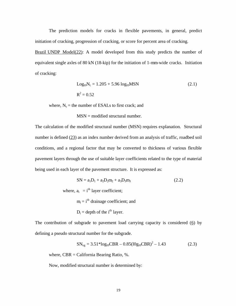
The prediction models for cracks in flexible pavements, in general, predict
initiation of cracking, progression of cracking, or score for percent area of cracking.
Brazil UNDP Model(22): A model developed from this study predicts the number of
equivalent single axles of 80 kN (18-kip) for the initiation of 1-mm-wide cracks. Initiation
of cracking:
Log10Nc = 1.205 + 5.96 log10MSN (2.1)
R2 = 0.52
where, Nc = the number of ESALs to first crack; and
MSN = modified structural number.
The calculation of the modified structural number (MSN) requires explanation. Structural
number is defined (23) as an index number derived from an analysis of traffic, roadbed soil
conditions, and a regional factor that may be converted to thickness of various flexible
pavement layers through the use of suitable layer coefficients related to the type of material
being used in each layer of the pavement structure. It is expressed as:
SN = a1D1 + a2D2m2 + a3D3m3 (2.2)
where, ai = ith layer coefficient;
mi = ith drainage coefficient; and
Di = depth of the ith layer.
The contribution of subgrade to pavement load carrying capacity is considered (6) by
defining a pseudo structural number for the subgrade.
SNsg = 3.51*log10CBR – 0.85(l0g10CBR)2 – 1.43 (2.3)
where, CBR = California Bearing Ratio, %.
Now, modified structural number is determined by:

20
MSN = SN + Snsg
The progression of cracking is expressed in percentage area:
CR = -18.53 + 0.0458*B*LN + 0.000501*B*AGE*LN (2.4)
R2 = 0.64
where, CR = amount of cracking, in percentage area;
AGE = age of the pavement, years;
B = mean surface deflection by Benkelman beam, mm; and
LN = logarithm to base 10 of the number of cumulative equivalent
axles.
The Brazil study was extended and data from other studies were combined to develop the
World Bank Model described below.
HDM III Model (World Bank): Developed from a comprehensive, factorially designed
database of in-service pavements, the HDM III (6) includes models for cracking, rutting,
roughness, etc. The cracking models are developed for various types of surfaces of
flexible pavements. Models are described here for original asphalt concrete and asphalt
overlays for estimating the expected time or traffic for initiation of cracking:
Asphalt concrete original pavements:
TyCR2 = 4.21 exp(0.139 MSN – 17.1 YE4/MSN2) (2.5)
TECR2 = 0.0342 EHM-2.86 e -0.198 EY (2.6)
where, TyCR2 = expected (mean) age of surfacing at initiation of
narrow cracking, years;
TECR2 = expected (mean) cumulative traffic at initiation of narrow
cracking, million ESALs;

21
MSN = modified structural number;
YE4 = annual traffic loading, million ESALs/lane/year;
EHM = maximum tensile strain in surfacing, 10-3; and
EY = 1/(EHM4 1000 YE4), provided that EY<=6.
RTIM2 MODEL (6): The model developed from the Transportation and Road Research
Laboratory (TRRL) road costs study in Kenya combines cracking initiation and
progression in one relationship expressed in terms of cracking plus patching, as follows:
For MSN<4.0, C+P>=0:
(C+P) = 21600 NES MSN-MSN (2.7)
where, (C+P) = sum of areas of cracking and patching (m2/km/lane);
MSN = modified structural number; and
NEs = cumulative traffic loadings since latest resurfacing (million
ESALs);
This model in the incremental form is expressed for cracking progression as
?(C+P) = 21600 MSN-MSN ? NEs (2.8)
The occurrence of crack initiation is expressed as:
NCA = max{[4/MSN – 1][MSN(1+MSN)]/72;0} (2.9)
where NCA = cumulative ESALs applied during the period before crack
initiation (million ESALs)
Texas Flexible Pavement Design System Model: The basic model utilized, a sigmoid
curve, is a modification of the AASHO (American Association of State Highway Officials)
Road Test damage function. The sigmoid, or S-shaped, curve is expected to capture the

22
long-term behavior of pavements (24). The assumed form of the model for alligator
cracking is:
a = exp (-?/N)ß (2.10)
where, a = decimal score for percent area of alligator cracking;
? = [-0.97 + 0.039(T) + 0.0034(TI) + 0.018(d) – 0.0046(LL)
+ 0.0056(PI) + 0.0066(FTC)]*106;
ß = 0.14 (LL)1.29 (PI)-1.01 (FTC)0.21 (DMD)-0.39;
T = mean average monthly temperature - 500F;
TI = Thornthwaite index + 50;
d = thickness of base course layer;
LL = subgrade liquid limit in percent;
PI = plasticity index of the subgrade soil, in percent;
FTC = number of annual freeze-thaw cycles;
DMD = maximum dynaflect deflection; and
N = the number of 18-kip equivalent single axle loads.
Similar models are developed for longitudinal and transverse cracking.
Rauhut, et al.(25,26) previously described the sigmoid form and proposed a
relation to transform damage index (DI, a damage function) to percentage of area cracking
(AC) as follows:
AC = 0.19 ?3.96 DI (2.11)
In summary, the important explanatory variables for cracking employed in these
studies are cumulative ESAL, age, and structural number. Other variables used for

23
prediction of cracking include surface deflection, subgrade characteristics, and
environmental characteristics.
2.2.2.1.2 Models for Prediction of Rutting: Rutting, caused by repeated application of
traffic loading, may result from the permanent deformation of all the pavement layers.
Traffic loading causes deformation when the stresses induced in the pavement materials
are sufficient to cause shear displacements within the materials. Thus single loads or a
few excessive loads or tire pressures, causing stresses that exceed the shear strengths of
the materials, can cause plastic flow, resulting in depressions under the load. Repeated
loadings at lesser load and tire pressure levels cause smaller deformations which
accumulate over time and manifest as a rut if the loadings are channelized into wheel-paths.
In modern pavement construction, rutting due to densification and deformation in the lower
layers under traffic loading is usually minor because it is taken into account in the
structural design methods, but can become significant when the pavement is weakened by
water ingress (6). Indeed, rutting develops by plastic flow in bituminous surface layers if
the bituminous materials are soft under high temperatures. Various models for prediction
of rutting are developed based on mechanistic responses, strength of pavement, age,
cumulative traffic, etc. A model based (27) on permanent strain is:
log εP = a + b logN or εP = ANb (2.12)
where, εP = permanent strain;
N = number of load repetitions;
a & b = experimentally determined factors; and
A = antilog of “a”.

24
HDM Model(6): Mean rut depth:
RDM = t0.166 MSN-0.502 COMP-2.30 NE4ERM (2.13)
R2 = 0.42, SEE = 1.71 mm, N = 2546
where, ERM = 0.0902 + 0.0384 DEF – 0.009 RH + 0.00158 MMP Acrx (2.14)
RDM = mean rut depth in both wheel paths, mm;
t = age of pavement since rehabilitation or construction, year;
MSN = modified structural number;
COMP = compaction index of flexible pavements, fraction;
NE4(t) = cumulative traffic loading at time t, million ESAL;
DEF = mean peak Benkelman beam deflection under 80 kN standard axle
load of both wheel paths, mm;
RH = rehabilitation state (=1 if pavement overlay, =0 otherwise);
MMP = mean monthly precipitation, mm per month; and
Acrx = area of indexed cracking, percent of total surfacing area.
Texas Transportation Model(24): The model form is identical to that for alligator cracking
(see Equation 2.10)
s = exp(-?/N)ß (2.15)
where, s = decimal severity score for rutting;
? = [3.24 – 4.89(DMD) + 0.083(T) – 0.030(TI)]*106;
ß = 0.39 (PI)-0.63 (DMD)0.54 (T)1.02; and
N = the number of 18-kip (80 KN) ESALs.

25
Rutting, as can be seen from the above models, is predominantly affected by traffic,
structural number, deflection, and subgrade characteristics.
2.2.2.1.3 Models for Prediction of Roughness: Roughness has an important bearing on the
performance of a pavement. Most of the roughness prediction models developed are for
flexible pavements, with some of them for unpaved roads. The models for paved roads
are briefly reviewed.
The AASHO Road Test (28) quantified the effects of pavement strength and traffic
loading on road roughness. Roughness models from the Transportation and Road Research
Laboratory (TRRL) study also show strong effects of pavement strength and traffic loading
(29).
TRRL Model:
Rt = R0 + s(S) Nt (2.16)
where, s(S) = function of modified structural number;
R0, Rt = roughness at time t=0, and at t, respectively; and
Nt = cumulative number of equivalent 80 kN standard axle loads to time t.
Arizona Model(30):
Ri = C0 + C1 + C2T2 (2.17)
where, Ri = roughness for homogeneous section (in/mile)
T = years since the treatment, and
C0, C1 and C2 = regression coefficients.
The study indicated that C2 coefficient was not significant, and hence roughness
showed a linear relationship with time.
26
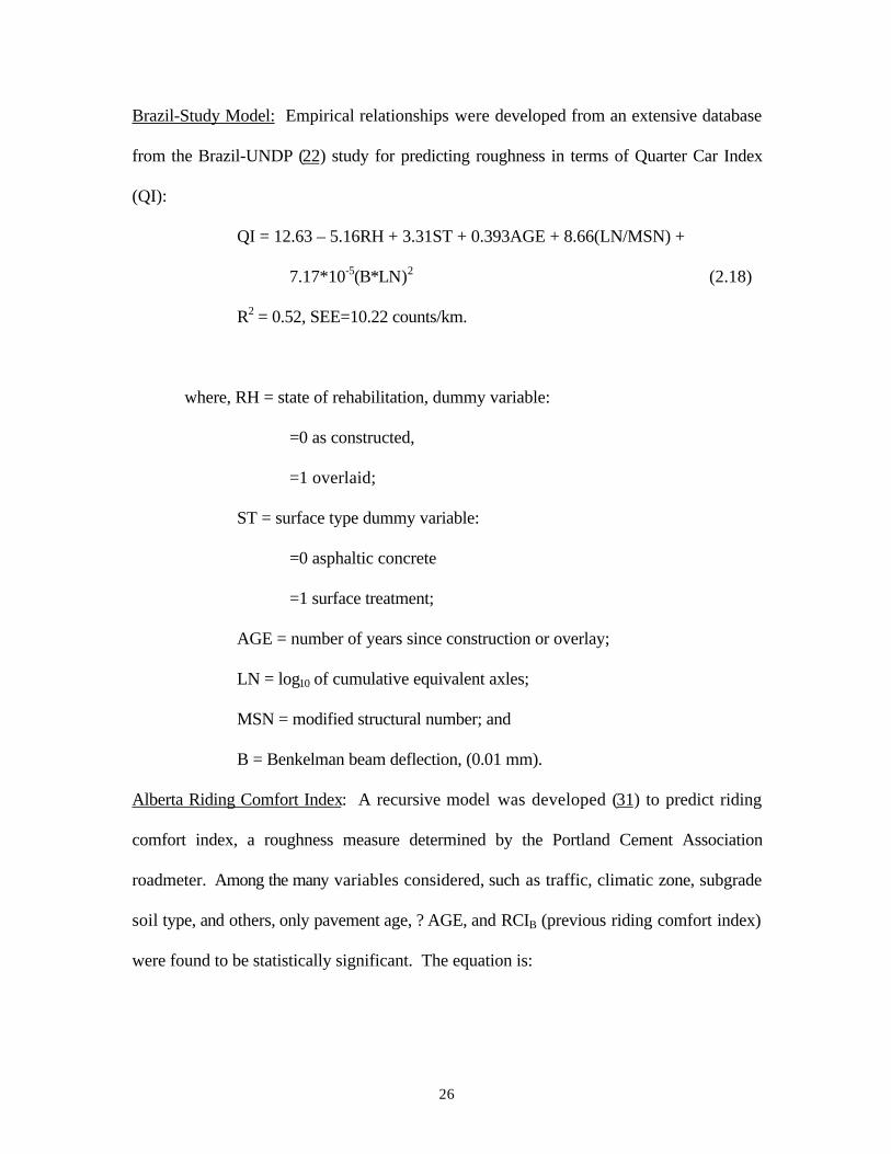
Brazil-Study Model: Empirical relationships were developed from an extensive database
from the Brazil-UNDP (22) study for predicting roughness in terms of Quarter Car Index
(QI):
QI = 12.63 – 5.16RH + 3.31ST + 0.393AGE + 8.66(LN/MSN) +
7.17*10-5(B*LN)2 (2.18)
R2 = 0.52, SEE=10.22 counts/km.
where, RH = state of rehabilitation, dummy variable:
=0 as constructed,
=1 overlaid;
ST = surface type dummy variable:
=0 asphaltic concrete
=1 surface treatment;
AGE = number of years since construction or overlay;
LN = log10 of cumulative equivalent axles;
MSN = modified structural number; and
B = Benkelman beam deflection, (0.01 mm).
Alberta Riding Comfort Index: A recursive model was developed (31) to predict riding
comfort index, a roughness measure determined by the Portland Cement Association
roadmeter. Among the many variables considered, such as traffic, climatic zone, subgrade
soil type, and others, only pavement age, ? AGE, and RCIB (previous riding comfort index)
were found to be statistically significant. The equation is:

27
RCI = -5.998 + 6.870*LOG?(RCIB) – 0.162*LOG?(AGE2 + 1)
+ 0.185*AGE – 0.084*AGE*LOG?(RCIB)
- 0.093*? AGE (2.19)
R2 = 0.84, SEE = 0.38
where, RCI = Riding Comfort Index (state of 0 to 10) at any AGE;
RCIB = previous RCI;
AGE = age in years; and
? AGE = 4 years.
Summarizing, the literature indicates that the most important variables employed in
estimating roughness are age, and traffic (cumulative ESALs).
2.2.2.2 Rigid Pavement Deterioration Models
The literature reveals that studies to develop rigid pavement deterioration models
are not as extensive as for flexible pavements. The COPES (14) study was the first
comprehensive study in this area. Separate models were developed for jointed plain
concrete and jointed reinforced concrete pavements. The distresses predicted include:
pumping, joint faulting, joint deterioration, slab cracking, and Present Serviceability Rating
(PSR). ‘National’ models (14) were developed using COPES database, compiled from six
states and other studies. The model to predict the slab cracking of jointed plain concrete
pavements follows:
CRACKS = ESAL 2.755 [3092.4(1-SOILCRS)RATIO10]
+ ESAL0.5 (1.233 TRANGE2.0 RATIO2.868)
+ ESAL2.416 (0.2296FI1.53 RATIO7.31) (2.20)

28
R2 = 0.69, SEE = 176 ft/mile, N = 303
where, CRACKS = total length of cracking of all severities, ft/lane mile;
ESAL = accumulated 18-kip equivalent single-axle loads, millions;
SOILCRS = 0, if subgrade is fine-grained; 1, if subgrade is coarse grained;
RATIO = Westergaard’s edge stress/modulus of rupture (stress computed
under a 9- kip wheel load);
FI = freezing index; and
TRANGE = difference between average maximum temperature in July and
average minimum temperature in January.
A different model for jointed reinforced concrete was developed:
CRACKS = ESAL0.897 [7130.0 JTSPACE / (ASTEEL*THICK5.0)]
+ESAL0.10 (2.281 PUMP5.0)+ESAL2.16 [1.81/(BASETYP+1)]
+AGE1.3 [0.0036(FI+1)0.36] (2.21)
R2 =0.41, SEE = 280 ft/mile, n = 314
where CRACKS = total length of medium- and high-severity deteriorated
temperature and shrinkage cracks, ft/mile;
ESAL = accumulated 18-kip equivalent single-axle loads, millions;
JTSPACE = transverse joint spacing, ft;
ASTEEL = area of reinforcing steel, in2/ft width;
THICK = slab thickness, in;
PUMP = 0, if no pumping exists; 1, low severity; 2, medium severity; 3 high
severity;
BASETYP = 0, if granular base; 1, if stabilized base (cement,

29
asphalt, etc.);
AGE = time since construction, years (indicator of cycles of cold and warm
temperatures stressing reinforcing steel); and
FI = freezing index.
Texas Models for Distresses in CRCP: The Texas models (32) make use of age as the only
explanatory variable to predict distresses in continuously reinforced concrete pavements.
Developed using a database containing 20 years of historical condition survey data, the
models predict punchouts (minor and severe), patches (asphalt and Portland cement
concrete), crack spacing, loss of ride quality, and spalling. A generalized sigmoidal
function, specified by Texas Department of Transportation, is adopted for predicting the
distresses:
D = a exp(-(?es?)ß/N) (2.22)
where, D = predicted level of distress;
N = age of the pavement;
a, ß and ? = shape parameters estimated by regression;
? = a factor to adjust for traffic;
e = a factor to adjust for environment; and
s = a factor to adjust for pavement structure.
For the purpose of analysis ?, e, and s were fixed at 1.0, due to a lack of required data.
The resulting model form is the same as Equation 2.10.
Different models are used to predict minor punchouts and severe punchouts. a, ß
and ? for prediction of minor punchouts are 82.9, 1.33, and 18.6, respectively. For

30
prediction of severe punchouts the corresponding values are 35, 0.57, and 144,
respectively.
Crack spacing is the dependent variable in the crack prediction model. Separate
equations are developed for CRC pavements with siliceous river gravel aggregate, and
limestone aggregate. The values of parameters a, ß and ? for CRCP with siliceous gravel
are, respectively 34.9, 1.00, and 0.06; while those for CRCP with limestone are 19.79,
1.06, and 0.05.
The loss of smoothness is molded in this study as Normalized Serviceability Loss
(NSL):
NSL = (4.5-PSI) / 4.5 (2.23)
Where PSI is the Present Serviceability Index. NSL ranges from 0 (PSI>=4.5) to 1
(PSI=0). For example, if the PSI of a section is 3.5, then the section is assumed to have
lost 1 Serviceability Index (SI) unit of ride quality, giving an NSL of 0.22. This means that
the section has lost 22 percent of its initial smoothness.
2.2.2.3 Models for prediction of Composite Condition Index
A composite condition index indicates the overall condition of a pavement. In
general, it is a function of surface distress or roughness or both, and measures indices of
damage, condition or serviceability. Different indices are used by various agencies to
indicate the condition of pavement. Starting from the AASHO Road Test (28) when the
concept of serviceability was proposed, many models have been developed to predict the
condition index of a pavement. The Present Serviceability Index (PSI) developed from the
AASHO Road test is a function of slope variance (a measure of roughness), average rut
depth, and area of cracking and patching.

31
AASHO PSI Model: In conjunction with the AASHO Road Test, a road user definition of
pavement failure was introduced. For flexible pavements, the model for serviceability in
terms of PSI follows:
PSI = 5.03 – 1.91 log(1+SV) – 1.38 (RD)2 – 0.01 (C+P)0.5 (2.24)
where, SV = slope variance;
RD = average rut depth; and
C+P = area of cracking plus patching per 1000 ft2.
PENNDOT Performance Prediction Model: PENNDOT model (29) is developed to
estimate PSI of reinforced concrete pavements, solely as a function of pavement age. The
equation presented in a linear form is,
PSI = 4.24 – 0.0420(AGE) (2.25)
where, PSI = the mean PSI predicted for concrete pavements with joint spacing of
61.5 ft; and
AGE = the age of the pavements in years.
State of Washington Model: The Pavement Condition Rating (PCR), a measure of
pavement surface distress (ranges from 100-no distress, to 0-extensive distress), is
predicted (29) as a function of two variables—age, and ESAL or thickness of overlay
(THICK). The equations for asphalt concrete (new or reconstruction) and asphalt concrete
overlay are, respectively:
PCR = 100 - 3.08 (AGE) - 1.4*10-6 (ESAL) (2.26)
PCR = 95.1 - 4.51 (AGE) +2.69(THICK) (2.27)
Mississippi PCR Models: Pavement Condition Rating (PCR), a performance indicator
developed for MDOT (33) is a function of distresses and roughness. PCR, on a scale of 0-

32
100, is a function of age, traffic, and structural number or thickness of overlay. The
equations for flexible pavements with no overlay, those with overlay, and composite
pavements are, respectively:
PCR = 90 - a[exp(AGEb)-1] log[ESAL/MSNc] (2.28)
PCR = 90 - a[exp(AGEb-1] log[ESAL/MSNc] (2.29)
PCR = 90 - a[exp(AGE/T)b-1] log(ESAL] (2.30)
where, AGE = time in years since last construction;
ESAL = yearly 18-kip single axle load;
T = thickness of asphalt concrete surface for composite
pavements;
MSN = modified structural number; and
a,b,c = regression constants.
Uzan and Lytton Model: A model for PSI (34), similar to the one developed from the
AASHO Road test follows:
PSI = 4.436 - 1.686 log10(1+350 Var(RD)) - 0.881 RD2.5
- 0.031(C+P)0.5
(2.31)
R2 = 0.80
where, RD = average rut depth; and
C+P = area of cracking plus patching per 1000 ft2.
Here the intercept coefficient (4.436) is very close to the average value of the pavement
serviceability after construction (34).
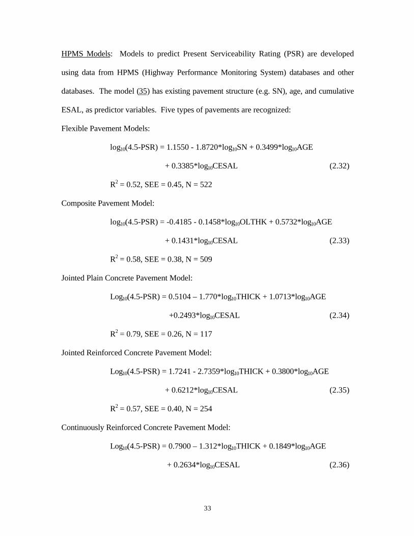
33
HPMS Models: Models to predict Present Serviceability Rating (PSR) are developed
using data from HPMS (Highway Performance Monitoring System) databases and other
databases. The model (35) has existing pavement structure (e.g. SN), age, and cumulative
ESAL, as predictor variables. Five types of pavements are recognized:
Flexible Pavement Models:
log10(4.5-PSR) = 1.1550 - 1.8720*log10SN + 0.3499*log10AGE
+ 0.3385*log10CESAL (2.32)
R2 = 0.52, SEE = 0.45, N = 522
Composite Pavement Model:
log10(4.5-PSR) = -0.4185 - 0.1458*log10OLTHK + 0.5732*log10AGE
+ 0.1431*log10CESAL (2.33)
R2 = 0.58, SEE = 0.38, N = 509
Jointed Plain Concrete Pavement Model:
Log10(4.5-PSR) = 0.5104 – 1.770*log10THICK + 1.0713*log10AGE
+0.2493*log10CESAL (2.34)
R2 = 0.79, SEE = 0.26, N = 117
Jointed Reinforced Concrete Pavement Model:
Log10(4.5-PSR) = 1.7241 - 2.7359*log10THICK + 0.3800*log10AGE
+ 0.6212*log10CESAL (2.35)
R2 = 0.57, SEE = 0.40, N = 254
Continuously Reinforced Concrete Pavement Model:
Log10(4.5-PSR) = 0.7900 – 1.312*log10THICK + 0.1849*log10AGE
+ 0.2634*log10CESAL (2.36)

34
R2 = 0.37, SEE = 0.31, N = 1204
where, PSRi = initial value of PSR at construction (4.5 used in the analysis);
STR = existing pavement structure as follows:
1. THICK, slab thickness for concrete pavements, inches
2. SN, structural number for flexible pavements,
3. OLTHK, total asphalt concrete overlay thickness for composite
pavements, inches.
AGE = age of pavement since construction or since major rehabilitation
(overlay), years; and
CESAL = cumulative 18-kip ESAL applied to the pavement (in the heavily
trafficked lane), millions.
Damage Index Model: The Texas Transportation Department employs a sigmoidal (S-
shaped) curve, a shape that appears to reproduce long term pavement performance data
(24), in modeling. Note this equation form is analogous to Equation 10.
g = exp-(?/N)ß (2.37)
where, g = damage = (Pi - P)/(Pi - Pf);
? = a constant which equals the number of 18-kip equivalent single axle
loads when g=1;
ß = a power which dictates the curvature of the damage function;
Pi = initial serviceability index;
P = present serviceability index; and
Pf = asymptote serviceability index.

35
South Carolina and Tennessee Models: Both agencies use identical form, with different
model coefficients (36):
PSI = PSI0 – exp(a-b*ct) (2.38)
where, PSI = predicted PSI;
PSI0 = PSI at age = 0 (t=0);
t = loge(1/AGE); and
a,b,c = model coefficients.
COPES Model: COPES (14) model makes use of age, traffic, distress, and environmental
factors to predict the Present Serviceability Rating (PSR). The models for jointed concrete
pavements follows:
Jointed Plain Concrete Pavement:
PSR = 4.5 - 1.486*ESAL0.1467 + 0.4963*ESAL0.265*RATIO-0.5
-0.01082*ESAL0.644*(SUMPREC0.91/AVGMT1.07)
*AGE0.525 (2.39)
R2 = 0.69, SEE = 0.25, N = 316
Jointed Reinforced Concrete Pavement:
PSR = 4.5 - ESAL0.424 - (1.88*10-3 + 14.417 RATIO3.58 + 0.0399 PUMP
+ 0.0021528 JTSPACE + 0.1146 DCRACK
+ 0.05903 REACTAG + 4.156E-5 FI + 0.00163 SUMPREC
-0.070535 BASETYP) (2.40)
where, PSR = present serviceability rating;
ESAL = accumulated 18-kip equivalent single-axle loads, millions;
RATIO = Westergaard’s edge stress/modulus of rupture;

36
SUMPREC = average annual precipitation, cm;
AVGMT = average monthly temperature, degrees C;
AGE = time since construction, years;
PUMP = 0, is none or low pumping; 1, if medium or high pumping;
JTSPACE = transverse joint spacing, ft;
DCRACK = 0, if no “D” cracking exists, 1, if “D” cracking exists;
REACTAG = 0, if no reactive aggregate exists; 1, if reactive aggregate
exists;
FI = freezing index; and
BASETYP = 0, if granular base; 1, if stabilized base (asphalt, cement,
etc.).
CRS Models for Illinois Interstate Highway System: The pavement condition indicator
used for the Illinois Interstate Highway system (37) is designated as Condition Survey
Rating System (CRS). Pavements are rated on a 1 to 9 scale on the basis of distresses
observed. The best rating of 9 is assigned to a newly constructed or resurfaced pavement.
Prediction models are developed for JRCP, CRCP, and asphalt concrete overlay of JRCP
(JROL) and CRCP (CROL). The following functional form of the model is assumed:
CRS = 9 - 2*a*THICKb.AGEc.CESALd (2.41)
The equation is expressed in the linear form by logarithmic translation and solved. The
variables are:
CRS = panel condition survey rating (1 to 9);
THICK = slab thickness for JRCP or CRCP and overlay thickness for AC
overlay;

37
AGE = years since construction or overlay;
CESAL = accumulated million ESALs in outer lane since construction or
overlay;
a,b,c,d = constants for each pavement type.
The review indicates that composite condition index models assume varying
complexity: a simple model involving only age to that involving many such factors as
roughness, traffic, structure of pavement, to name the important ones. Age is a common
explanatory variable in most of the models. The other important variables include
structural number/thickness of overlay or slab and traffic. A few models make use of
distresses for prediction of composite index.
2.2.2.4 Other Model Types
Recursive Model: Another type of model to predict distress or condition index
is the incremental, or in its purest sense, derivative model(6). It not only permits the
prediction of future deterioration as a function of time, imposed traffic, structural, and
environmental conditions, but also employs the current condition of pavement. This
property is advantageous, since the distress/condition of the pavement can be utilized as
data become available from condition surveys. The form of the model can be expressed
as:
? ( future deterioration over incremental time) = f (current condition, traffic,
strength, environment, maintenance) (2.42)
The generally slow rate of deterioration of pavements, however, means that the
changes of condition observed in empirical deterioration studies are usually small, and

38
very sensitive to measurement error. Such models also require extensive time-series data.
Therefore, incremental models are not attempted here.
All the models described above are deterministic models. However, probabilistic
models are also attempted in a few studies. Markov models and survivor curves are
examples of probabilistic models. The principles involved in the development of these
models are briefly discussed.
Markov Model: A Markov model employs a transition matrix that expresses the
probability that a group of pavements of similar age or level of traffic will move from one
state of distress or serviceability to another within a specified time period. The Markov
process describes a probable “before” and “after” condition of the pavement. The before
condition is described by probabilities that the pavement will be found in each of the
assumed finite number of states. The after condition is described in a similar manner.
With appropriate data, Markov transition matrices can be constructed for any mode of
pavement deterioration, for example, cracks, punchouts, and serviceability.
Survivor Curves: A survivor curve is a function indicating the probability of
survival of pavements with time or traffic. The probability drops off from a value of 1.0
down to zero, and expresses the percentage of pavements that remain in service after a
number of years or passes of traffic load without requiring major maintenance or
rehabilitation. The slope of the survivor curve is the probability density of survival.
Survivor curves are developed from historical data of pavements and are useful in
planning maintenance and rehabilitation alternatives on pavement networks.
Probabilistic models are not attempted in this study and, therefore, will not be
discussed further. Another relatively novel approach for formulating prediction

39
algorithms, namely Bayesian regression modeling, is briefly discussed in the ensuing
section.
2.2.3 Bayesian Regression
An emerging technique for performance modeling is to incorporate expert opinion
in the observed data. Use of expert opinion falls generally into two categories: First,
when performance data is lacking expert opinion is sought and used as a surrogate for
observations. Second, expert opinion is employed in Bayesian regression, which
explicitly allows expert judgment collected from in-house or external experts to
complement the “poor quality” data for model building. Bayesian statistics were
developed specifically to cope with small and noisy sample data by providing a structured
way to introduce prior information into the regression analysis. Given certain constrained
assumptions, Bayesian regression develops a statistically optimal posterior multivariate
regression model based on a defined prior and field models (38).
In summary, the survey of literature indicates that many different types of regression
models are developed for the prediction of pavement distresses. They include
disaggregate models for prediction of cracks, rutting, punchouts, etc. Aggregate models,
encompassing pavement condition index/rating, are reviewed as well. Finally, Bayesian
regression analysis, which includes a detailed analysis of the prior, a classical regression
of the data, is included in this chapter. Prior to attempting the models, a brief discussion of
the database employed is presented.

40
CHAPTER 3
PMS DATABASE AND DATA FOR MODELING
3.1 INTRODUCTION
A comprehensive database is a major component/module of a pavement
management system, which serves as the basis of analyses for maintenance work programs
including prediction models. The MDOT PMS database comprises the information on the
network, with data on more than 12,000 two-lane miles.
For the purpose of collecting data, the road network is partitioned into
‘homogeneous sections’. A homogeneous section can be defined (14) as a section of
pavement that has along its length uniform characteristics, for example, structural design,
joint and reinforcement design, number of lanes, subgrade condition, construction (by the
same contract), age since opening for service, pavement materials, proportion of truck
traffic, and maintenance applied. An identification code (SECIDNUM-section
identification number) is adopted to describe each homogeneous section. It is a unique
combination of the following attributes: route number, county number, direction of survey
(N, S, E, or W), and beginning accumulated log mile. For each homogeneous section the
following classes of data are available in MDOT-PMS:
• inventory
• geometry
• construction
• history including maintenance
• traffic
• condition

41
The database is the central feature of a pavement management system as seen in Figure 1.1,
and forms a foundation for a successful PMS.
These diverse items of information are needed for fully describing a pavement
section, conducting various analyses related to PMS, and establishing links between
different modules of the PMS. Easy accessibility is also paramount, for which it is
necessary to utilize a versatile database. FOXPRO software is adopted by MDOT-PMS.
3.2 DESCRIPTION OF DATABASE
For ease of access, handling, and storage, the basic pavement data is stored in five
main databases. The database names and brief descriptions follow:
TESTDATA.DBF: Describing the inventory data, which are the physical features
of the pavement sections, this database includes the route number, name of the county in
which it is located, direction of travel, beginning accumulated log mile, ending
accumulated log mile, length of the section, type of pavement surface, classification of road
according to HPMS functional class, number of lanes, and width of lanes.
TESTORGM.DBF: The details of pavement construction are stored in this
database. Included in the database are depth of each layer, type of material used in each
layer, subgrade type, and year of construction, among others.
OVERLAY.DBF: Historic data of maintenance data is stored here, which includes
the year of maintenance, various details of type of maintenance, and overlay, if any. This
chronological data is necessary to take into account the effect of maintenance actions,
improvement in conditions due to overlay, etc.
TRAFFIC.DBF: Traffic database contains the details of traffic for each section,
such as average daily traffic (ADT), percentage of trucks in the traffic mix, and traffic

42
growth rate.
RATING.DBF: Included in this database are electronic data such as rutting, IRI
and faulting, and the PCR values calculated from the condition data. Also included are the
percentage lengths of each section with low, medium, and high severity levels of rutting as
well as 85th percentile rutting.
Environmental conditions are considered to be uniform throughout Mississippi.
Consequently, environmental data is not collected.
Apart from the data stored in the above-mentioned basic databases, condition data
which is voluminous in nature is stored in many other database files. Storing them in
different database files yields many advantages such as ease of identification, management,
analysis, and storage. Physical distresses form the main condition data. The other
condition data collected are roughness and rutting (in the case of asphalt surfaced
pavements). A brief description of physical distresses, roughness, and rutting are included.
Physical Distresses: Physical distresses, collected as a part of condition data,
appear in pavements over a period of time, due to different mechanisms. The SHRP-LTPP
Distress Identification Manual (10) describes the distresses which occur in each pavement
type. It recognizes 15 distress types for asphalt surfaced pavements, 16 for jointed
concrete pavements, and 15 for continuously reinforced concrete pavements. These
distresses are listed in Table 3.1.
For the purpose of data collection, each highway is partitioned into homogeneous
sections. A ‘video inspection vehicle’ is used in collecting distress data. Instruments for
measuring roughness and rutting are mounted on the same vehicle along with five high
resolution electronic color cameras for the distress survey. Video-photographs of the

43
pavement surface are taken with the vehicle moving at normal highway speeds. These
video-photographs are projected onto a computer-screen in the office and distress type,
severity, and extent are manually recorded using SHRP-LTPP distress identification
manual (10). To suit the conditions of Mississippi, MDOT has made minor changes in
describing the severity levels of some distresses as documented in reference (11).
Though the distress survey covers 100% of the homogeneous section, only two
samples of 500 feet per mile are examined in detail for distresses. In the case of sections
that are less than ½ a mile in length, the entire section is evaluated.
Roughness: The roughness data is collected using South Dakota type profilometer
(11). It consists of a linear accelerometer and a non-contact laser device mounted on a
standard van and controlled by an on-board microcomputer measuring roughness at normal
highway speeds. Profilometer measurements taken every 10 inches are compiled, and the
IRI in m/km for the entire length of each homogeneous section is provided as output.
Rutting: Rutting, collected as a part of the condition data, is the longitudinal
depression in the wheel paths. It is measured by a rut bar with three laser sensors. The
software records the following severity levels as proposed for rutting by MDOT:
Low severity > 6.4mm (1/4 inch)<= 12.8mm (½ inch)
Moderate severity > 12.8 (½ inch)<= 25.4mm (1 inch)
High severity > 25.4mm (1 inch)
Employing the above-mentioned severity levels, the percentage of length of the section in
each category is recorded.
Table 3.1. Distresses in Different Types of Pavements (Adapted from SHRPLTPP(10))

44
Asphalt ConcreteSurfaced Pavement
distress types
Jointed ConcretePavement distress
types
ContinuouslyReinforced Concrete
Pavementdistress types
Alligator Cracking Corner Breaks Durability Cracking
Block Cracking Durability Cracking Longitudinal Cracking
Edge Cracking Longitudinal Cracking Transverse Cracking
Longitudinal Cracking Transverse Cracking Map Cracking and Scaling
Reflection Cracking Joint Seal Damage Polished Aggregate
Transverse Cracking Spalling of LongitudinalJoints
Popouts
Patch/Patch Deterioration Spalling of TransverseJoints
Blowups
Potholes Map Cracking and Scaling Water Bleeding and Pumping
Rutting Polished Aggregate Lane-to-Shoulder Dropoff
Shoving Popouts Lane-to-Shoulder Separation
Bleeding Blowups Patch/Patch Deterioration
Polished Aggregate Faulting Punchouts
Raveling Lane-to-Shoulder Dropoff
Lane-to-Shoulder Dropoff Lane-to-Shoulder Separation
Water Bleeding and Pumping Patch/Patch Deterioration
Water Bleeding and Pumping
Composite Condition Index: Based on the physical distresses, rutting, faulting, and
roughness data, a composite condition index called Pavement Condition Rating is
calculated and stored in the database. Pavement Condition Rating (PCR) (11) is a rater’s
assessment on a scale of 0 to 100, of the serviceability of a pavement with respect to
quality of ride, surface defects, pavement deformation, cracking distress and maintenance
patches. PCR, as used by MDOT, is an objective statistic determined by combining ride

45
quality and distress manifestations. The ride quality or roughness rating is obtained from
road roughness measurements, while the distress rating employs severity, extent, and type
of distress. Deduct values, much like weighting factors, are introduced to signify the
magnitude of the effect that each particular distress type, severity, and extent combination
has on pavement condition. Continuous deduct point curves/equations are developed (12)
for each distress type. Finally, the roughness rating and distress rating are combined to
yield PCR using the formula:
PCR = 100((12-IRI)/12))a ((DPmax – DP)/DPmax))b (3.1)
where, IRI = road roughness, m/km;
DPmax = probable maximum deduct points with 205, 230, 185, and 145,
respectively for flexible, composite, jointed, and continuously
reinforced concrete pavements;
DP = total deduct points for a pavement section;
a = 0.9567 for flexible, jointed concrete, and continuously reinforced concrete
pavements; and 1.11 for composite pavements; and
b = 1.4857 for flexible, jointed concrete, and continuously reinforced concrete
pavements; and 1.5429 for composite pavements.
The distress attributes from a maintenance point of view, and the factors affecting
those attributes are identified from among the various available details of a pavement in the
database. Selected from this voluminous database are the required dependent (response)
and independent (explanatory) variables required for performance modeling. For
performance modeling, a pavement family approach is employed in this study.
3.3 PAVEMENT FAMILY APPROACH

46
The behavior of different types of pavements or even individual pavements within a
given type is different. This would entail developing a model for each pavement
unit, otherwise known as site-specific models. Time series data over a long period would
be needed for site-specific models. By necessity, therefore, a ‘pavement family’ approach
is adopted in this study, wherein pavements with similar surface characteristics and/or
deterioration are grouped together into ‘families’ or groups (13,39,41). Grouping
pavements into families differs from agency to agency. In consultation with the MDOT
personnel, the pavement sections in the statewide network are grouped into the following
families or groups:
• original flexible pavements
• overlaid flexible pavements
• composite pavements
• jointed concrete pavements
• continuously reinforced concrete pavements.
A brief description of each of these groups with special reference to the predominant
distresses is presented.
Original Flexible Pavements: These are the flexible pavements that are in their
first performance period. The development of distresses in these pavements, therefore, is
not influenced by the pre-existing cracks.
Overlaid Flexible Pavements: Rehabilitated flexible pavements are those that are
overlaid at least once. They form a different group owing to factors which affect the
development of distresses. With one or more layers having undergone
deterioration/cracking, they become active in reflecting these distresses in the overlaid

47
layer unless special provisions are made to arrest the development. Also, if the overlay is
not adequately bonded to the original surface, the tendency to develop low temperature
cracks would be greater. Another difference lies in the fact that the original pavement
structure may have undergone substantial rutting during its “lifetime,” therefore, the overlay
would be susceptible to further rutting.
Composite Pavements: These pavements possess characteristics derived from both
flexible and rigid pavements, because they are rigid pavements with asphalt overlay. The
structural capacity realized is due to load dispersion in the asphaltic overlay and slab
action of the concrete slab. Some of the distresses are unique to this kind of pavement, for
example, joint reflection cracking.
Jointed Concrete Pavements: These consist of concrete slabs typically 15 to 60
feet long. Because of the joints, shrinkage related cracks are minimal. But joint-related
distresses are to be reckoned with in these pavements.
Continuously Reinforced Concrete Pavements: Continuously reinforced concrete
pavements consist of slabs typically hundreds of feet long. They are provided with
reinforcement to hold tight the cracks that develop. Thus, cracks are allowed to develop,
but are kept intact. Punchout is a distress in this type of pavement. Because of fewer joints
per unit length, the rate of increase in roughness is generally lower than that of jointed
concrete pavements.
Once the pavement families are identified and the sections grouped accordingly, the
data for homogeneous PMS sections are compiled. A distinction was made between
response and explanatory variables when compiling the data.
3.4 RESPONSE VARIABLES

48
The response variables identified in Chapter 1 are extracted from the PMS
database. For this purpose and other PMS analyses requirements, the data from the
condition survey is summarized to yield distress type, severity, and extent. The condition
data analysis yields two reports, The Sample Summary Report, and The Section Summary
Report. The sample summary report summarizes the distress type, severity, and extent
found in each sample, generally 500 feet in length. The data of several samples is
extrapolated to the whole section to produce the section summary report. Mandated by the
MDOT PMS, models are required for individual distresses and distress groups as well.
Referred to as response variables, they are briefly described in the following section.
3.4.1 Response Variables in Asphalt Surfaced Pavements
Original flexible pavements, rehabilitated flexible pavements, and composite
pavements make up the asphalt-surfaced pavement group. For asphalt-surfaced pavements,
alligator cracking of medium and high severity is combined to form a single attribute. The
second distress group comprises alligator cracking of low severity and all other cracks of
all severities; i.e., block, edge, longitudinal, transverse, and reflection cracks, and is
referred to as ‘other cracks.’ Medium and high severity other cracks expressed as a
percentage of ‘other cracks’ of all severities constitute the third group. The other three
attributes, i.e., roughness, PCR, and rutting complete the list of response variables. The
calculation of the 85th percentile rutting needs some explanation. Eighty-fifth percentile
rutting is a required input in the strategy selection tree, sketched in Appendix A. Available
from the PMS database are the percent lengths of the section exhibiting low severity 6.4 to
12.8mm (0.25 to 0.5 inch), medium severity 12.8 to 25.4mm (0.5 to 1.0 inch), and high
severity >25.4mm (>1.0 inch) rutting. The 85th percentile rutting is now obtained by

49
interpolation. To illustrate, consider a section exhibiting rut depths of low, medium, and
high severity over 30% and 10% of the length. This is indicated schematically in Figure
3.1. From the diagram it is seen that 85th percentile rutting is between 12.8 and 25.4mm
(0.5 and 1 inch). By linear interpolation between 12.8 and 25.4mm (0.5 and 1.0 inch), 85th
percentile rutting is calculated to be 22.9mm (0.9 inch). Since the field data does not
include the maximum rut depth in a section, for calculation purposes, a probable maximum
rut depth of 31.8mm (1.25) inch is used in the routine used to calculate 85th percentile
rutting.
3.4.2 Response Variables in Jointed Concrete Pavements
The distresses considered in maintenance strategy selection for jointed concrete
pavements are cracks and spalling. The cracks (corner, durability, longitudinal, and
transverse) include all three severities with the extent expressed as the percentage affected
area of section (length of cracks multiplied by 1 foot). The other distress of importance,
spalling of longitudinal and transverse joints, is also expressed as percentage area
affected. Roughness, directly available in the database, is the third variable that enters the
maintenance decision tree.

50

51
3.4.3 Response Variables in Continuously Reinforced Concrete Pavements
Punchout is considered the most severe form of all the distresses in continuously
reinforced concrete pavements, expressed as the number of punchouts per km for a given
section. Longitudinal and transverse cracks constitute the other major distress class used
in the decision tree. The roughness statistic is directly available in the database.
3.5 IDENTIFICATION OF EXPLANATORY VARIABLES
Every likely variable that may affect pavement performance should be considered
initially (20). This list will typically be large. For their implementation within a PMS,
however, predictive models must utilize only those variables that can be directly measured
within acceptable cost and time constraints (6), retrieved from historical records, or
computed or estimated. A study (42) funded by SHRP-LTPP prepared a summary of
significant data elements in the SHRP National Information Management System. The lists
for asphalt surfaced and Portland cement concrete surfaced pavements are presented in
Tables 3.2 and 3.3, respectively.
For identifying variables, one suggested method (20), is to categorize the variables
under major topics that are known to affect performance, such as layer material properties,
subgrade characterization, layer geometry, climate, traffic, maintenance, and drainage. If
each of these general topics is adequately represented by one or more variables, then the
model should contain most of the important variables known to affect performance (20).

52
A preliminary list of important explanatory variables is prepared under four major
categories which affect long-term pavement behavior. Those categories include loading,
material properties, environment, and maintenance as listed in Table 3.4. This list will be
the primary source for explanatory variables.
TABLE 3.2 - Significant Data Elements in the SHRP National InformationManagement System for Pavements with Asphalt Concrete Surfaces (42)
Significant Data Elements1 Surface Thickness 16 Subsurface Drainage
2 Base/Subbase Thickness 17 Geological Classification of CoarseAggregate in HMAC
3 Surface Stiffness 18 % of Subgrade Soil Passing #200 Sieve
4 Unbound Base/Subbase Stiffness 19 Plasticity Index of Subgrade Soil
5 Bound Base/Subbase Stiffness 20 Liquid Limit of Subgrade Soil
6 Subgrade Stiffness 21 % of Subgrade Soil Finer than 0.02 mm
7 Age of Pavement 22 Type of Environment
8 Cumulative ESALs 23 Average Max. Daily Temp. By Month
9 Asphalt Viscosity 24 Average Min. Daily Temp. By Month
10 Asphalt Content 25 Thronthwaite Index
11 Percent Air Voids 26 Freeze Index
12 HMAC Aggregate Gradation 27 No. of Days Min. Temp.<32F
13 Percent Compaction of Base/Subbase 28 No. of Days Max. Temp.>90F
14 Subgrade Soil Classification 29 Number of Air Freeze Thaw Cycles
15 In-situ Moisture Content of Subgrade 30 Annual Precipitation

53
TABLE 3.3 - Significant Data Elements in the SHRP National InformationManagement System for Pavements with Portland Cement Concrete Surfaces (42)
Significant Data Elements1 PCC Surface Thickness 15 AASHTO Soil Classification of Subgrade
2 Base Thickness 16 Subgrade % Passing #200 Sieve
3 PCC Surface Thickness 17 Moisture Content of Subgrade
4 Base Stiffness 18 Joint Efficiency
5 Subgrade Stiffness 19 Thornthwaite Index
6 Age of Pavement 20 Annual Precipitation
7 Cumulative ESALs 21 Precipitation Days by Year
8 Type of Coarse Aggregate for PCC 22 Shoulder Type
9 Gradation of Coarse Aggregate for PCC 23 Subsurface Drainage Type
10 PCC Compressive Strength 24 Average Max. Daily Temp. By Month
11 AASHTO Soil Class Base/Subbase 25 Average Min. Daily Temp. By Month
12 % Compaction of Base/Subbase 26 No. of Days Min. Temp. <32F
13 Coarse Aggregate Gradation ofBase/Subbase
27 No. of Days Max. Temp. >90F
14 Fine Aggregate Gradation of Base/Subbase 28 Air Freeze-Thaw Cycles
TABLE 3.4 - Factors Affecting Pavement Condition
Load Geometry/Material Properties
Environment Maintenance
Average daily traffic
Percentage of trucks intraffic mix
Axle load
Tire pressure
Type of material ineach layer
Thickness of each layer
Type of subgrade soil
Thickness of slab (layer)
Rainfall
Temperature
Freezing Index
Type of overlay
Thickness of overlay

54
Loading is the primary factor for which the pavements are designed. Loads applied on
pavements vary in nature depending on the wheel configuration, gross vehicle weight, tire
pressure, volume of traffic, number of lanes in the direction of travel, and others. The
effect of mixed traffic loads is converted to a standard axle (18 kips) referred to as
equivalent single axle load--ESAL. ESALs for any section per day can be calculated using
the following formula:
ESAL = ADT*DF*LF*TP*ESALF (3.2)
where, ADT = average daily traffic;
DF = a directional factor expressed as a ratio that accounts for the distribution
of ESAL units by direction, e.g., east, west, north, south, etc. It is 0.5 if
there is traffic in both directions, and 1 if there is traffic in one direction
only.
LF = a lane distribution factor, expressed as a ratio, that accounts for the
distribution of traffic when two or more lanes are available in one
direction.
As suggested in AASHTO Guide (23), the following values are used: for
the number of lanes in each direction = 1, 2, 3, and 4, LF = 1, 0.9, 0.7,
and 0.625, respectively;
TP = number of trucks in total traffic expressed as a ratio; and
ESALF = Truck factor to convert axle loads to ESAL, 0.55-1.2.
To estimate the cumulative traffic, the initial traffic on a section is to be calculated. From
the known daily ESAL on a section in the nth year, initial yearly ESAL is calculated as:
ESALo = (ESALn/(1+i) n) 365 (3.3)

55
where, ESALn = ESAL in any year n;
ESALo = initial daily ESAL on the day traffic is opened on the road; and
i = rate of traffic increase expressed as a percent per year, found in
the PMS database.
Thus, ESAL is determined for use in calculating cumulative ESAL (CESAL) (43) in any
year as:
n ESALo365CESAL =S ESAL = ____________ [(1+i)n-1] (3.4)
0 loge(1+i)
Material characteristics are the next important group of factors affecting the
behavior of pavements. The structural capacity of the pavement determines largely how
safely a load can be carried by a pavement, and how long it can last in a serviceable
condition. The structural properties of different types of pavements are taken into account
by the following variables:
Flexible – modified structural number, MSN
Composite – thickness of last overlay in inches, TOPTHK
Concrete (both jointed and CRC) – slab thickness in inches, SLABTHK
In addition to the above variables, other structural attributes are considered. These
include:
SURTK - thickness of surface course, mm;
BASTK - thickness of base course, mm;
SUBTK - thickness of subbase course, mm;
STABBAS - A categorical variable for the type of base/subbase course underneath
the PCC slab. The values of variable assigned are as follows:

56
10 - if the base course is stabilized; and
1 - if the base course is not stabilized.
CEM - A categorical variable to represent whether the base course or subbase
course underneath the AC surface is cement stabilized. This distinction is
necessary because cement stabilized layers develop shrinkage cracks which
eventually reflect to the surface layer. The categorical variable takes on a
value of 10 if there is a cement stabilized layer, and 1 otherwise.
For the purpose of analysis, the environmental conditions are considered to be
uniform throughout Mississippi, and therefore, the variables listed under environmental
factors in Table 3.4 do not warrant further discussion. However, coastal regions are
expected to have unique conditions, for example, type of subgrade (mostly sandy) soil,
shallow water table, and relatively large precipitation, which are different from those
prevalent in non-coastal areas. A pavement in a coastal region is represented by a
categorical variable (COAST) of 10. For the purpose of this study the following counties
belong to the coastal region: Hancock, Harrison, Jackson, Stone, Pearl River, and George.
Another variable which takes into account the amount of exposure of a pavement to
environmental effects (e.g., number of cyclic hot and cold temperatures) is the AGE of the
pavement, represented by number of years since construction or last overlay.
The last group of variables considered in Table 3.4 is maintenance. Major
maintenance actions such as overlay are taken into account either by the modified structural
number or by thickness of overlay. But, if resurfacing is applied, the type of resurfacing
plays an important role in the future distress manifestations. Therefore, asphalt concrete
resurfacing is represented by a categorical variable (RES) of value 10, with Single

57
Bituminous Surface Treatment (SBST) and Double Bituminous Surface Treatment (DBST)
being represented by 1.
Another categorical variable which does not fall under any of the major groups in
Table 3.4 is the HPMS functional classification for highways. A categorical variable
value of 10 indicates Rural Principal Arterial, Rural Other Principal Arterial, Rural Minor
Arterial, Urban Principal Arterial–Interstate, Urban Freeway/Expressway, Urban Other
Principal Arterial and Urban Minor Arterial. For brevity this group is referred to as
HPMS, Class I. A value of 1 is used for Rural Major Collector, Rural Minor Collector
and Rural Local and referred to as HPMS, Class II. Classification of routes into these
groups is expected to reflect the differences in the strength of sections, quality of
construction, volume of traffic, and type of maintenance applied, among others.
In order to take into account the effect of interaction between the explanatory
variables, the product of the variables is considered. As an example, age alone causes
certain deterioration, and traffic alone causes certain deterioration; however, the synergism
resulting from the combined effect of age and traffic is expected to be more than the sum of
individual effects on pavement deterioration. Interaction terms account for this synergetic
effect.
Mechanistic parameters such as those indicating strength; e.g., modulus values of
materials in different layers of the pavement, are expected to be factors having significant
influence on the long-term behavior of pavements. The limitations of the database
precluded the use of these variables. Other desirable explanatory variables, particularly
for the prediction of rutting, are type of coarse aggregate used, aggregate gradation, voids

58
in mineral aggregates, properties of bitumen, etc., cannot be included in the analysis owing
to lack of data.
Summarizing, the MDOT PMS database includes a series of databases that cover
many aspects of the road network. The six modules of inventory, geometry, construction,
maintenance, traffic, and condition data make up the database. PCR calculated from the
condition data is also stored in the database. Pavements are classified into families and
distress attributes required for their maintenance evaluation are listed. Many explanatory
variables that are expected to influence the performance are elucidated. They include age,
cumulative ESAL, slab thickness, thickness of overlay, modified structural number, etc. By
necessity, categorical variables are also employed to augment the pavement attributes.
Making use of these data elements from the database, deterioration/performance models
will be developed. The details of the developmental effort comprise the next chapter.

59
CHAPTER 4
MODELING METHODOLOGY
4.1 INTRODUCTION
As the performance and distress history of a pavement depends on many variables
in extremely complex ways, pavement deterioration models are, in general, empirical or
semi-empirical. Also, purely mechanistic models predicting primary responses such as
stress, strain, or deflection are not commonly adopted (44) since these responses are not
used as ends in themselves for design, maintenance, or rehabilitation of pavements. The
prevalent method, however, is to employ time series data and develop regression models.
This study attempts regression models, and in a few cases they are augmented by Bayesian
models as well.
A database of response variables along with all the potential explanatory variables
is compiled from the PMS database. Usually a PMS database is arranged in some order.
The MDOT-PMS is arranged according to district, route number, county number, direction
of travel, and beginning accumulated log mile. To eliminate any possible bias, the
database is randomly sorted and divided into two parts, referred to as ‘in-sample’ and
‘out-of-sample’ data. The in-sample part forms the bulk of the data, about 70 percent,
which will be used in developing the regression equations.
The remaining 30 percent of the data, referred as the “out-of-sample” or “testing
data,” is used for assessing the prediction accuracy of the regression equation. The out-of-
sample data constitutes approximately 30 percent of the total to ensure that it is statistically
“large.” Random sorting is important to retain prominent features of data in the “in-
sample” as well as the “out-of-sample” data.

60
4.2 REGRESSION MODELING TECHNIQUES
The models for prediction of response variables are developed using the regression
technique. Initially, scatter plots of response variables against each of the potential
explanatory variables are obtained, determining the likely relationships between response
and explanatory variables. Also, the plots help in locating obvious errors in the data, if
any. Various model forms are attempted in an effort to develop the best possible model.
This includes trials with various techniques, such as multiple linear, model with interacting
terms, stepwise, and non-linear regression. SPSS (45) package is utilized for regression
analysis.
4.2.1 Multiple Linear Forms
Multiple linear regression is one of the most time-honored and widely used
regression techniques for the study of linear relationships among a group of measurable
variables (47). The basic assumptions are that the random errors are independent, and
normally distributed with zero mean and constant variance. Based on these assumptions,
multiple regression tries to find a set of parameters ai such that the sum of squared
residuals is minimized, also known as the least squares method. A linear model uses the
following general form of the equation:
y = a0 + a1x1 + a2x2 + ……..+ anxn (4.1)
where, y =the response variable to be predicted, such as pavement condition,
distresses, etc.
Multiple linear models are simple and yield solutions easily, as described in the literature
(47-53). It is imperative that these models be so formatted that they satisfy physically
meaningful boundary conditions.

61
HPMS Type Model: The Highway Performance Monitoring System (HPMS)
predictive models (35) for all major pavement types use an implicit linear equation. The
nonlinear form is converted to linear form by logarithmic transformation as seen in
Equations 2.32 – 2.36. Such models are used to predict a composite condition index
(namely Present Serviceability Rating, PSR) in HPMS studies.
4.2.2 Nonlinear Regression
Nonlinear regression models are those in which the parameters of the model are
nonlinearly related. In many cases nonlinear models are sought instead of linear models
because of certain advantages:
§ To retain a clear interpretation of parameters (54)
§ Uncertainty of linear approximation used for inference can be avoided
§ Parameter estimates of linear models may have undesirable properties
§ Practical, real-world problems are often nonlinear in nature
The linear models, on the other hand, are mathematically easier, with the estimators
of the parameters being obtained from an explicit mathematical expression (55). For
nonlinear regression models, one must use either an iterative procedure employing a
mathematical algorithm or an exhaustive search procedure. Also, nonlinear regression
models with more than one explanatory variable, with few exceptions, tend to be
algebraically very complicated.
Different forms of nonlinear models are considered for modeling. Though two
forms are employed in this study, only power form turned out to be relevant in this study.
4.2.2.1 Power Form
A typical power form model employs the product of explanatory variables raised to

62
some power. This type of model is adopted in HPMS (35), Illinois (37), and Virginia (21)
studies. The general form of the equation is as follows:
y = A0 + A1 X1A2 X2
A3 X3A4 (4.2)
where y the response variable, Xi are the explanatory variables, and
A0, A1, A2, A3, and A4 the parameters of the equation.
The desirable properties of the power form of the equation, shown in Figure 4.1, are listed
below:
(a) The response variable increases or decreases monotonically which represents the
real-world physical condition. The distresses increase monotonically as
represented by curves A, B, C, and PCR decreases monotonically as represented
by the curve D.
(b) The initial condition is satisfied; i.e., the curve starts with an initial value, which
can be employed to represent the zero initial distress (curve B), a fixed value of
initial roughness (curve A), or a starting value of PCR (curve D).
(c) The delay in the development of distress can be represented, e.g., alligator cracks,
or punchouts might appear after a few years as represented by the curve C.
(d) Random distresses appear initially, increase slowly and, thereafter, increase
rapidly due to wear-out, and can be represented by this form of the equation.
4.3 MODELING BY BAYESIAN REGRESSION
In some models a Bayesian regression approach was adopted augmenting the
classical regression approach for a number of reasons. Generally, the Bayesian approach
allowed the development of better models than could be possible with data alone. This

63
64
was achieved by combining, using Bayesian regression, the performance data with prior
experience and knowledge (expert opinion) that was available through the engineering staff
of MDOT.
Predictive models require a large number of observations in order to provide a
good coverage of all factors included over a reasonable reference space. Since the
performance models are fundamentally a function of time, data needs to be available over a
reasonable time span (10-20 years) for pavement being observed. One solution lies in the
use of Bayesian regression in which the data collected in the traditional manner is
supplemented with “prior” knowledge. The so-called prior knowledge may be drawn from
expert judgment, “old” data sets, or knowledge that is generally accepted in the field.
Expert judgment can also be encoded by polling experts and asking them to estimate the
value of the dependent variable for a combination of contributory/explanatory variables.
Once compiled, this information would supplement the primary database at hand. The
prior experience ensures that the resulting performance models spanned the service life of
the pavements.
Bayesian regression relies on two models, the prior model developed from expert
judgment, and the data-model from field data. The data employed was the same as that
used in classical regression. Ten experts, each with 10 to 35 years of experience,
participated in developing the prior data. Experts were briefed on the purpose of the data
explaining the causal variables chosen for predicting a response variable, say, PCR. Their
judgments (expressed in terms of numerical scores) were encoded using a full-orthogonal
matrix elicitation technique. Experts were briefed with respect to the problem and
variables in the specified model. Subsequently they were requested to complete one

65
encoding matrix for each pavement similar to the one in Figure 4.2. Each cell in the matrix
defines a pavement with a specific combination of the four explanatory variables.
Illustrated in Figure 4.2, is a matrix for the PCR of original flexible pavements, duly filled
in by one expert. Each entry reflects his experience in working with original flexible
pavements in Mississippi. Since only one equation was desired for each pavement family,
the responses of the 10 experts were pooled to give a single collective prior.
The analysis was performed using XL-BAYS Bayesian regression software, which
runs as an add-in to Microsoft Excel (38). The program sequentially analyses the prior and
the field data thereby generating the “posterior” model. For comparison purposes, it
provides a complete statistical summary for the prior model, the data model (identical to
classical regression), and the posterior model. As the Bayesian regression software is
constrained to use only linear models, Bayesian could not improve all of the prediction
models. Linear and power equations could be handled, the latter using a linearization
procedure by taking the logarithm of the variables.
In summary, chapter 4 describes modeling methodologies employed in developing
prediction equations. In essence, regression techniques form the basis of all models, with
some models augmented by expert opinion, for which Bayesian regression methodology is
employed. Chapter 5 presents the models, explaining in some detail how they were
developed. The reasonableness of these models is verified by sketching the variation of
the response variable with age and traffic volume (CESAL).

66

67
CHAPTER 5
MODELS, RESULTS, AND DISCUSSIONS
5.1 GENERAL
This chapter documents the models developed for the prediction of distress
(distress groups)/performance of each family of pavements. Specifically, the explanatory
variables for the models, the forms of the models used and their statistics are explained.
Also documented are Bayesian models for prediction as well as improvement
accomplished using the latter approach. The last section of this chapter briefly describes a
feedback analysis program.
The sequential steps involved in modeling by regression and by Bayesian are
outlined briefly:
Classical Regression:
1. A database is created which contains the response variables and all the potential
explanatory variables.
2. The database is split into “in-sample” data comprising 70 percent of the data, with
the remaining designated “out-of-sample” for model verification.
3. A form of the model is chosen, and analyzed by stepwise regression. The procedure
aids in the identification of significant explanatory variables.
4. Regression models are developed with the in-sample data.
5. The predictive capability of the models is evaluated by comparing the predictions
with the out-of-sample data.

68
Bayesian Regression:
1. Select independent variables for inclusion in the prediction model. They need to
be the same as these used in regression modeling.
2. Either by interview or by group discussion, encode the expert’s knowledge in the
form of a matrix (see Figure 4.2).
3. Using the encoding matrix, histograms are prepared to ensure that the expert
opinions are consistent and reasonable.
4. The results provided by the expert-based models (prior data) are combined with
field data using the Bayesian regression software, XL-BAYES (38).
5. The goodness-of-fit of the posterior model is judged by testing for the significance
of the regression parameters.
For each pavement family, the models developed with the in-sample data are
described for each distress/distress group with the corresponding coefficient of
determination (R2), and root mean square error (RMSE). Following this a few of the
regression models are augmented by expert opinion increasing the inference space of the
data-based model.
5.2 ORIGINAL FLEXIBLE PAVEMENT MODELS
The original flexible pavements are those that are not overlaid, and are in their first
performance period. The explanatory variables considered are age, CESAL, MSN,
classification of road according to the HPMS system, thickness of surface, and base and
subbase courses. Note that age enters in the calculation of CESAL. To evaluate whether
multicollinearity exits between the independent variables, a correlation matrix involving
the dependent variable and the independent variables was computed. A high R2 value
between any pair of independent variables was construed as an indication of

69
multicollinearity . Another method of checking multicollinearity entails conducting a
residual analysis, the details of which can be seen in references 47 and 48. The range of
response variables employed in model development is given in Table 5.1, while that for
explanatory variables is given in Table 5.2. Models developed for each distress/distress
group or performance are described.
Table 5.1 Range of Response Variables Employed in the Development of Models, OriginalFlexible Pavements
ResponseVariable
Description Range
WCAMH Weighted alligator cracking of medium and highseverity, percent
0 - 28.61
OC Other cracks, percent 0 - 99.98
OCMH Other cracks of medium and high severity, percent 0 - 86.11
RT85 85th percentile rutting, mm 0 - 23.9
IRI Roughness, m/km 0.62 - 3.21
PCR Pavement condition rating 32 - 94
Table 5.2 Range of Explanatory Variables Used in the Development of Models, Original FlexiblePavements
Range of Explanatory Variables of ModelsExplanatoryVariable
WCAMH OC OCMH RT85 IRI PCR
Age, years 0 - 49 0 - 47 0 - 57 1- 41 0 – 46 0 - 57
18-kips CESAL,millions
0 -5.66 0 - 5.17 0 - 13.24 0.01-7.08 0 - 9.29 0 - 13.24
MSN 1.71 - 8.14 1.21 - 9.67 1.21 - 9.67 1.77 -7.93
1.21 - 9.67
5.2.1 Medium and High Severity Alligator Cracking Model
Here the percentage area of medium and high severity alligator cracking is the
response variable. Efforts to predict medium and high severity alligator cracking areas
(percentage), failed to yield satisfactory prediction models. This may be due to the fact
that some of the medium severity alligator cracking is transformed into high severity

70
alligator cracking in subsequent years. In such cases, though the percentage area of these
cracks remains the same, there is an increase in severity. To take into account the severity
effect, weights are introduced for each of these severities: 0.7 for medium severity
alligator cracking, and 1.0 for high severity alligator cracking. Assigning weights equal to
or less than one ensures that the area of cracking does not exceed the actual pavement area
(100 percent). The weighted percentage alligator cracking of medium and high severity
(WCAMH) is the response variable to be predicted.
The percentages of alligator cracking for the original flexible pavements are
observed to be low. Alligator cracking, especially high severity levels, being a serious
distress is probably not allowed to spread over a large area. Another observation is that
pavements with a modified structural number greater that 5.0 exhibit zero or very low
alligator cracking.
Alligator cracks develop due to fatigue from repeated loading cycles, and are
generally confined to wheelpaths. Cumulative 18-kip ESAL is, therefore, an important
explanatory variable for the model to predict alligator cracking. Another explanatory
variable considered is the modified structural number (MSN), an indicator of overall
strength of a pavement. To account for differences in the design standards, volume of
traffic, and quality of construction, a categorical variable—classification according to
HPMS system—is considered as well.
With little success using the above explanatory variables, age of pavement is
introduced as the fourth explanatory variable. Age is expected to account for the hardening
of asphalt resulting from loss of volatiles. Aging of bituminous binder, due primarily to
oxidation, increases the stiffness of both the binder and the surfacing material over time.

71
Consequently aging strongly reduces the fatigue life of thin to medium thick surfacing, but
probably has little effect on thick bituminous layers (6).
Using thickness of various layers instead of MSN did not result in a good model.
The best possible model obtained for weighted alligator cracking of medium and high
severity is:
WCAMH = 0.6956 AGE1.3686CESAL 0.8050MSN-1.961 (5.1)
R2 = 0.43, RMSE = 0.22, N = 241
(Note: CESAL is expressed in millions in Equations 5.1 – 5.35)
The above regression model shows that WCAMH increases with age and cumulative
traffic. The higher the MSN or the strength of pavement, the lesser the alligator cracks.
To improve the data-model, expert opinion was compiled for WCAMH in the three
families of pavements: original flexible, overlaid flexible and composite. How does
expert opinion compare with the field data? With 86.3 percent of observations reporting
zero WCAMH (see Table 5.3), the data-model predictions are well below those of the
experts (see Figure 5.1). Nevertheless, combining the expert opinion (prior model) with
data-model is considered important.
The coding results provided by the ten raters were aggregated to form one prior
model which was then combined with the data model. The analysis was performed using
Bayesian regression software, XL-BAYS. Since XL-BAYS can handle only linear
models, the model form needs to be restricted to the power form, noting that power

72
Table 5.3 and Table 5.4 appear in the original document, but are missing in the files.

73
Figure 5.1 Comparison of medium and high severity alligator cracks (WCAMH) predictedby data-model, expert model, and posterior model in flexible original pavement.
0
5
10
15
20
25
0 5 10 15 20 25
Age, year
WC
AM
H,
perc
ent expert opinion
posterior model
data model

74
models could be linearized by logarithmic transformation. With this transformation the
program sequentially analyses the prior and the field data, thereby generating the posterior
model. For comparison purposes, it provides a complete statistical summary of the prior
model, the data model, and the posterior model. XL-BAYS provides a unique feature
which enables the user to obtain probability density functions for the regression
coefficients (for the data-based, expert-based and the combined models) and plot them in
one composite figure for easy comparison. Comparison of the probability density functions
of a parameter, for example, that of CESAL, is presented in Figure 5.2. The shape of the
probability density functions (pdf) indicates uncertainty associated with the model
estimates. Clear from the pdf plots in Figure 5.2 is that the data-model is influenced by the
expert opinion, resulting in a larger exponent for CESAL swinging the trend in favor of the
prior model (expert judgment). This is an intuitively expected result indicating that the
posterior (combined) model is influenced by both field data and expert judgment.
The posterior model is defined in the following equation:
WCAMH = Age0.9329CESAL0.7331MSN-0.6348 (5.2)
R2 = 0.29, RMSE = 2.03
As indicated by t-statistics, the significance of the explanatory variables in
descending order is Age, CESAL and MSN.
Comparing the data-model, Equation 5.1, and posterior model, Equation 5.2, it is
noted that predictability of the latter is diminished, as indicated by low R2 and high RMSE.
This anomalous result could be attributed to exceedingly large expert WCAMH values as
compared to MDOT data (see Figure 5.1). As will be seen again in later

75

76
sections, whenever the two sets of data are exceedingly disparate, the prediction accuracy
of posterior model would invariably suffer.
Comparison predictions graphed in Figure 5.1 clearly show that the posterior
model predicts intermediate values as it is shaped by both data-model and expert opinion.
Nonetheless, posterior model is dominated by expert opinion resulting in relatively high
WCAMH predictions, a valid argument for not recommending this model.
Sensitivity analysis of the influence of age on WCAMH for different traffic levels-
in terms of yearly ESAL (YESAL)-plotted in Figure 5.3, indicates reasonable predictions
throughout a typical life span of 20 years. Convinced that the predicted values are in the
expected range, this data model (Equation 5.1) is recommended for MDOT PMS.
5.2.2 Model for “Other Cracks” (OC)
The other cracks include low severity alligator, block, edge, longitudinal, and
transverse cracking. An overall summary of OC cracks and other cracks of medium and
high severity (OCMH) is presented in Table 5.4. Though only 2.7% of the data registers
zero, numerous sections show extremely small OC crack density, presenting some
problems in developing a satisfactory model. As in WCAMH cracks, the explanatory
variables identified to have significant influence on other cracks percentage are: AGE,
CESAL and MSN. Derived from the in-sample data is the following model:
OC = 0.8892 AGE1.2128CESAL0.6612MSN-0.4606 (5.3)
R2 = 0.44, RMSE = 6.0, N = 718
It is noteworthy that the modified structural number, a measure of load capacity of flexible
pavements, appears in the equation with a negative coefficient. The negative sign

77
Figure 5.3 Variation of medium and high severity alligator cracks (WCAMH ) with agefor a range of traffic levels. Flexible original pavement, (MSN=5). YESAL=yearly equivalent single axle loads.
0
1
2
3
4
5
6
7
0 5 10 15 20 25
Age, year
WC
AM
H,
per
cen
tYESAL=40000
YESAL=80000
YESAL=150000YESAL=200000
YESAL=250000

78
indicates that the stronger the pavement, the lesser the potential for cracking.
A sensitivity analysis is performed where the evolution of cracks is depicted for
various yearly ESAL levels (see Figure 5.4). The exponential increase of cracks with age
seems to be in agreement with the field observations in original flexible pavements. As no
expert opinion was available for OC cracks, Bayesian regression could not be attempted.
5.2.3 Model for “Other Cracks” of Medium and High Severity (OCMH)
This distress group is recognized by MDOT-PMS as a factor in the maintenance
strategy selection. As encountered with other models of cracking, numerous OCMH values
(79 percent) are zero (see Table 5.4). Power and exponential models are attempted among
the nonlinear forms. Though exponential models could yield predictions with medium and
high severity cracks attaining maximum (100 percent) asymptotically, the data structure
was not amenable to this form of equation. A power model with age and CESAL,
therefore, is adopted here.
OCMH = 1.4378E-3 AGE2.3998CESAL1.1863 (5.4)
R2 = 0.86, RMSE = 1.62, N = 790
The predicted OCMH for the out-of-sample data looked skewed owing to extreme data
spread and numerous zero values. The trend lines in Figure 5.5 depict the evaluation of
cracks for various traffic levels. As expected, the OCMH cracks develop at a rapid rate
beyond 10 years, with traffic level playing a major role in crack widening process. The
Bayesian regression model is not attempted for want of expert opinion data.

79
Figure 5.4 Variation of other cracks (OC) with age for a range of traffic levels. Flexibleoriginal pavement, (MSN=5)
Figure 5.5 Variation of medium and high severity other cracks (OCMH) with age for arange of traffic levels. Flexible original pavement.
0
20
40
60
80
100
120
0 5 10 15 20 25 30 35
Age, year
OC
, per
cent
YESAL=40000YESAL=80000YESAL=150000
YESAL=200000YESAL=250000
0
10
20
30
40
50
60
0 5 10 15 20 25 30 35
Age, year
OC
MH
, p
erce
nt
YESAL=40000
YESAL=80000
YESAL=150000YESAL=200000
YESAL=250000

80
5.2.4 Rutting Model
Rutting is primarily caused by the loading of channelized traffic in a lane.
Therefore, traffic is bound to be an explanatory variable for predicting rutting. Whether
stronger pavements should show lesser rutting has been debated. However, the ten experts
seem to be divided on this issue. Mechanistic parameters such as strength or modulus
values of the various materials could not be included as they are not available in the
database. A model developed with traffic and MSN did not provide good prediction.
Another model with thickness of surface, base and subbase courses instead of MSN did not
yield good predictions either.
The database compiled from these consecutive surveys (1991, 1993 and 1995)
resulted in the following power model, expressing RT85 in millimeters.
RT85 = 0.4917 AGE0.2852CESAL0.1441 (5.5)
R2 = 0.59, RMSE = 0.15, N = 145
This model, rightly so, shows increased rutting with age and traffic.
In order to augment the model, the data-model and the expert model are combined
employing XL-BAYS. The resulting two-term model is,
RT85 =AGE0.8307CESAL0.1929 (5.6)
R2 = 0.68, RMSE=4.4
Since the posterior model captures both field data characteristics and expert
opinion, it is not expected to give good predictions with the out-of-sample data. The data-
model, Equation 5.5, provides good predictions using the 30 percent out-of-sample data.

81
Figure 5.6 Comparison of rutting prediction using data-, expert and Bayesian models.Flexible original pavement with yearly ESAL=200,000
• Figure 5.7 Variation of International Roughness Index (IRI) with age for a range oftraffic levels. Flexible original pavement, (MSN=5).
0
10
20
30
40
50
60
0 5 10 15 20 25
Age, year
RT
85,
mm
data-modelexpert modelBayesian model
0
0.5
1
1.5
2
2.5
0 5 10 15 20 25
Age, year
IRI,
m/k
m
YESAL=40000
YESAL=80000YESAL=150000
YESAL=200000YESAL=250000

82
The comparison of RT85 prediction employing the three models resulted in Figure 5.6,
where rut increase is graphed against age for yearly traffic of 200,000 ESAL. Primarily,
owing to larger data population the posterior model is closer to the data-model than to the
expert model. That none of the structural variables appears in the model should not be
construed to mean that rutting is not influenced by pavement thickness. It simply means that
both databases do not suggest such a causal factor. Having established that the Bayesian
model predicts realistic rutting, we recommend Equation 5.6 for use in the PMS.
5.2.5 Roughness Model
The task here is twofold: first, to determine the initial value of roughness of newly
constructed roads, and second, to determine the trend of roughness progression. A study
(50) of roughness values of newly constructed asphalt surfaced pavements in various states
(Kentucky, Georgia, Iowa, and Wisconsin) indicates that an initial IRI of 0.5 m/km is
common for the pavements constructed over the last two decades. A study of the MDOT-
PMS database shows slightly different numbers, thicker pavement showing smoother
surface initially.
Another special feature of the IRI data, and, for that matter, PCR data as well, is for
the IRI to increase abruptly with low CESAL, say in the zero to 1x10⁶ CESAL interval.
Another trend appears where the IRI increased slowly in the zero to 3x10⁶ CESAL range.
The pavements in the first group belong to low volume traffic roads where the pavement
roughness increases due primarily to environmental effects. It is the age that matters in this
group of pavements since traffic causes minimal roughness. In the second group; however,
traffic volume seems to be the key factor that contributes to pavement roughness. To take
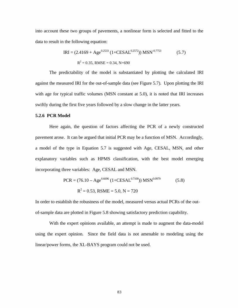
83
into account these two groups of pavements, a nonlinear form is selected and fitted to the
data to result in the following equation:
IRI = (2.4169 + Age0.2533 (1+CESAL0.2572)) MSN-0.7753 (5.7)
R2 = 0.35, RMSE = 0.34, N=690
The predictability of the model is substantiated by plotting the calculated IRI
against the measured IRI for the out-of-sample data (see Figure 5.7). Upon plotting the IRI
with age for typical traffic volumes (MSN constant at 5.0), it is noted that IRI increases
swiftly during the first five years followed by a slow change in the latter years.
5.2.6 PCR Model
Here again, the question of factors affecting the PCR of a newly constructed
pavement arose. It can be argued that initial PCR may be a function of MSN. Accordingly,
a model of the type in Equation 5.7 is suggested with Age, CESAL, MSN, and other
explanatory variables such as HPMS classification, with the best model emerging
incorporating three variables: Age, CESAL and MSN.
PCR = (76.10 – Age0.6696 (1+CESAL0.7100)) MSN0.0979 (5.8)
R2 = 0.53, RSME = 5.0, N = 720
In order to establish the robustness of the model, measured versus actual PCRs of the out-
of-sample data are plotted in Figure 5.8 showing satisfactory prediction capability.
With the expert opinions available, an attempt is made to augment the data-model
using the expert opinion. Since the field data is not amenable to modeling using the
linear/power forms, the XL-BAYS program could not be used.

84
0
Figure 5.8 Comparison of measured and predicted Pavement Condition Ratingusing original flexible pavement out-of-sample data.
40
50
60
70
80
90
100
40 50 60 70 80 90 100
Measured PCR
Pre
dict
ed P
CR

85
Figure 5.9 Comparison of Pavement Condition Rating (PCR) estimated by experts and predicted by data-models. YearlyESAL 200,000
10
20
30
40
50
60
70
80
90
100
0 5 10 15 20 25
Age, year
PC
R
Org-Flex,data
Overlaid,data
Composite,data
Org-Flex,expert
Overlaid,expert
Composite,expert

86
A comparison of the data-model and the expert opinion model, however, is taken up
for which expert opinion model similar to Equation 5.8 is derived. The expert model matches
the data model for the first eight years, beyond which, however, the experts believe the PCR
drops at a faster pace (see Figure 5.9). Recognizing that steep PCR drop is inconsistent with
the field observations, the data-model in Equation 5.8, is recommended for PMS use.
5.3 OVERLAID FLEXIBLE PAVEMENT MODELS
Overlaid flexible pavements are flexible pavements that are overlaid at least once and
form a different pavement family requiring separate models. The response variables used and
their ranges are shown in Table 5.5, while those of explanatory variables are in Table 5.6.
5.3.1 Medium and High Severity Alligator Cracking Model
In addition to the three response variables declared in the alligator crack model for
original asphalt pavements, one additional variable, surface type, was found significant. The
model equation is:
WCAMH = 0.977E-1 AGE1.8548(1+CESAL0.5336)MSN-1.9370 RES0.1618 (5.9)
R2 = 0.48, RMSE = 0.32, N = 4353
Table 5.5 Range of Response Variables Employed in the Development of Models,Overlaid Flexible Pavements
ResponseVariable
Description Range
WCAMH Weighted alligator cracking of mediumand high severity, percent
0 – 13.10
OC Other cracks, percent 0 – 89.6
OCMH Other cracks of medium and highseverity, percent
0 – 68.80
RT85 85th percentile rutting, mm 0 – 30.2
IRI Roughness, m/km 0.45 – 9.25PCR Pavement condition rating 57 – 95

87
Figure 5.10 Comparison of measured and predicted medium and high severity alligatorcracks(WCAMH) using out-of-sample data. Overlaid flexible pavement.
0
1
2
3
4
5
6
0 1 2 3 4 5 6
Measured WCAMH, percent
Pre
dic
ted
WC
AM
H,
per
cen
t

88
The out-of-sample data is predicted with the model equation plotting the results in Figure
5.10. That the agreement is fair attests to the viability of the model. Yet another plot, relating
the variations of alligator cracks with age for typical traffic levels is shown in Figure 5.11. It
is noted that very little alligator cracking develops during the early life, say, up to 6 years.
Table 5.6 Range of Explanatory Variables Used in the Development of Models, OverlaidFlexible Pavements
Range of Explanatory Variables of ModelsExplanatoryVariable WCAMH OC OCMH RT85 IRI PCR
Age, years 0 - 49 0 – 37 0 - 26 1.00-9.00 0 - 41 0 - 32
18-kip CESAL,million
0 - 2.30 0 - 6.76 0 - 4.03 0.30-1.81 0 - 6.76 0 - 6.76
MSN 1.77-9.67 0.61 - 9.52 0.61 - 9.52 0.61-9.52 0.61-9.52
TOPTHK (mm) 3.1-304.8 3.1-254.0 3.1-304.8 3.1-254
RES (categorical) AC Surface 10DBST or SBST 1
In order to improve the validity of the model, the expert model (prior model) is now
augmented by the data-model employing XL-BAYS. The experts predicted a different trend in
that the WCAMH increase was slower in the latter years. The resulting posterior model, as in
the original flexible family, includes only three explanatory variables, AGE, CESAL, and
MSN. These were the three variables employed in compiling expert opinion. The posterior
model is,
WCAMH=AGE0.5621CESAL0.1214MSN-0.4962 (5.10)
R2 = 0.31, RMSE = 2.54
The sensitivity of WCAMH to load levels is graphed in Figure 5.12, with MSN kept
constant (4.0). Showing little sensitivity to traffic level, alligator cracks begin to appear at a

89
Figure 5.11 Variation of medium and high severity alligator cracks (WCAMH) withage for a range of traffic levels using data-model. Overlaid flexible pavement,(MSN=4, RES=10)
Figure 5.12 Variation of medium and high severity alligator cracks (WCAMH) withage for a range of traffic levels using Bayesian model. Overlaid flexiblepavement, (MSN=4).
0
1
2
3
4
5
6
7
8
9
0 5 10 15 20 25
Age, year
WC
AM
H, p
erce
nt YESAL=40000
YESAL=80000
YESAL=150000
YESAL=200000
YESAL=250000
0
1
2
3
4
5
0 5 10 15 20 25
Age, year
WC
AM
H, p
erce
nt
YESAL=40000
YESAL=80000
YESAL=150000
YESAL=200000
YESAL=250000

90
very early age, though, the maximum value reaching only 3 percent level after 20 years. For
the reason that the posterior model underpredicts WCAMH the writer recommends the data
model found in Equation 5.9.
5.3.2 Model for Other Cracks
Besides Age and CESAL, the model warranted two more explanatory variables,
namely, top thickness of the top-most overlay (TOPTHK) and the resurfacing type (RES). As
dictated by the data, the best-fit model turned out to be of the following form:
OC = 19.1244 AGE0.6167(1+CESAL0.500) TOPTHK-0.6752 RES0.2713 (5.11)
R2 = 0.32, RMSE = 10, N = 3036
Among the significant explanatory variables included in the model age, traffic as well
as RES (HMA surface) tend to increase this mode of cracking. Because of the surface texture
and flexibility perhaps, surface treatment (for example, single or double bituminous surface
treatment) inhibits cracking.
The predictability of the model is investigated employing the out-of-sample data, as
shown in Figure 5.13. Evident from the data is that the model somewhat under-predicts the
crack density, especially at crack levels above 30%. The progression of cracks with age for
various traffic volumes (TOPTHK = 50.8 mm (2 inch) and RES = 10) is graphed in Figure
5.14. It is noteworthy that the cracks begin to develop at very early ages, unlike that in the
original flexible pavements where they are delayed for a few years before they begin
spreading the pavement surface.
5.3.3 Models for Other Cracks of Medium and High Severity
An equation similar in form to that for OC cracks with the same set of five variables is
found to predict medium and high severity other cracks.
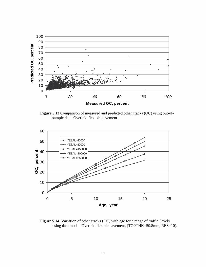
91
Figure 5.13 Comparison of measured and predicted other cracks (OC) using out-of-sample data. Overlaid flexible pavement.
Figure 5.14 Variation of other cracks (OC) with age for a range of traffic levelsusing data model. Overlaid flexible pavement, (TOPTHK=50.8mm, RES=10).
0102030405060708090
100
0 20 40 60 80 100
Measured OC, percent
Pre
dic
ted
OC
, per
cen
t
0
10
20
30
40
50
60
0 5 10 15 20 25
Age, year
OC
, p
erce
nt
YESAL=40000YESAL=80000
YESAL=150000
YESAL=200000
YESAL=250000

92
OCMH = 61.367 AGE1.4025 (1+CESAL1.6154) (5.12)
TOPTHK-2.6379 RES1.3710
R2 = 0.51, RMSE = 3.6, N = 4286
The cause-and-effect relationship of this model is identical to that for other cracks, with a
better R2, however. Note that the large exponent of RES and large negative exponent of
TOPTHK play opposite roles in Equation 5.12, indicating that cracks on HMA surface
generally overtakes those on surface treatment.
The predicted values for the out-of-sample data appear in a horizontal band (see
Figure 5.15), an indication that the model is likely to underpredict. That numerous sections
are reported to have zero cracks regardless of age and CESAL could be a reason for this
anomalous result. Figure 5.16 plots the evolution of crack with age for various traffic
volumes (TOPTHK = 50.8 mm (2 inch), HMA resurfacing). Note that beyond 10 years the
crack density increases at an exponential rate.
5.3.4 Rutting Model
Cumulative traffic and age are identified to be the significant variables for predicting
rutting. The model for 85th percentile rutting in millimeter units is:
RT85 = 5.22 AGE0.27CESAL0.0600 (5.13)
R2 = 0.47, RMSE = 4.3
Rutting is shown to increase with traffic and age, traffic playing a minor role according to the
data-model (Equation 5.13).
The expert opinion is brought to bear on the data-model employing XL-BAYS. A
power model with experts’ data is now developed and compared with the data-model noting
that the former predicts much higher rutting distress than that obtained from the data-model.

93
Figure 5.15 Comparison of measured and predicted medium and high other cracks(OCMH) using out-of -sample data. Overlaid flexible pavement.
Figure 5.16 Variation of medium and high other cracks(OCMH) with age for arange of traffic levels using data-model. Overlaid flexible pavement,(TOPTHK=50.8mm, RES=10)
0
5
10
15
20
25
30
0 5 10 15 20 25 30
Measured OCMH, percent
Pre
dic
ted
OC
MH
, per
cen
t
0
510
1520
25
3035
4045
50
0 5 10 15 20 25
Age, year
OC
MH
, per
cen
t
YESAL=40000
YESAL=80000
YESAL=150000YESAL=200000
YESAL=250000

94
This finding is not unexpected because of numerous sections (nearly 60 percent) showing
rutting less than 6.4mm (1/4 inch). With such large disparity between the prior model and the
data-model, a compromise model is sought with Bayesian regression. The model with the
same two variables is:
RT85 = 5.2498 AGE0.3583CESAL0.2524 (5.14)
R2=0.47,RMSE=4.3,N=252
The sensitivity of the posterior model is investigated by plotting the rutting
progression with age at various traffic volumes as shown in Figure 5.17. Unlike the data-
model, rutting is strongly influenced by traffic in the posterior model. With a traffic volume of
150,000 ESALs annually, a rutting of 17 mm in 15 years is judged to be reasonable;
accordingly, Equation 5.14 is recommended for MDOT’s pavement management.
5.3.5 Roughness Model
The roughness model has to satisfy the initial condition in that the initial IRI soon after
overlay should be a function of structural number, the most recent overlay thickness and a
secondary variable, the resurfacing type. The model form with five variables satisfies those
criteria.
IRI = (3.5746 + Age0.1701 (1+CESAL0.6972)) (5.15)
MSN-0.3438 TOPTHK-0.1313 RES-0.1056
R2 = 0.48, RMSE = 0.38, N = 4109
Note that the initial value of IRI is not only a function of MSN, as in the original flexible
pavement model, but also influenced by overlay thickness and surface type. As expected, a
HMA surface results in lower initial roughness than surface treatment. The thicker the

95
Figure 5.17 Variation of 85th percentile rutting (RT85) with age for a range of trafficlevels using Bayesian model. Overlaid flexible pavement.
0
5
10
15
20
25
0 5 10 15 20 25
Age, year
RT
85,
mm
YESAL=40000
YESAL=80000
YESAL=150000
YESAL=200000
YESAL=250000

96
overlay the smoother the road initially, continuing to be smooth throughout its life span. As in
the original flexible pavement model, thicker pavements inhibit road roughness.
The predictability of the model is substantiated by comparing the measured and
predicted IRI values of the out-of-sample data (see Figure 5.18). That the plotted points align
along the line of equality indicates the robustness of the model. How the model predicts road
roughness with age for various traffic levels (keeping MSN=4.0, TOPTHK=50.8mm (2 inch)
and RES=10) is graphed in Figure 5.19. The predictions are judged to be reasonable,
attesting the viability of the model.
5.3.6 PCR Model
Not only does the model need to describe the trend in PCR, it also has to predict the
initial PCR. As in the IRI model, five variables are included in the analysis to result in the
following equation:
PCR = (70.69 – Age0.6471 (1+CESAL0.7564)) MSN0.0291 TOPTHK0.0272 RES0.0198 (5.16)
R2 = 0.43, RMSE = 4.7, N = 4062
As expected, the model predicts slightly higher PCR for HMA surface. Increased
MSN, TOPTHK or HMA surface, in contrast to surface treatment, results in higher PCR in
this family of pavements.
The adequacy of the model is investigated by comparing the predicted and measured
PCR values of the out-of-sample data (see Figure 5.20). That the plotted points align along
the line of equality attests to the validity of the model. Figure 5.21 depicts how PCR

97
Figure 5.18 Comparison of measured and predicted International Roughness Index (IRI) usingout-of-sample data. Overlaid flexible pavement.
Figure 5.19 Variation of International Roughness Index (IRI) with age for a range oftraffic levels using data-model. Overlaid flexible pavement, (MSN=4,TOPTHK=50.8mm, RES=10).
0
1
2
3
4
5
0 1 2 3 4 5
Measured IRI, m/km
Pre
dic
ted
IRI,
m/k
m
0
0.5
1
1.5
2
2.5
3
3.5
0 5 10 15 20 25
Age, year
IRI,
m/k
m
YESAL=40000
YESAL=80000
YESAL=150000
YESAL=200000YESAL=250000
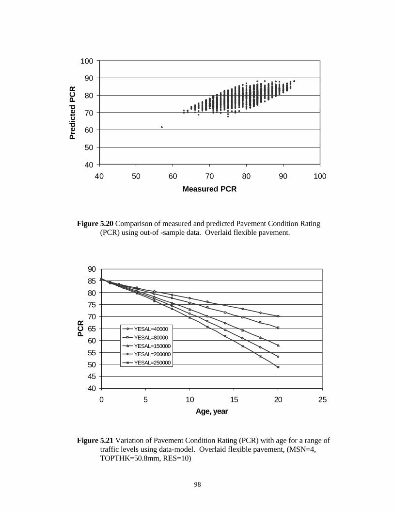
98
Figure 5.20 Comparison of measured and predicted Pavement Condition Rating(PCR) using out-of -sample data. Overlaid flexible pavement.
Figure 5.21 Variation of Pavement Condition Rating (PCR) with age for a range oftraffic levels using data-model. Overlaid flexible pavement, (MSN=4,TOPTHK=50.8mm, RES=10)
40
50
60
70
80
90
100
40 50 60 70 80 90 100
Measured PCR
Pre
dict
ed P
CR
40
4550
55
60
65
70
7580
85
90
0 5 10 15 20 25Age, year
PC
R
YESAL=40000
YESAL=80000
YESAL=150000YESAL=200000
YESAL=250000

99
decreases with age for various traffic levels, with MSN = 4.0, TOPTHK = 50.8mm (2 inch)
and HMA surface. The predicted PCRs at different ages seem to be reasonable.
With the expert opinion available, an attempt is made to augment the data-model with
the expert opinion model. For not being able to develop a linear or power model with the
field data, a necessary requirement to use XL-BAYS program, the Bayesian model could not
be pursued.
Nonetheless, it is interesting to investigate how the data model compares with the
expert opinion model. With a power model fitted for the expert opinion, the PCR trend of the
two models with age is plotted in Figure 5.9. As in the original flexible models, the trend
lines nearly coincide for the first seven-year life span, beyond which the expert predictions
substantially deviate from the data model, with the expert opinion model under-predicting
PCR, and in turn, the road’s condition. Accordingly, the data-model, Equation 5.16, is
recommended in lieu of the expert opinion model.
5.4 COMPOSITE PAVEMENT MODELS
As in overlaid flexible pavements, the primary explanatory variables considered
include age and traffic. As a measure of structural capacity, thickness of the last overlay is
considered as an explanatory variable as well. Tables 5.7 and 5.8 present the range of
response and explanatory variables, respectively.
Table 5.7 Range of Response Variables Employed in the Development of Models, CompositePavements
ResponseVariable Description Range
WCAMH Weighted alligator cracking of medium and highseverity, percent
0 – 3.0
OC Other cracks, percent 0 – 51.6OCMH Other cracks of medium and high severity, percent 0 – 14.0RT85 85th percentile rutting, mm 0 – 30.2
IRI Roughness, m/km 0.66 – 3.25PCR Pavement condition rating 56 – 94

100
Table 5.8 Range of Explanatory Variables Used in the Development of Models for CompositePavements
Range of Explanatory Variables of ModelsExplanatoryVariable
WCAMH OC OCMH RT85 IRI PCR
Age, years 0 – 22 0 - 30 0 - 28 1.00-11.00 0 - 30 0 - 29
18-kip CESAL,million
0 - 6.40 0 - 8.94 0 - 8.64 0.08-2.15 0 - 8.94 0 - 8.94
TOPTHK , mm 6.4 - 457.2 6.4 - 457.2 6.4 - 457.2 2.65-11.56 6.4 - 356.0 6.4 - 356.0
5.4.1 Medium and High Severity Alligator Cracking Model
Besides age and traffic, the data dictated one more explanatory variable for Predicting
WCAMH in composite pavements. The thickness of the most recent overlay (TOPTHK)
emerged as that variable. As can be seen in Table 5.3, numerous sections were devoid of
alligator cracking. A three-variable equation is derived as follows:
WCAMH = 0.7213E-4 Age4.0617 (1+CESAL0.5940) TOPTHK-0.5690 (5.17)
R2 = 0.53, RMSE = 0.10, N = 1143
Evaluations of WCAMH with age for various traffic volumes are graphed in Figure 5.22. The
alligator cracks increase exponentially beyond 15 years.
With expert opinion tabulated and available, it is incorporated in the data-model
employing XL-BAYS. The resulting posterior equation again includes the same three
variables as in Equation 5.17.
WCAMH = Age1.5150 CESAL0.5800 TOPTHK-0.7800 (5.18)
R2 = 0.34, RMSE = 0.98
Evolution of alligator cracking when subjected to various levels of traffic loading TPTHK
=50.8mm (2 inch), is shown in Figure 5.23. Comparing Figures 5.22 and 5.23, it is noted that
the posterior model predictions are high compared to the other two families of flexible
pavements, intuitively an unacceptable result. With reasonable WCAMH predictions as

101
Figure 5.22 Variation of Medium and high severity alligator cracks (WCAMH) withage for a range of traffic levels using data model. Composite pavement,
(TOPTHK=50.8mm).
Figure 5.23 Variation of Medium and high severity alligator cracks (WCAMH) withage for a range of traffic levels using Bayesian model. Composite pavement,
(TOPTHK=50.8mm).
0
1
2
3
4
5
6
0 5 10 15 20 25
Age, year
WC
AM
H, p
erce
nt
YESAL=40000
YESAL=80000
YESAL=150000YESAL=200000
YESAL=250000
0
2
4
6
8
10
12
0 5 10 15 20 25Age, year
WC
AM
H, p
erce
nt
YESAL=40000YESAL=80000
YESAL=150000
YESAL=200000
YESAL=250000

102
shown in Figure 5.22, the data-model, Equation 5.17 is recommended in lieu of Equation 5.18.
5.4.2 Other Cracks Model
The same three variables as for WCAMH evolved as the prominent explanatory
variables. The equation is:
OC = 15.50 Age0.5786 (1+CESAL0.5345) TOPTHK-0.4298 (5.19)
R2 = 0.43, RMSE = 5.53, N = 1292
The model predictability is illustrated by plotting the actual OC against predicted OC of the
out-of-sample data (see Figure 5.24). Note that the plotted points are aligned close to the line
of equality. Further investigation of the effect of age and traffic level on OC cracks is
undertaken, keeping TOPTHK constant at 50.8mm (2 inches), with the results graphed in
Figure 5.25. The cracks begin to appear at early age and continue to accumulate until the
pavement is totally cracked. The early distresses could be attributed to block cracking and
reflection cracking, which are caused by thermal shrinking, an age-dependent phenomenon.
This is especially true for thin overlays, typically 76.2mm (3 inches) or less. In general,
reflection cracks develop fairly early in composite pavements due to differential movement of
underlying slab. On the other hand, block cracking progresses at a steady rate in the early
period, attaining a maximum value of 100 percent in due course.
5.4.3 Models for Other Cracks of Medium and High Severity
The model for predicting other cracks of medium and high severity (OCMH
percentage) is:
OCMH = 0.8267E-2 Age2.309 (1+CESAL1.4460) TOPTHK-0.2338 (5.20)
R2 = 0.68, RMSE = 0.56, N = 1148

103
Figure 5.24 Comparison of measured and predicted other cracks (OC) usingout-of-sample data. Composite pavement.
Figure 5.25 Variation of other cracks (OC) with age for a range of trafficLevels using data model. Composite pavement, (TOPTHK=50.8mm).
0
10
20
30
40
0 10 20 30 40
Measured OC, percent
Pre
dic
ted
OC
, per
cen
t
0
10
20
30
40
50
60
0 5 10 15 20 25
Age, year
OC
, per
cen
t
YESAL=40000
YESAL=80000
YESAL=150000
YESAL=200000YESAL=250000

104
OCMH tends to increase with age and traffic volume. Thicker overlays inhibit this class of
cracks. First, the OCMH of the out-of-sample data is predicted with the equation and plotted
against the measured values, (see Figure 5.26). While the agreement is good, it is noted that
the crack density is relatively small, for instance, less than 4 percent. Second, the evolution of
OCMH at different traffic levels (at constant TOPTHK of 50.8mm) is graphed in Figure 5.27.
As these cracks form through an evolutionary process, it may be several years before they
would become noticeable. The delay period appears to be approximately 6 years, as per the
model equation.
5.4.4 Rutting Model
In addition to age and traffic volume, thickness of the most recent overlay is significant
in the prediction of pavement rutting (85th percentile):
RT85 = Age0.3690CESAL0.1300TOPTHK0.4200 (5.21)
Unlike that in the overlaid pavement the thickness of the most recent overlay appears to be a
significant variable, where rutting increases with overlay thickness.
With realistic expert opinion on pavement rutting, the data-model is incorporated in
the expert model employing XL-BAYS. The resulting posterior model has the same variables
but with somewhat different exponents:
RT85 = Age0.1217CESAL0.4973TOPTHK0.4506 (5.22)
R2 = 0.78, RMSE = 3.4
Note that the exponent of traffic is increased from 0.13 to 0.50 signifying that the posterior
model relies heavily on traffic volume to predict rutting. Importance of age is overshadowed
by CESAL in this model.
The sensitivity of the model is explored by predicting rutting with age in roads

105
Figure 5.26 Comparison of measured and predicted medium and high other cracks(OCMH) using out-of-sample data. Composite pavement.
Figure 5.27 Variation of medium and high other cracks (OCMH) with age for a rangeof traffic levels using data-model. Composite pavement, (TOPTHK=50.8mm).
01
23
4
56
7
89
0 1 2 3 4 5 6 7 8 9
Measured OCMH, percent
Pre
dic
ted
OC
MH
, per
cen
t
0
5
10
15
20
25
30
35
40
0 5 10 15 20 25
Age, year
OC
MH
, per
cen
t
YESAL=40000
YESAL=80000
YESAL=150000YESAL=200000
YESAL=250000

106
with various traffic volumes, keeping the TOPTHK constant at 50.8mm (2 inch). It is
encouraging to note that the rate of rutting declines with age. Eighty-fifth percentile rutting of
the order of 15mm in 15 years and 2.25 x 10⁶ CESAL seems reasonable (see Figure 5.28).
Accordingly, the Bayesian Model (Equation 5.22) is recommended for MDOTs’ PAP.
5.4.5 Roughness Model
The roughness model needs to satisfy an initial condition which in all likelihood
would be dependent on the overlay thickness. Only three explanatory variables appear
significant in the following model for IRI:
IRI = (3.095 + Age0.3571 (1+ CESAL0.3054)) TOPTHK-0.3235 (5.23)
R2 = 0.53, RMSE = 0.10, N = 1143
Note the initial roughness decreases with increase in overlay thickness. While IRI increases
with age and CESAL, TOPTHK promotes smoother road surface.
The predictability of the model is substantiated by comparing measured and predicted
IRI values of the out-of-sample data. The scatter of plotted points in Figure 5.29 indicates that
the model could under-predict the IRI of very rough roads. How roughness evolves with age
at various traffic levels, for a typical overlay thickness of 50.8mm (2 inches), can be seen in
Figure 5.30. With reasonable predictions recorded, the model is recommended for MDOT
pavement management system.
5.4.6 PCR Model
Again, the model has to describe the trend in PCR with time and traffic as well as
predict an initial value. A three-variable equation is found to fit these requirements:

107
Figure 5.28 Variation of 85th percentile rutting (RT85) with age for a range of trafficlevels using Bayesian model. Composite pavement, (TOPTHK=50.8mm).
0
2
4
6
8
10
12
14
16
18
20
0 5 10 15 20 25
Age, year
RT
85,
mm
YESAL=40000
YESAL=80000YESAL=150000
YESAL=200000
YESAL=250000

108
Figure 5.29 Comparison of measured and predicted roughness, IRI, using out-of-sample data. Composite pavement.
Figure 5.30 Variation of roughness, IRI, with age for a range of traffic levels usingdata-model. Composite pavement, (TOPTHK=50.8mm).
0
1
2
3
4
5
0 1 2 3 4 5
Measured IRI, m/km
Pre
dic
ted
IRI,
m/k
m
0
1
2
3
4
0 5 10 15 20 25Age, year
IRI,
m/k
m
YESAL=40000
YESAL=80000
YESAL=150000
YESAL=200000YESAL=250000

109
PCR = (56.87 – Age0.5681 (1+CESAL0.7154)) TOPTHK0.1045 (5.24)
R2 = 0.53, RMSE = 4.00, N = 1060
The thicker overlay not only results in higher initial PCR but also maintains a superior
pavement surface with time/traffic. The predictability of the model is investigated by
computing the PCR of the out-of-sample data and comparing them with the measured values
(see Figure 5.31). The agreement is satisfactory. Graphed in Figure 5.32 are trend lines
depicting PCR decrease with age at various traffic levels, holding the overlay thickness
constant at 50.8mm. Note that realistic PCRs are predicted by the model.
The quest for a Bayesian regression model is dropped as the expert opinion model
projects very low PCR values all throughout the life of the pavement (see Figure 5.9).
Neither the initial PCR of 76 nor the 15-year projected PCR of 43 for a 76mm overlay seems
reasonable. Accordingly, the data-model, Equation 5.24, is recommended for PCR
prediction.
5.5 MODELS FOR JOINTED CONCRETE PAVEMENTS
For jointed concrete pavements the following explanatory variables are considered:
age, CESAL, thickness of slab, type of base course, and classification of road according to the
HPMS system. The range of the response variables are listed in Table 5.9 and the
explanatory variables in Table 5.10.
Table 5.9 Range of Response Variables Used in the Development of Models for Jointed ConcretePavements
Response Variable Description Range
AC Cracks, percent 0 – 4.63
SP Spalling, percent 0 – 1.4
IRI Roughness, m/km 0.70 – 5.77
PCR Pavement Condition Rating 42 – 94

110
Figure 5.31 Comparison of measured and predicted Pavement Condition Rating(PCR) using out-of-sample data. Composite pavement.
Figure 5.32 Variation of Pavement Condition Rating (PCR) with age for a range oftraffic levels using data-model. Composite pavement, (TOPTHK=50.8mm).
50
60
70
80
90
100
50 60 70 80 90 100
Measured PCR
Pre
dict
ed P
CR
40
50
60
70
80
90
100
0 5 10 15 20 25Age, year
PC
R
YESAL=40000
YESAL=80000
YESAL=150000
YESAL=200000YESAL=250000

111
Table 5.10 Range of Explanatory Variables Used in the Development of Models, Jointed ConcretePavements
Range of Explanatory Variables of ModelsExplanatory Variable
AC SP IRI PCRAge, years 0 - 60 0 - 65 0 - 65 0 - 65
18-kip CESAL, million 0 - 26.83 0 - 13.5 0 - 34.3 0 - 34.3
Slab thickness, mm 127 - 330 127 - 330 127 - 330
5.5.1 Model for Cracking
Amongst the many explanatory variables considered, only three appear significant:
age, traffic, and slab thickness. The model is:
AC = 2.4118 (Age – 3)0.2465 CESAL0.5473 SLABTHK-0.3735 (5.25)
R2 = 0.28, RMSE = 0.88, N = 213
The age-shift of three years simply means that the pavement could be practically crack-free
during this period. As per the model, thicker slab, rightly so, inhibits crack density.
Understandably, cracks increase with age and traffic.
Illustrated in Figure 5.33 is a comparison of measured versus predicted cracks
employing the out-of-sample data. The plotted points are distributed over a wide band with
respect to the line of equality, a marginally acceptable result. The sensitivity of the model is
investigated in Figure 5.34, where crack density is plotted against age at various traffic
volumes, keeping the slab thickness constant at 254mm (10 inch). Two and one-half percent
cracks in 20 years for a yearly traffic volume of 250,000 ESALs appears reasonable.
5.5.2 Spalling Model
Initiated by ambient environment, joints begin to spall rapidly with traffic volume
aided by extreme temperature variations (51). With only two variables significant in

112
Figure 5.33 Comparison of measured and predicted all cracks (AC) using out-of-sample data. Jointed concrete pavement.
Figure 5.34 Variation of all cracks (AC) with age for a range of traffic levelsusing data-model. Jointed concrete pavement, (SLABTHK=254mm).
0
1
2
3
4
5
0 1 2 3 4 5
Measured AC, percent
Pre
dic
ted
AC
, p
erce
nt
0
1
2
3
4
5
6
7
0 5 10 15 20 25 30 35
Age, year
AC
, per
cen
t
YESAL=150000YESAL=200000YESAL=250000YESAL=400000
YESAL=700000

113
predicting spall, the model becomes:
SP = 0.4647*E-2 Age0.7885 CESAL0.8506 (5.26)
R2 = 0.59, RMSE = 0.13, N = 117
Judging from the nearly equal exponents for age and traffic, it may be in order to presume their
influence on spall to be nearly identical. Despite expectations that HPMS Class I pavements
might show fewer spalled joints, the data fails to reflect such a trend. Thickness of slab is not
found to be significant either.
The model predictability is evaluated by comparing the predicted spalling with the
measured, for the out-of-sample data (see Figure 5.35). In pavements with minor spalling, the
agreement is marginal, to say the least. The question whether the model can predict realistic
spalling density can be seen in Figure 5.36, where spalling with age is plotted for a range of
traffic levels. Spalling of the order of 0.5% in 30 years is considered realistic, a testament to
the validity of the model.
5.5.3 Roughness Model
A survey (50) of initial roughness of jointed concrete pavements constructed in
various states indicates that many newly constructed jointed concrete pavements exhibit an
initial roughness of 0.7m/km. A slightly higher value is indicated by MDOT data, however.
The best-fit model for IRI is:
IRI = 1.1+23.3647 Age0.2952 CESAL0.3152 SLABTHK-0.8071 (5.27)
R2 = 0.30, RMSE = 0.54, N = 205
The model indicates that roughness increases with age and traffic, but decreases with slab
thickness. Because of higher load carrying capacity thicker slabs deflect less at joints,
reducing the potential for loss of support, and in turn, reduced faulting. Pumping

114
Figure 5.35 Comparison of measured and predicted spalling (SP) using out-of-sampledata. Jointed concrete pavement.
Figure 5.36 Variation of spalling (SP) with age for a range of traffic levels using data-model. Jointed concrete pavement.
0
0.2
0.4
0.6
0.8
1
0 0.2 0.4 0.6 0.8 1
Measured SP, percent
Pre
dic
ted
SP
, per
cen
t
0
0.1
0.2
0.3
0.4
0.5
0.6
0.7
0.8
0.9
0 5 10 15 20 25 30 35
Age, year
SP
, per
cen
t
YESAL=150000YESAL=200000YESAL=250000YESAL=400000
YESAL=700000

115
tendency is also reduced with thicker slab, leading to a smoother pavement.
The out-of-sample data is employed to plot predicted versus actual IRI, resulting in
Figure 5.37. That the data points cluster along the line of equality is an indication of
acceptable predictability of the model. Another plot depicting IRI increase with age for
various traffic levels for SLABTHK = 254mm (10 inch) is presented in Figure 5.38. That the
pavement roughness increases to 2.5 m/km in 30 years at 250,000 yearly ESAL is judged to be
reasonable, providing the necessary credence to the model.
5.5.4 PCR Model
With the basic premise that the model has to satisfy both initial pavement condition
and change in PCR with time/traffic, a three-variable model is derived employing the
database:
PCR = (51.1 – 0.1603 E-3 Age1.9270 (27 + CESAL1.9000)) SLABTHK0.1000 (5.28)
R2 = 0.48, RMSE = 5.82, N = 154
The model, rightly so, predicts better pavement condition with thicker slabs.
Comparing the expert model with the data model, it becomes clear that the experts
believe that the pavement condition deteriorates faster than that predicted by the data- model.
Therefore, a compromise model is sought employing Bayesian regression. By necessity the
data-model, the expert model, and the posterior model should be in power form. In the
Bayesian formulation slab thickness is not significant:
PCR = 90 – Age0.6741 CESAL0.4924 (5.29)
R2 = 0.59, RMSE = 7.25, N = 398
The sensitivity of the model is investigated by plotting PCR with age at various traffic

116
Figure 5.37 Comparison of measured and predicted International RoughnessIndex (IRI) using out-of-sample data. Jointed concrete pavement.
Figure 5.38 Variation of International Roughness Index (IRI) with age for arange of traffic levels using data-model. Jointed concrete pavement,(SLABTHK=254mm).
0
1
2
3
4
5
0 1 2 3 4 5
Measured IRI, m/km
Pre
dic
ted
IRI,
m/k
m
0
0.5
1
1.5
2
2.5
3
3.5
0 5 10 15 20 25 30 35
Age, year
IRI,
m/k
m
YESAL=150000
YESAL=200000
YESAL=250000YESAL=400000
YESAL=700000

117
levels. It is noteworthy that both time as well as traffic affect the pavement condition with
nearly equal weight, signifying the importance of both environmental and load factors (see
Figure 5.39). Being able to predict realistic PCR values, the Bayesian model, Equation 5.29,
is recommended for MDOT PMS.
5.6 CONTINUOUSLY REINFORCED CONCRETE PAVEMENT MODELS
The explanatory variables considered for this pavement type are age, CESAL, and
slab thickness. A cursory study of the data revealed that almost all of the CRC pavement
sections (approximately 98 percent) in Mississippi have one thickness, namely 202mm (8
inches). Without data from a range of slab thickness, it could not be included as an
explanatory variable. The range of response variables is listed in Table 5.11 and the
explanatory variables in Table 5.12.
Table 5.11 Range of Response Variables Used in the Development of Models, ContinuouslyReinforced Concrete Pavements
Response Variable Description Range
AC Cracks, percent 0 – 7.2PO Punchouts, number/km 0 – 26.2IRI Roughness, m/km 1.4 – 4.1
PCR Pavement Condition Rating 60 – 90
Table 5.12 Range of Explanatory Variables Used in the Development of Models for ContinuouslyReinforced Concrete Pavements
Range of Explanatory Variables of ModelsExplanatory Variable
AC PO # IRI PCR
Age, years 0 - 36 0 - 35 0 – 33 0 - 36
18-kip CESAL, million 0 - 32.9 0 - 18.3 0 - 20.8 0 - 41.8
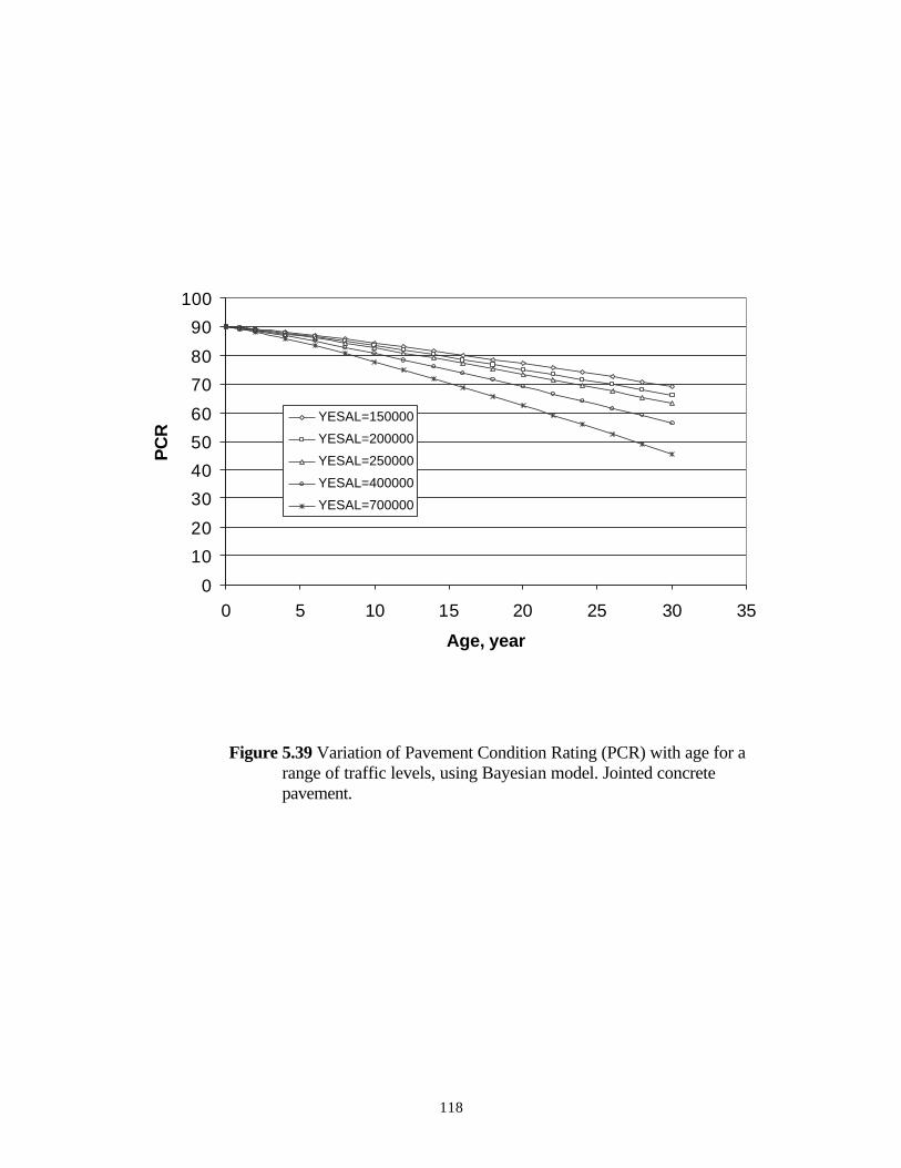
118
Figure 5.39 Variation of Pavement Condition Rating (PCR) with age for arange of traffic levels, using Bayesian model. Jointed concretepavement.
0
10
20
30
40
50
60
70
80
90
100
0 5 10 15 20 25 30 35
Age, year
PC
R
YESAL=150000
YESAL=200000
YESAL=250000
YESAL=400000
YESAL=700000

119
5.6.1 Model for Cracks
At the outset it should be remarked that low severity transverse cracks caused by
shrinkage (inherent in CRC pavements) are not counted while quantifying this distress
category. The model for medium and high severity transverse cracks (including other modes
of cracks) is:
AC = 0.1013 (Age-10)0.5837 CESAL0.6095 (5.30)
R2 = 0.44, RMSE = 0.87, N = 91
The age-shift indicates that those medium/high severity cracks would be delayed for about 10
years. Even with substantial exponents for age and traffic, the model under-predicts in
comparison to experts’ opinion. In order to strengthen the model, therefore, expert opinion is
incorporated employing Bayesian regression. The posterior model again with the two
variables is:
AC = 0.731E-1 (Age-10)0.3448 CESAL1.2377 (5.31)
R2 = 0.63, RMSE = 1.34, N = 179
The age-shift of 10 years is again retained in the model. Note the posterior model predictions
fall between the expert opinion and the data-model predictions. That is, the posterior model
reconciles the expert opinion and the data. Presented in Figure 5.40 is a graphical
representation of increase in cracks with age for a range of traffic volumes. Typically, a
prediction of 4.5 percent cracks in 30 years when sustaining an annual traffic of 400,000 is
reasonable. The Bayesian model, Equation 5.31 is the writer’s recommendation.
5.6.2 Punchout Model
A cursory examination of the data reveals that out of the sections for which

120
Figure 5.40 Variation of all cracks (AC) with age for a range of traffic levelsusing Bayesian model. Continuously reinforced concrete pavement.
Figure 5.41 Variation of punchouts (PO) with age for a range of traffic levelsusing Bayesian model. Continuously reinforced concrete pavement.
0123456789
10
0 5 10 15 20 25 30 35
Age, year
AC
, per
cen
tYESAL=150000
YESAL=200000
YESAL=250000
YESAL=400000
YESAL=700000
0
0.5
1
1.5
2
2.5
3
3.5
0 5 10 15 20 25 30 35
Age, year
PO
, per
cen
t
YESAL=150000
YESAL=200000
YESAL=250000YESAL=400000
YESAL=700000

121
punchout information is available, only 24 percent of the data had more than one punchout/km.
This low punchout count could perhaps be attributed to MDOT practice of rehabilitating them
promptly and, therefore, not interpretable in the video survey. A two-variable model is
derived for punchouts in CRC:
PO = 0.4454 * E-3 (Age –10)1.4095 CESAL1.3575 (5.32)
R2 = 0.75, RMSE = 0.13, N = 151
That punchouts begin to appear only after 10 years in service is noted from the equation. Even
with sufficiently large exponents for age and CESALs, the model under-predicts punchout, for
example 0.9 punchouts/km with 30 years of 400,000 ESALs annually.
The experts predict much higher punchout counts, as verified in the expert opinion
matrix. Encouraged by this data, Bayesian regression is employed to incorporate data-model
in the expert model. The posterior equation is:
PO = 0.33 (Age – 10)0.2571 CESAL0.4163 (5.33)
R2 = 0.48, RMSE = 0.57, N = 110
Why R2 decreased from 0.75 for the data-model to 0.48 for the posterior model warrants
explanation. That the expert opinion differed significantly from the field data could be the
major reason for this anomaly. Combining two disparate databases to develop a single model
would likely bring down the coefficient of determination from their individual coefficients.
A sensitivity study, where punchout count is plotted against age for various traffic
levels, can be seen in Figure 5.41. The resulting model is improved, in that it predicts 2.2
punchouts/km after 30 years of traffic at 400,000 ESAL yearly. The posterior model is the
choice of the writer for MDOT PMS.
5.6.3 Roughness Model

122
Newly constructed CRC pavements show initial roughness somewhat comparable to
that in jointed concrete pavements. CRC pavements in Illinois showed an average roughness
value of 1.18m/km, while those in Kansas showed 0.94m/km (50). These high values are
expected because of longer slabs which undergo warping. An IRI of 1.0m/km, therefore, is
chosen as the initial condition. The roughness model developed is:
IRI = 1 + 0.4218 Age0.1008 CESAL0.4186 (5.34)
R2 = 0.48, RMSE = 0.32, N = 146
Employing the out-of-sample data, the predictability of the model is checked plotting actual
versus predicted IRI values. The large scatter in Figure 5.42, perhaps, is an indication of the
influence of other variables, such as construction quality, that are not quantifiable at this time.
Graphs in Figure 5.43 support the view that IRI is sensitive to both age and traffic volume,
though the predominance of the latter factor cannot be overlooked. With reasonable
predictions, Equation 5.34 is recommended to MDOT.
5.6.4 PCR Model
As in all other four PCR models, the model should accommodate an initial value,
consistent with the roughness of new construction. A two-variable model is shown to forecast
pavement condition, as per the MDOT pavement data:
PCR = 91 – Age0.4085 CESAL0.5299 (5.35)
R2 = 0.65, RMSE = 2.72, N = 119
With the model generally over-predicting the pavement condition in relation to what
the experts believe, Bayesian regression is employed to combine the two. A power model
resulted from this analysis with nearly same coefficient of correlation:

123
Figure 5.42 Comparison of measured and predicted International Roughness Index(IRI) using out-of-sample data. Continuously reinforced concrete pavement.
Figure 5.43 Variation of International Roughness Index (IRI) with age for a range oftraffic levels using data-model. Continuously reinforced concrete pavement.
1
1.5
2
2.5
3
1 1.5 2 2.5 3
Measured IRI, m/km
Pre
dic
ted
IRI,
m/k
m
0
0.5
1
1.5
2
2.5
3
3.5
0 5 10 15 20 25 30 35
Age, year
IRI
YESAL=150000YESAL=200000
YESAL=250000
YESAL=400000
YESAL=700000

124
PCR = 92 – Age0.6463 CESAL0.2731 (5.36)
R2 = 0.61, RMSE = 2.75, N = 181
Judged by the t-statistic, the age variable is highly significant. It is noteworthy that the initial
PCR value of 92 corresponds to an IRI of 1m/km, exactly matching the initial value of IRI
model for CRC pavement. Graphing the Bayesian model (see Figure 5.44), we note that
pavement condition is influenced by both time and traffic. The traffic seems to have less
effect in comparison to age, for the reason CRC is structurally sound to resist traffic loads.
Judging the model to be providing reasonable predictions, the Bayesian model, Equation 5.36,
is recommended to MDOT.
5.7 PROJECT LEVEL DISTRESS/PERFORMANCE PREDICTION
For applications at the project level, corrections are to be applied to the predictions
based on the observed data. These corrections are necessary to account for the differences in
the long-term behavior of individual pavements from the predictions that are mean
deterioration trends of the pavement family.
Different procedures are suggested in the literature (52, 21) for adjustment of the
pavement family model for individual projects. The prediction relation of a pavement family
represents the average behavior of all the sections of that family. The prediction of each
project/section is accomplished by shifting its position relative to the family prediction curve.
It is assumed that the deterioration of all pavements in a family is similar. In practice,
therefore, when the observed deterioration of pavement differs from that predicted by the
model, the model should be adjusted to pass through the observed point. Predictions for
future years are then made using this augmented curve.
One method (52) is to draw a curve through the observed point parallel to the
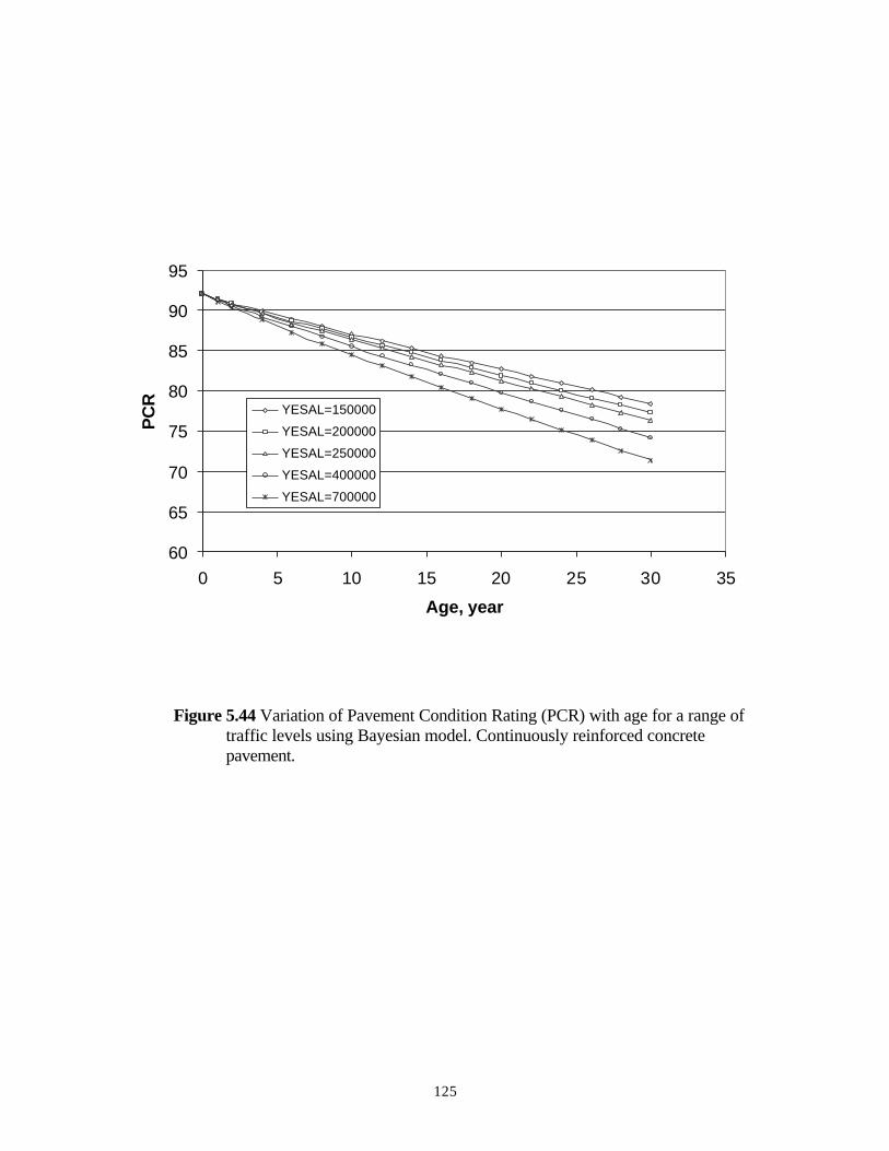
125
Figure 5.44 Variation of Pavement Condition Rating (PCR) with age for a range oftraffic levels using Bayesian model. Continuously reinforced concretepavement.
60
65
70
75
80
85
90
95
0 5 10 15 20 25 30 35
Age, year
PC
R YESAL=150000
YESAL=200000
YESAL=250000
YESAL=400000
YESAL=700000

126
developed model as shown in Figure 5.45. Since age is predominant explanatory variable,
the horizontal shift is mathematically performed by solving the model equation for the AGE
that corresponds to the observed pavement deterioration. Future predictions are made
assuming that the calculated age is the current age for the section.
A second approach (53) is to shift the curve vertically instead of horizontally as in
Figure 5.46, so that it passes through the observed point. This is done by using the actual
deterioration (D1) of the pavement and the predicted deterioration (D2) for computing an
adjustment factor defined by AF = D1/D2. Future predictions are made by multiplying the
predicted deterioration by the adjustment factor (AF). This method seems to be more
appropriate where all the involved explanatory variables are employed in prediction rather
than adjusting for only the main explanatory variable.
5.8 ENGINEERING FEEDBACK SYSTEM
The feedback module, as envisioned in the original proposal, was to ensure continual
feedback of information assessing pavement system condition, and also for
verification/substantiation of the design standards and/or specifications. Described briefly
are three submodules of the feedback system that were completed and submitted to MDOT on
31 July 1998.
1. The module that calculates the load index for the three types of pavements (flexible,
CRC and jointed concrete), as originally built. Load index is the ratio of the actual
ESAL and the design ESAL. Design ESAL is calculated using the design equations
proposed in the 1993 Revised AASHTO Guide.
2. The module that calculates the load index of overlaid flexible pavements, and

127

128
that too only for the first overlay. Again, AASHTO flexible pavement design equation
is used for this purpose. For use in the equation, the structural number of an overlaid
pavement is calculated with the revised layer coefficient of the asphalt concrete
surface, according to Transportation Management Information System (TMIS). Design
equations for other types of overlaid pavements are not readily available, therefore,
those calculations are deferred in this version of the program.
3. The third module calculates the ratio of the actual and the predicted distress of each
section of each pavement family; for example, five distresses and PCR for original
flexible, overlaid flexible, and composite pavement types. For distress predictions,
equations submitted to MDOT on 1 July 1997 were employed. Note the feedback
program was submitted to MDOT on 31 July 1998. This comparison enables us to
validate the prediction models.
The feedback module may be implemented in such a way that it can access present and
past condition data and all other inventory databases. With this information assembled
from the MDOT PMS databases, feedback analyses results can be output in the form of
reports and tables.
5.9 Summary
The models developed in the study indicate that the most important variables affecting
deterioration of all pavement types are age, cumulative traffic, and modified structural
number/slab thickness. Thickness of overlay is a significant explanatory variable in
composite pavements. HPMS functional classification and resurfacing type are other
variables in overlaid flexible pavement.

129
Age is a factor that appears in all of the models. It is a factor that represents
deterioration of pavements due to environment and/or other damage that cannot be accounted
for by traffic or other factors. A question arises as to why age plays such a dominant role in
relation to the cumulative traffic. That age can be determined very precisely is the first and
foremost reason for its significance in the model. Second, age enters into the estimation of
cumulative traffic as well as the environmental loading cycles (33). Between age and ESAL,
ESAL would be the weakest link in the cumulative traffic computation because of inclusion of
several questionable input parameters for ESAL calculation (these include sample traffic
count, growth factor, and truck factor). Between age and CESAL, the former satisfies the
assumptions required for regression modeling, discussed herein. Age is nonstochastic, that is,
its value is fixed and it is measured without error. By virtue of these facts, age would be a
better explanatory variable than CESAL.
Modified structural number, as seen in models for flexible (both original and
overlaid), does not seem to play a major part in the prediction. The first reason is that the
pavements are designed for the expected level of traffic, with heavily trafficked roads being
provided with thicker pavement sections compared to lightly trafficked ones. Therefore, the
deterioration rates of thick and thin pavements are expected to be nearly identical. The
second reason is that even nominally identical pavement sections show spatial variation in
strength properties, local deficiencies in construction, change in conditions along stretches
(for example, high water table), and other variations making the MSN data ‘noisy’. Noisy
data simply suppresses the explanatory variables’ effect on the response variable.
Cumulative traffic, expected to be the main factor causing deterioration, is also a
significant factor in all the models. Stronger pavements, in general, should undergo slower

130
deterioration, and the inclusion of a strength indicator (MSN, thickness of overlay, or
thickness of slab) in most of the models is justified.
5.9.1 Summary of Significant Variables for Each Pavement Family
The results of the sensitivity-study suggest that age is the most significant factor
affecting the deterioration of original flexible pavements. Cumulative traffic, rightly so, is the
second most significant factor for the prediction of other cracks, roughness, and PCR. The
modified structural number appears in four models except in those for medium and high
severity other cracks, and rutting.
As in the case of original flexible pavements, age and traffic play the most significant
role in distress prediction for overlaid flexible pavements. Modified structural number
and/or TOPTHK and resurfacing type are other explanatory variables in all of the models
except for WCAMH.
For composite pavements, besides age and traffic, thickness of overlay is the most
important variable affecting deterioration. In the same vein, in the models for jointed concrete
pavements, slab thickness appears in addition to age and traffic. In the case of continuously
reinforced concrete pavements, age and traffic are the only two variables significant enough to
appear in the models.

131
CHAPTER 6
SUMMARY AND CONCLUSIONS
6.1 SUMMARY
The focus of the study has been to develop deterioration/performance models for
pavements for use in pavement management analysis algorithms. The models are derived such
that they satisfy many physical and boundary conditions with known causal variables. In
contrast to many other studies cited in the literature, actual data on pavements are employed
rather than accelerated road test data. Another characteristic feature of the study is the
application of Bayesian regression employing expert opinion to augment data-models.
Deterioration models are developed for distress/distress groups employed in the
decision tree for maintenance strategy selection adopted by MDOT-PMS. The models are
derived using the in-sample data and subsequently verified using the out-of-sample data. As
deemed appropriate, Bayesian models are attempted in 14 different distresses. Only seven of
them are found to generate models superior to the corresponding data models.
6.1.1 Regression Models
Various model forms were attempted in the study but only nonlinear ones are
employed because of their prediction capability. Multiple linear models do not satisfy the
required boundary conditions, including monotonic variation (increase or decrease) of the
deterioration rates. The primary advantage of the general power form and exponential form of
the nonlinear models is that they do not rely on fixed exponents, such as squares or cubic
powers. This flexibility in the exponent immensely improves the modeling process. Lack of
distress data in severely deteriorated pavements precluded the use of exponential forms in any
of the models. Out of a total of 26 equations, 19 are regression models and the remaining 7

132
are Bayesian models. Because of the large disparity between the field data and the expert
opinion, Bayesian regression for four distresses produced models whose predictions are
suspect. In three cases - PCR models of three flexible families - the data models appeared
satisfactory, accordingly, they are preferred over Bayesian models. The models are listed in
Tables 6.1-6.5, one table for each family.
Table 6.1 - Deterioration Models for Original Flexible Pavements
DISTRESS MODELWeighted Alligator Cracking ofMedium and High Severity,percent
WCAMH = 0.6956 AGE1.3686 CESAL0.8050 MSN-1.961
Other Cracks, percent OC = 0.8892 AGE1.2128 CESAL0.6612 MSN-0.4606
Other Cracks of Medium andHigh Severity, percent
OCMH = 0.1438 E-2 AGE2.3998 CESAL1.1863
85th Percentile Rutting, mm RT = AGE0.8307 CESAL0.1929
Roughness, (IRI) m/km IRI = (2.4169+AGE0.2533(1+CESAL0.2572))MSN-0.7753
PCR PCR = (76.10-AGE0.6696 (1+CESAL0.7100))MSN0.0979
Table 6.2 – Deterioration Models for Overlaid Flexible Pavements
DISTRESS MODELWeighted Alligator Cracking ofMedium and High Severity,percent
WCAMH = 0.977E-1 AGE1.8548 (1+CESAL0.5336)MSN-1.9370
RES0.1618
Other Cracks, percent OC = 19.1244 AGE0.6167 (1+CESAL0.5000) TOPTHK-0.6752 RES0.2713
Other Cracks of Medium andHigh Severity, percent
OCMH = 61.367 AGE1.4025 (1+CESAL1.6154) TOPTHK-2.6379
RES1.3710
85th Percentile Rutting, mm RT85 = 5.2498 AGE0.3583 CESAL0.2524
Roughness, (IRI) m/km IRI = (3.5746 + AGE0.1701 (1+CESAL0.6972))MSN-0.3438
TOPTHK-0.1313 RES-0.1056
PCR PCR = (70.69-AGE0.6471 (1+CESAL0.7564))MSN0.0291 TOPTHK0.0272
RES0.0198

133
Table 6.3 – Deterioration Models for Composite Pavements
DISTRESS MODEL
Weighted AlligatorCracking of Medium andHigh Severity, percent
WCAMH = 0.7213 E-4 AGE4.0617(1+CESAL0.5940)TOPTHK-0.5690
Other Cracks, percent OC = 15.50 AGE0.5786(1+CESAL0.5345)TOPTHK-0.4298
Other Cracks of Mediumand High Severity, percent
OCMH = 0.8267 E-2 AGE2.3090(1+CESAL1.4460)TOPTHK-0.2338
85th Percentile Rutting, mm RT85 = AGE0.1217CESAL0.4973TOPTHK0.4506
Roughness, (IRI) m/km IRI = (3.095+AGE0.3571(1+CESAL0.3054))TOPTHK-0.3235
PCR PCR = (56.87-AGE0.5681(1+CESAL0.7154))TOPTHK0.1045
Table 6.4 – Deterioration Models for Jointed Concrete Pavements
DISTRESS MODELCracks, percent AC = 2.4118(AGE-3)0.2465CESAL0.5473 SLABTHK-0.3735
Spalling, percent SP = 0.4647E-2 AGE0.7885 CESAL0.8506
Roughness, (IRI) m/km IRI = 1.1 + 23.3647AGE0.2952CESAL0.3152 SLABTHK-0.8071
PCR PCR = 90.00 – AGE0.6741 CESAL0.4924
Table 6.5 – Deterioration Models for Continuously Reinforced Concrete PavementsDISTRESS MODEL
Cracks, percent AC = 0.731E-1 (AGE-10)0.3448 (CESAL)1.2377
Punchout, #/ km PO = 0.33 (AGE-10)0.2571 (CESAL)0.4163
Roughness, (IRI) m/km IRI = 1+0.4218 AGE0.1008 CESAL0.4186
PCR PCR = 92.00-AGE0.6463 CESAL0.2731
6.2 CONCLUSIONS
Making use of data collected in four cycles (1991, 1993, 1995 and 1997), 26
distress/performance models were developed. The models were evaluated and shown to
provide adequate prediction capability. The explanatory variables strike physically
meaningful relationships with the response variables, indicating that the equations more or
less assume a cause-effect relationship. Comparing the models’ prediction with observed

134
values from a sample data set not used in their development (out-of-sample) demonstrated
their accuracy to be quite reasonable.
Although this study focused on MDOT’s data, many of the following conclusions may
be applicable to other pavement networks:
1. By adopting an appropriate classification scheme, pavement age can be the most
significant predictor of deterioration.
2. Second only to age, traffic plays a role in pavement deterioration. One reason for this
is the fact that age and cumulative traffic for each pavement section are correlated,
though overall correlation between the two causal factors is very low. Moreover, age
can be determined so precisely in comparison to the traffic that the former factor alone
can explain a large portion of the variation (33).
3. The use of categorical variables to differentiate between different bases, surface
types, etc., helps account for the discrete characteristics of materials.
4. For all pavement types, the power model form seems adequate.
5. For prediction models to be applicable in individual sections shift adjustment is
necessary.
6.3 Implementation
The models developed in the first phase of the study have already been incorporated in
the Pavement Analysis Program (PAP) of MDOT. They serve a pivotal role in pavement
analysis, namely, forecasting future distress levels of the network thereby enabling engineers
and managers in estimating resources required to maintain the system at acceptable levels.
Also, planning future maintenance will be immensely benefited from the models. Not only

135
future maintenance, but also future conditions could be estimated by making use of PCR
models.
The feedback system also can be implemented in the MDOT PMS with ease. Menu
driven and user friendly, the program interacts with the five PMS databases and can access
summary distress data from the interface program. The feedback module works in conjunction
with prediction models, verifying condition prediction and design assumptions.
6.4 Benefits
The principal benefit of pavement performance models stems from being able to
assess the overall condition of the network in the future years. Distress prediction models
forecast anticipated distress in the future, subscribing to cost-effective rehabilitation strategy
selection. Performance models are extremely useful at the management/policy-making levels.
At project level, the remaining life of the pavement sections can be objectively assessed
employing distress prediction models. Information of this type provides for identifying
unforeseen/premature failure of pavement sections. Prediction models in general are useful
for evaluating new designs, and provide a tool which can be used readily to refine designs
and evaluate the long-term effects of specific design assumptions.
The feedback module, utilizing the PMS database, makes calculations
substantiating/reinforcing the existing design procedures. Specifically it can evaluate the
effectiveness of design procedures, and importantly verify the accuracy of the prediction
models.

136
REFERENCES
1. AASHTO Guidelines for Pavement Management Systems. American Association of
State Highway and Transportation Officials, Washington, D.C., July 1990.
2. George, K.P., Waheed Uddin, P. Joy Ferguson, Alfred B. Crawley, and A. Raja
Shekharan. Maintenance Planning Methodology for Statewide Pavement Management.
Transportation Research Record 1455, TRB, National Research Council,
Washington, D.C., 1994, pp. 123-131.
3. Hudson, W.R., R. Haas, and R. Daryl Pedigo. Pavement Management System
Development. National Cooperative Highway Research Program Report 215, TRB,
National Research Council, Washington, D.C., Nov. 1979.
4. Pavement Management Systems. Report prepared by an OCED Scientific Expert
Group, Organization for Economic Co-operation and Development, Paris, France,
1987.
5. Mohseni, A., Michael I. Darter, and James P. Hall. Illinois Pavement Network
Rehabilitation Management Program. Transportation Research Record 1272, TRB,
National Research Council, Washington, D.C., 1990, pp. 85-95.
6. Paterson W.D.O. Road Deterioration and Maintenance Effects – Models for
Planning and Management. Highway Design and Maintenance Standards Series.
The Johns Hopkins University Press, Baltimore and London, Dec. 1987.
7. Markov, M.J. Life-cycle Cost Evaluations of the Effects of Pavement Maintenance.
Transportation Research Record 1276, TRB, National Research Council,
Washington, D.C., 1990, pp. 37-47.

137
8. Tarricone, P. So Much Pavement, So Little Time. Civil Engineering, American
Society of Civil Engineers, Nov. 1993, pp. 41-43.
9. Way, G.B. Network Optimization System for Arizona. North American Pavement
Management Conference, Proceedings, Vol. 1, Toronto, Ontario, Canada, 1985.
10. Distress Identification Manual for the Long-Term Pavement Performance Project,
SHRP-P-338. Strategic Highway Research Program, National Research Council,
Washington, D.C., 1993.
11. George, K.P. Pavement Management Information System-Phase II, Final Report,
Department of Civil Engineering, The University of Mississippi, Feb. 1991.
12. George, K.P. Pavement Management Information System-Phase II. Interim Report
on Composite Index for Pavement Condition Rating, Department of Civil Engineering,
The University of Mississippi, University, Mississippi, Feb. 1991.
13. Lukanen, E.O., and C. Han. Performance History and Prediction Modeling for
Minnesota Pavements. Third International Conference on Managing Pavements.
Proceedings, Vol. 1, TRB, National Research Council, Washington, D.C., 1994, pp.
63-73.
14. Darter, M.I., J.M. Becker, M.B. Snyder, and R.E. Smith. Portland Cement Concrete
Pavement Evaluation System-COPES, National Cooperative Highway Research
Program Report 277, TRB, National Research Council, Washington, D.C., 1985.
15. Jackson, N., and J. Mahoney. Washington State Pavement Management System.
Federal Highway Administration, Text for Advanced Course of Pavement
Management, Nov. 1990.

138
16. Lytton, R.L. Concepts of Pavement Performance Prediction and Modeling. Second
North American Conference on Managing Pavements, Proceedings, Vol. 2, Toronto,
Ontario, Nov. 1987, pp. 3-19.
17. Rauhut, J.B., and Davis S. Gendell. Proposed Development of Pavement Performance
Prediction Models from SHRP/LTPP Data. Second North American Conference on
Managing Pavements, Proceedings, Vol. 2, Toronto, Ontario, Nov. 1987, pp. 21-37.
18. Smith, W., F. Finn, R. Kulkarni, C. Saraf, and K. Nair. Bayesian Methodology for
Verifying Recommendations to Minimize Asphalt Pavement Distress. National
Cooperative Highway Research Program Report 214, TRB, National Research
Council, Washington, D.C., 1985.
19. Bowerman, B.L., Richard T. O’Connell, and David A. Dickey. Linear Statistical
Models – An Applied Approach. Duxbury Press, Boston, 1986.
20. Darter, M.I. Requirements for Reliable Predictive Pavement Models. Transportation
Research Record 766, TRB, National Research Council, Washington, D.C., 1980, pp.
25-31.
21. Sadek, A. W., Thomas E. Freeman, and Michael J. Demetsky. The Development of
Performance Prediction Models for Virginia’s Interstate Highway System – Volume
II: Model Development, Final Report. Report No. FHWA/VTRC 95-R8, NTIS,
Springfield, Virginia.
22. Queiroz, C.A.V., and W. Ronald Hudson. Improved Pavement Performance
Relationships in Brazil. Fifth International Conference on the Structural Design of
Asphalt Pavements, Proceedings, Vol. 1, The University of Michigan, Ann Arbor,
Michigan, 1982, pp. 500-510.

139
23. AASHTO Guide for the Design of Pavement Structures, American Association of
State Highway and Transportation Officials, Washington, D.C., 1993.
24. Lytton, R.L., C.H. Michalak, and T. Scullion. The Texas Flexible Pavement Design
System. Fifth International Conference on the Structural Design of Asphalt
Pavements, Proceedings, Vol. 1, The University of Michigan, Ann Arbor, Michigan,
1982, pp. 131-141.
25. Rauhut, J.B., and Thomas W. Kennedy. Characterizing Fatigue Life of Asphalt
Concrete Pavements. Transportation Research Record 888, TRB, National Research
Council, Washington, D.C., 1982, pp. 47-56.
26. Rauhut, J. Brent, R.L. Lytton, P.R. Jordahl, and W. J. Kennis. Damage Functions for
Rutting, Fatigue Cracking, and Loss of Serviceability in Flexible Pavements.
Transportation Research Record 943, TRB, National Research Council, Washington,
D.C., 1983, pp. 1-9.
27. Monismith, C.L., N. Ogawa, and C.R. Freeme. Deformation Characteristics of
Subgrade Soils due to Repeated Loading. Transportation Research Record 537,
TRB, National Research Council, Washington, D.C., 1975.
28. The AASHO Road Test-Report 5, Pavement Research, Special Report 51E, Highway
Research Board, Washington, D.C., 1962.
29. Using Pavement Performance Data to Develop Mechanistic-Empirical Concepts for
Deteriorated and Rehabilitated Pavements – Interim Report. Contract No. DTF61-
90-2-00011, Federal Highway Administration, Washington, D.C., Sept. 1991.

140
30. Zaniewski, J.P., Rohan W. Perera, and Michael S. Mamlouk. Feedback of Pavement
Management Performance Data for Pavement Design. Transportation Research
Record 1272, TRB, National Research Council, Washington, D.C., 1990, pp. 74-79.
31. Karan, M.A., T.S. Christison, A. Cheetham, and G. Berdahl. Development and
Implementation of Alberta’s Pavement Information and Needs System.
Transportation Research Record 938, TRB, National Research Council, Washington,
D.C., 1983, pp. 11-20.
32. Dossey, T., and W. Ronald Hudson. Distress as Function of Age in Continuously
Reinforced Concrete Pavements: Models Developed for Texas Pavement
Management Information System. Transportation Research Record 1455, TRB,
National Research Council, Washington, D.C., 1994, pp. 159-165.
33. George, K.P., A.S. Rajagopal, and L.K. Lim. Models Predicting Pavement
Deterioration. Transportation Research Record 1215, TRB, National Research
Council, Washington, D.C., 1989, pp. 1-7.
34. Uzan, J., and Robert L. Lytton. Structural Design of Flexible Pavements: A Simple
Predictive System. Transportation Research Record 888, TRB, National Research
Council, Washington, D.C., 1982, pp. 56-63.
35. Lee, Ying-Haur, Alaeddin Mohseni, and Michael I. Darter. Simplified Pavement
Performance Models, Transportation Research Record 1397, TRB, National
Research Council, Washington, D.C., 1992.
36. Cheetham, Alan. Pavement Performance Prediction Models. Prepared for Fifth
Annual South Eastern State Pavement and Design Conference, Nashville, Tennessee,
July 1994.

141
37. Kathleen, T. Hall, Ying-Haur Lee, Michael I. Drater, and David L. Lippert.
Forecasting Pavement Rehabilitation Needs for Illinois Interstate Highway System.
Transportation Research Record 1455, TRB, National Research Council,
Washington, D.C., 1994, pp. 116-122.
38. Kaweski, Doug, and Nickson, Mark. C-SHRP Bayesian Modeling: A User’s Guide.
Transportation Association of Canada, Ottawa, 1997.
39. Shahin, M.Y., and J.A. Walther. Pavement Maintenance Management for Roads and
Streets Using the PAVER System. USACERAL Technical Report M-90/05, National
Technical Information Service, Springfield, Virginia, July 1990.
40. Shahin, M.Y., M.M. Nuney, M.R. Broten, S.H. Carpenter, and A. Sameh. New
Predictive Tools for Modeling Pavement Deterioration, Transportation Research
Record 1123, TRB, National Research Council, Washington, D.C., 1987.
41. Johnson, K.P. and K.A. Cation. Performance Prediction Development Using Three
Indexes for North Dakota Pavement Management System, Transportation Research
Record 1344, TRB, National Research Council, Washington, D.C., 1992.
42. Rauhut, J.B., et al. Early Evaluation of SHRP LTPP Data and Planning for
Sensitivity Analysis, Draft Paper prepared in 1991, Brent Rauhut Engineering, Austin,
Texas, 1991.
43. Yoder, Eldon J., and Matthew Witczak. Principles of Pavement Design, John Wiley
and Sons, New York, 1975.
44. Haas, R., W.R. Hudson, John Zaniewski. Modern Pavement Management, Kreiger
Publishing Company, Malabar, Florida, 1994.

142
45. Norusis, M., J., SPSS for Windows Based System User’s Guide, Release 6.0, SPSS,
Inc., 1996.
46. Lee, Y.-H., and Michael I. Darter. Development of Performance Models for Illinois
Continuously Reinforced Concrete Pavements. Transportation Research Record
1505, TRB, National Research Council, Washington, D.C., 1995, pp. 75-84.
47. Weisberg, S. Applied Linear Regression, John Wiley and Sons, New York, 1980.
48. Neter, J., W. Wasserman, and M.H. Kunter. Applied Linear Statistical Models,
Second Edition, Richard D. Irwin, Inc., Homewood, Illinois, 1985.
49. Samprit, C. and B. Price. Regression Analysis by Examples, Second Edition, John
Wiley and Sons, Inc., New York, 1991.
50. Smoothness Specifications for Pavements, National Cooperative Highway Research
Program Report 1-31, Draft Interim Report, TRB, National Research Council,
December, 1995.
51. S. Sanjaya P., and D.G. Zollinger. Framework for Incorporation of Spalling in Design
of Concrete Pavements, Transportation Research Record 1449, TRB, National
Research Council, Washington, D.C., 1995, pp. 114-121.
52. Shahin, M.Y., and J.A. Walther. Pavement Management for Roads and Streets Using
the PAVER System, USACERL Technical Report M-90/05, July 1990.
53. C.Wade, D., and K. Alex. Pavement Performance Prediction and Risk Modeling in
Rehabilitation Budget Planning: A Markovian Approach, Second North American
Conference on Managing Pavements, Proceedings, Volume 2, 1987, pp. 2.63-2.75.

143

144
APPENDIX
PAVEMENT REHABILITATION STRATEGY SELECTION DECISION TREES
OF
MISSISSIPPI DEPARTMENT OF TRANSPORTATION

145

146

147

148
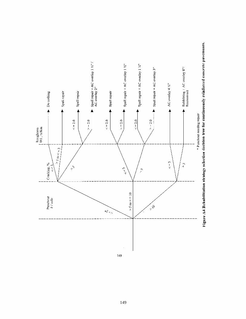
149