Embed Size (px)
Citation preview
REPORT CDOT-2021-08 FEBRUARY 2021
IN-SITU MONITORING OF INFILTRATION-INDUCED INSTABILITY OF I-70 EMBANKMENT WEST OF THE EISENHOWER-JOHNSON MEMORIAL TUNNELS, PHASE III
APPLIED RESEARCH &
INNOVATION BRANCH
Alexandra Wayllace, CSM Ning Lu, CSM Benjamin Mirus, USGS

IED RESEARCH & INNOVATION BRANCH Lu The contents of this report reflect the views of the author(s), who is(are)
responsible for the facts and accuracy of the data presented herein. The
contents do not necessarily reflect the official views of the Colorado
Department of Transportation or the Federal Highway Administration. This
report does not constitute a standard, specification, or regulation.

Technical Report Documentation Page 1. Report No. 2. Government Accession No. 3. Recipient's Catalog No.
4. Title and SubtitleIN-SITU MONITORING OF INFILTRATION-INDUCED INSTABILITY OF I-70 EMBANKMENT WEST OF THE EISENHOWER-JOHNSON MEMORIAL TUNNELS, PHASE III
5. Report DateFebruary 2021 6. Performing Organization Code
7. Author(s)Alexandra Wayllace, Ning Lu, Benjamin Mirus
8. Performing Organization Report No.
9. Performing Organization Name and Address 10. Work Unit No. (TRAIS)
11. Contract or Grant No.411013042
12. Sponsoring Agency Name and AddressColorado Department of Transportation - Research 4201 E. Arkansas Ave. Denver, CO 80222
13. Type of Report and Period CoveredFinal Draft
14. Sponsoring Agency Code
15. Supplementary Notes
16. AbstractA new methodology that uses recent advances in unsaturated soil mechanics and hydrology was developed and tested. The approach consists of using soil suction and moisture content field information in the prediction of the likelihood of landslide movement. The testing ground was an active landslide on I-70 west of the Eisenhower/Johnson Memorial Tunnels. A joint effort between Colorado School of Mines, CDOT, and USGS performed detailed site characterization, set up and calibrated a hydro-mechanical model of the site based on seven years of field data, and performed a stability analysis of the slope. Results indicate that consecutive years of high or low infiltration have a compounding effect so that the slope stability is influenced by the preceding years. Additionally, a new drainage system is proposed based on analysis of the current horizontal drains.
17. KeywordsInfiltration-induced landslides, unsaturated soils, CDOT
18. Distribution StatementThis document is available on CDOT’s website http://www.coloradodot.info/programs/research/pdfs
19. Security Classif. (of this report) Unclassified
20. Security Classif. (of this page)Unclassified
21. No. of Pages 22. Price
Form DOT F 1700.7 (8-72) Reproduction of completed page authorized
CDOT 2021-08
Colorado School of Mines1500 Illinois St. Golden, CO 80401
ii
In-situ Monitoring of Infiltration-induced Instability of I-70 Embankment West of the
Eisenhower-Johnson Memorial Tunnels, Phase III
Principal Investigator:
Dr. Alexandra Wayllace, Colorado School of Mines
Co-Principal Investigator:
Dr. Ning Lu, Colorado School of Mines
In collaboration with:
Benjamin Mirus, USGS Landslide Hazards Team
Submitted to:
Thien Tran, P.E.
e-mail: [email protected]
Research Engineer
CDOT-DTD Applied Research and Innovation Branch
2829 W. Howard Place
Denver, CO 80204
February 2021

iii
ACKNOWLEDGEMENTS The authors would like to thank the study panel members of the three phases of this project: Aziz
Khan, Grant Anderson, Russel Cox, Matt Greer, Tonya Hart, Hsing-Cheng Liu, Amanullah
Mommandi, William Scheuerman, David Thomas, Mark Vessely, and Trever Wang. We are also
very thankful to the various CDOT and USGS personnel that provided very valuable input
during the research progress meetings and site visits: Alfred Gross, David Novak, and Ty Ortiz.
We are grateful for the technical review of this report provided by Emily Bedinger (USGS) and
Thien Tran (CDOT). Most importantly, we would also like to acknowledge the hard work of the
graduate student that worked on this project: Eric Hinds. Any use of trade, firm, or product
names is for descriptive purposes only and does not imply endorsement by the U.S. Government.
iv
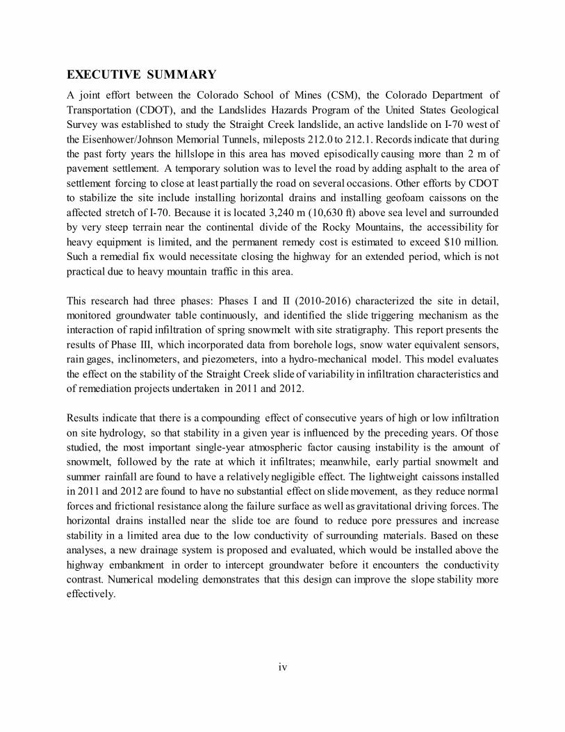
EXECUTIVE SUMMARY A joint effort between the Colorado School of Mines (CSM), the Colorado Department of Transportation (CDOT), and the Landslides Hazards Program of the United States Geological Survey was established to study the Straight Creek landslide, an active landslide on I-70 west of the Eisenhower/Johnson Memorial Tunnels, mileposts 212.0 to 212.1. Records indicate that during the past forty years the hillslope in this area has moved episodically causing more than 2 m of pavement settlement. A temporary solution was to level the road by adding asphalt to the area of settlement forcing to close at least partially the road on several occasions. Other efforts by CDOT to stabilize the site include installing horizontal drains and installing geofoam caissons on the affected stretch of I-70. Because it is located 3,240 m (10,630 ft) above sea level and surrounded by very steep terrain near the continental divide of the Rocky Mountains, the accessibility for heavy equipment is limited, and the permanent remedy cost is estimated to exceed $10 million. Such a remedial fix would necessitate closing the highway for an extended period, which is not practical due to heavy mountain traffic in this area.
This research had three phases: Phases I and II (2010-2016) characterized the site in detail, monitored groundwater table continuously, and identified the slide triggering mechanism as the interaction of rapid infiltration of spring snowmelt with site stratigraphy. This report presents the results of Phase III, which incorporated data from borehole logs, snow water equivalent sensors, rain gages, inclinometers, and piezometers, into a hydro-mechanical model. This model evaluates the effect on the stability of the Straight Creek slide of variability in infiltration characteristics and of remediation projects undertaken in 2011 and 2012.
Results indicate that there is a compounding effect of consecutive years of high or low infiltration on site hydrology, so that stability in a given year is influenced by the preceding years. Of those studied, the most important single-year atmospheric factor causing instability is the amount of snowmelt, followed by the rate at which it infiltrates; meanwhile, early partial snowmelt and summer rainfall are found to have a relatively negligible effect. The lightweight caissons installed in 2011 and 2012 are found to have no substantial effect on slide movement, as they reduce normal forces and frictional resistance along the failure surface as well as gravitational driving forces. The horizontal drains installed near the slide toe are found to reduce pore pressures and increase stability in a limited area due to the low conductivity of surrounding materials. Based on these analyses, a new drainage system is proposed and evaluated, which would be installed above the highway embankment in order to intercept groundwater before it encounters the conductivity contrast. Numerical modeling demonstrates that this design can improve the slope stability more effectively.
v
TABLE OF CONTENTS 1. INTRODUCTION AND BACKGROUND.....................................................................1
2. RESEARCH TASKS ......................................................................................................3
3. TASK I: FIELD MONITORING CONTINUATION AND IMPROVEMENT .............3
4. TASK II: HYDROLOGICAL AND SLOPE STABILITY ANALYSIS ......................13
5. TASK III: MITIGATION TECHNIQUES EVALUATION .........................................34
6. TASK IV: EVALUATION OF DRAIN SYSTEM NORTH OF I-70 ...........................48
7. SUMMARY AND CONCLUSIONS ............................................................................54
8. FURTHER ACTIONS ...................................................................................................56
9. REFERENCES ..............................................................................................................58
APPENDIX A: CSM BOREHOLE LOGS.................................................................... A-1
APPENDIX B: FIELD INSTRUMENTATION SET UP ...............................................B-1
APPENDIX C: LIST OF *.CSV DATA FILES .............................................................C-1
1
1. INTRODUCTION AND BACKGROUND
Landslides on highway embankments and nearby hillslopes are common geologic hazards to
transportation corridors in Colorado. Currently, the Colorado Department of Transportation
(CDOT) has identified 124 such landslides, many of which move annually and are reportedly
induced by infiltration of rainfall or snowmelt. When these slopes fail, they threaten public safety
and private property, block highway traffic, and damage transportation infrastructure. Instability
of these slopes in many cases results from infiltration of snowmelt and rainfall into variably
saturated hillslope soil and rock materials. As water infiltrates into the soil, the water content and
suction of the soil change and the water table position varies leading to a change in effective stress
throughout the slope. These changes then drive changes in the stability of the slope. Estimates of
the costs to reduce the risk to a moderate level often exceed tens of millions of dollars per slide,
creating a strong public interest in maximizing the efficacy and minimizing the cost of
interventions. Thus, it is important to understand the main mechanisms that affect the hillslope
stability and the effects of intervention projects. With this goal, a joint effort between CDOT, the
Colorado School of Mines (CSM), and the U.S. Geological Survey Landslides Hazard Program
(USGS-LHP) was initiated in 2010 to investigate the Straight Creek landslide, an active landslide
located in Summit County on I-70 west of the Eisenhower/Johnson Memorial Tunnels, mileposts
212.0 to 212.1.
The Straight Creek landslide, located on a steep south facing slope, is classified as “large” (width
> 500 ft and depth > 50 ft) by CDOT and has experienced episodic annual movement since 1973.
The relevant stretch of I-70 has an average daily traffic of over 20,000 vehicles and is important
to the trucking and tourism industries because alternative routes are steep, narrow, and not viable
for larger trucks. Large-scale remediation projects are not feasible because they would require
closing the highway for an impractical amount of time. The embankment was constructed in the
1960s; shortly after, several landslides occurred, and Robinson & Associates was hired to perform
a geotechnical investigation of the area (Robinson, 1971). In 1973, a bulge appeared near the
eastbound lanes of the highway; soon after, downslope movement occurred, causing measurable
road subsidence. The investigation identified excess pore water pressures as the cause of failure,
and a draining system was installed about 2 m below the surface; unfortunately, this system was
destroyed in 1979 during the widening of the embankment (Kumar & Associates, 1997). A
2
temporary measure to maintain a road leveled surface was asphalt capping; however, this measure
was not efficient because it had to be done several times per year, causing partial road closures. In
1996, CDOT commissioned Kumar & Associates to perform a more detailed investigation. Their
report indicates an ongoing slide failure, identifies the shear zone, and provides stratigraphic
information from six boreholes drilled on the west and eastbound shoulders of the highway, as
well as near the toe of the slide. In 2007 and 2008, CDOT installed inclinometers in the east and
westbound shoulders of the affected I-70 stretch; the sensors maxed out within a year, measuring
over 5 cm of lateral displacement. In 2011 and 2012, Shannon & Wilson, Inc. installed lightweight
caissons in the highway, and ten horizontal drains near the slide toe, to decrease normal stresses
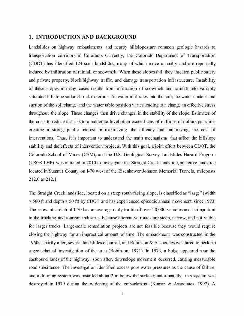
on the failure plane and pore water pressures in the hillslope. Figure 1a portrays the slide location
and extents.
The CSM-CDOT-USGS investigation was implemented in three phases. Phase I was an effort to
understand the environmental setting and triggering mechanism of the failure, which included
mapping of the failure zone, a subsurface investigation, and installation of sensors that have
continuously monitored groundwater behavior and ground movements in the slope since 2011.
Phase II aimed to fully understand the seasonal hydrology that leads to mechanical instability. All
available information on stratigraphy, construction at this location, and known water table levels,
was used to create an extended geological cross section of the entire watershed area and a
conceptual model of the annual hydrology, which was incorporated into a 2-dimensional numerical
model. The results of the hydrological model were then used in a preliminary slope stability
analysis to assess the local factor of safety in the slope under the different hydrological conditions
and confirm that movements in the slope are triggered by the large amount of infiltration into the
slope during the spring season (CDOT report 2017-12). This report presents the findings of Phase
III, which involves installing additional field instrumentation, gathering additional data on
atmospheric and groundwater conditions, and extending stability analyses to consider the
spatiotemporal evolution of instability using a local factor of safety concept incorporated into
hydro-mechanical modeling. The purpose of Phase III is to resolve uncertainty about where the
failure surface intersects the roadway, to characterize the effect on site hydrology and stability of
annual variability and multi-year patterns in infiltration characteristics, to assess the impact of the
3
remediation work conducted in 2011 and 2012, and to propose and evaluate a new, more targeted
remediation design.
The content of this report uses material published in the following documents:
i) Hinds, E. (2018). Effects of atmospheric variability and remediation techniques on the stability
of an interstate highway embankment. M.S. Thesis, Colorado School of Mines: Golden, CO,
167 pp. https://hdl.handle.net/11124/172344
ii) Hinds, E., Lu, N., Mirus, B., and Wayllace, A. (2019). “Effects of Infiltration Characteristics
on Spatial-Temporal Evolution of Stability of an Interstate Highway Embankment.” Journal
of Geotechnical and Geoenvironmental Engineering, 145(9): 05019008.
https://doi.org/10.1061/(ASCE)GT.1943-5606.0002127
iii) Wayllace, A., Thunder, B., Lu, N., Khan, A., and Godt, J. W. (2019). “Hydrological Behavior
of an Infiltration-Induced Landslide in Colorado, USA.” Geofluids, 2019: 1959303.
https://doi.org/10.1155/2019/1659303
iv) Hinds, E., Lu, N., Mirus, B. B., and Wayllace, A. (2021). “Effects of Infiltration Characteristics
on Spatial-Temporal Evolution of Stability of an Interstate Highway Embankment.”
Engineering Geology, 2021: Volume 291, 106240.
https://doi.org/10.1016/j.enggeo.2021.106240
2. RESEARCH TASKS
Five main tasks were identified during Phase III of this project:
Task I: Field monitoring continuation and improvement
Task II: Hydrological and slope stability analysis
Task III: Mitigation techniques evaluation
Task IV: Recommendations for site remediation
Task V: Draft report and final report
3. TASK I: FIELD MONITORING CONTINUATION AND IMPROVEMENT
3.1 Site description and instrumentation
The study site is located in Summit County on I-70 west of the Eisenhower/Johnson Memorial
Tunnels, mileposts 212.0 to 212.1 (Figure 1a). At an elevation of approximately 3,252 m (10,670

4
ft) above sea level and with a roughly 30° inclination, the slide mass is approximately 175 m wide
and 123 m long.
During Phase I and Phase II of this project, site characterization and instrumentation included
drilling four boreholes, laboratory testing of shear strength and hydrological properties of
relatively undisturbed samples, and installing 2 inclinometers and 4 vibrating wire piezometers. In
Phase III, the data obtained from that instrumentation was monitored and analyzed; furthermore,
four additional boreholes were drilled, and four vibrating wire piezometers were installed (Figure
1b). Logs from all boreholes conducted since 2010 as part of this investigation are included in
Appendix A.
A two-dimensional soil profile along a centerline transect through the slide is shown in Figure 2;
this information and the general characteristics of each material were derived from borehole logs
from past investigations (Lovering, 1935; Robinson & Associates, 1971; Kumar & Associates,
1997; Thunder, 2016), core sample testing (Thunder, 2016), and the 4 boreholes drilled during the
current study. The bedrock is primarily massive dark gneiss with occasional pegmatite and mica
intrusions, which is mostly competent and relatively impermeable compared with overlying
materials. The bedrock surface is generally parallel to the ground surface, although it is more
steeply inclined towards the west in the western half of the slide. Overlying the competent bedrock
is a layer of fractured and weathered material derived from the same dark gneiss, varying in
thickness from 1 m to close to 30 m. The degree of weathering increases further down the slope;
therefore, this layer was divided into two groups for the conceptual and numerical analysis. The
first group, called fractured gneiss, is found on the slope above the embankment; it presents clean
fracture surfaces with little weathering or infill and has high frictional strength and hydraulic
conductivity. The second group, called decomposed gneiss, is found underneath the embankment
and to the south of it. This material displays a higher degree of weathering, with lower strength
and hydraulic conductivity than the fractured gneiss material. Surficial soil on the slope consists
of colluvial deposits with angular, coarse sand to cobble-sized grains derived from the gneiss
bedrock. Alluvial soil on the valley floor is more uniform, consisting of rounded sand-sized grains.
Mechanical properties for the two materials are similar, but the hydraulic conductivity of the
colluvium is higher due to a lower in situ density caused by depositional processes. The tunnel-

5
cuttings material used for embankment fill is extremely heterogeneous, including large rock
fragments and boulders, construction rubble (such as decomposing timbers from shoring), and
more fine-grained material than the surrounding native soils. Hydraulic conductivity of this
material is very low due to this fines content. The embankment fill is approximately 14 m thick
under the westbound shoulder of I-70, approximately 29 m thick under the eastbound shoulder,
and extends approximately 61 m downslope (Hinds, 2018).
6
(a)
(b)
Figure 1. (a) Straight Creek slide location and extents; approximate slide area is shaded in red, approximate watershed area is outlined in blue and A-A’ transect shown in subsequent figures. (b) Piezometer locations with approximate slide extents shown in black (from Hinds, 2018).

7
Figure 2. Transect showing subsurface material distribution along the slide centerline shown in A-A’ transect in Figure 1 (from Hinds, et al., 2019).
3.2 Groundwater table variations
During the first and second phases of this project, it was clearly established that the hydrology of
the hillslope, particularly the dynamic changes in the groundwater table, was a key factor in the
stability of the slope (Wayllace et al., 2012, Wayllace et al., 2019).
Groundwater data in the first phase included the installation of three piezometers (P1, P2, and P3);
it was then evident that to better characterize hydrologic behavior, more information was needed
on the slope north of I-70, so a fourth piezometer (P4) was installed during Phase II. Four
additional piezometers were installed over the summer of 2017; these were distributed laterally
over the north slope. The depths below ground surface and installation date of all piezometers are
provided in Table 1; the piezometers’ locations are provided in Figure 1b. Piezometers P1 and P2
connected to a data logger near the toe of the slide, whereas piezometers P3-P8 connected to a data
logger located on the Westbound shoulder of I-70. Interruptions in the data occurred sometimes
over the winter season, as snow and deadfall often disrupt the cabled connections. The details on
the installation of the equipment are provided in Appendix B.
8
Table 1. List of Piezometers, installation depth and dates.
Number Name Date Installed
Depth [m]
P1 WB 10/24/2011 17.4 P2 Toe 10/14/2011 9.0 P3 EB 8/9/2012 33.5 P4 North 4/7/2016 15.2 P5 WB-East 8/4/2017 34.0 P6 WB-West 8/4/2017 36.1 P7 North-West 8/4/2017 18.5 P8 North-East 8/16/2017 17.1
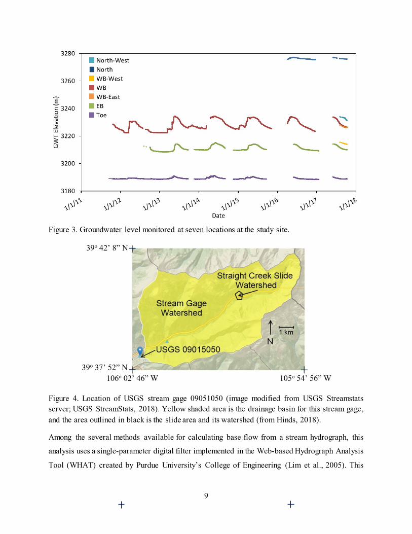
The data obtained with the piezometers is reported in Figure 3, where the ground water table
(GWT) elevations are calculated based on the measured pressure head, the location of the
instrument, and the installation depth. In general, the observations for piezometers P1-P3 are
consistent with previous years: Groundwater table near the westbound shoulder (P1) varies eight
to ten meters per year, while only ~30m across, near the eastbound shoulder, the variations of
groundwater table (P3) are half as much (4m – 5m). Near the toe of the slide, water table variations
throughout the year (P2) range between 1 m and 2 m. Measurements from the north area of I-70
are consistent with previous conceptual models (Wayllace et al., 2019); the water table varies from
1 m to 2 m throughout a year, confirming a material north of I-70 with larger hydraulic conductivity
than the material underneath the highway.
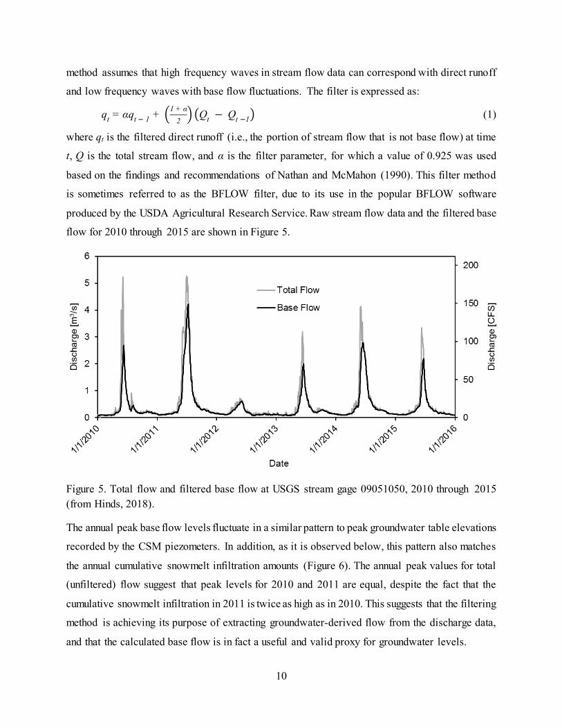
In addition to the piezometer data, this study also used data obtained from a stream gage
maintained by USGS; the stream gage, USGS 09051050, is located on Straight Creek
approximately 7.8 km west-southwest from the slide site (Figure 4). Even though there are
limitations on using this data, the base flow is generated by—and therefore a useful proxy for—
groundwater levels.
9
Figure 3. Groundwater level monitored at seven locations at the study site.
Figure 4. Location of USGS stream gage 09051050 (image modified from USGS Streamstats server; USGS StreamStats, 2018). Yellow shaded area is the drainage basin for this stream gage, and the area outlined in black is the slide area and its watershed (from Hinds, 2018).
Among the several methods available for calculating base flow from a stream hydrograph, this
analysis uses a single-parameter digital filter implemented in the Web-based Hydrograph Analysis
Tool (WHAT) created by Purdue University’s College of Engineering (Lim et al., 2005). This
10
method assumes that high frequency waves in stream flow data can correspond with direct runoff
and low frequency waves with base flow fluctuations. The filter is expressed as:
qt = αqt − 1 + �1 + α2� �Qt − Qt −1� (1)
where qt is the filtered direct runoff (i.e., the portion of stream flow that is not base flow) at time
t, Q is the total stream flow, and α is the filter parameter, for which a value of 0.925 was used
based on the findings and recommendations of Nathan and McMahon (1990). This filter method
is sometimes referred to as the BFLOW filter, due to its use in the popular BFLOW software
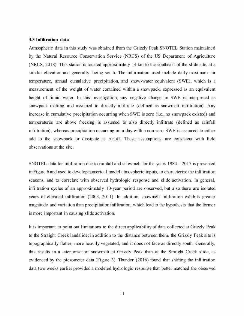
produced by the USDA Agricultural Research Service. Raw stream flow data and the filtered base
flow for 2010 through 2015 are shown in Figure 5.
Figure 5. Total flow and filtered base flow at USGS stream gage 09051050, 2010 through 2015 (from Hinds, 2018).
The annual peak base flow levels fluctuate in a similar pattern to peak groundwater table elevations
recorded by the CSM piezometers. In addition, as it is observed below, this pattern also matches
the annual cumulative snowmelt infiltration amounts (Figure 6). The annual peak values for total
(unfiltered) flow suggest that peak levels for 2010 and 2011 are equal, despite the fact that the
cumulative snowmelt infiltration in 2011 is twice as high as in 2010. This suggests that the filtering
method is achieving its purpose of extracting groundwater-derived flow from the discharge data,
and that the calculated base flow is in fact a useful and valid proxy for groundwater levels.
11
3.3 Infiltration data
Atmospheric data in this study was obtained from the Grizzly Peak SNOTEL Station maintained
by the Natural Resource Conservation Service (NRCS) of the US Department of Agriculture
(NRCS, 2018). This station is located approximately 14 km to the southeast of the slide site, at a
similar elevation and generally facing south. The information used include daily maximum air
temperature, annual cumulative precipitation, and snow-water equivalent (SWE), which is a
measurement of the weight of water contained within a snowpack, expressed as an equivalent
height of liquid water. In this investigation, any negative change in SWE is interpreted as
snowpack melting and assumed to directly infiltrate (defined as snowmelt infiltration). Any
increase in cumulative precipitation occurring when SWE is zero (i.e., no snowpack existed) and
temperatures are above freezing is assumed to also directly infiltrate (defined as rainfall
infiltration), whereas precipitation occurring on a day with a non-zero SWE is assumed to either
add to the snowpack or dissipate as runoff. These assumptions are consistent with field
observations at the site.
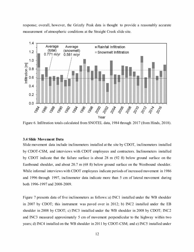
SNOTEL data for infiltration due to rainfall and snowmelt for the years 1984 – 2017 is presented
in Figure 6 and used to develop numerical model atmospheric inputs, to characterize the infiltration
seasons, and to correlate with observed hydrologic response and slide activation. In general,
infiltration cycles of an approximately 10-year period are observed, but also there are isolated
years of elevated infiltration (2003, 2011). In addition, snowmelt infiltration exhibits greater
magnitude and variation than precipitation infiltration, which lead to the hypothesis that the former
is more important in causing slide activation.
It is important to point out limitations to the direct applicability of data collected at Grizzly Peak
to the Straight Creek landslide; in addition to the distance between them, the Grizzly Peak site is
topographically flatter, more heavily vegetated, and it does not face as directly south. Generally,
this results in a later onset of snowmelt at Grizzly Peak than at the Straight Creek slide, as
evidenced by the piezometer data (Figure 3). Thunder (2016) found that shifting the infiltration
data two weeks earlier provided a modeled hydrologic response that better matched the observed
12
response; overall, however, the Grizzly Peak data is thought to provide a reasonably accurate
measurement of atmospheric conditions at the Straight Creek slide site.
Figure 6. Infiltration totals calculated from SNOTEL data, 1984 through 2017 (from Hinds, 2018).
3.4 Slide Movement Data Slide movement data include inclinometers installed at the site by CDOT, inclinometers installed
by CDOT-CSM, and interviews with CDOT employees and contractors. Inclinometers installed
by CDOT indicate that the failure surface is about 28 m (92 ft) below ground surface on the
Eastbound shoulder, and about 20.7 m (68 ft) below ground surface on the Westbound shoulder.
While informal interviews with CDOT employees indicate periods of increased movement in 1986
and 1996 through 1997, inclinometer data indicate more than 5 cm of lateral movement during
both 1996-1997 and 2008-2009.
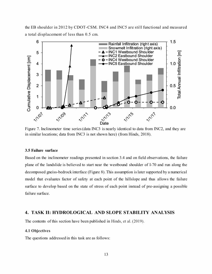
Figure 7 presents data of five inclinometers as follows: a) INC1 installed under the WB shoulder
in 2007 by CDOT; this instrument was paved over in 2012; b) INC2 installed under the EB
shoulder in 2008 by CDOT; c) INC3 installed under the WB shoulder in 2008 by CDOT; INC2
and INC3 measured approximately 5 cm of movement perpendicular to the highway within two
years; d) INC4 installed on the WB shoulder in 2011 by CDOT-CSM; and e) INC5 installed under
13
the EB shoulder in 2012 by CDOT-CSM. INC4 and INC5 are still functional and measured
a total displacement of less than 0.5 cm.
Figure 7. Inclinometer time series (data INC3 is nearly identical to data from INC2, and they are in similar locations; data from INC3 is not shown here) (from Hinds, 2018).
3.5 Failure surface
Based on the inclinometer readings presented in section 3.4 and on field observations, the failure
plane of the landslide is believed to start near the westbound shoulder of I-70 and run along the
decomposed gneiss-bedrock interface (Figure 8). This assumption is later supported by a numerical
model that evaluates factor of safety at each point of the hillslope and thus allows the failure
surface to develop based on the state of stress of each point instead of pre-assigning a possible
failure surface.
4. TASK II: HYDROLOGICAL AND SLOPE STABILITY ANALYSIS
The contents of this section have been published in Hinds, et al. (2019). 4.1 Objectives
The questions addressed in this task are as follows:
14
A) How sensitive is embankment stability to annual variability in infiltration characteristics,
including the total annual cumulative infiltration from snowmelt and rainfall, the rate at
which that infiltration occurs, and variability in its timing?
B) Can infiltration conditions in previous years affect site hydrology and embankment stability
during a given year?
C) Can infiltration characteristics be used to predict instability?
Because the landslide is a recurring failure that continually crosses between stable and unstable
states, failing in essentially the same mode every year, albeit to varying degrees; a sensitivity
analysis of the embankment’s stability can help answer the questions above. This investigation
develops an approach to quantify the controls on the activation length of recurring infiltration-
triggered landslides and thereby identify physics-based thresholds for reactivation. The resulting
insights contribute to understanding the specific trigger mechanisms and levels of risk for other
similar sites.
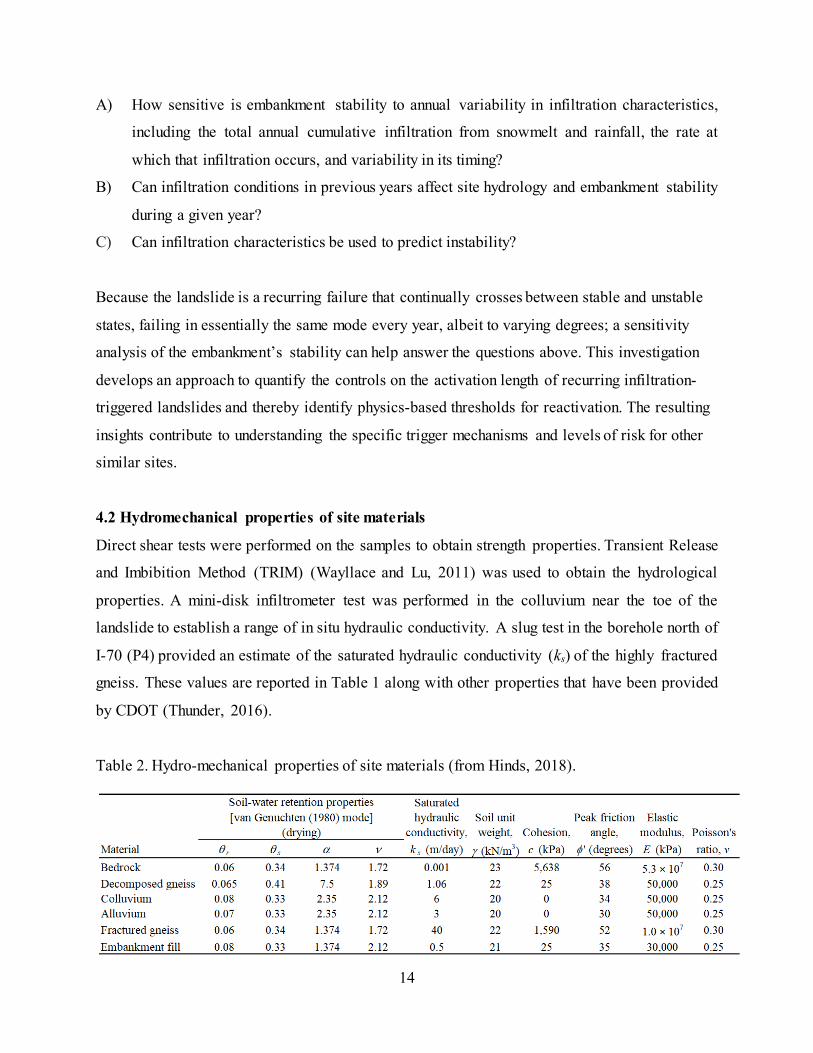
4.2 Hydromechanical properties of site materials
Direct shear tests were performed on the samples to obtain strength properties. Transient Release
and Imbibition Method (TRIM) (Wayllace and Lu, 2011) was used to obtain the hydrological
properties. A mini-disk infiltrometer test was performed in the colluvium near the toe of the
landslide to establish a range of in situ hydraulic conductivity. A slug test in the borehole north of
I-70 (P4) provided an estimate of the saturated hydraulic conductivity (ks) of the highly fractured
gneiss. These values are reported in Table 1 along with other properties that have been provided
by CDOT (Thunder, 2016).
Table 2. Hydro-mechanical properties of site materials (from Hinds, 2018).
15
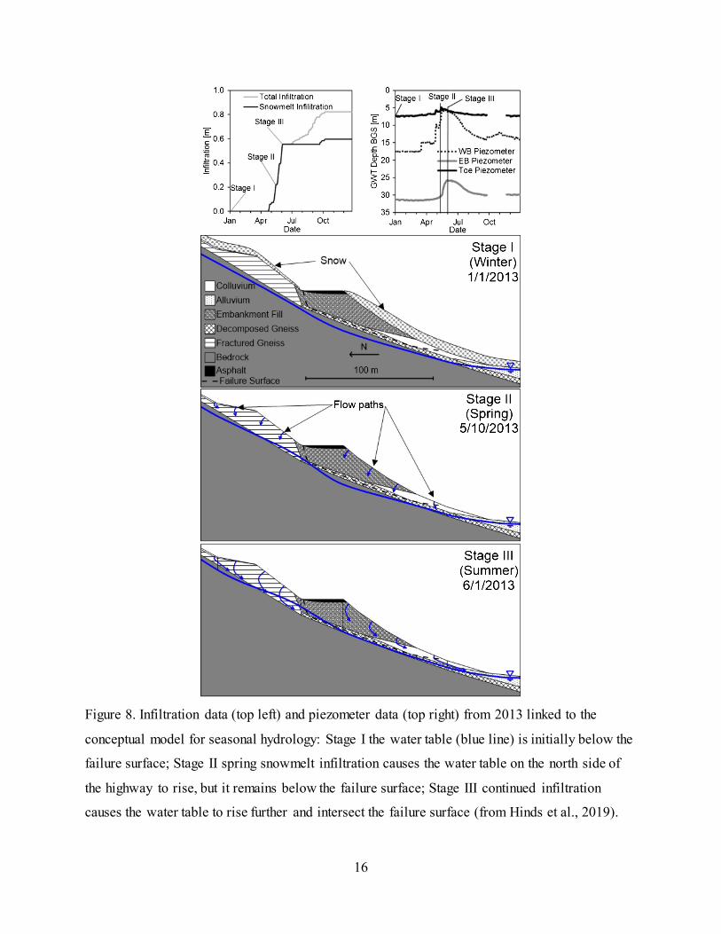
4.3 Conceptual model of seasonal hydrology
The following conceptual model was presented in Phase II and consists of three seasonal stages
(Lu et al., 2013). Stage I coincides with winter; in this stage the groundwater table is at its lowest
level, resting along the surface of the competent bedrock. During this stage snowpack accumulates
with essentially no melting or other infiltration occurring. Stage II corresponds to the spring;
during this stage rapid melting of the snowpack occurs, and the meltwater begins to infiltrate into
the hillslope. In most years, an initial fast increase in groundwater level is observed, probably due
to snow plowed onto the WB shoulder melting as the temperatures warm up. Subsurface flow is
initially perpendicular to the slope during this period because moisture gradients control flow
direction more than gravity (simulated pathlines near the slope surface in Figure 8); as the slope
becomes wetter, vertical flow predominates (simulated pathlines in the middle of the slope in
Figure 8). Stage III corresponds roughly to summer and fall, when the hillslope has higher
saturation and there is slower surface infiltration rate due to rainfall.
The hydrological observations at this site are unusual in that water table positions beneath the
westbound shoulder of the highway (upslope) varied twice as much as water table positions
beneath the eastbound shoulder (downslope), only 30m distant horizontally. This may be because
the hydraulic conductivity contrast between the fractured gneiss and competent bedrock layers
promotes lateral downslope flow along the bedrock interface north of I-70; this flow then
encounters the contrast in hydraulic conductivity between the fractured gneiss and embankment
material causing a rapid and pronounced elevation in groundwater levels underneath the
westbound lanes of the highway.
As the groundwater rise increases pore water pressures along the failure surface, effective stress
decreases or suction stress increases, resulting in shear strength reduction and slide activation.
During the fall, precipitation slows, and the hillslope drains out and approaches the winter-steady
state.
16
Figure 8. Infiltration data (top left) and piezometer data (top right) from 2013 linked to the
conceptual model for seasonal hydrology: Stage I the water table (blue line) is initially below the
failure surface; Stage II spring snowmelt infiltration causes the water table on the north side of
the highway to rise, but it remains below the failure surface; Stage III continued infiltration
causes the water table to rise further and intersect the failure surface (from Hinds et al., 2019).

17
4.4 Framework for numerical analysis
The hydro-mechanical framework used in this study was reported in Phase II. This rigorous, yet
simple approach accounts for the major physical processes in the slope: stress, deformation, and
variably saturated flow. In this framework, effective stress distributions used for the stability
analysis are calculated throughout the slope by taking into account the slope’s geomorphology, its
hydrology, and the stress, strain, and deformation. The transient hydrological and mechanical
behavior of the slope is analyzed by one-way coupling Richards’ equation (2) with classical linear-
elasticity equations.
𝜕𝜕𝜕𝜕𝜕𝜕�𝑘𝑘𝜕𝜕(ℎ𝑚𝑚) 𝜕𝜕ℎ𝑚𝑚
𝜕𝜕𝜕𝜕�+ 𝜕𝜕
𝜕𝜕𝜕𝜕�𝑘𝑘𝜕𝜕(ℎ𝑚𝑚) 𝜕𝜕ℎ𝑚𝑚
𝜕𝜕𝜕𝜕� + 𝜕𝜕
𝜕𝜕𝜕𝜕�𝑘𝑘𝜕𝜕(ℎ𝑚𝑚) �𝜕𝜕ℎ𝑚𝑚
𝜕𝜕𝜕𝜕+ 1�� = 𝐶𝐶(ℎ𝑚𝑚) 𝜕𝜕ℎ𝑚𝑚
𝜕𝜕𝜕𝜕 (2)
where hm is head, k(hm) is the hydraulic conductivity function (HCF), t is time, and C(hm) is the
specific moisture capacity function, or the slope of the SWRC.
The effective stress σ′for variably saturated porous materials is defined as (Lu and Likos, 2004):
( )Iσσ sau σ+−=' (3)
where σ is the total stress, ua is the pore air pressure, I is the second-order identity tensor, and σ s
is the suction stress that is a characteristic function of saturation or matric suction and is expressed
in a closed form for all soils (Lu and Likos, 2004, 2006):
0)( ≤−−−= wawas uuuuσ (4a)
( ) 0≥−−−= waewas uuSuuσ (4b)
where (ua – uw) is the matric suction, and Se is the equivalent degree of saturation. Using van
Genuchten’s model (1980) to describe the soil water retention curve, suction stress (equation (4b))
can be expressed as a sole function of matric suction (Lu and Likos, 2004; Lu et al., 2010):
( )
( )[ ]( ) ( ) nnnwa
was
uuuu
/11 −−+
−−=
ασ (4c)
where α and n are empirical fitting parameters in van Genuchten’s soil water retention model.
Once the total stress, matric suction, and suction stress distributions throughout the slope are
known, effective stress is calculated, and the stability of the slope can be calculated by taking into
account the shear strength properties of the soil combined with the effective stress distribution. Local factor of safety and Activated length
18
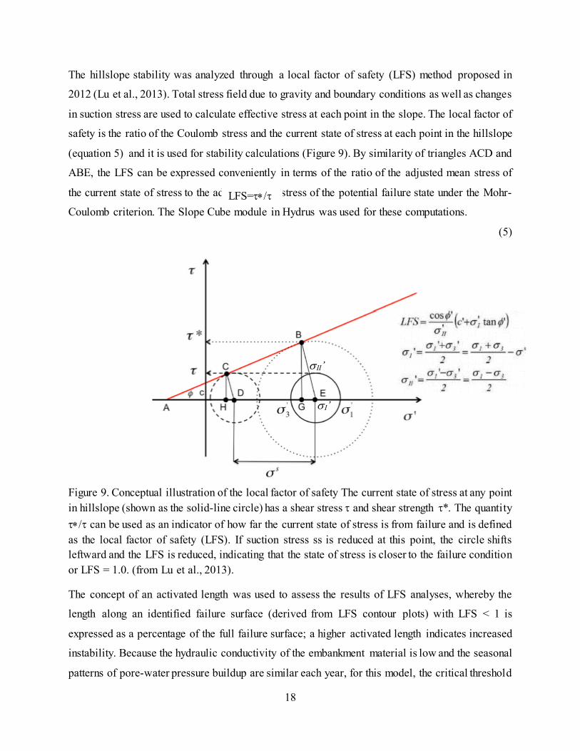
The hillslope stability was analyzed through a local factor of safety (LFS) method proposed in
2012 (Lu et al., 2013). Total stress field due to gravity and boundary conditions as well as changes
in suction stress are used to calculate effective stress at each point in the slope. The local factor of
safety is the ratio of the Coulomb stress and the current state of stress at each point in the hillslope
(equation 5) and it is used for stability calculations (Figure 9). By similarity of triangles ACD and
ABE, the LFS can be expressed conveniently in terms of the ratio of the adjusted mean stress of
the current state of stress to the adjusted mean stress of the potential failure state under the Mohr-
Coulomb criterion. The Slope Cube module in Hydrus was used for these computations.
(5)
Figure 9. Conceptual illustration of the local factor of safety The current state of stress at any point in hillslope (shown as the solid-line circle) has a shear stress τ and shear strength τ*. The quantity τ∗/τ can be used as an indicator of how far the current state of stress is from failure and is defined as the local factor of safety (LFS). If suction stress ss is reduced at this point, the circle shifts leftward and the LFS is reduced, indicating that the state of stress is closer to the failure condition or LFS = 1.0. (from Lu et al., 2013).
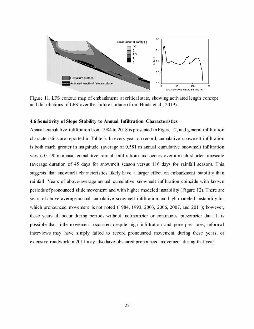
The concept of an activated length was used to assess the results of LFS analyses, whereby the
length along an identified failure surface (derived from LFS contour plots) with LFS < 1 is
expressed as a percentage of the full failure surface; a higher activated length indicates increased
instability. Because the hydraulic conductivity of the embankment material is low and the seasonal
patterns of pore-water pressure buildup are similar each year, for this model, the critical threshold
LFS=τ∗/τ
σI’
σII’
19
of activated length is identified by integrating the distribution of LFS over the identified failure
surface and finding the activated length at which this integration is equal to zero. Strength
parameters were adjusted so that this critical threshold (identified as 62.5% of the total failure
length along the failure surface) is just reached at two points, with the lowest simulated instability
corresponding to periods of known pronounced movement (the summers of 1986 and 2009).
4.5 Numerical model
The numerical model was conducted using HYDRUS 2D version 2.0 (Šimůnek et al., 2011), a
finite-element software that models groundwater hydrology by solving Richards’ equation
(Richards 1931). Hydrological soil properties are described using van Genuchten (1980) Soil
Water Retention Curve (SWRC) model and Mualem (1976) Hydraulic Conductivity Function
(HCF) models. The Slope Cube module of HYDRUS 2D (Lu et al., 2016) is used for all stress
field computation and stability analyses.
Model geometry was based on the transect in Figure 2, with the north boundary extended 740 m
up to the watershed boundary (Figure 1); this large extent of northern slope is needed to generate
the high lateral subsurface flux caused by infiltration over the entire slope up to the drainage divide.
The south boundary is also extended 100 m to reduce boundary effects in stress calculations. The
mechanical boundary conditions at both the north and south boundaries are no horizontal
displacement but free vertical displacement. The mechanical boundary conditions at the bottom
are no vertical displacement but free horizontal displacement. Based on site geologic and
hydrologic conditions, the hydrologic boundary conditions are set to no flux at (1) the bottom and
north boundaries due to the relative low hydraulic conductivity of the bedrock and intact rock, and
(2) the highway surface due to the relative impermeable layer of asphalts. A specified flux
boundary condition is used at the slope surface to allow applied infiltration for both rainfall and
snowmelt precipitation. A constant head is applied at the south boundary to reflect the modulating
effect of Straight Creek, which approximately coincides with that boundary. Although the water
level of Straight Creek may vary, the annual fluctuation is less than a few feet or a meter. The
effect of such change has a minimum effect on the groundwater table variation within the slope,
as indicated in the recorded data nearby at the toe of the slope shown in Figure 3. Material
properties reported in Table 2 were used.
20
Initial conditions were obtained by applying an average year of infiltration data created by
distributing the average accumulated infiltration for both spring snowmelt and summer rainfall
seasons over the average duration of these seasons. This gives rates of 0.0116 m/day during the
snowmelt season, which runs from April 1 to May 21, and 0.00152 m/day during the rainfall
season, which runs from May 22 to September 22. No infiltration is applied on the slope during
all other periods of the average year. This infiltration cycle was then applied for 60 years, which
is found to be sufficient for a steady cyclical state to be reached; this steady cyclical state was
defined as one in which, under steady annually cyclical infiltration, peak and minimum pressure
heads at the observation nodes do not change between years. This is therefore considered
appropriate as a representative initial hydrologic conditions for investigating sensitivity to annual
variability in infiltration. All model runs using these initial conditions begin on January 1.
The model was calibrated using the multiyear water table variation and the 2-week shift of
infiltration boundary condition. Infiltration data for the years over which piezometer data are
available; soil hydrologic properties and spatial distribution are then calibrated within ranges
constrained by the literature, previous laboratory testing programs, and interpretation of borehole
logs to match observed piezometer data as closely as possible. The hydrological simulation results
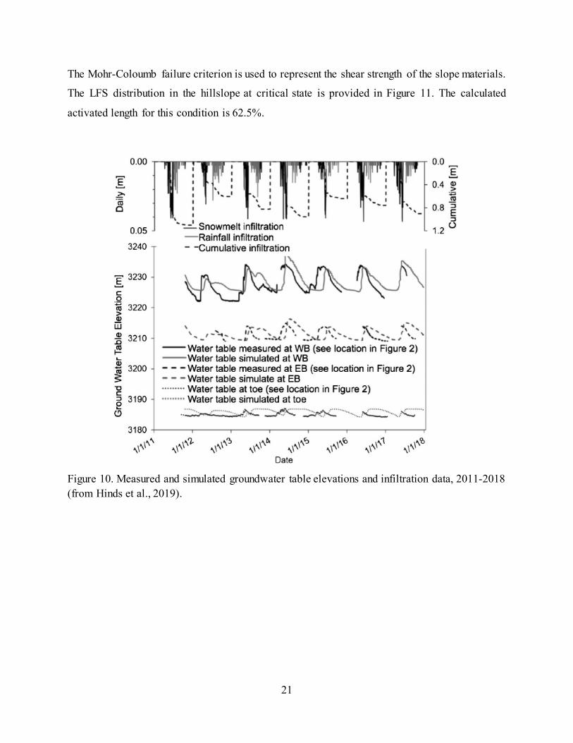
are shown in Figure 10 indicating that the use of the SNOTEL infiltration with the two week shift
is reasonable; the simulation and field measurements are closer to each other for the WB
piezometer than for the piezometers at the EB and near the toe of the slide. Annual peak pressure
heads, which are considered the most critical hydrologic result because they directly cause peak
instability, generally match piezometer data very well, as do annual minimum pressure heads; the
timing of pressure head change does not. Some discrepancy may be explained by differences
between the Straight Creek slide site and the SNOTEL station site, which is 14 km away in a
different (although similar) watershed, and in a location that is topographically flatter, more
heavily forested, and more distant from roadways than the Straight Creek slide. These differences
may be sufficient to cause the persistent disparity in timing and occasional disparity in magnitude
of groundwater level peaks.
21
The Mohr-Coloumb failure criterion is used to represent the shear strength of the slope materials.
The LFS distribution in the hillslope at critical state is provided in Figure 11. The calculated
activated length for this condition is 62.5%.
Figure 10. Measured and simulated groundwater table elevations and infiltration data, 2011-2018 (from Hinds et al., 2019).
22
Figure 11. LFS contour map of embankment at critical state, showing activated length concept and distributions of LFS over the failure surface (from Hinds et al., 2019).
4.6 Sensitivity of Slope Stability to Annual Infiltration Characteristics
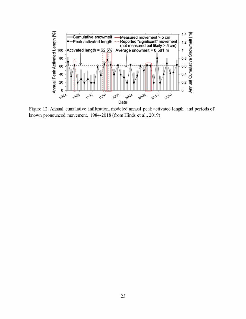
Annual cumulative infiltration from 1984 to 2018 is presented in Figure 12, and general infiltration
characteristics are reported in Table 3. In every year on record, cumulative snowmelt infiltration
is both much greater in magnitude (average of 0.581 m annual cumulative snowmelt infiltration
versus 0.190 m annual cumulative rainfall infiltration) and occurs over a much shorter timescale
(average duration of 45 days for snowmelt season versus 116 days for rainfall season). This
suggests that snowmelt characteristics likely have a larger effect on embankment stability than
rainfall. Years of above-average annual cumulative snowmelt infiltration coincide with known
periods of pronounced slide movement and with higher modeled instability (Figure 12). There are
years of above-average annual cumulative snowmelt infiltration and high-modeled instability for
which pronounced movement is not noted (1984, 1993, 2003, 2006, 2007, and 2011); however,
these years all occur during periods without inclinometer or continuous piezometer data. It is
possible that little movement occurred despite high infiltration and pore pressures; informal
interviews may have simply failed to record pronounced movement during these years, or
extensive roadwork in 2011 may also have obscured pronounced movement during that year.
23
Figure 12. Annual cumulative infiltration, modeled annual peak activated length, and periods of known pronounced movement, 1984-2018 (from Hinds et al., 2019).
24
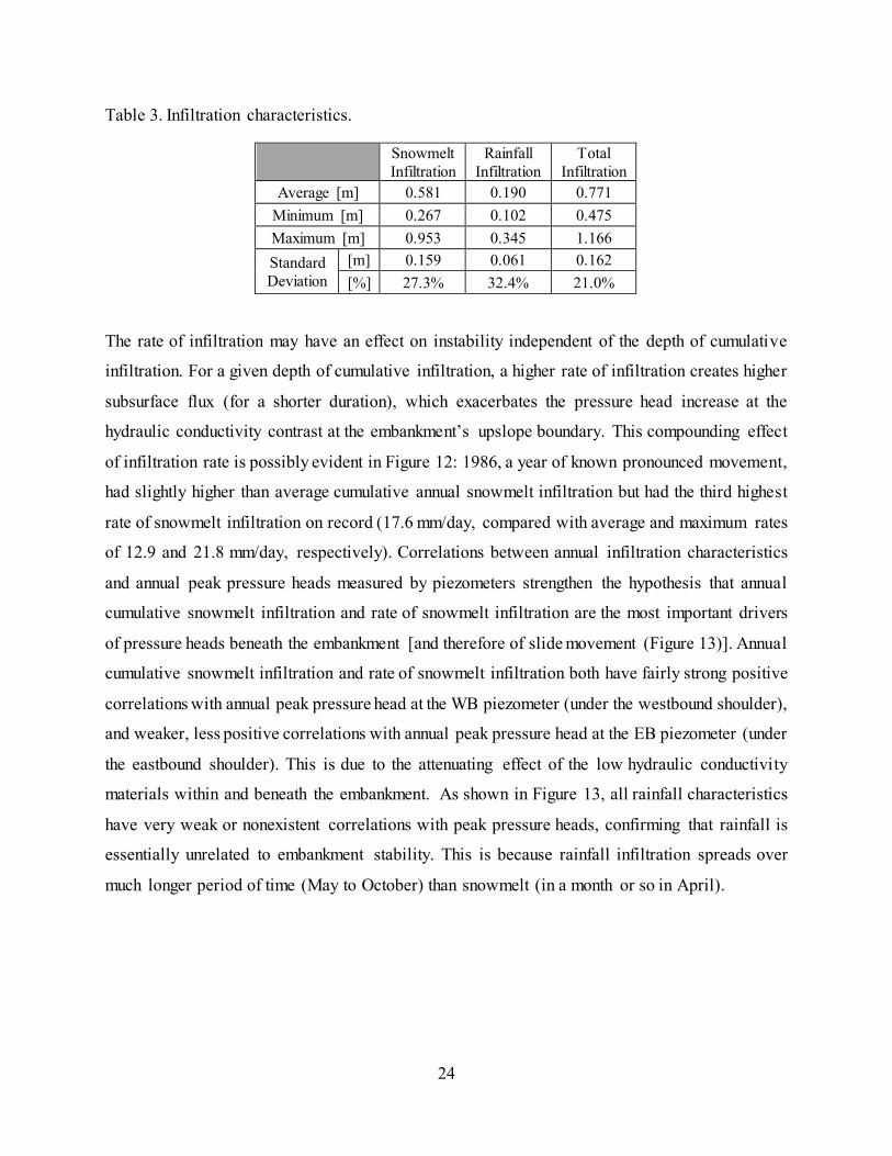
Table 3. Infiltration characteristics.
Snowmelt Infiltration
Rainfall Infiltration
Total Infiltration
Average [m] 0.581 0.190 0.771 Minimum [m] 0.267 0.102 0.475 Maximum [m] 0.953 0.345 1.166 Standard Deviation
[m] 0.159 0.061 0.162 [%] 27.3% 32.4% 21.0%
The rate of infiltration may have an effect on instability independent of the depth of cumulative
infiltration. For a given depth of cumulative infiltration, a higher rate of infiltration creates higher
subsurface flux (for a shorter duration), which exacerbates the pressure head increase at the
hydraulic conductivity contrast at the embankment’s upslope boundary. This compounding effect
of infiltration rate is possibly evident in Figure 12: 1986, a year of known pronounced movement,
had slightly higher than average cumulative annual snowmelt infiltration but had the third highest
rate of snowmelt infiltration on record (17.6 mm/day, compared with average and maximum rates
of 12.9 and 21.8 mm/day, respectively). Correlations between annual infiltration characteristics
and annual peak pressure heads measured by piezometers strengthen the hypothesis that annual
cumulative snowmelt infiltration and rate of snowmelt infiltration are the most important drivers
of pressure heads beneath the embankment [and therefore of slide movement (Figure 13)]. Annual
cumulative snowmelt infiltration and rate of snowmelt infiltration both have fairly strong positive
correlations with annual peak pressure head at the WB piezometer (under the westbound shoulder),
and weaker, less positive correlations with annual peak pressure head at the EB piezometer (under
the eastbound shoulder). This is due to the attenuating effect of the low hydraulic conductivity
materials within and beneath the embankment. As shown in Figure 13, all rainfall characteristics
have very weak or nonexistent correlations with peak pressure heads, confirming that rainfall is
essentially unrelated to embankment stability. This is because rainfall infiltration spreads over
much longer period of time (May to October) than snowmelt (in a month or so in April).
25
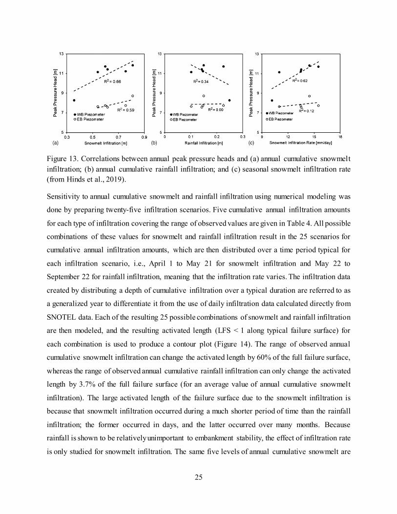
Figure 13. Correlations between annual peak pressure heads and (a) annual cumulative snowmelt infiltration; (b) annual cumulative rainfall infiltration; and (c) seasonal snowmelt infiltration rate (from Hinds et al., 2019).
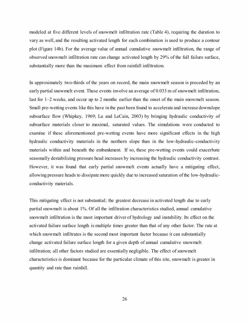
Sensitivity to annual cumulative snowmelt and rainfall infiltration using numerical modeling was
done by preparing twenty-five infiltration scenarios. Five cumulative annual infiltration amounts
for each type of infiltration covering the range of observed values are given in Table 4. All possible
combinations of these values for snowmelt and rainfall infiltration result in the 25 scenarios for
cumulative annual infiltration amounts, which are then distributed over a time period typical for
each infiltration scenario, i.e., April 1 to May 21 for snowmelt infiltration and May 22 to
September 22 for rainfall infiltration, meaning that the infiltration rate varies. The infiltration data
created by distributing a depth of cumulative infiltration over a typical duration are referred to as
a generalized year to differentiate it from the use of daily infiltration data calculated directly from
SNOTEL data. Each of the resulting 25 possible combinations of snowmelt and rainfall infiltration
are then modeled, and the resulting activated length (LFS < 1 along typical failure surface) for
each combination is used to produce a contour plot (Figure 14). The range of observed annual
cumulative snowmelt infiltration can change the activated length by 60% of the full failure surface,
whereas the range of observed annual cumulative rainfall infiltration can only change the activated
length by 3.7% of the full failure surface (for an average value of annual cumulative snowmelt
infiltration). The large activated length of the failure surface due to the snowmelt infiltration is
because that snowmelt infiltration occurred during a much shorter period of time than the rainfall
infiltration; the former occurred in days, and the latter occurred over many months. Because
rainfall is shown to be relatively unimportant to embankment stability, the effect of infiltration rate
is only studied for snowmelt infiltration. The same five levels of annual cumulative snowmelt are
26
modeled at five different levels of snowmelt infiltration rate (Table 4), requiring the duration to
vary as well, and the resulting activated length for each combination is used to produce a contour
plot (Figure 14b). For the average value of annual cumulative snowmelt infiltration, the range of
observed snowmelt infiltration rate can change activated length by 29% of the full failure surface,
substantially more than the maximum effect from rainfall infiltration.
In approximately two-thirds of the years on record, the main snowmelt season is preceded by an
early partial snowmelt event. These events involve an average of 0.033 m of snowmelt infiltration,
last for 1–2 weeks, and occur up to 2 months earlier than the onset of the main snowmelt season.
Small pre-wetting events like this have in the past been found to accelerate and increase downslope
subsurface flow (Whipkey, 1969; Lu and LeCain, 2003) by bringing hydraulic conductivity of
subsurface materials closer to maximal, saturated values. The simulations were conducted to
examine if these aforementioned pre-wetting events have more significant effects in the high
hydraulic conductivity materials in the northern slope than in the low-hydraulic-conductivity
materials within and beneath the embankment. If so, these pre-wetting events could exacerbate
seasonally destabilizing pressure head increases by increasing the hydraulic conductivity contrast.
However, it was found that early partial snowmelt events actually have a mitigating effect,
allowing pressure heads to dissipate more quickly due to increased saturation of the low-hydraulic-
conductivity materials.
This mitigating effect is not substantial; the greatest decrease in activated length due to early
partial snowmelt is about 1%. Of all the infiltration characteristics studied, annual cumulative
snowmelt infiltration is the most important driver of hydrology and instability. Its effect on the
activated failure surface length is multiple times greater than that of any other factor. The rate at
which snowmelt infiltrates is the second most important factor because it can substantially
change activated failure surface length for a given depth of annual cumulative snowmelt
infiltration; all other factors studied are essentially negligible. The effect of snowmelt
characteristics is dominant because for the particular climate of this site, snowmelt is greater in
quantity and rate than rainfall.
27
Table 4. Cumulative infiltration levels used in modeling synthesis (from Hinds et al., 2019).
Level 1 Level 2 Level 3 Level 4 Level 5 Infiltration characteristic (minimum) (average) (maximum) Annual cumulative rainfall (m) 0.102 0.146 0.190 0.268 0.345 Annual cumulative snowmelt (m) 0.267 0.424 0.581 0.767 0.953 Snowmelt infiltration rate (mm/day) 7.7 10.3 12.9 17.4 21.8
Figure 14. Contour plots of activated length modeled for various combinations of annual cumulative snowmelt infiltration and (a) rainfall infiltration; or (b) snowmelt infiltration rate (from Hinds et al., 2019).
4.7 Sensitivity of Slope Stability to Infiltration in Preceding Year
The effect of antecedent soil-moisture conditions on slope stability during infiltration has been
firmly established; long-term (seasonal to annual scale) conditions have also been identified as
particularly important (Campbell, 1975). Periods of known pronounced movement of the Straight
Creek slide tend to coincide not only with years of above-average annual cumulative snowmelt
infiltration, but also with periods of such years occurring consecutively (Figure 12). This suggests
that pre-snowmelt groundwater levels may be affected by infiltration in the previous year; a year
of above-average annual cumulative snowmelt infiltration may produce increased soil moisture
that does not drain out to the same state as after a year of average or below-average annual
cumulative snowmelt infiltration. This increase in antecedent soil-moisture conditions or
groundwater level, referred to as a carryover effect in soil moisture, may amplify the seasonal
28
increase in pressure heads following snowmelt infiltration, as reported in some other studies (e.g.,
Wieczorek and Glade, 2005).
The period for which piezometer data are available is too short to conduct a rigorous analysis of
this possible carryover effect. To expand the number of years available for analysis, a different
measure of or proxy for groundwater levels is necessary; data from USGS Stream Gauge 09051050
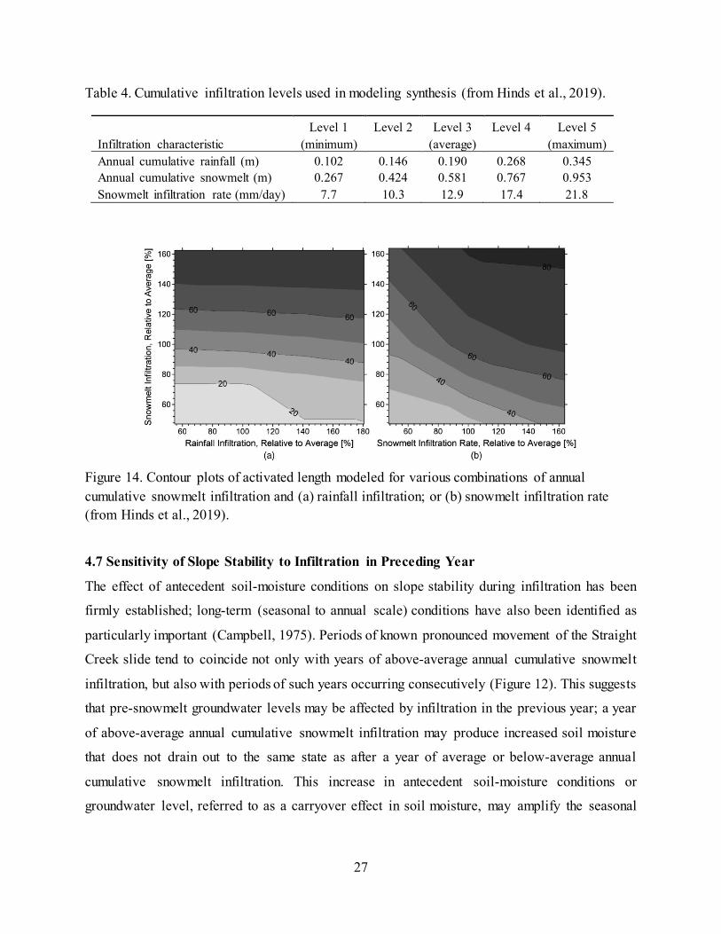
(USGS, 2018) was used for this purpose, as explained in Section 3.2 of this report. The average
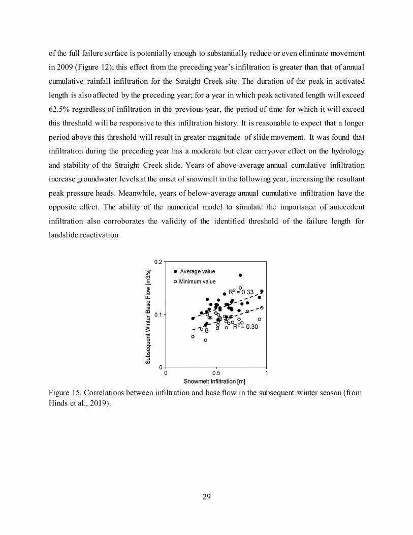
subsequent winter base flow and minimum subsequent winter base flow can then be correlated to
annual cumulative snowmelt infiltration; winter is defined as December 1 through March 31 for
this analysis. There is in fact a positive correlation between the snowmelt infiltration in a given
year and the base flow during the following winter (Figure 15). This correlation cannot completely
explain variation in wintertime base flow, but it could explain much of the variation. Some
discrepancy may be explained by the distance of both the stream gauge and SNOTEL site from
the slide, and by the drainage area of the stream gauge, which is much larger (47.7 versus 0.3 km2)
and more varied than the slide site watershed.
If the assumption that changes in base flow correspond to changes in groundwater level is valid,
then the proposed carryover effect seems likely to exist to some degree. The effect of infiltration
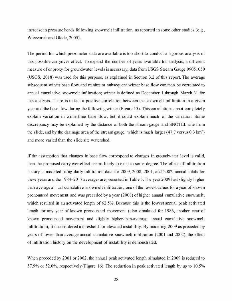
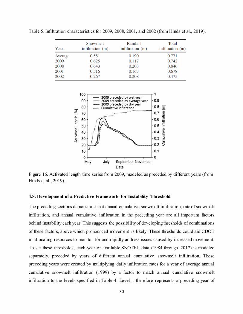
history is modeled using daily infiltration data for 2009, 2008, 2001, and 2002; annual totals for
these years and the 1984–2017 averages are presented in Table 5. The year 2009 had slightly higher
than average annual cumulative snowmelt infiltration, one of the lowest values for a year of known
pronounced movement and was preceded by a year (2008) of higher annual cumulative snowmelt,
which resulted in an activated length of 62.5%. Because this is the lowest annual peak activated
length for any year of known pronounced movement (also simulated for 1986, another year of
known pronounced movement and slightly higher-than-average annual cumulative snowmelt
infiltration), it is considered a threshold for elevated instability. By modeling 2009 as preceded by
years of lower-than-average annual cumulative snowmelt infiltration (2001 and 2002), the effect
of infiltration history on the development of instability is demonstrated.
When preceded by 2001 or 2002, the annual peak activated length simulated in 2009 is reduced to
57.9% or 52.0%, respectively (Figure 16). The reduction in peak activated length by up to 10.5%
29
of the full failure surface is potentially enough to substantially reduce or even eliminate movement
in 2009 (Figure 12); this effect from the preceding year’s infiltration is greater than that of annual
cumulative rainfall infiltration for the Straight Creek site. The duration of the peak in activated
length is also affected by the preceding year; for a year in which peak activated length will exceed
62.5% regardless of infiltration in the previous year, the period of time for which it will exceed
this threshold will be responsive to this infiltration history. It is reasonable to expect that a longer
period above this threshold will result in greater magnitude of slide movement. It was found that
infiltration during the preceding year has a moderate but clear carryover effect on the hydrology
and stability of the Straight Creek slide. Years of above-average annual cumulative infiltration
increase groundwater levels at the onset of snowmelt in the following year, increasing the resultant
peak pressure heads. Meanwhile, years of below-average annual cumulative infiltration have the
opposite effect. The ability of the numerical model to simulate the importance of antecedent
infiltration also corroborates the validity of the identified threshold of the failure length for
landslide reactivation.
Figure 15. Correlations between infiltration and base flow in the subsequent winter season (from Hinds et al., 2019).
30
Table 5. Infiltration characteristics for 2009, 2008, 2001, and 2002 (from Hinds et al., 2019).
Figure 16. Activated length time series from 2009, modeled as preceded by different years (from Hinds et al., 2019).
4.8. Development of a Predictive Framework for Instability Threshold The preceding sections demonstrate that annual cumulative snowmelt infiltration, rate of snowmelt
infiltration, and annual cumulative infiltration in the preceding year are all important factors
behind instability each year. This suggests the possibility of developing thresholds of combinations
of these factors, above which pronounced movement is likely. These thresholds could aid CDOT
in allocating resources to monitor for and rapidly address issues caused by increased movement.
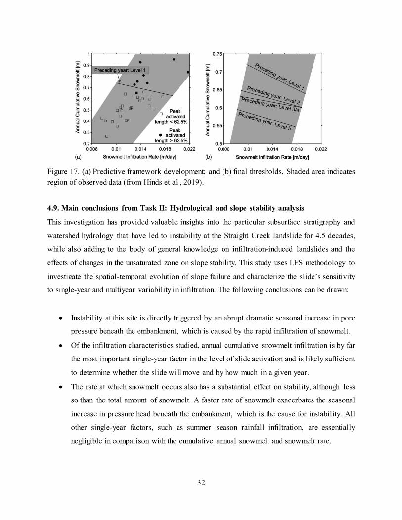
To set these thresholds, each year of available SNOTEL data (1984 through 2017) is modeled
separately, preceded by years of different annual cumulative snowmelt infiltration. These
preceding years were created by multiplying daily infiltration rates for a year of average annual
cumulative snowmelt infiltration (1999) by a factor to match annual cumulative snowmelt
infiltration to the levels specified in Table 4. Level 1 therefore represents a preceding year of

31
minimal annual cumulative snowmelt infiltration, Level 5 a preceding year of maximal annual
cumulative snowmelt infiltration, and Levels 2 through 4 distributed evenly within the observed
range. The resulting activated length is then compared with the minimum activated length
corresponding to pronounced movement, which was set equal to the activated length modeled for
1986 and 2009 when all years were modeled sequentially (as in Figure 12). This is the lowest
activated length modeled for a year of known pronounced movement. The threshold for infiltration
that will likely cause this activated length can then be drawn between model cases that did or did
not exceed it (Figure 17a), disregarding outliers as needed. These thresholds for each level of
annual cumulative snowmelt infiltration in the preceding year can then be combined (Figure 17b).
Predicting snowmelt rate is not as straightforward as predicting annual cumulative snowmelt
infiltration, which can be accurately estimated from SWE values preceding the main snowmelt
season (which typically begins in April or early May). There are no clear correlations between
temperature and snowmelt rate that apply across all years, even controlling for annual cumulative
snowmelt infiltration. However, there are 11 identifiable cases of years with annual cumulative
snowmelt infiltration within 5 mm of each other, nine of which have an identifiable difference in
snowmelt rate. Of the nine cases, eight can be explained by the onset of snowmelt, and nine can
be explained by the average temperature during the 45 days following the onset of snowmelt. Later
onset, closer to early May than mid-April, coincides with high average temperatures in the
subsequent snowmelt season and a faster snowmelt rate. These observations can be used as rough
guides for estimating snowmelt rate, similar to the approach proposed by Chleborad (1998).
Quantifying the Straight Creek slide’s sensitivity to infiltration characteristics may therefore prove
to not only add to the general body of knowledge related to infiltration-induced landslides, but also
to provide practical benefits to CDOT in managing the risks of this slide. Through the use of this
predictive framework, it may be possible to anticipate pronounced movement based on infiltration
in the previous year and predicted annual cumulative snowmelt infiltration and snowmelt
infiltration rate in the current year. This also represents a contribution toward developing hydro-
meteorological thresholds based on the physical processes driving landslide initiation or
reactivation (Bogaard and Greco, 2018; Mirus et al., 2018a, b; Thomas et al., 2018).
32
Figure 17. (a) Predictive framework development; and (b) final thresholds. Shaded area indicates region of observed data (from Hinds et al., 2019).
4.9. Main conclusions from Task II: Hydrological and slope stability analysis
This investigation has provided valuable insights into the particular subsurface stratigraphy and
watershed hydrology that have led to instability at the Straight Creek landslide for 4.5 decades,
while also adding to the body of general knowledge on infiltration-induced landslides and the
effects of changes in the unsaturated zone on slope stability. This study uses LFS methodology to
investigate the spatial-temporal evolution of slope failure and characterize the slide’s sensitivity
to single-year and multiyear variability in infiltration. The following conclusions can be drawn:
• Instability at this site is directly triggered by an abrupt dramatic seasonal increase in pore
pressure beneath the embankment, which is caused by the rapid infiltration of snowmelt.
• Of the infiltration characteristics studied, annual cumulative snowmelt infiltration is by far
the most important single-year factor in the level of slide activation and is likely sufficient
to determine whether the slide will move and by how much in a given year.
• The rate at which snowmelt occurs also has a substantial effect on stability, although less
so than the total amount of snowmelt. A faster rate of snowmelt exacerbates the seasonal
increase in pressure head beneath the embankment, which is the cause for instability. All
other single-year factors, such as summer season rainfall infiltration, are essentially
negligible in comparison with the cumulative annual snowmelt and snowmelt rate.

33
• Slope stability can be affected by infiltration in the previous year. Consecutive years of
high infiltration can have a compounding effect, increasing the magnitude of seasonal
pressure head rise and result in less stability than single, isolated years of high infiltration.
Likewise, consecutive years of low infiltration can suppress groundwater response to
infiltration and increase slope stability in subsequent years. The case study illustrates that
the effects of infiltration characteristics, namely annual snowpack accumulation,
forecasted snowmelt rate, and the previous year’s snowmelt, can be used to form tools for
predicting increased movement of the Straight Creek slide in a given year. This method of
developing instability threshold may be applied to other sites once the physical processes
underlying the evolution of instability are understood.
34
5. TASK III: MITIGATION TECHNIQUES EVALUATION
The contents of this section have been published in Hinds (2018) and Hinds, et al. (2021).
5.1 Objectives
The 2-mile stretch of the I-70 corridor immediately west of the Eisenhower/Johnson Memorial
Tunnels has been the subject of multiple geological investigations due to observed hillslope failures
since the construction of the highway in the late 1960s. At the Straight Creek landslide, two
remediation designs were applied: installing lightweight caissons beneath the highway surface, and
installing horizontal drains near the toe of the landslide.
This task aims to answer the following questions:
a) What were the effects of the lightweight caissons installed in 2011 and 2012?
b) What were the effects of the ten horizontal drains installed in 2012?
c) What would be the potential effects of a proposed drain system installed north of I-70?
5.2 Effect of the lightweight caissons
The caissons were installed by Shannon and Wilson under the westbound lanes in 2011 and under
the median and eastbound lanes in 2012. They are 1.5 m in diameter, 6.1 m deep except under the
middle and right westbound lanes where they are 3 m deep and spaced 3 m on center in seven lines
running parallel to the highway. The unit weight of the lightweight concrete is 5.7 to 6.1 kN/m3
(36 to 39 PCF), in contrast to the estimated unit weight of 21.1 kN/m3 (134 PCF) for the
embankment fill. The volume of all caissons accounts for approximately 1.2% of the total slide
mass volume and approximately 3.1% of the volume of the portion of the slide mass directly
underneath the highway. This represents a weight reduction of 0.9% of the total slide mass and
2.2% of the portion of the slide mass directly underneath the highway. The intent behind the
caisson design was to reduce the driving force, namely gravity, causing the slide, but the total
change in slide mass was relatively modest.
During Phase II of this study, the stability modeling did not find a strong effect on slope stability
from the caissons. Global factor of safety for groundwater levels representative of each season in
the conceptual model were obtained using an extended version of the modified Bishop’s method

35
of slices, which accounts for suction stress as per Lu and Godt (2013), in RocScience Slide 6.0
(Table 7). The effect of the caissons, especially during the most critical summer season, is
negligible in these calculations. This could be because of the small volume of the caissons relative
to the slide mass and to the portion of the slide mass underneath the highway (which are the slices
affected by the caissons in Bishop’s method); it could also be that while the gravitational driving
force was reduced, so was the normal stress on the failure plane under the caissons. This would
reduce the available frictional resistance to movement and counteract the reduction in driving force.
Direct shear testing performed on core samples of the decomposed gneiss, through which the
majority of the failure surface passes, indicates that frictional resistance contributes the majority
of this material’s strength, and it is therefore sensitive to changes in normal force.
Table 6. Effect of caissons on seasonal factor of safety (from Thunder, 2016).
Season Global Factor of Safety
No Caissons With Caissons
Winter 1.05 1.06
Spring 1.05 1.06
Summer 0.95 0.95
Fall 1.04 1.05
However, the caissons could have had other, unexpected effects on the slope. They are not deep
enough to intersect the failure surface, but they could lend structural rigidity to the fill underneath
the highway by resisting deformation. They could have influenced any settlement or consolidation
that was occurring, both by creating vertical stiffness and by reducing overburden driving
consolidation in the embankment below the caissons. This second effect is analogous to the
removal of surcharge used for pre-consolidation of soil under future heavy structures. The soil
directly underneath the caissons would have seen a 14.1% change in vertical stress, possibly
sufficient to reduce consolidation rate dramatically; due to the heterogeneity and spatial variability
of the embankment fill, rigorous analyses of its consolidation behavior are unfortunately not
possible without more extensive field investigation.
5.3 Effects of the horizontal drains near the toe of the slide.
36
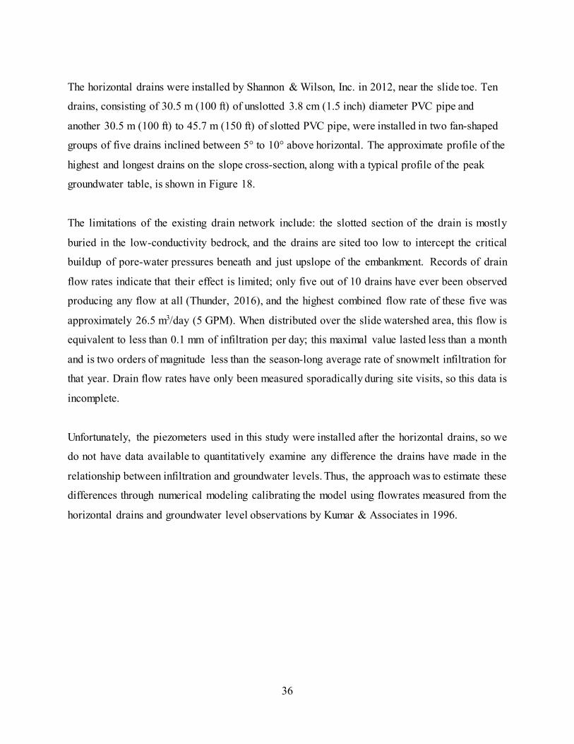
The horizontal drains were installed by Shannon & Wilson, Inc. in 2012, near the slide toe. Ten
drains, consisting of 30.5 m (100 ft) of unslotted 3.8 cm (1.5 inch) diameter PVC pipe and
another 30.5 m (100 ft) to 45.7 m (150 ft) of slotted PVC pipe, were installed in two fan-shaped
groups of five drains inclined between 5° to 10° above horizontal. The approximate profile of the
highest and longest drains on the slope cross-section, along with a typical profile of the peak
groundwater table, is shown in Figure 18.
The limitations of the existing drain network include: the slotted section of the drain is mostly
buried in the low-conductivity bedrock, and the drains are sited too low to intercept the critical
buildup of pore-water pressures beneath and just upslope of the embankment. Records of drain
flow rates indicate that their effect is limited; only five out of 10 drains have ever been observed
producing any flow at all (Thunder, 2016), and the highest combined flow rate of these five was
approximately 26.5 m3/day (5 GPM). When distributed over the slide watershed area, this flow is
equivalent to less than 0.1 mm of infiltration per day; this maximal value lasted less than a month
and is two orders of magnitude less than the season-long average rate of snowmelt infiltration for
that year. Drain flow rates have only been measured sporadically during site visits, so this data is
incomplete.
Unfortunately, the piezometers used in this study were installed after the horizontal drains, so we
do not have data available to quantitatively examine any difference the drains have made in the
relationship between infiltration and groundwater levels. Thus, the approach was to estimate these
differences through numerical modeling calibrating the model using flowrates measured from the
horizontal drains and groundwater level observations by Kumar & Associates in 1996.
37
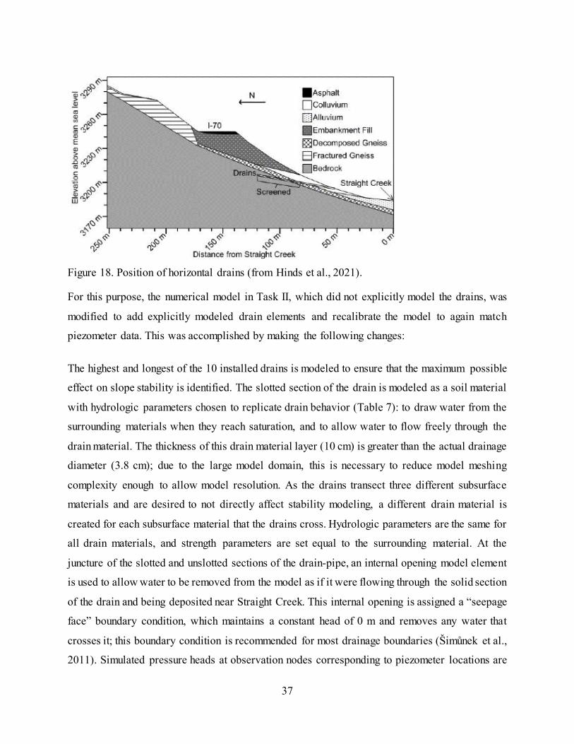
Figure 18. Position of horizontal drains (from Hinds et al., 2021).
For this purpose, the numerical model in Task II, which did not explicitly model the drains, was
modified to add explicitly modeled drain elements and recalibrate the model to again match
piezometer data. This was accomplished by making the following changes:
The highest and longest of the 10 installed drains is modeled to ensure that the maximum possible
effect on slope stability is identified. The slotted section of the drain is modeled as a soil material
with hydrologic parameters chosen to replicate drain behavior (Table 7): to draw water from the
surrounding materials when they reach saturation, and to allow water to flow freely through the
drain material. The thickness of this drain material layer (10 cm) is greater than the actual drainage
diameter (3.8 cm); due to the large model domain, this is necessary to reduce model meshing
complexity enough to allow model resolution. As the drains transect three different subsurface
materials and are desired to not directly affect stability modeling, a different drain material is
created for each subsurface material that the drains cross. Hydrologic parameters are the same for
all drain materials, and strength parameters are set equal to the surrounding material. At the
juncture of the slotted and unslotted sections of the drain-pipe, an internal opening model element
is used to allow water to be removed from the model as if it were flowing through the solid section
of the drain and being deposited near Straight Creek. This internal opening is assigned a “seepage
face” boundary condition, which maintains a constant head of 0 m and removes any water that
crosses it; this boundary condition is recommended for most drainage boundaries (Šimůnek et al.,
2011). Simulated pressure heads at observation nodes corresponding to piezometer locations are
38
generated using daily SNOTEL infiltration data for the years over which piezometer data are
available; material hydrologic properties and spatial distribution are then calibrated within ranges
constrained by literature, previous laboratory testing programs, and interpretation of borehole logs
to match observed piezometer data and drain fluxes as closely as possible.
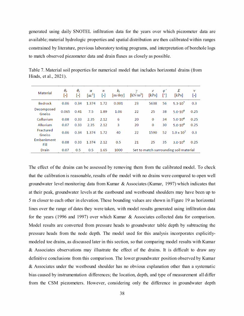
Table 7. Material soil properties for numerical model that includes horizontal drains (from Hinds, et al., 2021).
The effect of the drains can be assessed by removing them from the calibrated model. To check
that the calibration is reasonable, results of the model with no drains were compared to open well
groundwater level monitoring data from Kumar & Associates (Kumar, 1997) which indicates that
at their peak, groundwater levels at the eastbound and westbound shoulders may have been up to
5 m closer to each other in elevation. These bounding values are shown in Figure 19 as horizontal
lines over the range of dates they were taken, with model results generated using infiltration data
for the years (1996 and 1997) over which Kumar & Associates collected data for comparison.
Model results are converted from pressure heads to groundwater table depth by subtracting the
pressure heads from the node depth. The model used for this analysis incorporates explicitly-
modeled toe drains, as discussed later in this section, so that comparing model results with Kumar
& Associates observations may illustrate the effect of the drains. It is difficult to draw any
definitive conclusions from this comparison. The lower groundwater position observed by Kumar
& Associates under the westbound shoulder has no obvious explanation other than a systematic
bias caused by instrumentation differences; the location, depth, and type of measurement all differ
from the CSM piezometers. However, considering only the difference in groundwater depth
39
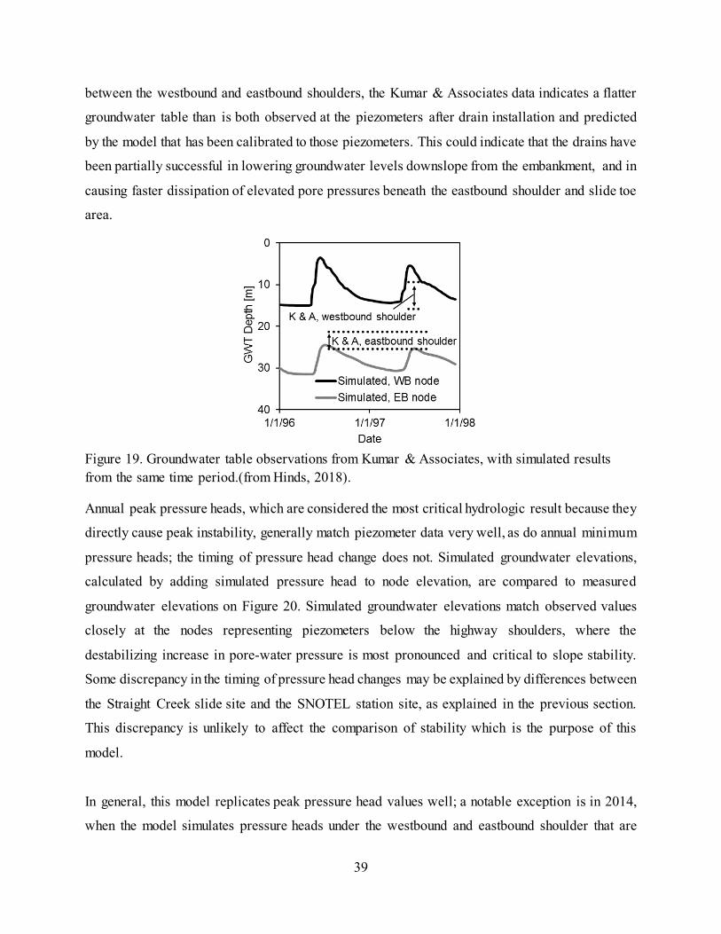
between the westbound and eastbound shoulders, the Kumar & Associates data indicates a flatter
groundwater table than is both observed at the piezometers after drain installation and predicted
by the model that has been calibrated to those piezometers. This could indicate that the drains have
been partially successful in lowering groundwater levels downslope from the embankment, and in
causing faster dissipation of elevated pore pressures beneath the eastbound shoulder and slide toe
area.
Figure 19. Groundwater table observations from Kumar & Associates, with simulated results from the same time period.(from Hinds, 2018).
Annual peak pressure heads, which are considered the most critical hydrologic result because they
directly cause peak instability, generally match piezometer data very well, as do annual minimum
pressure heads; the timing of pressure head change does not. Simulated groundwater elevations,
calculated by adding simulated pressure head to node elevation, are compared to measured
groundwater elevations on Figure 20. Simulated groundwater elevations match observed values
closely at the nodes representing piezometers below the highway shoulders, where the
destabilizing increase in pore-water pressure is most pronounced and critical to slope stability.
Some discrepancy in the timing of pressure head changes may be explained by differences between
the Straight Creek slide site and the SNOTEL station site, as explained in the previous section.
This discrepancy is unlikely to affect the comparison of stability which is the purpose of this
model.
In general, this model replicates peak pressure head values well; a notable exception is in 2014,
when the model simulates pressure heads under the westbound and eastbound shoulder that are
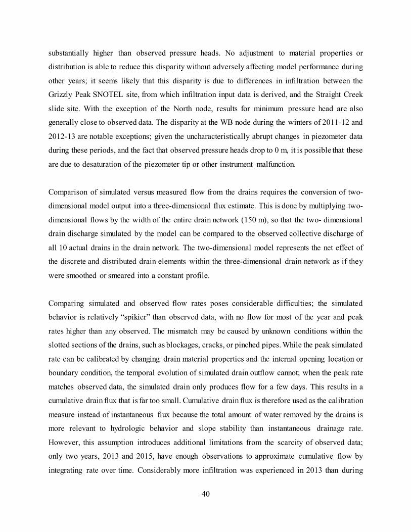
40
substantially higher than observed pressure heads. No adjustment to material properties or
distribution is able to reduce this disparity without adversely affecting model performance during
other years; it seems likely that this disparity is due to differences in infiltration between the
Grizzly Peak SNOTEL site, from which infiltration input data is derived, and the Straight Creek
slide site. With the exception of the North node, results for minimum pressure head are also
generally close to observed data. The disparity at the WB node during the winters of 2011-12 and
2012-13 are notable exceptions; given the uncharacteristically abrupt changes in piezometer data
during these periods, and the fact that observed pressure heads drop to 0 m, it is possible that these
are due to desaturation of the piezometer tip or other instrument malfunction.
Comparison of simulated versus measured flow from the drains requires the conversion of two-
dimensional model output into a three-dimensional flux estimate. This is done by multiplying two-
dimensional flows by the width of the entire drain network (150 m), so that the two- dimensional
drain discharge simulated by the model can be compared to the observed collective discharge of
all 10 actual drains in the drain network. The two-dimensional model represents the net effect of
the discrete and distributed drain elements within the three-dimensional drain network as if they
were smoothed or smeared into a constant profile.
Comparing simulated and observed flow rates poses considerable difficulties; the simulated
behavior is relatively “spikier” than observed data, with no flow for most of the year and peak
rates higher than any observed. The mismatch may be caused by unknown conditions within the
slotted sections of the drains, such as blockages, cracks, or pinched pipes. While the peak simulated
rate can be calibrated by changing drain material properties and the internal opening location or
boundary condition, the temporal evolution of simulated drain outflow cannot; when the peak rate
matches observed data, the simulated drain only produces flow for a few days. This results in a
cumulative drain flux that is far too small. Cumulative drain flux is therefore used as the calibration
measure instead of instantaneous flux because the total amount of water removed by the drains is
more relevant to hydrologic behavior and slope stability than instantaneous drainage rate.
However, this assumption introduces additional limitations from the scarcity of observed data;
only two years, 2013 and 2015, have enough observations to approximate cumulative flow by
integrating rate over time. Considerably more infiltration was experienced in 2013 than during
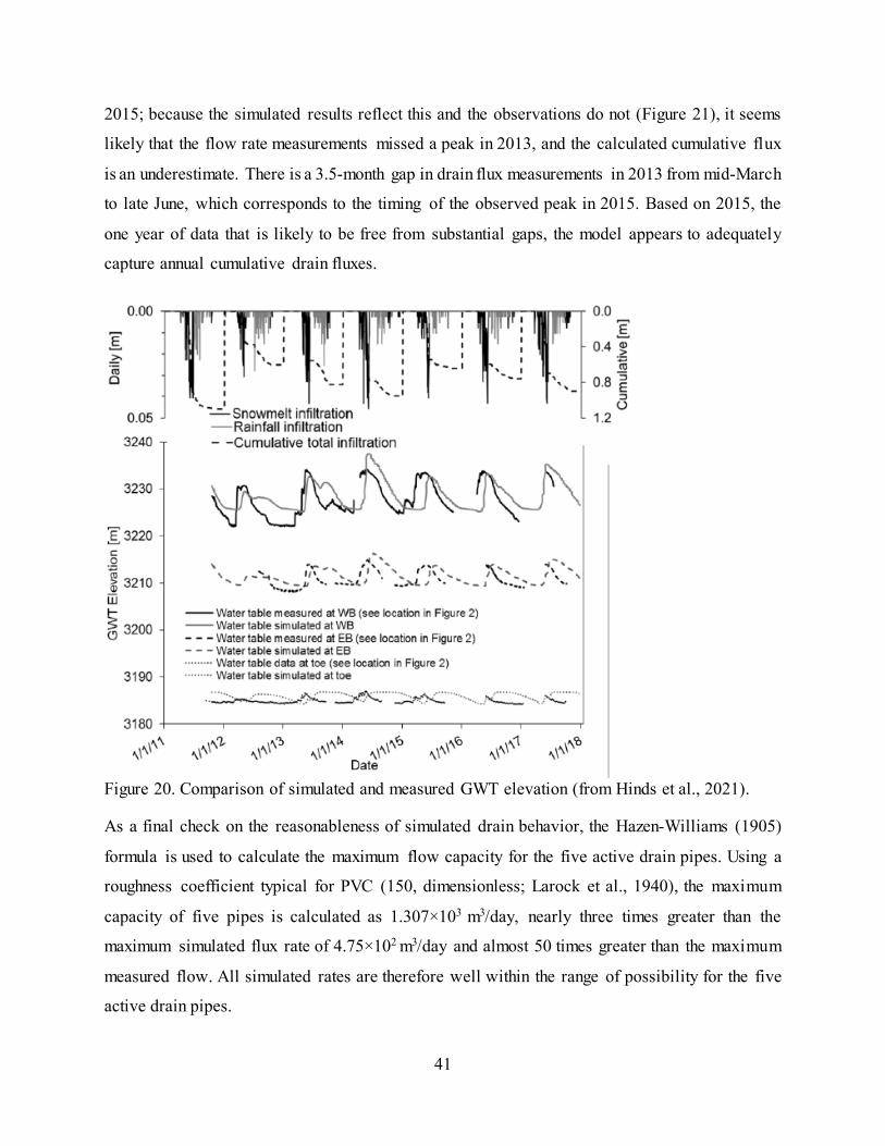
41
2015; because the simulated results reflect this and the observations do not (Figure 21), it seems
likely that the flow rate measurements missed a peak in 2013, and the calculated cumulative flux
is an underestimate. There is a 3.5-month gap in drain flux measurements in 2013 from mid-March
to late June, which corresponds to the timing of the observed peak in 2015. Based on 2015, the
one year of data that is likely to be free from substantial gaps, the model appears to adequately
capture annual cumulative drain fluxes.
Figure 20. Comparison of simulated and measured GWT elevation (from Hinds et al., 2021).
As a final check on the reasonableness of simulated drain behavior, the Hazen-Williams (1905)
formula is used to calculate the maximum flow capacity for the five active drain pipes. Using a
roughness coefficient typical for PVC (150, dimensionless; Larock et al., 1940), the maximum
capacity of five pipes is calculated as 1.307×10³ m3/day, nearly three times greater than the
maximum simulated flux rate of 4.75×10² m3/day and almost 50 times greater than the maximum
measured flow. All simulated rates are therefore well within the range of possibility for the five
active drain pipes.
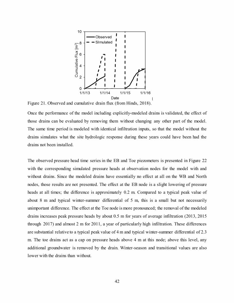
42
Figure 21. Observed and cumulative drain flux (from Hinds, 2018).
Once the performance of the model including explicitly-modeled drains is validated, the effect of
those drains can be evaluated by removing them without changing any other part of the model.
The same time period is modeled with identical infiltration inputs, so that the model without the
drains simulates what the site hydrologic response during these years could have been had the
drains not been installed.
The observed pressure head time series in the EB and Toe piezometers is presented in Figure 22
with the corresponding simulated pressure heads at observation nodes for the model with and
without drains. Since the modeled drains have essentially no effect at all on the WB and North
nodes, those results are not presented. The effect at the EB node is a slight lowering of pressure
heads at all times; the difference is approximately 0.2 m. Compared to a typical peak value of
about 8 m and typical winter-summer differential of 5 m, this is a small but not necessarily
unimportant difference. The effect at the Toe node is more pronounced; the removal of the modeled
drains increases peak pressure heads by about 0.5 m for years of average infiltration (2013, 2015
through 2017) and almost 2 m for 2011, a year of particularly high infiltration. These differences
are substantial relative to a typical peak value of 4 m and typical winter-summer differential of 2.3
m. The toe drains act as a cap on pressure heads above 4 m at this node; above this level, any
additional groundwater is removed by the drain. Winter-season and transitional values are also
lower with the drains than without.
43
Figure 22. Observed and simulated (with and without toe drains) pressure heads at the EB and Toe nodes.(from Hinds, 2018).
Slope Cube results indicate that the drains’ effect on hydrology also influences slope stability, as
expected. LFS contour plots of the model with and without toe drains at the same model time
step show this effect (Figure 23). This time step corresponds roughly to July 30, 2011, the least
stable point in time for the modeled period (2011 through 2018, the period of piezometer data
availability). The main difference is in the area directly above and below the drains, where the
lower pore pressures enforced by the drains create a gap in the otherwise continuous band of LFS
this point in time, although the width of the band of LFS < 1 is also reduced by the drains in the
toe area. For this point in time, the difference in activated length (portion of failure surface where
LFS < 1) is 2.2% of the full failure surface.
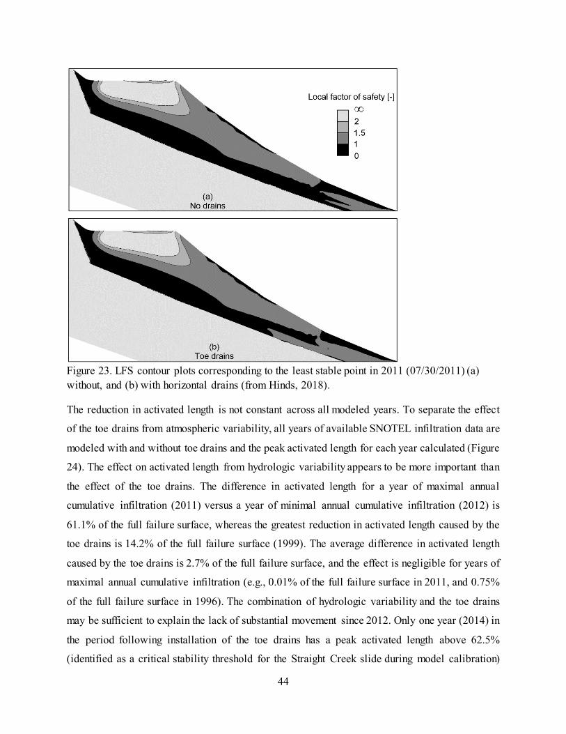
44
Figure 23. LFS contour plots corresponding to the least stable point in 2011 (07/30/2011) (a) without, and (b) with horizontal drains (from Hinds, 2018).
The reduction in activated length is not constant across all modeled years. To separate the effect
of the toe drains from atmospheric variability, all years of available SNOTEL infiltration data are
modeled with and without toe drains and the peak activated length for each year calculated (Figure
24). The effect on activated length from hydrologic variability appears to be more important than
the effect of the toe drains. The difference in activated length for a year of maximal annual
cumulative infiltration (2011) versus a year of minimal annual cumulative infiltration (2012) is
61.1% of the full failure surface, whereas the greatest reduction in activated length caused by the
toe drains is 14.2% of the full failure surface (1999). The average difference in activated length
caused by the toe drains is 2.7% of the full failure surface, and the effect is negligible for years of
maximal annual cumulative infiltration (e.g., 0.01% of the full failure surface in 2011, and 0.75%
of the full failure surface in 1996). The combination of hydrologic variability and the toe drains
may be sufficient to explain the lack of substantial movement since 2012. Only one year (2014) in
the period following installation of the toe drains has a peak activated length above 62.5%
(identified as a critical stability threshold for the Straight Creek slide during model calibration)
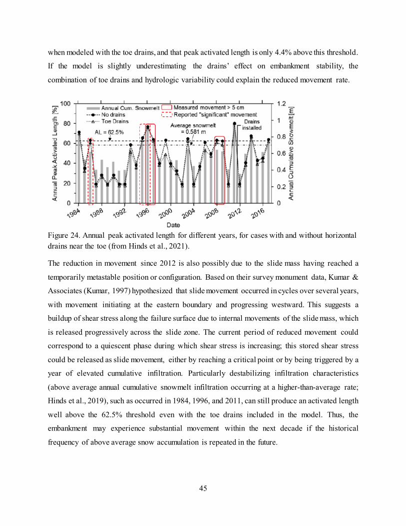
45
when modeled with the toe drains, and that peak activated length is only 4.4% above this threshold.
If the model is slightly underestimating the drains’ effect on embankment stability, the
combination of toe drains and hydrologic variability could explain the reduced movement rate.
Figure 24. Annual peak activated length for different years, for cases with and without horizontal drains near the toe (from Hinds et al., 2021).
The reduction in movement since 2012 is also possibly due to the slide mass having reached a
temporarily metastable position or configuration. Based on their survey monument data, Kumar &
Associates (Kumar, 1997) hypothesized that slide movement occurred in cycles over several years,
with movement initiating at the eastern boundary and progressing westward. This suggests a
buildup of shear stress along the failure surface due to internal movements of the slide mass, which
is released progressively across the slide zone. The current period of reduced movement could
correspond to a quiescent phase during which shear stress is increasing; this stored shear stress
could be released as slide movement, either by reaching a critical point or by being triggered by a
year of elevated cumulative infiltration. Particularly destabilizing infiltration characteristics
(above average annual cumulative snowmelt infiltration occurring at a higher-than-average rate;
Hinds et al., 2019), such as occurred in 1984, 1996, and 2011, can still produce an activated length
well above the 62.5% threshold even with the toe drains included in the model. Thus, the
embankment may experience substantial movement within the next decade if the historical
frequency of above average snow accumulation is repeated in the future.
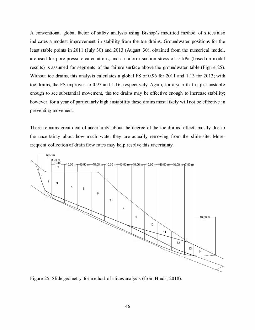
46
A conventional global factor of safety analysis using Bishop’s modified method of slices also
indicates a modest improvement in stability from the toe drains. Groundwater positions for the
least stable points in 2011 (July 30) and 2013 (August 30), obtained from the numerical model,
are used for pore pressure calculations, and a uniform suction stress of -5 kPa (based on model
results) is assumed for segments of the failure surface above the groundwater table (Figure 25).
Without toe drains, this analysis calculates a global FS of 0.96 for 2011 and 1.13 for 2013; with
toe drains, the FS improves to 0.97 and 1.16, respectively. Again, for a year that is just unstable
enough to see substantial movement, the toe drains may be effective enough to increase stability;
however, for a year of particularly high instability these drains most likely will not be effective in
preventing movement.
There remains great deal of uncertainty about the degree of the toe drains’ effect, mostly due to
the uncertainty about how much water they are actually removing from the slide site. More-
frequent collection of drain flow rates may help resolve this uncertainty.
Figure 25. Slide geometry for method of slices analysis (from Hinds, 2018).
47
6. TASK IV: EVALUATION OF DRAIN SYSTEM NORTH OF I-70 While the existing toe drains had a modest effect improving the site drainage and stability, the
insights gained through the three phases of this investigation indicate that a remediation approach
targeting the primary driver of slope movement could have a greater impact. The hydrology of the
Straight Creek slide creates a very specific failure mechanism, which can be specifically addressed
to maximize the impact of remediation work. Based on modeling results, the main cause of this
slide is the infiltration of snowmelt on the northern slope above the highway, which flows rapidly
downslope until it hits the sharp contrast in hydraulic conductivity created by the decomposed
gneiss and embankment material. The resulting spike in pore pressures directly causes the seasonal
loss of stability that has led to recurring slide movement over the majority of the embankment’s
service life. If the backup of groundwater is prevented from happening in the first place, the slide
could be stabilized more effectively.
One feasible approach to achieve this is to install a drain system in the north slope, above the
westbound shoulder of I-70 (Figure 26). A limiting factor on the location of the toe drain system
was drill rig access; installing the drains any higher up would have required getting a rig up the
increasingly steep, topographically rugged slope, which is covered in loose talus and colluvium
and closely spaced trees. Drains extending into the north slope could be drilled from the 11 m wide,
flat, paved westbound shoulder, with easy access for machinery, supplies, and personnel.
The preliminary design considered here consists of 12 drains in four fanned groups of three, spaced
at even intervals of about 50 m along the side of I-70, projecting perpendicularly from the
westbound shoulder of the highway at a pitch of 10°. The drains would consist of similar PVC
pipe as the toe drains, extending the same distance (70 m) past the surface. Modeling of these
drains suggests that a longer slotted section is desirable, with only the final 15 m consisting of
solid pipe; this would allow for as much water to be removed from the shallow subsurface as
possible. The drains would empty into a culvert running parallel to the westbound shoulder to carry
water downslope to the lined Harrison Gulch culvert approximately 680 m to the west, which
already runs underneath the highway towards Straight Creek.
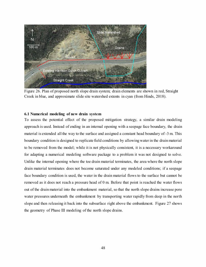
48
Figure 26. Plan of proposed north slope drain system; drain elements are shown in red, Straight Creek in blue, and approximate slide site watershed extents in cyan (from Hinds, 2018).
6.1 Numerical modeling of new drain system To assess the potential effect of the proposed mitigation strategy, a similar drain modeling
approach is used. Instead of ending in an internal opening with a seepage face boundary, the drain
material is extended all the way to the surface and assigned a constant head boundary of -3 m. This
boundary condition is designed to replicate field conditions by allowing water in the drain material
to be removed from the model; while it is not physically consistent, it is a necessary workaround
for adapting a numerical modeling software package to a problem it was not designed to solve.
Unlike the internal opening where the toe drain material terminates, the area where the north slope
drain material terminates does not become saturated under any modeled conditions; if a seepage
face boundary condition is used, the water in the drain material flows to the surface but cannot be
removed as it does not reach a pressure head of 0 m. Before that point is reached the water flows
out of the drain material into the embankment material, so that the north slope drains increase pore
water pressures underneath the embankment by transporting water rapidly from deep in the north
slope and then releasing it back into the subsurface right above the embankment. Figure 27 shows
the geometry of Phase III modeling of the north slope drains.
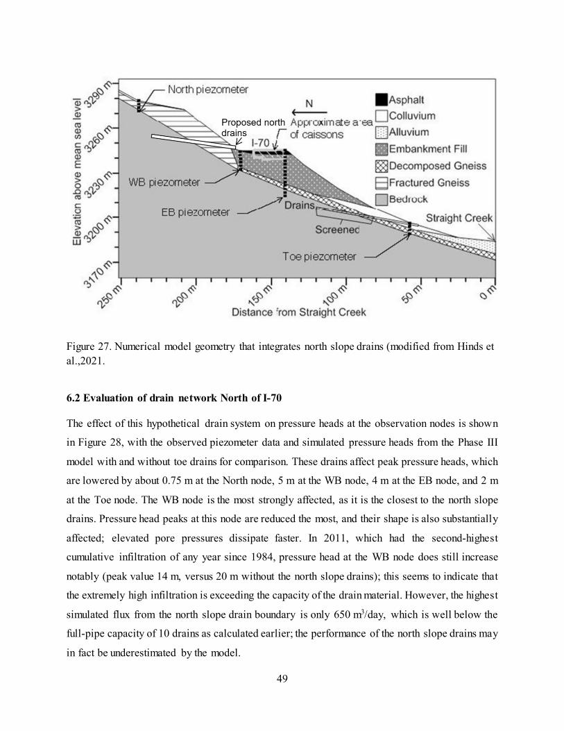
49
Figure 27. Numerical model geometry that integrates north slope drains (modified from Hinds et al.,2021.
6.2 Evaluation of drain network North of I-70 The effect of this hypothetical drain system on pressure heads at the observation nodes is shown
in Figure 28, with the observed piezometer data and simulated pressure heads from the Phase III
model with and without toe drains for comparison. These drains affect peak pressure heads, which
are lowered by about 0.75 m at the North node, 5 m at the WB node, 4 m at the EB node, and 2 m
at the Toe node. The WB node is the most strongly affected, as it is the closest to the north slope
drains. Pressure head peaks at this node are reduced the most, and their shape is also substantially
affected; elevated pore pressures dissipate faster. In 2011, which had the second-highest
cumulative infiltration of any year since 1984, pressure head at the WB node does still increase
notably (peak value 14 m, versus 20 m without the north slope drains); this seems to indicate that
the extremely high infiltration is exceeding the capacity of the drain material. However, the highest
simulated flux from the north slope drain boundary is only 650 m3/day, which is well below the
full-pipe capacity of 10 drains as calculated earlier; the performance of the north slope drains may
in fact be underestimated by the model.
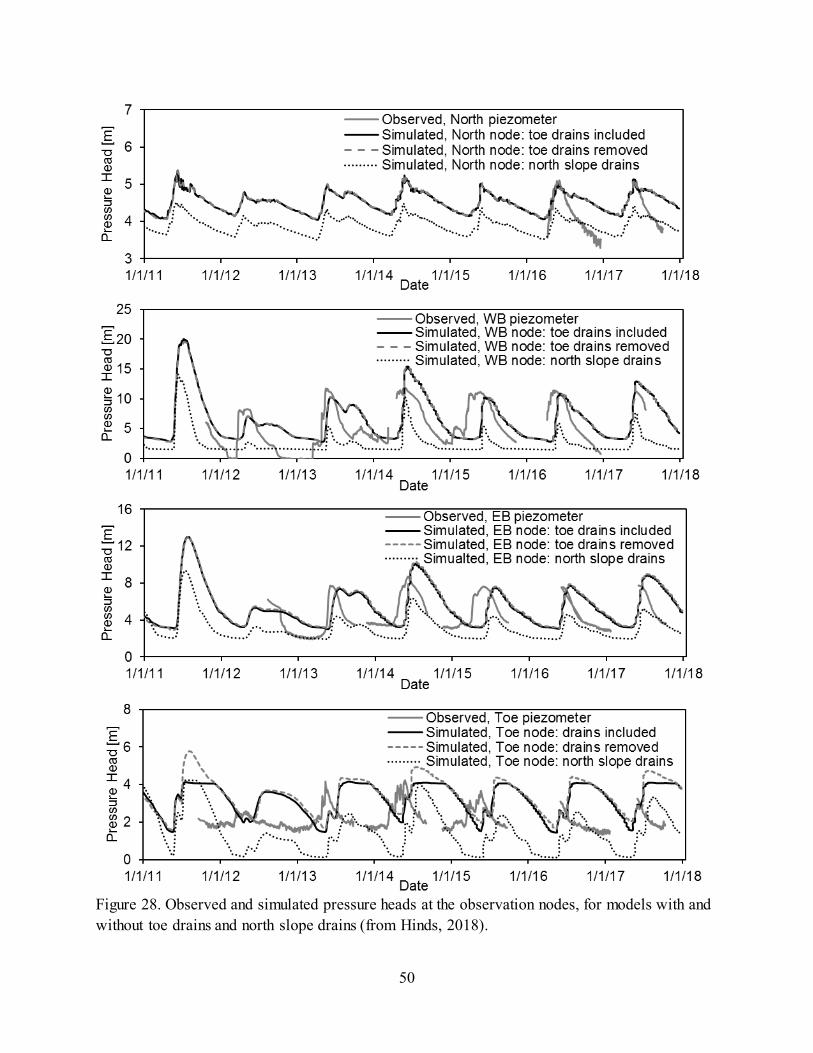
50
Figure 28. Observed and simulated pressure heads at the observation nodes, for models with and without toe drains and north slope drains (from Hinds, 2018).
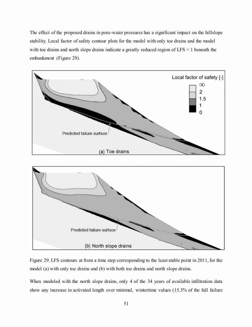
51
The effect of the proposed drains in pore-water pressures has a significant impact on the hillslope
stability. Local factor of safety contour plots for the model with only toe drains and the model
with toe drains and north slope drains indicate a greatly reduced region of LFS < 1 beneath the
embankment (Figure 29).
Figure 29. LFS contours at from a time step corresponding to the least stable point in 2011, for the
model (a) with only toe drains and (b) with both toe drains and north slope drains.
When modeled with the north slope drains, only 4 of the 34 years of available infiltration data
show any increase in activated length over minimal, wintertime values (15.3% of the full failure

52
surface). Annual peak activated lengths calculated over the period of available infiltration data
illustrate that the effect of the north slope drains could result in a substantial improvement in
stability (Figure 30). No year modeled with the north slope drains has a peak activated length
above the 62.5% threshold, which was the lowest peak activated length for a year of known
increased movement. Only 2011, the year of highest annual cumulative infiltration, has an
activated length above 40% of the full failure surface. The toe drains reduce peak activated length
by an average value of 2.7% of the full failure surface when compared to the model without any
drains; the north slope drains reduce peak activated length by an average value of 24.8% of the
full failure surface when compared to the toe drains, a more substantial improvement in predicted
stability.
Conventional global FS analyses using Bishop’s modified method of slices also indicate that the
north slope drains could be more effective than past remediation techniques. Groundwater
positions for the least stable points in 2011 (July 21) and 2013 (July 10), derived from model
results, are used for pore-water pressure calculations, and a uniform suction stress of -5 kPa is
assumed for segments of the failure surface above the groundwater table. For the least stable point
in 2011, the global FS without any drains is 11% smaller than the FS with north slope drains, and
in 2013, the FS without drains is 8.6% smaller than the FS with north slope drains. Thus, the north
slope drains are more effective in eliminating progressive failure and small slide movements in
years of average infiltration.
The proposed north slope drains network is just one possible effective remediation. They have the
potential to substantially change the stability of the Straight Creek slide, possibly eliminating slide
movement altogether. They could accomplish this for a smaller cost than has already been spent
on remediation for this site, eliminate the expenditure on annual asphalt capping operations that
are currently necessary to maintain roadway serviceability, and not require any traffic lane
closures. We conclude that a Phase IV study to engineer an optimum upslope drain system would
result in a long-term solution to the Straight Creek slide problem.
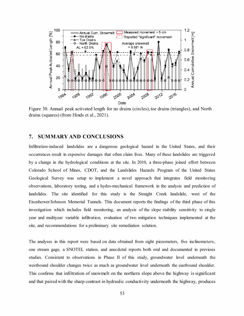
53
Figure 30. Annual peak activated length for no drains (circles), toe drains (triangles), and North drains (squares) (from Hinds et al., 2021).
7. SUMMARY AND CONCLUSIONS
Infiltration-induced landslides are a dangerous geological hazard in the United States, and their
occurrences result in expensive damages that often claim lives. Many of these landslides are triggered
by a change in the hydrological conditions at the site. In 2010, a three-phase joined effort between
Colorado School of Mines, CDOT, and the Landslides Hazards Program of the United States
Geological Survey was setup to implement a novel approach that integrates field monitoring
observations, laboratory testing, and a hydro-mechanical framework in the analysis and prediction of
landslides. The site identified for this study is the Straight Creek landslide, west of the
Eisenhower/Johnson Memorial Tunnels. This document reports the findings of the third phase of this
investigation which includes field monitoring, an analysis of the slope stability sensitivity to single
year and multiyear variable infiltration, evaluation of two mitigation techniques implemented at the
site, and recommendations for a preliminary site remediation solution.
The analyses in this report were based on data obtained from eight piezometers, five inclinometers,
one stream gage, a SNOTEL station, and anecdotal reports both oral and documented in previous
studies. Consistent to observations in Phase II of this study, groundwater level underneath the
westbound shoulder changes twice as much as groundwater level underneath the eastbound shoulder.
This confirms that infiltration of snowmelt on the northern slope above the highway is significant
and that paired with the sharp contrast in hydraulic conductivity underneath the highway, produces

54
a peak in pore water pressures and affects the stability of the hillslope. Based on older and newer
inclinometer readings, field observations, and numerical analysis results, the failure plane of the
landslide is believed to start near the westbound shoulder of I-70 and run along the decomposed
gneiss-bedrock interface.
From the spatiotemporal evolution analysis of slope failure due to changes in the hydrology of the
hillslope, the following conclusions are drawn:
• Instability at this site is directly triggered by an abrupt dramatic seasonal increase in pore
pressure beneath the embankment, which is caused by the rapid infiltration of snowmelt.
• Slope stability is sensitive to annual cumulative snowmelt infiltration and rate at which
snowmelt occurs. Of the infiltration characteristics studied, annual cumulative snowmelt
infiltration is by far the most important single-year factor in the level of slide activation
and is likely sufficient to determine whether the slide will move and by how much in a
given year. The rate at which snowmelt occurs also has a substantial effect on stability,
although less so than the total amount of snowmelt. A faster rate of snowmelt exacerbates
the seasonal increase in pressure head beneath the embankment, which is the cause for
instability.
• Slope stability can be affected by infiltration in the previous year. Consecutive years of
high infiltration can have a compounding effect, increasing the magnitude of seasonal
pressure head rise and resulting in less stability than single, isolated years of high
infiltration. Likewise, consecutive years of low infiltration can suppress groundwater
response to infiltration and increase slope stability in subsequent years.
• Smaller movements in the last five years may be explained by the combination of
cumulative snowmelt infiltration, snowmelt infiltration rate, and infiltration in previous
years.
From the evaluation of the effect of lightweight caissons and horizontal drains installed at the site
in 2011 and 2012, the following conclusions can be drawn:

55
• The use of lightweight caissons to reduce the slide mass was minimally effective. The
caissons reduced weight of the slide mass by 0.9%, which translated in a change in FOS of
less than 1%. Remediation techniques that address the pore water pressure are more
effective.
• The installation of horizontal drains near the slide toe had a modest effect on site stability.
Pore pressures are only reduced in a localized area near the drains, but due to the low
hydraulic conductivity of the embankment materials, it is ineffective beneath the
embankment.
• The drains may have been sufficient to stabilize the embankment during the period of low
to average annual cumulative infiltration, but not for years of higher annual cumulative
infiltration.
Based on the results of this study, the main cause of this slide is the infiltration of snowmelt on the
northern slope above the highway, which flows rapidly downslope until it hits the sharp contrast
in hydraulic conductivity created by the decomposed gneiss and embankment material. Thus, we
conclude that a remediation solution could be engineered to prevent large increases in pore water
pressures north of I-70. One preliminary design is a 12 horizontal drains network north of I-70; for
such a system, the numerical analysis indicates:
• The seasonal reduction of stability at the Straight Creek slide is eliminated, even for years
of higher annual cumulative infiltration. This is a significant improvement compared to the
minimal effect on factor of safety of the installation of lightweight caissons.
• A critical threshold for slide movement under conditions similar to years 1984-2018 is not
crossed.
• The proposed drains intercept upslope flow before the hydraulic conductivity contrast at
the embankment; therefore, the intercepted flow could be safely diverted away from the
embankment.
• The proposed remediation has easier access for equipment and personnel.
56
8. FURTHER ACTIONS
Based on all the data obtained from previous reports and during the past three phases of this study,
it is clear that the main cause of this slide is the infiltration of snowmelt on the northern slope
above the highway. This large infiltration through decomposed gneiss, paired with a sharp contrast
in hydraulic conductivity of materials underneath the highway, results in an increase of pore water
pressures and a decrease in the stability of the slope. Thus, we conclude that a remediation solution
could be engineered to prevent large increases in pore water pressures north of I-70. The analyzed
preliminary design for a drainage system provides encouraging results. A Phase IV: Study and
Engineer of Optimum Upslope Drain System would be needed to adequately optimize the long-
term solution of the study site. This new study could include:
• Numerical analyses of other drain configurations to find the most effective alternative.
• Installation of proposed drain system.
• Monitoring of drain system, groundwater table, and stability of hillslope.
57
9. REFERENCES
Bogaard, T. and Greco, R. (2018). “Invited perspectives: A hydrological look to precipitation
intensity duration thresholds for landslide initiation: Proposing hydro-meteorological thresholds.”
Natural Hazards and Earth System Science, 18(1): 31–39. https://doi.org/10.5194/nhess-18-31-
2018
Campbell, R. H. (1975). “Soil slip, debris flows, and rainstorms in the Santa Monica Mountains
and vicinity, southern California.” U.S. Geological Survey Professional Paper 851, 58 pp.
https://doi.org/10.3133/pp851
Chleborad, A. F. (1998). “Use of air temperature to anticipate the onset of snowmelt season
landslides.” U.S. Geological Survey Open File Report 98-124, 17 pp.
https://doi.org/10.3133/ofr98124
Hinds, E. (2018). Effects of atmospheric variability and remediation techniques on the stability of
an interstate highway embankment. M.S. Thesis, Colorado School of Mines: Golden, CO, 167 pp.
https://hdl.handle.net/11124/172344
Hinds, E., Lu, N., Mirus, B., Wayllace, A. (2019). “Effects of Infiltration Characteristics on
Spatial-Temporal Evolution of Stability of an Interstate Highway Embankment.” Journal of
Geotechnical and Geoenvironmental Engineering, 145(9): 05019008.
https://doi.org/10.1061/(ASCE)GT.1943-5606.0002127
Hinds, E. S., Lu, N., Mirus, B. B., Godt, J. W., & Wayllace, A. (2021). Evaluation of techniques
for mitigating snowmelt infiltration-induced landsliding in a highway embankment. Engineering
Geology, 106240.
Kumar & Associates. (1997). Progress report of geological and geotechnical data acquisition,
embankment slope instability study, Straight Creek, Interstate-70 west of Eisenhower Tunnel,
Summit County, Colorado.
Lim, K., Engel, B., Tang, Z., Choi, J., Kim, K., Muthukrishnan, S., and Tripathy, D. (2005).
“Automated web GIS based hydrograph tool, WHAT.” Journal of the American Water Resources
Association, 41(6): 1407–1416. https://doi.org/10.1111/j.1752-1688.2005.tb03808.x
58
Lu, N., and LeCain, G. (2003). “Percolation induced heat transfer in deep unsaturated zones.”
Journal of Geotechnical and Geoenvironmental Engineering, 129(11): 1040–1053.
https://doi.org/10.1061/(ASCE)1090-0241(2003)129:11(1040)
Lu, N., and Likos, W.J. (2004). Unsaturated Soil Mechanics, John Wiley and Sons.
Lu, N., and Likos, W. J. (2006). "Suction stress characteristic curve for unsaturated soils," Journal
of Geotechnical and Geoenvironmental Engineering, Vol. 132(2), 131–142.
Lu, N., (2008). “Is matric suction a stress variable?” Journal of Geotechnical and
Geoenvironmental Engineering, Vol. 134(7), 899-905.
Lu, N., & Godt, J. W. (2013). Hillslope hydrology and stability. Cambridge University Press.
Lu, N., Godt, J. W., and Wu, D. T. (2010). “A closed‐form equation for effective stress in
unsaturated soil,” Water Resources Research, Vol. 46(5).
Lu, N., Wayllace, A., and Oh, S. (2013). “Infiltration-induced seasonally reactivated instability of
a highway embankment near the Eisenhower Tunnel, Colorado, USA.” Engineering Geology, 162:
22–32. https://doi.org/10.1016/j.enggeo.2013.05.002
Lu, N., Wayllace, A., and Formetta, G. (2016). The Slope Cube Module for HYDRUS (2D):
Simulating Slope Stress and Stability in Variably-Saturated Hillslopes, Technical Manual, Version
1.0, Soil Water Retention LLC.
Mirus, B. B., Becker, R. E., Baum, R. L., and Smith, J. B. (2018a). “Integrating real-time
subsurface hydrologic monitoring with empirical rainfall thresholds to improve landslide early
warning.” Landslides, 15(10): 1909–1919. https://doi.org/10.1007/s10346-018-0995-z
Mirus, B. B., Morphew, M. D., and Smith, J. B. (2018b). “Developing hydro-meteorological
thresholds for shallow landslide initiation and early warning.” Water, 10(9): 1274.
https://doi.org/10.3390/w10091274
59
Mualem, Y. (1976). “A new model for predicting the hydraulic conductivity of unsaturated porous
media,” Water Resources Research, 12(3), 513-522.
Nathan, R. and McMahon, T. (1990). “Evaluation of automated techniques for base flow and
recession analyses.” Water Resources Research, 26(7): 1465–1473.
https://doi.org/10.1029/WR026i007p01465
NRCS (2018). “Colorado SNOTEL Site Number 505 Grizzly Peak.” United States Department of
Agriculture, Natural Resources Conservation Service.
https://wcc.sc.egov.usda.gov/nwcc/site?sitenum=505
Richards, L. (1931). “Capillary conduction of liquids through porous mediums,” Journal of
Applied Physics, Vol. 316.
Šimůnek, J., van Genuchten, M. Th., and Šejna, M. (2011). The HYDRUS Software Package for
Simulating Two- and Three-Dimensional Movement of Water, Heat, and Multiple Solutes in
Variably-Saturated Media, Technical Manual, Version 2.0, PC Progress SRO.
Thomas, M. A., Mirus, B. B., Collins, B. D., Lu, N., and Godt, J. W. (2018). Variability in soil-
water retention properties and implications for physics-based simulation of landslide early warning
criteria: Landslides. https://doi.org/10.1007/s10346-018-0950-z
Thunder, B. (2016). The Hydro-mechanical Analysis of an Infiltration-Induced Landslide Along
I-70 in Summit County, CO. Master’s Thesis, Colorado School of Mines: Golden, CO, 83 pp.
http://hdl.handle.net/11124/170303
USGS (2018). “USGS Stream Gage 09051050: Straight Creek below Laskey Gulch near Dillon,
CO.” U.S. Geological Survey, National Water Information System.
https://waterdata.usgs.gov/monitoring-location/09051050/
USGS StreamStats (2018). “StreamStats: Streamflow Statistics and Spatial Analysis Tools for
Water-Resources Applications, Version 4.2.0.” U.S. Geological Survey, Web Informatics and
Mapping Team. https://streamstats.usgs.gov/
60
van Genuchten, M. Th. (1980). “A closed form equation for predicting the hydraulic conductivity
of unsaturated soils,” Soil Science Society of American Journal, Vol. 44, 892-898.
Wayllace, A., Lu, N., Oh, S., and Thomas, D. (2012). “Perennial infiltration-induced instability of
Interstate-70 embankment west of the Eisenhower/Johnson Memorial Tunnels.” In Hryciw, R. D.,
Athanasopoulos-Zekkos, A., and Yesiller, N. (eds.) GeoCongress 2012: State of the Art and
Practice in Geotechnical Engineering, Geotechnical Special Publication 225: 497–506.
https://doi.org/10.1061/9780784412121.052
Wayllace, A. and Lu, N. (2011). “A Transient Water Release and Imbibitions Method for Rapidly
Measuring Wetting and Drying Soil Water Retention and Hydraulic Conductivity Functions.”
Geotechnical Testing Journal, 35(1): 103–117. https://doi.org/10.1520/GTJ103596
Wayllace, A., Lu, N., Godt, J. (2017). “In-situ monitoring of infiltration-induced instability of I-
70 embankment west of the Eisenhower-Johnson Memorial Tunnels, Phase II.” (Report No.
CDOT-2017-12). Colorado Department of Transportation.
https://www.codot.gov/programs/research/pdfs/2017-research-reports/insitu-phase-2
Wayllace, A. Thunder, B., Lu, N., Khan, A., and Godt, J. W. (2019). “Hydrological Behavior of
an Infiltration-Induced Landslide in Colorado, USA.” Geofluids, 2019: 1959303.
https://doi.org/10.1155/2019/1659303
Whipkey, R. Z. (1969). “Storm runoff from forested catchments by subsurface routes.”
Proceedings of the International Association of Hydrological Sciences, 85: 773-779.
https://iahs.info/uploads/dms/17979.08522.pdf
Wieczorek, G. F. and Glade, T. (2005). “Climatic factors influencing occurrence of debris flows.”
In Jakob, M. and Hungr, O. (eds.) Debris-flow hazards and related phenomena, Springer-Praxis:
Berlin, 325–362. https://doi.org/10.1007/3-540-27129-5_14

A-1
APPENDIX A CSM BOREHOLE LOGS
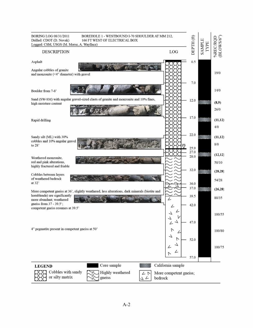
A-2
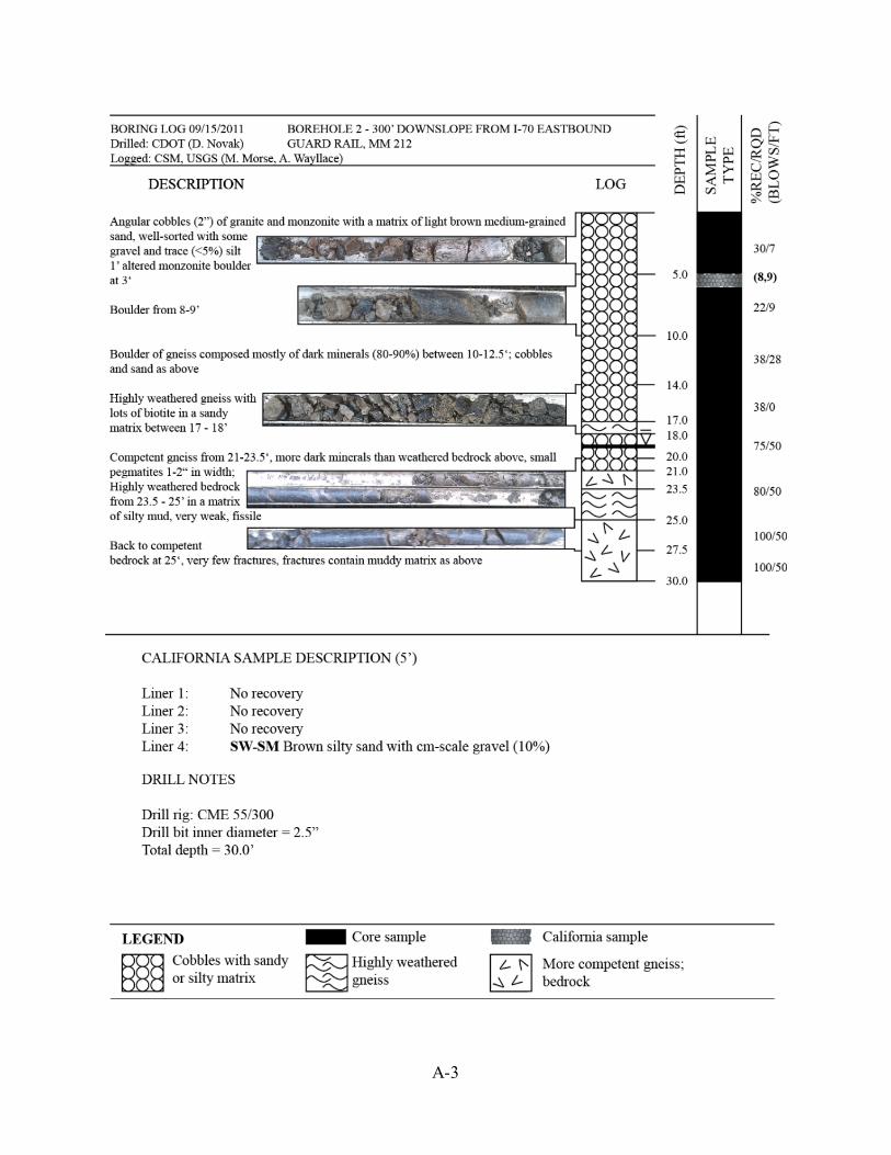
A-3
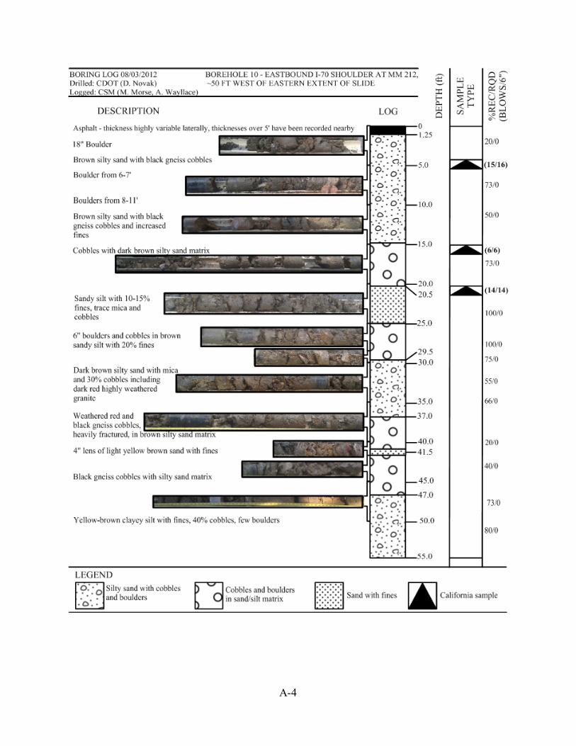
A-4
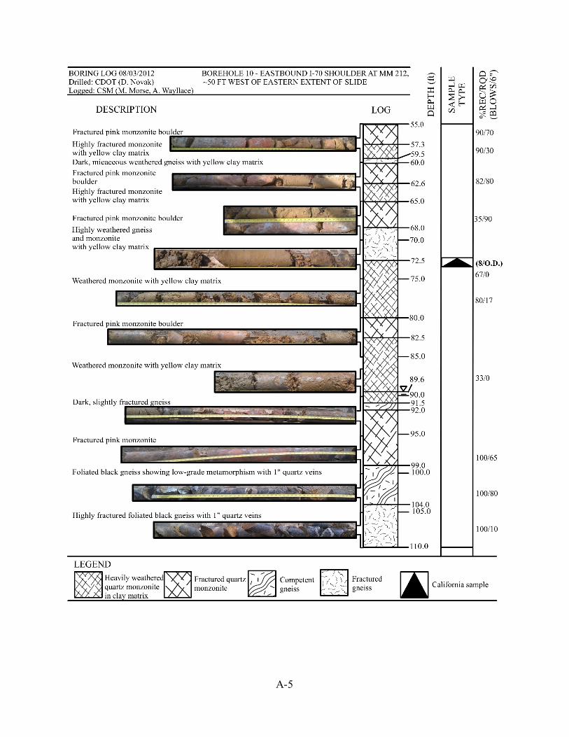
A-5
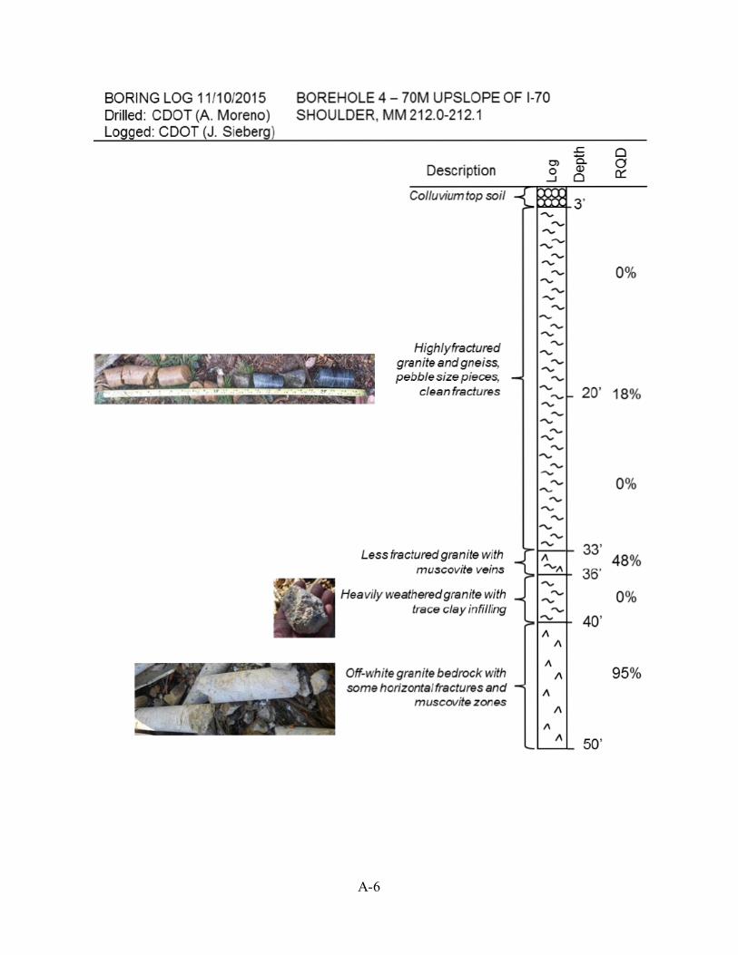
A-6
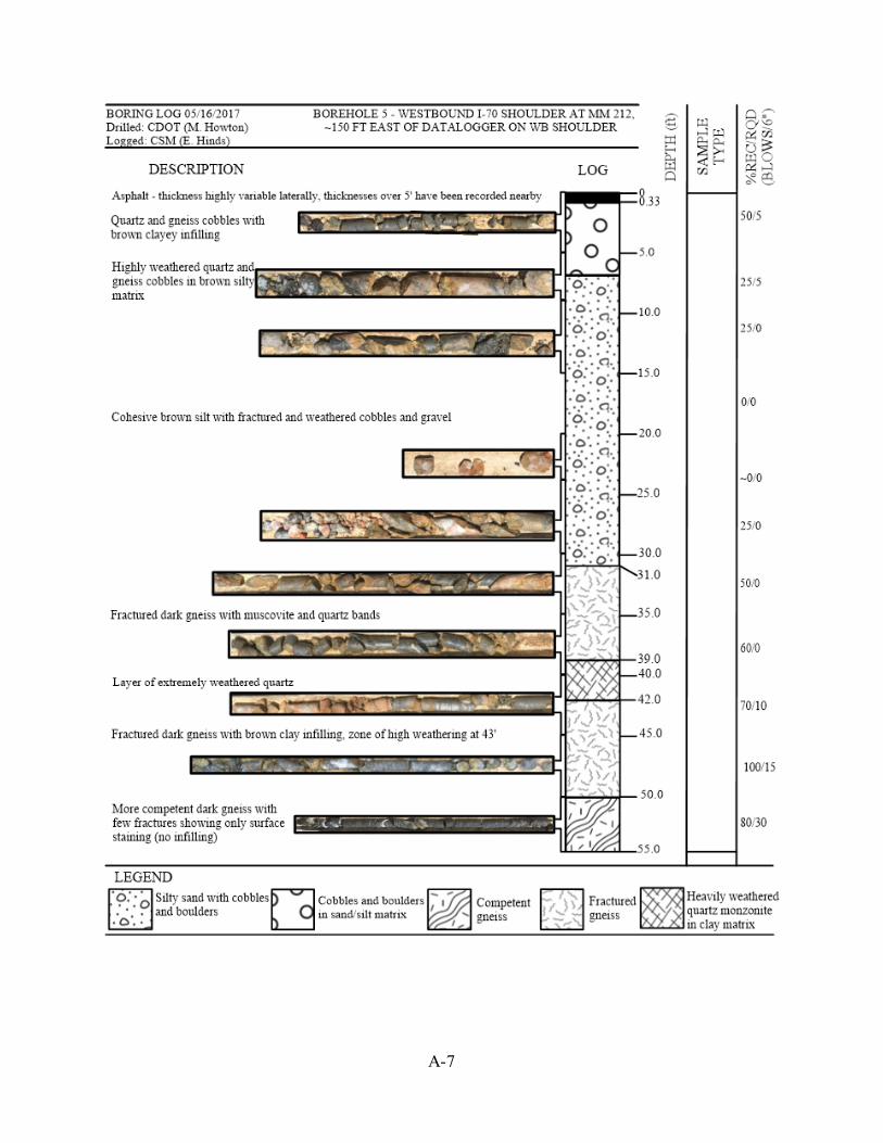
A-7
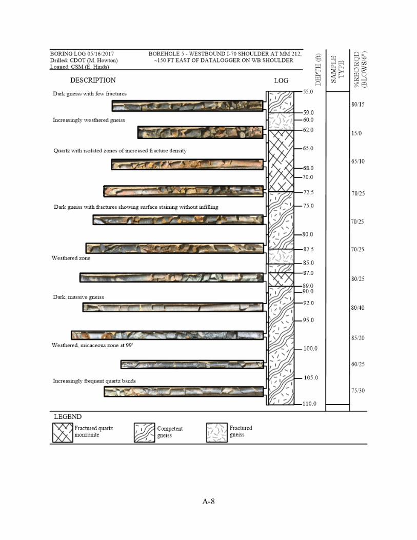
A-8

A-9
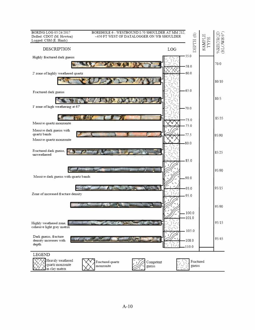
A-10
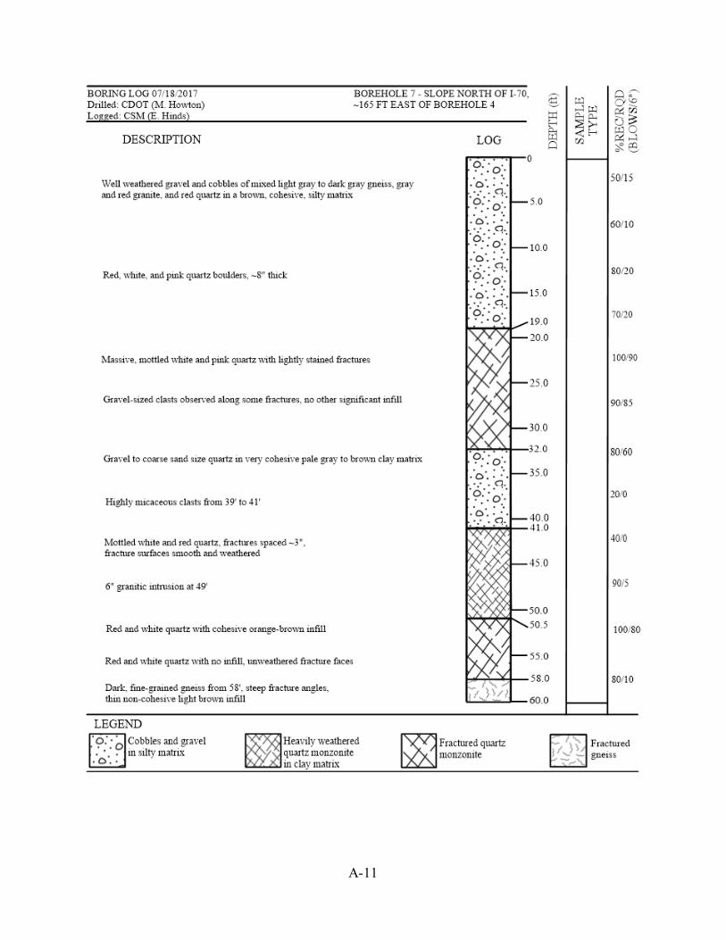
A-11
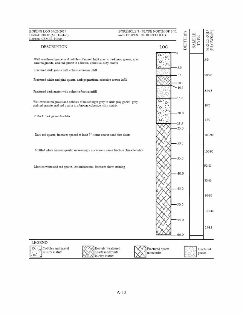
A-12

B-1
APPENDIX B FIELD INSTRUMENTATION
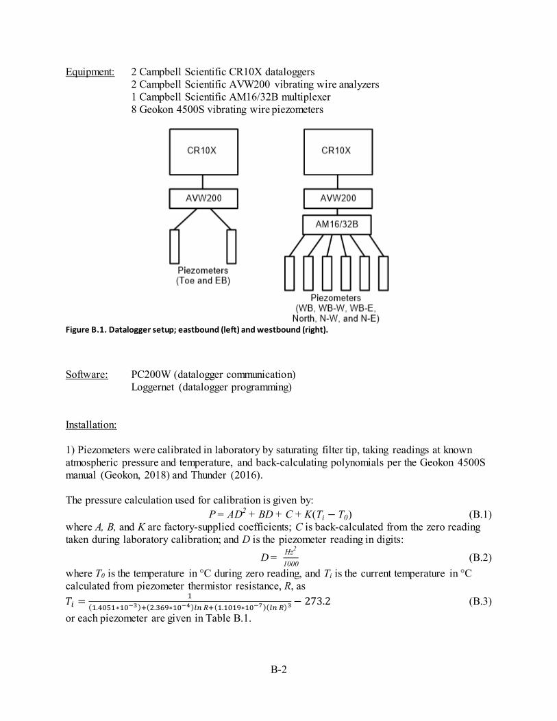
B-2
Equipment: 2 Campbell Scientific CR10X dataloggers 2 Campbell Scientific AVW200 vibrating wire analyzers 1 Campbell Scientific AM16/32B multiplexer 8 Geokon 4500S vibrating wire piezometers
Figure B.1. Datalogger setup; eastbound (left) and westbound (right).
Software: PC200W (datalogger communication) Loggernet (datalogger programming)
Installation: 1) Piezometers were calibrated in laboratory by saturating filter tip, taking readings at known atmospheric pressure and temperature, and back-calculating polynomials per the Geokon 4500S manual (Geokon, 2018) and Thunder (2016). The pressure calculation used for calibration is given by:
P = AD2 + BD + C + K(Ti − T0) (B.1) where A, B, and K are factory-supplied coefficients; C is back-calculated from the zero reading taken during laboratory calibration; and D is the piezometer reading in digits:
D = Hz2
1000 (B.2)
where T0 is the temperature in °C during zero reading, and Ti is the current temperature in °C calculated from piezometer thermistor resistance, R, as 𝑇𝑇𝑖𝑖 = 1
(1.4051∗10−3)+(2.369∗10−4)𝑙𝑙𝑙𝑙 𝑅𝑅+(1.1019∗10−7)(𝑙𝑙𝑙𝑙 𝑅𝑅)3 − 273.2 (B.3) or each piezometer are given in Table B.1.
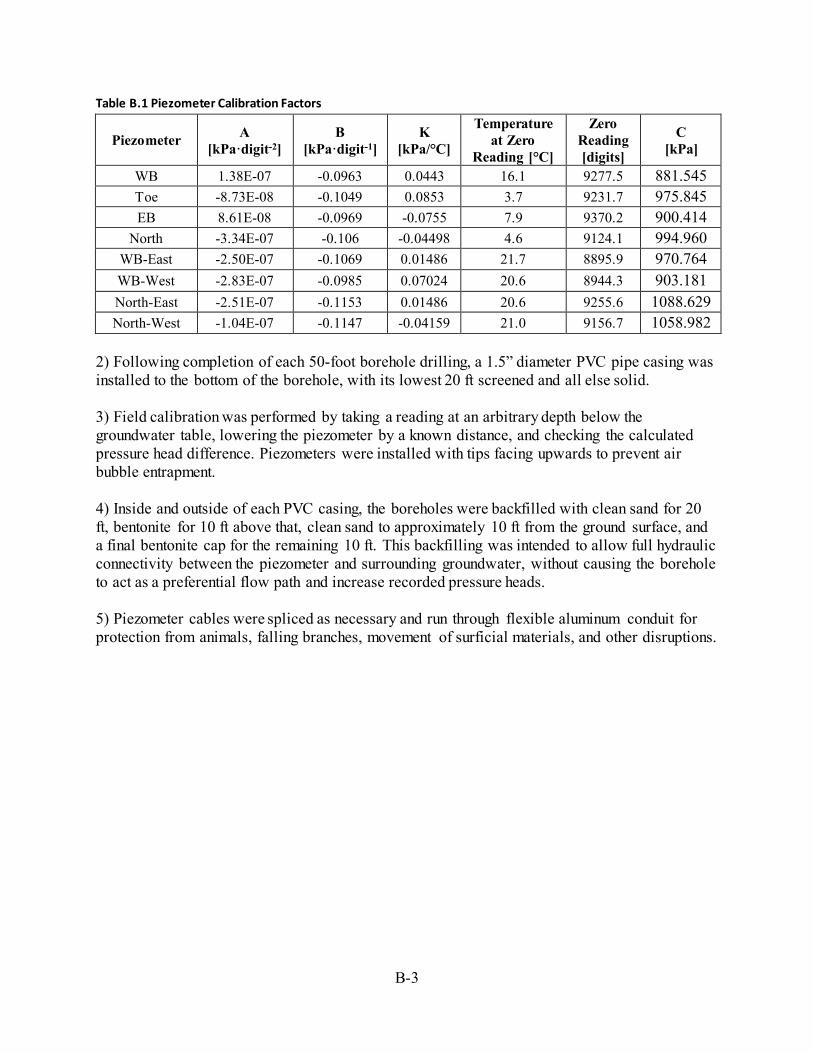
B-3
Table B.1 Piezometer Calibration Factors
Piezometer A [kPa·digit-2]
B [kPa·digit-1]
K [kPa/°C]
Temperature at Zero
Reading [°C]
Zero Reading [digits]
C [kPa]
WB 1.38E-07 -0.0963 0.0443 16.1 9277.5 881.545 Toe -8.73E-08 -0.1049 0.0853 3.7 9231.7 975.845 EB 8.61E-08 -0.0969 -0.0755 7.9 9370.2 900.414
North -3.34E-07 -0.106 -0.04498 4.6 9124.1 994.960 WB-East -2.50E-07 -0.1069 0.01486 21.7 8895.9 970.764 WB-West -2.83E-07 -0.0985 0.07024 20.6 8944.3 903.181 North-East -2.51E-07 -0.1153 0.01486 20.6 9255.6 1088.629 North-West -1.04E-07 -0.1147 -0.04159 21.0 9156.7 1058.982
2) Following completion of each 50-foot borehole drilling, a 1.5” diameter PVC pipe casing was installed to the bottom of the borehole, with its lowest 20 ft screened and all else solid. 3) Field calibration was performed by taking a reading at an arbitrary depth below the groundwater table, lowering the piezometer by a known distance, and checking the calculated pressure head difference. Piezometers were installed with tips facing upwards to prevent air bubble entrapment. 4) Inside and outside of each PVC casing, the boreholes were backfilled with clean sand for 20 ft, bentonite for 10 ft above that, clean sand to approximately 10 ft from the ground surface, and a final bentonite cap for the remaining 10 ft. This backfilling was intended to allow full hydraulic connectivity between the piezometer and surrounding groundwater, without causing the borehole to act as a preferential flow path and increase recorded pressure heads. 5) Piezometer cables were spliced as necessary and run through flexible aluminum conduit for protection from animals, falling branches, movement of surficial materials, and other disruptions.

C-1
APPENDIX C List of *.csv data files
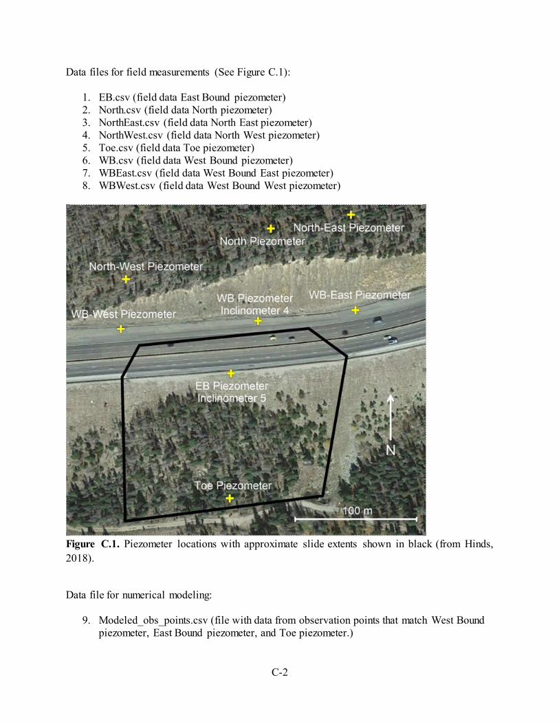
C-2
Data files for field measurements (See Figure C.1):
1. EB.csv (field data East Bound piezometer)2. North.csv (field data North piezometer)3. NorthEast.csv (field data North East piezometer)4. NorthWest.csv (field data North West piezometer)5. Toe.csv (field data Toe piezometer)6. WB.csv (field data West Bound piezometer)7. WBEast.csv (field data West Bound East piezometer)8. WBWest.csv (field data West Bound West piezometer)
Figure C.1. Piezometer locations with approximate slide extents shown in black (from Hinds, 2018).
Data file for numerical modeling:
9. Modeled_obs_points.csv (file with data from observation points that match West Boundpiezometer, East Bound piezometer, and Toe piezometer.)