Repo Market Functioning: The Role of Capital Regulation by

Antonis Kotidis and Neeltje van Horen*

October, 2018

Abstract

We exploit a novel regulatory change in the UK to identify an exogenous tightening of the leverage ratio and study its impact on the bilateral repo market. Using unique supervisory transaction-level data covering the near-universe of bilateral repo trades, we find that dealers subject to a tighter leverage ratio reduce liquidity in the market, primarily affecting their smaller clients. This finding holds when controlling for changes in demand and credit risk at the client level and concurrent factors at the dealer level. Consistent with a supply shock we further document a reduction in frequency of transactions and a worsening of repo pricing, but no adjustment in haircuts or maturities. Finally we find evidence of market resilience, based on existing, rather than new repo relationships, with foreign, non-constrained dealers stepping in.

JEL Classification Codes: F14, F15, F21, F36, G21

Keywords: Capital regulation, leverage ratio, bilateral repo market, non-bank financial institutions

                                                            

* Antonis Kotidis is a Ph.D. candidate at the University of Bonn and Neeltje van Horen is at the Bank of England and CEPR. We would like to thank Jack Bao (discussant) Ata Can Bertay, Stijn Claessens, Narly Dwarkasing (discussant), Balinth Horvath (discussant), Anil Kashyap, Daniel Paravisini, Jose-Luis Peydro, Antonio Scalia (discussant), Isabel Schnabel, Antoinette Schoar, Sjoerd Van Bekkum, Vikrant Vig, Guillaume Vuillemey (discussant), Wolf Wagner, Kathy Yuan (discussant) and conference and seminar participants at 8th BIS Research Network Meeting “Assessing the Impact of Post-Crisis Regulatory Reforms” (Basel), CEPR European Summer Symposium in Financial Markets (Gerzensee), BoE/CEPR/Imperial/LSE Conference on Non-Bank Financial Institutions and Financial Stability (London), 4th IWH-FIN-FIRE Workshop on “Challenges to Financial Stability” (Halle), the Bank of Italy/BIS Research Task Force Joint Conference on “The Impact of Regulation on Financial System and Macroeconomy”, 1st CRC 224 Conference (Offenbach), the 2nd London Financial Intermediation Workshop, the 2nd Bristol Workshop on Banking and Financial Intermediation, European Central Bank, Frankfurt School of Management, Bank of England, De Nederlandsche Bank, Copenhagen Business School, Erasmus University, University of Bonn and Lund University for helpful comments and suggestions, and Andreea Bicu, Paul Burton, Andrew Butcher, David Elliot, Gerardo Ferrara, Amy Jiang, Richard Gordon, Rob Harris, James Howat, Antoine Lallour, Ben Morley, Rishar Ramazanov, Louise Oscarius, Rupal Patel, Thomas Papavranoussis, and Jonathan Smith for sharing their insights in the UK repo market, the introduction of the leverage ratio in the UK and their help with the SMM database. The opinions expressed in this paper are those of the authros and do not necessarily reflect those of the Bank of England or its staff. E-mail addresses: s3ankoti@uni-bonn.de; Neeltje.Vanhoren@bankofengland.co.uk.

1

“In the context of evaluating the impact of post-crisis regulatory reforms, concerns have been raised that some of the measures introduced have had a negative impact on the functioning of repo markets. Market analysts and industry associations have argued

that regulatory reforms have significantly reduced the willingness of banks to provide repo services.”

Financial Stability Review, ECB, November 2017

1. Introduction

The market for repurchase agreements (repos) is a critical part of the financial system with around

12 trillion dollar of repo and reverse repo outstanding globally (CGFS, 2017).1 The market is a key

source of short-term funding for banks and other leveraged institutions. It provides a low risk

option for cash investment for banks, non-bank financial institutions and corporates and it is the

main vehicle of sourcing and financing (government) bonds. As such the repo market plays a key

role in facilitating the flow of cash and securities around the financial system and by supporting

liquidity in other markets it contributes to the efficient allocation of capital to the real economy.2 A

well-functioning repo market is thus crucial for financial stability and for the efficient transmission

of monetary policy.

However, in the wake of the financial crisis dynamics in the repo market changed

considerably. Liquidity in core repo markets dropped, costs faced by some agents increased and

repo market functioning weakened (Bank of England, 2016; Duffie, 2016; CGFS, 2017). It is

argued that Basel III regulatory reforms, most notably the leverage ratio, played an important role

in this (Duffie, 2016; CGFS, 2017). By exploiting a novel quasi-natural experiment, this paper

shows that the leverage ratio indeed affects liquidity in the bilateral repo market, however with

important heterogeneous and competition effects.

As opposed to the capital ratio, the leverage ratio is a non-risk weighted measure that

requires banks to hold capital in proportion to the overall size of their balance sheet. Due to its non-

risk weighted nature a binding leverage ratio makes it more costly to engage in low margin

activities.3 This potentially has implications for repo intermediation. The margin on repos is low

but they expand a bank’s balance sheet and therefore attract a capital charge under the leverage

ratio (Figure 1). As a result, the leverage ratio makes engaging in repo activities more costly

                                                            1 A repo is essentially a secured loan. A dealer sells a debt security, usually a government bond, to another party in exchange for cash and agrees to repurchase it for an equivalent security at a specified date. Reverse repo is the same transaction but seen from the point of view of cash lender. 2 Furthermore, since the Libor scandal several central banks have recently selected benchmark rates based on transactions in the repo market. 3 For example, assuming a Tier 1 risk-weighted asset (RWA) capital ratio requirement of 6 percent and a Tier 1 leverage ratio requirement of 3 percent, any asset on the firm’s balance sheet that is risk-weighted below 50 percent would attract higher capital requirements under the leverage ratio than under the Tier 1 RWA capital requirements.

2

relative to engaging in activities with higher margins (but equal capital charge). Banks can hence

be expected to react to this increase in costs by limiting their repo market activity.

Providing evidence of a causal impact of the leverage ratio on repo market liquidity is

challenging. While insightful, focusing on its announcement or implementation date (e.g. Bicu,

Chen and Elliott, 2017; Allahrakha, Cetina and Munyan, 2018) makes it hard to pinpoint the exact

impact of the leverage ratio due to anticipation effects. Furthermore, after the financial crisis many

countries introduced several new regulations more or less simultaneously.4 This makes it difficult

to separate the effect of the leverage ratio from the effect of other regulatory constraints, including

its impact on a bank’s desire to window-dress its balance sheet at quarter- or year-ends (Munyan,

2015, Anbil and Senyuz, 2018).5 Finally, even when confounding factors are adequately controlled

for, one has to be able to convincingly control for changes in demand and credit risk in order to

isolate a supply shock. This can only be done when detailed transaction level data are available.

To address these empirical challenges we exploit, for the first time, a change in reporting

requirements that took place in the UK, one of the world’s core repo markets. We combine this

policy shock with new very detailed supervisory transaction-level data to further tighten the

identification. From January 2016 onwards the seven largest (stress-tested) UK regulated banks

became formally subject to a 3 percent leverage ratio which they were required to report to the

regulator on a quarterly basis (Bank of England, 2015a,b).6 During a transitional period of 12

months, reporting banks could measure their on-balance sheet assets on the last day of each month

and take the average over the quarter (“monthly averaging”).7 From January 2017 onwards, the on-

balance sheet assets had to be measured on each day (“daily averaging”). Both the capital measure

as well as the off-balance sheet assets continued to be measured at month-end. This switch from

monthly to daily averaging in relation to on-balance sheet assets reduced the ability of banks to

                                                            4 For example, in the US the supplementary leverage ratio was implemented around the same time as the liquidity coverage ratio was introduced and a change in the capital treatment of investment securities came into effect, all policies that can affect repo intermediation. 5 Recently repo markets have been characterized by volatilities in prices and volumes over period ends (quarter-ends and year-ends) as banks are reducing the size or improving the composition of their balance sheets at these times. It is argued that regulatory constraints, including the leverage ratio, are one of the drivers behind window-dressing behavior of European dealers (Anbil and Senyuz, 2018). Munyan (2015) argues that unlike non-US dealers, US dealers had no incentive to engage in window-dressing as they report capital ratios based on daily averaging. 6 These are Barclays, HSBC, Nationwide, Lloyds, RBS, Santander and Standard Chartered. 7 The leverage ratio is defined as a bank’s Tier 1 capital divided by its total exposure measure which consists of the bank’s total on-balance sheet assets and certain off-balance sheet exposures.

3

window-dress their balance sheet at period-ends and effectively made the leverage ratio more

binding.8

The change in reporting requirement of the leverage ratio affected four dealers in the gilt

repo market, but not the remaining 12 dealers, providing us with a natural treatment and control

group.9 Furthermore, the change did not coincide with any other regulatory change or adjustment in

(unconventional) monetary policy in the UK potentially affecting repo markets. In addition, even

though the change in reporting was already announced in November 2015, affected banks had no

incentive to adjust their behaviour prior to the actual change in January 2017. Finally, all UK

dealers had an incentive to adjust their repo activity even when not close to the regulatory

constraint in order to avoid the market reacting to a change in their leverage ratio.

These features make it an ideal quasi-natural experiment to study if and how capital

regulation affects repo market functioning. And, as is apparent from the top panel of Figure 2, the

four dealers affected by the regulatory change indeed reacted strongly. The graph depicts the

evolution of the (standardized) total repo volume intermediated by these dealers over the period

October 2016 to February 2017. During the period of “monthly averaging” they reduced repo

volumes at each month-end, in line with window-dressing behaviour. After the move to “daily

averaging” we do not observe such behaviour anymore, indicating that the leverage ratio

effectively became more binding. As expected, the non-affected dealers did not change their

behaviour (Figure 2, bottom panel).

Exploiting this exogenous tightening of the leverage ratio, we assess how dealers adjusted

their repo intermediation in the bilateral repo market. Bilateral repo is a key segment of the repo

market (capturing around 50 and 70 percent of all repo trades in the US and UK respectively), but

due to lack of data, hitherto has not been studied in detail.10 The bilateral market differs

importantly from the US tri-party repo market which, as data are publicly available, has received

much more attention (see, e.g., Munyan, 2015, Allahrakha, Cetina and Munyan, 2018, Anbil and

                                                            8 See also ICMA European repo and collateral council report (February 2017) which argues that daily averaging reduces overall balance sheet capacity throughout the year. In other words, the shock we exploit is expected to work through the leverage ratio constraint. 9 The affected dealers are Barclays, HSBC, Lloyds and Santander. The unaffected dealers are Bank of America-Merrill Lynch, BNP Paribas, Citigroup, Deutsche Bank, Goldman Sachs, JP Morgan, Morgan Stanley, Nomura, RBC, Scotiabank, TD Bank and UBS. 10 To the best of our knowledge, the UK is the only core repo market with comprehensive data on bilateral repo. In 2014, the Office of Financial Research and the Federal Reserve System launched a voluntary pilot data collection focused on the US bilateral repo market, but comprehensive data is still lacking (Baklanova, Caglio, Cipriani and Copeland, 2016).

4

Senyuz, 2018, in the context of the impact of regulatory changes). In the US tri-party market,

institutional investors, primarily money market funds, lend cash to broker-dealers against general

collateral. The bilateral repo market is used instead by end-users (i.e. hedge funds, pension funds,

insurance companies) to either borrow cash from dealers or to invest cash low risk and obtain

(specific) securities, which in turn are used in derivative or cross-border transactions. The market

offers the possibility of re-hypothecation, the re-use of collateral in an unrelated transaction with a

third counterparty, something not possible in the US tri-party market. Dealers’ incentives to

participate in both markets and to reserve balance sheet space differ and as such inferences based

on one market cannot necessarily be extrapolated to the other one, making it critical to study both.11

As we focus on the bilateral dealer-client market we study how a tightening of the leverage

ratio affects the ability of end-users to invest cash low risk and obtain securities. This not only

compliments the literature studying the impact of regulatory changes on US tri-party repo, but it

also provides unique insights in how banking regulation spills over to non-regulated financial

institutions and corporates that interact with leverage constrained dealers. Furthermore, it provides

us with the opportunity to examine how the leverage ratio affects a more diverse set of repo market

end-users depending on their size, relationship with the dealer and sector.12 To the best of our

knowledge, this is the first paper studying the heterogeneous effects of capital regulation on repo

markets.

We employ a new supervisory database, the Sterling Money Market Database (SMMD),

which contains very detailed transaction-level data covering the near-universe of gilt repo

transactions. The database has two unique advantages. First, besides detailed information on the

volume, pricing, maturity, haircuts and collateral used in each transaction, it importantly includes

                                                            11 This argument is also made by Gorton, Laarits and Metrick (2018) in the context of the literature on the run on repo during the global financial crisis. While the impact of the financial crisis was quite subdued in the US tri-party market and the CCP intermediated European interbank market, the US and European bilateral repo markets experienced a contraction and a sharp increase in haircuts (see Gorton and Metrick, 2012, Krishnamurthy, Nagel and Orlov, 2014, Copeland, Martin and Walker, 2014 and Mancini, Ranaldo and Wrampelmeyer, 2015). This shows that it is important to critically assess all key segments of the repo market in order to fully understand its functioning. 12 Importantly the repo trades we focus on are not cleared via a Central Clearing Party (CCP). This reduces the ability of banks to net out a repo with a reverse repo transaction and as such avoid a capital charge. A bank can net out its repo with a reverse repo transaction when it involves transactions to the same counterparty, with the same maturity date and conducted in the same settlement system. This repo transaction then does not count towards the balance sheet anymore and therefore lowers the bank’s leverage ratio. Transactions via the CCP are considered transactions to the same counterparty and therefore much more likely to be eligible for netting. As such the leverage ratio is not expected to reduce liquidity in this segment of the repo market. In the UK the vast majority of interdealer trades are cleared by a CCP.

5

both the reporting dealer (the cash borrower) and the counterparty (the cash lender). This enables

us to compare adjustments in repo intermediation at the dealer-client level allowing for a much

tighter identification. Furthermore, as we know each counterparty, we are able to study whether the

leverage ratio affects different clients differently. Second, the database clearly identifies each gilt

repo transaction. As such, we do not have to rely on a matching algorithm along the lines of

Furfine (1999) in order to isolate gilt repo transactions from other transactions and to identify both

sides of the transaction.13

In a standard difference-in-differences setting, we compare repo intermediation within

dealer-client pairs before and after the policy shock differentiating between affected dealers

(treatment group) and non-affected dealers (control group). For identification purposes, we focus

on clients with at least two dealers and control for observed and unobserved heterogeneity in repo

demand and credit risk by employing client fixed effects (Kwaja and Mian, 2008). In other words,

for the same client, we compare the differential adjustment in repo volumes by affected and non-

affected dealers.

Our main results are as follows. First, we find that dealers affected by the leverage ratio on

average reduced repo volume (i.e. accepted less cash) from their clients relative to non-affected

dealers. Critically, this result holds when controlling for changes in demand and credit risk at the

client level. The economic magnitude of this change is substantial. On average, affected dealers

accept 49 percentage points less repo volumes compared to non-affected dealers from the same

client in the period after the policy change compared to the period before. 14

This effect, however, hides some important heterogeneous effects. Motivated by the CGFS

(2017) report on repo market functioning, we first differentiate between small and large clients (as

measured by their total repo activity in the period prior to the regulatory change) and find that

dealer banks subject to the regulatory change reduced repo volume more to their smaller clients

compared to their larger clients, relative to non-affected dealers. These results hold when

controlling for demand and concurrent factors potentially affecting individual dealers. We also find

that dealers tend to move away from clients with whom they have a weaker relationship; however

                                                            13 When using datasets such as Target2 and Fedwire, the use of algorithms is necessary so the output includes transactions that do not represent transactions that are of interest to the researcher or may discard transactions that should be included and these types of errors can be large (Armantier and Copeland, 2012). 14 This magnitude reflects the combined effect of affected dealers reducing repo volume they accept from their clients and the non-affected dealers increasing it.

6

the impact of size dominates. We do not find a differential effect for clients with more long-term

repos, that tend to be cash borrowers or that are foreign.

Economic effects are large with affected dealers intermediating on average 74 percentage

points lower repo volumes from their small relative to their large clients compared to non-affected

dealers.15 We show that this differential behavior is persistent, consistent with the manifestation of

a permanent change in repo market intermediation. Furthermore, affected dealers were not

behaving differently prior to the regulatory change reducing concerns that our results are driven by

different pre-event trends between the two types of dealers.

When examining the impact on the extensive margin and other loan terms, we document a

(persistent) reduction in the frequency of transactions and a reduction in repo rates that affected

dealers are willing to offer to their (small) clients. We do not find an adjustment in haircuts or

maturities. These findings are consistent with a supply shock as the tightening of the leverage ratio

should only affect volumes and prices. Bigger haircuts reflect a worsening of the quality of the

underlying collateral and maturities mainly relate to a client’s business model, so both should not

be affected by the intensification of the leverage ratio.16

The heterogeneous effects we document are in line with evidence gathered from market

participants (CGFS, 2017) and puts rigor to the causal interpretation of our findings. As

interactions with large clients are much more frequent, profit margins and franchise value tend to

be higher. In addition, larger clients more likely provide ancillary business which justifies use of

balance sheet and have more negotiating power over the contract terms. Finally, with larger clients

it is more likely that a dealer can net out a repo with a reverse repo transaction which implies that

the transaction does not count towards the balance sheet. As such, dealer banks are expected to

adjust their repo intermediation to small relative to large clients, in line with our findings.

In the final section of the paper we investigate the aggregate effect and repo substitution. A

conservative back of the envelope calculation suggests that, keeping all else equal and not allowing

for the possibility of substitution, the withdrawal of affected dealers resulted in small clients being

able to place 32 percent, equaling 2.9 billion pounds, less cash in the gilt repo market. However,

we find evidence that this is partially offset by non-affected dealers increasing their repo activity to

                                                            15 This magnitude again reflects the combined effect of affected dealers reducing the repo volume they accept from their small clients relative to their large clients, while non-affected dealers are increasing theirs. 16 Our non-result is in line with the notion that collateral and maturity are substitute mechanisms in mitigating agency problems (e.g. Ortiz-Molina and Penas, 2008).

7

these clients. This was primarily done through an intensification of pre-existing relationships,

rather than through the establishment of new ones. In line with this, non-affected dealers increased

their market share to small clients from 39 to 49 percent after the regulatory change. These results

indicate that competing, non-constrained, foreign dealers took the opportunity to capture market

share when affected, UK dealers withdrew from the small end-user segment of the dealer-client

market. The market therefore seems to have been resilient and adjusted quickly.

The remainder of the paper is structured as follows. The next section provides a review of

the literature. In Section 3 we describe in more detail the gilt repo market and how the leverage

ratio affects repo market intermediation. Section 4 outlines our empirical methodology and

describes the SMM database that we exploit. Section 5 presents and discusses our empirical

findings and Section 6 analyses the aggregate effect and market adjustment. Section 7 concludes

and discusses the policy implications of our findings.

2. Related literature

Our paper contributes to and combines two main strands of the literature. First, it contributes to the

literature that studies the repo market. Most recent studies have focused on the functioning of the

US repo market around the global financial crisis (Gorton and Metrick, 2012; Krishnamurthy,

Nagel, and Orlov, 2014 ; Copeland, Martin, and Walker, 2014) or the European repo market

around the sovereign debt crisis (Mancini, Ranaldo and Wrampelmeyer, 2016; Boissel, Derrien,

Ors and Thesmar, 2017), broadly concluding that both markets resisted the stress fairly well with

no significant decline in volumes but with some increases in haircuts.

A more nascent part of this literature focuses explicitly on how regulation affects repo

markets. Studying the US tri-party repo market Munyan (2015) and Anbil and Senyuz (2018)

provide evidence that indicates that non-US banks reduce their repo activity around financial

reporting dates to appear better capitalized.17 Allahrakha, Cettina and Munyan (2016) document a

number of changes in the US tri-party repo market after the announcement of the leverage ratio in

the US, such as a reduction in borrowing, an increase in use of more volatile collateral and a shift

                                                            17 A related literature studies window-dressing behavior in other markets. Du, Tepper and Verdelhan (2018) document covered interest rate parity violations at quarter-ends indicating that post-crisis regulation drives a wedge between supply and demand due to costly financial intermediation. Abbassi, Iyer, Peydro and Soto (2017) find that after the ECB’s announcement of its asset quality review, reviewed banks decreased their share of riskier securities and loans and the level of overall securities and credit supply.

8

towards non-bank dealers. Using a sample of European banks, Baldo, Bucalossi and Scalia (2018)

show that repo activity outside the leverage ratio reporting dates has not decreased. Focusing

primarily on the interdealer segment of the gilt repo market, Bicu, Chen and Elliott (2017) find no

statistically significant evidence of a reduction in repo liquidity after the announcement of the

leverage ratio in the UK.

Our work extends this literature in several ways. First, we explicitly focus on the dealer-

client segment of the repo market, which hitherto received very little attention due to unavailability

of data. As this is a major segment of the repo market (more than 70 percent in the UK),

understanding its functioning is essential. Second, in contrast to the above literature, the quasi-

natural experiment that we exploit in combination with detailed transaction level data allows us to

address the empirical challenges that one faces when isolating the impact of the leverage ratio from

other confounding factors and to isolate demand from supply. This enables us to make a clean

assessment of the causal impact of the leverage ratio on repo market functioning. Third, the data

allow us to examine how capital regulation affects different clients and therefore to uncover

heterogeneous effects.

Second, our paper contributes to the literature that studies the consequences of capital

regulation. Not surprisingly, given its early introduction, most of this literature has focused on the

impact of changes in the capital ratio, showing that an increase in capital requirements (or cost)

leads banks to contract lending (see among others, Berger and Udell, 1994; Aiyar, Calomiris,

Hooley, Korniyenko and Wieladek, 2014; Jimenez, Ongena, Peydro and Saurina, 2017) with

important negative real effects on firms (Gropp, Mosk, Ongena and Wix, 2018) and that it induces

credit re-allocation towards non-bank financial intermediation (Irani, Iyer, Meisenzahl and Peydro,

2018).

While the leverage ratio has received a lot of press coverage and is discussed extensively in

policy debates, the academic literature on its impact is still relatively scarce. However it is growing

rapidly. Adrian, Boyarchenko and Shachar (2017) find evidence that indicates that leverage

regulation leads to a reduction in bond liquidity. Acosta Smith, Grill and Lang (2017) and Choi,

Holcomb and Morgan (2018) show that the leverage ratio incentivizes banks to shift their portfolio

to riskier assets but does not increase overall bank risk. Furthermore, recent research shows that the

leverage ratio discourages dealers to engage in FX trading activity (Cendese, Della Corte and

Wang, 2018) reduces their willingness to clear derivatives on behalf of clients (Acosta Smith,

9

Ferrara and Rodriguez-Tous, 2018) and to participate in spread-narrowing trades (Boyarchenko,

Eisenback, Gupta, Shachar and Van Tassel, 2018). We add to this literature by showing that the

leverage ratio affects repo market functioning with dealers moving away from smaller end-users

when the leverage ratio becomes more binding.

3. Leverage ratio and repo market intermediation

This section describes the functioning of the gilt repo market in the UK and then discusses how the

leverage ratio in general and the change in the reporting requirement in particular affect the repo

market functioning.

3.1 Gilt repo market

Formally, a repo is a “repurchase agreement”: an agreement to sell securities (referred to as

collateral) at a given price to a counterparty with the commitment to repurchase the same (or

similar) security at a specified future date for a specified price. The difference between the price at

which the security is sold and repurchased reflects an annualized interest rate known as the repo

rate. From the point of view of the cash borrower the transaction is referred to as repo, while from

the point of view of the cash lender it is referred to as reverse repo. A repo transaction is

economically equivalent to a secured loan since the securities provide credit protection in the event

that the seller (i.e. the cash borrower) is unable to complete the second leg of the transaction.

Collateral haircuts and regular margin payments further protect the lender against fluctuations in

the value of the collateral. The majority of repo transactions are overnight transactions; however a

substantial share consists of maturities ranging from a couple of days to a number of months.

Repo markets play a key role in facilitating the flow of cash and securities around the

financial system. They create and support opportunities for the low-risk investment of cash, as well

as efficient management of liquidity and collateral by financial and non-financial firms. The repo

market supports the smooth functioning of derivatives markets as it provides market participants

with means to obtain high-quality collateral that can be used as margin. Movements in short-term

repo rates change the market-based financing conditions for banks and hence their conditions for

trading with firms and households. This means that repo rates are a prime channel through which

changes in the monetary policy stance are transmitted to the broader financial system and the real

10

economy. The repo market is therefore key to the short-term liquidity needs of banks and non-bank

financial institutions and a cornerstone of the transmission of monetary policy.

Although the precise structure of the repo market varies across jurisdictions, there are two

segments: the dealer-to-dealer (interdealer) and the dealer-to-client segment (dealer-client). In the

interdealer market, dealers transact to finance their market-making inventory, source short-term

funding or invest their cash and they transact on behalf of their clients. In the dealer-client segment,

end-users meet with dealers to provide collateral in return for cash (e.g. asset managers, pension

funds, hedge funds and insurance companies) or to invest in cash while receiving collateral (e.g

money market funds or corporate treasurers). Banks in addition use reverse repo to borrow gilts for

their liquid asset buffers.

Trades can be settled in three ways: bilateral, triparty and via a Central Clearing Party

(CCP). The difference between bilateral and triparty repo is that in the latter market a third party

called a clearing bank acts as an intermediary and alleviates the administrative burden between two

parties engaging in a repo. The clearing bank does not assume the credit risk of the counterparties

in the transaction. When trades are settled through a CCP the CCP acts as the clearing bank but

also assumes the credit risk by becoming the buyer to all sellers and the seller to all buyers. Only

members of the CCP can trade through the CCP. As CCP membership is expensive it is typically

limited to large banks and dealers.

In the UK the vast majority of interdealer transactions are cleared by a CCP and this

accounts for close to 30 percent of all repo transaction volume. The dealer-client segment is almost

entirely settled bilaterally and captures almost 70 percent of total transaction volume. Only a tiny

segment of the UK repo market is settled on tri-party basis (less than 5 percent). In contrast, half of

the dealer-client segment of the US repo market segment is settled bilaterally and half is settled tri-

party via a clearing bank, such as the Bank of New York Mellon and JP Morgan Chase

(Baklanova, Dalton and Tompaidis, 2017).

The vast majority of sterling-denominated repo involves the sale and repurchase of gilts

(UK government bonds) issued by the UK Debt Management Office (DMO). Around the policy

shock there were 16 dealer banks active in the market. These are Bank of America-Merrill Lynch,

Barclays, BNP Paribas, Citigroup, Deutsche Bank, Goldman Sachs, HSBC, JP Morgan, Lloyds,

Morgan Stanley, Nomura, RBC, Santander, Scotiabank, TD Bank and UBS.18 As of mid-2016,

                                                            18 There are also two non-bank dealers active, but we do not include them in the analysis.

11

there was about 900 billion USD repo and reverse repo collateralized by gilts outstanding, which

makes the UK the fourth largest repo market (after the Euro area, US and Japan) (CGFS, 2017).

3.2 Leverage ratio

In the wake of the global financial crisis the Basel Committee of Banking Supervision (BCBS)

undertook a significant program of reform to banking regulation known as Basel III. The reform

introduced new international regulatory standards for both capitalization and liquidity risk

management. One of the key regulatory reforms was the introduction of the leverage ratio. As

opposed to the capital ratio, the leverage ratio is a non-risk weighted measure that requires banks to

hold capital in proportion to the exposure measure (including both on-balance sheet exposures and

some off-balance sheet items). The requirement constrains leverage in the banking sector and thus

helps to mitigate the risk of destabilizing deleveraging processes. Furthermore, as it is independent

of risk, the leverage ratio provides a safeguard against model risk and measurement error which

affects the capital ratio.

However, because of its non-risk weighted nature the leverage ratio effectively makes it

more costly for banks to engage in low margin activities. This potentially has implications for repo

intermediation as the margin on repos is low but they expand a bank’s balance sheet and therefore

attract a capital charge under the leverage ratio (Figure 1). As a result, the leverage ratio makes it

effectively more costly for banks to assign balance sheet to repos relative to assets with higher

margins (but equal capital charge). Banks can hence be expected to react to this increase in cost by

limiting their repo activity.

The BCBS first indicated that it planned to introduce a leverage ratio in a consultation

document in 2009 and proposed a 3 percent target in 2010 (BCBS, 2009 and 2010). At this time it

also proposed a transition path to implementation whereby banks would be required to publicly

disclose their leverage ratios starting in January 2015. In 2014, the BCBS finalized the definition of

the leverage ratio and reiterated that the leverage ratio would become a Pillar 1 requirement from

2018 onwards (BCBS, 2014).

The way domestic regulators have implemented the leverage ratio varies across

jurisdictions. UK authorities have implemented the leverage ratio earlier than the Basel and EU

timelines. The seven largest UK banks (those subject to regulatory stress-tests) have been expected

to meet a 3 percent leverage ratio since January 2014 (Bank of England, 2013). End 2015 the UK

12

leverage ratio framework was announced, stipulating a 3 percent minimum requirement for the

seven banks (Barclays, HSBC, Nationwide, Lloyds, RBS, Santander and Standard Chartered)

starting in January 2016 (Bank of England, 2015a,b). Other UK regulated banks (smaller domestic

banks and foreign subsidiaries other than Santander) will become subject to a 3 percent minimum

requirement under CRD IV to be implemented after 2019. For a detailed timeline of the

implementation of the leverage ratio in the UK see Appendix Table 1. 19

4. Empirical methodology and data

4.1 Quasi-natural experiment: Change in regulatory reporting requirements

In order to examine how the leverage ratio affects repo intermediation in the bilateral dealer-client

market, we exploit a regulatory change in the UK which modified the way banks had to report their

leverage ratio. This policy change affected some dealers in the UK sterling money market but left

the other dealers unaffected and, thus, provides us with an ideal quasi-natural experiment.

As of January 2016 four dealers in the gilt repo market, Barclays, HSBC, Lloyds and

Santander, became formally subject to a 3 percent leverage ratio which has to be reported on a

quarterly basis. During a transitional period of 12 months the reporting banks could measure their

on-balance sheet assets on the last day of each month and take the average over the quarter

(“monthly averaging”). From January 2017 onwards the on-balance sheet assets had to be

measured on each day (“daily averaging”). This switch from monthly to daily average reporting

reduced the ability of banks to window-dress their balance sheet and effectively made the leverage

ratio more binding. The remaining 12 dealers did not have to report their leverage ratio to the Bank

of England and as such were not subject to the change in this requirement providing us with a

natural treatment and control group.20

Figure 2 shows that the change in reporting requirements indeed affected the behavior of

the UK regulated dealers. It depicts the evolution of the (standardized) total repo volume

                                                            19 For a further description of how UK authorities implemented the leverage ratio see Bicu, Chen and Elliott (2017) 20 These dealers are headquartered in the EU, US and Canada and therefore (also) subject to regulation in their home markets. The US implementation of the Basel III leverage ratio is the supplementary leverage ratio that requires certain banks to hold tier 1 capital equivalent to 3 percent of total exposures. US banks that are subject to the supplementary leverage ratio began disclosing and reporting their ratios in 2015, and must be in compliance by 2018. In addition, an enhanced supplementary leverage ratio (eSLR) will come into effect in 2018 and requires G-SIBs and insured depository institutions of G-SIBs to meet a 5 percent and 6 percent minimum leverage ratio, respectively. Canadian banks have to maintain a leverage ratio that meets or exceeds 3 percent at all times since January 2015. European banks have to disclose their leverage ratio since 2015 but do not have to meet a 3 percent minimum as part of their Pilar 1 capital requirements.

13

intermediated by UK regulated (top panel) and non-UK regulated (bottom panel) dealers over the

period October 2016 to February 2017. As the graph shows, prior to the regulatory change the UK

regulated dealers substantially reduced their repo volumes around month-ends, while non-UK

regulated dealers did not. After the regulatory change the volume reductions were much less

pronounced and more in line with the behavior of non-UK regulated dealers. These patterns show

that “monthly averaging” incentivized UK regulated dealers to window-dress their balance sheet,

which after the regulatory change was not beneficial anymore.

The change in regulatory reporting provides us with plausibly exogenous variation in the

intensification of the leverage ratio in order to assess its impact on repo intermediation. Using the

change in reporting requirements instead of the introduction of the leverage ratio is useful for

several reasons. First, the policy shock is much cleaner compared to the introduction of the

leverage ratio itself. The UK regulatory authorities announced the implementation of the leverage

ratio ahead of time specifically to give banks time to gradually adjust their balance sheet. Therefore

it is hard to contribute changes in the repo market to the introduction of the leverage ratio. The

change in reporting requirement that we exploit was also announced ahead of its actual

implementation (at the end of 2015), however dealers did not have an incentive to change their

behaviour ahead of the implementation date. The vast majority of repo transactions are very short-

term, so dealers do not have to adjust their repo rates or volumes until the daily average

requirement comes into effect. This makes it possible to isolate the impact of the leverage ratio on

repo intermediation from other confounding factors. Furthermore, all UK dealers had an incentive

to adjust their repo activity even without a binding leverage in order to avoid the market reacting to

a change in their leverage ratio. Finally, and crucial for our identification, the change in regulation

did not coincide with any other regulatory changes or changes in (unconventional) monetary policy

in the UK that could affect repo market intermediation. As such, the reporting change provides us

with a suitable exogenous policy shock that affects some dealers in the gilt repo market, while

leaving others unaffected.

4.2 Identification strategy

We want to assess how the leverage ratio affects the ability of end-users such as banks, insurers,

pension funds, hedge funds and asset managers, to invest their cash low risk and to have easy

access to government securities. Having identified exogenous variation in the intensification of the

14

leverage ratio allows us to perform a difference-in-differences analysis in which we compare repo

intermediation within dealer-client pair before and after the policy shock differentiating between

dealers affected and not affected by the shock.

We compare the behaviour of the two types of dealers in the month before and after the

regulatory change. To avoid any bias from increased volatility resulting from dealers’ practices to

window-dress and adjust their balance sheets at year-end, we drop the last two business weeks of

December 2016 and the first business days of January 2017 (see Figure 2). 21 We ensure that both

the pre and post periods have the same number of week days as to assure that results are not driven

by different activity on certain days of the week. As such, our pre period ranges from November 21

to December 16, 2016 and the post period ranges from January 5 to February 1, 2017 (i.e. 4

business weeks each). We use a relatively short period of time for two reasons. One, this market is

very different from the corporate loan market: it is very short term, often overnight, and clients

tend to use the market repeatedly during a short time window. Second, as the market is affected by

unconventional monetary policy and (changes in) other regulatory requirements (CGFS, 2017), the

longer the time window around the event the more likely confounding factors will affect the

estimates. However, we show that our results remain robust when we consider alternative time

windows.

We analyse the same dealer-client pair before and after the policy shock. However, it is

crucial to also control for changes in demand and risk at the client level. Therefore we focus on

clients that were placing cash in the pre-period with at least 2 different dealers and continue to

transact with them in the post period.22 This allows us to saturate the specification with client fixed

effects and to control for both observed and unobserved heterogeneity in client fundamentals

(demand, quality and risk). In other words, for the same client, we compare the differential

adjustment in repo intermediation by affected and non-affected dealers (Khwaja and Mian, 2008).

4.3 Data

We use a new regulatory database called the Sterling Money Market Database (SMMD). The aim

of this data collection is to secure and improve information available to the Bank of England on

                                                            21 At year end both types of dealers significantly reduce their repo volumes as banks reduce the size or improve the composition of their balance sheets because of regulatory constraints such as the leverage ratio, the G-SIB surcharge and the SRF levy, and because of commercial and taxation consideration (CGFS, 2017).

22 Clients with only one dealer represent <1 percent of total repo volume in our sample.

15

conditions in the sterling money market to help the Bank meet its monetary policy and financial

stability objectives. The database contains virtually all transactions, from overnight to one year,

conducted in the secured and unsecured sterling money market as reported by the 23 most active

participants in the market (this captures about 95 percent of the total market).23 The transactions

include both repos and reverse repos secured against gilts and known as gilt repo. The database

includes transactions in both the interdealer and the dealer-client repo market, but we focus

exclusively on the latter segment of the market. We have access to five months of data: October

2016 – February 2017.

The SMM database has two unique advantages. First, besides detailed information on the

volume, pricing and collateral used in each transaction, the database importantly includes both the

reporting dealer (the cash borrower) and the counterparty (the cash lender). This allows us to

effectively compare adjustments in repo intermediation within dealer-client pairs and to examine in

detail differential adjustments across client types. Second, as the database clearly identifies gilt

repo transactions, we do not have to rely on a matching algorithm along the lines of Furfine (1999)

in order to isolate the gilt repo transactions from other transactions and to identify both sides of the

transaction, a procedure that is necessary when using transaction level datasets such as Target2 and

Fedwire. As such we can say with certainty that all transactions we capture are indeed gilt repo

transactions, that we do not wrongly exclude repo transactions from any of the reporting banks and

that the party identified as the cash lender is indeed the correct counterparty.

We clean the data in a number of ways. First, while there are 23 reporting entities, only 16

of those are dealers in the repo market. As the dealers are the biggest intermediaries we capture the

vast majority of trades (>95% in terms of repo volumes). Second, we are only interested in clients

that are banks or non-bank financial institutions, such as pension funds, hedge funds and insurance

companies, and therefore we drop all repo transactions involving non-financial corporates. In

addition, we drop dealer-client transactions in which the client is another dealer (interdealer

transactions), a State, a Central Bank or a trust, because of different business models. Third, for

most transactions counterparties are reported using either their unique legal entity identifier (LEI)

or their name (for about 70 percent of the transactions the LEI is provided). However, in a few

                                                            23 The data that are available from 1 February 2016 contain a subset of ‘early adopters’, comprising roughly 80 percent of the full population. The full reporting population is contributing since 1 July 2016. This full population of reporters is chosen to cover 95 percent of the volume of activity in the sterling money market, and may be expected to change over time to remain in line with this aim. For more information on the scope of and process for reporting, see www.bankofengland.co.uk/statistics/Documents/reporters/defs/instructions_smm.pdf.

16

instances (<10 percent of total transactions), due to privacy laws, only the sector of the

counterparty is provided. As our identification relies on changes in repo intermediation at the

dealer-client level, we cannot include transactions for which the counterparty name is not available,

hence we drop these.24 We further drop transactions with variable rate, pool or multiple collateral

and tri-party repo transactions.25

As counterparty names are provided at the legal entity level, different funds of the same

asset manager are reported as different counterparties. Although a laborious task, we manually

aggregate these different legal entities into a parent company and use this as the client in our

model.26 We take this approach as credit risk, reputation and size of the parent company will

ultimately determine to what extent a dealer will adjust its repo activity. Furthermore, focusing on

the parent company avoids classifying the same legal entity as different counterparties because

different dealers use different reporting conventions.

In order to control for demand and changes in credit risk we only include clients that were

placing cash with at least two different dealers and who continue to transact with these dealers in

the post period. Our final sample therefore contains 15 dealers, 38 clients and 126 dealer-client

pairs. On average a client interacts with 3 different dealers, but the number of dealers a client

interacts with ranges from 2 to 10. Over 80 percent of the dealer-client pairs involve clients that are

non-bank financial institutions, with the largest groups being hedge funds and asset managers.

In the period preceding the change in reporting requirements 4,218 repo transactions worth

306 billion pounds took place between our group of dealers and clients. Of those 75 percent were

overnight, 13 percent had a maturity of one week and 11 percent of more than one week. On

average a dealer-client pair interacted 33 times. The affected dealers accounted for 31 percent of

total repo volume accepted.

5. Empirical results

5.1 Baseline effect

In order to examine the impact of the exogenous intensification of the leverage ratio on repo

intermediation we estimate the following model:

                                                            24 This mainly affects transactions reported from institutions based in France. 25 Transactions with these characteristics represent less than 5 percent of total transactions. 26 A similar consolidation procedure is applied by the Office of Financial Research in the U.S. Money Market Fund Monitor data.

17

∆ , (1)

where ∆ is the pre-post change in the (log of) the total repo volume accepted by

dealer i from client j, with pre={November 21-December 16} and post={January 05-February 01}.

We aggregate the daily transactions between a dealer-client pair before and after the regulatory

change because most clients do not trade every day. Also, this way we eliminate concerns of

estimation bias due to serial correlation. The variable is winsorized at the 1 and 99th percentile.

is a dummy variable equal to 1 if the dealer was subject to the UK leverage

ratio at the time of the policy change, and to 0 otherwise; is defined as the pre-

determined ratio of frequency of repo transactions between dealer i and client j to total number of

repo transactions of dealer i 27; is a vector of client fixed effects; and is the error term. The

model is estimated using OLS and, in addition, we cluster standard errors at the dealer level. We

choose this level of clustering because the coefficient of interest varies at the dealer level, as well

as to account for the fact that changes in repo volumes are likely correlated within dealer.

Appendix Table 2 shows the definition and summary statistics of all variables used throughout the

paper.

Our coefficient of interest is . A negative coefficient for would imply that—all else

equal—affected dealers intermediate lower repo volumes after the policy change, compared to non-

affected dealers. Put differently, the numerical estimate of β captures the difference in adjustment

of repo market intermediation induced by switching from the control group to the treatment group.

The cross-section specification in first differences eliminates any time-invariant (un)observed

heterogeneity at the dealer, client and dealer-client pair level as well as shocks common to all

clients and dealers. The relationship measure controls for the importance of the client in the

dealer’s portfolio before the regulatory change. In our preferred specification we also include client

fixed effects to allow us to control for (un)observed heterogeneity in changes in client demand,

quality and risk. As such, we isolate the impact of the change in the reporting requirement of the

                                                            27 We use the definition of relationship strength put forward by Petersen and Rajan (1994). For robustness, we construct an alternative measure of relationship between dealer-client pair, defined as the pre-determined ratio of volume of repo transactions between dealer-client to total volume of repo transactions of dealer (e.g. Afonso, Kovner and Schoar, 2011). Our conclusions remain unchanged when we employ the alternative measure.

18

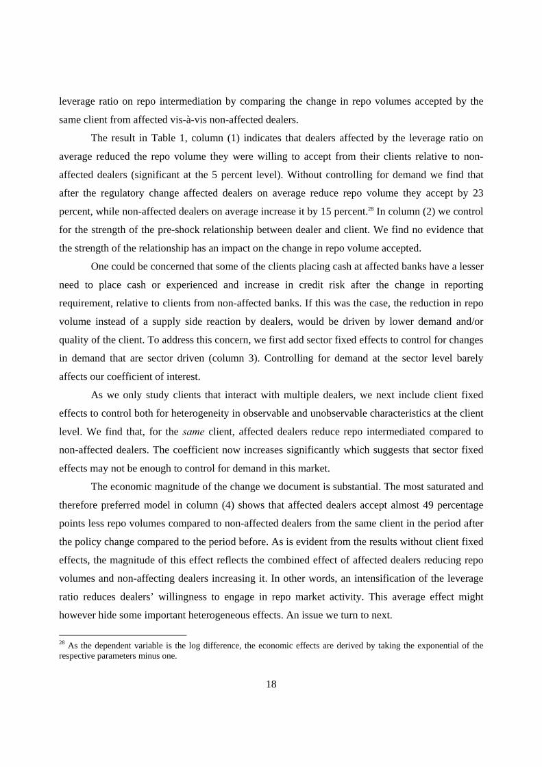
leverage ratio on repo intermediation by comparing the change in repo volumes accepted by the

same client from affected vis-à-vis non-affected dealers.

The result in Table 1, column (1) indicates that dealers affected by the leverage ratio on

average reduced the repo volume they were willing to accept from their clients relative to non-

affected dealers (significant at the 5 percent level). Without controlling for demand we find that

after the regulatory change affected dealers on average reduce repo volume they accept by 23

percent, while non-affected dealers on average increase it by 15 percent.28 In column (2) we control

for the strength of the pre-shock relationship between dealer and client. We find no evidence that

the strength of the relationship has an impact on the change in repo volume accepted.

One could be concerned that some of the clients placing cash at affected banks have a lesser

need to place cash or experienced and increase in credit risk after the change in reporting

requirement, relative to clients from non-affected banks. If this was the case, the reduction in repo

volume instead of a supply side reaction by dealers, would be driven by lower demand and/or

quality of the client. To address this concern, we first add sector fixed effects to control for changes

in demand that are sector driven (column 3). Controlling for demand at the sector level barely

affects our coefficient of interest.

As we only study clients that interact with multiple dealers, we next include client fixed

effects to control both for heterogeneity in observable and unobservable characteristics at the client

level. We find that, for the same client, affected dealers reduce repo intermediated compared to

non-affected dealers. The coefficient now increases significantly which suggests that sector fixed

effects may not be enough to control for demand in this market.

The economic magnitude of the change we document is substantial. The most saturated and

therefore preferred model in column (4) shows that affected dealers accept almost 49 percentage

points less repo volumes compared to non-affected dealers from the same client in the period after

the policy change compared to the period before. As is evident from the results without client fixed

effects, the magnitude of this effect reflects the combined effect of affected dealers reducing repo

volumes and non-affecting dealers increasing it. In other words, an intensification of the leverage

ratio reduces dealers’ willingness to engage in repo market activity. This average effect might

however hide some important heterogeneous effects. An issue we turn to next.

                                                            28 As the dependent variable is the log difference, the economic effects are derived by taking the exponential of the respective parameters minus one.

19

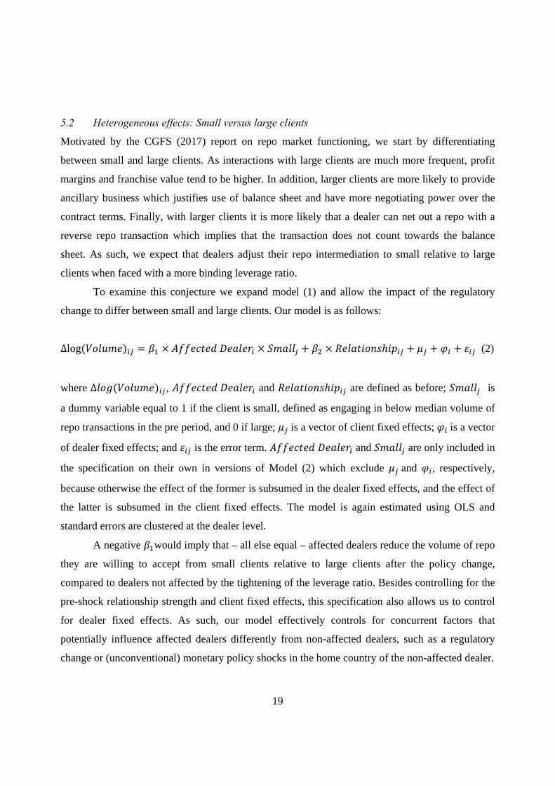
5.2 Heterogeneous effects: Small versus large clients

Motivated by the CGFS (2017) report on repo market functioning, we start by differentiating

between small and large clients. As interactions with large clients are much more frequent, profit

margins and franchise value tend to be higher. In addition, larger clients are more likely to provide

ancillary business which justifies use of balance sheet and have more negotiating power over the

contract terms. Finally, with larger clients it is more likely that a dealer can net out a repo with a

reverse repo transaction which implies that the transaction does not count towards the balance

sheet. As such, we expect that dealers adjust their repo intermediation to small relative to large

clients when faced with a more binding leverage ratio.

To examine this conjecture we expand model (1) and allow the impact of the regulatory

change to differ between small and large clients. Our model is as follows:

∆log (2)

where ∆ , and are defined as before; is

a dummy variable equal to 1 if the client is small, defined as engaging in below median volume of

repo transactions in the pre period, and 0 if large; is a vector of client fixed effects; is a vector

of dealer fixed effects; and is the error term. and are only included in

the specification on their own in versions of Model (2) which exclude and , respectively,

because otherwise the effect of the former is subsumed in the dealer fixed effects, and the effect of

the latter is subsumed in the client fixed effects. The model is again estimated using OLS and

standard errors are clustered at the dealer level.

A negative would imply that – all else equal – affected dealers reduce the volume of repo

they are willing to accept from small clients relative to large clients after the policy change,

compared to dealers not affected by the tightening of the leverage ratio. Besides controlling for the

pre-shock relationship strength and client fixed effects, this specification also allows us to control

for dealer fixed effects. As such, our model effectively controls for concurrent factors that

potentially influence affected dealers differently from non-affected dealers, such as a regulatory

change or (unconventional) monetary policy shocks in the home country of the non-affected dealer.

20

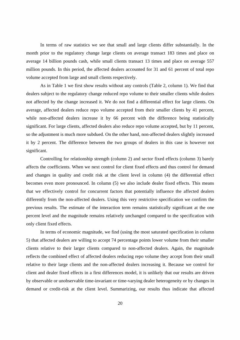
In terms of raw statistics we see that small and large clients differ substantially. In the

month prior to the regulatory change large clients on average transact 183 times and place on

average 14 billion pounds cash, while small clients transact 13 times and place on average 557

million pounds. In this period, the affected dealers accounted for 31 and 61 percent of total repo

volume accepted from large and small clients respectively.

As in Table 1 we first show results without any controls (Table 2, column 1). We find that

dealers subject to the regulatory change reduced repo volume to their smaller clients while dealers

not affected by the change increased it. We do not find a differential effect for large clients. On

average, affected dealers reduce repo volume accepted from their smaller clients by 41 percent,

while non-affected dealers increase it by 66 percent with the difference being statistically

significant. For large clients, affected dealers also reduce repo volume accepted, but by 11 percent,

so the adjustment is much more subdued. On the other hand, non-affected dealers slightly increased

it by 2 percent. The difference between the two groups of dealers in this case is however not

significant.

Controlling for relationship strength (column 2) and sector fixed effects (column 3) barely

affects the coefficients. When we next control for client fixed effects and thus control for demand

and changes in quality and credit risk at the client level in column (4) the differential effect

becomes even more pronounced. In column (5) we also include dealer fixed effects. This means

that we effectively control for concurrent factors that potentially influence the affected dealers

differently from the non-affected dealers. Using this very restrictive specification we confirm the

previous results. The estimate of the interaction term remains statistically significant at the one

percent level and the magnitude remains relatively unchanged compared to the specification with

only client fixed effects.

In terms of economic magnitude, we find (using the most saturated specification in column

5) that affected dealers are willing to accept 74 percentage points lower volume from their smaller

clients relative to their larger clients compared to non-affected dealers. Again, the magnitude

reflects the combined effect of affected dealers reducing repo volume they accept from their small

relative to their large clients and the non-affected dealers increasing it. Because we control for

client and dealer fixed effects in a first differences model, it is unlikely that our results are driven

by observable or unobservable time-invariant or time-varying dealer heterogeneity or by changes in

demand or credit-risk at the client level. Summarizing, our results thus indicate that affected

21

dealers reduced their repo market intermediation for their smaller clients as a result of the change

in reporting requirements that effectively made the leverage ratio more binding. Larger clients on

the other hand were not affected.

5.3 Heterogeneous effects: Other client types

Motivated by the CGFS (2017) report on repo market functioning, we first focused our analysis on

small vis-à-vis large clients with respect to the market as a whole. However, it is possible that

affected dealers also react differently with respect to other client characteristics. Furthermore, one

could be worried that Small dummy is a proxy for another client characteristic that might be

driving our results. Therefore in this section we examine a number of other client characteristics.

We use the same specification as in Table 2, column 5, meaning that in all regressions we control

for changes in demand and credit risk at the client level and concurrent factors at the dealer level.

First, we focus on the strength of the existing repo relationship between dealer and client

and examine how this affects the adjustment in repo intermediation. We create a dummy variable

Relationship which is one if the ratio of the frequency of repo transactions between dealer i and

client j to total number of repo transactions of the dealer in the pre-period is above the median, zero

otherwise. Since repo liquidity conditions are determined by the dealer, we want to capture the

importance of the client in the dealer’s portfolio. For this reason, we define the share within a

dealer, rather than client.

The result in Table 3, column 1 shows that a stronger relationship between dealer and client

prior to the policy change lowers the effect of the leverage ratio on repo volume and this effect is

significant at the 10 percent level. In other words, relationships seem to matter. However, when we

do a horserace between the impact of being small and having a strong relationship with the dealer,

the impact of small is dominant (column 2).29 In other words, while being an important client from

the point of view of the dealer matters, the average size of the client seems to matter more.

Next, we test whether dealers are more likely to withdraw from clients that tend to want to

place cash at longer maturities. With “daily averaging” a repo transaction with a one week maturity

would count five days towards the exposure measure, while under “monthly averaging” only one

day and only if it is on the dealers’ balance sheet at months-end. Furthermore, small clients tend on

average to have somewhat longer maturities. We create a dummy variable Long-Term Repos which

                                                            29 The correlation between the relationship and the small dummy is below 50 percent.

22

is one if the average maturity of all repo transactions of the client in the pre-period is above the

median, zero otherwise. The results in columns 3 and 4 show that the length of a normal repo

transaction does not influence an affected dealer’s decision to withdraw from a particular client.

The interaction with Small, however, remains large and statistically significant at the 5 percent

level.

Next we examine whether the adjustment is stronger for foreign clients as affected (UK)

dealers might be more willing to continue lending to domestic clients. While the parameter

estimate on the interaction with Foreign is negative, it is statistically insignificant (columns 5 and

6). Finally, we examine whether affected dealers are less likely to adjust to clients that engage

more in reverse repo. For these clients it might be easier for the dealer to net out a repo with a

reverse repo transaction and as a result the dealer might be more willing to accept repo from them.

To examine this we create a dummy variable, Reverse Repo, which is one if the client’s sector

traditionally transacts more in the reverse repo market (pension funds, insurance companies and

asset managers). The results, columns 7 and 8, show that affected dealers do not differentially

adjust to these clients. Importantly, in both cases, the interaction between affected dealer and small

remains of the same magnitude and statistically significant.

Summarizing, the defining client characteristic which determines whether a dealer faced

with an intensification of the leverage ratio adjusts its repo intermediation seems to be the size of

the client in the market. This finding is consistent with the conjecture of CGFS (2017) and market

intelligence. In the rest of the paper we therefore continue to differentiate between small and large

clients.

5.4 Dynamic effects

Up till now we focused exclusively on the period directly surrounding the change in reporting

requirements. However, it is insightful to see how the parameter on our main interaction effect

(Affected Dealer * Small) behaves over time. This allows us to examine how persistent the change

in the market is and to make sure that our results are not driven by any pre-event trends. To this

end we re-estimate our model (fully saturated with client and dealer fixed effects) but estimate the

coefficients with rolling symmetric time-windows that end or start in our original Pre period

{November 21-December 16}. The blue dots in Figure 3 indicate the estimate of and the vertical

23

lines indicate the 90 percent confidence intervals. Standard errors are again clustered at the dealer

level.

The first point estimate in the graph (labelled as Pre-1 – Pre) represents a placebo test and

examines whether in the months before the change in regulatory requirements affected and non-

affected dealers behave differently. In this regression the pre-period is moved one month back and

ranges from October 24 to November 18, 2016. The dependent variable ∆ is

defined as the log change in repo volume accepted between this period and the original pre-period

by dealer i from client j. The point estimate shows that in the months before the change in

regulatory requirements affected and non-affected dealers do not behave differently, reducing

concerns that our results are driven by different pre-event trends between the two types of dealers.30

After the change in regulatory reporting requirements, the two groups of dealers start

diverging with the parameter labelled as Pre-Post representing the point estimate of Table 2,

column 5. Importantly, the results show that this differential effect persists into February (labelled

Pre-Post+1). This finding is consistent with the manifestation of a persistent change in repo market

intermediation because of the intensification of the leverage ratio, with affected dealers moving

away from smaller clients.

5.5 Other margins of adjustment

Up till now we focused our attention on how dealers adjusted repo volumes they accepted from

their (smaller) clients. However, our database is rich and allows us to study other margins of

adjustment as well. This helps us to put rigor to the causal interpretation of our findings as one

would expect dealers to react to an intensification of the leverage ratio by adjusting volume and

prices, however it should not affect the margins that capture credit risk or business models as those

are not affected by the change in the reporting requirements.

We construct four new dependent variables. First we look at the extensive margin and

create the dependent variable Δlog(#Transactions) which is the pre-post change in the (log of) the

total number of repo transactions accepted by dealer i from client j. While our previous dependent

variable captures the outcome of the negotiation between dealer and client in terms of repo size,

                                                            30 To further mitigate such concerns, we run a second placebo experiment comparing the beginning of our data sample period (October 03 to October 21) to our Pre-1 period (October 24 to November 18). The results from this exercise again confirm that there are no pre-event trends between treatment and control group. Results are available upon request.

24

this variable captures whether the dealer and client match (i.e. the extensive margin of trading

activity). We would expect that affected dealers adjust on this margin.

In line with our expectation, we find that affected dealers after the policy change reduced

the number of transactions they engaged in with 39 percentage points compared to non-affected

dealers (Table 4, column 1). When we again allow the impact to differ across small and large

clients (column 2), we find that dealers subject to the regulatory change significantly reduced the

number of transactions they engaged in with smaller clients relative to the number of transactions

with large clients compared to dealers not affected by the change. Again, as we saturate the model

with client and dealer fixed effects this result is not driven by changes in demand or riskiness as the

client level or concurrent factors affecting dealers. In terms of economic magnitude, we find that

affected dealers reduce with 83 percentage points the number of transactions with their smaller

clients relative to larger clients compared to non-affected dealers.

Second, we study the adjustment in repo rates that affected dealers are willing to offer. If

the cost of repo increases because of the intensification of the leverage ratio, dealers can, besides

lowering the volume or the number of transactions, also lower the repo rates they are willing to

offer to clients that want to place cash. To examine whether dealers also adjust on the price

dimension we construct the dependent variable ΔRate which equals the pre-post change in the

average repo rate offered by dealer i to client j. The result in column (3) shows that following the

change in reporting requirements affected dealers were on average not adjusting repo rates to their

clients relative to non-affected dealers. However, when we allow for heterogeneous effects

(column 4) we find that affected dealers indeed adjusted repo rates offered to their small clients. In

terms of economic magnitude, we find that affected dealers are willing to pay a 9 basis points

lower repo rate to their smaller clients relative to their larger clients compared to non-affected

dealers.

Third, we examine whether dealers adjust haircuts after the change in reporting

requirements. In repo transactions haircuts are used to protect the cash lender from credit and

liquidity risk associated with the asset used as collateral. A haircut represents the difference

between the market value of the asset used as collateral in the transaction and the purchase price

paid at the start of a repo. The haircut is expressed as the percentage deduction from the market

value of collateral. As the haircut protects the cash lender against credit and liquidity risk, we

should not expect an adjustment in the wake of the intensification of the leverage ratio. Hence,

25

examining the change in haircut at the dealer-client pair level can function as a falsification test.

We construct a new dependent variable, ΔHaircut, which measures the change in the average

haircut before and after the change in reporting requirements. As expected, and in line with our

interpretation of a causal impact of the leverage ratio on repo intermediation, we do not find an

adjustment on haircuts (columns 5 and 6).

A final margin we look at is the maturity of repo. The majority of repo transactions tend to

be overnight (70 percent in our sample), however they can also have longer maturities. The

maturity requested by the end-user is often a function of their business model. For example,

insurance companies tend to opt for longer maturities compared to banks. Furthermore, the

willingness to extend longer maturity repos is also related to the riskiness of the client. For both

these reasons one would not necessarily expect a change in maturity due to the intensification of

the leverage ratio. However, on the other hand, dealers might be less willing to engage in longer

term repo after the change in regulatory reporting as now the dealer has to include the repo in its

exposure measure on each day until maturity, while before it only had to include it if it had not

matured at month-end. Our fourth dependent variable Δlog(Maturity) is defined as the pre-post

change in the (log of) the average maturity (in number of days) of the transactions between dealer i

from client j. In line with the interpretation that repo maturities reflect the business model of the

client, we do not find a change in maturities after the change in regulatory reporting. Not in general

and not for smaller clients in particular (columns 7 and 8).

Finally, we examine the dynamic adjustment for the two margins (number of transactions

and repo rates) that are adjusted by the affected dealers differentiating between small and large

clients. As with the adjustment in the repo volume, we find that in the months before the change in

regulatory requirements affected and non-affected dealers do not behave differently (Figure 4). The

two groups of dealers only start diverging after the shock and this differential effect persists.

5.6 Further robustness

In this section we set out to put further robustness to our results. We first perform an additional

falsification test by examining whether affected dealers were also reducing the volume of cash they

were willing to lend (reverse repo) after the change in regulatory requirements. Reverse repo does

not affect the balance sheet so we do not expect an impact of the intensification of the leverage

ratio. Indeed, the results in Table 5 show that affected dealers were not reducing the amount of

26

cash they were lending to their clients relative to non-affected dealers (column 1). We also do not

detect any differential effect with respect to their small clients (column 2). These results again

indicate that a reduction in repo intermediation by affected dealers can be attributed to the

intensification of the leverage ratio. 31

Next we examine the sensitivity of our results to our definition of small clients. Up till now

we identified a client as small if it engaged in below median volume of repo transactions in the pre

period. In Table 6 we first define small as a client with the number of transactions below the

median (column 1). In addition, we use three continuous variables: the log volume of the client in

the repo market (column 2), the log number of transactions of the client in the repo market (column

3) and the log volume divided by the number of transactions of the client in the repo market

(column 4), all three measured before the regulatory change. In all cases the interaction of affected

with small is of the right sign and significantly different from zero, indicating that our results are

not sensitive to our definition of small clients.

Any choice of sample period is arbitrary as it is not obvious how much time it would take

for the adjustment in the market to take place. Focusing on a short time horizon could bias the

results against finding anything because especially smaller clients might not be active in both

periods. Taking a longer time horizon increases the risk of other factors (both in the UK and

abroad) affecting the market convoluting our identification strategy. Furthermore, it is not entirely

clear how much time one should account to nullify the impact of the end-of-year volatility. To this

end we adjust in Table 7 the time period along several dimensions. In columns 1 and 2 we only

exclude the last day of the year. In columns 3 and 4 we drop the days in November as at two points

during this month there is a drop in repo volume accepted by the affected dealers. In columns 5 and

6 we expand the pre-period and have it start on October 31, 2016 and in columns 7 and 8 we

extend the post-period and have it end on February 22. Regardless of the time period we exploit,

                                                            31 It would also be insightful to examine whether the reduction in volume is stronger for repos conducted against general compared to repos conducted against special collateral. Special collateral is a repo in which the cash provider requests a specific security (individual ISIN) to be provided by the cash borrower (security-driven repos). General collateral is a repo in which the security lender may choose the security to pledge as collateral with the cash provider (cash-driven repos). When negotiating special repos, a dealer agrees on the collateral first and then the size, price and term of such transactions. As such, the rate of special repos is usually below the rate of general repos, in other words, the margin on these repos is higher. As such one would expect affected dealers to especially reduce general collateral repo. Unfortunately, our data do not allow us to identify with certainty whether repos are conducted against general or special collateral, because this field is optional to report. In our sample period, approximately 43 percent of transactions provide no such information, 24 percent are special and 33 percent are general repos.

27

our results indicate that dealer banks subject to the regulatory change reduced repo volume to their

smaller clients compared to dealer banks not affected by the change.

Finally we test whether our results are robust to different specifications and assumptions

regarding the clustering of the error terms and how we deal with outliers. In Table 8, in order to

mitigate concerns that differences in maturity drives the impact of repo volumes on dealer balance

sheets, we first re-estimate our baseline and heterogeneous models employing Weighted Least

Squares (WLS) using as weights the average maturity of transactions of dealer-client pairs before

the policy change.32 Columns 1 and 2 confirm our conclusions, although the estimate of the

interaction effect is somewhat smaller. Next, although Bertrand, Duflo and Mullainathan (2004)

show that cluster-robust standard errors still perform reasonably well with 15 clusters, we eliminate

remaining concerns by employing a wild cluster bootstrap method as recommended by Cameron,

Gelbach and Miller (2008) and Cameron and Miller (2015). This procedure allows us to account

for the correlation in the error terms of clients placing cash with the same dealer bank with

relatively few clusters. In columns 3 and 4, we report wild cluster bootstrap p-values, which

confirm our conclusions suggesting that the clustering strategy has little effect on our results.33

Finally, we employ an alternative winsorising technique at the 5th and 95th level instead of the 1st

and 99th and we find again very similar results as in our baseline models.

6. Aggregate effect and market adjustment

Finally, we investigate the aggregate effect of the intensification of the leverage ratio which

incentivised affected dealers to move away from small end-users. We can do a conservative back

of the envelope calculation and assess to what extent small end-users were affected in aggregate.

Using the OLS estimates of Table 2, column 1 we estimate that affected banks on average reduced

repo volume to their small clients with 53 percent.34 As affected dealers were prior to the

regulatory change intermediating 61 percent of total repo volume from small end-users, this

implies that, keeping all else equal and not allowing for the possibility of substitution, the

                                                            32 We also test whether our results are driven by clients trading in very long maturities. We confirm that our conclusions remain unchanged when we restrict our sample to dealer-client pairs that only engage in repo with a maturity of up to 4 weeks. 33 We generate these p-values by employing the post-estimation command boottest (Roodman, 2015), assuming the null hypothesis and setting replications to 1000. 34 This is the combined effect of the constant, the affected dummy, the small dummy and the affected*small interaction effect.

28

withdrawal of affected dealers resulted in small end-users being able to place 32 percent, equaling

2.9 billion pounds, less cash in the gilt repo market.

The next question is whether these small end-users were able to switch to other, non-

affected dealers and place their cash with them instead. To check whether indeed this was the case,

we run a set of client-level regressions with the growth rate of the client’s total repo volume as the

dependent variable. We are interested to see if small clients that were more exposed to the affected

dealers were experiencing lower growth rates compared to small clients less exposed. To this end

we construct a measure of the average exposure to affected dealers for each client before the policy

shock. That is, for each client we measure the ratio of each client's repo volumes with affected

dealers to the client's total repo volumes before the regulatory change. As we are interested in the

growth rate at the client level, we cannot absorb client demand directly with client fixed effects. If

the exposure measure is correlated with demand, something we cannot rule out, our OLS estimates

would be biased. In order to control for clients’ repo demand we follow Abowd, Kramarz and

Margolis (1999), Bonaccorsi di Patti and Sette (2016) and Cingano, Manaresi and Sette (2016) and

include in our model a vector of client-level estimated dummies that we extract from model (2)

in Section 5.2.35 The model we estimate is as follows:

∆

, (3)

where ∆ is the pre-post change in the (log of) the total repo volume accepted

by all (new and existing) dealers from client j, winsorized at the 1 and 99 percentiles.

is a dummy variable equal to 1 if the client has above median share of its repos

intermediated by affected dealers, zero otherwise; is a dummy variable equal to 1 if the

client is small, defined as engaging in below median volume of repo transactions in the pre period,

and 0 if large; is a vector of client-level estimated dummies capturing demand; and is the

error term. To account for correlation in the error terms of clients within the same sector, and given

                                                            35 Bonaccorsi di Patti and Sette (2016) and Cingano, Manaresi and Sette (2016) show that this methodology is equivalent to an alternative methodology to control for demand developed by Jimenez, Mian, Peydro and Saurina (2014), where a numerical correction of the difference of the OLS and FE estimate is applied.

29

that the number of sectors is 7, we employ the wild cluster bootstrap method of Cameron, Gelbach

and Miller (2008) and report the respective p-values.36

The result in Table 9, column 1 shows that highly exposed clients experience a lower

growth in total repo volume (i.e. the amount of cash they are placing with all dealers), but this

effect is not significant. When we allow this effect to differ between large and small clients

(column 2) we find that it is driven by the small clients, in line with our previous results. The

parameters are smaller (less negative) compared to the estimates at the dealer-client level. This

suggests that partial substitution was possible, in line with our previous finding that non-affected

dealers were on average accepting more repo from their small clients after the policy change.

In the last two columns of Table 10 we examine whether this substitution was primarily

done through an intensification of pre-existing relationships or through the establishment of new

ones. We construct a new dependent variable, New Repo Relationship, which is a dummy variable

equal to one if the client started in the month after the regulatory change a relationship with a

dealer with whom it had no relationship in the pre-period, zero otherwise. We do not find any

indication that more exposed clients are more likely to start a new relationship, which suggests that

exposed clients substitute with non-affected dealers with whom they already had a relationship and

did not switch to new dealers.

Our finding that the small end-users, particularly the ones less exposed to affected dealers,

were able to substitute with non-affected, foreign dealers is confirmed when we look at the change

in market share of affected and non-affected dealers after the intensification of the leverage ratio.

While the group of affected dealers increased their market share of the large clients from 31 to 34

percent, they reduced it from 61 to 51 percent for the smaller clients.

7. Conclusion and policy implications

This paper investigates the impact of the leverage ratio on dealer-client repo intermediation,

focusing on both bank and non-bank end-users. We exploit a new, unique, supervisory transaction-

level dataset capturing the near-universe of bilateral gilt repo market trading in combination with a

regulatory change in the UK. Studying adjustments within dealer-client pairs, we find that dealers

subject to a tightening of the leverage ratio due to a change in its reporting requirements                                                             36 Clustering at the sector level would not perform well and would lead to high rejection rates when the number of clusters is approximately 6, as suggested by Bertrand, Duflo and Mullainathan (2004).

30

persistently reduced repo volume they accepted from their small clients compared to dealers not

affected by the change. Large clients were not affected. We also find that dealers tend to move

away from clients with whom they have a weaker relationship; however the impact of size

dominates. In addition, we document a (persistent) reduction in the frequency of transactions and in

repo rates offered, but no adjustment in haircuts or maturities. Studying the aggregate effect, we

find evidence that suggests that competing, non-constrained, foreign dealers took the opportunity to

capture market share when affected, UK dealers withdrew from the small end-user segment of the

dealer-client market. The market therefore seems to have been resilient and adjusted quickly.

All in all, our results show that dealers react to an intensification of the leverage ratio by

stepping away from smaller end-users. This finding has important policy implications as it shows

that capital regulation has the potential to undermine the level playing field of small banks and

non-bank financial institutions relative to their larger competitors as the increased cost of engaging

in repo activity is disproportionately levied onto them. Without other dealers stepping in, this

implies that these smaller end-users ultimately have to pass on these costs to their clients.

Furthermore, it can incentivize them to invest their cash in more risky ways (e.g. longer maturities

or against lower quality or no collateral), it can impair their access to derivatives markets and it can

increase the cost they face when hedging interest rate risk. These effects can be mitigated if other

dealers step into the void as seems to have happened in the UK. While this can alleviate the short-

run impact of a more binding leverage ratio it has the potential to make the market more unstable.

A stronger reliance on foreign dealers can potentially imply more instability as during times of

stress foreign lenders tend to flight home (Gianetti and Laeven, 2012) and reduce lending

especially to marginal borrowers (De Haas and Van Horen, 2013).

A possible way to reduce the impact of the leverage ratio on repo market liquidity for small

end-users would be to widen participation in CCPs to end-users of repos. If end-users are members

of the same CCP as their intermediating dealer, then the dealer will be able to net the transaction

for the purpose of the regulation. In recent years there have been several initiatives, including by

the Bank of England, to reduce barriers for smaller firms to joining the CCP. Furthermore,

intermediation might be improved through competition effects by disintermediation of banks in

return for a larger role for non-bank intermediaries not subject to the leverage ratio. However, a

growing role of non-bank dealers in the repo market can also make the market more susceptible to

financial instability risks as these dealers are not regulated.

31

Importantly, our paper does not attempt to quantify the net benefits of the regulatory

leverage ratio. The leverage ratio has important benefits for the financial system as a whole. By

increasing the capitalization of banks, the leverage ratio mitigates the risk of destabilizing

deleveraging processes. Furthermore, as it is independent of risk, it provides a safeguard against

model risk and measurement error which affects the capital ratio. In addition, as there are risks

associated with excessive liquidity a lower level of liquidity in the repo market might not be sub-

optimal. While quantifying the net costs/benefits of the leverage ratio is beyond the scope of this

paper, our results indicate that the leverage ratio affects some end-users in the repo market more

than others. As such, policy measures that improve repo market liquidity for these end-users might

be useful.

32

References

Abbassi, Puriya, Rajkamal Iyer, Jose-Luis Peydro and Paul E. Soto, 2017, “Dressing up for the regulators: evidence from the largest-ever supervisory review, mimeo.

Abowd, John, Francis Kramarz and David Margolis, 1999, “High wage workers and high wage firms,” Econometrica, 67(2), 251–333.

Acosta Smith, Jonathan, Michael Grill and Jan Hannes Lang, 2017, “The leverage ratio, risk-taking and bank stability,” ECB Working Paper No. 2079.

Acosta Smith, Jonathan, Gerardo Ferrara and Francesc Rodriguez-Tous, 2018, “The impact of the leverage ratio on client clearing,” Bank of England Staff Working Paper No. 735.

Adrian, Tobias, Nina Boyarchenko and Or Shachar, 2017, “Dealer balance sheets and bond liquidity provision,” Journal of Monetary Economics, 89, 92-109.

Afonso, Gara, Anna Kovner and Antoinette Schoar, 2011, “Relationships matter: The importance of relationships in the Fed funds market,” Mimeo.

Aiyar, Shekhar, Charles W. Calomiris, John Hooley, Yevgeniya Korniyenko and Tomasz Wieladek, 2014, “The international transmission of bank capital requirements: Evidence from the UK,” Journal of Financial Economics, 113(3), 368-382.

Allahrakha, M., J. Cetina and B. Munyan, 2018, “Do higher capital standards always reduce bank risk? The impact of the Basel leverage ratio on the US tri-party repo market,” Journal of Financial Intermediation, 34, 3-16.

Anbil, Sriya and Zeynep Senyuz, 2018, “Window-dressing and the Fed’s RRP Facility in the repo market,” Finance and Economics Discussion Paper Series No. 2018-027.

Armantier, Olivier and Adam Copeland, 2012, “Assessing the quality of “Furfine-based” algorithms,” Federal Reserve Bank of New York Staff Reports No. 575.

Baldo, Luca, Annalisa Bucalossi and Antonio Scalia, 2018, “Leverage ratio and central bank operations in the Euro Area,” Economic Notes by Banca Monte dei Paschi di Siena SpA, 47, 21-68

Baklanova, Viktoria, Cecilia Caglio, Marco Cipriani and Adam Copeland, 2016, “The U.S. bilateral repo market: Lessons from a new survey,” OFR Brief Series No. 16-01

Baklanova, Viktoria, Ocean Dalton, and Stathis Tompaidis, 2017, “Benefits and risks of central clearing in the repo market,” OFR Brief Series No. 17-04

Bank of England, 2013a, “Capital and leverage ratios for major UK banks and building societies – Supervisory Statement,” November.

33

_____, 2015a, “PS27/15: Implementing a UK leverage ratio framework,” Policy Statement.

_____, 2015b, “CP24/15: Implementing a UK leverage ratio framework,” Consultation Paper.

_____, 2016, “The money market liaison committee sterling money market survey,” Survey results 2016 H1.

Berger, Allen and Gregory Udell, 1994, “Did risk-based capital allocate bank credit and cause a “credit crunch” in the United States?” Journal of Money, Credit and Banking, 26, 585-628

Bertrand, Marianne, Esther Duflo and Sendhil Mullainathan, 2004, “How much should we trust differences-in-differences estimates?” Quarterly Journal of Economics, 119, 249–275.

Bicu, Andreea, Louisa Chen and David Elliott, 2017, “The leverage ratio and liquidity in the gilt and repo markets,” Bank of England Staff Working Paper No. 690.

Boissel, Charles, Francois Derrien, Evren Ors and David Thesmar, 2017, “Systemic risk in clearing houses: Evidence from European repo market” Journal of Financial Economics, 125(3), 511–536.

Bonaccorsi di Patti and Enrico Sette, 2016, Did the securitization market freeze affect bank lending during the financial crisis? Evidence from a credit register,” Journal of Financial Intermediation, 25, 54-76.

Boyarchenko, Nina, Thomas Eisenback, Pooja Gupta, Or Shachar and Peter Van Tassel, Bank-intermediated arbitrage, Federal Reserve Bank of New York Staff Report No. 858.

BCBS, 2009, “Strengthening the resilience of the banking sector,” Consultative Document, Bank for International Settlements.

_____, 2010, “The group of governors and heads of supervision reach broad agreement on Basel committee capital and liquidity reform package,” Press Release.

_____, 2014, “Basel III leverage ratio framework and disclosure requirements.”

Cingano, Federico, Francesco Manaresi and Enrico Sette, 2016, “Does credit crunch investment down? New evidence on the real effects of the bank-lending channel,” Review of Financial Studies, 29(10), 2737-2773.

Cameron, Colin, Jonah Gelbach and Douglas Miller, 2008, “Bootstrap-based improvements for inference with clustered errors,” Review of Economics and Statistics, 90(3), 414-427.

Cameron, Colin and Douglas Miller, 2015, “A practitioner’s guide to cluster-robust inference,” Journal of Human Resources, 50(2), 317-372.

CGFS, 2017, “Repo market functioning,” CGFS Papers 59, Bank for International Settlements.

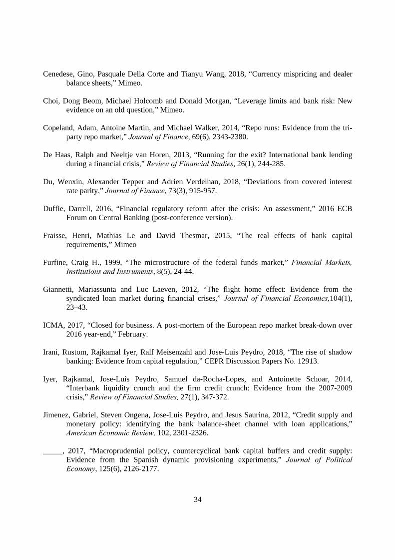
34

Cenedese, Gino, Pasquale Della Corte and Tianyu Wang, 2018, “Currency mispricing and dealer balance sheets,” Mimeo.

Choi, Dong Beom, Michael Holcomb and Donald Morgan, “Leverage limits and bank risk: New evidence on an old question,” Mimeo.

Copeland, Adam, Antoine Martin, and Michael Walker, 2014, “Repo runs: Evidence from the tri-party repo market,” Journal of Finance, 69(6), 2343-2380.

De Haas, Ralph and Neeltje van Horen, 2013, “Running for the exit? International bank lending during a financial crisis,” Review of Financial Studies, 26(1), 244-285.

Du, Wenxin, Alexander Tepper and Adrien Verdelhan, 2018, “Deviations from covered interest rate parity,” Journal of Finance, 73(3), 915-957.

Duffie, Darrell, 2016, “Financial regulatory reform after the crisis: An assessment,” 2016 ECB Forum on Central Banking (post-conference version).

Fraisse, Henri, Mathias Le and David Thesmar, 2015, “The real effects of bank capital requirements,” Mimeo

Furfine, Craig H., 1999, “The microstructure of the federal funds market,” Financial Markets, Institutions and Instruments, 8(5), 24-44.

Giannetti, Mariassunta and Luc Laeven, 2012, “The flight home effect: Evidence from the syndicated loan market during financial crises,” Journal of Financial Economics,104(1), 23–43.

ICMA, 2017, “Closed for business. A post-mortem of the European repo market break-down over 2016 year-end,” February.

Irani, Rustom, Rajkamal Iyer, Ralf Meisenzahl and Jose-Luis Peydro, 2018, “The rise of shadow banking: Evidence from capital regulation,” CEPR Discussion Papers No. 12913.

Iyer, Rajkamal, Jose-Luis Peydro, Samuel da-Rocha-Lopes, and Antoinette Schoar, 2014, “Interbank liquidity crunch and the firm credit crunch: Evidence from the 2007-2009 crisis,” Review of Financial Studies, 27(1), 347-372.

Jimenez, Gabriel, Steven Ongena, Jose-Luis Peydro, and Jesus Saurina, 2012, “Credit supply and monetary policy: identifying the bank balance-sheet channel with loan applications,” American Economic Review, 102, 2301-2326.

_____, 2017, “Macroprudential policy, countercyclical bank capital buffers and credit supply: Evidence from the Spanish dynamic provisioning experiments,” Journal of Political Economy, 125(6), 2126-2177.

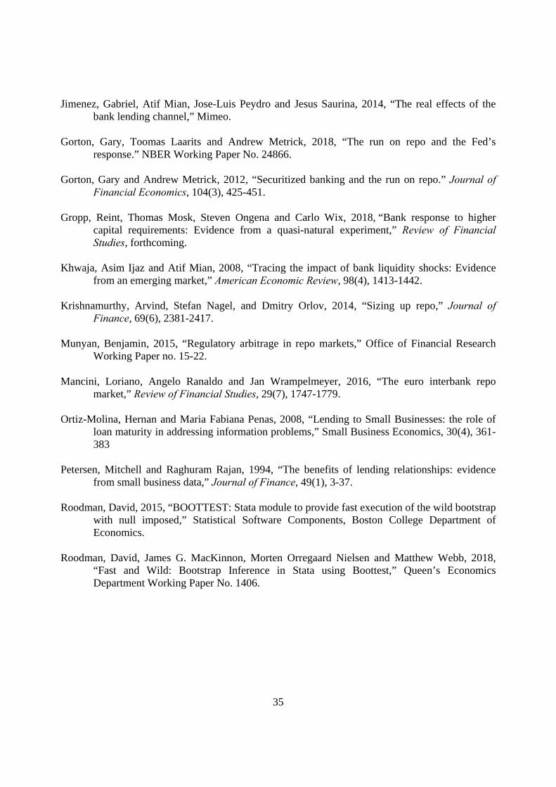
35

Jimenez, Gabriel, Atif Mian, Jose-Luis Peydro and Jesus Saurina, 2014, “The real effects of the bank lending channel,” Mimeo.

Gorton, Gary, Toomas Laarits and Andrew Metrick, 2018, “The run on repo and the Fed’s response.” NBER Working Paper No. 24866.

Gorton, Gary and Andrew Metrick, 2012, “Securitized banking and the run on repo.” Journal of Financial Economics, 104(3), 425-451.

Gropp, Reint, Thomas Mosk, Steven Ongena and Carlo Wix, 2018, “Bank response to higher capital requirements: Evidence from a quasi-natural experiment,” Review of Financial Studies, forthcoming.

Khwaja, Asim Ijaz and Atif Mian, 2008, “Tracing the impact of bank liquidity shocks: Evidence from an emerging market,” American Economic Review, 98(4), 1413-1442.

Krishnamurthy, Arvind, Stefan Nagel, and Dmitry Orlov, 2014, “Sizing up repo,” Journal of Finance, 69(6), 2381-2417.

Munyan, Benjamin, 2015, “Regulatory arbitrage in repo markets,” Office of Financial Research Working Paper no. 15-22.

Mancini, Loriano, Angelo Ranaldo and Jan Wrampelmeyer, 2016, “The euro interbank repo market,” Review of Financial Studies, 29(7), 1747-1779.

Ortiz-Molina, Hernan and Maria Fabiana Penas, 2008, “Lending to Small Businesses: the role of loan maturity in addressing information problems,” Small Business Economics, 30(4), 361-383

Petersen, Mitchell and Raghuram Rajan, 1994, “The benefits of lending relationships: evidence from small business data,” Journal of Finance, 49(1), 3-37.

Roodman, David, 2015, “BOOTTEST: Stata module to provide fast execution of the wild bootstrap with null imposed,” Statistical Software Components, Boston College Department of Economics.

Roodman, David, James G. MacKinnon, Morten Orregaard Nielsen and Matthew Webb, 2018, “Fast and Wild: Bootstrap Inference in Stata using Boottest,” Queen’s Economics Department Working Paper No. 1406.

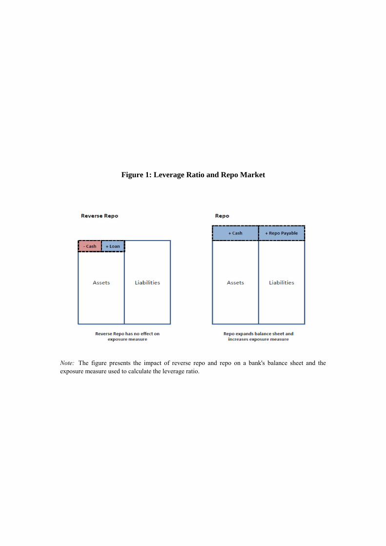
Figure 1: Leverage Ratio and Repo Market

Note: The figure presents the impact of reverse repo and repo on a bank's balance sheet and theexposure measure used to calculate the leverage ratio.

Figure 2a: Daily Repo Volume by Affected Dealers

Note: The figure presents the evolution of (standardized) repo volume intermediated by affected dealers over the periodOctober 2016 - February 2017. The vertical dashed lines correspond to month-ends before (red) and after (green) theregulatory change in the reporting requirement of the leverage ratio. The black vertical dashed lines correspond to theadjustment period before and after year-end, which we exclude from our main analysis.

Figure 2b: Daily Repo Volume by Non-Affected Dealers

Note: The figure presents the evolution of (standardized) repo volume intermediated by non-affected dealers over theperiod October 2016 - February 2017. The vertical dashed lines correspond to month-ends before (red) and after (green)the regulatory change in the reporting requirement of the leverage ratio. The black vertical dashed lines correspond to theadjustment period before and after year-end, which we exclude from our main analysis.

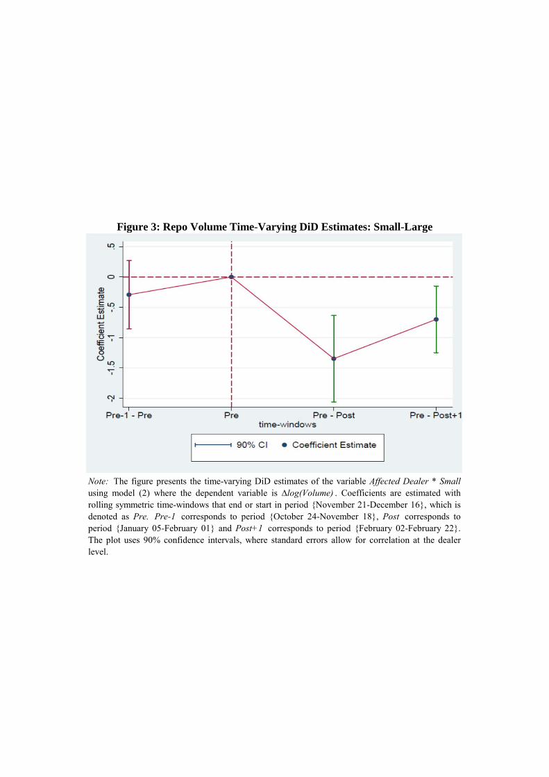
Figure 3: Repo Volume Time-Varying DiD Estimates: Small-Large

Note: The figure presents the time-varying DiD estimates of the variable Affected Dealer * Smallusing model (2) where the dependent variable is ∆log(Volume) . Coefficients are estimated withrolling symmetric time-windows that end or start in period {November 21-December 16}, which isdenoted as Pre. Pre-1 corresponds to period {October 24-November 18}, Post corresponds toperiod {January 05-February 01} and Post+1 corresponds to period {February 02-February 22}.The plot uses 90% confidence intervals, where standard errors allow for correlation at the dealerlevel.

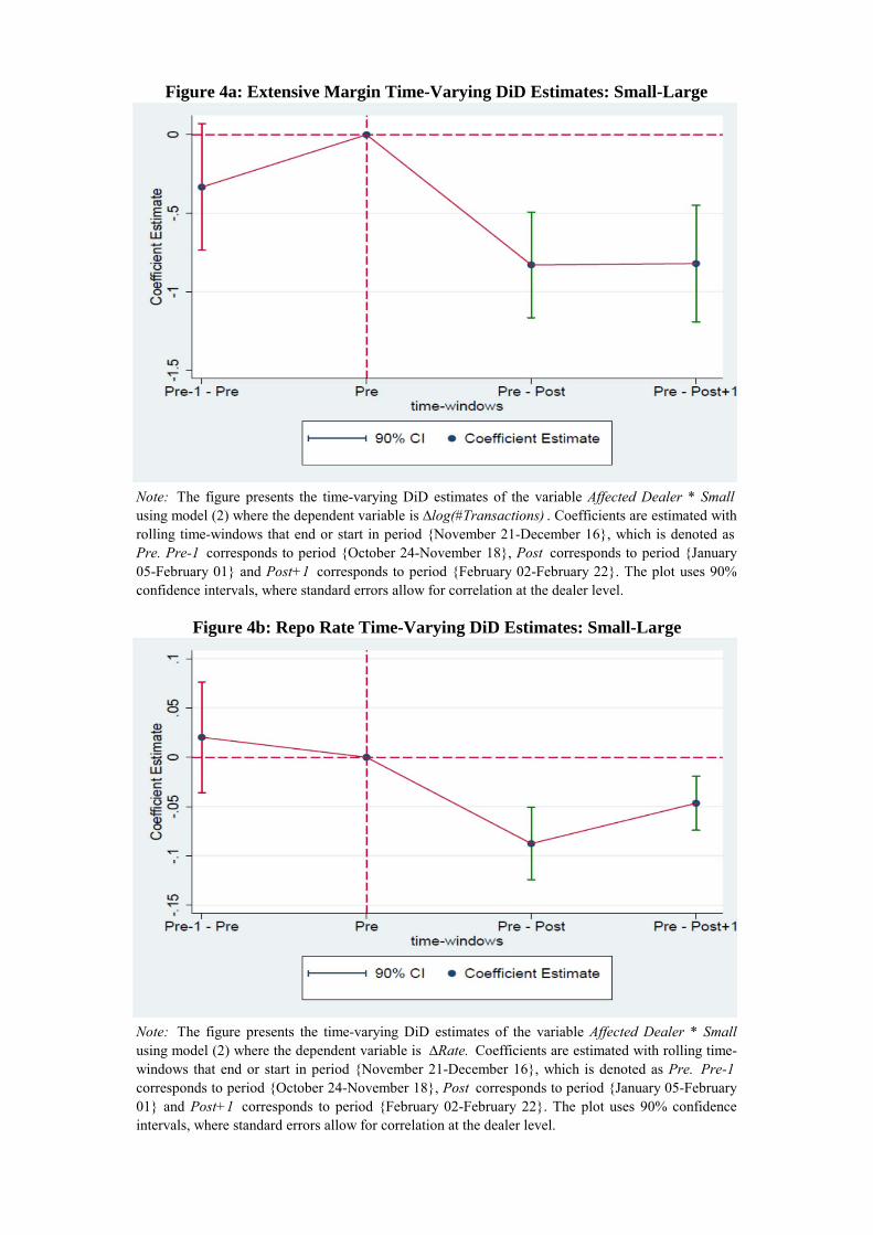
Figure 4a: Extensive Margin Time-Varying DiD Estimates: Small-Large

Note: The figure presents the time-varying DiD estimates of the variable Affected Dealer * Smallusing model (2) where the dependent variable is ∆log(#Transactions) . Coefficients are estimated withrolling time-windows that end or start in period {November 21-December 16}, which is denoted asPre. Pre-1 corresponds to period {October 24-November 18}, Post corresponds to period {January05-February 01} and Post+1 corresponds to period {February 02-February 22}. The plot uses 90%confidence intervals, where standard errors allow for correlation at the dealer level.

Figure 4b: Repo Rate Time-Varying DiD Estimates: Small-Large

Note: The figure presents the time-varying DiD estimates of the variable Affected Dealer * Smallusing model (2) where the dependent variable is ∆Rate. Coefficients are estimated with rolling time-windows that end or start in period {November 21-December 16}, which is denoted as Pre. Pre-1 corresponds to period {October 24-November 18}, Post corresponds to period {January 05-February01} and Post+1 corresponds to period {February 02-February 22}. The plot uses 90% confidenceintervals, where standard errors allow for correlation at the dealer level.

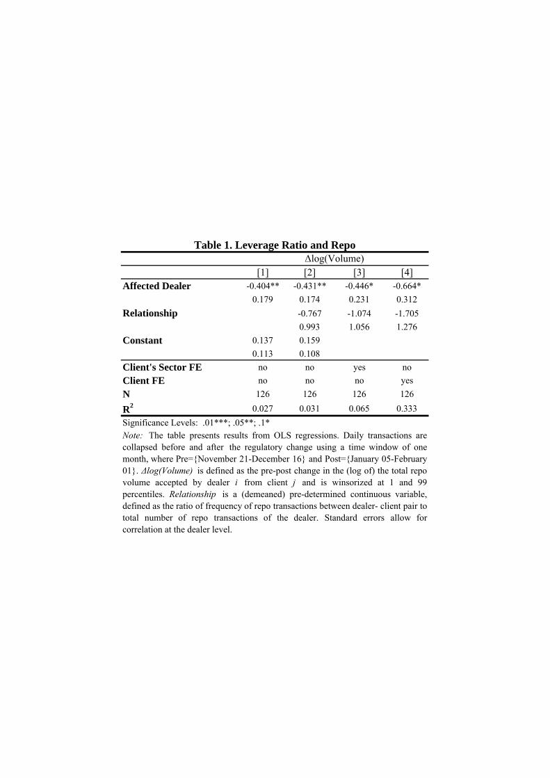
[1] [2] [3] [4]Affected Dealer -0.404** -0.431** -0.446* -0.664*

0.179 0.174 0.231 0.312

Relationship -0.767 -1.074 -1.705

0.993 1.056 1.276

Constant 0.137 0.159

0.113 0.108

Client's Sector FE no no yes no

Client FE no no no yes

N 126 126 126 126

R2 0.027 0.031 0.065 0.333

Significance Levels: .01***; .05**; .1*Note: The table presents results from OLS regressions. Daily transactions arecollapsed before and after the regulatory change using a time window of onemonth, where Pre={November 21-December 16} and Post={January 05-February01}. Δlog(Volume) is defined as the pre-post change in the (log of) the total repovolume accepted by dealer i from client j and is winsorized at 1 and 99percentiles. Relationship is a (demeaned) pre-determined continuous variable,defined as the ratio of frequency of repo transactions between dealer- client pair tototal number of repo transactions of the dealer. Standard errors allow forcorrelation at the dealer level.

Table 1. Leverage Ratio and RepoΔlog(Volume)

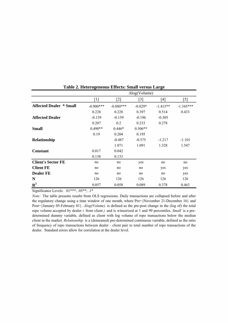
[1] [2] [3] [4] [5]

Affected Dealer * Small -0.900*** -0.880*** -0.829* -1.415** -1.345***

0.228 0.228 0.397 0.514 0.433

Affected Dealer -0.139 -0.159 -0.196 -0.305

0.207 0.2 0.233 0.278

Small 0.490** 0.446* 0.506**

0.19 0.204 0.195

Relationship -0.487 -0.575 -1.217 -1.101

1.071 1.091 1.328 1.547

Constant 0.017 0.042

0.138 0.133

Client's Sector FE no no yes no no

Client FE no no no yes yes

Dealer FE no no no no yes

N 126 126 126 126 126

R2 0.057 0.058 0.089 0.378 0.463

Significance Levels: .01***; .05**; .1*

Δlog(Volume)Table 2. Heterogeneous Effects: Small versus Large

Note: The table presents results from OLS regressions. Daily transactions are collapsed before and afterthe regulatory change using a time window of one month, where Pre={November 21-December 16} andPost={January 05-February 01}. Δlog(Volume) is defined as the pre-post change in the (log of) the totalrepo volume accepted by dealer i from client j and is winsorized at 1 and 99 percentiles. Small is a pre-determined dummy variable, defined as client with log volume of repo transactions below the medianclient in the market. Relationship is a (demeaned) pre-determined continuous variable, defined as the ratioof frequency of repo transactions between dealer - client pair to total number of repo transactions of thedealer. Standard errors allow for correlation at the dealer level.

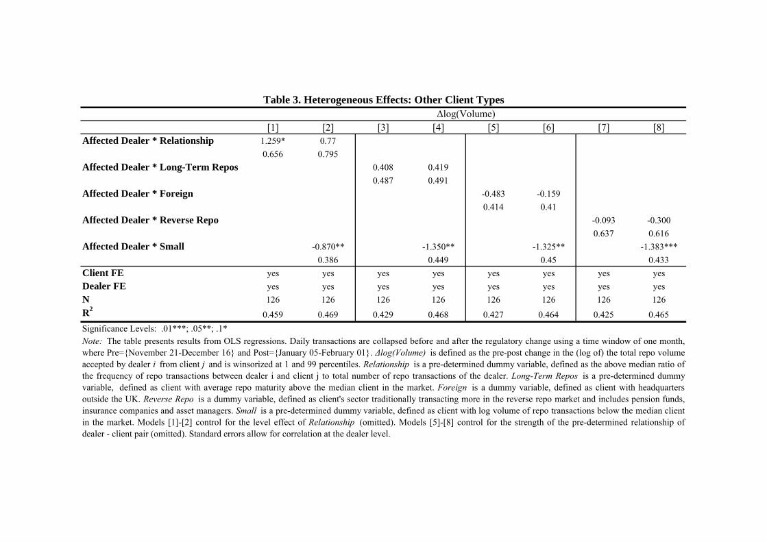
[1] [2] [3] [4] [5] [6] [7] [8]Affected Dealer * Relationship 1.259* 0.77

0.656 0.795

Affected Dealer * Long-Term Repos 0.408 0.419

0.487 0.491

Affected Dealer * Foreign -0.483 -0.159

0.414 0.41

Affected Dealer * Reverse Repo -0.093 -0.300

0.637 0.616

Affected Dealer * Small -0.870** -1.350** -1.325** -1.383***

0.386 0.449 0.45 0.433

Client FE yes yes yes yes yes yes yes yes

Dealer FE yes yes yes yes yes yes yes yes

N 126 126 126 126 126 126 126 126

R20.459 0.469 0.429 0.468 0.427 0.464 0.425 0.465

Significance Levels: .01***; .05**; .1*Note: The table presents results from OLS regressions. Daily transactions are collapsed before and after the regulatory change using a time window of one month,where Pre={November 21-December 16} and Post={January 05-February 01}. Δlog(Volume) is defined as the pre-post change in the (log of) the total repo volumeaccepted by dealer i from client j and is winsorized at 1 and 99 percentiles. Relationship is a pre-determined dummy variable, defined as the above median ratio ofthe frequency of repo transactions between dealer i and client j to total number of repo transactions of the dealer. Long-Term Repos is a pre-determined dummyvariable, defined as client with average repo maturity above the median client in the market. Foreign is a dummy variable, defined as client with headquartersoutside the UK. Reverse Repo is a dummy variable, defined as client's sector traditionally transacting more in the reverse repo market and includes pension funds,insurance companies and asset managers. Small is a pre-determined dummy variable, defined as client with log volume of repo transactions below the median clientin the market. Models [1]-[2] control for the level effect of Relationship (omitted). Models [5]-[8] control for the strength of the pre-determined relationship ofdealer - client pair (omitted). Standard errors allow for correlation at the dealer level.

Table 3. Heterogeneous Effects: Other Client TypesΔlog(Volume)

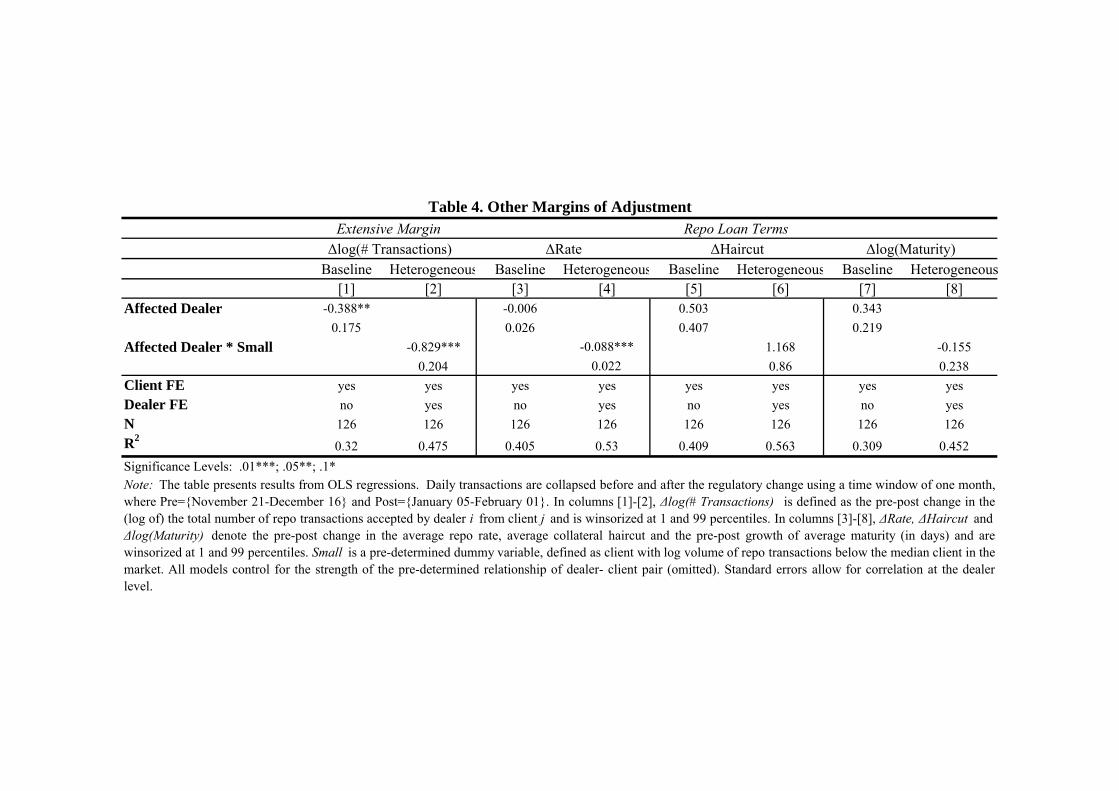
Baseline Heterogeneous Baseline Heterogeneous Baseline Heterogeneous Baseline Heterogeneous[1] [2] [3] [4] [5] [6] [7] [8]

Affected Dealer -0.388** -0.006 0.503 0.343

0.175 0.026 0.407 0.219

Affected Dealer * Small -0.829*** -0.088*** 1.168 -0.155

0.204 0.022 0.86 0.238

Client FE yes yes yes yes yes yes yes yes

Dealer FE no yes no yes no yes no yes

N 126 126 126 126 126 126 126 126

R20.32 0.475 0.405 0.53 0.409 0.563 0.309 0.452

Significance Levels: .01***; .05**; .1*

Table 4. Other Margins of Adjustment

Note: The table presents results from OLS regressions. Daily transactions are collapsed before and after the regulatory change using a time window of one month,where Pre={November 21-December 16} and Post={January 05-February 01}. In columns [1]-[2], Δlog(# Transactions) is defined as the pre-post change in the(log of) the total number of repo transactions accepted by dealer i from client j and is winsorized at 1 and 99 percentiles. In columns [3]-[8], ΔRate, ΔHaircut andΔlog(Maturity) denote the pre-post change in the average repo rate, average collateral haircut and the pre-post growth of average maturity (in days) and arewinsorized at 1 and 99 percentiles. Small is a pre-determined dummy variable, defined as client with log volume of repo transactions below the median client in themarket. All models control for the strength of the pre-determined relationship of dealer- client pair (omitted). Standard errors allow for correlation at the dealerlevel.

ΔHaircutΔlog(# Transactions) ΔRate Δlog(Maturity)Extensive Margin Repo Loan Terms

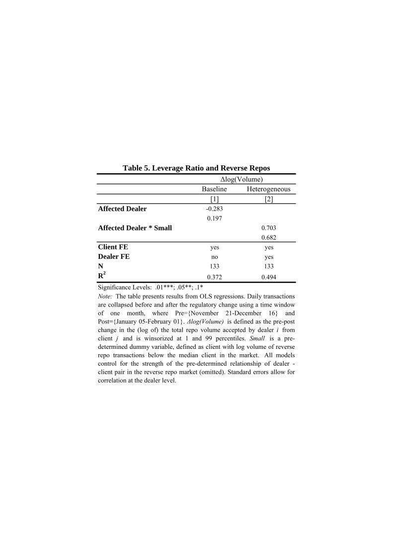
Baseline Heterogeneous[1] [2]

Affected Dealer -0.283

0.197

Affected Dealer * Small 0.703

0.682

Client FE yes yes

Dealer FE no yes

N 133 133

R20.372 0.494

Significance Levels: .01***; .05**; .1*Note: The table presents results from OLS regressions. Daily transactionsare collapsed before and after the regulatory change using a time windowof one month, where Pre={November 21-December 16} andPost={January 05-February 01}. Δlog(Volume) is defined as the pre-postchange in the (log of) the total repo volume accepted by dealer i fromclient j and is winsorized at 1 and 99 percentiles. Small is a pre-determined dummy variable, defined as client with log volume of reverserepo transactions below the median client in the market. All modelscontrol for the strength of the pre-determined relationship of dealer -client pair in the reverse repo market (omitted). Standard errors allow forcorrelation at the dealer level.

Δlog(Volume)

Table 5. Leverage Ratio and Reverse Repos

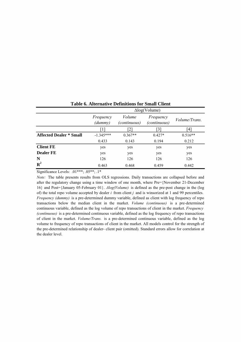
Frequency (dummy)

Volume (continuous)

Frequency (continuous)

Volume/Trans.

[1] [2] [3] [4]Affected Dealer * Small -1.345*** 0.367** 0.427* 0.516**

0.433 0.143 0.194 0.212

Client FE yes yes yes yes

Dealer FE yes yes yes yes

N 126 126 126 126

R20.463 0.468 0.459 0.442

Significance Levels: .01***; .05**; .1*

Table 6. Alternative Definitions for Small ClientΔlog(Volume)

Note: The table presents results from OLS regressions. Daily transactions are collapsed before andafter the regulatory change using a time window of one month, where Pre={November 21-December16} and Post={January 05-February 01}. Δlog(Volume) is defined as the pre-post change in the (logof) the total repo volume accepted by dealer i from client j and is winsorized at 1 and 99 percentiles.Frequency (dummy) is a pre-determined dummy variable, defined as client with log frequency of repotransactions below the median client in the market. Volume (continuous) is a pre-determinedcontinuous variable, defined as the log volume of repo transactions of client in the market. Frequency (continuous) is a pre-determined continuous variable, defined as the log frequency of repo transactionsof client in the market. Volume/Trans. is a pre-determined continuous variable, defined as the logvolume to frequency of repo transactions of client in the market. All models control for the strength ofthe pre-determined relationship of dealer- client pair (omitted). Standard errors allow for correlation atthe dealer level.

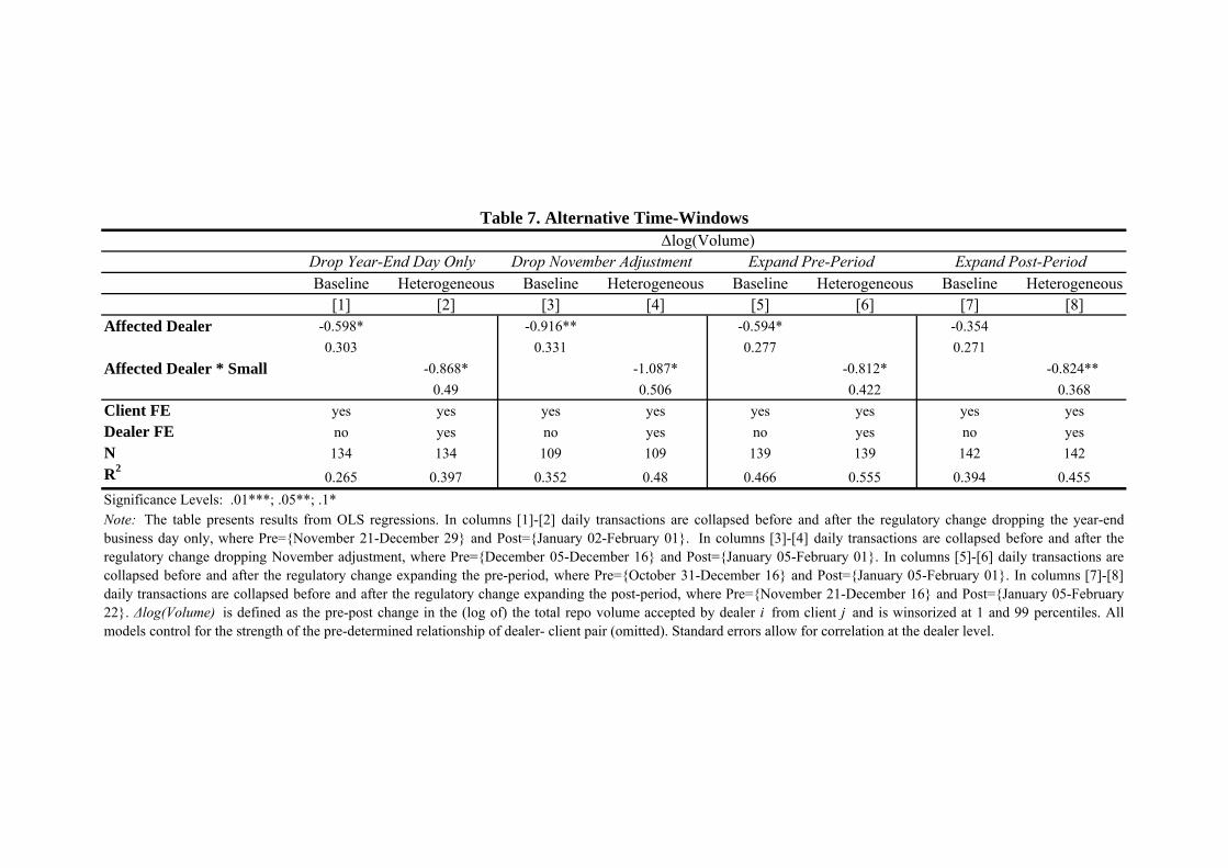
Baseline Heterogeneous Baseline Heterogeneous Baseline Heterogeneous Baseline Heterogeneous[1] [2] [3] [4] [5] [6] [7] [8]

Affected Dealer -0.598* -0.916** -0.594* -0.354

0.303 0.331 0.277 0.271

Affected Dealer * Small -0.868* -1.087* -0.812* -0.824**

0.49 0.506 0.422 0.368

Client FE yes yes yes yes yes yes yes yes

Dealer FE no yes no yes no yes no yes

N 134 134 109 109 139 139 142 142

R20.265 0.397 0.352 0.48 0.466 0.555 0.394 0.455

Significance Levels: .01***; .05**; .1*

Expand Post-Period

Note: The table presents results from OLS regressions. In columns [1]-[2] daily transactions are collapsed before and after the regulatory change dropping the year-endbusiness day only, where Pre={November 21-December 29} and Post={January 02-February 01}. In columns [3]-[4] daily transactions are collapsed before and after theregulatory change dropping November adjustment, where Pre={December 05-December 16} and Post={January 05-February 01}. In columns [5]-[6] daily transactions arecollapsed before and after the regulatory change expanding the pre-period, where Pre={October 31-December 16} and Post={January 05-February 01}. In columns [7]-[8]daily transactions are collapsed before and after the regulatory change expanding the post-period, where Pre={November 21-December 16} and Post={January 05-February22}. Δlog(Volume) is defined as the pre-post change in the (log of) the total repo volume accepted by dealer i from client j and is winsorized at 1 and 99 percentiles. Allmodels control for the strength of the pre-determined relationship of dealer- client pair (omitted). Standard errors allow for correlation at the dealer level.

Table 7. Alternative Time-WindowsΔlog(Volume)

Drop November Adjustment Expand Pre-PeriodDrop Year-End Day Only

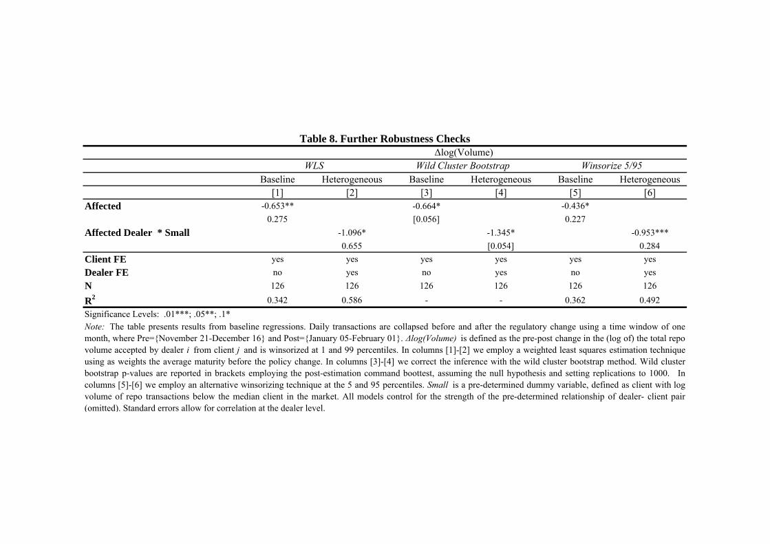
Baseline Heterogeneous Baseline Heterogeneous Baseline Heterogeneous[1] [2] [3] [4] [5] [6]

Affected -0.653** -0.664* -0.436*

0.275 [0.056] 0.227

Affected Dealer * Small -1.096* -1.345* -0.953***

0.655 [0.054] 0.284

Client FE yes yes yes yes yes yes

Dealer FE no yes no yes no yes

N 126 126 126 126 126 126

R2 0.342 0.586 - - 0.362 0.492

Significance Levels: .01***; .05**; .1*

Wild Cluster Bootstrap Winsorize 5/95

Note: The table presents results from baseline regressions. Daily transactions are collapsed before and after the regulatory change using a time window of onemonth, where Pre={November 21-December 16} and Post={January 05-February 01}. Δlog(Volume) is defined as the pre-post change in the (log of) the total repovolume accepted by dealer i from client j and is winsorized at 1 and 99 percentiles. In columns [1]-[2] we employ a weighted least squares estimation techniqueusing as weights the average maturity before the policy change. In columns [3]-[4] we correct the inference with the wild cluster bootstrap method. Wild clusterbootstrap p-values are reported in brackets employing the post-estimation command boottest, assuming the null hypothesis and setting replications to 1000. Incolumns [5]-[6] we employ an alternative winsorizing technique at the 5 and 95 percentiles. Small is a pre-determined dummy variable, defined as client with logvolume of repo transactions below the median client in the market. All models control for the strength of the pre-determined relationship of dealer- client pair(omitted). Standard errors allow for correlation at the dealer level.

Table 8. Further Robustness ChecksΔlog(Volume)

WLS

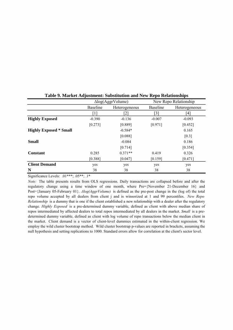
Baseline Heterogeneous Baseline Heterogeneous[1] [2] [3] [4]

Highly Exposed -0.390 -0.136 -0.007 -0.093

[0.273] [0.889] [0.971] [0.452]

Highly Exposed * Small -0.584* 0.165

[0.088] [0.3]

Small -0.084 0.186

[0.714] [0.354]

Constant 0.285 0.371** 0.419 0.326

[0.388] [0.047] [0.159] [0.471]

Client Demand yes yes yes yes

N 38 38 38 38

Significance Levels: .01***; .05**; .1*Note: The table presents results from OLS regressions. Daily transactions are collapsed before and after theregulatory change using a time window of one month, where Pre={November 21-December 16} andPost={January 05-February 01}. Δlog(AggrVolume) is defined as the pre-post change in the (log of) the totalrepo volume accepted by all dealers from client j and is winsorized at 1 and 99 percentiles. New RepoRelationship is a dummy that is one if the client established a new relationship with a dealer after the regulatorychange. Highly Exposed is a pre-determined dummy variable, defined as client with above median share ofrepos intermediated by affected dealers to total repos intermediated by all dealers in the market. Small is a pre-determined dummy variable, defined as client with log volume of repo transactions below the median client inthe market. Client demand is a vector of client-level dummies estimated in the within-client regression. Weemploy the wild cluster bootstrap method. Wild cluster bootstrap p-values are reported in brackets, assuming thenull hypothesis and setting replications to 1000. Standard errors allow for correlation at the client's sector level.

Table 9. Market Adjustment: Substitution and New Repo RelationshipsΔlog(AggrVolume) New Repo Relationship

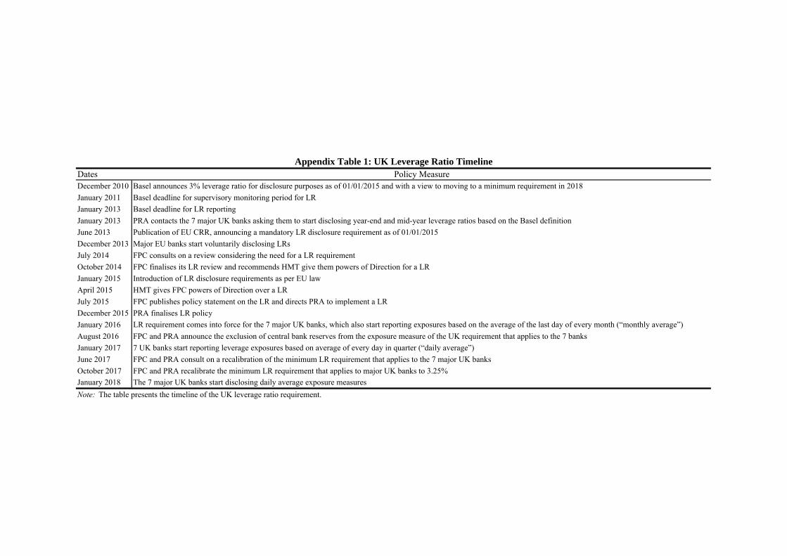
Dates Policy MeasureDecember 2010 Basel announces 3% leverage ratio for disclosure purposes as of 01/01/2015 and with a view to moving to a minimum requirement in 2018

January 2011 Basel deadline for supervisory monitoring period for LR

January 2013 Basel deadline for LR reporting

January 2013 PRA contacts the 7 major UK banks asking them to start disclosing year-end and mid-year leverage ratios based on the Basel definition

June 2013 Publication of EU CRR, announcing a mandatory LR disclosure requirement as of 01/01/2015

December 2013 Major EU banks start voluntarily disclosing LRs

July 2014 FPC consults on a review considering the need for a LR requirement

October 2014 FPC finalises its LR review and recommends HMT give them powers of Direction for a LR

January 2015 Introduction of LR disclosure requirements as per EU law

April 2015 HMT gives FPC powers of Direction over a LR

July 2015 FPC publishes policy statement on the LR and directs PRA to implement a LR

December 2015 PRA finalises LR policy

January 2016 LR requirement comes into force for the 7 major UK banks, which also start reporting exposures based on the average of the last day of every month (“monthly average”)

August 2016 FPC and PRA announce the exclusion of central bank reserves from the exposure measure of the UK requirement that applies to the 7 banks

January 2017 7 UK banks start reporting leverage exposures based on average of every day in quarter (“daily average”)

June 2017 FPC and PRA consult on a recalibration of the minimum LR requirement that applies to the 7 major UK banks

October 2017 FPC and PRA recalibrate the minimum LR requirement that applies to major UK banks to 3.25%

January 2018 The 7 major UK banks start disclosing daily average exposure measures

Appendix Table 1: UK Leverage Ratio Timeline

Note: The table presents the timeline of the UK leverage ratio requirement.

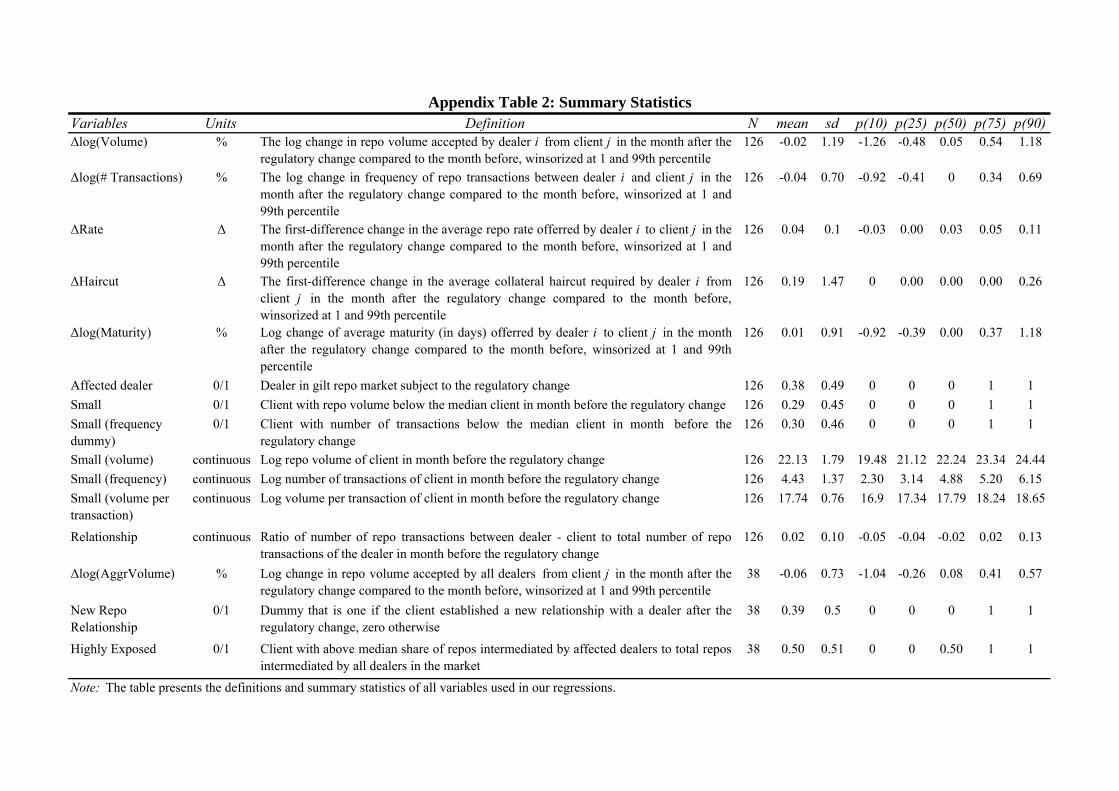
Variables Units Definition N mean sd p(10) p(25) p(50) p(75) p(90)Δlog(Volume) % The log change in repo volume accepted by dealer i from client j in the month after the

regulatory change compared to the month before, winsorized at 1 and 99th percentile126 -0.02 1.19 -1.26 -0.48 0.05 0.54 1.18

Δlog(# Transactions) % The log change in frequency of repo transactions between dealer i and client j in themonth after the regulatory change compared to the month before, winsorized at 1 and99th percentile

126 -0.04 0.70 -0.92 -0.41 0 0.34 0.69

ΔRate Δ The first-difference change in the average repo rate offerred by dealer i to client j in themonth after the regulatory change compared to the month before, winsorized at 1 and99th percentile

126 0.04 0.1 -0.03 0.00 0.03 0.05 0.11

ΔHaircut Δ The first-difference change in the average collateral haircut required by dealer i fromclient j in the month after the regulatory change compared to the month before,winsorized at 1 and 99th percentile

126 0.19 1.47 0 0.00 0.00 0.00 0.26

Δlog(Maturity) % Log change of average maturity (in days) offerred by dealer i to client j in the monthafter the regulatory change compared to the month before, winsorized at 1 and 99thpercentile

126 0.01 0.91 -0.92 -0.39 0.00 0.37 1.18

Affected dealer 0/1 Dealer in gilt repo market subject to the regulatory change 126 0.38 0.49 0 0 0 1 1

Small 0/1 Client with repo volume below the median client in month before the regulatory change 126 0.29 0.45 0 0 0 1 1

Small (frequency dummy)

0/1 Client with number of transactions below the median client in month before theregulatory change

126 0.30 0.46 0 0 0 1 1

Small (volume) continuous Log repo volume of client in month before the regulatory change 126 22.13 1.79 19.48 21.12 22.24 23.34 24.44

Small (frequency) continuous Log number of transactions of client in month before the regulatory change 126 4.43 1.37 2.30 3.14 4.88 5.20 6.15

Small (volume per transaction)

continuous Log volume per transaction of client in month before the regulatory change 126 17.74 0.76 16.9 17.34 17.79 18.24 18.65

Relationship continuous Ratio of number of repo transactions between dealer - client to total number of repotransactions of the dealer in month before the regulatory change

126 0.02 0.10 -0.05 -0.04 -0.02 0.02 0.13

Δlog(AggrVolume) % Log change in repo volume accepted by all dealers from client j in the month after theregulatory change compared to the month before, winsorized at 1 and 99th percentile

38 -0.06 0.73 -1.04 -0.26 0.08 0.41 0.57

New Repo Relationship

0/1 Dummy that is one if the client established a new relationship with a dealer after theregulatory change, zero otherwise

38 0.39 0.5 0 0 0 1 1

Highly Exposed 0/1 Client with above median share of repos intermediated by affected dealers to total reposintermediated by all dealers in the market

38 0.50 0.51 0 0 0.50 1 1

Note: The table presents the definitions and summary statistics of all variables used in our regressions.

Appendix Table 2: Summary Statistics