Repeater Amplifier Systems:Principles and Applications

Seminar Subjects

by Ernesto A. Alcivar

SYSTEMSINC.

SYSTEMSINC.

© 1994 TX RX Systems Inc. C2012J94V2.0

INTRODUCTIONDefinition

Repeater amplifiers, also known as signal boosters, are specialized RF systems that extend radiocoverage into enclosed or shadowed areas where abrupt propagation losses impair communication.Materials such as soil or rock, brick, cement, reinforced concrete, metals, and metal-coated thermalglass panes are notorious for their ability to block electromagnetic radiation in the radio frequencyrange. In the interior of structures made of those materials, and in areas where natural or man-madestructures block radio propagation, radio frequency levels may be 30 to 100 dB or more below unob-structed levels (nothing but cosmic ray particles and neutrinos penetrates into deep mines, for exam-ple). Repeater amplifiers boost radio signals to levels sufficiently high to provide reliablecommunication in those enclosed or blocked areas.

Historical BackgroundRepeater amplifiers have acquired great prominence in the radio communication industry in the

last few years, due to a rapidly growing demand for extended communications services inside alltypes of urban structures. However, they made their first appearances several decades ago, as a partof "leaky feeder" or "leaky coax" radio communication systems in underground mines, vehicular andrailroad tunnels. One-way repeater amplifiers were used in various configurations for simplex andsemiduplex radio communication in underground tunnels. Two-way repeater amplifiers appearedmore recently, and TX RX Systems Inc. has played a significant role in their development.

TX RX Systems Inc. was the first manufacturer of fully integrated, two-way repeater amplifiersystems in the U.S. The first UHF two-way repeater amplifiers were manufactured in 1978, in re-sponse to a requirement by Motorola Communications. They were subsequently installed in anInland Steel Corporation coal mine in Illinois, where they continue to provide reliable undergroundradio communication to this day. Since then, thousands of TX RX Systems' repeater amplifiers havebeen sold for private, commercial, government and military applications that include paging, radio-telephone, trunking and two-way radio systems in the frequency range from 66 to beyond 960 MHz.

TX RX Systems' repeater amplifiers have been used in such places as:The construction phase of the English Channel Tunnel or "Chunnel" (few people know that 140VHF two-way repeater amplifiers manufactured by TX RX Systems Inc. were used in the sys-tem described in references 5 and 20)O'Hare International Airport in ChicagoNew York Port Authority facilitiesThe San Francisco Bay Area Rapid Transit System (BART)The King Fahd International Airport in Saudi ArabiaSubway stations in Lyon, FranceMany commercial high-rise buildings, shopping centers, manufacturing plants and hospitals inthe U.S.Vehicular tunnels in TaiwanNuclear and hydroelectric power plants in the U.S.The Cook County Jail in IllinoisThe largest copper mine in the world in ChileThe subway system in Caracas, Venezuela

Key to TX RX Systems' long-term success has been its proven ability to solve tough applicationproblems and provide substantive system engineering support to its customers. The quality andbreadth of its engineering support is, in fact, a key element that has consistently differentiated TXRX Systems from its competitors.

Page 1 Lit. No. C20012J94

About This BookletThis booklet, a part of TX RX Systems' long-standing Seminar Subjects series, presents a broad

but concise overview of repeater amplifier systems and design methods. Our motives for writing thismaterial are twofold.

First, the best published technical articles on the subject have either provided exquisite technicaldetail on specific system implementations, or have provided highly theoretical discussions of nar-rowly specialized subjects. Lesser published articles fall in the category of marketing narrativeswhich describe the great success of specific products in their peculiar applications, without providingmuch technical insight ("We put three of our Model XYZ amplifiers in a vehicular tunnel and re-duced dropped cellular calls by 90%", etc.) To acquire a basic familiarity with the broad subject of re-peater amplifier systems, the interested system engineer must locate and read many articles,textbooks and technical papers published over the last four decades or so. It is very difficult to put to-gether a coherent mental picture of a multidisciplinary field, based on brief glimpses into unfamiliarsubjects. The list of references at the end of this booklet includes only a small fraction of the manybooks, technical papers and articles that contain relevant information. Busy professionals in our sec-tor of the industry may not have the time and motivation to engage in literature research of the kindrequired.

Second, prospective repeater amplifier customers frequently spend many hours in conversationwith our engineering and sales personnel, in a process that eventually leads to our understanding ofthe application and the customer's understanding of the technology required to solve the communica-tion problem. We take great pride in our ability to provide technical support, but we have long feltthat we would rather spend long hours either analyzing our customer's application in ways thatleave nothing to the imagination, or fine-tuning the system design to maximize the probability of mu-tual satisfaction.

Prospective repeater amplifier customers often wonder why we ask so many questions when theyinquire about our products. After all, they just want a quick quotation on a specific repeater amplifiermodel number, right?. It turns out that every application parameter, from the frequency plan to thelocation of radios and antennas within the system, has a profound effect on how the hardware shouldbe configured. We will have achieved a worthwhile objective if the material below succeeds in ex-plaining why we need so much information to quote one bit of equipment.

We have divided the material into four self-contained but closely related parts:Repeater Amplifier Basics provides an introduction to repeater amplifiers and their basiccomponents, without engaging in too much technical discussion, for the benefit of those whowish to quickly familiarize themselves with the subject.Repeater Amplifier Applications provides a brief overview of how repeater amplifiers areused to provide radio communication coverage in blocked or enclosed areas.Amplifier Noise, Intermodulation and Dynamic Range provides a practical compendiumof technical facts about linear amplifiers, including formulas, tabulations and graphs that weuse in our daily work for purposes of repeater amplifier system design.Repeater Amplifier System Architecture puts it all together: it discusses a repeater ampli-fier system design example, emphasizing how the system configuration has been calculated tosatisfy application requirements.

Page 2 Lit. No. C20012J94

PART I - REPEATER AMPLIFIER BASICSDefinition of Non-Heterodyne (Broadband) Repeater Amplifier

Non-heterodyne (broadband) repeater amplifiers utilize linear amplifiers with input and outputfilters that restrict pass bandwidth to a specified frequency range. No frequency conversion processesare involved in their operation. Filter pass bandwidth may range from 25 KHz at VHF to 25 MHz atGSM cellular frequencies. Non-heterodyne amplifiers are generally less complex and expensive thanheterodyne (channelized) repeater amplifiers. They therefore provide a cost-effective solution to awide variety of communication problems.

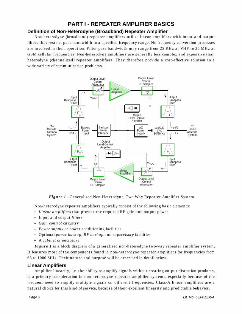
Non-heterodyne repeater amplifiers typically consist of the following basic elements: Linear amplifiers that provide the required RF gain and output powerInput and output filtersGain control circuitryPower supply or power conditioning facilitiesOptional power backup, RF backup and supervisory facilitiesA cabinet or enclosure

Figure 1 is a block diagram of a generalized non-heterodyne two-way repeater amplifier system.It features most of the components found in non-heterodyne repeater amplifiers for frequencies from66 to 1000 MHz. Their nature and purpose will be described in detail below.

Linear AmplifiersAmplifier linearity, i.e. the ability to amplify signals without creating output distortion products,

is a primary consideration in non-heterodyne repeater amplifier systems, especially because of thefrequent need to amplify multiple signals on different frequencies. Class-A linear amplifiers are anatural choice for this kind of service, because of their excellent linearity and predictable behavior.

Page 3 Lit. No. C20012J94

VAGC

VAGC

Output LevelControl

Attenuator

BackupPowerInput

115/230VAC

50/60 Hz

InputBandpass

Filter

OutputBandpassFilter

Output LevelControl

RF Sampler

OutputLevel Control

Amplifier

Output LevelControl

Attenuator

Output LevelControl

RF Sampler

InputBandpassFilter

OutputBandpass

Filter

RF

F1

F2

F1

F2

RF

ToOutsideAntennaSystem

ToInside

AntennaSystem

OutputLevel Control

Amplifier

LinearAmpllifier

F1 F1

BackupPower

Interface

ACPowerSupply

F2F2

LinearAmpllifier

Figure 1 - Generalized Non-Heterodyne, Two-Way Repeater Amplifier System

TX RX Systems' linear amplifier stages have typical gains from +12 to more than +20 dB and1-dB output compression points of a few hundred milliwatts to six watts. Output intercept points arein the range of +23 to +49 dBm, depending on the type and frequency range of the amplifier. Noisefigure ranges from less than 2 dB in low-noise, low-level stages, to 10 dB in high-power stages.Broadband amplifiers are not required, as operating bandwidths rarely exceed 1% to 3% of centerfrequency.

Repeater amplifier systems may have one, two or more amplifier branches, one for each directionof signal transmission and/or frequency range. The gain, pass bandwidth, center frequency and out-put power of each branch may be completely different from each other. Low-noise, medium- andhigh-power stages can be combined in various ways to obtain optimum RF output power, noise figureand intermodulation characteristics.

Because the integrity of an entire communication system depends on reliable amplifier perform-ance, careful attention must be paid to the choice of active devices. TX RX Systems utilizes linear bi-polar devices of the highest quality and reliability. They are operated well within the manufacturer'srecommended limits. High-level amplifiers are outfitted with heatsinks of ample dimensions to keepsemiconductor junction temperatures well below maximum ratings.

FiltersFilters perform important functions in repeater amplifier systems. In one-way systems, input fil-

ters reject undesired signals to minimize the potential for interference, and output filters attenuateout-of-band amplifier noise and spuria. In two-way systems, the input and output filters on adjacentamplifier branches also provide selectivity well in excess of total amplifier gain at all frequencies, inorder to assure unconditional amplifier stability. In repeater amplifiers with more than two amplifierbranches, stable operation can only be achieved with filter designs that provide sufficient isolationbetween all possible branch pairs.

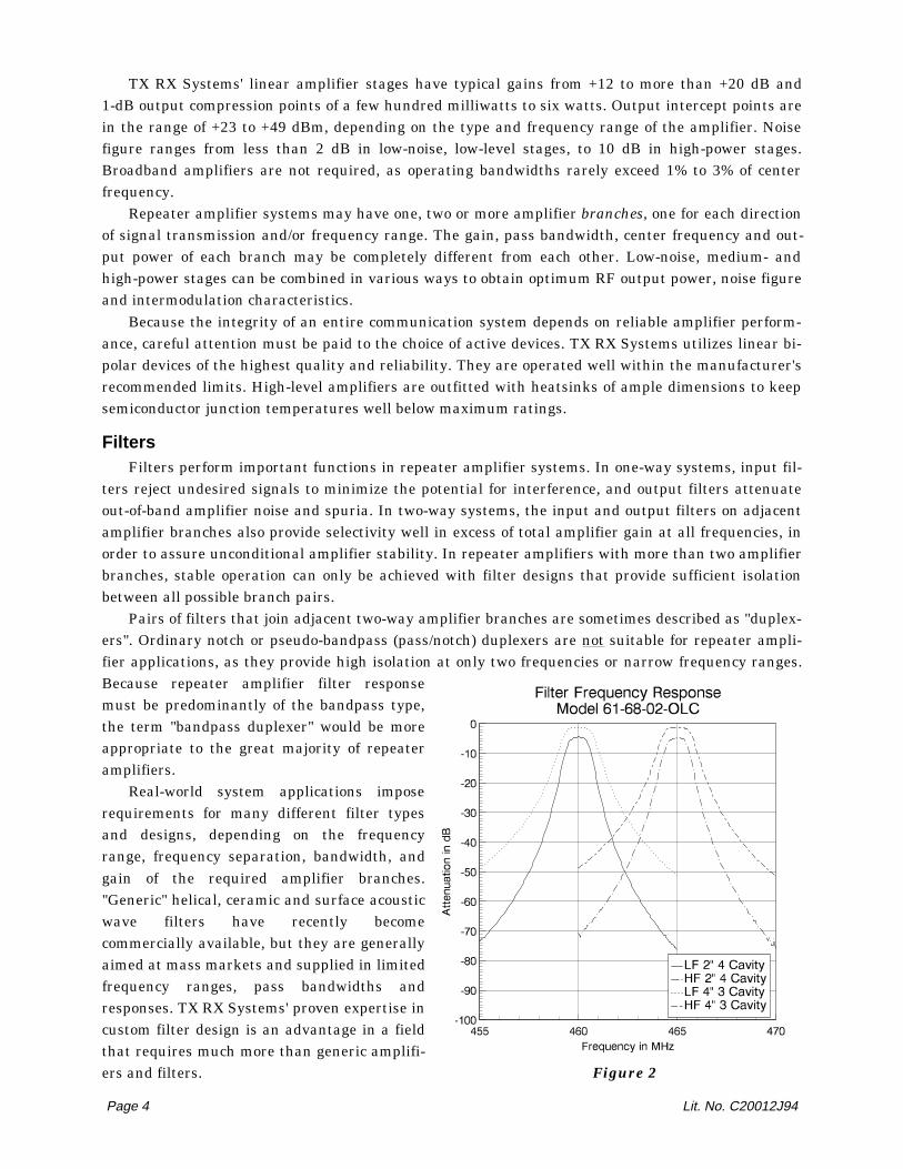
Pairs of filters that join adjacent two-way amplifier branches are sometimes described as "duplex-ers". Ordinary notch or pseudo-bandpass (pass/notch) duplexers are not suitable for repeater ampli-fier applications, as they provide high isolation at only two frequencies or narrow frequency ranges.Because repeater amplifier filter responsemust be predominantly of the bandpass type,the term "bandpass duplexer" would be moreappropriate to the great majority of repeateramplifiers.

Real-world system applications imposerequirements for many different filter typesand designs, depending on the frequencyrange, frequency separation, bandwidth, andgain of the required amplifier branches."Generic" helical, ceramic and surface acousticwave filters have recently becomecommercially available, but they are generallyaimed at mass markets and supplied in limitedfrequency ranges, pass bandwidths andresponses. TX RX Systems' proven expertise incustom filter design is an advantage in a fieldthat requires much more than generic amplifi-ers and filters.

Page 4 Lit. No. C20012J94

Figure 2

Figure 2 shows the frequency response of the bandpass filters used in repeater amplifier Model61-68-02-OLC. A block diagram of the system is shown in Figure 3. The two curves centered on460.0 MHz are the response of the low-frequency passband input (lower curve) and output (uppercurve) filters. The two curves centered on 465.0 MHz are the response of the high-frequency pass-band input and output filters. The input filter assemblies are 4-section, aperture-coupled designsutilizing 2" square 1/4-wave resonators. They provide excellent selectivity at moderate insertion loss,in a relatively compact package. Typical insertion loss is in the order of -4.7 dB at the center fre-quency. Typical pass bandwidth is ±0.4 MHz at -5.7 dB insertion loss. It is important to minimizeoutput filter insertion loss, in order to minimize the degradation of amplifier output power and third-order intercept point. Because of this, the branch output filters consist of three loop-coupled, 4" quar-terwave cavities which provide satisfactory selectivity at an insertion loss of only -1.3 dB at the filtercenter frequency. Pass bandwidth is ±0.4 MHz at -1.6 dB insertion loss.

Isolation between the high- and low-frequency passbands at a specified frequency is the sum offilter selectivity at that frequency. Minimum isolation occurs at the upper edge of the lower passbandand at the lower edge of the upper passband. In this case in particular, minimum isolation is -122.3dB at 460.4 MHz (-5.7-68.4-1.5-46.7 dB). If a conservative isolation margin of 12 dB is allowed for am-plifier stability at all frequencies, the sum of high- and low-frequency amplifier gain should not behigher than +110.3 dB. This particular filter configuration is therefore suitable for UHF repeater am-plifier systems operating at minimum T-R separations of 5 MHz, at a gain of not more than 55 dB perbranch. Amplifier gain in Model 61-68-02-OLC is approximately 48 dB per branch.

Bandpass filters made with TX RX Systems' 4-inch diameter quarterwave cavities, such as thethree-cavity filter described above, are an excellent choice for VHF and UHF repeater amplifierwork. Two to four cavities may be used to accommodate different bandwidth and selectivity require-ments. Adjustable loops make it easy to set the selectivity of individual cavities as required to obtaina specified frequency response.

Page 5 Lit. No. C20012J94

3W

Base Tx

3-Cavity4" Bandpass F ilter

+21 VDC

+15 VDC

Detector

+24 VDC

117 VAC60 Hz

AC Power Supply

To BatteryBackup M odule

+24VDC

+21 VDC

+15 VDC

Detector

+24 VDC

-50 dBSampler

Portable Tx

RFPad

RFPad

3-Cavity4" Bandpass Filter

Base Tx O utPortable Tx In

Base Tx InPortable Tx O ut

Dual DCRegulator

Dual DCRegulator

OpAmp

OpAmp

4-Cavity Iris-Coup led2" Bandpass Filter

4-Cavity Iris-Coupled2" Bandpass Filter

-50 dBSampler

Figure 3 - Model 61-68-02-OLC Repeater Amplifier System

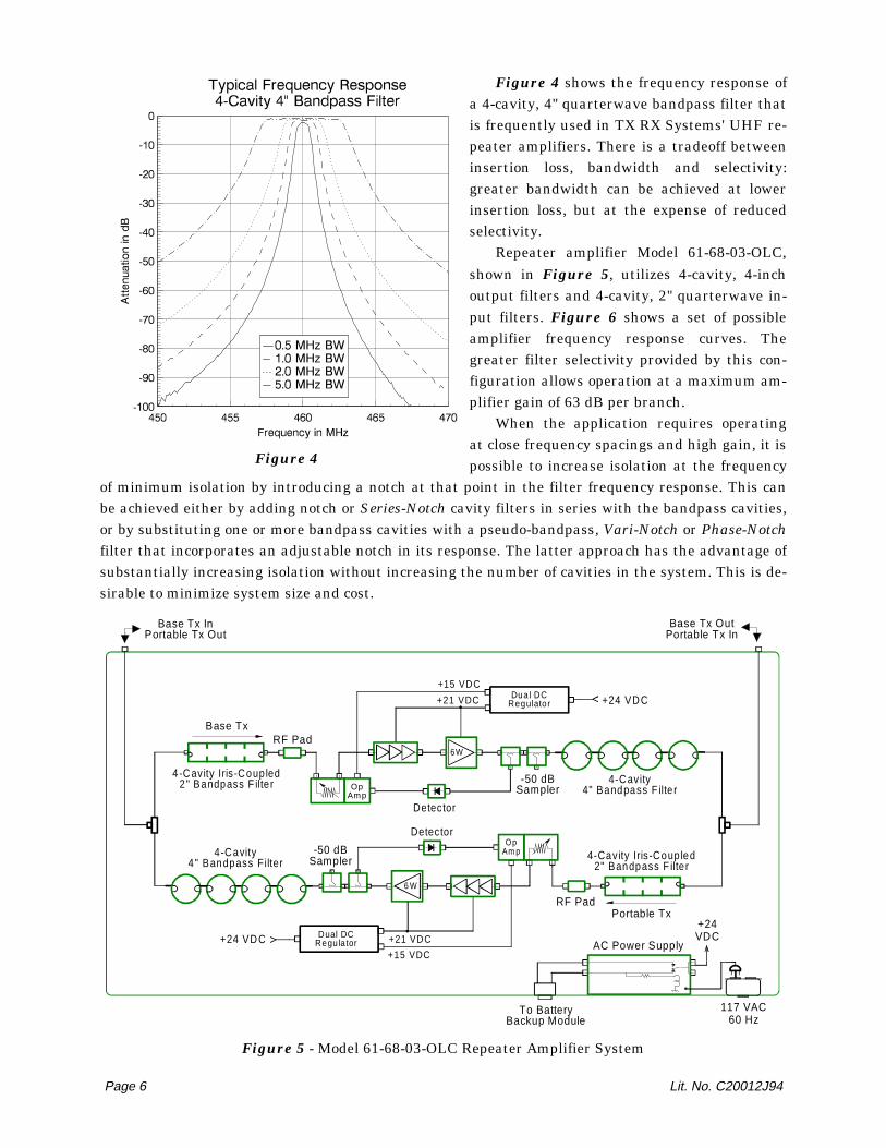
Figure 4 shows the frequency response ofa 4-cavity, 4" quarterwave bandpass filter thatis frequently used in TX RX Systems' UHF re-peater amplifiers. There is a tradeoff betweeninsertion loss, bandwidth and selectivity:greater bandwidth can be achieved at lowerinsertion loss, but at the expense of reducedselectivity.

Repeater amplifier Model 61-68-03-OLC,shown in Figure 5, utilizes 4-cavity, 4-inchoutput filters and 4-cavity, 2" quarterwave in-put filters. Figure 6 shows a set of possibleamplifier frequency response curves. Thegreater filter selectivity provided by this con-figuration allows operation at a maximum am-plifier gain of 63 dB per branch.

When the application requires operatingat close frequency spacings and high gain, it ispossible to increase isolation at the frequency

of minimum isolation by introducing a notch at that point in the filter frequency response. This canbe achieved either by adding notch or Series-Notch cavity filters in series with the bandpass cavities,or by substituting one or more bandpass cavities with a pseudo-bandpass, Vari-Notch or Phase-Notchfilter that incorporates an adjustable notch in its response. The latter approach has the advantage ofsubstantially increasing isolation without increasing the number of cavities in the system. This is de-sirable to minimize system size and cost.

Page 6 Lit. No. C20012J94

Figure 4

Figure 5 - Model 61-68-03-OLC Repeater Amplifier System

6 W

4-Cavity4" Bandpass Filter

+21 VDC

+15 VDC

Detector

+24 VDC

117 VAC60 Hz

AC Power Supply

To BatteryBackup Module

+24VDC

-50 dBSampler

Portable TxRF Pad

Base Tx InPortable Tx Out

Base Tx OutPortable Tx In

4-Cavity Iris-Coup led2" Bandpass F ilte r

4-Cavity4" Bandpass F ilte r

+21 VDC

+15 VDC

Detector

+24 VDC

-50 dBSampler

Base TxRF Pad

4-Cavity Iris-Coup led2" Bandpass F ilte r

6W

Dual DCRegulator

Dual DCRegulator

OpAmp

OpAm p

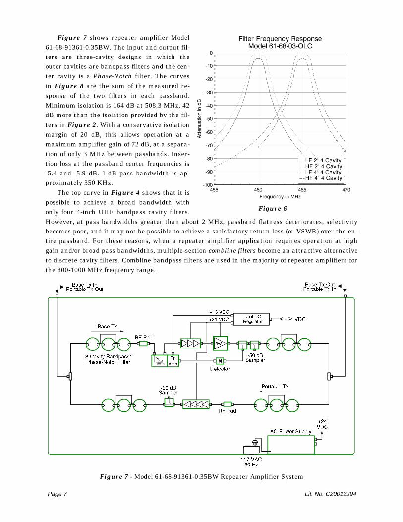
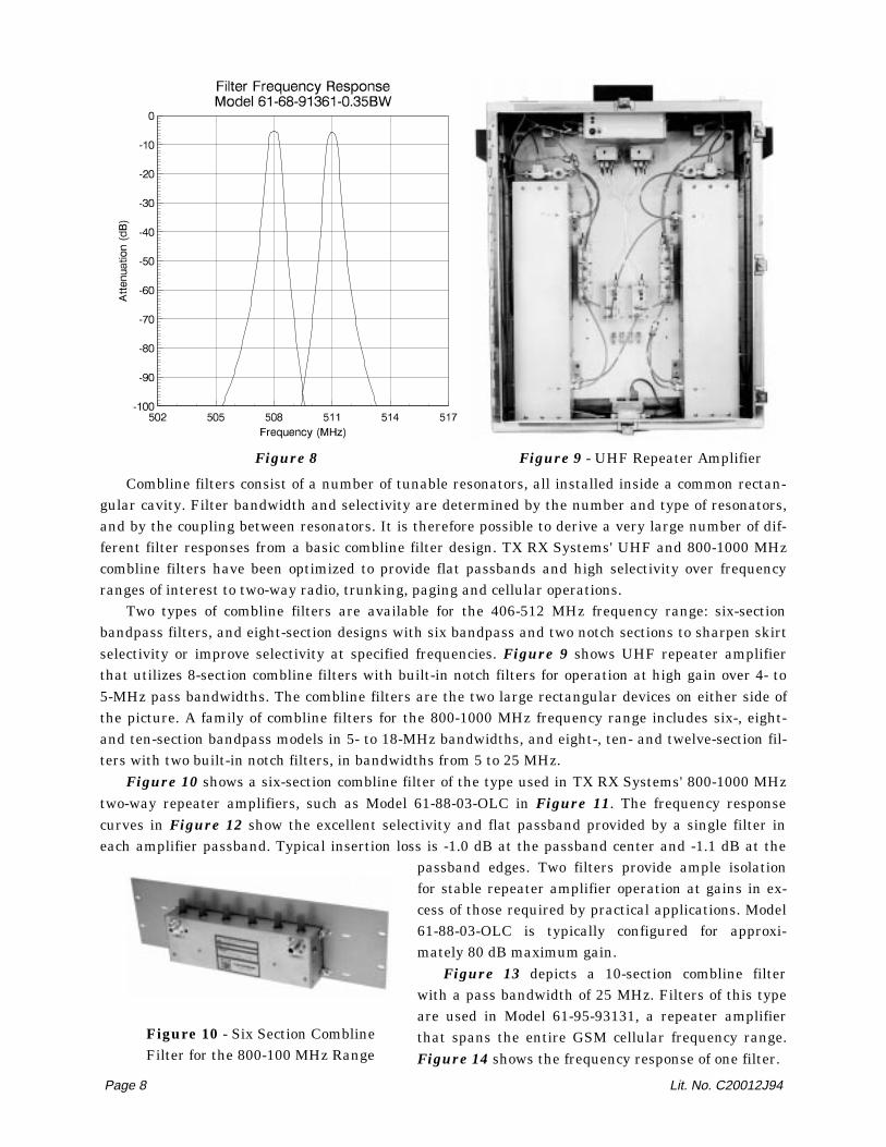
Figure 7 shows repeater amplifier Model61-68-91361-0.35BW. The input and output fil-ters are three-cavity designs in which theouter cavities are bandpass filters and the cen-ter cavity is a Phase-Notch filter. The curvesin Figure 8 are the sum of the measured re-sponse of the two filters in each passband.Minimum isolation is 164 dB at 508.3 MHz, 42dB more than the isolation provided by the fil-ters in Figure 2. With a conservative isolationmargin of 20 dB, this allows operation at amaximum amplifier gain of 72 dB, at a separa-tion of only 3 MHz between passbands. Inser-tion loss at the passband center frequencies is-5.4 and -5.9 dB. 1-dB pass bandwidth is ap-proximately 350 KHz.

The top curve in Figure 4 shows that it ispossible to achieve a broad bandwidth withonly four 4-inch UHF bandpass cavity filters.However, at pass bandwidths greater than about 2 MHz, passband flatness deteriorates, selectivitybecomes poor, and it may not be possible to achieve a satisfactory return loss (or VSWR) over the en-tire passband. For these reasons, when a repeater amplifier application requires operation at highgain and/or broad pass bandwidths, multiple-section combline filters become an attractive alternativeto discrete cavity filters. Combline bandpass filters are used in the majority of repeater amplifiers forthe 800-1000 MHz frequency range.

Page 7 Lit. No. C20012J94

Figure 6

Figure 7 - Model 61-68-91361-0.35BW Repeater Amplifier System

Combline filters consist of a number of tunable resonators, all installed inside a common rectan-gular cavity. Filter bandwidth and selectivity are determined by the number and type of resonators,and by the coupling between resonators. It is therefore possible to derive a very large number of dif-ferent filter responses from a basic combline filter design. TX RX Systems' UHF and 800-1000 MHzcombline filters have been optimized to provide flat passbands and high selectivity over frequencyranges of interest to two-way radio, trunking, paging and cellular operations.

Two types of combline filters are available for the 406-512 MHz frequency range: six-sectionbandpass filters, and eight-section designs with six bandpass and two notch sections to sharpen skirtselectivity or improve selectivity at specified frequencies. Figure 9 shows UHF repeater amplifierthat utilizes 8-section combline filters with built-in notch filters for operation at high gain over 4- to5-MHz pass bandwidths. The combline filters are the two large rectangular devices on either side ofthe picture. A family of combline filters for the 800-1000 MHz frequency range includes six-, eight-and ten-section bandpass models in 5- to 18-MHz bandwidths, and eight-, ten- and twelve-section fil-ters with two built-in notch filters, in bandwidths from 5 to 25 MHz.

Figure 10 shows a six-section combline filter of the type used in TX RX Systems' 800-1000 MHztwo-way repeater amplifiers, such as Model 61-88-03-OLC in Figure 11. The frequency responsecurves in Figure 12 show the excellent selectivity and flat passband provided by a single filter ineach amplifier passband. Typical insertion loss is -1.0 dB at the passband center and -1.1 dB at the

passband edges. Two filters provide ample isolationfor stable repeater amplifier operation at gains in ex-cess of those required by practical applications. Model61-88-03-OLC is typically configured for approxi-mately 80 dB maximum gain.

Figure 13 depicts a 10-section combline filterwith a pass bandwidth of 25 MHz. Filters of this typeare used in Model 61-95-93131, a repeater amplifierthat spans the entire GSM cellular frequency range.Figure 14 shows the frequency response of one filter.

Page 8 Lit. No. C20012J94

Figure 8

Figure 10 - Six Section ComblineFilter for the 800-100 MHz Range

Figure 9 - UHF Repeater Amplifier

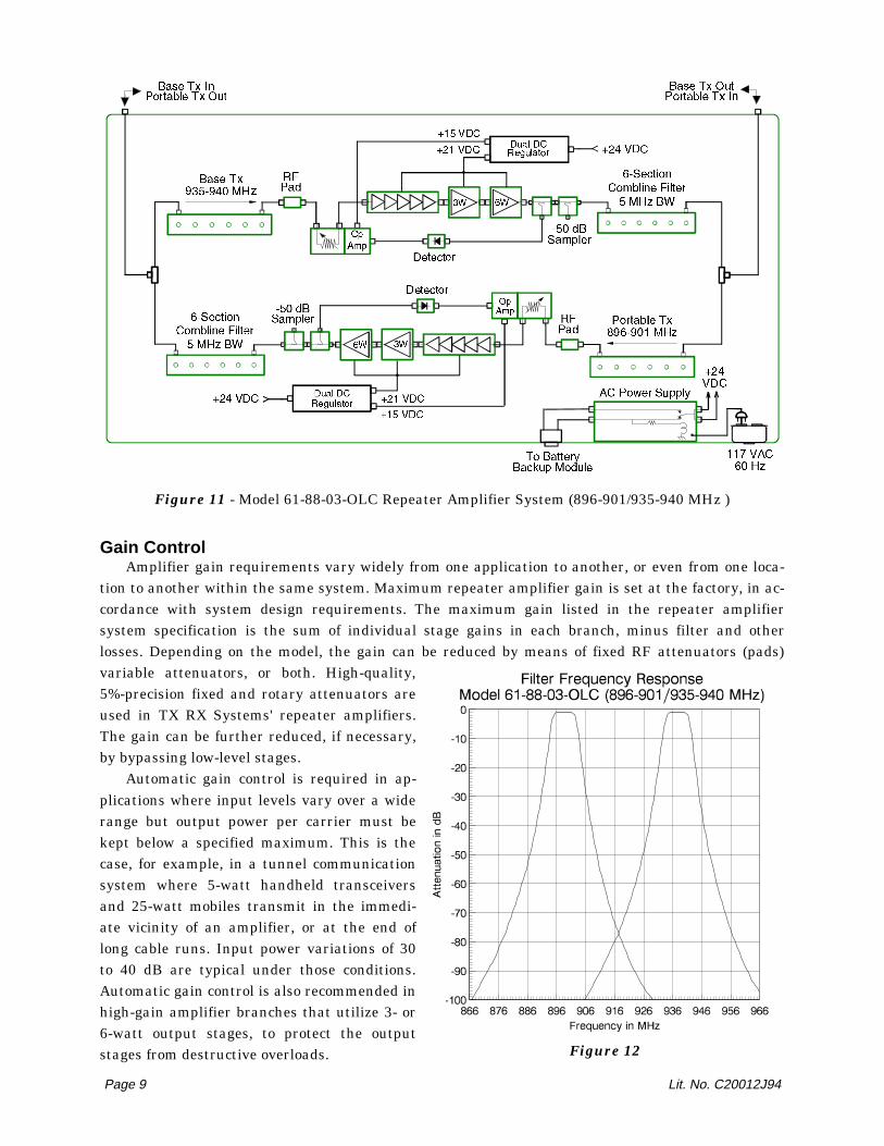
Gain ControlAmplifier gain requirements vary widely from one application to another, or even from one loca-

tion to another within the same system. Maximum repeater amplifier gain is set at the factory, in ac-cordance with system design requirements. The maximum gain listed in the repeater amplifiersystem specification is the sum of individual stage gains in each branch, minus filter and otherlosses. Depending on the model, the gain can be reduced by means of fixed RF attenuators (pads)variable attenuators, or both. High-quality,5%-precision fixed and rotary attenuators areused in TX RX Systems' repeater amplifiers.The gain can be further reduced, if necessary,by bypassing low-level stages.

Automatic gain control is required in ap-plications where input levels vary over a widerange but output power per carrier must bekept below a specified maximum. This is thecase, for example, in a tunnel communicationsystem where 5-watt handheld transceiversand 25-watt mobiles transmit in the immedi-ate vicinity of an amplifier, or at the end oflong cable runs. Input power variations of 30to 40 dB are typical under those conditions.Automatic gain control is also recommended inhigh-gain amplifier branches that utilize 3- or6-watt output stages, to protect the outputstages from destructive overloads.

Page 9 Lit. No. C20012J94

Figure 11 - Model 61-88-03-OLC Repeater Amplifier System (896-901/935-940 MHz )

Figure 12

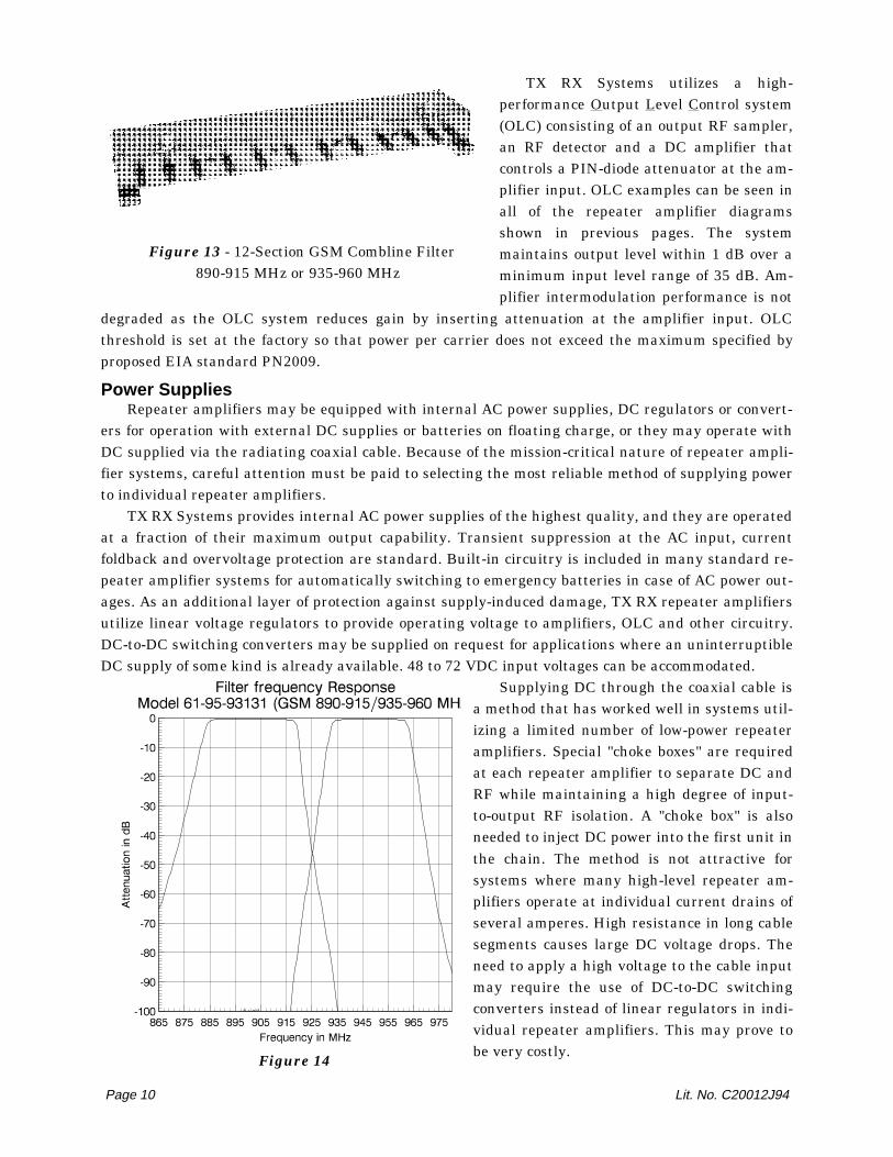
TX RX Systems utilizes a high-performance Output Level Control system(OLC) consisting of an output RF sampler,an RF detector and a DC amplifier thatcontrols a PIN-diode attenuator at the am-plifier input. OLC examples can be seen inall of the repeater amplifier diagramsshown in previous pages. The systemmaintains output level within 1 dB over aminimum input level range of 35 dB. Am-plifier intermodulation performance is not

degraded as the OLC system reduces gain by inserting attenuation at the amplifier input. OLCthreshold is set at the factory so that power per carrier does not exceed the maximum specified byproposed EIA standard PN2009.

Power SuppliesRepeater amplifiers may be equipped with internal AC power supplies, DC regulators or convert-

ers for operation with external DC supplies or batteries on floating charge, or they may operate withDC supplied via the radiating coaxial cable. Because of the mission-critical nature of repeater ampli-fier systems, careful attention must be paid to selecting the most reliable method of supplying powerto individual repeater amplifiers.

TX RX Systems provides internal AC power supplies of the highest quality, and they are operatedat a fraction of their maximum output capability. Transient suppression at the AC input, currentfoldback and overvoltage protection are standard. Built-in circuitry is included in many standard re-peater amplifier systems for automatically switching to emergency batteries in case of AC power out-ages. As an additional layer of protection against supply-induced damage, TX RX repeater amplifiersutilize linear voltage regulators to provide operating voltage to amplifiers, OLC and other circuitry.DC-to-DC switching converters may be supplied on request for applications where an uninterruptibleDC supply of some kind is already available. 48 to 72 VDC input voltages can be accommodated.

Supplying DC through the coaxial cable isa method that has worked well in systems util-izing a limited number of low-power repeateramplifiers. Special "choke boxes" are requiredat each repeater amplifier to separate DC andRF while maintaining a high degree of input-to-output RF isolation. A "choke box" is alsoneeded to inject DC power into the first unit inthe chain. The method is not attractive forsystems where many high-level repeater am-plifiers operate at individual current drains ofseveral amperes. High resistance in long cablesegments causes large DC voltage drops. Theneed to apply a high voltage to the cable inputmay require the use of DC-to-DC switchingconverters instead of linear regulators in indi-vidual repeater amplifiers. This may prove tobe very costly.

Page 10 Lit. No. C20012J94

Figure 13 - 12-Section GSM Combline Filter890-915 MHz or 935-960 MHz

Figure 14

Supervisory and Backup FacilitiesA reasonable degree of system monitoring

is desirable, but common sense dictates thatfault prevention is a more worthwhile invest-ment than sophisticated fault detection andreporting. For example, the failure of a singlepower supply may put an entire system out ofcommission. It would make much more senseto operate repeater amplifiers with externaltelecommunication grade batteries on floatingcharge, instead of using elaborate A/D con-verters, microprocessors and modems to reporttemperatures, voltages, currents and, ulti-mately, system failures. The 8-bit industrial microprocessor is a fine technological achievement, butusing it for inappropriate purposes is not necessarily good engineering. TX RX Systems' experienceindicates that the probability of low-level amplifier failure is astronomically small. Therefore itmakes little sense to increase system cost with low-level stage monitoring facilities. Besides, monitor-ing amplifier RF output power, VSWR and system signal integrity requires complicated transponder,intermittent carrier or pilot carrier monitoring arrangements.

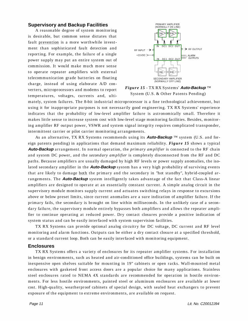
As an alternative, TX RX Systems recommends using its Auto-Backup ™ system (U.S. and for-eign patents pending) in applications that demand maximum reliability. Figure 15 shows a typicalAuto-Backup arrangement. In normal operation, the primary amplifier is connected to the RF chainand system DC power, and the secondary amplifier is completely disconnected from the RF and DCpaths. Because amplifiers are usually damaged by high RF levels or power supply anomalies, the iso-lated secondary amplifier in the Auto-Backup system has a very high probability of surviving eventsthat are likely to damage both the primary and the secondary in "hot standby", hybrid-coupled ar-rangements. The Auto-Backup system intelligently takes advantage of the fact that Class-A linearamplifiers are designed to operate at an essentially constant current. A simple analog circuit in thesupervisory module monitors supply current and actuates switching relays in response to excursionsabove or below preset limits, since current anomalies are a sure indication of amplifier failure. If theprimary fails, the secondary is brought on line within milliseconds. In the unlikely case of a secon-dary failure, the supervisory module entirely bypasses both amplifiers and allows the repeater ampli-fier to continue operating at reduced power. Dry contact closures provide a positive indication ofsystem status and can be easily interfaced with system supervision facilities.

TX RX Systems can provide optional analog circuitry for DC voltage, DC current and RF levelmonitoring and alarm functions. Outputs can be either a dry contact closure at a specified threshold,or a standard current loop. Both can be easily interfaced with monitoring equipment.

EnclosuresTX RX Systems offers a variety of enclosures for its repeater amplifier systems. For installation

in benign environments, such as heated and air-conditioned office buildings, systems can be built oninexpensive open shelves suitable for mounting in 19" cabinets or open racks. Wall-mounted metalenclosures with gasketed front access doors are a popular choice for many applications. Stainlesssteel enclosures rated to NEMA 4X standards are recommended for operation in hostile environ-ments. For less hostile environments, painted steel or aluminum enclosures are available at lowercost. High-quality, weatherproof cabinets of special design, with sealed heat exchangers to preventexposure of the equipment to extreme environments, are available on request.

Page 11 Lit. No. C20012J94

6W3W

DC1IN OUTDC2

DC1IN OUTDC2

6W3W

PRIMARY AMPLIFIER(NORMALLY ON LINE)

SECONDARY AMPLIFIER(NORMALLY OFF LINE)

+21VDC

RF OUTPUTRF INPUT

ALARM OUTPUTS

Figure 15 - TX RX Systems' Auto-Backup ™System (U.S. & Other Patents Pending)

PART II - REPEATER AMPLIFIER APPLICATIONS

Repeater amplifier system applications can be grouped into three different categories:Type I: Tunnels.Type II: Buildings or enclosed structures.Type III: Shadowed areas behind high terrain or structures.

The above categories cover a wide variety of specific applications ranging from high-rise officebuildings to aircraft carriers. The difference lies in the type of signal distribution system utilized toprovide radio coverage inside the enclosed or blocked area.

TYPE I APPLICATIONS: TUNNELS

General DescriptionTunnels are long, narrow underground or interior spaces, bounded by lossy materials such as re-

inforced concrete, soil, rock or others. The following spaces belong in this category:Mine access shafts and tunnelsHydroelectric plant shafts and ductsRailway and vehicular tunnels, the "Chunnel" being the longest by farLong passageways in airport terminals and commercial buildingsUnderground transportation system tunnels (metros, subways, etc.)

Radio Signals in TunnelsRadio signals do not propagate well in narrow tunnels bounded by lossy walls. Attempts at cou-

pling 30 to 960 MHz radio signals into tunnels by means of antennas have typically resulted in longi-tudinal propagation ranging from poor to very bad. For this reason, "leaky feeder" systems,consisting of transmission lines that are deliberately made to radiate along their length, have beendeveloped to generate relatively uniform RF fields inside tunnels. At low frequencies (30-50 or 66-88MHz), transmission line longitudinal loss is small and it is feasible to provide communication insidelong tunnels with relatively small input RF power. At higher frequencies, however, transmission lineloss severely limits communication range, and the brute-force application of high RF power maycause problems of a different kind.

Page 12 Lit. No. C20012J94

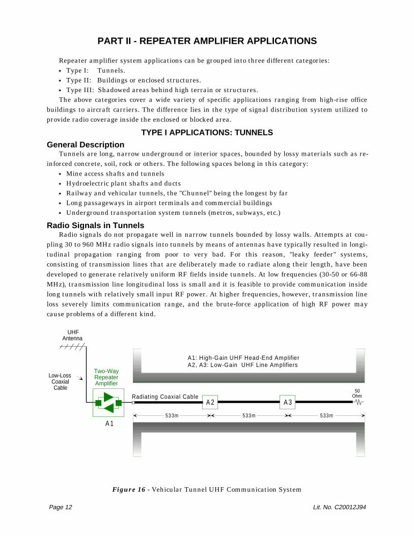
Figure 16 - Vehicular Tunnel UHF Communication System

A1: High-Gain UHF Head-End AmplifierA2, A3: Low-Gain UHF Line Amplifiers

UHFAntenna

A 1

A 3Radiating Coaxial Cable

Low-LossCoaxialCable

A 2

Two-WayRepeaterAmplifier

50Ohm

53 3m 533m533m

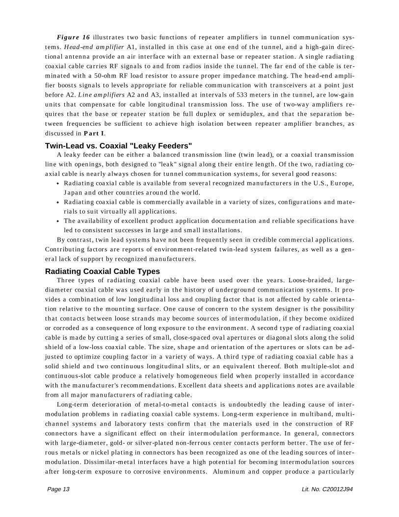
Figure 16 illustrates two basic functions of repeater amplifiers in tunnel communication sys-tems. Head-end amplifier A1, installed in this case at one end of the tunnel, and a high-gain direc-tional antenna provide an air interface with an external base or repeater station. A single radiatingcoaxial cable carries RF signals to and from radios inside the tunnel. The far end of the cable is ter-minated with a 50-ohm RF load resistor to assure proper impedance matching. The head-end ampli-fier boosts signals to levels appropriate for reliable communication with transceivers at a point justbefore A2. Line amplifiers A2 and A3, installed at intervals of 533 meters in the tunnel, are low-gainunits that compensate for cable longitudinal transmission loss. The use of two-way amplifiers re-quires that the base or repeater station be full duplex or semiduplex, and that the separation be-tween frequencies be sufficient to achieve high isolation between repeater amplifier branches, asdiscussed in Part I.

Twin-Lead vs. Coaxial "Leaky Feeders"A leaky feeder can be either a balanced transmission line (twin lead), or a coaxial transmission

line with openings, both designed to "leak" signal along their entire length. Of the two, radiating co-axial cable is nearly always chosen for tunnel communication systems, for several good reasons:

Radiating coaxial cable is available from several recognized manufacturers in the U.S., Europe,Japan and other countries around the world.Radiating coaxial cable is commercially available in a variety of sizes, configurations and mate-rials to suit virtually all applications.The availability of excellent product application documentation and reliable specifications haveled to consistent successes in large and small installations.

By contrast, twin lead systems have not been frequently seen in credible commercial applications.Contributing factors are reports of environment-related twin-lead system failures, as well as a gen-eral lack of support by recognized manufacturers.

Radiating Coaxial Cable TypesThree types of radiating coaxial cable have been used over the years. Loose-braided, large-

diameter coaxial cable was used early in the history of underground communication systems. It pro-vides a combination of low longitudinal loss and coupling factor that is not affected by cable orienta-tion relative to the mounting surface. One cause of concern to the system designer is the possibilitythat contacts between loose strands may become sources of intermodulation, if they become oxidizedor corroded as a consequence of long exposure to the environment. A second type of radiating coaxialcable is made by cutting a series of small, close-spaced oval apertures or diagonal slots along the solidshield of a low-loss coaxial cable. The size, shape and orientation of the apertures or slots can be ad-justed to optimize coupling factor in a variety of ways. A third type of radiating coaxial cable has asolid shield and two continuous longitudinal slits, or an equivalent thereof. Both multiple-slot andcontinuous-slot cable produce a relatively homogeneous field when properly installed in accordancewith the manufacturer's recommendations. Excellent data sheets and applications notes are availablefrom all major manufacturers of radiating cable.

Long-term deterioration of metal-to-metal contacts is undoubtedly the leading cause of inter-modulation problems in radiating coaxial cable systems. Long-term experience in multiband, multi-channel systems and laboratory tests confirm that the materials used in the construction of RFconnectors have a significant effect on their intermodulation performance. In general, connectorswith large-diameter, gold- or silver-plated non-ferrous center contacts perform better. The use of fer-rous metals or nickel plating in connectors has been recognized as one of the leading sources of inter-modulation. Dissimilar-metal interfaces have a high potential for becoming intermodulation sourcesafter long-term exposure to corrosive environments. Aluminum and copper produce a particularly

Page 13 Lit. No. C20012J94

bad electrolytic pair. Therefore, there is a valid reason for concern about the reliability of connectorjoints on radiating cable made with an aluminum shield. However, field experience indicates thatsilver-plated connector bodies and proper connector waterproofing techniques go a long way towardspreventing long-term problems, regardless of the type of cable or connectors. Also, properly-designedconnectors utilize attachment methods that produce high-pressure, inherently hermetic metal-to-metal interfaces.

Feeding the Radiating Cable SystemRadiating cable systems can be either connected directly to base station radios or repeaters in the

tunnel or its vicinity, or they may operate with remote base stations or repeaters radios via air inter-faces or optical fiber links. Each method has its advantages and disadvantages.

I. Base Station Radios in TunnelsOn superficial examination, it appears that coupling high-power base transmitters and high-

sensitivity receivers into a radiating cable system could be a cost-effective system solution, as satis-factory signal levels can be achieved without amplification over considerable cable lengths. However,there are two drawbacks:

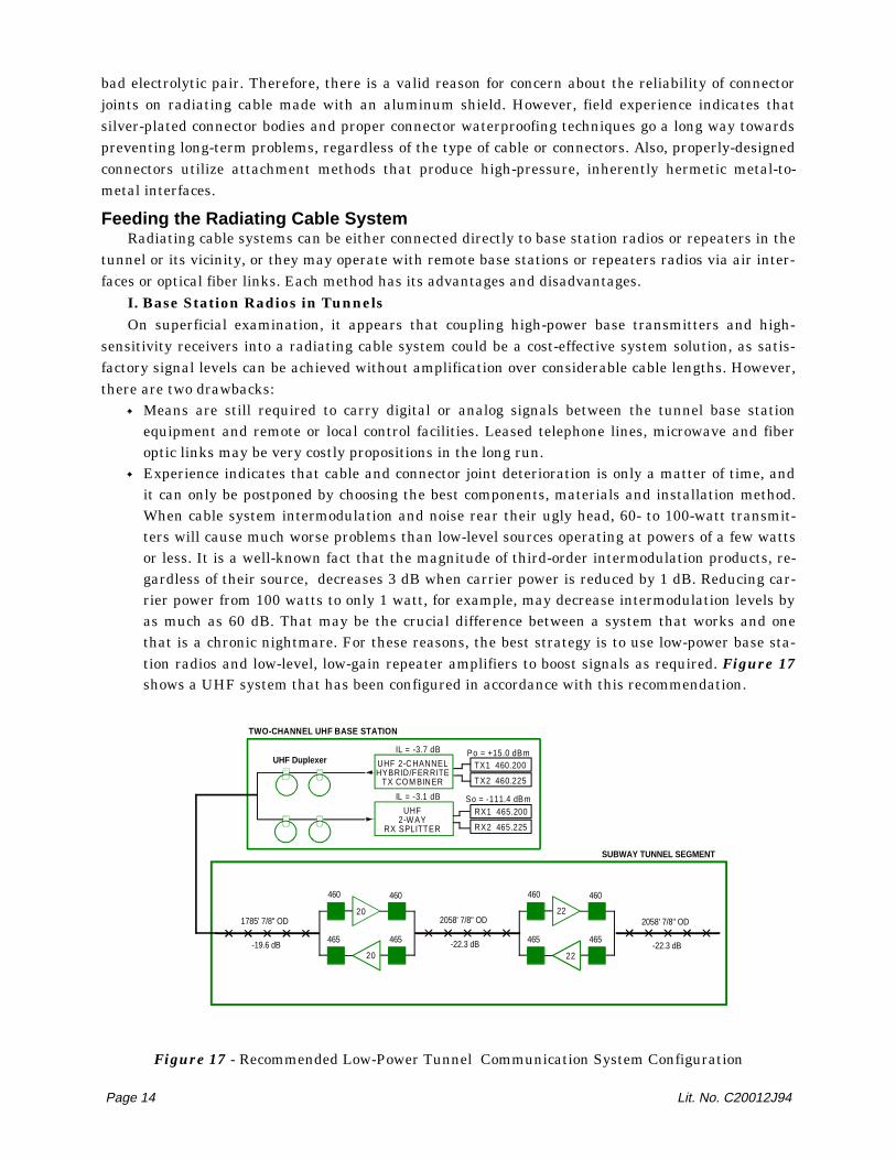
Means are still required to carry digital or analog signals between the tunnel base stationequipment and remote or local control facilities. Leased telephone lines, microwave and fiberoptic links may be very costly propositions in the long run. Experience indicates that cable and connector joint deterioration is only a matter of time, andit can only be postponed by choosing the best components, materials and installation method.When cable system intermodulation and noise rear their ugly head, 60- to 100-watt transmit-ters will cause much worse problems than low-level sources operating at powers of a few wattsor less. It is a well-known fact that the magnitude of third-order intermodulation products, re-gardless of their source, decreases 3 dB when carrier power is reduced by 1 dB. Reducing car-rier power from 100 watts to only 1 watt, for example, may decrease intermodulation levels byas much as 60 dB. That may be the crucial difference between a system that works and onethat is a chronic nightmare. For these reasons, the best strategy is to use low-power base sta-tion radios and low-level, low-gain repeater amplifiers to boost signals as required. Figure 17shows a UHF system that has been configured in accordance with this recommendation.

Page 14 Lit. No. C20012J94

SUBWAY TUNNEL SEGMENT

TWO-CHANNEL UHF BASE STATION

IL = -3.1 dB So = -111.4 dBmUHF

2-W AYRX SPLITTER

Po = +15.0 dBmIL = -3.7 dB

UHF 2-C HANNELHYBRID/FER RITE

TX COM BIN ER

TX1 460.200

TX2 460.225

RX1 465.200

RX2 465.225

1785' 7/8" OD

-19.6 dB

20

460 460

20

465 465

22

460 460

22

465 465

2058' 7/8" OD

-22.3 dB

2058' 7/8" OD

-22.3 dB

UHF Duplexer

Figure 17 - Recommended Low-Power Tunnel Communication System Configuration

II. Air Interface with Base Station RadiosAn air interface is often the most economical way to provide radio signals in a tunnel, as it does

not require additional radio equipment or the high cost of installing it inside the tunnel. The tunnelsystem depicted in Figure 16 and the in-building system in Figure 19 utilize air interfaces with ex-ternal system base stations or repeaters. The head-end repeater amplifier provides bidirectional am-plification for signals traveling from the base station to the radios inside the tunnel or building(downlink) and in the opposite direction (uplink).

Air interfaces work best when base transmitter power and propagation loss to the head-end am-plifier are such that repeater amplifier input signal levels exceed -70 to -90 dBm. Reliable operationat lower levels may not be possible, depending on site noise, fading margins, repeater amplifier noisefloor and other system design considerations. Using high-gain antennas at the head-end repeater am-plifier site is always advantageous, as each decibel of antenna gain reduces amplifier gain and dy-namic range requirements by an equal amount. Decibel for decibel, antenna gain may be lessexpensive than amplifier gain and may reduce amplifier dynamic range requirements.

III. Fiber Optic InterfaceFiber optic technology has advanced to the point that off-the-shelf transmitters and receivers for

broadband RF transmission are available from several sources. Complete links have been specificallyoptimized for operation at relatively high levels with multiple carriers, as required, for example, fortrunking radio and cellular radiotelephone system service.

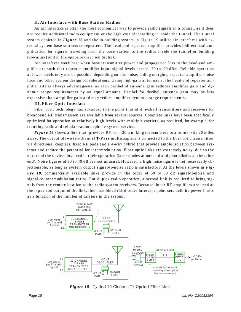
Figure 18 shows a link that provides RF from 20 trunking transmitters to a tunnel site 20 milesaway. The output of two ten-channel T-Pass multicouplers is connected to the fiber optic transmittervia directional couplers, fixed RF pads and a 4-way hybrid that provide ample isolation between sys-tems and reduce the potential for intermodulation. Fiber optic links are extremely noisy, due to thenature of the devices involved in their operation (laser diodes at one end and photodiodes at the otherend). Noise figures of 30 to 40 dB are not unusual. However, a high noise figure is not necessarily ob-jectionable, as long as system output signal-to-noise ratio is satisfactory. At the levels shown in Fig-ure 18, commercially available links provide in the order of 50 to 60 dB signal-to-noise andsignal-to-intermodulation ratios. For duplex radio operation, a second link is required to bring sig-nals from the remote location to the radio system receivers. Because linear RF amplifiers are used atthe input and output of the link, their combined third-order intercept point sets definite power limitsas a function of the number of carriers in the system.

Page 15 Lit. No. C20012J94

Figure 18 - Typical 20-Channel Tx Optical Fiber Link

TYPICAL 24 W(+43.8 dBm)

PER CARRIER

50-OHML OAD

-20 dBP A D

50-OHML OAD

-20 dBP A D

1

1 0

1 1

2 0

-30 dBDECOUPLER

-30 dBDECOUPLER

FIBER-OPTICXM TR

4-WAYHYBRID

COUPLERFIBER-OPTICR C V R

100 Wattsper Channel

Typical

100 Wattsper Channel

Typical

-6 .2 dBTYP ICAL

OPTICAL FIBER

~ -14 dB TOTAL LOSS(includ ing 20 Km optical

fiber and connectors)

~ -27 dBmper Carrier

10-CHANNELT-PASS

TRANSMITTERMULTICOUPLER

10-CHANNELT-PASS

TRANSMITTERMULTICOUPLER

Fiber optic link manufacturers often talk about the low cost of optical fiber ("pennies per foot!") asone of the significant advantages of their technology. By the time optical fibers are wrapped in pro-tective layers suitable for burial or exposure to weather, the cost of fiber optic cable has risen to lev-els comparable to low-loss coaxial cable. Furthermore, the cost of installing optical fiber cable caneasily be in the order of tens of thousands of dollars per mile, and there may be significant right-of-way problems. As of this writing, the cost of one-way fiber optic links is still in the order of manythousands of dollars, and other RF link technologies may be far more attractive from the standpointof total installed cost. The main advantage of fiber optic technology lies in its phenomenal bandwidthand information carrying capacity. As a means to carry thousands of data or voice channels, it maybe quite reasonably priced. As a means to carry only a few narrowband RF channels, it may be tooexpensive for practical purposes.

Type II Applications: BuildingsBuildings require three-dimensional signal distribution systems to provide coverage in relatively

open spaces, narrow corridors, staircases and ventilation or elevator shafts. A high-gain, head-endrepeater amplifier usually provides an interface between an external radio system and the interior ofthe building. In large building complexes with many users (hospitals or large factories, for example),it may be preferable to use an internal, dedicated base station to provide communication service tousers in the facility. Two-way line amplifiers may then be required to overcome signal distributionlosses within the complex.

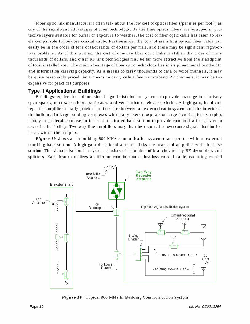
Figure 19 shows an in-building 800 MHz communication system that operates with an externaltrunking base station. A high-gain directional antenna links the head-end amplifier with the basestation. The signal distribution system consists of a number of branches fed by RF decouplers andsplitters. Each branch utilizes a different combination of low-loss coaxial cable, radiating coaxial

Page 16 Lit. No. C20012J94

800 MH zAntenna

To Low erF loors

R FD ecoupler

R adiating Coaxia l C able

Low-Loss Coaxial Cable

E levator Shaft

4-WayDivider

OmnidirectionalAntenna

Top Floor Signal Distribution System

YagiAntenna

Two-WayRepeaterAmplifier

50Ohm

Figure 19 - Typical 800-MHz In-Building Communication System

cable, directional and omnidirectional antennas to achieve optimum coverage of elevator shafts,corridors and open areas.

Propagation loss inside buildings may be significantly higher than free-space propagation loss.Diffraction, attenuation by structural elements and complex multipath effects cause anomalies whichmake it difficult to accurately predict signal levels. TX RX Systems strongly recommends that signallevel measurements be made throughout the areas to be covered, using a modulated RF signal gen-erator or handheld transceiver with an output attenuator as a source. A spectrum analyzer, commu-nications service monitor or handheld transceiver with a SINAD meter can be used to measure levelsin different floors or areas, with the source at a fixed location. Experience indicates that it is possibleto achieve uniform, reliable coverage by judiciously distributing relatively few radiating elementsthroughout the various spaces in a building.

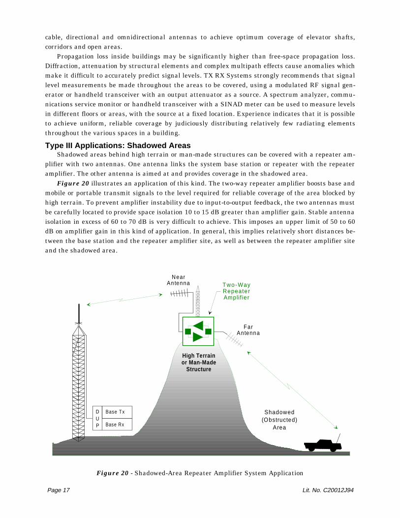
Type III Applications: Shadowed AreasShadowed areas behind high terrain or man-made structures can be covered with a repeater am-

plifier with two antennas. One antenna links the system base station or repeater with the repeateramplifier. The other antenna is aimed at and provides coverage in the shadowed area.

Figure 20 illustrates an application of this kind. The two-way repeater amplifier boosts base andmobile or portable transmit signals to the level required for reliable coverage of the area blocked byhigh terrain. To prevent amplifier instability due to input-to-output feedback, the two antennas mustbe carefully located to provide space isolation 10 to 15 dB greater than amplifier gain. Stable antennaisolation in excess of 60 to 70 dB is very difficult to achieve. This imposes an upper limit of 50 to 60dB on amplifier gain in this kind of application. In general, this implies relatively short distances be-tween the base station and the repeater amplifier site, as well as between the repeater amplifier siteand the shadowed area.

Page 17 Lit. No. C20012J94

NearAn tenna

Base Tx

Base Rx

DUP

Two-WayRepeaterAmplif ier

FarAntenna

High Terrainor Man-Made

Structure

Shadowed(Obstructed)

Area

Figure 20 - Shadowed-Area Repeater Amplifier System Application

Conventional radio repeaters or heterodyne repeater amplifiers that operate on different inputand output frequencies have few limitations on output power and maximum gain. Non-heterodynerepeater amplifiers should be used for shadowed-area applications only when there is no possibility ofoperating on frequencies different from or additional to existing base frequencies.

Real-World ApplicationsReal-world applications usually contain elements of more than one of the above categories. For

example, an airport terminal may have long underground passageways that are treated as tunnels,as well as large open concourses that are best covered with discrete antennas. Underground trans-portation systems typically require communication coverage in train tunnels, passenger platforms,service areas, control and administrative spaces. Optimal designs for such applications involve acombination of different types of signal distribution systems.

Compatible Radio Services All types of radio services can be extended with repeater amplifier systems:

Repeater-based or semiduplex VHF and UHF two-way radioVHF to 900 MHz trunkingVHF or UHF duplex radiotelephoneUHF to GSM cellular radiotelephone (in the U.S., A- and B-band cellular control channelsmust be individually selected and amplified by heterodyne single-channel amplifiers)Telemetry or SCADAPagingData transmission

Stable bidirectional amplification requires that uplink and downlink branch signals be on differ-ent frequencies, to make it possible to provide isolation between branches by means of appropriate fil-ters. The great majority of modern radio applications are two-way duplex or semiduplex, exceptpaging systems, which are one-way. Two-way simplex systems can only be handled in very limitedways with repeater amplifiers.

Page 18 Lit. No. C20012J94

PART III - AMPLIFIER NOISE, INTERMODULATIONAND DYNAMIC RANGE

IntroductionThe preceding section provided a general overview of non-heterodyne repeater amplifier systems

and their applications. We now turn our attention to the application of linear amplifier theory to theestimation of repeater amplifier system performance. We will take the theory for granted, as it hasbeen extensively covered in many classical textbooks and technical papers. We will focus, instead, onthe impact of linear amplifier parameters on system power, noise and intermodulation levels.

The concepts, formulas, data and graphs presented here are eminently practical. In fact, we usethem in our daily work.

NOISENoise deserves special attention in repeater amplifier systems, because amplifier noise defines

the system noise floor. A fundamental system design objective is to achieve receiver input signal-to-noise ratios high enough to produce prescribed output signal-to-noise-ratios or bit error rates. Addi-tionally, amplifier output noise levels must comply with U.S. or international spurious radiationstandards. An understanding of noise figure and its application is essential.

Amplifier Noise FigureNon-ideal amplifiers add noise to signals passing through them. The amplifier noise contribution

can be measured as a ratio of input to output signal-to-noise ratio, as follows:

NF (dB) = 10 log [(S/N)I/(S/N)O] [Eq. 1]

where NF is the noise figure and (S/N)I and (S/N)O are the amplifier input and output signal-to-noiseratios.

The noise figure is 0 dB for a noiseless amplifier or lossless passive device, and is always positivefor non-ideal devices. The noise figure of lossy passive devices is numerically equal to device insertionloss. The typical noise figure of linear amplifier stages ranges from 2 dB or less in low-noise stages, toabout 10 dB in power amplifiers.

If the input of a non-ideal amplifier of gain G dB and noise figure NF dB were connected to amatched resistor, amplifier output noise power would be

PNo (dBm) = 10 log (kT) + 10 log (B) + G + NF [Eq. 2]

where k is Boltzmann's constant (1.38 x 10-20 milliwatts/°K), T is the resistor temperature in degreesKelvin and B is the noise bandwidth in Hz. At room temperature (T = 290o K), and over the 30-KHznoise bandwidth that is frequently used for channel noise power measurements,

PNo (dBm) = -174 + 10 log (30,000) + G + NF = -129.2 + G + NF [Eq. 3]

With NF = 6 dB and G = 100 dB, amplifier noise output power would be -23.2 dBm over a 30-KHzbandwidth. Noise output power is the same over the same noise bandwidth in heterodyne and non-heterodyne amplifiers of the same gain and noise figure. The noise power advantage of heterodynerepeater amplifiers arises from the use of narrowband IF filters that sharply reduce system noisebandwidth.

Noise Figure of Cascaded AmplifiersWhen amplifiers are cascaded, noise power rises towards the output as noise from succeeding

stages is injected into the system. Under the assumption that noise powers add non-coherently, thenoise figure NFT of a cascade consisting of two stages of numerical gain A1 and A2 and noise factor N1

Page 19 Lit. No. C20012J94

and N2, is given by Friis' equation:

NFT = 10 log [N1 + (N2 - 1)/A1] [Eq. 4]

where noise factor is N = 10(NF/10) and numerical gain is A = 10(G/10). Repeated application of Equation4 yields the noise figure of a multistage system.

System noise figure is therefore largely determined by first stage noise figure when A1 is largeenough to make (N2-1)/A1 much smaller than N1. For example, if A1 = 100 (G1 = 20 dB); A2 = 10 (G2 =10 dB); N1 = 2 (NF1 = 3 dB); and N2 = 10 (NF2 = 10 dB), equation 4 yields NFT = 3.2 dB, whereas if A1

were reduced to only 3 (G1 = 4.8 dB), the noisefigure of the cascade would become NFT = 7.0dB.

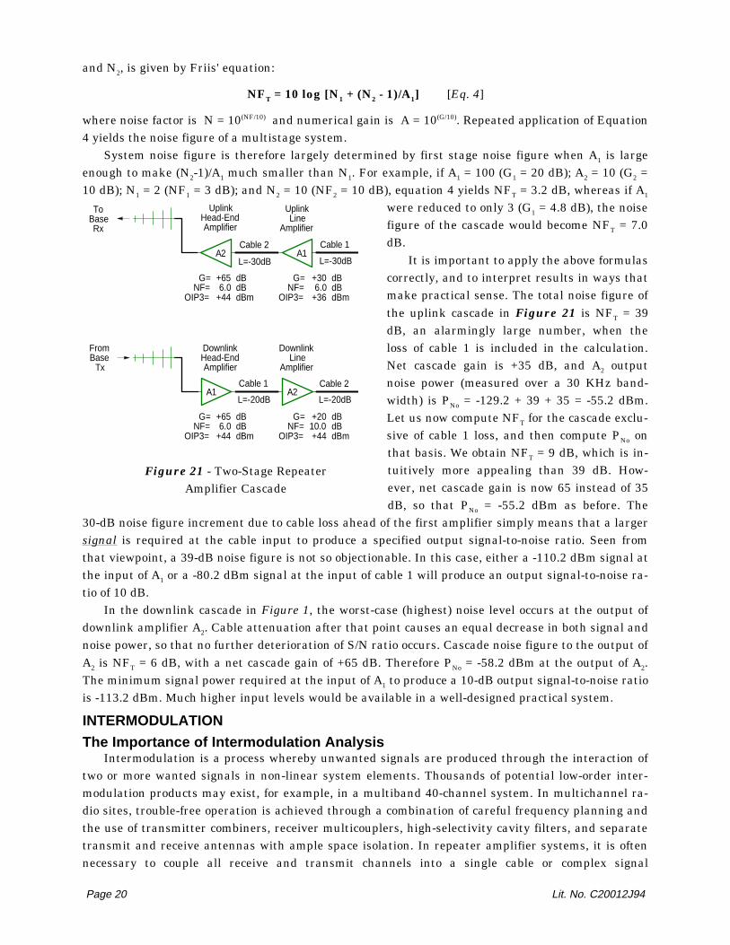
It is important to apply the above formulascorrectly, and to interpret results in ways thatmake practical sense. The total noise figure ofthe uplink cascade in Figure 21 is NFT = 39dB, an alarmingly large number, when theloss of cable 1 is included in the calculation.Net cascade gain is +35 dB, and A2 outputnoise power (measured over a 30 KHz band-width) is PNo = -129.2 + 39 + 35 = -55.2 dBm.Let us now compute NFT for the cascade exclu-sive of cable 1 loss, and then compute PNo onthat basis. We obtain NFT = 9 dB, which is in-tuitively more appealing than 39 dB. How-ever, net cascade gain is now 65 instead of 35dB, so that PNo = -55.2 dBm as before. The

30-dB noise figure increment due to cable loss ahead of the first amplifier simply means that a largersignal is required at the cable input to produce a specified output signal-to-noise ratio. Seen fromthat viewpoint, a 39-dB noise figure is not so objectionable. In this case, either a -110.2 dBm signal atthe input of A1 or a -80.2 dBm signal at the input of cable 1 will produce an output signal-to-noise ra-tio of 10 dB.

In the downlink cascade in Figure 1, the worst-case (highest) noise level occurs at the output ofdownlink amplifier A2. Cable attenuation after that point causes an equal decrease in both signal andnoise power, so that no further deterioration of S/N ratio occurs. Cascade noise figure to the output ofA2 is NFT = 6 dB, with a net cascade gain of +65 dB. Therefore PNo = -58.2 dBm at the output of A2.The minimum signal power required at the input of A1 to produce a 10-dB output signal-to-noise ratiois -113.2 dBm. Much higher input levels would be available in a well-designed practical system.

INTERMODULATION

The Importance of Intermodulation AnalysisIntermodulation is a process whereby unwanted signals are produced through the interaction of

two or more wanted signals in non-linear system elements. Thousands of potential low-order inter-modulation products may exist, for example, in a multiband 40-channel system. In multichannel ra-dio sites, trouble-free operation is achieved through a combination of careful frequency planning andthe use of transmitter combiners, receiver multicouplers, high-selectivity cavity filters, and separatetransmit and receive antennas with ample space isolation. In repeater amplifier systems, it is oftennecessary to couple all receive and transmit channels into a single cable or complex signal

Page 20 Lit. No. C20012J94

To Base

Rx

FromBase

Tx

DownlinkHead-EndAmplifier

UplinkHead-EndAmplifier

UplinkLine

Amplifier

DownlinkLine

Amplifier

G=NF=

OIP3=

dBdBdBm

+656.0

+44

G=NF=

OIP3=

dBdBdBm

+2010.0+44

L=-30dB L=-30dB

L=-20dB L=-20dB

G=NF=

OIP3=

dBdBdBm

+656.0

+44

G=NF=

OIP3=

dBdBdBm

+306.0

+36

A1A2

A1 A2

Cable 1Cable 2

Cable 2Cable 1

Figure 21 - Two-Stage RepeaterAmplifier Cascade

distribution network where all transmit and receive channels coexist everywhere. Under those condi-tions, extreme care must be exercised in predicting potential intermodulation problems.

All multichannel repeater amplifier system designs should begin with an exhaustive intermodu-lation analysis. In systems where all signals flow through a single cable with bidirectional amplifiers,it is mandatory to examine all possible intermodulation products on base transmit and receive chan-nels, and the analysis should extend to high intermodulation orders. In low-power systems withseparate downlink and uplink cables and one-way amplifiers, it is generally sufficient to analyze low-order products on base transmit and receive frequencies.

Two-Carrier Intermodulation and Output Third-Order Intercept PointA non-ideal linear amplifier with two input carriers on frequencies F1 and F2 generates inter-

modulation products on frequencies (mF1±nF2) and (mF2±nF1), where m and n are positive integers.The sum (m+n), an odd integer, defines the order of a product. Third-order intermodulation productson frequencies (2F1±F2) and (2F2±F1) have the largest magnitude and are the basis for worst-caseanalyses. Higher-order products, especially those on frequencies near system receive channels, mustbe considered in systems where multiple repeaters or base station transceivers are connected to sig-nal distribution networks.

When the two carrier frequencies are in the same range, products of the form (2F1+F2) and(2F2+F1) fall completely outside the amplifier passband, on frequencies near the third harmonic of thecarriers. Those products may not need to be considered in single-band systems. In multiband sys-tems, they may interfere with radio equipment operating in another band. For example, third-orderproducts of two transmitters operating on 150.600 and 150.900 MHz would interfere with receiversoperating on 452.100 and 452.4 MHz. If the transmitters had a 1-watt output stage and transmitterintermodulation rejection were -135 dBc, the intermodulation products would appear at a level of-105 dBm, approximately 14 dB above typical receiver sensitivity. This is one of the reasons why theuse of separate downlink and uplink cables is recommended in multiband repeater amplifier systems.

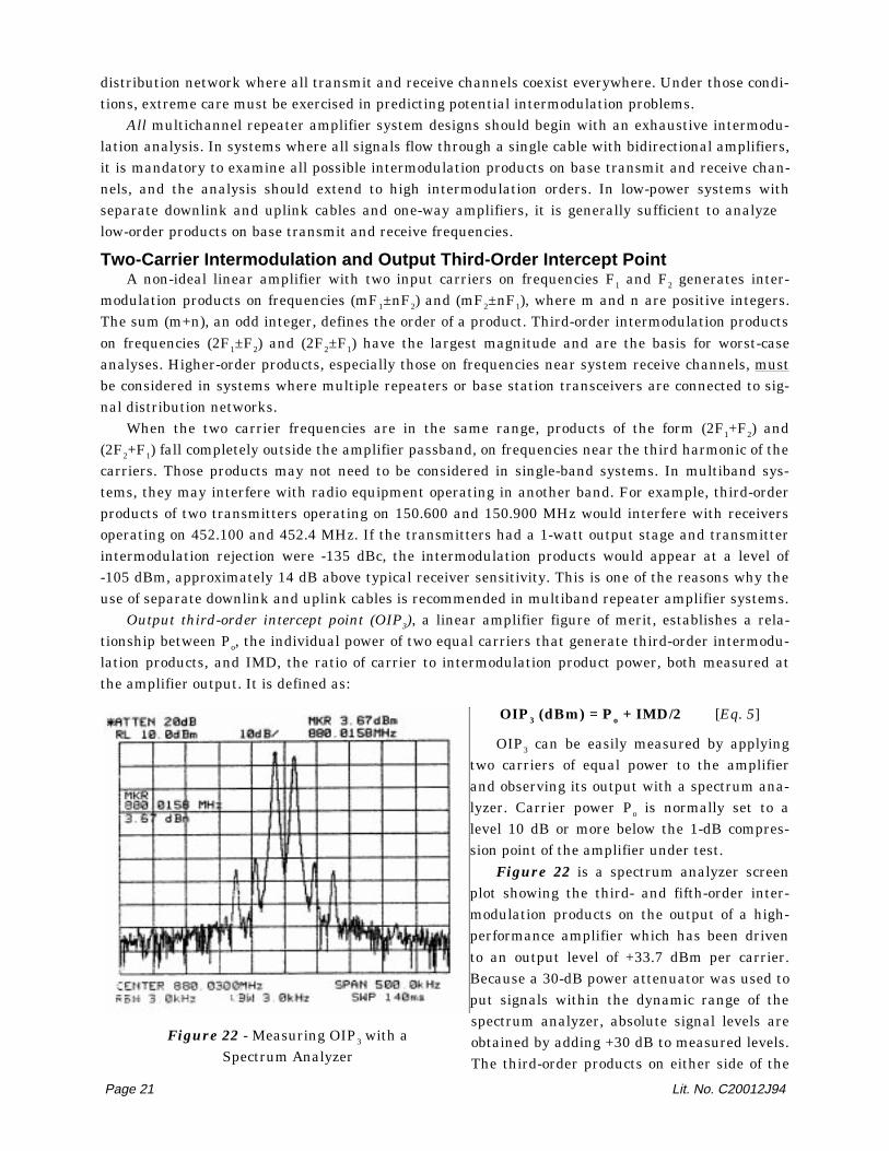
Output third-order intercept point (OIP3), a linear amplifier figure of merit, establishes a rela-tionship between Po, the individual power of two equal carriers that generate third-order intermodu-lation products, and IMD, the ratio of carrier to intermodulation product power, both measured atthe amplifier output. It is defined as:

OIP3 (dBm) = Po + IMD/2 [Eq. 5]

OIP3 can be easily measured by applyingtwo carriers of equal power to the amplifierand observing its output with a spectrum ana-lyzer. Carrier power Po is normally set to alevel 10 dB or more below the 1-dB compres-sion point of the amplifier under test.

Figure 22 is a spectrum analyzer screenplot showing the third- and fifth-order inter-modulation products on the output of a high-performance amplifier which has been drivento an output level of +33.7 dBm per carrier.Because a 30-dB power attenuator was used toput signals within the dynamic range of thespectrum analyzer, absolute signal levels areobtained by adding +30 dB to measured levels.The third-order products on either side of the

Page 21 Lit. No. C20012J94

Figure 22 - Measuring OIP3 with aSpectrum Analyzer

two carriers are 42.5 dB below the carriers. Therefore PO = +33.7 dBm, IMD = 42.5 dB and OIP3 =33.7 + 42.5/2 = +54.9 dBm.

From the above definition of OIP3, a useful equation can be derived for IM3, third-order inter-modulation output power:

IM3 (dBm) = 3Po - 2OIP3 [Eq. 6]

Equation 6 states that there is a 3:1 relationship between third-order intermodulation productpower and carrier power Po . Thus, a 1-dB change in carrier power causes a 3-dB change in inter-modulation product power. Equation 6 also states that there is a 2:1 relationship between output in-tercept point and intermodulation product power. Thus, at a fixed output power, a 1-dB reduction ofintermodulation power requires a 2-dB increase of output intercept point. Output third-order inter-cept point can be increased by using either higher-power amplifiers or amplifiers with feedforward orother intermodulation cancellation techniques. High-power and feedforward linear amplifiers are ex-pensive and require larger, costly power supplies and power backup equipment. Operation at lowercarrier power has tangible cost, reliability and system performance advantages.

The 3:1 relationship between carrier and third-order intermodulation power also holds for inter-modulation caused by any non-linearities in cable joints, connectors, corroded cable clamps, etc. Ra-dio site operators in the U.S. have long known that all systems eventually develop physical flaws thatproduce intermodulation. The repeater amplifier system designer should therefore view with suspi-cion any suggestions to couple high-power transmitters directly into a cable system. High-power sig-nal sources may reduce the number of repeater amplifiers required, but the potential for increasedlong-term trouble is very real. For instance, operating with 100-watt transmitters (Po = +50 dBm) ina cable system with connector or hardware non-linearities will result in third-order intermodulationproducts 39 dB higher than those produced by 5-watt transmitters (Po = +37 dBm), because 3 x(50-37) = 39 dB.

Interestingly enough, when intermodulation problems arise in systems where transmitters andreceivers are directly coupled to a cable, the very first action taken by their operators is to lowertransmitter output power until the problem (hopefully!) disappears. This is not a satisfactory solutionto a problem that can and should be prevented to begin with.

Third-Order Intermodulation Products in Multiple-Carrier SystemsIn a system where N carriers are present on frequencies F1, F2,...,FN, two types of third-order in-

termodulation products need to be considered. Two-carrier products will fall on frequencies given by(2Fi±Fj), where i and j are not equal and vary from 1 to N. Their individual amplitude is given by

IM3(2) (dBm) = 3(P0) - 2(OIP3) [Eq. 7]

Three-carrier products may also occur on frequencies (Fi±Fj±Fk), where i, j and k are not equaland vary from 1 to N. Products of this type are much more numerous than the two-carrier productsdescribed above. They occur at a level approximately 6 dB higher than 2-carrier product levels.Therefore their level can be estimated from

IM3(3) (dBm) = (3Po) - 2(OIP3) + 6 dB [Eq. 8]

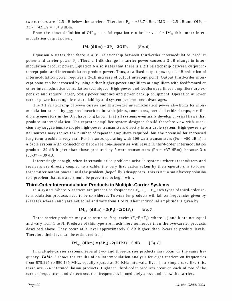
In multiple-carrier systems, several two- and three-carrier products may occur on the same fre-quency. Table 1 shows the results of an intermodulation analysis for eight carriers on frequenciesfrom 879.925 to 880.135 MHz, equally spaced at 30 KHz intervals. Even in a simple case like this,there are 224 intermodulation products. Eighteen third-order products occur on each of two of thecarrier frequencies, and sixteen occur on frequencies immediately above and below the carriers.

Page 22 Lit. No. C20012J94

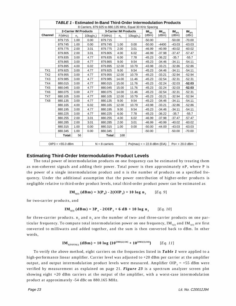
TABLE 1 - Estimated In-Band Third-Order Intermodulation Products8 Carriers, 879.925 to 880.135 MHz, Equal 30 KHz Spacing

Channel2-Carrier IM Products 3-Carrier IM Products IM3(2)

(dBm)IM3(3)

(dBm)IM3(T)

(dBm)IM3(T)

(dBc)F(MHz) n2 10log(n2) F(MHz) n3 10log(n3)879.715 1.00 0.00 879.715 -50.00 -50.00 -70.00 879.745 1.00 0.00 879.745 1.00 0.00 -50.00 -4400 -43.03 -63.03879.775 2.00 3.01 879.775 2.00 3.01 -46.99 -40.99 -40.02 -60.02879.805 2.00 3.01 879.805 4.00 6.02 -46.99 -37.98 -37.47 -57.47879.835 3.00 4.77 879.835 6.00 7.78 -45.23 -36.22 -35.7 -55.7879.865 3.00 4.77 879.865 9.00 9.54 -45.23 -34.46 -34.11 -54.11879.895 4.00 6.02 879.895 12.00 10.79 -43.98 -33.21 -32.86 -52.86

TX1 879.925 3.00 4.77 879.925 9.00 9.54 -45.23 -34.46 -34.11 -54.11TX2 879.955 3.00 4.77 879.955 12.00 10.79 -45.23 -33.21 -32.94 -52.94TX3 879.985 3.00 4.77 879.985 14.00 11.46 -45.23 -32.54 -32.31 -52.31TX4 880.015 3.00 4.77 880.015 15.00 11.76 -45.23 -32.24 -32.03 -52.03TX5 880.045 3.00 4.77 880.045 15.00 11.76 -45.23 -32.24 -32.03 -52.03TX6 880.075 3.00 4.77 880.075 14.00 11.46 -45.23 -32.54 -32.31 -52.31TX7 880.105 3.00 4.77 880.105 12.00 10.79 -45.23 -33.21 -32.94 -52.94TX8 880.135 3.00 4.77 880.135 9.00 9.54 -45.23 -34.46 -34.11 -54.11

880.165 4.00 6.02 880.165 12.00 10.79 -43.98 -33.21 -32.86 -52.86880.195 3.00 4.77 880.195 9.00 9.54 -45.23 -34.46 -34.11 -54.11880.225 3.00 4.77 880.225 6.00 7.78 -45.23 -36.22 -35.7 -55.7880.255 2.00 3.01 880.255 4.00 6.02 -46.99 -37.98 -37.47 -57.47880.285 2.00 3.01 880.285 2.00 3.01 -46.99 -40.99 -40.02 -60.02880.315 1.00 0.00 880.315 1.00 0.00 -50.00 -44.00 -43.03 -63.03880.345 1.00 0.00 880.345 -50.00 -50.00 -70.00

Total: 56 Total : 168

OIP3 = +55.0 dBm N = 8 carriers Po(max) = + 22.8 dBm (EIA) Po= + 20.0 dBm

Estimating Third-Order Intermodulation Product LevelsThe total power of intermodulation products on one frequency can be estimated by treating them

as non-coherent signals and adding their power. Total power is then approximately nP, where P isthe power of a single intermodulation product and n is the number of products on a specified fre-quency. Under the additional assumption that the power contribution of higher-order products isnegligible relative to third-order product levels, total third-order product power can be estimated as

IM3(2) (dBm) = 3(P0) - 2(OIP3) + 10 log n2 [Eq. 9]

for two-carrier products, and

IM3(3) (dBm) = 3Po - 2OIP3 + 6 dB + 10 log n3 [Eq. 10]

for three-carrier products. n2 and n3 are the number of two- and three-carrier products on one par-ticular frequency. To compute total intermodulation power on one frequency, IM3(2) and IM3(3) are firstconverted to milliwatts and added together, and the sum is then converted back to dBm. In otherwords,

IM3(TOTAL) (dBm) = 10 log {10[IM3(2)/10] + 10[IM3(3)/10]} [Eq. 11]

To verify the above method, eight carriers on the frequencies listed in Table 1 were applied to ahigh-performance linear amplifier. Carrier level was adjusted to +20 dBm per carrier at the amplifieroutput, and output intermodulation product levels were measured. Amplifier OIP3 = +55 dBm wereverified by measurement as explained on page 21. Figure 23 is a spectrum analyzer screen plotshowing eight +20 dBm carriers at the output of the amplifier, with a worst-case intermodulationproduct at approximately -54 dBc on 880.165 MHz.

Page 23 Lit. No. C20012J94

The intermodulation analysis indicates that there are four two-carrier and twelve three-carrierproducts at 860.165 MHz. With OIP3 = +55 dBm, Po = +20 dBm, n2 = 4 and n3 = 12, equations 9, 10and 11 predict the following intermodulation levels:

IM3(2) = 3(20) - 2(55) + 10log(4) = -44.0 dBmIM3(3) = 3(20) - 2(55) + 6+ 10log(12) = -33.2 dBmIM3(TOTAL) = 10log{10(-44/10) + 10(-33.2/10)} = 10log(0.00051841) = -32.8 dBmIMD = Po - IM3(TOTAL) = +20 - (-32.8) = 52.8 dBc.

The prediction is therefore slightly on the pessimistic side of the measurements in Figure 23.Even with this high-performance amplifier, operation at +20 dBm per carrier would result in inter-modulation levels not in compliance with the -36 dBm CEPT rule. Compliance would be assured bylowering carrier power by (-36+32.8)/3 = -1.07 dB. +18 dBm per carrier would be a safe operatinglevel.

Equally-spaced carriers cause the worstaccumulation of in-band, third-order inter-modulation products. If conditions permit,unevenly-spaced frequencies should be chosenfor operation with repeater amplifiers.

Intermodulation in CascadedAmplifier Systems

In cascaded amplifier systems, anothercomplication arises from the fact that each am-plifier in the chain sees an input consisting ofwanted signals plus intermodulation productsfrom previous stages. In the worst case, prod-ucts generated in each amplifier add coher-ently with amplified products of previousamplifiers, thereby causing a gradual rise ofintermodulation levels towards the systemoutput.

In systems consisting of cascaded stages of different gain and output intercept point, a practicalway to estimate intermodulation levels is to compute the OIP3 for the entire system, based on theworst-case assumption of coherent addition of intermodulation product power at each stage. In a sys-tem consisting of two cascaded stages of gain G1 and G2 dB, with output intercept points OIP3(1) andOIP3(2) , overall output intercept point OIP3(T) is given by

OIP3(T) (dBm) = -10 log{1/[10[OIP3(1) + G2]/10] + 1/[10OIP3(2)/10]} [Eq. 12]

Repeated application of equation 12 will yield the output intercept point of a multiple-stage sys-tem. Total intermodulation product levels can then be estimated on the basis of OIP3(T) for the ampli-fier chain, with corrections for multiple carriers in accordance with the methods described above.This approach has the advantage of taking into consideration the effect of all system losses, gainsand intercept points.

Consider again the amplifier system in Figure 21 on page 20. Downlink cascade OIP3 is +41dBm, 3 dB less that the OIP3 of the individual stages. In this case, two stages of equal OIP3 operate atthe same output power and contribute equal amounts of intermodulation power at the system output.The underlying assumption in the calculation is that intermodulation powers add in phase, causing a

Page 24 Lit. No. C20012J94

Figure 23 - Eight- Carrier OutputIntermodulation Products

Page 25 Lit No. C2012J94

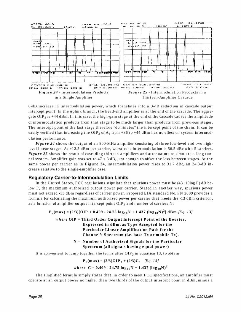
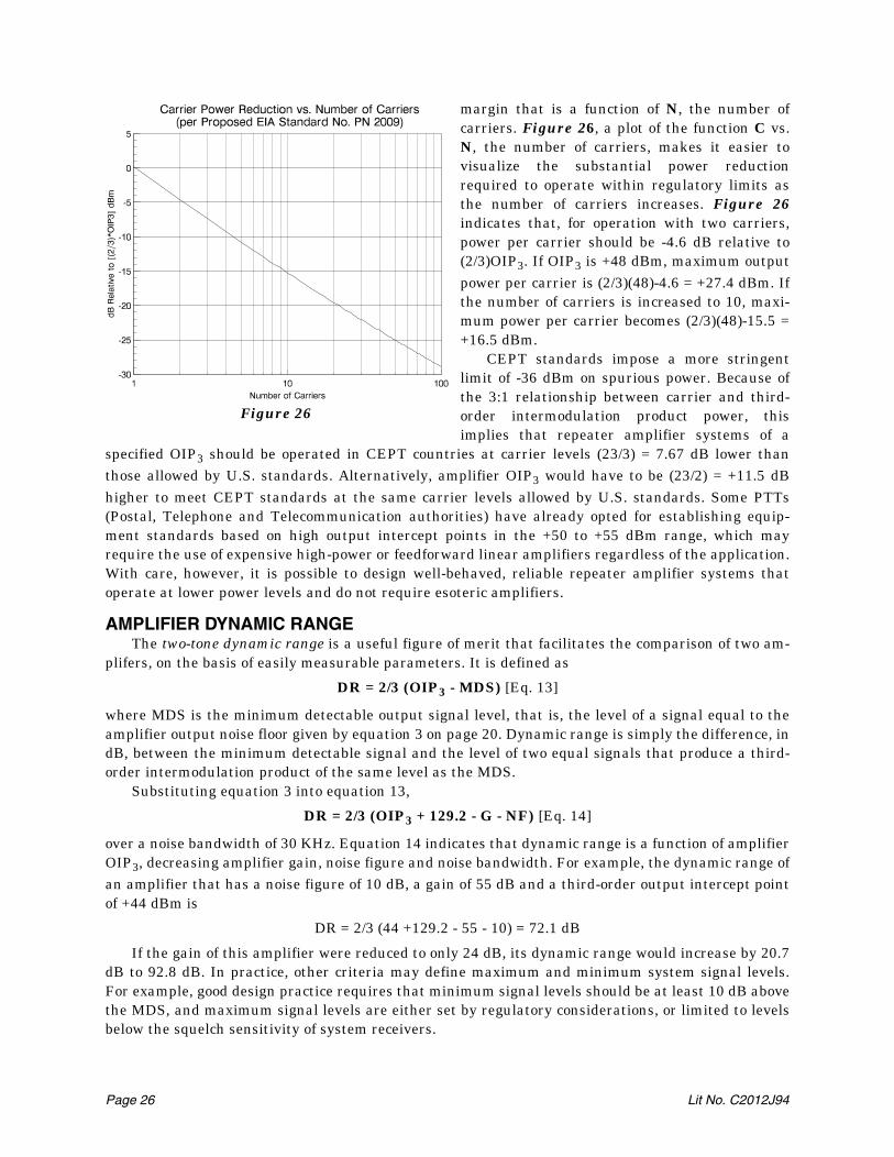
6-dB increase in intermodulation power, which translates into a 3-dB reduction in cascade outputintercept point. In the uplink branch, the head-end amplifier is at the end of the cascade. The aggre-gate OIP3 is +44 dBm. In this case, the high-gain stage at the end of the cascade causes the amplitudeof intermodulation products from that stage to be much larger than products from previ-ous stages.The intercept point of the last stage therefore "dominates" the intercept point of the chain. It can beeasily verified that increasing the OIP3 of A1 from +36 to +44 dBm has no effect on system intermod-ulation performance.

Figure 24 shows the output of an 800-MHz amplifier consisting of three low-level and two high-level linear stages. At +12.5 dBm per carrier, worst-case intermodulation is 56.5 dBc with 5 carriers.Figure 25 shows the result of cascading thirteen amplifiers and attenuators to simulate a long tun-nel system. Amplifier gain was set to 47 ± 3 dB, just enough to offset the loss between stages. At thesame power per carrier as in Figure 24, intermodulation power rises to 31.7 dBc, an 24.8-dB in-crease relative to the single-amplifier case.

Regulatory Carrier-to-Intermodulation LimitsIn the United States, FCC regulations stipulate that spurious power must be (43+10log P) dB be-

low P, the maximum authorized output power per carrier. Stated in another way, spurious powermust not exceed -13 dBm regardless of carrier power. Proposed EIA standard No. PN 2009 provides aformula for calculating the maximum authorized power per carrier that meets the -13 dBm criterion,as a function of amplifier output intercept point OIP3 and number of carriers N:

Pc(max) = (2/3)[OIP + 0.409 - 24.75 log10N + 1.437 (log10N)2] dBm [Eq. 13]

where OIP = Third Order Output Intercept Point of the Booster,Expressed in dBm, as Type Accepted for theParticular Linear Amplification Path for theChannel’s Spectrum (i.e. base Tx or mobile Tx).

N = Number of Authorized Signals for the ParticularSpectrum (all signals having equal power)

It is convenient to lump together the terms after OIP3 in equation 13, to obtain

Pc(max) = (2/3)OIP3 + (2/3)C, [Eq. 14]

where C = 0.409 - 24.75 log10N + 1.437 (log10N)2

The simplified formula simply states that, in order to meet FCC specifications, an amplifier mustoperate at an output power no higher than two thirds of the output intercept point in dBm, minus a

Figure 25 - Intermodulation Products in aThirteen-Amplifier Cascade

Figure 24 - Intermodulation Productsin a Single Amplifier

Page 26 Lit No. C2012J94

margin that is a function of N, the number ofcarriers. Figure 26, a plot of the function C vs.N, the number of carriers, makes it easier tovisualize the substantial power reductionrequired to operate within regulatory limits asthe number of carriers increases. Figure 26indicates that, for operation with two carriers,power per carrier should be -4.6 dB relative to(2/3)OIP3. If OIP3 is +48 dBm, maximum outputpower per carrier is (2/3)(48)-4.6 = +27.4 dBm. Ifthe number of carriers is increased to 10, maxi-mum power per carrier becomes (2/3)(48)-15.5 =+16.5 dBm.

CEPT standards impose a more stringentlimit of -36 dBm on spurious power. Because ofthe 3:1 relationship between carrier and third-order intermodulation product power, thisimplies that repeater amplifier systems of a

specified OIP3 should be operated in CEPT countries at carrier levels (23/3) = 7.67 dB lower thanthose allowed by U.S. standards. Alternatively, amplifier OIP3 would have to be (23/2) = +11.5 dBhigher to meet CEPT standards at the same carrier levels allowed by U.S. standards. Some PTTs(Postal, Telephone and Telecommunication authorities) have already opted for establishing equip-ment standards based on high output intercept points in the +50 to +55 dBm range, which mayrequire the use of expensive high-power or feedforward linear amplifiers regardless of the application.With care, however, it is possible to design well-behaved, reliable repeater amplifier systems thatoperate at lower power levels and do not require esoteric amplifiers.

AMPLIFIER DYNAMIC RANGEThe two-tone dynamic range is a useful figure of merit that facilitates the comparison of two am-

plifers, on the basis of easily measurable parameters. It is defined as

DR = 2/3 (OIP3 - MDS) [Eq. 13]

where MDS is the minimum detectable output signal level, that is, the level of a signal equal to theamplifier output noise floor given by equation 3 on page 20. Dynamic range is simply the difference, indB, between the minimum detectable signal and the level of two equal signals that produce a third-order intermodulation product of the same level as the MDS.

Substituting equation 3 into equation 13,

DR = 2/3 (OIP3 + 129.2 - G - NF) [Eq. 14]

over a noise bandwidth of 30 KHz. Equation 14 indicates that dynamic range is a function of amplifierOIP3, decreasing amplifier gain, noise figure and noise bandwidth. For example, the dynamic range ofan amplifier that has a noise figure of 10 dB, a gain of 55 dB and a third-order output intercept pointof +44 dBm is

DR = 2/3 (44 +129.2 - 55 - 10) = 72.1 dB

If the gain of this amplifier were reduced to only 24 dB, its dynamic range would increase by 20.7dB to 92.8 dB. In practice, other criteria may define maximum and minimum system signal levels.For example, good design practice requires that minimum signal levels should be at least 10 dB abovethe MDS, and maximum signal levels are either set by regulatory considerations, or limited to levelsbelow the squelch sensitivity of system receivers.

Figure 26

PART IV - REPEATER AMPLIFIER SYSTEM ARCHITECTUREThe Repeater Amplifier System Design Process

The primary objective of the repeater amplifier system design process is to provide RF signals toall receivers in the specified coverage area, at levels that satisfy communication reliability, noise andspurious suppression requirements. Simulcast paging, data transmission, spread-spectrum, TDMAand CDMA systems impose additional time-domain requirements, usually expressed in terms of timeand group delay limits within a specified passband. Each repeater amplifier system must be config-ured in accordance with those system design objectives.

As in all radio system engineering work, repeater amplifier system design is an iterative process.It should begin with a complete description of the radio service in which the repeater amplifier sys-tem is intended to operate. As a minimum, the following must be specified:

Type of service (conventional two-way radio, trunking radio, paging, etc.)Nature of the application (mining, government installation, shopping center, etc.)Radio to repeater amplifier system interface (air interface with external base/repeater via antennas, or local radio base station with repeater amplifiers)System frequency plan (individual channel transmit and receive frequencies)Base, mobile and portable radio equipment specifications: transmitter power,receiver sensitivity, receiving and transmitting antenna gain, feedline losses, transmitter combiner loss, receiver multicoupler gain, etc.)If the system operates with a remote base or repeater, measured propagation lossbetween sites and fading margin (a firm system design can only be based onaccurately measured signal levels at key locations)Minimum required signal levels at base, mobile and/or portable receivers

Each of the listed specifications is essential to the design process. Differences between estimatedand actual specifications can be expected to cause significant changes in equipment configuration,performance and price.

A detailed description is also needed of the area in which radio coverage is to be provided by therepeater amplifier system. This should include, as a minimum:

Detailed drawings of the areaThe results of a physical survey indicating how cable can be routed and where equipment and antennas can be installedSystem performance objectives

General statements, such as "the system shall provide a 95% probability of two-way voicecommunication in 95% of the coverage area", or "the bit error rate at 9600 baud shall not be greaterthan 1x10-6 anywhere in the coverage area", should be preferably translated into minimum receiverinput levels at specified worst-case locations. Unrealistic or impractical system design objectivesshould be avoided. Specifications such as "The system shall provide 95% reliability at 95% of the loca-tions, with the user's body in a prone position and completely covering the handheld radio and an-tenna" impose system power and gain requirements beyond the limits of feasibility. Reasonablealternatives should be considered, such as equipping portable radios with a microphone/antenna ac-cessory to be worn at shoulder level.

With those facts on hand, a tentative system design is laid out and preliminary calculations aremade to verify worst-case signal, intermodulation and noise levels. The preliminary analysis usuallyleads to design change recommendations (for example, change one transmitter frequency to eliminatea problematic low-order intermodulation product). Design adjustments are made and the process isrepeated until a design is achieved that satisfies all operating requirements.

Page 27 Lit. No. C20012J94

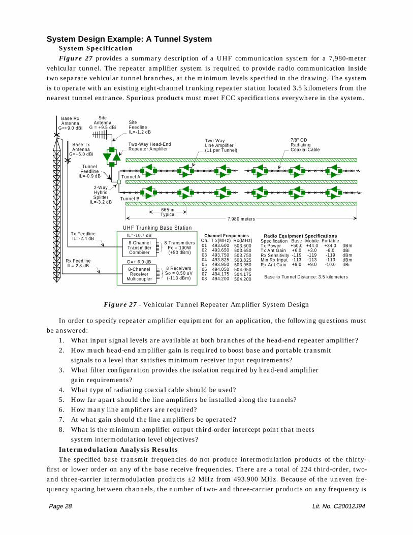
System Design Example: A Tunnel SystemSystem SpecificationFigure 27 provides a summary description of a UHF communication system for a 7,980-meter

vehicular tunnel. The repeater amplifier system is required to provide radio communication insidetwo separate vehicular tunnel branches, at the minimum levels specified in the drawing. The systemis to operate with an existing eight-channel trunking repeater station located 3.5 kilometers from thenearest tunnel entrance. Spurious products must meet FCC specifications everywhere in the system.

In order to specify repeater amplifier equipment for an application, the following questions mustbe answered:

1. What input signal levels are available at both branches of the head-end repeater amplifier?2. How much head-end amplifier gain is required to boost base and portable transmit

signals to a level that satisfies minimum receiver input requirements?3. What filter configuration provides the isolation required by head-end amplifier

gain requirements?4. What type of radiating coaxial cable should be used?5. How far apart should the line amplifiers be installed along the tunnels?6. How many line amplifiers are required?7. At what gain should the line amplifiers be operated?8. What is the minimum amplifier output third-order intercept point that meets

system intermodulation level objectives?Intermodulation Analysis ResultsThe specified base transmit frequencies do not produce intermodulation products of the thirty-

first or lower order on any of the base receive frequencies. There are a total of 224 third-order, two-and three-carrier intermodulation products ±2 MHz from 493.900 MHz. Because of the uneven fre-quency spacing between channels, the number of two- and three-carrier products on any frequency is

Page 28 Lit. No. C20012J94

8-ChannelTransmitterCombiner

8-ChannelReceiver

Multicoupler

8 TransmittersPo = 100W(+50 dBm)

8 ReceiversSo = 0.50 uV(-113 dBm)

IL=-10.7 dB

Two-Way Head-EndRepeater Amplifier

G=+ 6.0 dB

SiteAntenna

G = +9.5 dBi

Base RxAntenna

G=+9.0 dBi

Base TxAntenna

G=+6.0 dBi

2-WayHybridSplitter

IL=-3.2 dB

Tx FeedlineIL=-2.4 dB

Rx FeedlineIL=-2.8 dB

Tunnel A

Tunnel B

Two-WayLine Amplifier(11 per Tunnel)

7/8" ODRadiatingCoaxial Cable

7,980 meters

665 mTypical

SiteFeedlineIL=-1.2 dB

UHF Trunking Base Station

TunnelFeedline

IL=-0.9 dB

SpecificationTx PowerTx Ant GainRx SensitivityMin Rx InputRx Ant Gain

Base+50.0+6.0-119 -113+9.0

Mobile+44.0+3.0-119-113+9.0

Portable+34.0-6.0-119-113-10.0

dBmdBidBmdBmdBi

Channel FrequenciesCh. T x(MHz) Rx(MHz)0102030405060708

493.600493.650493.750493.825493.950494.050494.175494.200

503.600503.650503.750503.825503.950504.050504.175504.200

Radio Equipment Specifications

Base to Tunnel Distance: 3.5 kilometers

Figure 27 - Vehicular Tunnel Repeater Amplifier System Design

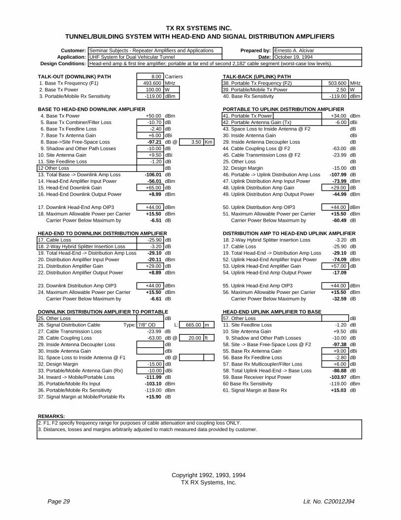
Page 29 Lit. No. C20012J94

TX RX SYSTEMS INC. TUNNEL/BUILDING SYSTEM WITH HEAD-END AND SIGNAL DISTRIBUTION AMPLIFIERS

Customer: Seminar Subjects - Repeater Amplifiers and Applications Prepared by: Ernesto A. AlcivarApplication: UHF System for Dual Vehicular Tunnel Date: October 19, 1994

Design Conditions: Head-end amp & first line amplifier; portable at far end of second 2,182' cable segment (worst-case low levels).

TALK-OUT (DOWNLINK) PATH 8.00 Carriers TALK-BACK (UPLINK) PATH 1. Base Tx Frequency (F1) 493.600 MHz 38. Portable Tx Frequency (F2) 503.600 MHz 2. Base Tx Power 100.00 W 39. Portable/Mobile Tx Power 2.50 W 3. Portable/Mobile Rx Sensitivity -119.00 dBm 40. Base Rx Sensitivity -119.00 dBm

BASE TO HEAD-END DOWNLINK AMPLIFIER PORTABLE TO UPLINK DISTRIBUTION AMPLIFIER 4. Base Tx Power +50.00 dBm 41. Portable Tx Power +34.00 dBm 5. Base Tx Combiner/Filter Loss -10.70 dB 42. Portable Antenna Gain (Tx) -6.00 dBi 6. Base Tx Feedline Loss -2.40 dB 43. Space Loss to Inside Antenna @ F2 dB 7. Base Tx Antenna Gain +6.00 dBi 30. Inside Antenna Gain dBi 8. Base->Site Free-Space Loss -97.21 dB @ 3.50 Km 29. Inside Antenna Decoupler Loss dB 9. Shadow and Other Path Losses -10.00 dB 44. Cable Coupling Loss @ F2 -63.00 dB10. Site Antenna Gain +9.50 dBi 45. Cable Transmission Loss @ F2 -23.99 dB11. Site Feedline Loss -1.20 dB 25. Other Loss dB12 Other Loss dB 32. Design Margin -15.00 dB13. Total Base -> Downlink Amp Loss -106.01 dB 46. Portable -> Uplink Distribution Amp Loss -107.99 dB14. Head-End Amplifier Input Power -56.01 dBm 47. Uplink Distribution Amp Input Power -73.99 dBm15. Head-End Downlink Gain +65.00 dB 48. Uplink Distribution Amp Gain +29.00 dB16. Head-End Downlink Output Power +8.99 dBm 49. Uplink Distribution Amp Output Power -44.99 dBm

17. Downlink Head-End Amp OIP3 +44.00 dBm 50. Uplink Distribution Amp OIP3 +44.00 dBm18. Maximum Allowable Power per Carrier +15.50 dBm 51. Maximum Allowable Power per Carrier +15.50 dBm Carrier Power Below Maximum by -6.51 dB Carrier Power Below Maximum by -60.49 dB

HEAD-END TO DOWNLINK DISTRIBUTION AMPLIFIER DISTRIBUTION AMP TO HEAD-END UPLINK AMPLIFIER17. Cable Loss -25.90 dB 18. 2-Way Hybrid Splitter Insertion Loss -3.20 dB18. 2-Way Hybrid Splitter Insertion Loss -3.20 dB 17. Cable Loss -25.90 dB19. Total Head-End -> Distribution Amp Loss -29.10 dB 19. Total Head-End -> Distribution Amp Loss -29.10 dB20. Distribution Amplifier Input Power -20.11 dBm 52. Uplink Head-End Amplifier Input Power -74.09 dBm21. Distribution Amplifier Gain +29.00 dB 53. Uplink Head-End Amplifier Gain +57.00 dB22. Distribution Amplifier Output Power +8.89 dBm 54. Uplink Head-End Amp Output Power -17.09

23. Downlink Distribution Amp OIP3 +44.00 dBm 55. Uplink Head-End Amp OIP3 +44.00 dBm24. Maximum Allowable Power per Carrier +15.50 dBm 56. Maximum Allowable Power per Carrier +15.50 dBm Carrier Power Below Maximum by -6.61 dB Carrier Power Below Maximum by -32.59 dB

DOWNLINK DISTRIBUTION AMPLIFIER TO PORTABLE HEAD-END UPLINK AMPLIFIER TO BASE25. Other Loss dB 57. Other Loss dB26. Signal Distribution Cable Type: 7/8" OD L: 665.00 m 11. Site Feedline Loss -1.20 dB27. Cable Transmission Loss -23.99 dB 10. Site Antenna Gain +9.50 dBi28. Cable Coupling Loss -63.00 dB @ 20.00 ft 9. Shadow and Other Path Losses -10.00 dB29. Inside Antenna Decoupler Loss dB 58. Site -> Base Free-Space Loss @ F2 -97.38 dB30. Inside Antenna Gain dBi 55. Base Rx Antenna Gain +9.00 dBi31. Space Loss to Inside Antenna @ F1 dB @ 56. Base Rx Feedline Loss -2.80 dB32. Design Margin -15.00 dB 57. Base Rx Multicoupler/Filter Loss +6.00 dB33. Portable/Mobile Antenna Gain (Rx) -10.00 dBi 58. Total Uplink Head-End -> Base Loss -86.88 dB34. Inward -> Mobile/Portable Loss -111.99 dB 59. Base Receiver Input Power -103.97 dBm35. Portable/Mobile Rx Input -103.10 dBm 60 Base Rx Sensitivity -119.00 dBm36. Portable/Mobile Rx Sensitivity -119.00 dBm 61. Signal Margin at Base Rx +15.03 dB37. Signal Margin at Mobile/Portable Rx +15.90 dB

REMARKS:2. F1, F2 specify frequency range for purposes of cable attenuation and coupling loss ONLY.3. Distances, losses and margins arbitrarily adjusted to match measured data provided by customer.

Copyright 1992, 1993, 1994TX RX Systems, Inc.

relatively small (3 and 6). The worst-case on-channel intermodulation product accumulation occurson TX5 (493.950 MHz), where 3 three-carrier products appear. The worst-case off-channel accumula-tion occurs on 493.900 MHz, where 3 two-carrier and 4 three-carrier products appear. Intermodula-tion level calculations are based on those worst cases.

System LayoutGood design practice requires that no more than 24 to 30 dB of loss be allowed between repeater

amplifiers on a cable system. This rule of thumb results in low power, intermodulation and noise lev-els. The rule influences the choice of radiating coaxial cable and the number of repeater amplifiersrequired. Small-diameter cable is less expensive, but its higher loss decreases the maximum allow-able length for 24 dB loss, and this in turn requires a larger number of amplifiers. Large-diameterradiating coaxial cable is very expensive, but it allows the use of longer cable segments and reducesthe number of amplifiers. Depending on the price of the specific cable and repeater amplifiers underconsideration, a cable/amplifier cost analysis generally favors the use of more amplifiers withsmaller-diameter cable. Where maximum performance in a concern, as in multichannel systems, theuse of larger diameter cable should be favored.

In this case in particular, 7/8"-diameter cable is an optimal choice for operation in the 493-504MHz frequency range. 665 meters of cable have a longitudinal transmission loss of approximately 24dB. The 7,980-meter tunnel could therefore be covered by twelve 665-meter cable segments andeleven two-way line amplifiers to compensate for cable losses.

Approval of a design recommendation of this kind normally depends on the availability of physi-cal space and electrical power in the tunnels. The need to install repeater amplifiers in cross-passages or equipment rooms makes it necessary to modify cable lengths and losses accordingly.

Head-End and Line Amplifier Gain CalculationPage 29 is a printout of one of TX RX Systems' worksheets for repeater amplifier system design

calculations. It provides a detailed list of estimated signal levels at key points in the system. Line 9on both columns (Shadow and Other Path Losses) has been arbitrarily adjusted to match the meas-ured signal levels reported by the customer. Other parameters are in accordance with the specifica-tions in Figure 27.

The calculation indicates that head-end downlink amplifier gain should be +65 dB to produceworst-case signal margins of +15.9 dB at a portable receiver at the far end of a cable segment. Be-cause of more favorable antenna gain conditions, an uplink amplifier gain of +57 dB produces a simi-lar margin at the base station receiver, with a portable transmitter at the far end of a cable segment.The resulting amplifier output levels would satisfy FCC standards.

Calculations were also made of maximum signal levels under the following conditions:1. Portable 1 meter away from the near end of a cable segment2. Mobile 3.3 meters away from near end of a cable segment

Case 2 results in maximum uplink amplifier levels that are above the limits suggested by EIAPN2009. The use of output level control is therefore indicated in both the uplink and downlinkbranches of the head-end amplifier.

Cascaded Amplifier Performance CalculationsThe downlink amplifier chain consists of the head-end amplifier (G=+65 dB, NF=+8.0 dB,

OIP3=+44 dBm), 12 cable segments and 11 low-gain line amplifiers (NF=8.0 dB, OIP3 = +44.0 dBm).Each cable segment has an insertion loss of -24 dB, except the first, where hybrid splitter and otherlosses increase total loss to -29.1 dB. The gain of each line amplifier is numerically equal to the cableloss preceding it. The uplink chain is the same as the downlink chain, but in reverse order.

The OIP3 of the complete downlink chain +33.2 dBm. If the OLC of the head-end downlink ampli-fier were set to +9.0 dBm, the level required for satisfactory operation with portables in the tunnels,Page 30 Lit. No. C20012J94

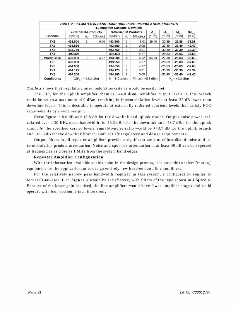
Table 2 shows that regulatory intermodulation criteria would be easily met.The OIP3 for the uplink amplifier chain is +44.0 dBm. Amplifier output levels in this branch

could be set to a maximum of 0 dBm, resulting in intermodulation levels at least 32 dB lower thandownlink levels. This is desirable to operate at externally radiated spurious levels that satisfy FCCrequirements by a wide margin.

Noise figure is 8.0 dB and 18.8 dB for the downlink and uplink chains. Output noise power, cal-culated over a 30-KHz noise bandwidth, is -56.3 dBm for the downlink and -43.7 dBm for the uplinkchain. At the specified carrier levels, signal-to-noise ratio would be +43.7 dB for the uplink branchand +65.3 dB for the downlink branch. Both satisfy regulatory and design requirements.

Output filters in all repeater amplifiers provide a significant amount of broadband noise and in-termodulation product attenuation. Noise and spurious attenuation of at least 40 dB can be expectedat frequencies as close as 1 MHz from the system band edges.

Repeater Amplifier ConfigurationWith the information available at this point in the design process, it is possible to select "catalog"

equipment for the application, or to design entirely new head-end and line amplifiers. For the relatively narrow pass bandwidth required in this system, a configuration similar to

Model 61-68-03-OLC in Figure 5 would be satisfactory, with filters of the type shown in Figure 6.Because of the lower gain required, the line amplifiers would have fewer amplifier stages and couldoperate with four-section, 2-inch filters only.

Page 31 Lit. No. C20012J94

TABLE 2 -ESTIMATED IN-BAND THIRD-ORDER INTERMODULATION PRODUCTS11-Amplifier Cascade, Downlink

Channel2-Carrier IM Products 3-Carrier IM Products IM3(2)

(dBm)IM3(3)

(dBm)IM3(T)

(dBm)IM3(T)

(dBc)F(MHz) n2 10log(n2) F(MHz) n3 10log(n3)

TX1 493.600 1 0.00 493.600 2 3.01 -39.40 -30.39 -29.88 -38.88 TX2 493.650 493.650 1 0.00 -33.40 -33.40 -42.40 TX3 493.750 493.750 2 3.01 -30.39 -30.39 -39.39 TX4 493.825 493.825 3 4.77 -28.63 -28.63 -37.63

Worst Case 493.900 3 4.77 493.900 4 6.02 -34.63 -27.38 -26.63 -35.63 TX5 493.950 493.950 3 4.77 -28.63 -28.63 -37.63 TX6 494.050 494.050 3 4.77 -28.63 -28.63 -37.63 TX7 494.175 494.175 2 3.01 -30.39 -30.39 -39.39 TX8 494.200 494.200 1 0.00 -33.40 -33.40 -42.40

Conditions: OIP3 = + 33.2 dBm N = 8 Carriers P(max)=+8.3 dBm PO = +9.0 dBm

REFERENCES1. "EIA Standard PN 2009 - Proposed Minimum Regulatory Requirements for Cellular Boost-

ers." Electronic Industries Association, Engineering Department, Committee Correspondence,July 31, 1987.

2. "IEEE Standard Definitions of Terms for Radio Wave Propagation". The Institute of Electri-cal and Electronic Engineers, Inc. August 19, 1977.

3. Arandjian, N.: "Simple Computation of Spurious-Free Dynamic Range." RF Design Magazine,January 1987.

4. Bowick, C.: RF Circuit Design. Howard Sams & Co. Inc., Indianapolis, Indiana 1982.5. Burt, D.: "Wireless Communications and the France - U.K. Underwater Tunnel"". Communi-

cations Magazine, May 1991.6. Chadwick, P.E.: "Intermodulation, Phase Noise and Dynamic Range". Presented at the RF

Technology Expo, Anaheim, California 1986.7. Coperich, F. and Turner, C. F.: "FCC Requirements for Type Accepting Radio Signal Boosters

and Licensing Distributed Antenna Systems". Presented at IEEE Vehicular Technology Con-ference, San Diego, California, May 1982.

8. Daniel, J.: "Introduction to TX RX Systems Signal Boosters - OLC Circuit Types." Applicationnote published by The Jack Daniel Company, 6722 Cambridge, Alta Loma, California, 91701.

9. Daniel, J.: "Introduction to Signal Boosters." Application note published by The Jack DanielCompany, 6722 Cambridge, Alta Loma, California, 91701.

10. Fisher, J.: "Multiple RF Channels, Bi-Directional UHF Amplifiers, One Radiating RF Trans-mission Line - A Unique Combination in an Underground Coal Mine Communication System.

11. Gillette, Marlin: Unpublished high-performance linear amplifier test report. TX RX SystemsInc., June 1994.

12. Grüssi, O. and König, P.: "Radio Links for Highway Tunnels". Bulletin Technique PTT7/1978.

13. Gutsche, M.: "Intermod and Connectors: Silver Plate Beats Nickel". Mobile Radio Technology,March 1992.

14. Hayward, W.H.: Introduction to Radio Frequency Design. Prentice Hall, Inc., EnglewoodCliffs, New Jersey, 1989.

15. Kaegebein, Daniel P.: Unpublished system design documentation on numerous in-building,vehicular and railroad tunnel repeater amplifier systems. TX RX Systems Inc., 1979 to 1994.

16. Krauss, H.L.; Bostian, C.W.; Raab, F.H.: Solid State Radio Engineering, John Wiley & Sons,New York - Chichester- Brisbane - Toronto, 1980.

17. Lafortune, J. F. and Lecours, M.: "Measurement and Modeling of Propagation Losses in aBuilding at 900 MHz." IEEE Transactions on Vehicular Technology, Vol. 39, No. 2, May 1990.

18. Lee, R.: "How Washington, D.C.'s Metro Keeps People on the Move." Radio Resource Maga-zine, November/December 1992.

19. Martin, D.J. and Haining, R. W.: "Leaky Feeder Techniques for Mines and Tunnels". Pre-sented at the IERE International Conference on Land Mobile Radio, The University of Lan-caster, Lancaster, England, September 1979.

20. Morgan, M.A. and Sohner, H.K.: "A Radio Communications System for the English ChannelTunnel". IEEE Vehicular Technology Conference Record, 1989.

21. Pfohl, W.: "California SWATS Interference - Part II." Radio Resource Magazine,November/December 1992.

22. Sagers, R.C.: "Intercept Point and Undesired Responses." IEEE Transactions, 1982.23. Simons, K.A.: "The Decibel Relationships Between Amplifier Distortion Products". Proceed-

ings of the IEEE, July 1970.24. Singer, Edward N.: Land Mobile Radio Systems. Prentice Hall, Inc., Englewood Cliffs, New

Jersey, 1989.25. Ward, T.J. and Henderson, L.L.: "An Effective UHF Radio System for Nuclear Generating

Stations". IEEE Transactions, 1982.

Page 32 Lit. No. C20012J94