Rennes 0810041

Position Estimation in Sensor Networks

Brian D O Anderson

Research School of Information Sciences and Engineering, Australian National University

and

National ICT Australia

(Work with A S Morse, D Goldenberg, T Eren)

Rennes 081004 2

OUTLINE

Aim of Presentation Control and Sensor Networks The sensor network localization problem Rigidity and Global rigidity Computational Complexity of

Localization Conclusions and open problems

Aim of presentation

Rennes 081004 3

AIM OF PRESENTATION

To introduce problems involving control and sensor networks

To explain the problem of position estimation of sensors (sensor network localization)

To introduce tools of rigidity To use tools of rigidity theory to understand the

essence of the sensor localization problem Motivations: printers in a building, underwater

acoustic sensors, sensors in dense foliage, etc

Rennes 081004 4

OUTLINE

Aim of Presentation Control and Sensor Networks The sensor network localization problem Rigidity and Global Rigidity Computational Complexity of Localization Conclusions and open problems

Rennes 081004 5

Sensor Networks A collection of sensors is given, in two or

three dimensions. Warning: the earth is not flat!

Typically, the absolute position of some of the sensors (beacons) is known, eg via GPS

Sensors acquire some other position information, eg reciprocally measure distance to neighbours, ie those within a radius r.

Sensors also measure something else--biotoxins, water pressure, fire temperature, etc

Rennes 081004 6

Control problems and Sensor Networks

Covering a region with sensors each may see 3 or 4 others sensors may fail exact positioning may not be

possible region may have irregular

boundaries and/or interior obstacles

Scanning with moving sensors There may be an evader Evader may destroy sensors Sensors with different capabilities Dynamic network A priori or adaptive strategies?

Management of energy usage Sensing radius depends on

power level

Control architecture for swarm What needs to be sensed to

control a moving swarm (eg birds, fish, UAVs)?

Allow for robustness In warfare, may constrain

architecture to avoid disclosure of position when transmitting

Rennes 081004 7

OUTLINE

Aim of Presentation Control and Sensor Networks The sensor network localization problem Rigidity and Global Rigidity Computational Complexity of Localization Conclusions and open problems

Rennes 081004 8

Sensor Networks

Depicts sensors with sensing radius r

r

Sensor

Rennes 081004 9

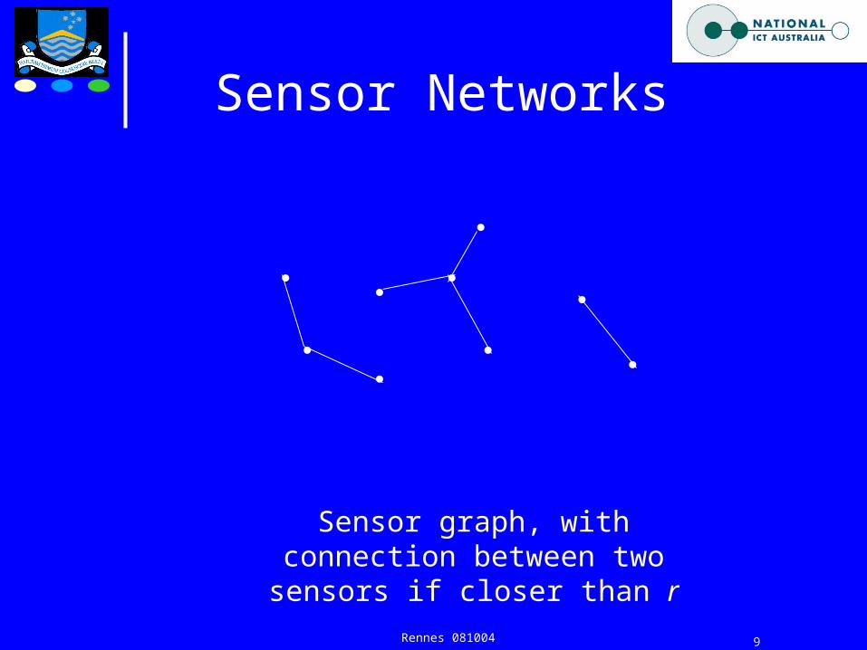
Sensor Networks

Sensor graph, with connection between two sensors if closer than r

Rennes 081004 10

Beacon sensor

Normal sensor

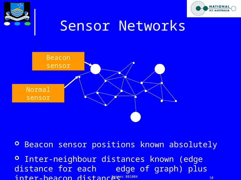
Sensor Networks

Beacon sensor positions known absolutely

Inter-neighbour distances known (edge distance for each edge of graph) plus inter-beacon distances

Rennes 081004 11

Sensor Networks

Beacon sensor positions known absolutely

Inter-neighbour distances known (edge distance for each edge of graph) plus inter-beacon distances

Beacon sensor

Normal sensor

Rennes 081004 12

Sensor Networks-Questions

What are the conditions for network localizability, ie ability to determine the absolute position of all sensors--in first instance from NOISELESS data?

What is the computational complexity of network localization?

The first question is an old one (Cayley, Menger, chemists)

Rennes 081004 13

Sensor Networks-Questions

Need to work with a notion of generic solvability--need solvability for all values of distance round nominal

Could formulate other problems with different inter-sensor information (eg interval of distance values, or direction)

Interest exists in two and three dimensions Not yet studying dynamic networks

Rennes 081004 14

Sensor Networks and Formations

A point formation is a set of points together with a set of links and values for the lengths of the links.

A formation determines a graph G = (V,L) of vertices and edges, and lengths of the edges.

A formation is like a sensor network with the absolute beacon positions thrown away

A formation that is exactly determined by its graph and distance function is globally rigid. Any other formation with the same data is congruent, ie is determinable by translation and/or rotation and/or reflection.

Rennes 081004 15

Congruent Formations

Translation

Reflection

Original position

Absolute beacon positions eliminate this residual uncertainty

Rotation

Rennes 081004 16

Two dimensional rigidity examples

Not rigid--distances do not determine precise

shape.

Globally Rigid--distances determine

shape to within reflection, rotation or

translation

Absolute beacon positions eliminate the reflection etc uncertainty

Rennes 081004 17

Sensor Networks and Formations

Suppose: m beacons, n-m ordinary nodes, for 2 dimensions there are at least 3 beacons in general position, and in 3 dimensions at least 4 beacons in general position.

Then: the sensor localization problem is solvable if and only if the associated formation is globally rigid

Henceforth, we will focus on formations and their global rigidity

Rennes 081004 18

Aim of Presentation Control and Sensor Networks The sensor localization problem Rigidity and Global Rigidity Computational Complexity of

Localization Conclusions and open problems

OUTLINE

Rennes 081004 19

Let F be a formation with vertex and edge sets V and L. Imagine it is moving. Let qi denote the position at time t of the i-th vertex. For each edge (i,j) in L, let (i,j) denote the fixed distance. Then:

(qi - qj) (Dqi - Dqj )= 0 Can write this equation for every edge:

R(F)(Dq) = 0 Here R(F) is the rigidity matrix. For a rigid formation:

1. One rotation and two translations give nullspace of dimension 3 in two dimensions

2. Three rotations and three translations give nullspace of dimension 6 in two dimensions

Rigidity

Rennes 081004 20

Two dimensional rigidity examples

Not rigid. One degree of freedom

“floppiness”. R(F) has 4 dimensional

nullspace

Rigid. R(F) has 3 dimensional nullspace

Rennes 081004 21

Three dimensional rigidity examples

Not rigid. R(F) has 7 dimensional nullspace

Rigid. R(F) has 6 dimensional nullspace

Rennes 081004 22

Rigid Formations

v1 v2 v3 v4

(1,2) x1 - x2 y1 - y2 x1 - x2 y1 - y2 0 0

(1,3) x1 - x2 y1 - y2 0 x1 - x2 y1 - y2 0

(1,4) 0 0 0 x1 - x2 y1 - y2

(2,3) 0 x1 - x2 y1 - y2 x1 - x2 y1 - y2 0

(2,4) 0 x1 - x2 y1 - y2 0 x1 - x2 y1 - y2

(3,4) 0 0 x1 - x2 y1 - y2 x1 - x2 y1 - y2

Sample two dimensional Rigidity Matrix--a Matrix Net ∑ xi Mi +yi Ni in

coordinates xi and yi of points.

Rennes 081004 23

More on rigidity

Rank R(F) for a fixed graph will have the same value for almost all lengths

One has to focus on genericity issues and work with generic rigidity

In two dimensions, there is a combinatorial characterization of generically rigid graphs-Laman’s theorem, with fast algorithm for testing

No such result is available in three dimensions. (Partial results exist)

Rennes 081004 24

Rigidity versus global rigiditya

dc

a

c d

b

b

Both formations are rigid. Neither can be changed into the other by translation, rotation or reflection.They have the same edge

lengths. So they are not globally rigid!

It is possible to have a strictly finite number greater than one of solutions to the formation realization problem --this connotes

rigidity but not global rigidity.

Rennes 081004 25

Rigidity versus global rigidity

We can fix the previous problem if we fix the distance between b and a.

This makes the graph redundantly rigid (and 3-connected, see next slide)

a

c d

b

Rennes 081004 26

Rigidity versus global rigidity Formally, a graph is redundantly rigid if the removal of

any single edge gives a graph that is also generically rigid. A graph is k-connected if the removal of any set of less

than k vertices means that it is still connected. Equivalently, it is k-connected if for any pair of vertices,

one can find k paths joining them, with no common vertices except the end vertices.

Theorem: In two dimensions a graph with at least 4 vertices is generically globally rigid if and only if it is 3-connected and redundantly rigid.

This connects a global property needed to solve estimation problem to a local property holding almost everywhere, for 2D graphs.

Rennes 081004 27

2D Global rigidity--examples Theorem: In two dimensions a graph with at least 4

vertices is generically globally rigid if and only if it is 3-connected and redundantly rigid.

Nontrivial consequence: 6-connectivity is sufficient for global rigidity in two dimensions.

“Wheel” graphs with at least four vertices are globally rigid

Rennes 081004 28

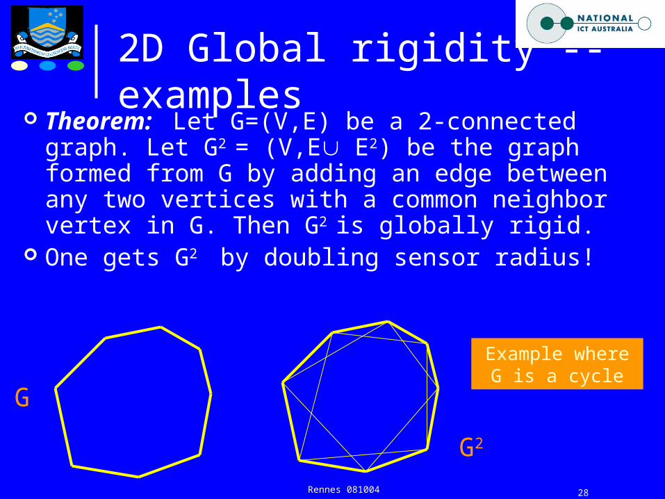
2D Global rigidity --examples Theorem: Let G=(V,E) be a 2-connected

graph. Let G2 = (V,E E2) be the graph formed from G by adding an edge between any two vertices with a common neighbor vertex in G. Then G2 is globally rigid.

One gets G2 by doubling sensor radius!

Example where G is a cycle

G

G2

Rennes 081004 29

3D global rigidity

In three dimensions: If a graph is generically globally rigid, then it is redundantly rigid and at least 4-connected. There is a counterexample to the converse: bipartite graph K5,5

Necessary and sufficient conditions for 3D global rigidity are not known!

In three dimensions, if a particular formation (graph plus distances) is globally rigid, it is not known whether almost all formations with the same graph are globally rigid.

12-connected 3D graphs might be always globally rigid

Rennes 081004 30

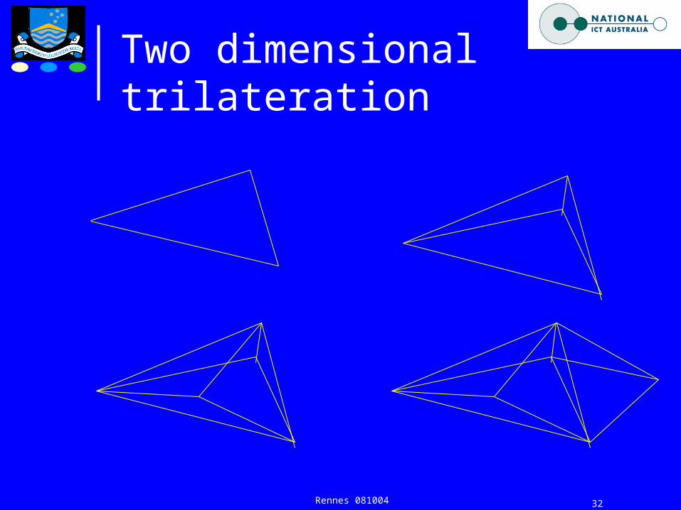
Two dimensional trilateration

Rennes 081004 31

Trilateration One way to construct globally rigid formations: add a

new node to a globally rigid formation, connecting it to d + 1 nodes of the existing formation in general position (d = spatial dimension). Then the new formation is generically globally rigid.

A trilateration graph G in dimension d is one with an ordering of the vertices 1,…d+1,d+2,….n such that the complete graph on the initial d+1 vertices is in G and from every vertex j > d+1, there are at least d+1 edges to vertices earlier in the sequence.

Trilateration graphs are generically globally rigid.

Rennes 081004 32

Two dimensional trilateration

Rennes 081004 33

Nongeneric behaviour

Globally rigid

ab

c

d a

b

cd’

But not globally rigid when a,b,c are collinear!

Globally rigid

Rennes 081004 34

Trilateration Theorem: Let G=(V,E) be a connected graph.

Let G3 = (V,E E2 E3) be the graph formed from G by adding an edge between any two vertices at the ends of a path of 1,2 or 3 edges. Then G3 is a trilateration graph in 2 dimensions.

Also G4 is a trilateration graph in 3 dimensions.

Hence if G(r) is connected, G(3r) is a trilateration in two dimensions, and G(4r) is a

trilateration in three dimensions

Rennes 081004 35

Aim of Presentation Control and Sensor Networks The sensor localization problem Rigidity and Global Rigidity Computational Complexity of

Localization Conclusions and open problems

OUTLINE

Rennes 081004 36

Brute force:

Minimize {(i,j) - || qi - qj ||}2

(i,j) E

Computational Complexity of Localization

Theorem: Trilateration graph is realizable in polynomial time. (Proof relies on finding a seed in polynomial time--choose 3 out of n--and then realizing starting with seed, which is linear time)Theorem: Realization for globally rigid weighted graphs (formations) that are realizable is NP-hard.

(Proof relies on wheel graph and NP-hardness of set-partition -search problem. Heuristic argument on next slide)

Rennes 081004 37

Computational Complexity

Reflection possibilities are linked with computational complexity

Suppose all edge distances known for small triangles.

Localization goes working out from any beacon.

Triangle reflection possibilities grow exponentially….

…and reflection possibilities are only sorted out when one gets to another beacon

Rennes 081004 38

Trilateration localization protocol

Sensors have 2 modes, localized and unlocalized Sensors determine distance from heard transmitter All sensors are pre-placed and listening

Localized mode

Broadcast position

Unlocalized mode

listen for broadcast

IF broadcast from (x,y) heard, determine distance to (x,y)

IF 3 broadcasts heard, determine position and switch to unlocalized mode

Decentralized algorithm!

But how fast?

Rennes 081004 39

Aim of Presentation Control and Sensor Networks The sensor localization problem Rigidity and Global Rigidity Computational Complexity of

Localization Conclusions and open problems

OUTLINE

Rennes 081004 40

Conclusions

Rigidity is not enough; you need global rigidity to localize (+ beacons)

Even then, computational complexity may be terrifying

Polynomial or linear time localization is possible, given trilateration

Change of sensing radius converts connectedness to global rigidity/trilateration

For a class of random sensor graphs, there is not much difference between rigid, globally rigid and trilateration.

Results for 3D are less developed.

Rennes 081004 41

Some Open Problems

Three dimensional graphs Partial localizability Islands of localizability in random graphs Asymmetric sensing radii Angular sensing Measures of ‘health’: graphical, and

geometric Motion of sensors Random graphs.

Rennes 081004 42

Random sensor networks

Sensors may be deployed randomly. We are interested in localization.

The tool is random graph theory (which has been heavily studied)

The random geometric graphs Gn(r) are the graphs associated with two dimensional formations with n vertices with all links of length less than r, where the vertices are points in [0,1]2 generated by a two dimensional Poisson point process of intensity n

Rennes 081004 43

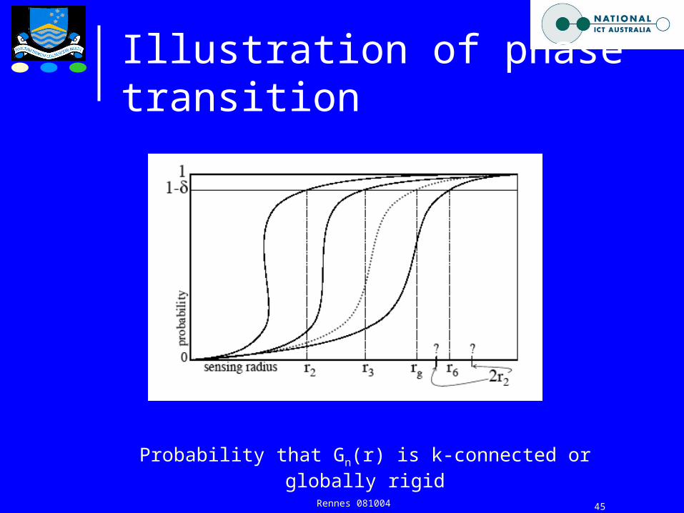
Random geometric graphs

There is a phase transition at which the graph becomes connected with high probability:

r = O(sqrt[(log n)/n]) Connected means: if Gn(r) has a minimum

vertex degree of k then with high probability it is k-connected.

Since 6-connectivity guarantees global rigidity, r = O(sqrt[(log n)/n]) implies global rigidity with high connectivity.

Rennes 081004 44

2D Random geometric graphs If Gn(r) is 2-connected, then Gn(2r) is

globally rigid If Gn(r) is connected, then Gn(3r) is a

trilateration Let r1 ,r2, r3, rg and rt denote the radius at

which Gn(r) is connected, 2-connected, 3-connected, globally rigid and a trilateration with probability 1-. Then for large n,

r6 rg r3 r2

and 3r1 rt 2r2 rg

Rennes 081004 45

Illustration of phase transition

Probability that Gn(r) is k-connected or globally rigid

Rennes 081004 46

Random geometric graphs

All the above have an underlying condition of typer = O(sqrt[(log n)/n])

If nr2/(log n) > 8, then with high probability G is a trilateration graph, and is localizable in linear time given the positions of 3 connected nodes.

Key observation for proof: the density of nodes guarantees one can pick an initial triangle of 3, and then one at a time a new node connected to 3 of those already chosen

It is also localizable in a sort of decentralized fashion.

Rennes 081004 47

Beacons and localization time

Suppose sensors placed with Poisson intensity n and sensing radius r = O(sqrt[(log n)/n]).

If 3 beacons are placed closer than r, can localize in O(sqrt[n/(log n)] steps

If beacons are placed on the unit square by Poisson process with intensity O(n/log n), can localize in O(sqrt(log n)) steps (Key idea: probability that square of side O(r) has 3 beacons is constant p; so some such square has 3 with very high probability)

If beacons are placed by Poisson process of intensity O(n), localization can be effected in O(1) time with very high probability

Rennes 081004 48

Illustration of phase transition

Phase transition is sharper for bigger n

(Beacons all sense one another)

This and next graphs for 3D!

Rennes 081004 49

Theory vs simulation

Sensing radius required to get 95% localization via trilateration

(Beacons all sense one another)

Rennes 081004 50

Speed of localization

Steps required to complete localization vs sensing radius

(Beacons all sense one another)