Embed Size (px)
Citation preview
This file is part of the following reference:
Renagi, Ora (2009) Dispersal patterns and quantities
of sediment discharged from the Markham River, Papua New Guinea. PhD thesis, James Cook
University.
Access to this file is available from:
http://eprints.jcu.edu.au/11679
Dispersal patterns and quantities of sediment
discharged from the Markham River, Papua New
Guinea.
Thesis submitted by
Ora RENAGI (BSc. UPNG, MSc. JCU)
February 2009
for the degree of Doctor of Philosophy in the School of Engineering and Physical Sciences
James Cook University, Townsville, Australia

In Christ Jesus, the Eternal One
To my mother, late Imila Uakai and father, Renagi Puele
My wife Ila and children
Ronald, Lisa Thomas and Jeremiah
2

STATEMENT OF ACCESS
I, the undersigned author of this work, understand that James Cook University will make this thesis available for use within the University Library and, via the Australian Digital Theses network, for use elsewhere. I understand that, as an unpublished work, a thesis has significant protection under the Copyright Act and; I do not wish to place any further restriction on access to this work Or I wish this work to be embargoed until Or I wish the following restrictions to be placed on this work: _____________________________________ ______________ Signature Date

STATEMENT ON SOURCES
Declaration
I declare that this thesis is my own work and has not been submitted in any form for
another degree or diploma at any university or other institution of tertiary education.
Information derived from the published or unpublished work of others has been
acknowledged in the text and a list of references is given.
___________________________ _______________ Signature Date

ELECTRONIC COPY
I, the undersigned, the author of this work, declare that the electronic copy of this thesis provided to the James Cook University Library, is an accurate copy of the print thesis submitted, within the limits of the technology available. _______________________________ _______________ Signature Date

Abstract
The Markham River is a small river draining a tropical mountain range with
altitudes between 1000 to 3000 m. The river has an estimated sediment load of 12
Mtyr-1 and discharges directly into a submarine canyon. The estuary is located
offshore, with a mixing zone outside the river channel. Profiles of salinity and
suspended sediment concentrations (SSC) show that sediment is dispersed via a plume
with components at both the surface, intermediate depth along isopycnal surfaces and
along the steep seabed slopes in the Markham canyon. The dispersal pattern of the
surface freshwater plume is largely determined by the buoyancy force. However
strong northwesterly winds create upwelling along the fringes of the northern coast.
During a high discharge event, the discharge was 1600 kgs-1 which amount to a daily
load of 0.14 Mtons. Estimates of the horizontal sediment flux gradient of the surface
plume along the estuary axis suggested that about 80% of the sediment discharge was
lost to subsurface waters within a radial distance of 2 km from the river mouth. The
layers of sediment within the water column contained about 0.03 Mtons which is
about 30% of the daily discharge. The amount of suspended sediment accumulating in
thick layers over the seabed is estimated to be about 0.4 Mtons which is about 4 times
the daily discharge. Particle fall velocities estimated from the vertical flux indicate
values less than those of highly flocculated material but particles will settle up to 100
m in a day. High SSCs observed near the seabed indicated sediment falling through
the water column into a bottom boundary nepheloid layer. SSCs over the seabed did
not exceed 1000 mgl-1 indicating continuous downslope flow of sediment. Sediment
at this layer was either directly transported from the river mouth or from the seabed
slopes where previously deposited fine material have been resuspended and
transported along the seabed. Some of the sediment is transported by advection to
form layers of high SSC at isopycnal surfaces. SSCs near the seabed of between 250
and 1000 mgl-1 suggest that layers of significantly elevated density existed near the
seabed, moving under the influence of gravity down steep seabed slopes of the
Markham canyon. The SSC data confirms that Markham River is a high yield river
suitable for studying sediment transport mechanisms analogous to systems during low
stand sea levels.
4
The application of the modified hydrodynamic Princeton Ocean Model (POM)
has been successful for the Markham estuary. The model simulates surface plume
distribution patterns under varying discharge and wind conditions which are
comparable with measured data. The model clearly shows the behavior of the surface
plume that tends to mix slowly along the fringes of the coast compared to the mixing
of plume direct to open sea. The effect of the strong northwesterly wind that caused
upwelling, have been well represented by the plume. The model proves to be suitable
for predicting plume behavior for further studies on e.g. influence of changing river
mouth features caused by weather patterns e.g. the El Nino cycle and the effects of the
new tidal basin (700 m x 400 m x 14 m depth) development for the Lae Port Authority
which will be dredged out from the swampy land adjacent to the Milford Haven Bay.
A new instrument called the Triple differential pressure sensor (TDPS) for
measuring small (<100 mgl-1) amounts of depth averaged suspended sediment
concentrations (SSC) has been designed and a prototype built. The new instrument
measures SSC directly without the calibration problems that can be associated with
optical instruments. Although the specification of the differential pressure sensor
indicate that resolutions of up to 10 mgl-1 can be reached, the prototype TDPS had
resolutions of 100 mgl-1. The low resolution can be attributed to the fabrication
process where air pockets may have been trapped within the tubing channels of the
device. Nevertheless, there is potential to improve the sensitivity of the instrument.
The instrument can be used in coastal waters, rivers and lakes.
5

Acknowledgements
I thank my wife, Ila and the children for their total support during my PhD
studies in the past four years.
I acknowledge the Government of Australia for providing the AusAID
scholarship to fund the study program. AusAID has also supported with travel funds
for the field trips.
I am grateful to Professor Peter Ridd for the quality of supervision he has
provided on the project and Dr Heron for his supervision with the numerical model.
I acknowledge the support of Professor Wayne Read and Professor Peter Ridd
for approving funding towards the two field trips. Allowing the use of instruments
provided by James Cook University to collect data is highly appreciated. I thank the
University of Technology for providing additional funding to cover accommodation
and transport costs during the field trips.
Dr Kevin Parnell was kind enough to approve use of equipments purchased
through an ARC LIEF grant no LE0560828. Dr Allan Orpin assisted with reviewing a
paper for publication. I thank Mr Geoff Cavanagh for fabricating parts of the
instrument designed for measuring SSC.
Professor P. Ridd and Dr Stieglitz are sincerely thanked for assisting with
deployment of instruments during the field trip. I acknowledge Geoffrey Billy Feni,
Tauvau Alu, Benson Dekson, Kenny Michael for technical assistance. I am thankful
to Mr Vagi Uakai, Mr John Thomas and Mr Pate Au for providing accommodation
and transport during the field trips.
6
Contents
Abstract ......................................................................................................................... 4
Acknowledgements....................................................................................................... 6
Contents ........................................................................................................................ 7
List of Figures ............................................................................................................. 11
1 Introduction....................................................................................................... 21
1.1 Brief history of sediment transport studies ............................................... 22
1.2 Focus on small rivers in New Guinea ....................................................... 24
1.3 Current Research....................................................................................... 25
1.3.1 TROPICS ................................................................................................. 25
1.3.2 MARGINS Source-to-Sink ...................................................................... 26
1.4 Focus on the Markham River.................................................................... 27
1.4.1 Basin and discharge properties ................................................................ 27
1.4.2 Plume transport effects of industrial developments................................. 28
1.4.3 Plume transport effects on natural ecosystems ........................................ 28
1.5 Hydrodynamic Model of the Lae Harbour................................................ 29
1.6 Instrumentation for measuring small changes in SSC in -situ.................. 29
1.7 Objective of this study .............................................................................. 29
2 Study Area ........................................................................................................ 31
2.1 Markham River ......................................................................................... 31
2.2 The Study Site - The Markham Estuary ................................................... 33
2.3 Regional Tectonics.................................................................................... 33
2.3.1 Geology.................................................................................................... 33
2.3.2 Collision Margin ...................................................................................... 36
2.4 Local weather patterns .............................................................................. 36
2.5 Observed sediment dispersal patterns in the Markham estuary................ 37
2.5.1 Dispersal by surface and subsurface plumes............................................ 38
2.5.2 Changes in river mouth morphology ....................................................... 38
3 Methods............................................................................................................. 40
3.1 Wind, tidal heights and waves .................................................................. 40
3.2 River height and discharge........................................................................ 41
7
3.3 Time series suspended sediment concentration (SSC) ............................. 42
3.4 Current Measurement................................................................................ 42
3.5 Water Column Observations..................................................................... 44
3.6 Sampling for OBS calibrations ................................................................. 44
3.7 Data Processing and Reduction ................................................................ 46
4 Results............................................................................................................... 47
4.1 Time series river height, tidal and wind activity....................................... 47
4.1.1 River Height............................................................................................. 47
4.1.2 River and sediment discharge during the 2006 and 2007 field trips........ 47
4.1.3 The winds................................................................................................. 49
4.1.4 The tidal levels ......................................................................................... 50
4.1.5 Wave activity ........................................................................................... 50
4.2 Time-series SSC data................................................................................ 51
4.3 Current Data.............................................................................................. 54
4.3.1 Current profiles at site 1........................................................................... 54
4.3.2 Drogue Results......................................................................................... 57
4.3.3 Currents and SSC at site 4........................................................................ 58
4.3.4 CTDS profiles in the river and in close proximity outside of the river mouth............................................................................................... 59
4.4 Water Column Observation ...................................................................... 62
4.4.1 CTDS shallow profiles............................................................................. 62
4.4.2 Surface turbidity and salinity distribution................................................ 63
4.5 Deep CTDS Profiles (High Discharge)..................................................... 66
4.5.1 High SSC and mixing at 30-50 m depth on 26/01/06 .............................. 66
4.5.2 Deep profiles showing SSC layers along a isopycnal surface ................. 68
4.5.3 Diverging plumes out of the river mouth................................................. 68
4.5.4 Deep profiles taken in 2007 ..................................................................... 69
4.6 Deep Profiles (Intermediate Discharge).................................................... 73
4.7 Depth profiles showing thermal activity................................................... 75
5 Analysis and Discussion 77
5.1 The river characteristics ............................................................................ 77
5.1.1 The river flow and discharge ................................................................... 77
5.1.2 The bedload transport............................................................................... 78
8
5.2 Estuarine Characteristics........................................................................... 78
5.2.1 Riverine forcing ....................................................................................... 78
5.2.2 Separation of sediment at turbulent mixing zone..................................... 79
5.2.3 Surface Plume Characteristics ................................................................. 80
5.2.3.1 Surface plume flow regime............................................................. 80
5.2.3.2 Degree of Stratification................................................................... 81
5.2.4 Subsurface Water Column Structure........................................................ 81
5.2.4.1 Density structure ............................................................................. 81
5.2.4.2 Layers of sediment over the seabed ................................................ 82
5.3 Variations in Plume SSC .......................................................................... 82
5.3.1 Dispersal by surface plumes .................................................................... 82
5.3.1.1 The high discharge event and its influence..................................... 83
5.3.1.2 The tidal influence .......................................................................... 83
5.3.1.3 The wind influence ......................................................................... 83
5.3.1.4 Upwelling occurring along northern coast...................................... 84
5.4 Sediment budget........................................................................................ 87
5.4.1 Percentages dispersed between surface and subsurface pathways........... 87
5.4.2 Sediment delivery to subsurface waters................................................... 91
5.4.2.1 Mass of sediment layers over isopycnal surfaces. .......................... 91
5.4.2.2 Sediment mass in layers close to the seabed................................... 92
5.5 Summary of dispersal patterns and quantities dispersed .......................... 95
6 Numerical model of the Markham Estuary....................................................... 97
6.1 Introduction............................................................................................... 97
6.2 The POM Model ....................................................................................... 97
6.2.1 Description of the model.......................................................................... 98
6.2.2 Major governing equations ...................................................................... 99
6.3 Application to Markham Estuary............................................................ 100
6.3.1 The model grid system........................................................................... 100
6.3.2 The model parameters and initial conditions ......................................... 102
6.3.3 The boundary conditions........................................................................ 102
6.4 Results of Model ..................................................................................... 103
9
6.4.1 Salinity distributions during northwest winds and changing river discharge ................................................................................................ 103
6.4.2 The surface currents during northwesterly and high discharge ............. 105
6.4.3 Salinity distributions during zero wind and southeast wind .................. 106
6.5 Qualifying the authenticity of the model ................................................ 108
6.5.1 Correlation between model and field salinity data................................. 108
6.5.2 Comparing the model surface plume thickness against measured values ..................................................................................................... 110
6.6 Other applications of the model .............................................................. 112
6.6.1 Results of current patterns predicted for the tidal basin......................... 113
6.6.2 The changing river mouth ...................................................................... 114
6.7 Discussions ............................................................................................. 115
7 Instrumentation for measuring suspended sediment concentration (SSC) .... 118
7.1 Introduction............................................................................................. 118
7.2 The Principle of Design .......................................................................... 119
7.3 Instrument ............................................................................................... 122
7.4 Methods................................................................................................... 124
7.5 Results of sensor voltage output against concentration .......................... 125
7.6 Discussion ............................................................................................... 126
8 Conclusion ...................................................................................................... 128
8.1 Markham estuary .................................................................................... 128
8.2 Sediment dispersal patterns and quantities ............................................. 129
8.3 The hydrodynamic model for the Markham estuary............................... 129
8.4 Triple Differential Pressure Sensor for measuring SSC ......................... 130
References................................................................................................................. 131
Appendix A – Additional Results ............................................................................. 142
Appendix B – Specifications for Differential Pressure Sensor................................. 149
10
List of Figures
Figure 2.1 Map of PNG showing the Markham River. The study area is the
estuary where the Markham River discharges. Other large rivers
on the Island are also shown. ................................................................ 32
Figure 2.2 Google-Earth photo showing the Markham Estuary, the study site.
Lae City port is 1 km away from the river mouth. A mangrove
swamp (known as the Labu Lakes) is in the vicinities of the
Markham River channel. ....................................................................... 34
Figure 2.3 Map of PNG showing the tectonic boundaries along the Ramu-
Markham fault between the Australian plate and the South
Bismark plate. The lower region of the Markham River runs along
the Ramu-Markham fault and discharges into the inner Huon Gulf
(borrowed from Liu et al. (1995)). ........................................................ 35
Figure 2.4 A detailed bathymetry (m) after Buleka et al (1999) showing steep
slopes of the Markham canyon. The average slope is 13o only 30
m away from the mouth. The slopes decrease to 8o about 4 km out
of the river. The northern seabed slopes at 14.9o and there are
regions of 45o slopes at the tectonic plate collision zone at 350 m
water depth. The location of the Butibum River is also shown. .......... 37
Figure 2.5 River mouth features changing with seasonal weather patterns (a)
Google Photo in Jan. 1999, (b) observed in Aug. 2003 (c) of a
Google map captured in Nov. 2003 (d) observed in Jan. 2006 (e)
observed in March 2007........................................................................ 39
Figure 3.1 Map of the study site showing deployment sites (black bold rings
with numbers) for Optical Backscatter (OBS) sensors that
measured time series SSC. Sites E, A and F were initial positions
of drogues that where used for measuring surface and subsurface
(10 m) currents. WS was the site for the weather station that
measured wind speed and direction. ..................................................... 41
Figure 3.2 Enlarged map of the river mouth showing the bathymetry inside
and just outside of the mouth. ............................................................... 43
11
Figure 3.3 Map of study site showing shallow CTDS profiles sites (+) used
for determining surface SSC and salinity distributions and (x with
letters besides) are sites where deep CTDS profiles were taken........... 45
Figure 3.4 Calibration curves for (a) the OBS (n827) and (b) the SSC sensor
for the Falmouth CTDS Profiler. .......................................................... 45
Figure 4.1 Time series Time series of (a) river height, (b) wind direction and
(c) wind speed, (d) tide levels, (e) significant wave height (Hs)
taken during the field trip in 2006. CTDS profiling was carried out
on days indicated by the shaded strips. ................................................. 48
Figure 4.2 Graphs showing (a) the correlation between river discharge and
height. The correlations is used to determine the discharge activity
for Jan. – Feb. 2006 trip (b) for the Mar. 2007 trip (c). CTDS
profiling was carried out on days indicated by the shaded strips.......... 49
Figure 4.3 Graphs showing (a) correlation curve between sediment
discharged and river height. The correlation is used to determine
sediment discharge during 2006 (b) and 2007 (b) field trips. CTDS
profiling was carried out on days indicated by the shaded strips.......... 50
Figure 4.4 Wave spectrum data for 18:01 hrs burst taken on 18/01/06. (a)
Wave energy spectrum showing two types of waves. (b) The
direction ‘from’ which the waves came. Wave type (I) represent
swells coming from the southerly direction and type (II) represent
waves generated by the local northeasterly sea-breeze......................... 51
Figure 4.5 Time series SSC data at (a) site 1 surface, (b) site 1 near seabed,
(c) site 2 surface (d) site 2 near seabed, (e) site 3 near seabed (f)
site 5 near sea bed (g) site 6 near seabed. (Note differences in the
y-axis scale). Shades indicate days on which CTDS profiles were
taken. ..................................................................................................... 53
Figure 4.6 Time series current taken at site 1 for velocity (a) and direction (b)
for cell 7 (sea surface) about 7.45 meters from the seabed, and
velocity (c) and direction (d) for cell 1 which was 0.45 m from the
seabed.................................................................................................... 55
Figure 4.7 Profiles of 1 m vertical bins at site 1 during low tide taken on
01/02/06 showing current (a) velocity (b) direction. The currents
were coming from east to west with velocities of 0.1 ms-1. Current
12
velocities at the lower 3 m of the water column were less than 0.05
ms-1. The horizontal bars represent errors of velocity taken as the
standard deviation of 5 to 6 different velocity readings for profiles
taken during the single low tide period. ................................................ 56
Figure 4.8 Profiles of current (a) velocity (b) direction taken at site 1 on
01/02/06 during high tide showing currents to the east at the
surface and to the southwest near the bottom. The velocities are
around 0.05ms-1..................................................................................... 56
Figure 4.9 Current profiles at site 1 taken during high tide and a strong north-
westerly wind on 02/02/06 showing (a) velocities and (b) direction
to the west at the surface and to the south a depths below 6 m............. 57
Figure 4.10 Velocity vectors for surface and subsurface (10 m depth) drogues
drifting on 15/02/06 between 1030 and 1130hrs at transect I near
the river mouth, between 1310 and 1340 hrs at transect III,
between 1400 and 1430 hrs at the transect II. The wind changed
direction from northwest to southeast at 1330 hrs. ............................... 58
Figure 4.11 InterOcean S4 current meter (current direction and velocity), SSC
and tidal height at site 4 taken on (a) 31/01/06 (b) 01/02/06 during
rising tides (c) 20/02/06 and (d) 22/02/06 during falling tides. ............ 60
Figure 4.12 Depth profiles of (a) salinity, (b) temperature, (c) SSC taken in the
river showing no upstream flow of seawater and (d) salinity, (e)
temperature and (f) SSC taken 10m seaward off the river mouth
taken on 14/03/07 showing ambient seawater properties below the
discharge point. ..................................................................................... 61
Figure 4.13 Profiles of (a) salinity, (b) temperature and (c) SSC taken 14/03/07
and 40 m away from the river mouth indicating a well mixed layer
between 4 and 16 m water depth. Changes in salinity and
temperature at 17 m depth indicates a surface of a different layer
of water body......................................................................................... 62
Figure 4.14 Shallow CTDS data recorded on 20/01/06 showing (a) near
surface SSC profiles at sites (a) A, (b) B and (c) C. Concurrent (d)
salinity (ppt), (e) temperature (oC) and (f) sigma-t’ (kgm-3) profiles
are also shown. ...................................................................................... 63
13
Figure 4.15 Contours of SSC estimated from profiles (sites indicated by +)
taken on 31/01/06 showing a radial distribution in the estuary. ........... 64
Figure 4.16 Contours of salinity estimated from profiles taken on 31/01/06
showing a distribution with a wide area of plume of salinities
between 12 – 14 ppt extending towards the port area. .......................... 65
Figure 4.17 Contours of surface SSC (mgl-1) estimated from profiles taken at
sites (+) on 08/02/06 showing a distribution with extended area of
SSCs between 200 – 300 mgl-1 near the port area................................. 65
Figure 4.18 Surface salinity (ppt) contours estimated from profiles taken on
08/02/06 showing surface plumes with less than 16 ppt edging
along the shorelines. High salinity (~22 ppt) was observed in the
Milford Haven Bay indicating effects of upwelling.............................. 66
Figure 4.19 Map showing sites G, H, I and J where deep profiles were taken
on 26/01/06............................................................................................ 67
Figure 4.20 SSC profiles taken on 26/01/07 along the nearshore zone of the
northern coast at sites G, H, I and J showing high SSC layers
below 25 m depth. This is a thick layer of SSC transported along
isopycnal surface. The profiler did not reach the seabed. ..................... 67
Figure 4.21 Salinity and temperature profiles taken at site G, H, I and J on
26/01/06 showing stratification above 40 m water depth where the
salinity values are less than 34.5 ppt. .................................................... 68
Figure 4.22 (a) SSC (mgl-1) profiles for sites A, B and C (Fig. 4.14) along the
river axis, (b) concurrent salinity (ppt), temperature (oC) and
sigma-t’ (kgm-3) all recorded on 20/01/06 during a period of high
discharge. The arrows indicate an isopycnal surface where layers
of high SSC (1000 mgl-1) existed.......................................................... 69
Figure 4.23 CTDS profiles taken on 20/01/06 during high discharge period. (a)
SSC Profiles at site D, A and E (site locations in figure 4.19)
representing a section across the river mouth. Note that profiles
reached the seabed and the high SSC near the seabed indicate
accumulation of settling sediment (b) Concurrent salinity (ppt),
temperature (oC) and sigma-t’ (kgm-3) for each site. ............................ 71
14
Figure 4.24 Depth SSC profiles taken in March 2007 at sites C, K, L and M
during (a) intermediate discharge (b) 2 days after a high discharge
event (c) 5 days after the same high discharge...................................... 72
Figure 4.25 SSC profile taken on 30/03/07 at site N (Fig. 4.19) near to the
northern coast at 150 m depth showing near-zero SSC in the water
column indicating that sediment layers with high SSC (Fig. 4.24)
are maintained in the canyon................................................................. 73
Figure 4.26 Profiles of (a) SSC (mgl-1) at site A, B and K along the river axis
showing relatively lower SSC in the water column. (b) Concurrent
salinity (ppt) and temperature (oC), all recorded on 06/02/06
during a period of low discharge showing well-mixed layers at the
surface and between 5 and 10m indicating the halocline and below
20m depths indicating a different water body....................................... 74
Figure 4.27 Deep SSC profile recorded at site C on 23/03/07 during a
intermediate discharge period showing existence of high SSC
layers above the seabed. ........................................................................ 75
Figure 4.28 Depth profiles taken at site F of (a) SSC (b) salinity (c)
temperature and (d) sigma-t’ for the down-cast while (e), (f), (g)
and (h) show respective parameters for the up-cast profiles. This
data indicates a possible thermal event. ................................................ 76
Figure 5.1 Google Earth photo showing standing waves (circled) indicating
an outflow with a densimetric Froude number equal to 1 in the
shallow parts of the river mouth............................................................ 77
Figure 5.2 An along-river section of the mouth showing sediment laden river
water interacting with seawater just off the river mouth. Mixing
occurs between the seawater and the river water interface and lifts
off over the ambient sea water. Sediment and freshwater largely
separate at this point and water with high SSC is formed and
moves downslope. ................................................................................. 80
Figure 5.3 Correlation between wind direction and SSC at site 1 (a) and site 2
(b) showing higher SSC during southeasterly winds compared to
lower SSC during northwesterly winds. Correlations between
northwesterly wind speed and SSC for site 1 (c) and for site 2 (d)
show low SSC during high northwesterly wind speeds compared
15
to high SSC during low wind speeds. This indicates that buoyancy
forces dominated wind stress during weak NW winds forcing the
plume towards the northern coast.......................................................... 84
Figure 5.4 Correlation between wind direction and SSC at site 5 (a) and site 6
(b). SSC was relatively higher during northwesterly winds
compared to SSC during southeasterly winds. Correlations
between northwesterly wind speed and SSC are shown for site 5
(c) and for site 6. These graphs indicate that buoyancy forces were
again dominant during weak NW winds forcing the plume towards
the western coast. .................................................................................. 85
Figure 5.5 A photo showing (arrows towards green water body in the bay) as
remnants of upwelling caused by strong northwesterly winds. The
surface plumes from the river move slowly into the bay as the
wind subsides. ....................................................................................... 86
Figure 5.6 Photo showing clean seawater in the northern coast of the Milford
Haven Bay as a result of upwelling caused by strong northwesterly
winds. The surface plume off the Markham River is parallel to the
north coast and edges towards the coast as the winds subside.
Inset: showing the plan of the camera view .......................................... 86
Figure 5.7 Schematic diagram of the estuary showing changes in vertical flux
and load loss within 2 km distance of the river mouth. Estimates of
suspended sediment fall velocities are also shown. .............................. 89
Figure 5.8 Correlation between surface SSC and salinity. Curve I represents a
conservative mixing curve with no sediment lost from suspension.
The points (x) represents the actual salinity and SSC values
estimated from data recorded on 08/02/06 along the river axis. At
a section of the estuary where the salinity is 22 ppt, approximately
70% of material in the surface plume was lost to the sub-surface
layers. .................................................................................................... 90
Figure 5.9 Contours of SSC in the water column obtained by applying the
Kriging function to SSC profiles taken on 20/01/07 (Fig. 4.22(a))
showing sediment layers with ~ 900 mgl-1 at 75 m water depth........... 92
Figure 5.10 The dashed enclosed trapezium shape is the estimated area over
which the subsurface plume spreads. The area (Area I) is used to
16
determine the quantity of sediment existing over isopycnal
surfaces. Area II is used to estimate mass of sediment accumulated
over the seabed. ..................................................................................... 93
Figure 5.11 Contours of SSC in the water column during an intermediate
discharge on 23/03/07. .......................................................................... 94
Figure 5.12 Contours of SSC of the water column from data collected 2 days
after a high discharge event................................................................... 94
Figure 5.13 Contours of SSC in the water column 5 days after a high discharge
event a clear water above with high SSC layers near the seabed.......... 95
Figure 6.1 Grid points in the harbour. The dark lines in the north and west
indicate the shoreline and the colored lines represent the
bathymetry (m). The boundary adjacent to the river is called the
river-mouth boundary.......................................................................... 102
Figure 6.2 Salinity distribution during the northwest winds and low
freshwater discharge (250 m3s-1) from the Markham River end.
Notice the high salinity region in the Milford Haven Bay and close
to the Lae coastline caused by upwelling when the north-westerly
winds drive the surface plume seaward. The shoreline is
represented by the black lines to the north and the west..................... 104
Figure 6.3 Salinity distribution with northwest wind (10 kmhr-1) and
freshwater intermediate discharge of 520 m3s-1. ................................. 104
Figure 6.4 Salinity chart for northwesterly wind high discharge 1200 m3s-1
showing extension of the surface plumes further seaward.................. 105
Figure 6.5 Surface current patterns concurrent with salinity chart (Fig. 6.4)
for northwesterly winds and high discharge (1200 m3s-1)................... 106
Figure 6.6 Salinity distributions for the surface layer (k = 1) at intermediate
level of discharge, which is approximately 520 m-3s-1. Zero wind
has been applied here. The plume extends further seaward
compared to plumes during periods of low discharge. ....................... 107
Figure 6.7 Salinity distribution of the k = 2 layer which is at depths of
(0.018*total water depth). Zero wind was supplied here. This
distribution shows that the clear seawater of 35 ppt is further up
the river axis indicating that the thickness of the surface plume is
very thin, consistent with field measurements (Fig. 4.14). ................. 108
17
Figure 6.8 Salinity chart for intermediate discharge (520 m3s-1) and
southeasterly wind showing strong mixing in the Milford Haven
Bay. The surface mixed layer moves south even during the
southeasterly winds. ............................................................................ 109
Figure 6.9 Surface currents patterns for southeasterly wind and intermediate
discharge (520 m3s-1)........................................................................... 109
Figure 6.10 Correlation between measured surface salinity on 30/03/07 (Fig.
A6) and model salinity distribution (Fig. 6.8) for southeasterly
wind and intermediate discharge. Conditions of discharge and
wind effects applied to model were similar to actual conditions on
30/03/07............................................................................................... 110
Figure 6.11 Isohalines of the surface plumes prepared from model data plotted
for k layers up to 4 m depth with radial distance from the river
mouth. It can be seen that further than 2000 m from the mouth
boundary, the thickness of the plume is greater than the thickness
of the top model layer. ........................................................................ 111
Figure 6.12 Comparing salinity data with distance from the river mouth (a) for
raw model surface results against measured salinity at sites along
the river axis. The raw data are higher than the measured data. (b)
corrected model surface salinity determined by taking the salinity
at k =1 layer as the average value between k = 1 and 2 and taking
the difference of two values from the average value. ......................... 112
Figure 6.13 The plan area of the tidal basin (700 m x 400 m x 14 m depth).
The area will be dredged to 14 m depth and the waste will be
pumped and dumped at 25 m depth 500 m from the river mouth....... 113
Figure 6.14 Surface current patterns during southeasterly wind (10 kmhr-1) and
intermediate discharge (520 m3s-1) conditions showing currents
directed into the tidal basin. ................................................................ 114
Figure 6.15 Currents at k4 depth (0.071 of water depth) showing subsurface
currents directed out of the tidal basin. ............................................... 115
Figure 6.16 Surface current patterns during northeasterly and intermediate
discharge conditions indicating very low (< 0.05 ms-1) flow in the
tidal basin while currents are directed seaward outside of the
Milford Haven Bay. ............................................................................ 116
18

Figure 7.1 Design of the system with a differential pressure sensor to measure
small changes in pressure as sediment falls in enclosed water
column................................................................................................. 123
Figure 7.2 A linear relationship between the pressure sensor output voltage
and concentration. ............................................................................... 125
Figure 7.3 Graph showing the relationship between the raw logger units the
pressure sensor voltage when in response to increasing mass in the
water column. ...................................................................................... 126
Figure 7.4 Graph showing relationship between raw logger units and
concentration for small increments in concentration. 1 logger unit
is equal 100mgl-1. ................................................................................ 126
Figure A 1 Surface SSC (mgl-1) contours produced from shallow CTDS
profiles taken on 16/02/06. The data for each site (+) profiled was
taken as the average SSC of the top 0.5 m of the profile. ................... 142
Figure A 2 Concurrent surface salinity (ppt) contours produced from shallow
CTDS profiles taken on 16/02/06. The data for each site (+)
profiled was taken as the average salinity of the top 0.5 m of the
profile. ................................................................................................. 143
Figure A 3 SSC surface contours for profiles taken on 14/03/07 during
intermediate discharge......................................................................... 143
Figure A 4 Concurrent salinity contours for profiles taken on 14/03/07 .............. 144
Figure A 5 Surface SSC contours estimated over the harbour with profiles
taken on 30/03/07. ............................................................................... 144
Figure A 6 Concurrent salinity contours for profiles taken on 30/03/07 .............. 145
Figure A 7 Map showing sites for deep profiles which are shown in the rest of
the appendix A. ................................................................................... 145
Figure A 8 Deep SSC profiles taken on 17/01/06 taken at sites O, P, Q, R, S,
T, U, V and W (Fig. A7) showing large subsurface SSC layers
beyond 30 m depths with higher values near the river mouth and
decreases with distance from the river mouth. .................................... 146
Figure A 9 Profiles taken near the river mouth at sites A and D (Fig. 3.3)
along the river axis taken on 30/01/07 during high discharge event
showing high (~ 500 mgl-1) in the water column. ............................... 147
19

Figure A 10 SSC profiles near the river mouth and along the river axis taken on
23/03/07 during intermediate discharge showing low SSC at sites
A and B (Fig. 3.3) closer to the river mouth. However, in deep
waters at site C, there were layers of sediment with high SSC
indicating presence of fluid mud......................................................... 147
Figure A 11 SSC profiles taken at site Y (Fig. A7) on 20/01/06 showing a 20 m
thick fluid mud layer over the seabed. ................................................ 148
20
1 Introduction
The knowledge of the mechanisms which influence sediment dispersal patterns
in both the coastal waters and deep oceans is crucial in understanding the formation of
sediment facies in estuaries and stratigraphy in deep oceans. The temporal and spatial
distribution of sediment facies found in coastal waters may explain the hydrodynamic
forces that control dispersal patterns. This information is useful in addressing
sediment activity in the near-shore coastal regions which can affect ecological
systems and industrial developments. Mechanisms that influence sediment transport
in deep waters, on the other hand, are linked to the seabed stratigraphy from which
records of historical climatic changes and processes that control the evolution of
margins and in particular the formation of hydrocarbon resources can be understood.
The controlling parameters that influence sediment transport in estuaries and
oceans are determined by the size of the catchment basin, the altitude of the mountain
ranges and the amount of land exposure to erosion, climate, precipitation and
discharge. The river and the catchment morphology add to the parameters. The
transport pattern in the ocean is further influenced by the estuarine morphology and
seabed geometry, the discharge properties, particle characteristics and the estuarine
hydrodynamics which are influenced by atmospheric and oceanographic conditions.
Much of the studies on sediment transport have been focused on large rivers
probably because of the notion that only large rivers introduce a significant amount of
sediment to the oceans. Transport processes of large rivers which mostly discharge
into wide and passive continental margins are well established. The importance of
small rivers became apparent when Milliman and Syvitski (1992) realised that
previous attempts to calculate global sediment flux (Holeman, 1968; Milliman and
Meade, 1983) did not adequately include the contribution of small rivers which
number in the thousands. Although small mountainous rivers have small individual
loads, their relatively high yield contributed to their significant sediment input into
oceans (Milliman and Syvitsky, 1992). The tectonic nature and the geomorphology of
the catchment and discharge basin drew a lot of interest in further studying the
processes that control dispersal patterns off small mountainous rivers.
21

In this thesis, a major part of the research is focused on determining dispersal
routes of sediment discharged from the Markham River, a small mountainous river in
the north coast of Papua New Guinea. Quantitative estimates of sediment transported
along these routes will also be determined. The processes that control dispersal
patterns will be discussed and presented in the light of global parameters that
influence sediment dispersal from the heads of the rivers to the deep oceans. As a first
addition to the thesis, a hydrodynamic model of the Markham estuary is set up. The
results of the model are useful in predicting plume behavior and surface current
patterns in the estuary under different atmospheric and oceanographic conditions. A
second addition to the thesis involves the design of a non-optical instrument for
directly measuring suspended sediment concentration (SSC) using a differential
pressure sensor.
1.1 Brief history of sediment transport studies
Numerous studies have been previously conducted to understand processes of
sediment transport from the headwaters of discharging rivers to the seabed of deep
oceans. Initial studies were focused on large rivers like the Mississippi, Columbia and
the Amazon (Barnes et al., 1972; Conomos and Gross, 1972; Milliman et al., 1975;
Scruton, 1956; Scruton and Moore, 1953; Wright and Coleman, 1971) and this was
reasonable considering the notion that only large rivers would contribute a significant
amount of sediment to the oceans. Conceptual models of numerous river systems
provided significant insight to sediment dispersal patterns and controlling physical
parameters (Milliman and Jin, 1985; Nittrouer and Kuehl, 1995; Wright et al., 1990).
Most of these large rivers also discharge onto an environment of wide continental
shelves where very little if any sediment is delivered beyond the continental shelves.
However, a marked difference in the surface sediment mineralogy and the bottom
seabed texture (Geyer et al., 2000; Wheatcroft and Bohgeld, 2000; Wheatcroft et al.,
1997) gave way to focusing study of transport patterns within the entire water column
including the surface plumes over continental shelves.
Advances in water column profiling instrumentation also aided scientist to study
subsurface distribution and processes. Eisma and Kalf (1984) showed that 50% of the
river discharged sediment was lost to the subsurface waters while Wright et al. (1990)
clearly illustrated from studies in the Huanghe River that transport of sediment
22
occurred by a surface and subsurface hyperpycnal component. This type of transport
was already hypothesized by Bates (1953). Densities of 20 – 30 gl-1 were required for
hyperpycnal flow to occur in the Huanghe river (Wright et al., 1990) while Mulder
and Syvitski (1995) suggest an average of 25 – 35 gl-1 from their study of exceptional
discharges of world rivers. This study showed that small to medium sized rivers are
able to generate hyperpycnal flow at their mouth which was attributed to the highly
concentrated sediment discharge from mountainous drainage basins in high rainfall
areas. Many large rivers are not able to generate hyperpycnal flow at their river
mouths because of the high sediment retention rates within their large coastal
floodplains. Hyperpycnal flow has been realised as the main mechanism by which
much of the sediment reaches the deep oceans.
Large rivers usually discharge into passive margins and therefore will provide a
better field of study for transport mechanism on passive margins e.g. Fly and
Amazon. The continental shelves are shallow (~100 m) with gradually sloping seabed.
Sediment delivery is usually through surface plumes also known as hypopycnal flow.
However, fluid mud has been observed on the continental shelf which has migrated
downslope along the sea bed under the influence of gravity. Sternberg (1996) and
colleagues (Wright and Friedrichs, 2006) suggested that fluid mud can be transported
downslope along the continental shelves with the help of surface gravity waves and
tidal current forces. These forces can apply enough stress which exceeds the yield
point of fluid mud body over the seabed and cause the mud to migrate downslope
under the influence of gravity.
Recent studies have shown that transport of sediment across wide margins can
be quite complex and the movement of sediment discharged from the rivers to the
nearshore regions and beyond is accomplished through a variety of transport
mechanisms (Kineke et al., 1996). Of particular significance are the density currents,
also know as hyperpycnal flow, that move large volumes of material across the
margin along the seabed slopes as opposed to hypopycnal (surface plumes) or
isopycnal (plumes at intermediate water depths) flow that are primarily dispersed
offshore by local circulation patterns. Hyperpycnal flows are driven by density
difference and can be generated through major river floods or perhaps more
commonly through a variety of estuarine processes such as circulation and rapid
23
settling which concentrate sediment suspensions off river mouths (Kineke and
Sternberg, 1995).
The process of estimating the contribution of sediment to the global ocean by
small rivers, also lead to the study of the factors that determine the sediment load and
yields. Mulder and Syvitski (1995) showed that the geomorphology and the tectonic
nature of these small rivers and their discharge basins were essential factors in
understanding transport of sediment. Many of these small rivers discharge onto active
margins where continental shelves were narrow or absent and provide an opportunity
to study processes occurring during low stands of sea level. The desire to understand
the links between processes that control transport in the high yield environment and
associated stratigraphy lead to the establishment of study groups focused on the study
of dispersal patterns of small rivers.
1.2 Focus on small rivers in New Guinea
A lot of interest has developed recently to study processes in sedimentation in
the small rivers and their discharge environment in the Indo-Pacific Archipelago and
in particular the rivers in New Guinea. Two of the most popular programs
concentrating studies on rivers in New Guinea are the TROPICS (Brunskill, 2004)
and the MARGINS Source-to-Sink (S2S) programs funded by the National Science
Foundation of USA. These rivers are chosen because of the favorable nature of the
geographical and discharge conditions and the virtually undisturbed environment. The
young rugged mountains, along an active margin setting, are greater than 2000 – 3000
m high and provide potential for high energy run-off. The high rainfall of 2 m/year
enhances erosion of soils increasing sediment in the wash-load with a large supply
signal to the ocean of 20 – 25% from New Guinea along with four other islands in the
area namely Boneo, Sumatra, Philippines and Sulawesi. Exposure of land to erosion
always exists because of the tectonic activities exposing land by landslide. High
precipitation soaks the land and reduces its yield point causing landslides. Human
activities such as land clearance for agriculture, farming and mining activities also add
to land exposure. The rivers in the Indo-Pacific collectively discharge a total of 1700
Mtons annually which is 1.5 times the discharge of the Amazon River (Milliman,
1995). These settings enable the flow of highly energetic outflows scouring the river
beds and increasing the sediment load into adjacent oceans.
24
Small rivers with mountainous catchment basins in this region are also more
responsive to episodic events and those in the tectonically active zones often
discharge directly into narrow active margins allowing some of the sediment
discharged to escape to the deep sea. During high energy discharge events, occurrence
of hyperpycnal flow is more likely and can transport sediment over long distances and
be deposited on sea beds forming stratified sediment layers in deep oceans.
Small rivers in New Guinea also provide opportunity to study sediment delivery
over contrasting margin morphology. The numerous studies carried out on the Fly
River gives knowledge of the processes occurring over passive margins where there is
relatively low tectonic activity taking place. The Sepik on the other hand has similar
drainage and discharge properties to the Fly River but discharges onto an active
margin, a highly seismic region where the edge of the Australian continental plate
collides with the south Bismark plate. The continental shelf of the Sepik River
discharge regime is vary narrow (15 km) and much of the sediment is transported
directly into the Sepik Canyon system (Kineke et al., 2000; Walsh and Nittrouer,
2003). The Markham has a similar morphology to the Sepik system where sediment is
delivered into the Markham Canyon and deposited along the collision boundary of
Australian and the South Bismark tectonic plates.
1.3 Current Research
Continuous research in the region on sediment transport processes and related
fields brought scientists together to form a collaborative research program called
TROPICS, an acronym for Tropical River Ocean Processes in Coastal Settings.
TROPICS research provided the impetus for the MARGINS research program.
1.3.1 TROPICS
TROPICS was set up in June 1993 (Brunskill, 2004) after research scientists
who were carrying out oceanographic and geological studies of the coastal shelf and
delta of the Amazon River wanted an additional example of wet tropical river input to
coastal seas. The Fly River and other rivers in New Guinea provided further
opportunities of research and TROPICS was established with a focus to understand
mechanisms and establish models of coastal ocean trapping, bypassing and cycling of
25
solutes and sediments from wet tropical river catchments of high relief on contrasting
coastal shelves.
The TROPICS group ran data acquisition programs mostly in the Fly and the
Sepik rivers and have published papers on sedimentation processes (Alongi et al.,
1996; Brunskill et al., 1995; Harris et al., 1996; Ilahude et al., 2000; Wolanski et al.,
1998).
1.3.2 MARGINS Source-to-Sink
A major study has been funded by the National Science Foundation of the USA
under the MARGINS Source-to-Sink (S2S) Initiative to develop a quantitative
understanding of margin sediment dispersal systems and associated stratigraphy. The
ability to predict dispersal-system behavior has critical implications for understanding
geochemical cycling (e.g., carbon), ecosystem change (tied to global warming and
sea-level rise), and resource management (e.g., soils, wetlands, groundwater, and
hydrocarbons). The S2S initiative was aimed at studying the processes that control the
rate of sediment and solute production in a dispersal system and how the transport of
sediment through these systems alter the magnitude, grain size, and delivery rate to
sediment sinks. Understanding how variations in sediment production, transport and
accumulation in a dispersal system, is preserved by the stratigraphic records was part
of the focus.
The S2S group organized numerous data acquisition programs in the Fly River
discharge regime in the Gulf of Papua (GOP). The S2S group collaborated with the
TROPICS group and published papers (Kineke and Sternberg, 2000; Kineke et al.,
2000; Kuehl et al., 2000; Walsh and Nittrouer, 2003) on sediment activity both
between the Sepik and the Fly rivers. More recently, after a major data acquisition
program in the Gulf of Papua and the Fly and Strickland Rivers, papers on sediment
transport and depositional processes from the terrestrial regions of the river systems
(Aalto et al., 2008; Day et al., 2008; Swanson et al., 2008) have been published.
Studies on processes controlling sediment delivery in the tidally dominated Fly River
delta and the nearshore marine environment (Crockett et al., 2008; Martin et al., 2008;
Ogston et al., 2008) have also been published.
26
The Markham River discharge basin has been an alternative focus area to the
Fly River for the MARGINS S2S program (MARGINS, 2003). Data acquisition have
not been organized, however this thesis should provide information on dispersal
patterns and quantities of sediment introduced at the discharge point of the Markham
River as an initial basis for further research in the area.
1.4 Focus on the Markham River
The study on the Markham River is focused on taking a quantitative approach to
the sediment dispersal activity from a small mountainous river discharging into an
offshore estuary and directly into a deep sea canyon. This research will also serve as a
conduit of knowledge of surface sediment transport patterns within the offshore
estuary which in this particular environment provides useful information relating to
port services and related industry and also to its effects on natural ecosystems.
1.4.1 Basin and discharge properties
Major rivers in Papua New Guinea (PNG) are categorised as small to medium
rivers and the elevations of the drainage basins range between mountainous (~1000
m) to high mountainous (~ 3000 m) (Mulder and Syvitski, 1995). These rivers include
the Markham, Fly, Sepik, Purari, and Ramu. These rivers have small discharge
compared to the big world rivers however the elevation and high rainfall in the region
produces relatively high sediment yields contributing to increased flux to the oceans.
Together with the Mamberano in West Irian, these rivers introduce an approximate
total of 1.5x10⁹ tons of sediment annually onto the narrow and wide margins of the
northern and southern coasts of New Guinea, respectively. This accounts for 16% of
9x10⁹ tons total annual sediment discharged from the rivers in the Indo-Pacific
Archipelago which is approximately equal to 50% of the worlds total delivered to the
oceans from only 3 % of the land mass (Milliman, 1995).
Among the world rivers, Markham River is categorized as a small to medium
given that the drainage basin is 13000 km2 within mountains ranging between 1000 –
3000 m high. The Markham would be listed between the 200th and 300th biggest world
river by size of drainage basin (Milliman and Syvitsky, 1992). The annual rainfall is
2100 mm in the basin. It delivers sediment directly into a Markham Canyon which has
27
slope of 14o (Buleka et al., 1999) from its head to 200 m depth only with 2 km of the
river mouth.
1.4.2 Plume transport effects of industrial developments
The PNG Ports Ltd has its wharf facilities situated only 1 km from the river
mouth in the Lae harbour. The port experienced very high siltation rates between
1997 and 2002 which were attributed to direct transport of suspended sediment from
the river mouth to the wharf via surface plumes. It is imperative to know the actual
cause of this increase during this period because several factors were given as a cause
of this increase. There were three possible causes. Firstly, the high sediment load
discharged by the river due to increased landslide activity in the Markham drainage
basin; secondly, the change in the position of the river mouth and its flow dimensions
and thirdly, industrial developments along the coastal shores affected current patterns
creating backwater zones suitable for accumulation and settling of sediments in the
wharf area.
Further to that, the Port Authority is currently dredging a new 700 m x 400 m x
14 m tidal basin for the development of a new international wharf. Feasibility studies
carried out by Nedeco Haskoning (Nedeco et al., 1980) have indicated that no major
environmental issues should arise as a result of this new development. This implies
that any impact to the environment should be addressed through affordable remedial
measures which apparently should be readily available. However, it is still imperative
that detailed knowledge of sediment transport patterns in the harbour is necessary for
the industry to manage environmental and engineering issues relating to sediment
activity.
1.4.3 Plume transport effects on natural ecosystems
A large mangrove community, know as the Labu Lakes, is separated from the
Markham River channel by land running parallel to the river. The strip of land
provides a barrier between the river channel and a large mangrove swamp that
provides fishing ground for the local Labu people. Recent increase in discharge levels
is threatening the existence of the land barrier and may redirect the river channel
through the mangrove swamp devastating the mangrove community. Increased
sediment discharge also affects the coastal fishing activity and coral communities
28
along the coastal areas. Leatherback turtles are very common in the area and any
effect on their existence by sediment activity is of interest.
1.5 Hydrodynamic Model of the Lae Harbour
The second part of this thesis involves preparation of a hydrodynamic model of
the Lae Harbour. The numerical model that is used here is a modification of the
original Princeton Ocean Model (POM) (Oey and Ezer, 2008) supplied by the
Princeton University. The POM model has been successfully applied to other
estuaries. The model is able to predict the surface plume behavior and sea surface
current patterns in the harbour under varying oceanographic and atmospheric
conditions.
The model should be able to simulate surface plume dispersal activity during
changes in river discharge and wind patterns. The model results will aid in the
understanding of the physical mechanisms that influence the dispersal of surface
plumes.
1.6 Instrumentation for measuring small changes in SSC in -situ
The final part of this thesis includes the development of a prototype instrument
that is capable of measuring SSC in the water column using an ultra-sensitive
differential pressure sensor. The instrument measures the change in the hydrostatic
pressure in the water column which is directly related to the density and to the mass of
material in the water column. The advantage of direct measurement of water density
is that the calibration problems associated with optical instruments are avoided. The
aim was to develop an instrument that used multiple differencing operations to reduce
common mode errors that are associated with differential pressure sensor
measurements.
1.7 Objective of this study
The objective of this study is to determine dispersal routes and the quantities of
the sediment discharged from the Markham River and transported along these routes.
The quantity of discharge and discharge patterns will be discussed in view of the
global parameters that determine sediment load/yield for world-rivers. The quantity of
29
sediment transported by the surface plumes will present information useful for
industrial developments and ecosystems in the vicinity of the estuary. Processes
controlling dispersal patterns and sediment quantities supplied into the Markham
canyon will be discussed in the light of current studies on transport behavior in deep
sea of active margins and beyond the continental shelves. The hydrodynamic model
will provide further understanding of climatic conditions that influence surface
current patterns and hence sediment transport by surface plumes. The development of
the new instrument should aid the collection of additional data necessary to determine
fall and downslope velocities of settling or transported particles in the water column.
The work in this thesis has been prepared for the following publications;
Renagi O., Ridd P. V. and Stieglitz T. F. (2009) Quantifying sediment discharged
from the Markham River, Papua New Guinea. Continental Shelf Research.
(Accepted)
Renagi O., Heron S. and Ridd P.V. (In preparation) A hydrodynamic model of the
Markham River surface plume. Estuarine, Coastal and Shelf Science.
Renagi, O. and Ridd P.V. (In preparation) A new instrument for measuring suspended
sediment concentrations using a differential pressure sensor. Marine Geology.
30
2 Study Area
2.1 Markham River
The Markham River, situated in the northern coast of Papua New Guinea (PNG)
(Fig. 2.1) is the fourth largest river in PNG but its flow regime has not received the
same scientific attention that has been devoted to the Fly and the Sepik rivers.
Reasons for this include the relatively small size of the river in terms of its sediment
discharge load, and the lack of critical biochemical activity introduced upstream by
mining activities such as occurs on the Fly River. There was however, a major study
on the Markham conducted in 1998 by the Coordinating Committee for Coastal and
Offshore Geoscience Programmes in East and Southeast Asia (CCOP) (Buleka et al.,
1999) to determine the usefulness of geoscientific data to analyse the risks associated
with industrial developments in a geologically hazardous coastal environment in Lae.
Sediment transport and sea-bed processes were only qualitatively discussed in this
study (Prior, 1999). Following the environmental study, the PNG Harbours Limited
funded a study to investigate the cause of the high siltation rates in the Lae wharf area
which reached rates of approximately 0.8 m/yr (ECO-Care, 2002) between 1998 and
2002.
The Markham River drains out the Finnisterre and the Central Ranges with a
catchment area of 13000 km2. The average annual rainfall is 2100 mmyr-1 and the
average discharge is about 460 m3s-1 (Maunsell, 1980). The average annual sediment
yield is 150-160 tons/km2 which amounts to a bedload discharge of 2 Mtyr-1 (Nedeco
et al., 1980). The suspended load has been estimated to be 9-12 Mtyr-1 however this
value was taken during a wet season when the river discharge was around 1600 m3s-1
(ECO-Care, 2002). The large range in the sediment discharge estimate is possibly due
to variations in soil erosion activities in the Markham catchment.
31

Figure 2.1 Map of PNG showing the Markham River. The study area is the estuary where the Markham River discharges. Other large rivers on the Island are also shown.
The relative size of the Markham can be better realised by comparing it to the
heavily studied Fly River, which has a catchment of 76000 km2, a discharge of 3600
m3s-1 and sediment load of 85 Mtyr-1 and about the same rainfall. The discharge
regimes however are markedly different between the two rivers. The Fly discharges
onto the passive margin with a wide continental shelf while the Markham discharges
onto an active margin which is totally without a shelf.
To the west of Lae, the Markham River valley has a comparatively low gradient
in its shallow reach. The high sediment load in the shallow reaches of the river result
in a braided river system all the way to its mouth. The river flows in many channels
between silt and gravel bars (Löffler, 1977). The number of outlets to the sea varies
with time. The Markham valley is infilled with sands and gravels that are derived
from the adjacent mountain ranges. Sometimes thick layers of over 10 m of silt and
clay are found in the coarse-grained deposits, e.g. at the location of Markham Bridge,
10 km upstream from the mouth (Coffey and Hollingsworth, 1969 ).
32
2.2 The Study Site - The Markham Estuary
The Markham estuary (Fig. 2.2) cannot be clearly categorized using
classification methods given by Dyer (1973) and Pritchard (1967). However the
estuary falls into the category of an offshore estuary, i.e. the mixing zone is outside
the channel caused by the direct fresh water outflow to the ocean at the river mouth.
The estuary is micro-tidal with typical tides ranging between 1.1 m during spring tides
and 0.4 m during neap tides. There is a relatively strong influence of ocean waves
interacting with the river outflow, and it is common for standing waves with
significant wave height of ~ 1 m to occur adjacent to the river mouth. Inside the river,
the river-bed depth was maintained at ~ 1.6 m to the edge of river mouth. The seabed
dropped sharply from the edge of the river mouth, reaching depths of 40 m, at only 50
m away from the river mouth.
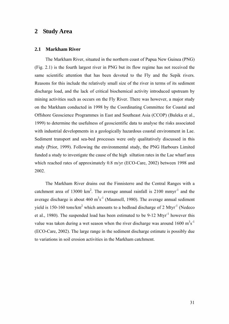
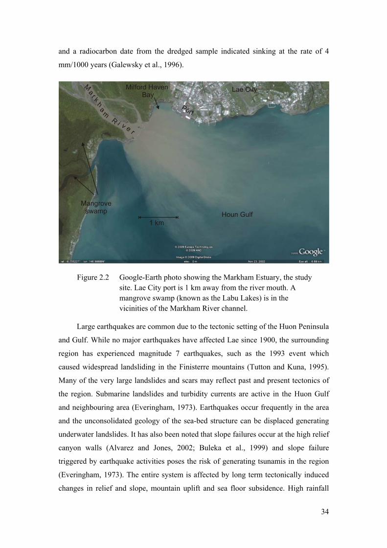
The Lae City is located near the river mouth and the port is situated 1 km from
the river mouth. The port is the main industrial center for transporting goods and
equipment to the highlands and the Islands of northern PNG. Major exports are also
dispatched through the Lae port and any interruptions, e.g. high siltation rates; (ECO-
Care, 2002) to the operations of the port services affects the economy of PNG.
2.3 Regional Tectonics
2.3.1 Geology
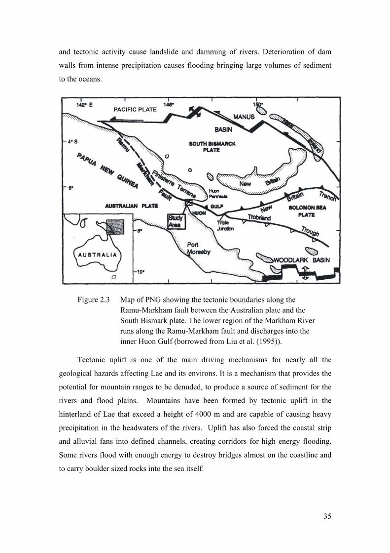
The Markham estuary is located in seismically highly active region, in a
collision margin region between the Australian plate (moving north northeastwards at
about 3 cm/year and the Pacific plate moving west southwest at 7 -10 cm/year. The
South Bismark Plate (Fig. 2.3) is sandwiched between these two major plates giving a
complex pattern of movement. The interactions between the plates produce regional
uplift and subsidence, earthquakes and faults. Lae lies on the northern flank of the
Huon Gulf which is believed to be the location of a major thrust fault known as the
Markham/Ramu lineament. Across the fault there is uplift to the north and subsidence
to the south. On the northern side of the Gulf the 4000 m relief Finisterre mountains,
show uplift rates on the order of 3.5 mm per year, identified from dating of raised
marine terraces ((Chappell, 1974); (Chappell, 1983); (Chappell et al., 1996)). Seismic
reflections over the Huon Gulf have indicated the presence of coral platforms at depth
33
and a radiocarbon date from the dredged sample indicated sinking at the rate of 4
mm/1000 years (Galewsky et al., 1996).
Figure 2.2 Google-Earth photo showing the Markham Estuary, the study site. Lae City port is 1 km away from the river mouth. A mangrove swamp (known as the Labu Lakes) is in the vicinities of the Markham River channel.
Large earthquakes are common due to the tectonic setting of the Huon Peninsula
and Gulf. While no major earthquakes have affected Lae since 1900, the surrounding
region has experienced magnitude 7 earthquakes, such as the 1993 event which
caused widespread landsliding in the Finisterre mountains (Tutton and Kuna, 1995).
Many of the very large landslides and scars may reflect past and present tectonics of
the region. Submarine landslides and turbidity currents are active in the Huon Gulf
and neighbouring area (Everingham, 1973). Earthquakes occur frequently in the area
and the unconsolidated geology of the sea-bed structure can be displaced generating
underwater landslides. It has also been noted that slope failures occur at the high relief
canyon walls (Alvarez and Jones, 2002; Buleka et al., 1999) and slope failure
triggered by earthquake activities poses the risk of generating tsunamis in the region
(Everingham, 1973). The entire system is affected by long term tectonically induced
changes in relief and slope, mountain uplift and sea floor subsidence. High rainfall
34
and tectonic activity cause landslide and damming of rivers. Deterioration of dam
walls from intense precipitation causes flooding bringing large volumes of sediment
to the oceans.
Figure 2.3 Map of PNG showing the tectonic boundaries along the Ramu-Markham fault between the Australian plate and the South Bismark plate. The lower region of the Markham River runs along the Ramu-Markham fault and discharges into the inner Huon Gulf (borrowed from Liu et al. (1995)).
Tectonic uplift is one of the main driving mechanisms for nearly all the
geological hazards affecting Lae and its environs. It is a mechanism that provides the
potential for mountain ranges to be denuded, to produce a source of sediment for the
rivers and flood plains. Mountains have been formed by tectonic uplift in the
hinterland of Lae that exceed a height of 4000 m and are capable of causing heavy
precipitation in the headwaters of the rivers. Uplift has also forced the coastal strip
and alluvial fans into defined channels, creating corridors for high energy flooding.
Some rivers flood with enough energy to destroy bridges almost on the coastline and
to carry boulder sized rocks into the sea itself.
35
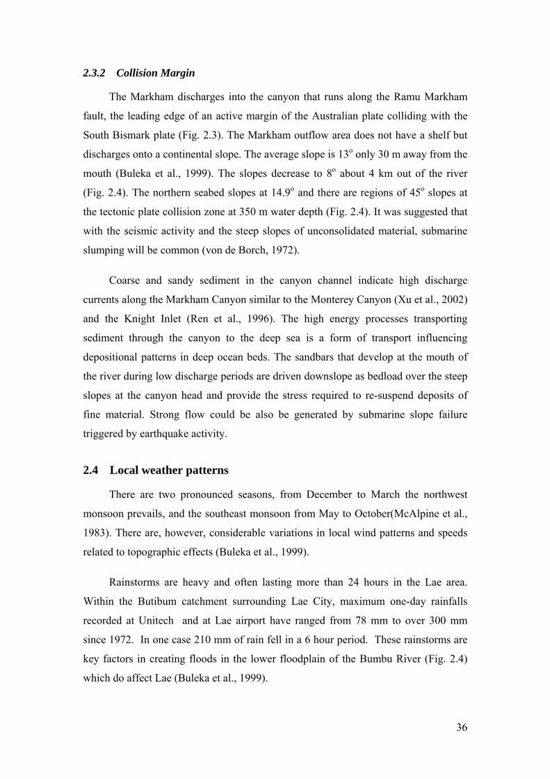
2.3.2 Collision Margin
The Markham discharges into the canyon that runs along the Ramu Markham
fault, the leading edge of an active margin of the Australian plate colliding with the
South Bismark plate (Fig. 2.3). The Markham outflow area does not have a shelf but
discharges onto a continental slope. The average slope is 13o only 30 m away from the
mouth (Buleka et al., 1999). The slopes decrease to 8o about 4 km out of the river
(Fig. 2.4). The northern seabed slopes at 14.9o and there are regions of 45o slopes at
the tectonic plate collision zone at 350 m water depth (Fig. 2.4). It was suggested that
with the seismic activity and the steep slopes of unconsolidated material, submarine
slumping will be common (von de Borch, 1972).
Coarse and sandy sediment in the canyon channel indicate high discharge
currents along the Markham Canyon similar to the Monterey Canyon (Xu et al., 2002)
and the Knight Inlet (Ren et al., 1996). The high energy processes transporting
sediment through the canyon to the deep sea is a form of transport influencing
depositional patterns in deep ocean beds. The sandbars that develop at the mouth of
the river during low discharge periods are driven downslope as bedload over the steep
slopes at the canyon head and provide the stress required to re-suspend deposits of
fine material. Strong flow could be also be generated by submarine slope failure
triggered by earthquake activity.
2.4 Local weather patterns
There are two pronounced seasons, from December to March the northwest
monsoon prevails, and the southeast monsoon from May to October(McAlpine et al.,
1983). There are, however, considerable variations in local wind patterns and speeds
related to topographic effects (Buleka et al., 1999).
Rainstorms are heavy and often lasting more than 24 hours in the Lae area.
Within the Butibum catchment surrounding Lae City, maximum one-day rainfalls
recorded at Unitech and at Lae airport have ranged from 78 mm to over 300 mm
since 1972. In one case 210 mm of rain fell in a 6 hour period. These rainstorms are
key factors in creating floods in the lower floodplain of the Bumbu River (Fig. 2.4)
which do affect Lae (Buleka et al., 1999).
36
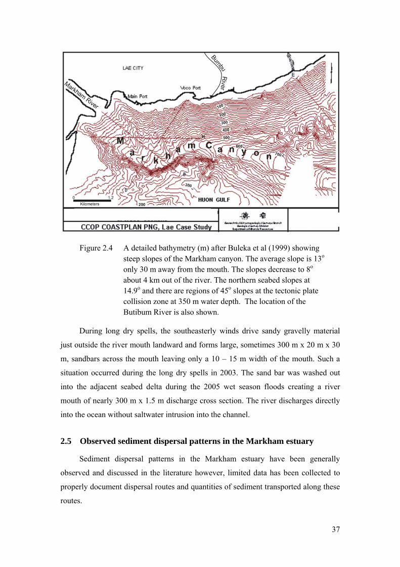
Figure 2.4 A detailed bathymetry (m) after Buleka et al (1999) showing steep slopes of the Markham canyon. The average slope is 13o only 30 m away from the mouth. The slopes decrease to 8o about 4 km out of the river. The northern seabed slopes at 14.9o and there are regions of 45o slopes at the tectonic plate collision zone at 350 m water depth. The location of the Butibum River is also shown.
During long dry spells, the southeasterly winds drive sandy gravelly material
just outside the river mouth landward and forms large, sometimes 300 m x 20 m x 30
m, sandbars across the mouth leaving only a 10 – 15 m width of the mouth. Such a
situation occurred during the long dry spells in 2003. The sand bar was washed out
into the adjacent seabed delta during the 2005 wet season floods creating a river
mouth of nearly 300 m x 1.5 m discharge cross section. The river discharges directly
into the ocean without saltwater intrusion into the channel.
2.5 Observed sediment dispersal patterns in the Markham estuary
Sediment dispersal patterns in the Markham estuary have been generally
observed and discussed in the literature however, limited data has been collected to
properly document dispersal routes and quantities of sediment transported along these
routes.
37
2.5.1 Dispersal by surface and subsurface plumes
Surface plumes are obvious and have been mentioned in some studies (Buleka
et al., 1999; ECO-Care, 2002; Haskoning, 1973). Subsurface plumes however, have
not been measured but inferred from seafloor sediment texture and high relief seabed
features (Krause et al., 1970; Prior, 1999) which indicated occurrence of active high
energy sediment transport processes in the area. Subsurface plumes for the Markham
were inferred by Milliman (1995) using algorithms developed from correlations
between drainage basin area and elevation, rainfall, discharge and suspended sediment
concentration data (Milliman and Syvitsky, 1992). Various studies have suggested
that turbidity currents are active in the area (Liu et al., 1995; Prior, 1999). For
example, movement of large amounts of sediment from the mouth of the Markham
apparently caused damage to SEACOM submarine cables (Krause et al., 1970)
crossing the New Britain trench at water depths of 6000 m. The geometry of the
Markham canyon channel and the distribution of sediment suggest that high density
sediment water mixtures underflow the seawater at the river mouth.
2.5.2 Changes in river mouth morphology
Changes in the morphology of the river mouth can influence dispersal patterns
of sediment in the estuary. These changes were documented using Google Earth
imagery and observations by the author and are shown as sketches in figure 2.5. In
1999, the river mouth was wide open (Fig. 2.5(a)). In August 2003, a large sand bar
(300 m long x 20 m wide x 3 m high from sea level) (Fig. 2.5(b)) was observed across
the mouth of the Markham River. This sandbar was formed after a prolonged dry
season resulting from the El Nino in 2002/03. The river discharge was very low and
waves generated by the southeasterly winds drove back deltaic sand deposits at the
river mouth to form the sandbars. The river mouth was reduced to the extreme
northern end of the river with a 5 – 10 m wide opening. A sketch of the Google Earth
photo taken on 23/11/03 (Fig. 2.5(c)) shows remnants of the sandbar after the wet
season floods washed out parts of the sandbar into the sea. Figure 2.5(d) shows the
river mouth features observed in January 2006. Figure 2.5(e) shows the river features
observed in March 2007.
38
Figure 2.5 River mouth features changing with seasonal weather patterns (a) Google Photo in Jan. 1999, (b) observed in Aug. 2003 (c) of a Google map captured in Nov. 2003 (d) observed in Jan. 2006 (e) observed in March 2007.
39
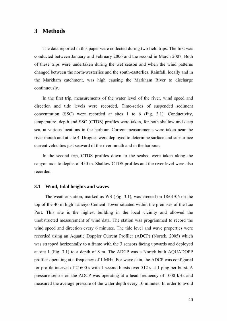
3 Methods
The data reported in this paper were collected during two field trips. The first was
conducted between January and February 2006 and the second in March 2007. Both
of these trips were undertaken during the wet season and when the wind patterns
changed between the north-westerlies and the south-easterlies. Rainfall, locally and in
the Markham catchment, was high causing the Markham River to discharge
continuously.
In the first trip, measurements of the water level of the river, wind speed and
direction and tide levels were recorded. Time-series of suspended sediment
concentration (SSC) were recorded at sites 1 to 6 (Fig. 3.1). Conductivity,
temperature, depth and SSC (CTDS) profiles were taken, for both shallow and deep
sea, at various locations in the harbour. Current measurements were taken near the
river mouth and at site 4. Drogues were deployed to determine surface and subsurface
current velocities just seaward of the river mouth and in the harbour.
In the second trip, CTDS profiles down to the seabed were taken along the
canyon axis to depths of 450 m. Shallow CTDS profiles and the river level were also
recorded.
3.1 Wind, tidal heights and waves
The weather station, marked as WS (Fig. 3.1), was erected on 18/01/06 on the
top of the 40 m high Taheiyo Cement Tower situated within the premises of the Lae
Port. This site is the highest building in the local vicinity and allowed the
unobstructed measurement of wind data. The station was programmed to record the
wind speed and direction every 6 minutes. The tide level and wave properties were
recorded using an Aquatic Doppler Current Profiler (ADCP) (Nortek, 2005) which
was strapped horizontally to a frame with the 3 sensors facing upwards and deployed
at site 1 (Fig. 3.1) to a depth of 8 m. The ADCP was a Nortek built AQUADOPP
profiler operating at a frequency of 1 MHz. For wave data, the ADCP was configured
for profile interval of 21600 s with 1 second bursts over 512 s at 1 ping per burst. A
pressure sensor on the ADCP was operating at a head frequency of 1000 kHz and
measured the average pressure of the water depth every 10 minutes. In order to avoid
40
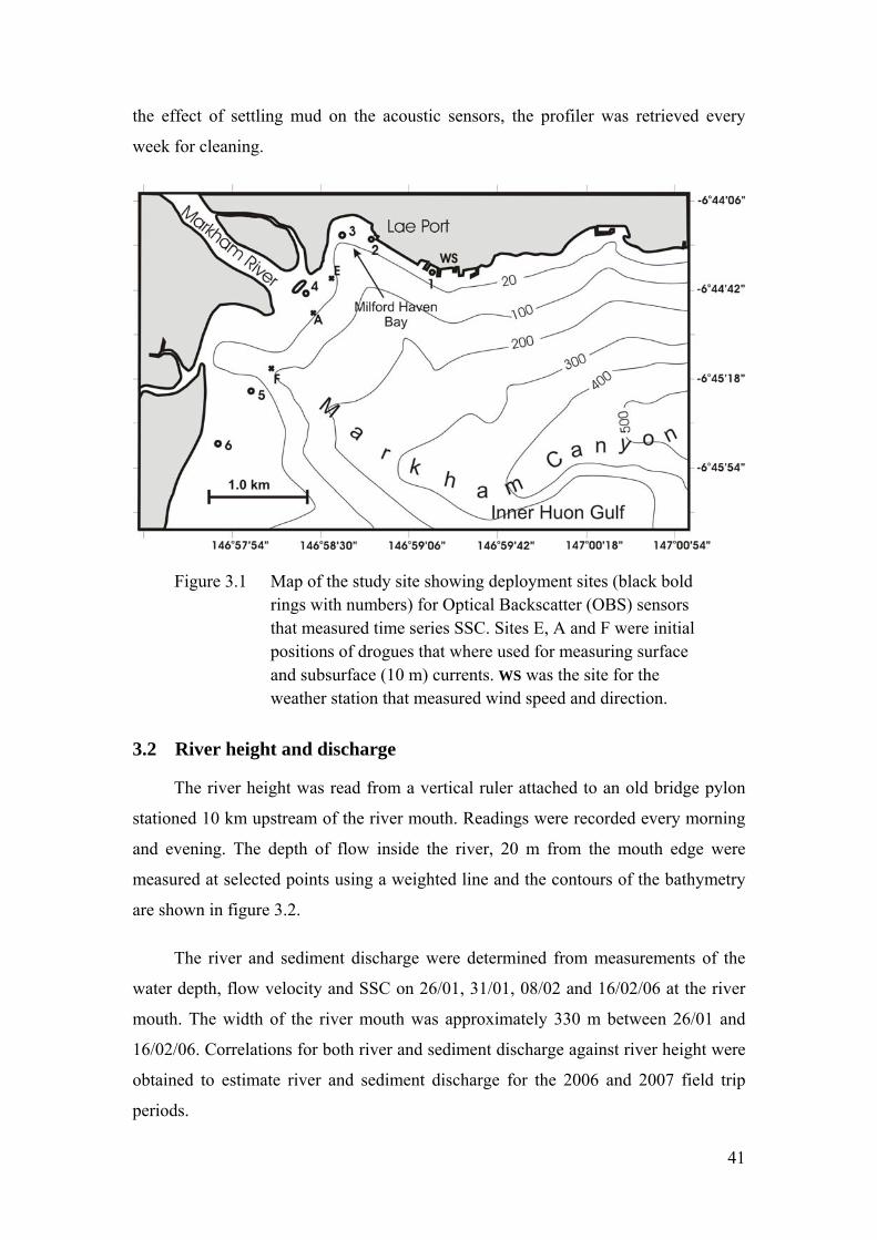
the effect of settling mud on the acoustic sensors, the profiler was retrieved every
week for cleaning.
Figure 3.1 Map of the study site showing deployment sites (black bold rings with numbers) for Optical Backscatter (OBS) sensors that measured time series SSC. Sites E, A and F were initial positions of drogues that where used for measuring surface and subsurface (10 m) currents. WS was the site for the weather station that measured wind speed and direction.
3.2 River height and discharge
The river height was read from a vertical ruler attached to an old bridge pylon
stationed 10 km upstream of the river mouth. Readings were recorded every morning
and evening. The depth of flow inside the river, 20 m from the mouth edge were
measured at selected points using a weighted line and the contours of the bathymetry
are shown in figure 3.2.
The river and sediment discharge were determined from measurements of the
water depth, flow velocity and SSC on 26/01, 31/01, 08/02 and 16/02/06 at the river
mouth. The width of the river mouth was approximately 330 m between 26/01 and
16/02/06. Correlations for both river and sediment discharge against river height were
obtained to estimate river and sediment discharge for the 2006 and 2007 field trip
periods.
41
3.3 Time series suspended sediment concentration (SSC)
Optical Backscatter (OBS) sensors (Ridd and Larcombe, 1994) were each
configured to log SSC data with an interval-time of 10 minutes. The OBS sensor
operates by transmitting infrared light for 20 s (record time). The intensity of the
backscattered infrared light, which is proportional to SSC, is sampled and averaged
over the record time and stored as number. Six OBS sensors were set-up and deployed
on 10/01/06 at sites 1,2,3,4,5 and 6 at depths of 8, 8, 10, 10, 3 and 6 m respectively.
Another OBS sensor was specifically set-up at site 1 (Fig. 3.1) to measure settling
activity (Ridd et al., 2001). The sensors were strapped to frames and lowered to the
seabed with ropes. Sites 3, 4, 5 and 6 were remote and Fio-buoys (Fiomarine, 1997)
were attached to the frames and used to retrieve the instruments at a later time. Fio-
buoys are programmable buoys with 12 mm x 50 - 100m ropes wound around the
buoy and the rope end attached to the frame via a ball-pin that latches onto the jaw
built into the Fio-buoy. The buoy is attached to the frame with the OBS sensor already
attached to the frame, and lowered to the seabed. At the programmed time, the jaw
opens and releases the ball-pin and the rope unwinds as the Fio-buoy rises to the
surface.
Two other OBS sensors were each deployed at site 1 and site 2 and were
suspended from the wharf to 1 m below the sea surface to measure variations in
surface SSC.
3.4 Current Measurement
The AQUADOPP Profiler (ADCP) was deployed at site 1 on 10/01/06, about 8
m depth on the same frame with other OBS sensors. The ADCP was configured to
transmit 3 beams with a profile interval of 600 s and average interval of 60 s for
velocity measurements. There were 10 cells with a cell size of 2 m. The current data
was recorded in ENU (East, North and Up) coordinates. The ADCP was reconfigured
on 31/01/06 to record current data with 1 m vertical bins.
42
Figure 3.2 Enlarged map of the river mouth showing the bathymetry inside and just outside of the mouth.
An InterOcean S4 Current Meter (InterOcean, 1990) set up to log current
velocity and direction was deployed for ~ 6 hrs on selected days at site 4 (Fig. 3.1)
adjacent to the river mouth. The S4 Current Meter creates an electromagnetic field
around its spherical shape body and thereby produces a voltage proportional to the
magnitude of the water velocity past the sensor. The internal flux-gate compass
provides head information which is then processed with the voltage data to determine
the velocity magnitude and direction. The instrument was configured to record an
average of 0.5 s samples for a record time of 60 s and a cycle time of 120 s. The S4
Current Meter was not left overnight at site 4 to avoid loss from unexpected
avalanche.
Drogues were used to determine the surface and sub-surface currents
particularly near the vicinity of the river mouth and in the harbour on selected days.
The drogues used were 1 m x 1 m underwater canvas sails. The drogues consisted of a
buoy (4 litre plastic container) tied to the top end of the sail using a 6mm rope to keep
the sail abreast. The length of the rope depended on the depth at which the drogue was
expected to sail. The drogues were weighted with 2 x 500 g weights, each tied to
43
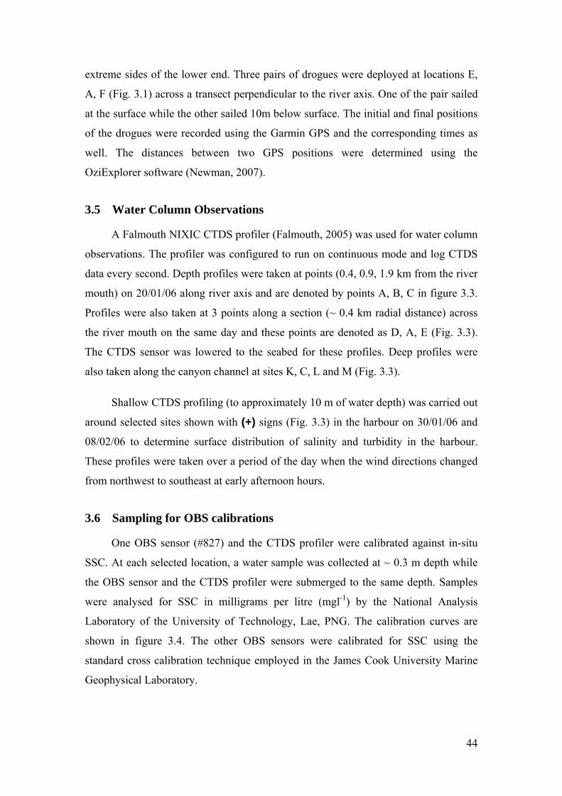
extreme sides of the lower end. Three pairs of drogues were deployed at locations E,
A, F (Fig. 3.1) across a transect perpendicular to the river axis. One of the pair sailed
at the surface while the other sailed 10m below surface. The initial and final positions
of the drogues were recorded using the Garmin GPS and the corresponding times as
well. The distances between two GPS positions were determined using the
OziExplorer software (Newman, 2007).
3.5 Water Column Observations
A Falmouth NIXIC CTDS profiler (Falmouth, 2005) was used for water column
observations. The profiler was configured to run on continuous mode and log CTDS
data every second. Depth profiles were taken at points (0.4, 0.9, 1.9 km from the river
mouth) on 20/01/06 along river axis and are denoted by points A, B, C in figure 3.3.
Profiles were also taken at 3 points along a section (~ 0.4 km radial distance) across
the river mouth on the same day and these points are denoted as D, A, E (Fig. 3.3).
The CTDS sensor was lowered to the seabed for these profiles. Deep profiles were
also taken along the canyon channel at sites K, C, L and M (Fig. 3.3).
Shallow CTDS profiling (to approximately 10 m of water depth) was carried out
around selected sites shown with (+) signs (Fig. 3.3) in the harbour on 30/01/06 and
08/02/06 to determine surface distribution of salinity and turbidity in the harbour.
These profiles were taken over a period of the day when the wind directions changed
from northwest to southeast at early afternoon hours.
3.6 Sampling for OBS calibrations
One OBS sensor (#827) and the CTDS profiler were calibrated against in-situ
SSC. At each selected location, a water sample was collected at ~ 0.3 m depth while
the OBS sensor and the CTDS profiler were submerged to the same depth. Samples
were analysed for SSC in milligrams per litre (mgl-1) by the National Analysis
Laboratory of the University of Technology, Lae, PNG. The calibration curves are
shown in figure 3.4. The other OBS sensors were calibrated for SSC using the
standard cross calibration technique employed in the James Cook University Marine
Geophysical Laboratory.
44
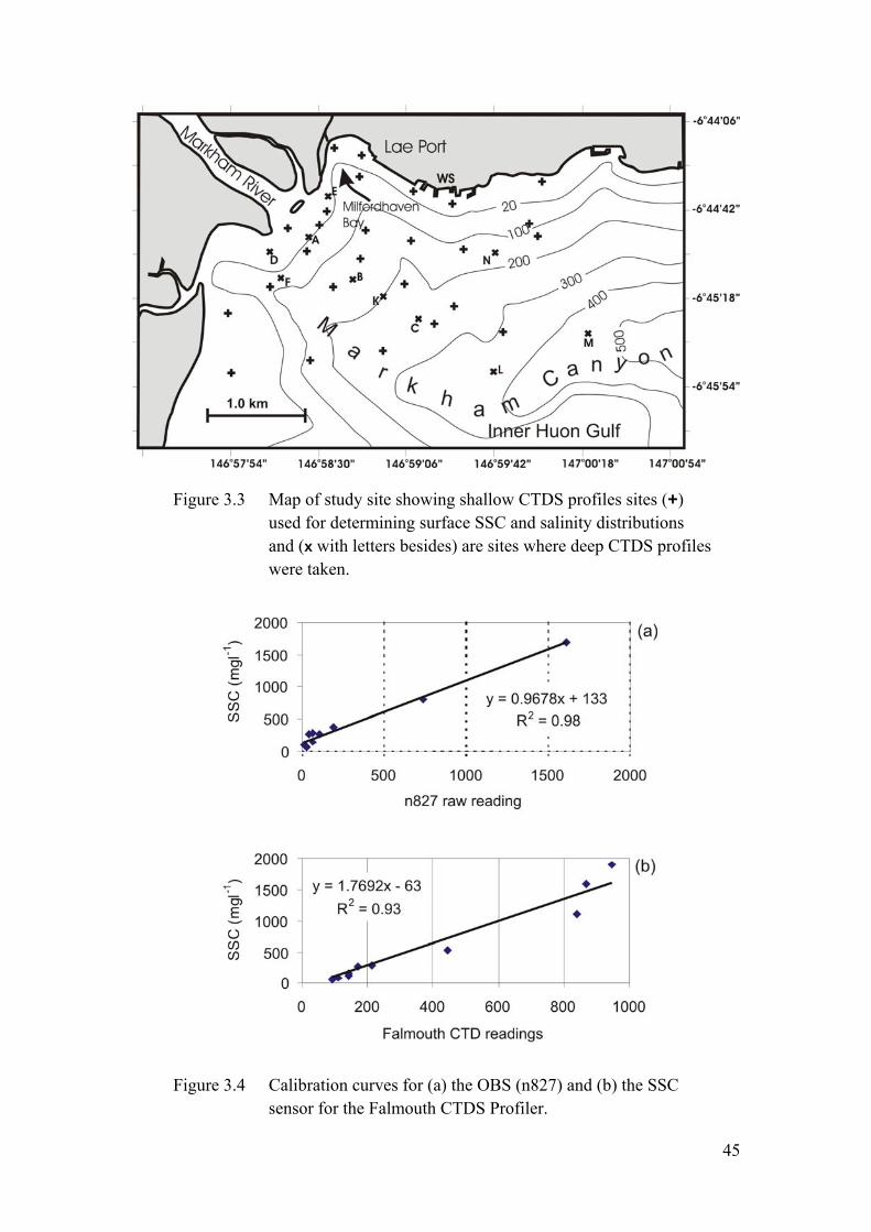
Figure 3.3 Map of study site showing shallow CTDS profiles sites (+) used for determining surface SSC and salinity distributions and (x with letters besides) are sites where deep CTDS profiles were taken.
Figure 3.4 Calibration curves for (a) the OBS (n827) and (b) the SSC sensor for the Falmouth CTDS Profiler.
45

3.7 Data Processing and Reduction
The measurements of OBS sensors and the SSC sensor for the CTDS Profiler
were calibrated against SSC and the raw calibrated data presented. The InterOcean S4
data was downloaded from the instrument as magnitude and direction of velocity and
presented. The CTD data was downloaded and processed using the CTDPro software
(Falmouth, 2005) and presented as salinity (ppt), temperature (oC) and depth (m). The
ADCP raw data for both currents and waves were downloaded using the AquaPro
software (Nortek, 2005) but the processing was done using the Storm software
(Nortek, 2005) which presents data used for interpreting currents and waves. All data
presented here was calibrated data and any reduction was therefore not necessary.
46
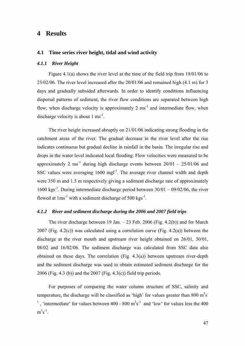
47
4 Results
4.1 Time series river height, tidal and wind activity
4.1.1 River Height
Figure 4.1(a) shows the river level at the time of the field trip from 19/01/06 to
23/02/06. The river level increased after the 20/01/06 and remained high (4.1 m) for 3
days and gradually subsided afterwards. In order to identify conditions influencing
dispersal patterns of sediment, the river flow conditions are separated between high
flow, when discharge velocity is approximately 2 ms-1 and intermediate flow, when
discharge velocity is about 1 ms-1.
The river height increased abruptly on 21/01/06 indicating strong flooding in the
catchment areas of the river. The gradual decrease in the river level after the rise
indicates continuous but gradual decline in rainfall in the basin. The irregular rise and
drops in the water level indicated local flooding. Flow velocities were measured to be
approximately 2 ms-1 during high discharge events between 20/01 – 25/01/06 and
SSC values were averaging 1600 mgl-1. The average river channel width and depth
were 350 m and 1.5 m respectively giving a sediment discharge rate of approximately
1600 kgs-1. During intermediate discharge period between 30/01 – 09/02/06, the river
flowed at 1ms-1 with a sediment discharge of 500 kgs-1.
4.1.2 River and sediment discharge during the 2006 and 2007 field trips
The river discharge between 19 Jan. – 23 Feb. 2006 (Fig. 4.2(b)) and for March
2007 (Fig. 4.2(c)) was calculated using a correlation curve (Fig. 4.2(a)) between the
discharge at the river mouth and upstream river height obtained on 26/01, 30/01,
08/02 and 16/02/06. The sediment discharge was calculated from SSC data also
obtained on these days. The correlation (Fig. 4.3(a)) between upstream river-depth
and the sediment discharge was used to obtain estimated sediment discharge for the
2006 (Fig. 4.3 (b)) and the 2007 (Fig. 4.3(c)) field trip periods.
For purposes of comparing the water column structure of SSC, salinity and
temperature, the discharge will be classified as ‘high’ for values greater than 800 m3s-
1 , ‘intermediate’ for values between 400 - 800 m3s-1 and ‘low’ for values less the 400
m3s-1.
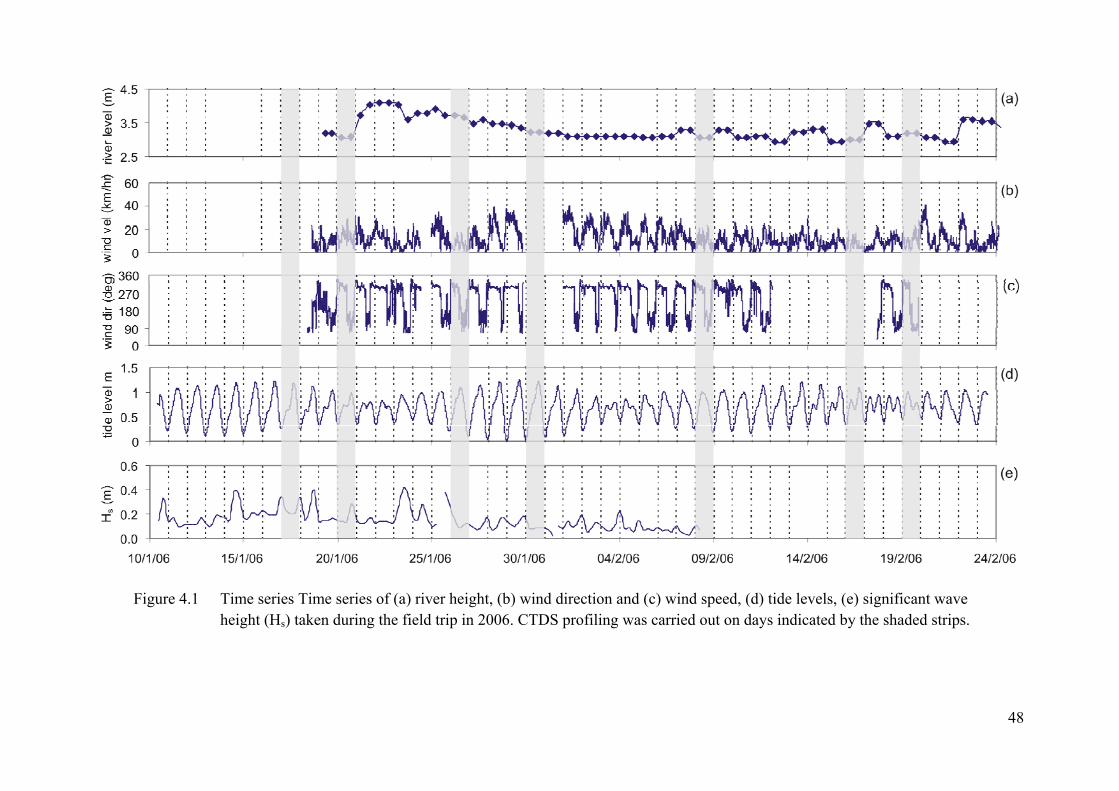
Figure 4.1 Time series Time series of (a) river height, (b) wind direction and (c) wind speed, (d) tide levels, (e) significant wave height (Hs) taken during the field trip in 2006. CTDS profiling was carried out on days indicated by the shaded strips.
48
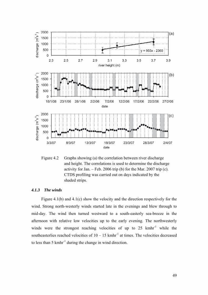
Figure 4.2 Graphs showing (a) the correlation between river discharge and height. The correlations is used to determine the discharge activity for Jan. – Feb. 2006 trip (b) for the Mar. 2007 trip (c). CTDS profiling was carried out on days indicated by the shaded strips.
4.1.3 The winds
Figure 4.1(b) and 4.1(c) show the velocity and the direction respectively for the
wind. Strong north-westerly winds started late in the evenings and blew through to
mid-day. The wind then turned westward to a south-easterly sea-breeze in the
afternoon with relative low velocities up to the early evening. The northwesterly
winds were the strongest reaching velocities of up to 25 kmhr-1 while the
southeasterlies reached velocities of 10 – 15 kmhr-1 at times. The velocities decreased
to less than 5 kmhr-1 during the change in wind direction.
49
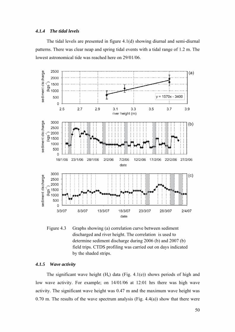
4.1.4 The tidal levels
The tidal levels are presented in figure 4.1(d) showing diurnal and semi-diurnal
patterns. There was clear neap and spring tidal events with a tidal range of 1.2 m. The
lowest astronomical tide was reached here on 29/01/06.
Figure 4.3 Graphs showing (a) correlation curve between sediment discharged and river height. The correlation is used to determine sediment discharge during 2006 (b) and 2007 (b) field trips. CTDS profiling was carried out on days indicated by the shaded strips.
4.1.5 Wave activity
The significant wave height (Hs) data (Fig. 4.1(e)) shows periods of high and
low wave activity. For example; on 14/01/06 at 12:01 hrs there was high wave
activity. The significant wave height was 0.47 m and the maximum wave height was
0.70 m. The results of the wave spectrum analysis (Fig. 4.4(a)) show that there were
50
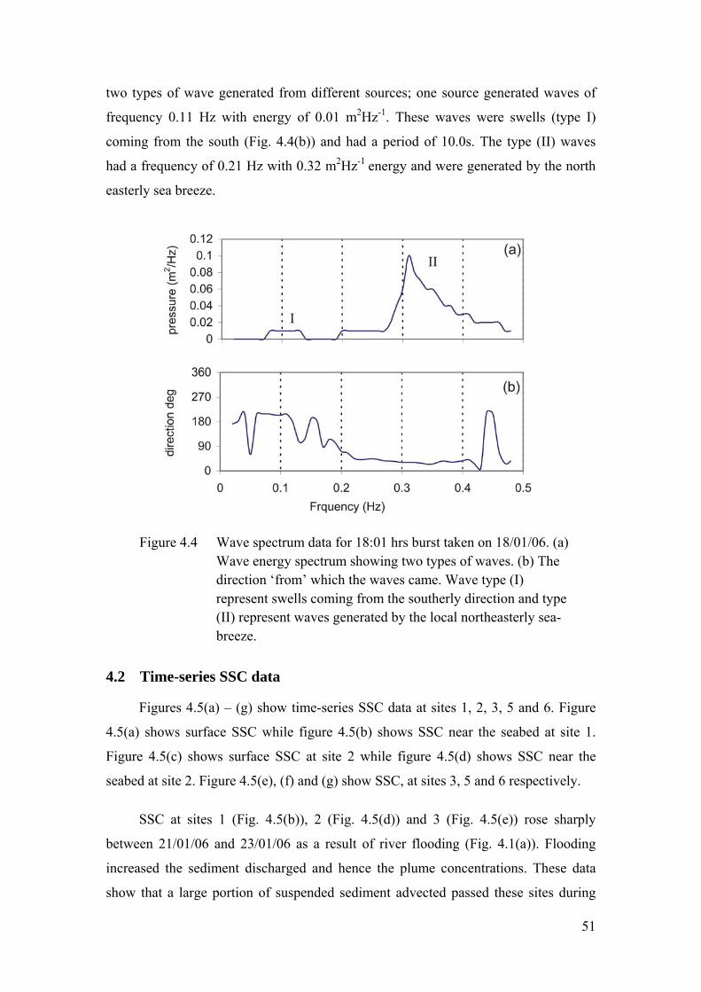
two types of wave generated from different sources; one source generated waves of
frequency 0.11 Hz with energy of 0.01 m2Hz-1. These waves were swells (type I)
coming from the south (Fig. 4.4(b)) and had a period of 10.0s. The type (II) waves
had a frequency of 0.21 Hz with 0.32 m2Hz-1 energy and were generated by the north
easterly sea breeze.
Figure 4.4 Wave spectrum data for 18:01 hrs burst taken on 18/01/06. (a) Wave energy spectrum showing two types of waves. (b) The direction ‘from’ which the waves came. Wave type (I) represent swells coming from the southerly direction and type (II) represent waves generated by the local northeasterly sea-breeze.
4.2 Time-series SSC data
Figures 4.5(a) – (g) show time-series SSC data at sites 1, 2, 3, 5 and 6. Figure
4.5(a) shows surface SSC while figure 4.5(b) shows SSC near the seabed at site 1.
Figure 4.5(c) shows surface SSC at site 2 while figure 4.5(d) shows SSC near the
seabed at site 2. Figure 4.5(e), (f) and (g) show SSC, at sites 3, 5 and 6 respectively.
SSC at sites 1 (Fig. 4.5(b)), 2 (Fig. 4.5(d)) and 3 (Fig. 4.5(e)) rose sharply
between 21/01/06 and 23/01/06 as a result of river flooding (Fig. 4.1(a)). Flooding
increased the sediment discharged and hence the plume concentrations. These data
show that a large portion of suspended sediment advected passed these sites during
51
52
the floods. It is also noted that the SSC near the sea bed was about 10 times greater
than at the surface at sites 1 and 2 during the flood. Figure 4.5(c) represents surface
turbidity data at site 2 which shows lower average SSC at the surface compared to the
surface SSC at site 1 (Fig. 4.5(a)).
Figure 4.5(e) presents sea-bed SSC at site 3. The SSC values increased to about
600 mgl-1 during the flood. This material could possibly be a combination of
sediments settling from the surface plume or be advected from the river mouth.
Figure 4.5(f) and 4.5(g) show SSC for sites 5 and 6 respectively. Site 5 was
closer to the river mouth and in shallow water (4 m) and was in the path of the
southward outflow of the river discharge. This may explain the higher SSC values at
site 5 compared to site 6 which was further away from the river mouth (Fig. 3.1).
During a time of low discharge from 15/01/ - 18/01/06 and before the floods began on
20/01/06, SSC values at site 5 exceeded values of 1400 mgl-1 while relative increases
were observed at site 6. This high turbid activity is attributed to wave action.
Concurrent wave activity during this period was high (Fig. 4.1(e)).
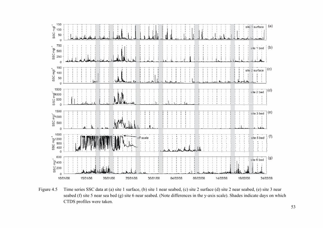
53
Figure 4.5 Time series SSC data at (a) site 1 surface, (b) site 1 near seabed, (c) site 2 surface (d) site 2 near seabed, (e) site 3 near seabed (f) site 5 near sea bed (g) site 6 near seabed. (Note differences in the y-axis scale). Shades indicate days on which CTDS profiles were taken.
4.3 Current Data
The current data collected around the harbour was needed to assist with
determining the general current pattern particularly in the 2 km vicinity of the river
mouth and the Lae Harbour. Although the ADCP was deployed for the 6 week period,
the only reliable data for current profiles measured at site 1 were obtained between
31/01/06 and 08/02/06. Drogues were used on various days especially around the
vicinity of the river mouth and just offshore of the Lae port.
4.3.1 Current profiles at site 1
Times series current velocity (Fig. 4.6(a)) for cell 7 (at sea surface) shows
relative higher velocities (~ 0.15 – 0.20 ms-1) were occurring around 00:00 hrs
between 31/02 and 04/02/06. The direction of flow at cell 7 (Fig. 4.6(b) was from the
east to west during high velocity currents. The velocity (Fig. 4.6(c)) and direction
(Fig. 4.6(d)) for cell 1 nearest to the seabed indicate smaller currents (< 0.1 ms-1) with
vague directions.
The highest currents recorded by the ADCP at site 1 were taken during the low
tides between 31/01 and 02/02/06. The velocity profiles with 1 m vertical bins taken
on 01/02/06 are shown in figure 4.7. The velocities ranged between 0.05 – 0.10 ms-1
(Fig. 4.7(a)) over the water column and were flowing from the east to the west (Fig.
4.7(b)). The currents nearest to the seabed had velocities less than 0.05 ms-1 and were
flowing generally from the south with variations in direction between the east and the
west (Fig. 4.7(b)).
Current profiles taken during the high tide show low speeds (Fig. 4.8(a)), about
ms-1, flowing to the southeast at the surface and southwest near the bed (Fig.
b)). Profiles taken during strong north-westerly winds and high tides show current
cities (Fig. 4.9(a)) around 0.05 ms-1 and flowing to the south (Fig. 4.9(b)).
0.05
4.8(
velo
54
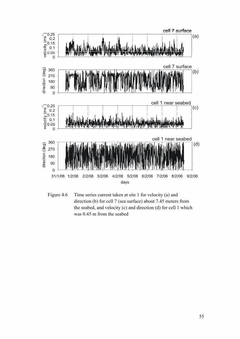
Figure 4.6 Time series current taken at site 1 for velocity (a) and direction (b) for cell 7 (sea surface) about 7.45 meters from the seabed, and velocity (c) and direction (d) for cell 1 which was 0.45 m from the seabed
55
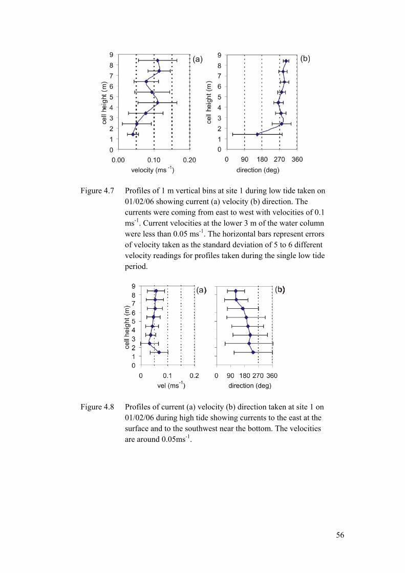
Figure 4.7 Profiles of 1 m vertical bins at site 1 during low tide taken on 01/02/06 showing current (a) velocity (b) direction. The currents were coming from east to west with velocities of 0.1 ms-1. Current velocities at the lower 3 m of the water column were less than 0.05 ms-1. The horizontal bars represent errors of velocity taken as the standard deviation of 5 to 6 different velocity readings for profiles taken during the single low tide period.
Figure 4.8 Profiles of current (a) velocity (b) direction taken at site 1 on 01/02/06 during high tide showing currents to the east at the surface and to the southwest near the bottom. The velocities are around 0.05ms-1.
56
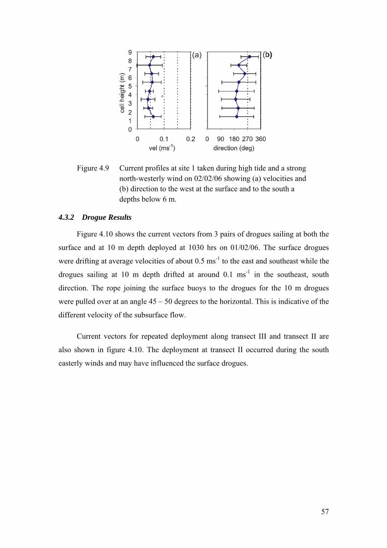
Figure 4.9 Current profiles at site 1 taken during high tide and a strong
4.3.2 Drogue Results
Figure 4.10 s th the
surface and at 10 gues
were drifting at average -1 to the east and southeast while the
drogues sailing at 10 m depth drifted at around 0.1 ms-1 in the southeast, south
direction. The rope joining the surface buoys to the drogues for the 10 m drogues
were pulled over at an angle 45 – 50 degrees to the horizontal. This is indicative of the
different velocity of the subsurface flow.
Current vectors for repeated deployment along transect III and transect II are
also shown in figure 4.10. The deployment at transect II occurred during the south
easterly winds and may have influenced the surface drogues.
north-westerly wind on 02/02/06 showing (a) velocities and (b) direction to the west at the surface and to the south a depths below 6 m.
hows the current vectors from 3 pairs of drogues sailing at bo
m depth deployed at 1030 hrs on 01/02/06. The surface dro
velocities of about 0.5 ms
57
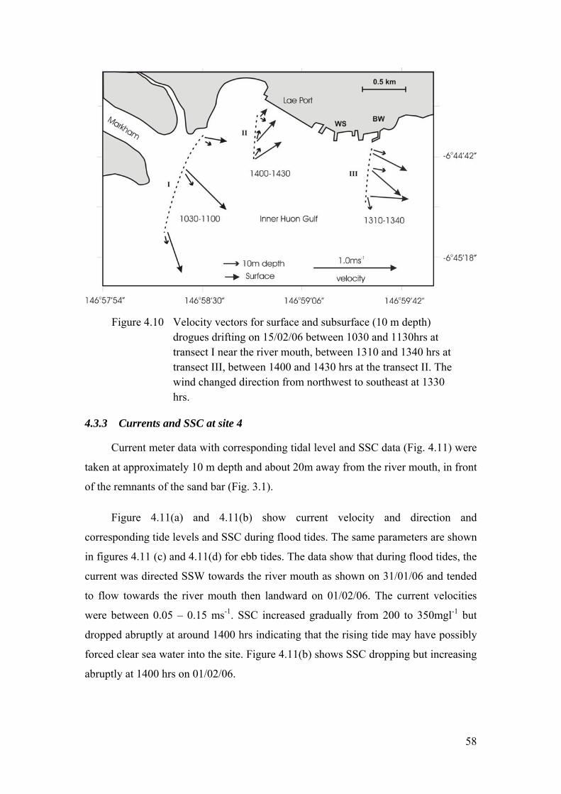
Figure 4.10 Velocity vectors for surface and subsurface (10 m depth)
level and SSC data (Fig. 4.11) were
taken at approximately 10 m depth and about 20m away from the river mouth, in front
of the
corresponding tide levels and SSC during flood tides. The same parameters are shown
in figures 4.11 (c) and 4.11(d) for ebb tides. The data show that during flood tides, the
current was directed SSW towards the river mouth as shown on 31/01/06 and tended
to flow towards the river mouth then landward on 01/02/06. The current velocities
were between 0.05 – 0.15 ms-1. SSC increased gradually from 200 to 350mgl-1 but
dropped abruptly at around 1400 hrs indicating that the rising tide may have possibly
forced clear sea water into the site. Figure 4.11(b) shows SSC dropping but increasing
abruptly at 1400 hrs on 01/02/06.
drogues drifting on 15/02/06 between 1030 and 1130hrs at transect I near the river mouth, between 1310 and 1340 hrs at transect III, between 1400 and 1430 hrs at the transect II. The wind changed direction from northwest to southeast at 1330 hrs.
4.3.3 Currents and SSC at site 4
Current meter data with corresponding tidal
remnants of the sand bar (Fig. 3.1).
Figure 4.11(a) and 4.11(b) show current velocity and direction and
58
During ebb tide as shown in figure 4.11(c) and 4.11(d), the current flow
direction was changing between the northwest and northeast but tended more
eastward during the slack low tide period. The current velocities were between 0.05 –
0.15 ms-1 and SSC was on average 200 mgl-1. The SSC on 22/02/06 gradually
increased from 100 – 200 mgl-1 with the ebbing tide.
4.3.4 CTDS profiles in the river and in close proximity outside of the river mouth
CTDS profiles inside the river show that salinity was zero (Fig. 4.12(a))
throughout the water column indicating that that there was no salt water intrusion for
all tidal levels during the field trip. The constant SSC (Fig. 4.12(b)) and temperature
(Fig. 4.12(c)) profiles show that the river water was well mixed.
Figure 4.12(d) – (f) show salinity, temperature and SSC profiles respectively,
taken a sharp
increase in salinity below
the discharge point )) at
this location indica here
were standing waves, with approximately 1 m wave height, observed at this region
er discharge velocity was equal to the
velocity of incoming waves from the sea. This type of flow is described by the
dimen
along the river axis, 10m outside of the river mouth. These results show
and temperature indicating the ambient seawater properties
. The SSC dropped to values less than 200 mgl-1 (Fig. 4.12(c
ting that sediment was settling through the water column. T
occasionally indicating a situation were the riv
sionless Froude number equaling to one.
59
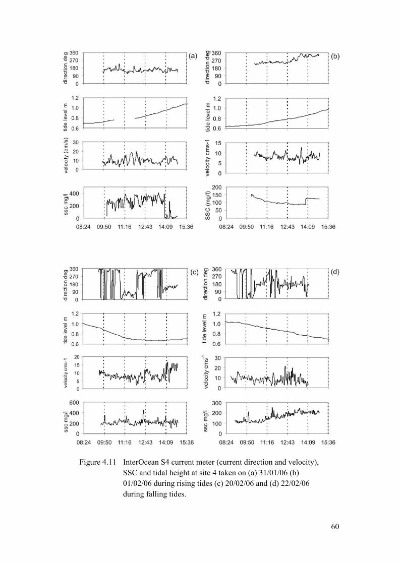
Figure 4.11 InterOcean S4 current meter (current direction and velocity), SSC and tidal height at site 4 taken on (a) 31/01/06 (b) 01/02/06 during rising tides (c) 20/02/06 and (d) 22/02/06 during falling tides.
60
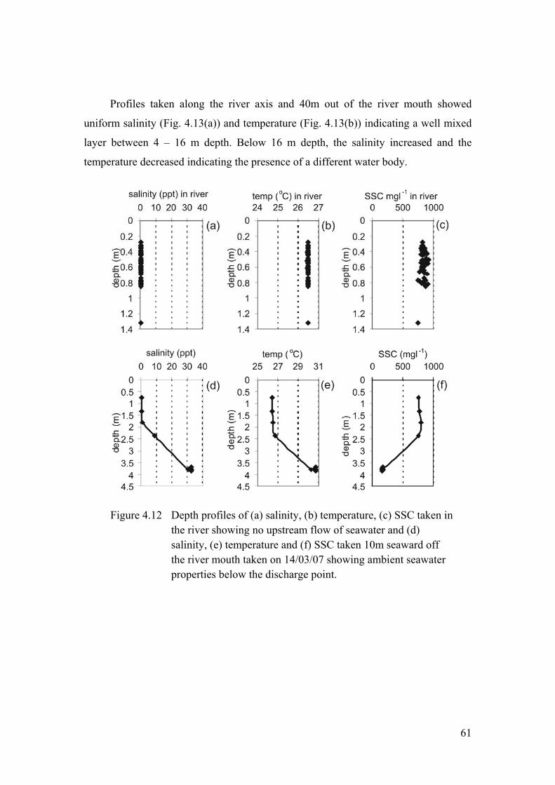
Profiles taken along the river axis and 40m out of the river mouth showed
uniform salinity (Fig. 4.13(a)) and temperature (Fig. 4.13(b)) indicating a well mixed
layer between 4 – 16 m depth. Below 16 m depth, the salinity increased and the
temperature decreased indicating the presence of a different water body.
Figure 4.12 Depth profiles of (a) salinity, (b) temperature, (c) SSC taken in the river showing no upstream flow of seawater and (d) salinity, (e) temperature and (f) SSC taken 10m seaward off the river mouth taken on 14/03/07 showing ambient seawater properties below the discharge point.
61
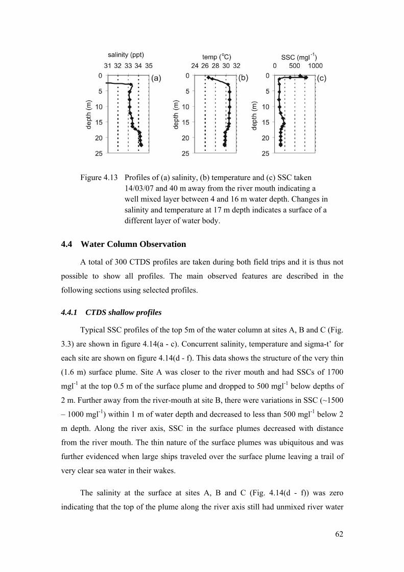
Figure 4.13 Profiles of (a) salinity, (b) temperature and (c) SSC taken 14/03/07 and 40 m away from the river mouth indicating a well mixed layer between 4 and 16 m water depth. Changes in salinity and temperature at 17 m depth indicates a surface of a different layer of water body.
4.4 Water Column Observation
A total of 300 CTDS profiles are taken during both field trips and it is thus not
possible to show all profiles. The main observed features are described in the
following sections using selected profiles.
4.4.1 CTDS shallow profiles
Typical SSC profiles of the top 5m of the water column at sites A, B and C (Fig.
3.3) are shown in figure 4.14(a - c). Concurrent salinity, temperature and sigma-t’ for
each site are shown on figure 4.14(d - f). This data shows the structure of the very thin
(1.6 m 00
mgl-1 at the top 0.5 depths of
2 m. Further away 1500
– 1000 mgl-1) with
m depth. Along the river axis, SSC in the surface plumes decreased with distance
from the river mouth. The thin nature of the surface plumes was ubiquitous and was
further evidenced when large ships traveled over the surface plume leaving a trail of
very clear sea water in their wakes.
The salinity at the surface at sites A, B and C (Fig. 4.14(d - f)) was zero
indicating that the top of the plume along the river axis still had unmixed river water
) surface plume. Site A was closer to the river mouth and had SSCs of 17
m of the surface plume and dropped to 500 mgl-1 below
from the river-mouth at site B, there were variations in SSC (~
in 1 m of water depth and decreased to less than 500 mgl-1 below 2
62

as far as site C which was about 2 km away from the river mouth. The vertical salinity
gradient was nearly linear at site A (Fig. 4.14(d)) indicating mixing. However, further
away from the river mouth at site B (Fig. 4.14(e)), there was a layer of constant
salinity at about 1.6 m depth which extended to site C (1.0 m depth) (Fig. 4.14(f))
indicating a halocline. The SSC values at this level (Fig. 4.14(a)-(c)) dropped sharply.
Figure 4.14 Shallow CTDS data recorded on 20/01/06 showing (a) near surface SSC profiles at sites (a) A, (b) B and (c) C. Concurrent (d) salinity (ppt), (e) temperature (oC) and (f) sigma-t’ (kgm-3) profiles are also shown.
4.4.2 Surface turbidity and salinity distribution
Contour maps of surface SSC (Fig. 4.15) and salinity (Fig. 4.16) distribution
were made using the data averaged over a depth of 0.5 m from each of the shallow
profiles collected on 30/01/06. Contour maps for data collected on 08/02/06 are
63
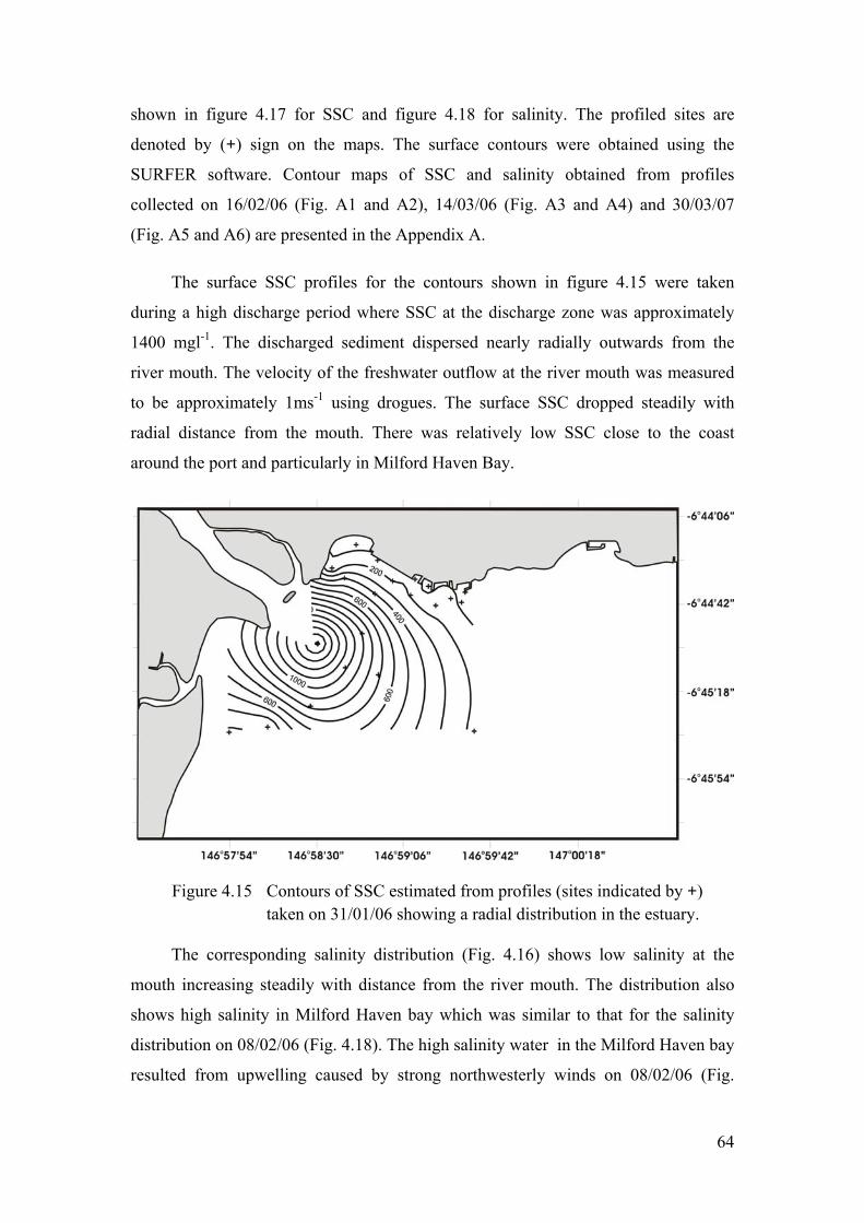
shown in figure 4.17 for SSC and figure 4.18 for salinity. The profiled sites are
denoted by (+) sign on the maps. The surface contours were obtained using the
SURFER software. Contour maps of SSC and salinity obtained from profiles
collected on 16/02/06 (Fig. A1 and A2), 14/03/06 (Fig. A3 and A4) and 30/03/07
(Fig. A5 and A6) are presented in the Appendix A.
The surface SSC profiles for the contours shown in figure 4.15 were taken
during a high discharge period where SSC at the discharge zone was approximately
1400 mgl-1. The discharged sediment dispersed nearly radially outwards from the
river mouth. The velocity of the freshwater outflow at the river mouth was measured
to be approximately 1ms-1 using drogues. The surface SSC dropped steadily with
radial distance from the mouth. There was relatively low SSC close to the coast
around the port and particularly in Milford Haven Bay.
Figure 4.15 Contours of SSC estimated from profiles (sites indicated by taken on 31/01/06 showing a radial distribution in the estu
distribution (Fig. 4.16) sh
+) ary.
The corresponding salinity ows low salinity at the
river mouth. The distribution also
shows high salin
mouth increasing steadily with distance from the
ity in Milford Haven bay which was similar to that for the salinity
distribution on 08/02/06 (Fig. 4.18). The high salinity water in the Milford Haven bay
resulted from upwelling caused by strong northwesterly winds on 08/02/06 (Fig.
64
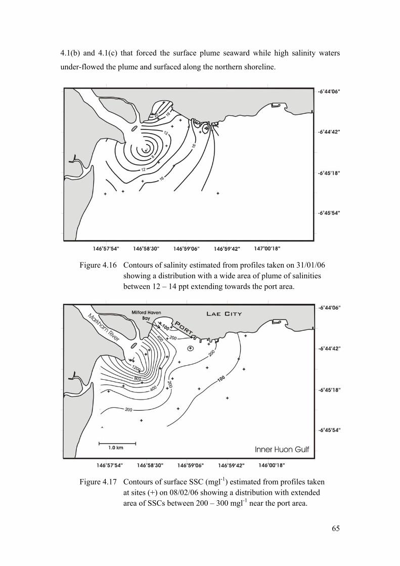
4.1(b) and 4.1(c) that forced the surface plume seaward while high salinity waters
under-flowed the plume and surfaced along the northern shoreline.
Figure 4.16 Contours of salinity estimated from profiles taken on 31/01/06 showing a distribution with a wide area of plume of salinities between 12 – 14 ppt extending towards the port area.
Figure 4.17 Contours of surface SSC (mgl-1) estimated from profiles taken at sites (+) on 08/02/06 showing a distribution with extended area of SSCs between 200 – 300 mgl-1 near the port area.
65
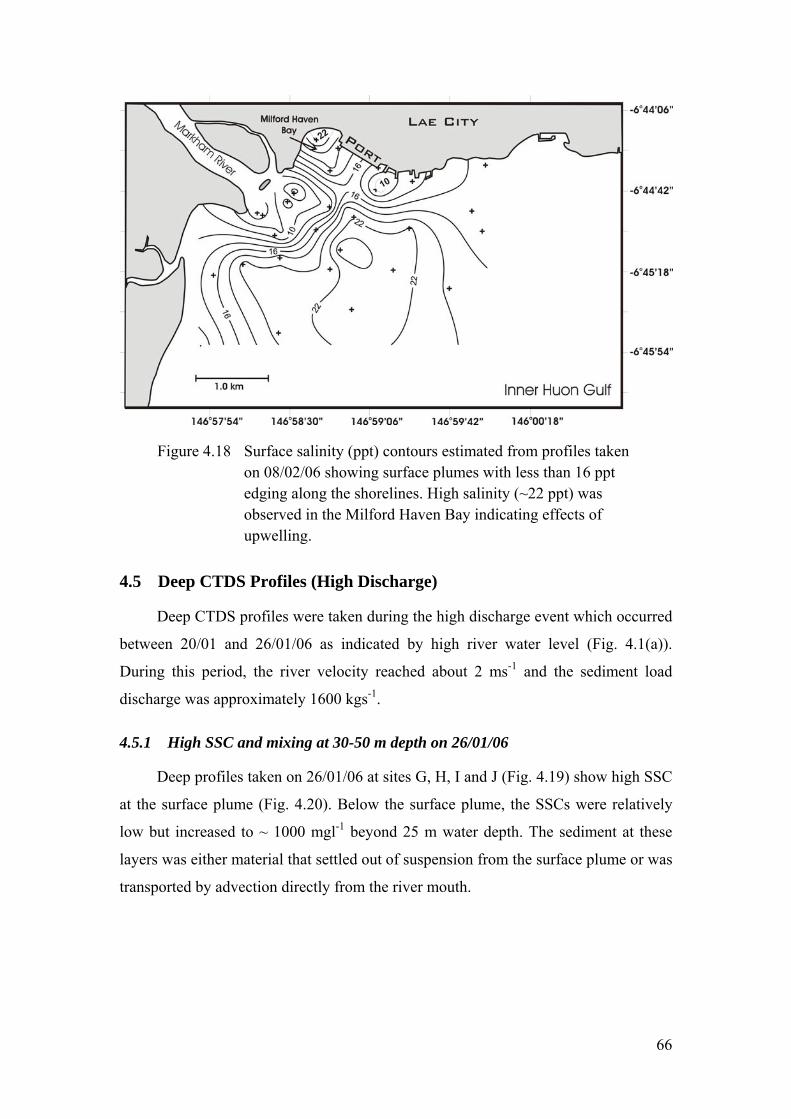
Figure 4.18 Surface salinity (ppt) contours estimated from profiles taken on 08/02/06 showing surface plumes with less than 16 ppt edging along the shorelines. High salinity (~22 ppt) was
4.5 Deep CTDS Profiles (High Discharge)
Deep CTDS profiles were taken during the high discharge event which occurred
between 20/01 and 26/01/06 as indicated by high river water level (Fig. 4.1(a)).
During this period, the river velocity reached about 2 ms-1 and the sediment load
discharge was approximately 1600 kgs-1.
4.5.1 High SSC and mixing at 30-50 m depth on 26/01/06
Deep profiles taken on 26/01/06 at sites G, H, I and J (Fig. 4.19) show high SSC
at the surface plume (Fig. 4.20). Below the surface plume, the SSCs were relatively
low but increased to ~ 1000 mgl-1 beyond 25 m water depth. The sediment at these
layers was either material that settled out of suspension from the surface plume or was
transported by advection directly from the river mouth.
observed in the Milford Haven Bay indicating effects of upwelling.
66
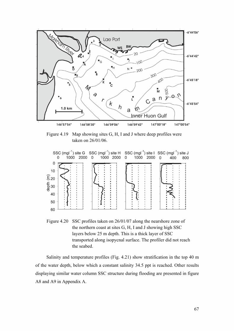
Figure 4.19 Map showing sites G, H, I and J where deep profiles were taken on 26/01/06.
Figure 4.20 SSC profiles taken on 26/01/07 along the nearshore zone of
ppt is reached. Other results
displaying similar water column SSC structure during flooding are presented in figure
A8 and A9 in Appendix A.
the northern coast at sites G, H, I and J showing high SSC layers below 25 m depth. This is a thick layer of SSC transported along isopycnal surface. The profiler did not reach the seabed.
Salinity and temperature profiles (Fig. 4.21) show stratification in the top 40 m
of the water depth, below which a constant salinity 34.5
67
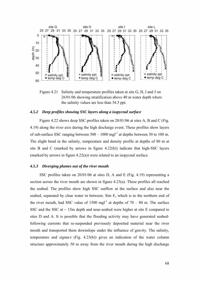
Figure 4.21 Salinity and temperature profiles taken at site G, H, I and J on 26/01/06 showing stratification above 40 m water depth where the salinity values are less than 34.5 ppt.
4.5.2
Figure 4.22 shows deep SSC profiles taken on 20/01/06 at sites A, B and C (Fig.
4.19) along the river axis during the high discharge event. These profiles show layers
of sub-surface SSC ranging between 500 – 1000 mgl-1 at depths between 30 to 100 m.
The slight bend in the salinity, temperature and density profile at depths of 80 m at
site B and C (marked by arrows in figure 4.22(b)) indicate that high-SSC layers
(marked by arrows in figure 4.22(a)) were related to an isopycnal surface.
4.5.3 Diverging plumes out of the river mouth
SSC profiles taken on 20/01/06 at sites D, A and E (Fig. 4.19) representing a
section across the river mouth are shown in figure 4.23(a). These profiles all reached
the se ar the
seabed, separated b end of
the river mouth, h ace
SSC and the SSC a th and near-seabed were higher at site E compared to
sites
ig. 4.23(b)) gives an indication of the water column
structure approximately 50 m away from the river mouth during the high discharge
Deep profiles showing SSC layers along a isopycnal surface
abed. The profiles show high SSC outflow at the surface and also ne
y clear water in between. Site E, which is to the northern
ad SSC value of 1500 mgl-1 at depths of 70 – 80 m. The surf
t ~ 15m dep
D and A. It is possible that the flooding activity may have generated seabed-
following currents that re-suspended previously deposited material near the river
mouth and transported them downslope under the influence of gravity. The salinity,
temperature and sigma-t (F
68
event. A profile taken on 20/01/06 about 1 km south of the river mouth with a distinct
high SSC bottom nepheloid layer is shown in figure A11 in Appendix A.
Figure 4.22 (a) SSC (mgl ) profiles for sites A, B and C (Fig. 4.14) along the river axis, (b) concurrent salinity (ppt), temperature (oC) and sigma-t’ (kgm-3) all recorded on 20/01/06 during a period of high discharge. The arrows indicate an isopycnal surface where layers of high SSC (1000 mgl-1) existed.
4.5.4 Deep profiles taken in 2007
The Markham River sediment discharge during the 2007 field trip (Fig. 4.3(c))
increased towards the end of the deployment period. However, before the high
discharge event that occurred on the 26/03/07, SSC profiles were collected on
23/03/07 during intermediate discharge (Fig. 4.24(a)) taken at sites C, K, L and M
-1
(see figure 4.19 for site locations). Deep profiles were again taken at the same sites 2
69
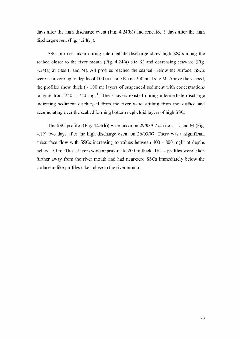
days after the high discharge event (Fig. 4.24(b)) and repeated 5 days after the high
discharge event (Fig. 4.24(c)).
SSC profiles taken during intermediate discharge show high SSCs along the
seabed closer to the river mouth (Fig. 4.24(a) site K) and decreasing seaward (Fig.
4.24(a) at sites L and M). All profiles reached the seabed. Below the surface, SSCs
were near zero up to depths of 100 m at site K and 200 m at site M. Above the seabed,
the profiles show thick (~ 100 m) layers of suspended sediment with concentrations
ranging from 250 – 750 mgl-1. These layers existed during intermediate discharge
indicating sediment discharged from the river were settling from the surface and
accumulating over the seabed forming bottom nepheloid layers of high SSC.
The SSC profiles (Fig. 4.24(b)) were taken on 29/03/07 at site C, L and M (Fig.
4.19) two days after the high discharge event on 26/03/07. There was a significant
subsurface flow with SSCs increasing to values between 400 - 800 mgl-1 at depths
below 150 m. These layers were approximate 200 m thick. These profiles were taken
further away from the river mouth and had near-zero SSCs immediately below the
surface unlike profiles taken close to the river mouth.
70
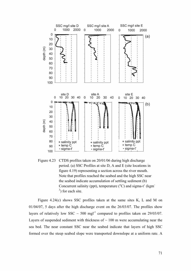
Figure 4.23 CTDS profiles taken on 20/01/06 during high discharge period. (a) SSC Profiles at site D, A and E (site locations in figure 4.19) representing a section across the river mouth. Note that profiles reached the seabed and the high SSC near the seabed indicate accumulation of settling sediment (b) Concurrent salinity (ppt), temperature (oC) and sigma-t’ (kgm-
3) for each site.
Figure 4.24(c) shows SSC profiles taken at the same sites K, L and M on
01/04/07, 5 days after the high discharge event on the 26/03/07. The profiles show
layers of relatively low SSC ~ 500 mgl-1 compared to profiles taken on 29/03/07.
Layers of suspended sediment with thickness of ~ 100 m were accumulating near the
sea bed. The near constant SSC near the seabed indicate that layers of high SSC
formed over the steep seabed slope were transported downslope at a uniform rate. A
71
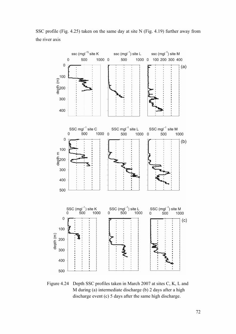
SSC profile (Fig. 4.25) taken on the same day at site N (Fig. 4.19) further away from
the river axis
Figure 4.24 Depth SSC profiles taken in March 2007 at sites C, K, L and M during (a) intermediate discharge (b) 2 days after a high discharge event (c) 5 days after the same high discharge.
72
and near the coastal shallow waters (~150 m) did not show any layers of high SSC
indicating that the deep water SSC layers were confined to the Markham canyon.
Figure 4.25 SSC profile taken on 30/03/07 at site N (Fig. 4.19) near to the northern coast at 150 m depth showing near-zero SSC in the water column indicating that sediment layers with high SSC (Fig. 4.24) are maintained in the canyon.
4.6 Deep Profiles (Intermediate Discharge)
Figure 4.26(a) shows depth SSC profiles taken at sites A, B and K (see figure
4.19 for site locations) along the river axis during a period of intermediate discharge.
The velocity at the river mouth was measured to be about 1 ms-1 and a discharge of
about 500 m3s-1. These curves indicate that the surface plumes had high SSC at site A
near the river mouth, and comparable with SSC at the same site during high discharge
events (Fig. 4.23(a)). Below the surface however, there was low SSC, less than 500
mgl-1 (Fig. 4.26(a) site A and site B) near the river mouth during periods of
intermediate discharge unlike the profiles taken during high discharge (Fig. 4.22(a)
site A and B) which showed SSC greater than 500 mgl-1 to depths of 100 m. Although
SSC values were smaller in the water column near the river mouth during
intermediate discharge, this indicates that material was still settling from the surface
and accumulating near the seabed, potentially forming high SSC bottom nepheloid
layers (Kineke et al., 1996).
linity
gradient at the surf ite A and
between 5 and 20 m at sites B and K, below which there was a halocline. Changes in
The salinity and temperature profiles (Fig. 4.26(b)) show a linear sa
ace. A well mixed layer existed between 5 and 10 m at s
73
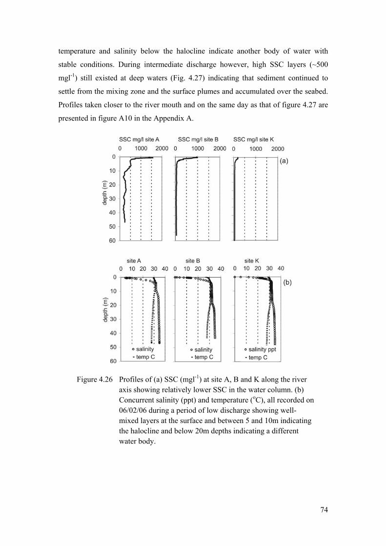
temperature and salinity below the halocline indicate another body of water with
stable conditions. During intermediate discharge however, high SSC layers (~500
mgl-1) still existed at deep waters (Fig. 4.27) indicating that sediment continued to
settle from the mixing zone and the surface plumes and accumulated over the seabed.
Profiles taken closer to the river mouth and on the same day as that of figure 4.27 are
presented in figure A10 in the Appendix A.
Figure 4.26 Profiles of (a) SSC (mgl-1) at site A, B and K along the river axis showing relatively lower SSC in the water column. (b) Concurrent salinity (ppt) and temperature (oC), all recorded on 06/02/06 during a period of low discharge showing well-mixed layers at the surface and between 5 and 10m indicating the halocline and below 20m depths indicating a different water body.
74
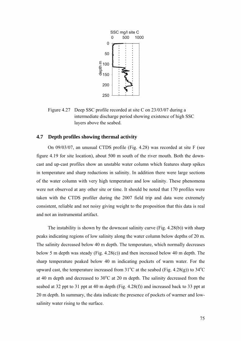
Figure 4.27 Deep SSC profile recorded at site C on 23/03/07 during a intermediate discharge period showing existence of high SSC layers above the seabed.
4.7 Depth profiles showing thermal activity
On 09/03/07, an unusual CTDS profile (Fig. 4.28) was recorded at site F (see
figure 4.19 for site location), about 500 m south of the river mouth. Both the down-
cast and up-cast profiles show an unstable water column which features sharp spikes
in temperature and sharp reductions in salinity. In addition there were large sections
of the water column with very high temperature and low salinity. These phenomena
were not observed at any other site or time. It should be noted that 170 profiles were
taken with the CTDS profiler during the 2007 field trip and data were extremely
consistent, reliable and not noisy giving weight to the proposition that this data is real
and not an instrumental artifact.
The instability is shown by the downcast salinity curve (Fig. 4.28(b)) with sharp
peaks 20 m.
The salinity decrea reases
below 5 m depth w he
sharp temperature the
upward cast, the te to 34oC
at 40 m depth and decreased to 30oC at 20 m depth. The salinity decreased from the
seabed at 32 ppt to 31 ppt at 40 m depth (Fig. 4.28(f)) and increased back to 33 ppt at
20 m depth. In summary, the data indicate the presence of pockets of warmer and low-
salinity water rising to the surface.
indicating regions of low salinity along the water column below depths of
sed below 40 m depth. The temperature, which normally dec
as steady (Fig. 4.28(c)) and then increased below 40 m depth. T
peaked below 40 m indicating pockets of warm water. For
mperature increased from 31oC at the seabed (Fig. 4.28(g))
75
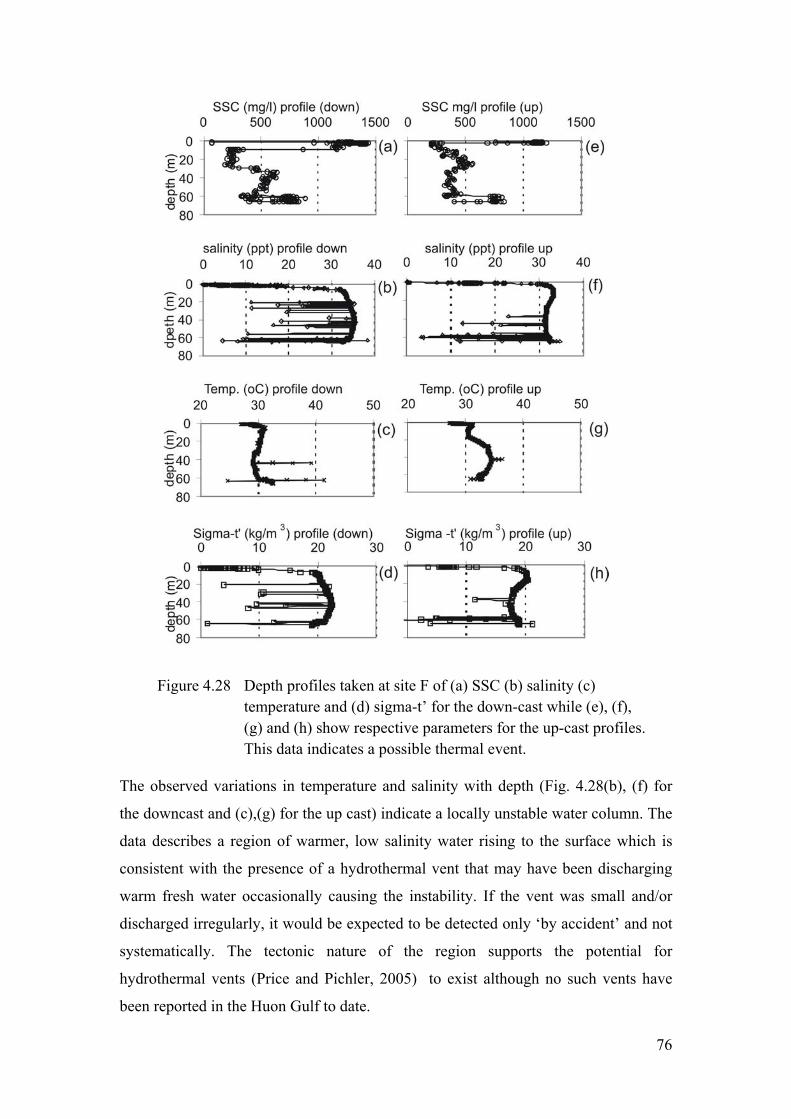
Figure 4.28 Depth profiles taken at site F of (a) SSC (b) salinity (c) temperature and (d) sigma-t’ for the down-cast while (e), (f), (g) and (h) show respective parameters for the up-cast profiles.
ate.
This data indicates a possible thermal event.
The observed variations in temperature and salinity with depth (Fig. 4.28(b), (f) for
the downcast and (c),(g) for the up cast) indicate a locally unstable water column. The
data describes a region of warmer, low salinity water rising to the surface which is
consistent with the presence of a hydrothermal vent that may have been discharging
warm fresh water occasionally causing the instability. If the vent was small and/or
discharged irregularly, it would be expected to be detected only ‘by accident’ and not
systematically. The tectonic nature of the region supports the potential for
hydrothermal vents (Price and Pichler, 2005) to exist although no such vents have
been reported in the Huon Gulf to d
76
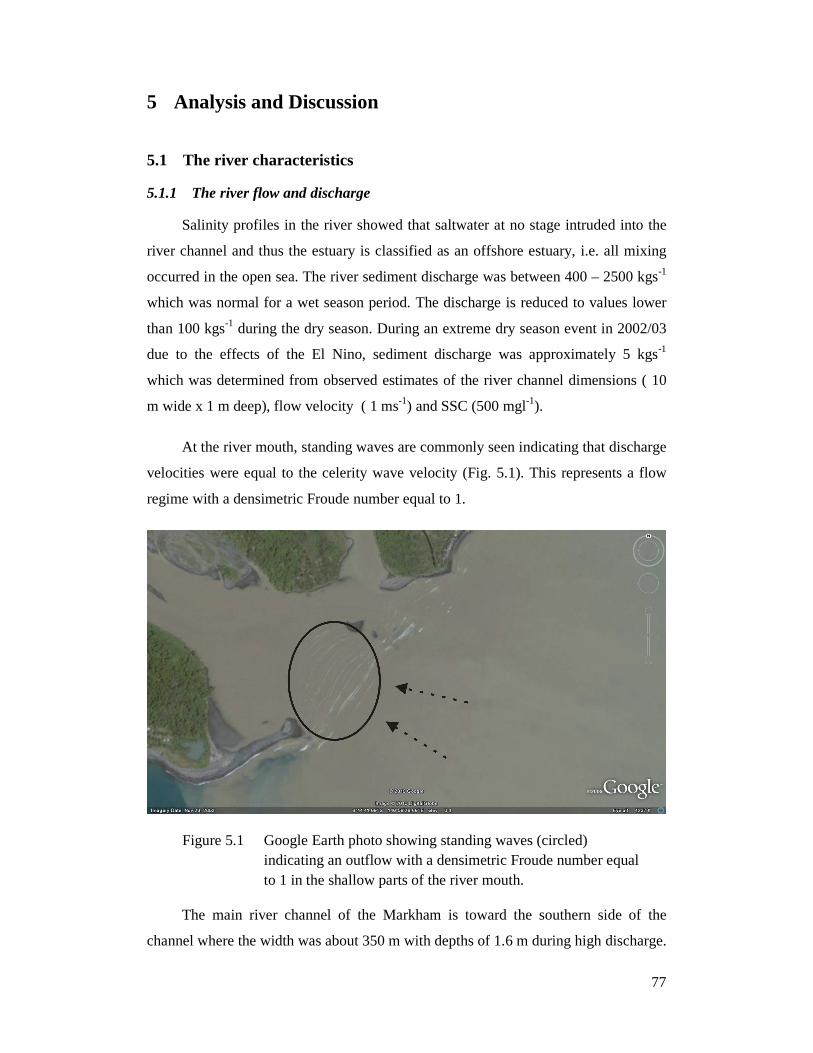
77
5 Analysis and Discussion
5.1 The river characteristics
5.1.1 The river flow and discharge
Salinity profiles in the river showed that saltwater at no stage intruded into the
river channel and thus the estuary is classified as an offshore estuary, i.e. all mixing
occurred in the open sea. The river sediment discharge was between 400 – 2500 kgs-1
which was normal for a wet season period. The discharge is reduced to values lower
than 100 kgs-1 during the dry season. During an extreme dry season event in 2002/03
due to the effects of the El Nino, sediment discharge was approximately 5 kgs-1
which was determined from observed estimates of the river channel dimensions ( 10
m wide x 1 m deep), flow velocity ( 1 ms-1) and SSC (500 mgl-1).
At the river mouth, standing waves are commonly seen indicating that discharge
velocities were equal to the celerity wave velocity (Fig. 5.1). This represents a flow
regime with a densimetric Froude number equal to 1.
Figure 5.1 Google Earth photo showing standing waves (circled) indicating an outflow with a densimetric Froude number equal to 1 in the shallow parts of the river mouth.
The main river channel of the Markham is toward the southern side of the
channel where the width was about 350 m with depths of 1.6 m during high discharge.
In the north, the remnants of the sand bar in the centre of the river mouth were
surrounded by shallow (~ 30 cm depth) water. What looks like an extra river channel
a discharge channel but has ceased to discharge
due to natural closure of the channel about 500 m upstream.
5.1.2
bedload are moved by the Markham River. The commonly assumed ratio of bedload
to sus
ped by Milliman and Syvitski
(1992) give approximately 10 Mtons which agrees well with the values given here.
The environment in Lae, PNG is prone to hazardous activity (Buleka et al.,
1999) that may generate huge quantities of both bedload and suspended load into the
Markham canyon. Episodic events include slope failure triggered by flooding or
earthquakes.
5.2 Estuarine Characteristics
The surface plume generated by the river was thin (1.6 m), formed within a few
tens of metres of the sill at the mouth of the river, and extended about 4 – 5km
offshore.
5.2.1 Riverine forcing
ct input of
momentum as well ver
the off-shore estua he baroclinic pressure
anom
in the northern end was previously
The bedload transport
It was difficult to quantify the bedload material transported out of the river,
however it is probable that a considerable bedload transport exists with material sizes
up to cobbles being common in the channel. Coarser material observed along the
canyon channel (Buleka et al., 1999) may partly be attributed to bedload material
transported down the steep slopes to deep seas.
Nedeco Haskoning and Maunsell (1980) reported that about 2 Mtons per year of
pended load is 1:10 (Allen, 1997) and estimates of the suspended load (between
9 – 12 Mtons per year) giving the Nedeco estimate reasonable. Estimates of the
discharged suspended load using algorithms develo
At the discharge point, the freshwater inflow provides a dire
as a large buoyancy force both of which contribute to motion o
ry. The buoyancy forcing is estimated from t
aly associated with the freshwater plume and given by the equation (Geyer et al.,
2000);
78
0
0( ( ))f
h
P g z dz
(5.1)
where ρo is the density of the ambient seawater and ρ(z) is the density of the
fluid at the top surface of the plume and is the thickness of the plume h = 1.6 m.
ume, equation 5.1 yields a pressure anomaly of 257 Pa
which
the momentum input from the river
(Garvine, 1995).
ff’
depth indicate that the sedim
ined into the sediment-laden river water initiating flocculation. Large
flocculated particles fall out of the fresh water plume and form a region of high SSC
ver mouth.
e fraction) at the water surface and is distributed by surface plumes. The
coarser fraction of the sediment will settle out of the mixing zone, or out of the
aterial. Water masses sinking under the influence of
mode
Using data for the Markham pl
is equivalent to 2.3 cm of sea-level displacement. This is comparable with the
observed value of 309 Pa (3.0 cm) measured for the Eel River floods (Geyer et al.,
2000). Using Bernoulli’s equation, the pressure anomaly implies a horizontal water
velocity of 0.7 ms-1, close to the measured values. This implies that dynamics in the
vicinity of the mouth is strongly influenced by
5.2.2 Separation of sediment at turbulent mixing zone
The schematic diagram of the mixing zone in figure 5.2 describes the processes
that occur when river water meets the seawater. At the point of discharge, the fast
flowing fresh water interacts with the seawater creating a turbulent mixing zone. The
drastically reduced SSC levels at depths of 2 m (Fig. 4.12(f)) and the plume ‘lift-o
ent laden freshwater, discharged at the mouth, rose above
the ambient seawater and flowed seaward. The momentum of the river flow continues
to push fresh river water over the mixing zone and beyond as surface plume. The
saltwater is entra
in the lower water column near the ri
It is in this zone, within a few tens of meters of the river mouth, that much of the
transported sediment pathways are determined. Some of the discharged sediment
remain (fin
surface plume as flocculated m
rate sediment loads may move downslope and in some instances move along
isopycnal surfaces. Water with sufficiently high sediment loads may be too dense to
find equilibrium in the water column and continue to move downslope into the deep
canyon.
79
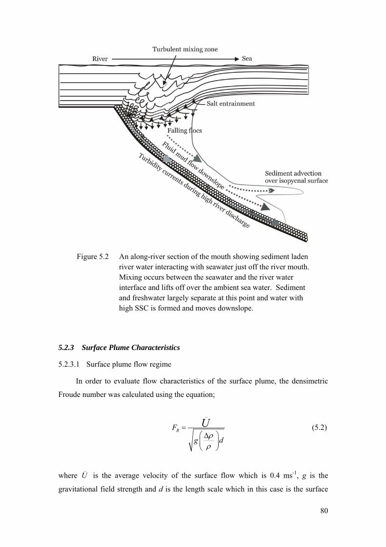
Figure 5.2 An along-river section of the mouth showing sediment laden river water interacting with seawater just off the river mouth. Mixing occurs between the seawater and the river water interface and lifts off over the ambient sea water. Sediment and freshwater largely separate at this point and water with high SSC is formed and moves downslope.
5.2.3 Surface Plume Characteristics
5.2.3.1 Surface plume flow regime
In order to evaluate flow characteristics of the surface plume, the densimetric
Froude number was calculated using the equation;
_
RF
g d
U
(5.2)
where _
U is the average velocity of the surface flow which is 0.4 ms-1, g is the
gravitational field strength and d is the length scale which in this case is the surface
80
plume thickness 1.6 m. Δρ is the change in density between the surface plume and the
ambient seawater below the plume. ρ is the density of the ambient seawater.
Substituting values in the equation gives a densimetric Froude number (FR) of 0.75
which is less the 1, implying that the surface plume flow is sub-critical. This result
emphasizes that the effect of buoyancy is very important and mixing due to the
shearing velocity is minimal (Allen, 1997).
5.2.3.2 Degree of Stratification
The degree of stratification of the estuary is characterized by Richardson’s
number R, which gives a measure of the stabilizing effect of the buoyancy to the
destabilizing effect of the vertical velocity shear (Fisher et al., 1972). R is given by;
2( / )
RdU dz
( / )( / )g d dz (5.3)
where g is the gravitational acceleration,
is the density of the ambient seawater,
dρ/dz g ocity
gradient over the su
An estimate data
presented in figure kgm-3
at site B (Fig. 4.14(e)), and with the underlying seawater at 1018 kgm-3, the change in
density was 18 kgm-3. The velocity of the plume was taken as 0.4 ms-1 (from the
lying seawater velocity was approximated at
0.05 ms . This result gives a Richardson number of 0.61, which is larger than 0.25
r interface is gravitationally stable and that the
estua
5.2.4 Subsurface Water Column Structure
5.2.4.1 Density structure
The density profiles (Fig. 4.22(b)) shows increasing density with depth
indicating a stable water column. In some instances, there were sharp changes in
water density well below the surface plume. For example, figure 4.22(b) shows a
is the chan e in density over the surface plume, and dU/dz is the vel
rface plume.
of the degree of stratification is made using measured
4.14. The density of surface plume was approximately 1000
drogue data (Fig. 4.10), and the under-1
implying that the fresh and seawate
ry can therefore be characterized as highly stratified (Fisher et al., 1972).
profile with relatively constant density at around 60m (shown by arrows) and
remaining constant until about 75 m depth where the density increased slightly but
81
sharply. This layer represented an isopycnal surface where a sub-surface sediment
plume advected horizontally with SSC values (Fig. 4.22a) of approximately 1000 mgl-
1.
5.2.4.2 Layers of sediment over the seabed
Deep SSC profiles also showed the existence of layers of sediment near the
seabed (Fig. 4.23(a) and 4.24). These layers resulted from settling of flocculated
ent mixing zone or the surface plumes. Flocculation
occur
to
the plume current and flocculate during the process, later falling out of the plumes and
settling as larger flocs.
Turbidity currents generated along the seabed slope as a negatively buoyant
plumes directly discharged from the river, were not observed or measured during this
al., 1990) which are far higher than those measured
in the
idely by the surface plumes over the
estuary (Fig. 4.15 and 4.17). However, the distribution of the surface plume varied at
occurred as a result of changes in discharge and effects of
the w
particles settling out of the turbul
red at the turbulent mixing zone within 1 – 2 minutes of the discharged
freshwater sediment mixing with the entrained saltwater, even with a salinity as small
as 1 ppt (Wolanski et al., 1995). Disaggregated material may be entrained back in
trip. This is not surprising given that the SSCs required to generate negative buoyant
plumes are 20 – 30 gl-1 (Wright et
river during this work. However, nepheloid layers with high SSC (Fig. 4.23(a)
and higher densities (Fig. 4.23(b)) observed near the seabed close to the river mouth
can flow downslope given the steep seabed slopes. This type of flow can be
considered as sediment induced downward flow. The deep profiles that reached the
seabed (Fig. 4.24) support this description.
5.3 Variations in Plume SSC
5.3.1 Dispersal by surface plumes
The sediment is generally distributed w
times and these variations
ind. The tidal range was small (< 1.2 m) and did not have a significant effect on
the surface plumes.
82
5.3.1.1 The high discharge event and its influence
The flooding during the earlier part (20/01 – 24/01/06) of the deployment in
2006 discharged sediment at approximately 1200 kgs-1. During this period there was
ept for site 6 (Fig. 3.1). SSCs at sites 1
and 2 increased from about 30 mgl to 250 mgl-1 at the surface (Fig.4.5(a) and 4.5(c))
and from
nge of only 1.2 m and a very large general water depth of
many
figure 5.3 for sites 1 and 2 on the northern coast and figure 5.4 for sites 5 and 6 on the
site locations). Surface plumes with low SSC
frequently existed at site 1 and 2 during northwesterly winds (Fig. 5.3(a) & (b)) with
winds. The SSCs at site 1 and 2 were also
influe
s between wind direction and SSC have low R values but do
corroborate visual observations that strong northwesterly winds forced the surface
plumes directly seaward leaving the coastal near-shore regions with very clear
saltwater. During low velocity northwesterly winds however, buoyancy forces,
relatively high SSC measured at all sites exc-1
50 mgl-1 and 500 mgl-1 near the seabed (Figs. 4.5(b) and 4.5(d)). The SSCs
near the seabed at site 3 was on average 600 mgl-1 during the high discharge event.
These were the only large SSC values recorded during the deployment period
responding to rising river levels due to flooding (Fig. 4.1(a)). The SSC values at all
sites after the floods were relatively low.
5.3.1.2 The tidal influence
The small tidal ra
hundreds of meters result in relatively small tidal currents (ca 0.1 m/s) and thus
transport of sediment is relatively unaffected by tides. There was however current data
(Figs. 4.6 – 4.9) at site 1 showing surface currents from the north-west with velocities
of 0.1 ms-1 between 01/02 and 03/02/06. This may indicate the direction and flow of
the surface plume which tends to follow the near-shore waters as shown in figure
4.18.
5.3.1.3 The wind influence
The wind had a significant influence on the SSC close to the coast as shown in
western coast (see figure 3.1 for
higher SSCs during southeasterly
nced by the magnitude of the northwesterly wind velocity with higher SSCs
occurring during low wind velocity (Fig. 5.3(c) & (d)). Similar effects were seen at
site 5 and 6 (Figs. 5.4(a) – (d)) on the western coast of the study area.
The correlation 2
83
overcame the low north-westerly wind forces and forced the surface plume towards
the coast, thus increasing SSC along the shoreline. The southeasterly wind forced the
surface plumes towards the nearshore zones causing SSC to increase at sites 1 and 2.
Figure 5.3 Correlation between wind direction and SSC at site 1 (a) and site 2 (b) showing higher SSC during southeasterly winds compared to lower SSC during northwesterly winds. Correlations between northwesterly wind speed and SSC for
nd for site 2 (d) show low SSC during high
orthwesterly
winds
site 1 (c) anorthwesterly wind speeds compared to high SSC during low wind speeds. This indicates that buoyancy forces dominated wind stress during weak NW winds forcing the plume towards the northern coast.
5.3.1.4 Upwelling occurring along northern coast
It is evident from the salinity distribution charts (Fig. 4.18) showing high
salinity areas in the Milford Haven Bay, that upwelling occurred close to the northern
coast. This happened as a result of strong northwesterly winds driving the surface
waters seaward leaving clean seawater in the northern coasts. When the n
subsided in the afternoons, the surface plumes edged northward and covered
the Milford Haven Bay. A Google Earth photo (Fig. 5.5) shows the clear water in
Milford Haven Bay, a pattern which was visually observed to occur virtually every
day when NW winds were blowing.
84
Figure 5.4 Correlation between wind direction and SSC at site 5 (a) and site 6 (b). SSC was relatively higher during northwesterly winds compared to SSC during southeasterly winds.
Further evide rly morning
periods during the ight.
During this period, ver
separated from the coast and was located approximately 100 m offshore, and parallel
eward as the northwesterly wind
subsided.
Correlations between northwesterly wind speed and SSC are shown for site 5 (c) and for site 6. These graphs indicate that buoyancy forces were again dominant during weak NW winds forcing the plume towards the western coast.
nce of upwelling (Fig. 5.6) was observed during the ea
continuation of strong northwesterly winds blowing overn
the northern edge of the surface plumes from the Markham Ri
with the shoreline. The plume edge moved shor
85
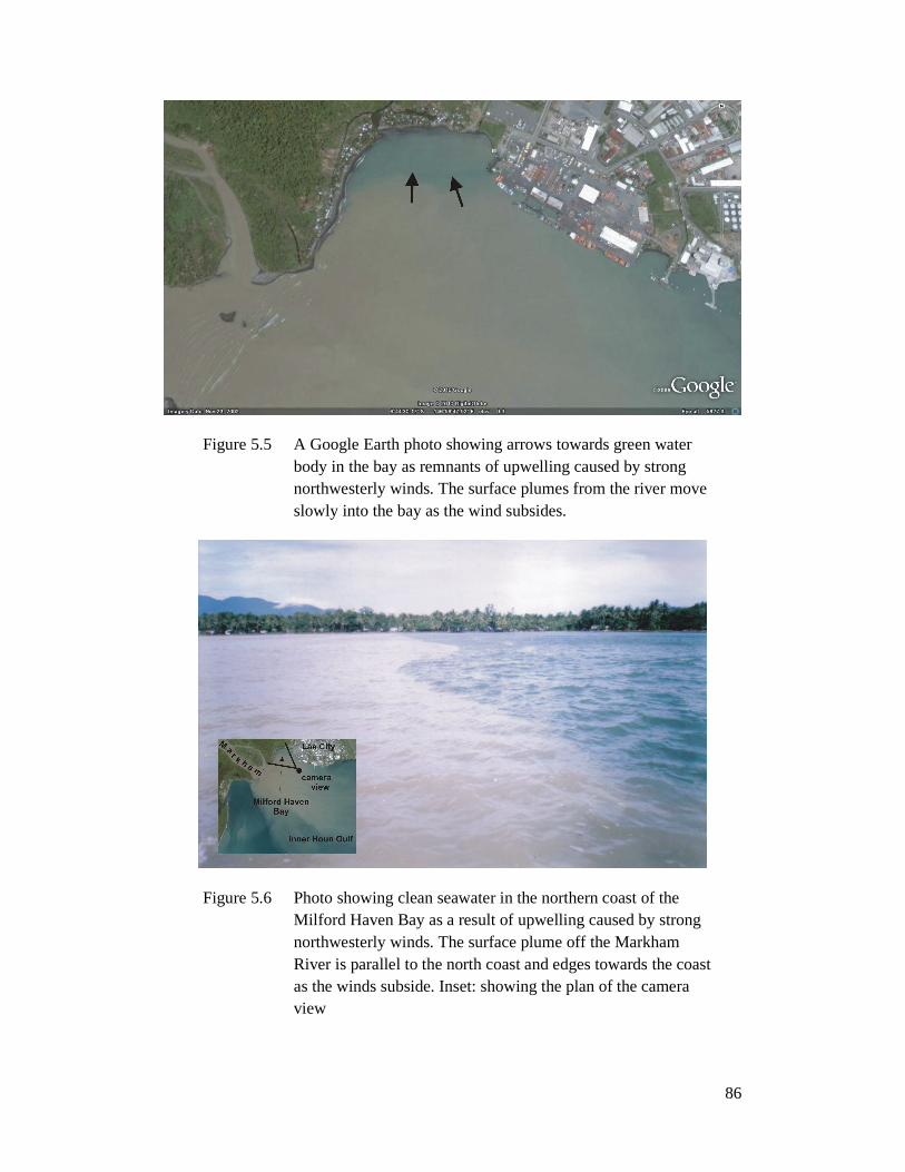
86
Figure 5.5 A Google Earth photo showing arrows towards green water body in the bay as remnants of upwelling caused by strong northwesterly winds. The surface plumes from the river move slowly into the bay as the wind subsides.
Figure 5.6 Photo showing clean seawater in the northern coast of the Milford Haven Bay as a result of upwelling caused by strong northwesterly winds. The surface plume off the Markham River is parallel to the north coast and edges towards the coast as the winds subside. Inset: showing the plan of the camera view
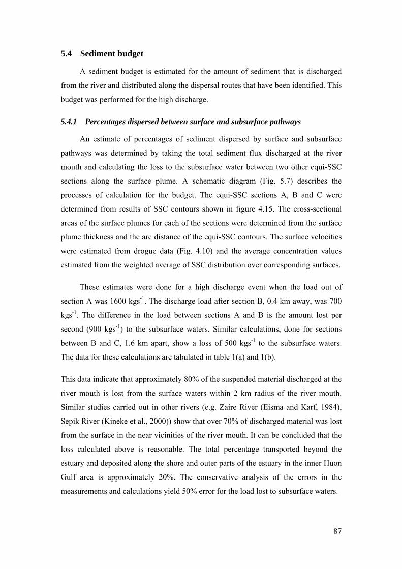
5.4 Sediment budget
A sediment budget is estimated for the amount of sediment that is discharged
from the river and distributed along the dispersal routes that have been identified. This
budget was performed for the high discharge.
5.4.1 Percentages dispersed between surface and subsurface pathways
An estimate of percentages of sediment dispersed by surface and subsurface
pathways was determined by taking the total sediment flux discharged at the river
mouth and calculating the loss to the subsurface water between two other equi-SSC
sections along the surface plume. A schematic diagram (Fig. 5.7) describes the
processes of calculation for the budget. The equi-SSC sections A, B and C were
determined from results of SSC contours shown in figure 4.15. The cross-sectional
areas of the surface plumes for each of the sections were determined from the surface
plume locities
were estimated fro lues
estimated from the ibution over corresponding surfaces.
These estimates were done for a high discharge event when the load out of
section A was 1600 kgs-1. The discharge load after section B, 0.4 km away, was 700
kgs-1. The difference in the load between sections A and B is the amount lost per
second (900 kgs-1) to the subsurface waters. Similar calculations, done for sections
between B and C, 1.6 km apart, show a loss of 500 kgs-1 to the subsurface waters.
The data for these calculations are tabulated in table 1(a) and 1(b).
This data indicate that approximately 80% of the suspended material discharged at the
river mouth is lost from the surface waters within 2 km radius of the river mouth.
Similar studies carried out in other rivers (e.g. Zaire River (Eisma and Karf, 1984),
Sepik River (Kineke et al., 2000)) show that over 70% of discharged material was lost
from the surface in the near vicinities of the river mouth. It can be concluded that the
loss c b ond the
estuary and deposit uon
Gulf area is appr in the
measurements and rs.
thickness and the arc distance of the equi-SSC contours. The surface ve
m drogue data (Fig. 4.10) and the average concentration va
weighted average of SSC distr
alculated a ove is reasonable. The total percentage transported bey
ed along the shore and outer parts of the estuary in the inner H
oximately 20%. The conservative analysis of the errors
calculations yield 50% error for the load lost to subsurface wate
87
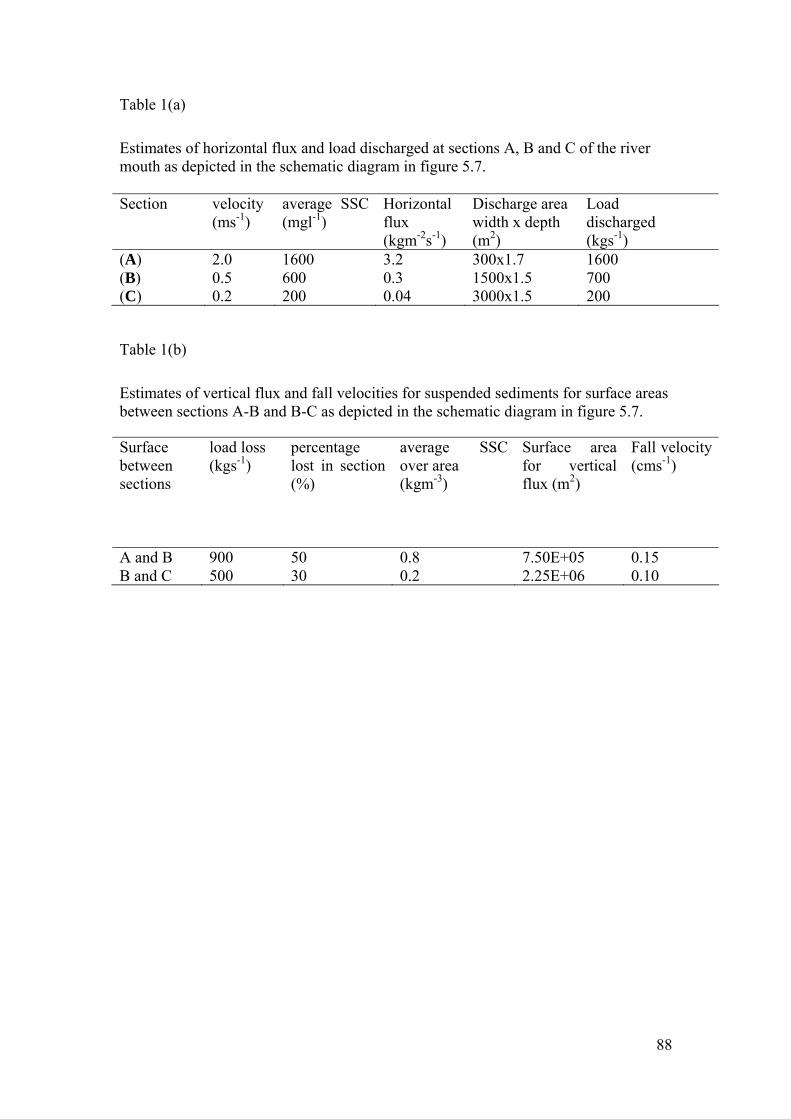
Table 1(a)
Estim
(ms-1) (mgl-1) ntal
flux Discharge area width x depth
Load discharged
s-1)
ates of horizontal flux and load discharged at sections A, B and C of the river mouth as depicted in the schematic diagram in figure 5.7. Section velocity average SSC Horizo
(kgm-2s-1) (m2) (kg(A) 2.0 1600 3.2 300x1.7 1600 (B) 0.5 600 0.3 1500x1.5 700 (C) 0.2 200 0.04 3000x1.5 200
Table 1(b)
Estimates of vertical flux and fall velocities for suspended sediments for surface areas between sections A-B and B-C as depicted in the schematic diagram in figure 5.7. Surface between sections
load loss (kgs-1)
percentage lost in section (%)
average SSC over area (kgm-3)
Surface area for vertical flux (m2)
Fall velocity(cms-1)
A and B 900 50 0.8 7.50E+05 0.15 B and C 500 30 0.2 2.25E+06 0.10
88
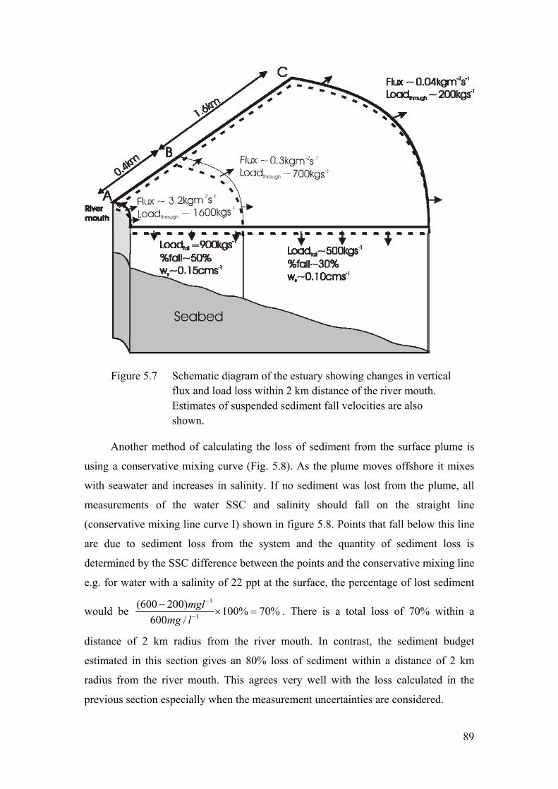
Figure 5.7 Schematic diagram of the estuary showing changes in vertical flux and load loss within m distance of t uth. Estimates of suspended sediment fall velocities are also shown.
Another method of calculating the loss of sediment from the surface plume is
using a conservative mixing curve (Fig. 5.8). As the plume moves offshore it mixes
with seawater and increases in salinity. If no sediment was lost from the plume, all
measurements of the water SSC and salinity should fall on the straight line
(conservative mixing line curve I) shown in figure 5.8. Points that fall below this line
are due to sediment loss from the system and the quantity of sediment loss is
determined by the SSC difference between the points and the conservative mixing line
e.g. for water with a salinity of 22 ppt at the surface, the percentage of lost sediment
would be
2 k he river mo
1
. There is a total loss of 70% within a
distance of 2 km outh. In contrast, the sediment budget
estimated in this section gives an 80% loss of sediment within a distance of 2 km
radius from the river mouth. This agrees very well with the loss calculated in the
previous section especially when the measurement uncertainties are considered.
1
(600 200)100% 70%
600 /
mgl
mg l
radius from the river m
89
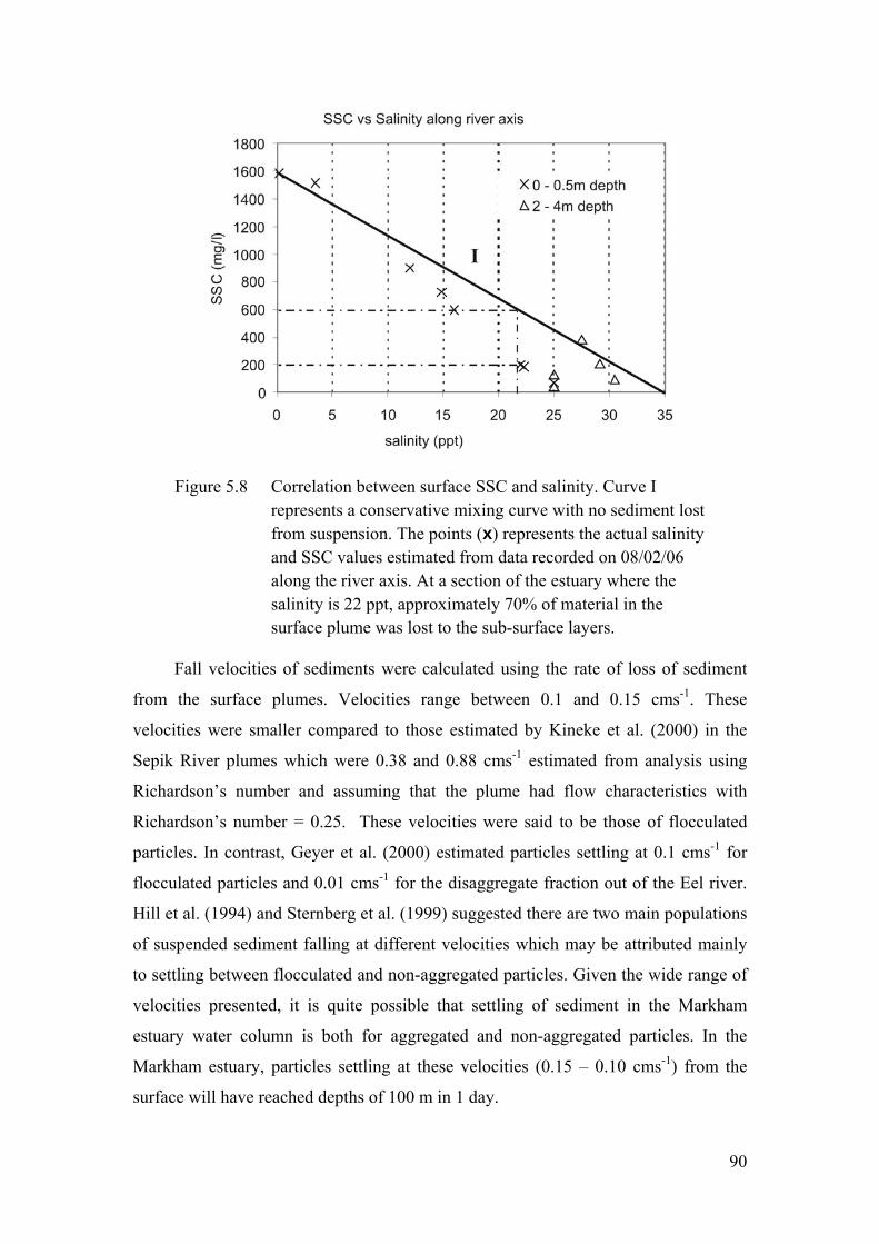
Figure 5.8 Correlation between surface SSC and salinity. Curve I represents a conservative mixing curve with no sediment lost from suspension. The points (x) represents the actual salinity and SSC values estimated from data recorded on 08/02/06
Fall velocitie ents were calculated using the rate of loss of sediment
from
of suspended sediment falling at different velocities which may be attributed mainly
etween flocculated and non-agg
along the river axis. At a section of the estuary where the salinity is 22 ppt, approximately 70% of material in the surface plume was lost to the sub-surface layers.
s of sedim
the surface plumes. Velocities range between 0.1 and 0.15 cms-1. These
velocities were smaller compared to those estimated by Kineke et al. (2000) in the
Sepik River plumes which were 0.38 and 0.88 cms-1 estimated from analysis using
Richardson’s number and assuming that the plume had flow characteristics with
Richardson’s number = 0.25. These velocities were said to be those of flocculated
particles. In contrast, Geyer et al. (2000) estimated particles settling at 0.1 cms-1 for
flocculated particles and 0.01 cms-1 for the disaggregate fraction out of the Eel river.
Hill et al. (1994) and Sternberg et al. (1999) suggested there are two main populations
to settling b regated particles. Given the wide range of
velocities presented, it is quite possible that settling of sediment in the Markham
estuary water column is both for aggregated and non-aggregated particles. In the
Markham estuary, particles settling at these velocities (0.15 – 0.10 cms-1) from the
surface will have reached depths of 100 m in 1 day.
90
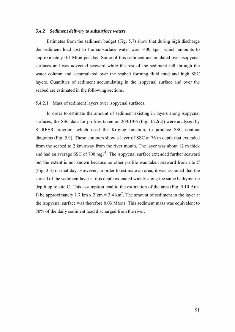
5.4.2 Sediment delivery to subsurface waters
Estimates from the sediment budget (Fig. 5.7) show that during high discharge
the sediment load lost to the subsurface water was 1400 kgs-1 which amounts to
approximately 0.1 Mton per day. Some of this sediment accumulated over isopycnal
surfaces and was advected seaward while the rest of the sediment fell through the
water column and accumulated over the seabed forming fluid mud and high SSC
layers. Quantities of sediment accumulating in the isopycnal surface and over the
seabed are estimated in the following sections.
5.4.2.1 Mass of sediment layers over isopycnal surfaces.
In order to estimate the amount of sediment existing in layers along isopycnal
surfaces, the SSC data for profiles taken on 20/01/06 (Fig. 4.22(a)) were analysed by
SURFER program C contour
diagrams (Fig. 5.9) nded
from the seabed to
and had an average seaward
but the extent is no rom site C
(Fig. 3.3) on that d ssumed that the
sprea
, which used the Kriging function, to produce SS
. These contours show a layer of SSC at 76 m depth that exte
2 km away from the river mouth. The layer was about 12 m thick
SSC of 700 mgl-1. The isopycnal surface extended further
t known because no other profile was taken seaward f
ay. However, in order to estimate an area, it was a
d of the sediment layer at this depth extended widely along the same bathymetric
depth up to site C. This assumption lead to the estimation of the area (Fig. 5.10 Area
I) be approximately 1.7 km x 2 km = 3.4 km2. The amount of sediment in the layer at
the isopycnal surface was therefore 0.03 Mtons. This sediment mass was equivalent to
30% of the daily sediment load discharged from the river.
91
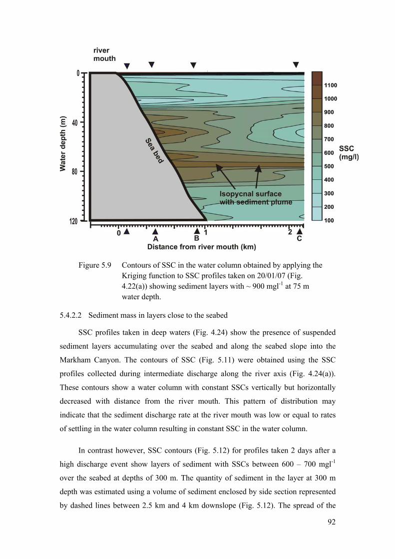
Figure 5.9 Contours of SSC in the water column obtained by applying the Kriging function to SSC profiles taken on 20/01/07 (Fig. 4.22(a)) showing sediment layers with ~ 900 mgl-1 at 75 m water depth.
5.4.2.2 Sediment mass in layers close to the seabed
SSC profiles taken in deep waters (Fig. 4.24) show the presence of suspended
sediment layers accumulating over the seabed and along the seabed slope into the
Markham Canyon. The contours of SSC (Fig. 5.11) were obtained using the SSC
profiles collected during intermediate discharge along the river axis (Fig. 4.24(a)).
These contours show a water column with constant SSCs vertically but horizontally
decreased with distance from the river mouth. This pattern of distribution may
indicate that the sediment discharge rate at the river mouth was low or equal to rates
of settling in the water column resulting in constant SSC in the water column.
In contrast however, SSC contours (Fig. 5.12) for profiles taken 2 days after a
high discharge event show layers of sediment with SSCs between 600 – 700 mgl-1
over the seabed at depths of 300 m. The quantity of sediment in the layer at 300 m
depth was estimated using a volume of sediment enclosed by side section represented
by dashed lines between 2.5 km and 4 km downslope (Fig. 5.12). The spread of the
92
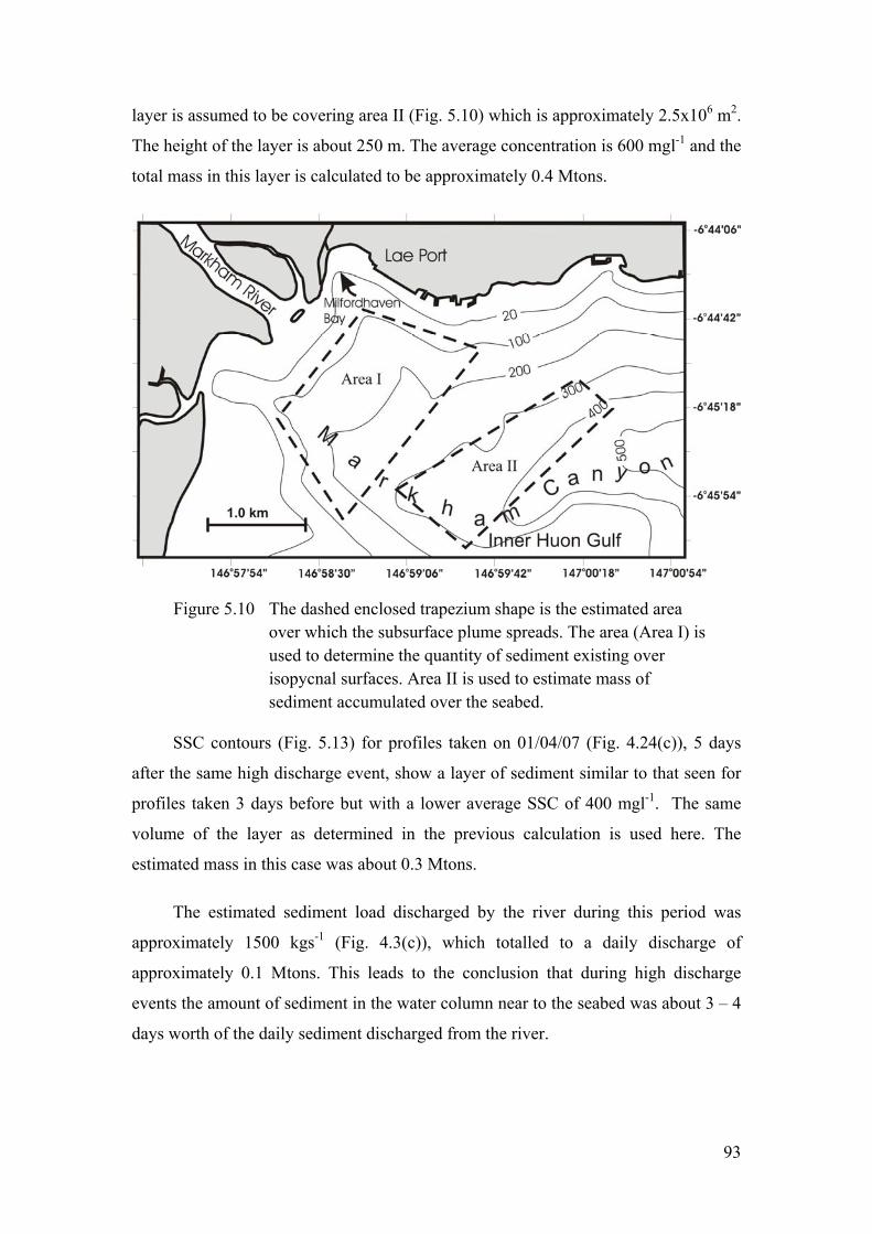
layer is assumed to be covering area II (Fig. 5.10) which is approximately 2.5x10⁶ m2.
The height of the layer is about 250 m. The average concentration is 600 mgl-1 and the
total mass in this layer is calculated to be approximately 0.4 Mtons.
Figure 5.10 a is
ine the quantity of sediment existing over isopycnal surfaces. Area II is used to estimate mass of
bed.
e of
approximately 0.1 Mtons. This leads to the conclusion that during high discharge
event
The dashed enclosed trapezium shape is the estimated areover which the subsurface plume spreads. The area (Area I)used to determ
sediment accumulated over the sea
SSC contours (Fig. 5.13) for profiles taken on 01/04/07 (Fig. 4.24(c)), 5 days
after the same high discharge event, show a layer of sediment similar to that seen for
profiles taken 3 days before but with a lower average SSC of 400 mgl-1. The same
volume of the layer as determined in the previous calculation is used here. The
estimated mass in this case was about 0.3 Mtons.
The estimated sediment load discharged by the river during this period was
approximately 1500 kgs-1 (Fig. 4.3(c)), which totalled to a daily discharg
s the amount of sediment in the water column near to the seabed was about 3 – 4
days worth of the daily sediment discharged from the river.
93
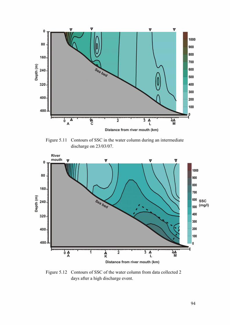
Figure 5.11 Contours of SSC in the water column during an intermediate discharge on 23/03/07.
Figure 5.12 Contours of SSC of the water column from data collected 2 days after a high discharge event.
94
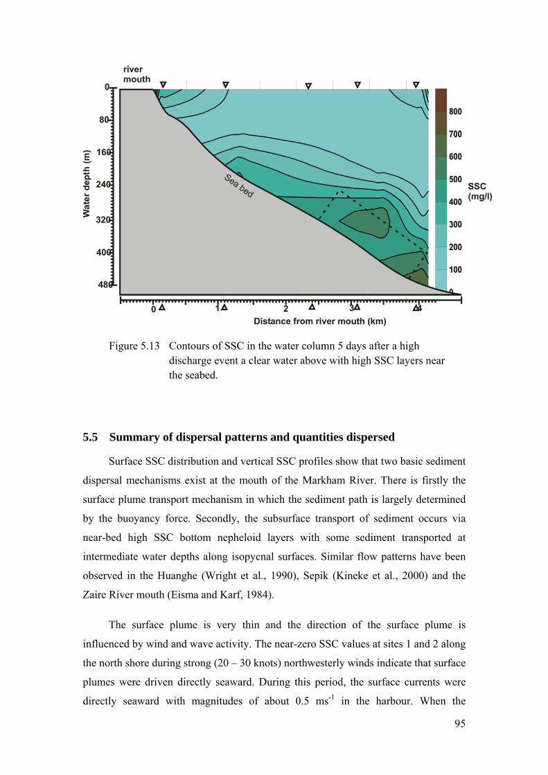
Figure 5.13 discharge event a clear water above with high SSC layers near the seabed.
5.5 Summary of dispersal patterns and quantities dispersed
Surface SSC distribution and vertical SSC profiles show that two basic sediment
dispersal mechanisms exist at the mouth of the Markham River. There is firstly the
surface plume transport mechanism in which the sediment path is largely determined
by the buoyancy force. Secondly, the subsurface transport of sediment occurs via
near-bed high SSC bottom nepheloid layers with some sediment transported at
intermediate water depths along isopycnal surfaces. Similar flow patterns have been
observed in the Huanghe (Wright et al., 1990), Sepik (Kineke et al., 2000) and the
Zaire River mouth (Eisma and Karf, 1984).
The surface plume is very thin and the direction of the surface plume is
influe along
the north shore dur terly winds indicate that surface
plumes were driven directly seaward. During this period, the surface currents were
directly seaward with magnitudes of about 0.5 ms-1 in the harbour. When the
Contours of SSC in the water column 5 days after a high
nced by wind and wave activity. The near-zero SSC values at sites 1 and 2
ing strong (20 – 30 knots) northwes
95
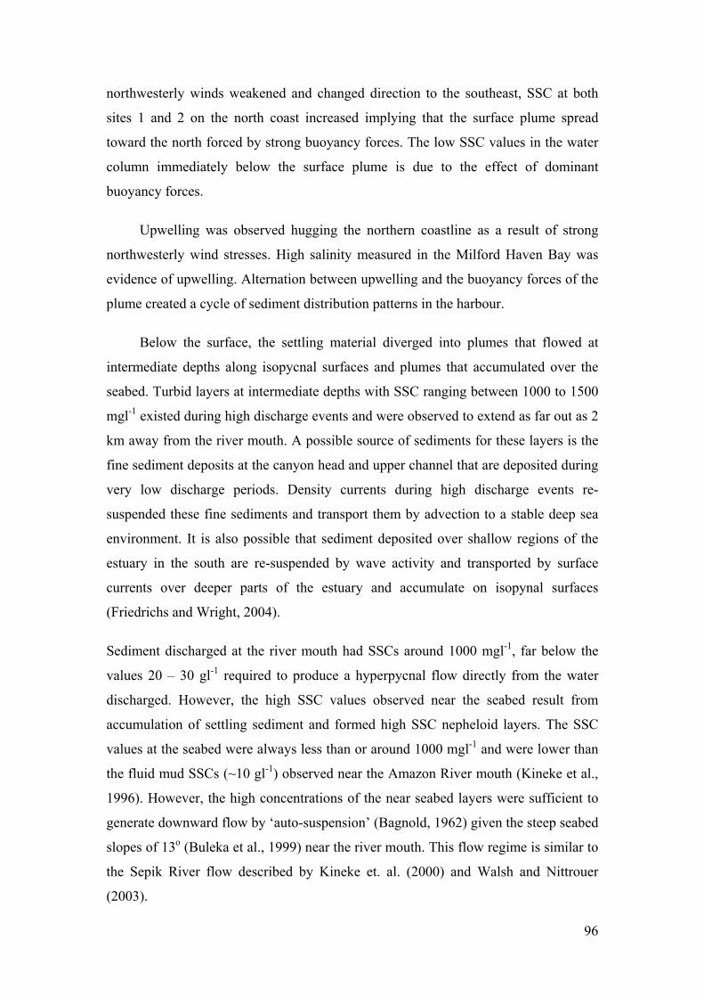
northwesterly winds weakened and changed direction to the southeast, SSC at both
sites 1 and 2 on the north coast increased implying that the surface plume spread
toward the north forced by strong buoyancy forces. The low SSC values in the water
column immediately below the surface plume is due to the effect of dominant
buoyancy forces.
Upwelling was observed hugging the northern coastline as a result of strong
northwesterly wind stresses. High salinity measured in the Milford Haven Bay was
evidence of upwelling. Alternation between upwelling and the buoyancy forces of the
plume created a cycle of sediment distribution patterns in the harbour.
Below the surface, the settling material diverged into plumes that flowed at
intermediate depths along isopycnal surfaces and plumes that accumulated over the
seabed. Turbid layers at intermediate depths with SSC ranging between 1000 to 1500
mgl-1 existed during high discharge events and were observed to extend as far out as 2
km aw ers is the
fine sediment depo ing
very low discharge periods. Density currents during high discharge events re-
suspended these fine sediments and transport them by advection to a stable deep sea
environment. It is also possible that sediment deposited over shallow regions of the
ted by surface
curre
the Amazon River mouth (Kineke et al.,
1996)
ay from the river mouth. A possible source of sediments for these lay
sits at the canyon head and upper channel that are deposited dur
estuary in the south are re-suspended by wave activity and transpor
nts over deeper parts of the estuary and accumulate on isopynal surfaces
(Friedrichs and Wright, 2004).
Sediment discharged at the river mouth had SSCs around 1000 mgl-1, far below the
values 20 – 30 gl-1 required to produce a hyperpycnal flow directly from the water
discharged. However, the high SSC values observed near the seabed result from
accumulation of settling sediment and formed high SSC nepheloid layers. The SSC
values at the seabed were always less than or around 1000 mgl-1 and were lower than
the fluid mud SSCs (~10 gl-1) observed near
. However, the high concentrations of the near seabed layers were sufficient to
generate downward flow by ‘auto-suspension’ (Bagnold, 1962) given the steep seabed
slopes of 13o (Buleka et al., 1999) near the river mouth. This flow regime is similar to
the Sepik River flow described by Kineke et. al. (2000) and Walsh and Nittrouer
(2003).
96
6 Numerical model of the Markham Estuary
6.1 Introduction
Numerical modeling of the Markham estuary (Fig. 3.1) has never been done
before and has been carried out here to predict the hydrodynamics of the estuary
under
ediment in the
area and its influence on the hazardous nature of the environment and on industrial
, 2008).
, 1990) and North Bay, Florida (Huang, 2007). The performance of the model
varying riverine and meteorological conditions during the wet seasons when the
river discharge varies between 250 – 1200 m3s-1. During this period, there is a daily
cycle of strong northwesterly and southeasterly winds in the Inner Gulf. It is useful to
model the Markham estuary considering the impact of the transported s
developments earmarked for the estuarine shoreline. The Princeton Ocean Model
(POM) is used here for this exercise.
6.2 The POM Model
Numerical models have been widely used in predicting estuarine/ocean
dynamics patterns in the past. A collective approach to model development over time
has increased their efficiency in representing real systems. One such model is the
Princeton Ocean Model (POM) developed by Blumberg and Mellor (1987) and
applied to oceanographic problems in the Atmospheric and Oceanographic Sciences
Department of the Princeton University. This model is available for public use from
the POM website (Oey and Ezer
The POM model is popular in the community for ocean circulation modelling.
The model incorporates reasonably complete physics and reliable (and simple)
numerical algorithms. The model has been verified against observations for a wide
range of model configurations. It is recognized by the oceanographic community that
the model performs well especially in coastal regions. The curvilinear orthogonal
coordinates of the model are quite flexible and allow generation of efficient variable-
resolution grids for regions with complicated coastline.
The model has been used successfully in other estuaries; for example, the
Hudson-Raritan estuary (Oey et al., 1985), Chesapeake Bay (Blumberg and Goodrich,
1990), Delaware Bay (Galperin and Mellor, 1990), New York Bight (Blumberg and
Galperin
97
was assessed by comparison with field data for all these applications indicating
confidence that the model reproduces the physical dynamics of the study areas. The
imulating the estuarine responses to time-dependent wind and
multiple river inputs. Details of model descriptions were discussed by Blumberg and
Mello
horizontal and vertical location determined by
the computational grid. This model incorporates a second-order turbulence closure
dy viscosity and diffusivity for the vertical mixing (Mellor
and Y
curvilinear orthogonal coordinates and an
“Arakawa C” differencing scheme. This scheme offsets grid locations at
model is capable of s
r (1987), and the enhanced version of the curvilinear coordinate formulation is
given by Blumberg and Galperin (1990).
6.2.1 Description of the model
POM is a semi-implicit, finite-difference model that can be used to determine
the temporal and spatial changes of surface elevation, salinity, temperature, and
velocity in response to wind, tide, buoyancy, and Coriolis forces. The model solves a
coupled system of differential, prognostic equations describing conservation of mass,
momentum, heat and salinity at each
sub-model that provides ed
amada, 1982).
The principle attributes of the model are as follows:
o It is a sigma coordinate model in that the vertical coordinate is scaled on
the water column depth.
o The horizontal grid uses
which the u-component of velocity, the v-component of velocity, and the
sea level, temperature and salinity are calculated.
o The horizontal time differencing is explicit where as the vertical
differencing is implicit. The latter eliminates time constraints for the
vertical coordinate and permits the use of fine vertical resolution in the
surface and bottom boundary layers.
o The model has a free surface and a split time step. The external mode
portion of the model is two-dimensional and uses a short time step based
on CFL condition and the external wave speed. The internal mode is
98
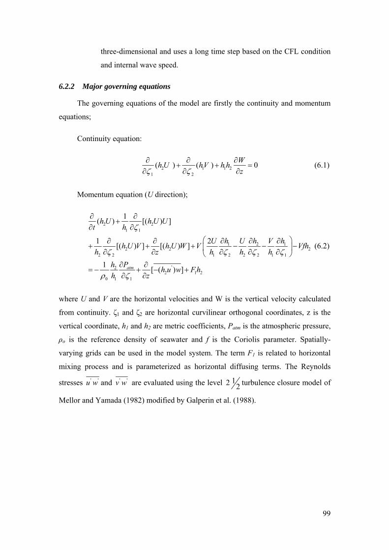
three-dimensional and uses a long time step based on the CFL condition
and internal wave speed.
6.2.2 Major governing equations
The governing equations of the model are firstly the continuity and momentum
equations;
Continuity equation:
2 1 1 21 2
( ) ( ) 0W
h U hV h hz
(6.1)
Momentum equation (U direction);
2 21 1
1 2 12 2
2 2
1( ) [( ) ]
1 2[(
h U h U Ut h
h h hU U Vh U
h
21 2 2 2 1 1
) ] [( ) ]
1
V h U W V Vfhz h h h
Ph
(6.2)
wher
from tal curvilinear orthogonal coordinates, z is the
v
ρo is
vary
mixi terms. The Reynolds
stresses
'22 1 2
0 1 1
[ ( ) ]atm h u w F hh z
e U and V are the horizontal velocities and W is the vertical velocity calculated
continuity. ζ1 and ζ2 are horizon
ertical coordinate, h1 and h2 are metric coefficients, Patm is the atmospheric pressure,
the reference density of seawater and f is the Coriolis parameter. Spatially-
ing grids can be used in the model system. The term F1 is related to horizontal
ng process and is parameterized as horizontal diffusing
' 'u w and ' 'v w are evaluated using the level 1 turbulence closure model of
M
2 2
ellor and Yamada (1982) modified by Galperin et al. (1988).
99
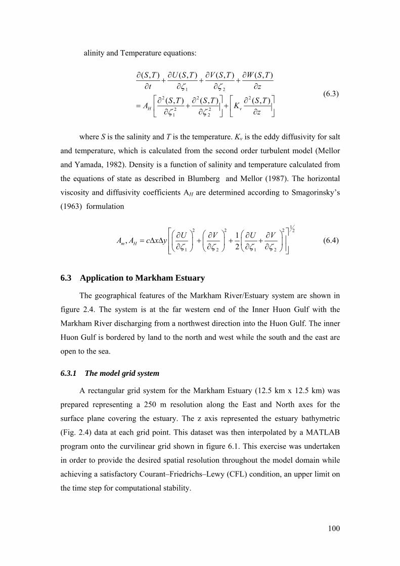
alinity and Temperature equations:
1 2
2 2 2
2 2
( , ) ( , ) ( , )H v
S T S T S TA K
z
1 2
( , ) ( , ) ( , ) ( , )S T U S T V S T W S T
z
t
(6.3)
T is the temperature. Kv is the eddy diffusivity for salt
and temperature, which is calculated from the second order turbulent model (Mellor
and Yamada, 1982). Density is a function of salinity and temp ature calculated
the equations of state as described in Blumberg and Mellor (1987). The horizontal
viscosity and diffusivity coefficients A are determined according to Smagorinsky’s
(1963) formulation
where S is the salinity and
er from
H
12 2 2 2
1 2 1 2
1,
2m H
U V U VA A c x y
(6.4)
6.3 Application to Markham Estuary
The geographical features of the Markham River/Estuary system are shown in
stuar
prepared representing a 250 m resolution along the East and North axes for the
ary bathymetric
(Fig. 2.4) data at each grid point. This dataset was then interpolated by a MATLAB
program onto the curvilinear grid shown in figure 6.1. This exercise was undertaken
in order to provide the desired spatial resolution throughout the model domain while
achieving a satisfactory Courant–Friedrichs–Lewy (CFL) condition, an upper limit on
the time step for computational stability.
figure 2.4. The system is at the far western end of the Inner Huon Gulf with the
Markham River discharging from a northwest direction into the Huon Gulf. The inner
Huon Gulf is bordered by land to the north and west while the south and the east are
open to the sea.
6.3.1 The model grid system
A rectangular grid system for the Markham E y (12.5 km x 12.5 km) was
surface plane covering the estuary. The z axis represented the estu
100
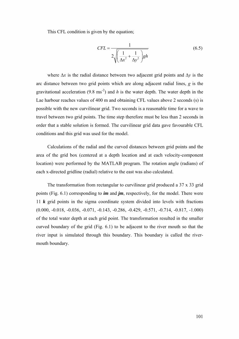
This CFL condition is given by the equation;
2 2
1 12
CFL
ghx y
1 (6.5)
where x is the radial distance between two adjacent grid points and y is the
arc d
formed. The curvilinear grid data gave favourable CFL
conditions and this grid was used for the model.
alculations of the radial and the curved distances between grid p
area of the grid box (centered at a depth location and at each velocity-component
rogram. The rotation angle (radians) of
each x-directed gridline (radial) relative to the east was also calculated.
.036, -0.071, -0.143, -0.286, -0.429, -0.571, -0.714, -0.817, -1.000)
of the total water depth at each grid point. The transformation resulted in the smaller
ig. 6.1) to be adjacent to the river mouth so that the
river
istance between two grid points which are along adjacent radial lines, g is the
gravitational acceleration (9.8 ms-2) and h is the water depth. The water depth in the
Lae harbour reaches values of 400 m and obtaining CFL values above 2 seconds (s) is
possible with the new curvilinear grid. Two seconds is a reasonable time for a wave to
travel between two grid points. The time step therefore must be less than 2 seconds in
order that a stable solution is
C oints and the
location) were performed by the MATLAB p
The transformation from rectangular to curvilinear grid produced a 37 x 33 grid
points (Fig. 6.1) corresponding to im and jm, respectively, for the model. There were
11 k grid points in the sigma coordinate system divided into levels with fractions
(0.000, -0.018, -0
curved boundary of the grid (F
input is simulated through this boundary. This boundary is called the river-
mouth boundary.
101
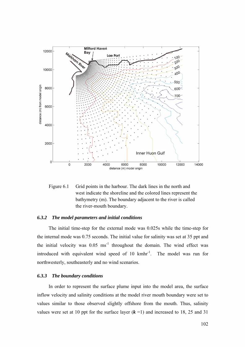
Figure 6.1 Grid points in the harbour. The dark lines in the north and west indicate the shoreline and the colored lines represent the bathymetry (m). The boundary adjacent to the river is called the river-mouth boundary.
6.3.2 The model parameters and initial conditions
The initial time-step for the external mode was 0.025s while the time-step for
the internal mode was 0.75 seconds. The initial value for salinity was set at 35 ppt and
the initial velocity wa -1s 0.05 ms throughout the domain. The wind effect was
introduced with equivalent wind speed of 10 kmhr-1. The model was run for
northwesterly, southeasterly and no wind scenarios.
6.3.3 The boundary conditions
In order to represent the surface plume input into the model area, the surface
inflow velocity and salinity conditions at the model river mouth boundary were set to
values similar to those observed slightly offshore from the mouth. Thus, salinity
values were set at 10 ppt for the surface layer (k =1) and increased to 18, 25 and 31
102
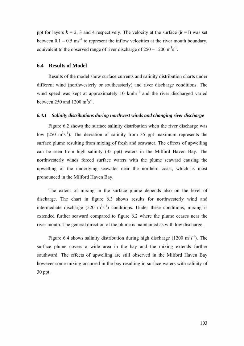
ppt for layers k = 2, 3 and 4 respectively. The velocity at the surface (k =1) was set
between 0.1 – 0.5 ms-1 to represent the inflow velocities at the river mouth boundary,
equivalent to the observed range of river discharge of 250 – 1200 m3s-1.
6.4 Results of Model
Results of the model show surface currents and salinity distribution charts under
different wind (northwesterly or southeasterly) and river discharge conditions. The
wind speed was kept at approximately 10 kmhr-1 and the river discharged varied
between 250 and 1200 m3s-1.
6.4.1 Salinity distributions during northwest winds and changing river discharge
Figure 6.2 shows the surface salinity distribution when the river discharge was
low (250 m3s-1). The deviation of salinity from 35 ppt maximum represents the
surface plume resulting from mixing of fresh and seawater. The effects of upwelling
can be seen from high salinity (35 ppt) waters in the Milford Haven Bay. The
northwesterly winds forced surface waters with the plume seaward causing the
upwelling of the underlying seawater near the northern coast, which is most
pronounced in the Milford Haven Bay.
The extent o l of
discharge. The ch and
intermediate disch s. Under these conditions, mixing is
ere the plume ceases near the
river
n surface waters with salinity of
f mixing in the surface plume depends also on the leve
art in figure 6.3 shows results for northwesterly wind
arge (520 m3s-1) condition
extended further seaward compared to figure 6.2 wh
mouth. The general direction of the plume is maintained as with low discharge.
Figure 6.4 shows salinity distribution during high discharge (1200 m3s-1). The
surface plume covers a wide area in the bay and the mixing extends further
southward. The effects of upwelling are still observed in the Milford Haven Bay
however some mixing occurred in the bay resulting i
30 ppt.
103
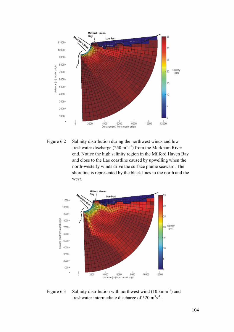
Figure 6.2 Salinity distribution during the northwest winds and low freshwater discharge (250 m3s-1) from the Markham River end. Notice the high salinity region in the Milford Haven Bay and close to the Lae coastline caused by upwelling when the north-westerly winds drive the surface plumshoreline is represent
e seaward. The ed by the black lines to the north and the
west.
Figure 6.3 Salinity distribution with northwest wind (10 kmhr-1) and freshwater intermediate discharge of 520 m3s-1.
104
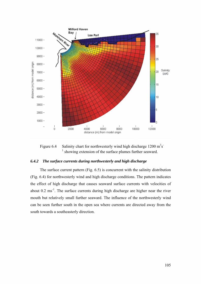
Figure 6.4 ing extension of the surface plumes further seaward.
6.4.2 The surface currents during northwesterly and high discharge
The surface current pattern (Fig. 6.5) is concurrent with the salinity distribution
(Fig. 6.4) for northwesterly wind and high discharge conditions. The pattern indicates
the effect of high discharge that causes seaward surface currents with velocities of
about 0.2 ms-1. The surface currents during high discharge are higher near the river
mouth but relatively small further seaward. The influence of the northwesterly wind
can be seen further south in the open sea where currents are directed away from the
south towards a southeasterly direction.
Salinity chart for northwesterly wind high discharge 1200 m3s-
1 show
105
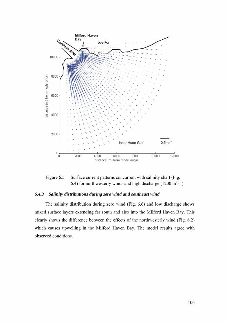
Figure 6.5 Surface current patterns concurrent with salinity chart (Fig. m3s-1).
6.4.3
6.4) for northwesterly winds and high discharge (1200
Salinity distributions during zero wind and southeast wind
The salinity distribution during zero wind (Fig. 6.6) and low discharge shows
mixed surface layers extending far south and also into the Milford Haven Bay. This
clearly shows the difference between the effects of the northwesterly wind (Fig. 6.2)
which causes upwelling in the Milford Haven Bay. The model results agree with
observed conditions.
106
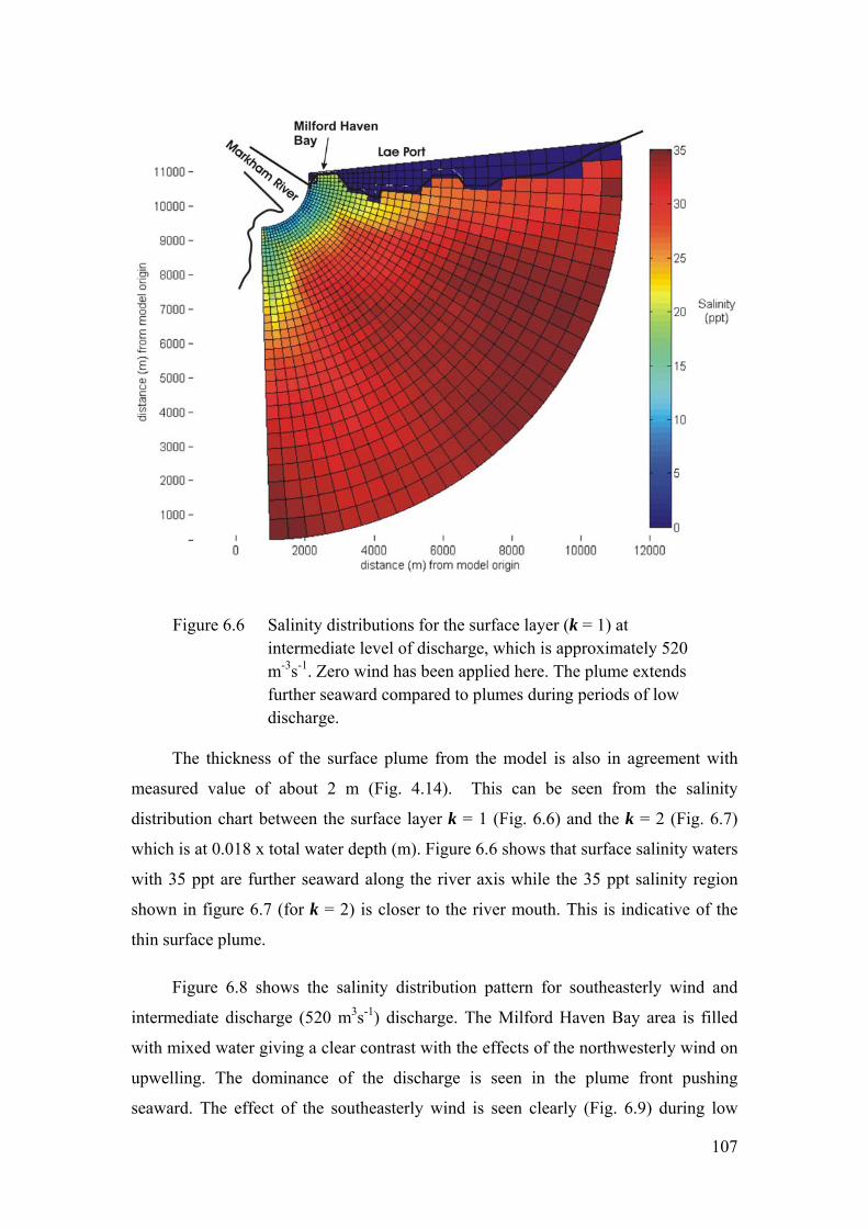
Figure 6.6 Salinity distributions for the surface layer (k = 1) at intermediate level of discharge, which is approximately 520
discharge.
The thickness of the surface plume from the model is also in agreement with
shown in figure 6.7 (for k = 2) is closer to the river mouth. This is indicative of the
thin surface plume.
Figure 6.8 shows the salinity distribution pattern for southeasterly wind and
intermediate discharge (520 m3s-1) discharge. The Milford Haven Bay area is filled
with mixed water giving a clear contrast with the effects of the northwesterly wind on
upwelling. The dominance of the discharge is seen in the plume front pushing
seaward. The effect of the southeasterly wind is seen clearly (Fig. 6.9) during low
m-3s-1. Zero wind has been applied here. The plume extends further seaward compared to plumes during periods of low
measured value of about 2 m (Fig. 4.14). This can be seen from the salinity
distribution chart between the surface layer k = 1 (Fig. 6.6) and the k = 2 (Fig. 6.7)
which is at 0.018 x total water depth (m). Figure 6.6 shows that surface salinity waters
with 35 ppt are further seaward along the river axis while the 35 ppt salinity region
107
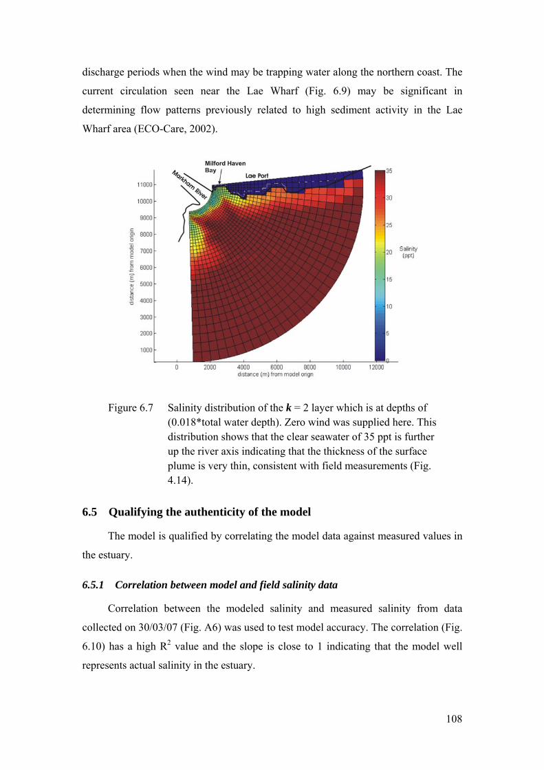
discharge periods when the wind may be trapping water along the northern coast. The
current circulation seen near the Lae Wharf (Fig. 6.9) may be significant in
determining flow patterns previously related to high sediment activity in the Lae
Wharf area (ECO-Care, 2002).
Figure 6.7
r axis indicating that the thickness of the surface
etween model and field salinity data
Correlation between the modeled salinity and measured salinity from data
collected on
Salinity distribution of the k = 2 layer which is at depths of (0.018*total water depth). Zero wind was supplied here. Thisdistribution shows that the clear seawater of 35 ppt is furtheup the riverplume is very thin, consistent with field measurements (Fig. 4.14).
6.5 Qualifying the authenticity of the model
The model is qualified by correlating the model data against measured values in
the estuary.
6.5.1 Correlation b
30/03/07 (Fig. A6) was used to test model accuracy. The correlation (Fig.
6.10) has a high R2 value and the slope is close to 1 indicating that the model well
represents actual salinity in the estuary.
108
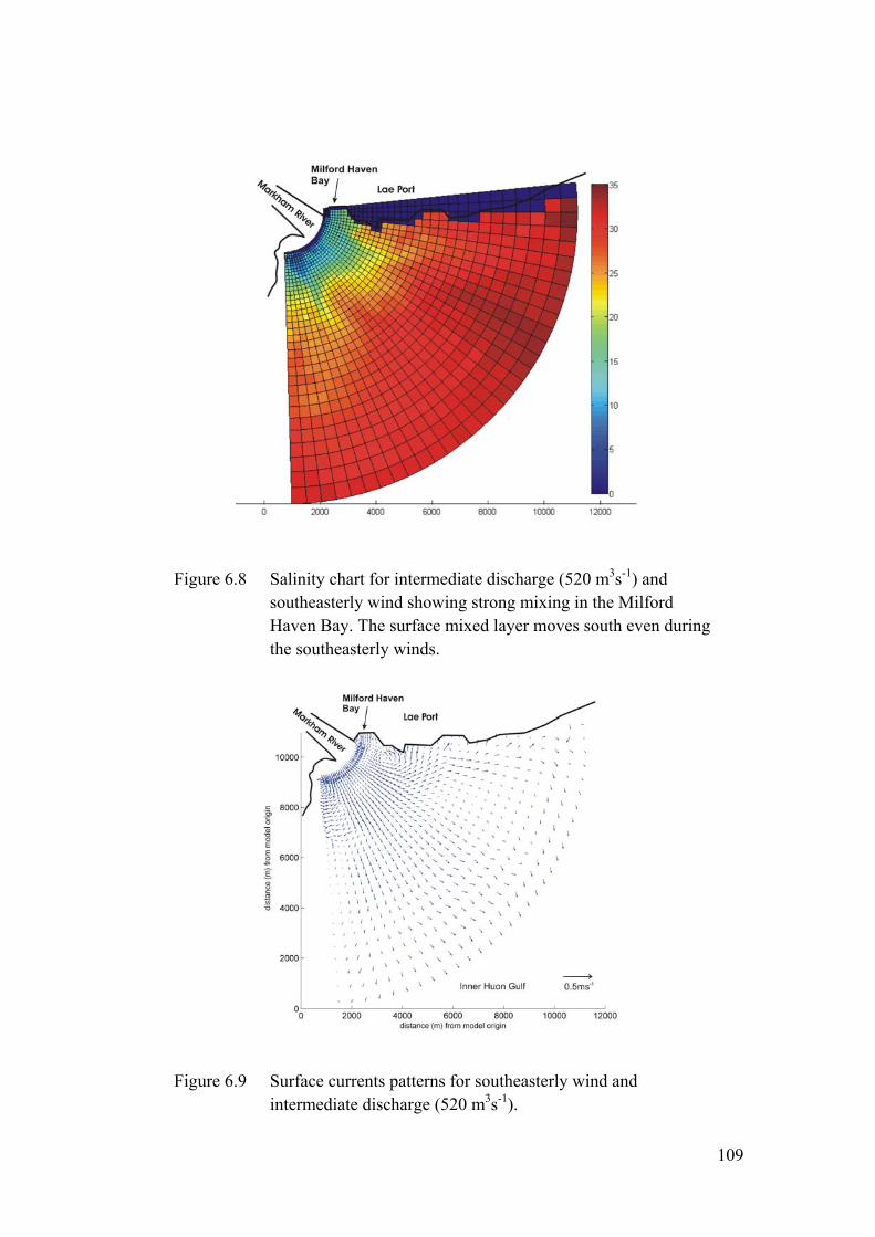
Figure 6.8 Salinity chart for intermediate discharge (520 m3s-1) and southeasterly wind showing strong mixing in the Milford Haven Bay. The surface mixed layer moves south even during the southeasterly winds.
Figure 6.9 Surface currents patterns for southeasterly wind and intermediate discharge (520 m3s-1).
109
Figure 6.10 Correlation between measured surface salinity on 30/03/07 (Fig. A6) and model salinity distribution (Fig. 6.8) for southeasterly wind and intermediate discharge. Conditions of discharge and wind effects applied to model were similar to actual conditions on 30/03/07.
6.5.2 lues
The thicknes for
the top four k laye rder to achieve this estimate, the salinity
values at the k1 layer were corrected at grid points along the river axis. The correction
was done on the basis that the model results given for the top layer were actually the
average value of the model estimates between the top k layer and the next k layer
down. It was necessary to determine the corrected surface (k1 layer) values because of
the large difference in depth between each k layer imposed on the model by the wide
ranging depths in the estuary (up to 500 m depth) and the use of the sigma coordinate
system.
The corrections involved taking the salinity value at k1 and treating it as the
average value of salinity at mid-depth between k1 and k2 layers. The difference in the
two salinity values was then subtracted from the new mid-layer average to give the
corrected salinity value at k1 layer. Corrected salinity values for the top four k layers
were determined for selected grid points along the river axis and plotted on the
appropriate locations on the water depth verses grid points distance axis shown in
figure al shown (Fig.
6.11). This graph shows a salin lumn
Comparing the model surface plume thickness against measured va
s of the surface plume was estimated from model salinity data
rs k1, k2, k3 and k4. In o
6.11. Isoh ine surfaces were estimated from these plots and are
ity structure in the upper surface of the water co
110
which is in reasonable agreement with measured data, shown in (Fig. 4.14(d)-(f)),
taken at sites A, B and C (Fig. 3.3) along the river axis.
Plots of the raw model surface salinity and measured data taken at selected grid
points along the river axis are compared in figure 6.12(a). The disparity between the
model values and the measured values arise from the fact that the model values at the
surface are average values estimated between k1 and k2 layers. The corrected values
for the surface are determined by treating the surface values as the average value
between the two k layers and taking the difference of the two values from the average
value. Figure 6.12(b) show comparisons of the corrected model and measured surface
salinity values which are in agreement indicating again that model is simulating the
estuar
y to a good degree of accuracy.
Figure 6.11 Isohalines of the surface plumes prepared from model data plotted for k layers up to 4 m depth with radial distance from the river mouth. It can be seen that further than 2000 m from the mouth boundary, the thickness of the plume is greater than the thickness of the top model layer.
The good correlation between model and measured salinity data and the
reasonable agreement of plume thickness qualifies the model to be used for modeling
the estuary under varying conditions.
111
Figure 6.12 Comparing salinity data with distance from the river mouth (a) for raw model surface results against measured salinity at sites along the river axis. The raw data are higher than the measured data. (b) corrected model surface salinity determined by taking the salinity at k =1 layer as the average value between k = 1 and 2 and taking the difference of two values from the average value.
6.6 Other applications of the model
arbour
resulting from the m)
(Fig.6.13) that will are
presented and discu lied to the study of sediment
dispersal patterns influenced by the changing river mouth features (Fig. 2.5) resulting
from changing weather patterns (e.g. the eff
The model has been applied to predict current patterns in the Lae H
development of the new tidal basin (700 m x 400 m x 14
be constructed adjoining the Milford Haven Bay. The results
ssed here. This model can also be app
ect of El Nino). Impacts of these changes
will be discussed briefly however the modeling will be left for future studies.
112
113
Figure 6.13 The plan area of the tidal basin (700 m x 400 m x 14 m depth) sketched over a Google Earth photo of Lae Harbour. The area will be dredged to 14 m depth and the waste will be pumped and dumped at 25 m depth 500 m from the river mouth.
6.6.1 Results of current patterns predicted for the tidal basin
The results of the current patterns for intermediate discharge (520 m3s-1) and
southeasterly wind (10 kmhr-1) conditions show that surface currents are directed
inwardly into the tidal basin (Fig. 6.14). Turbid plumes discharged from the river will
be transporting sediment into the basin. Below the surface, at k4 depth (0.071of water
depth), the current (Fig. 6.15) is directed out of the basin along the western edge of
the basin. The out-flowing currents are expected at that depth so that volume is
conserved.
Currents patterns during northwesterly winds and intermediate discharge
conditions show surface currents (Fig. 6.16) directed seaward outside of the Milford
Haven Bay while there is very little flow occurring in the tidal basin.
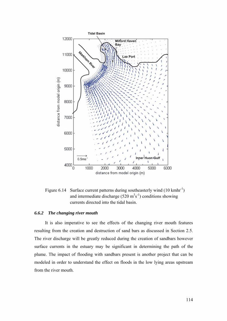
Figure 6.14 Surface current patterns during southeasterly wind (10 kmhr-1)
may be significant in determining the path of the
plum
and intermediate discharge (520 m3s-1) conditions showing currents directed into the tidal basin.
6.6.2 The changing river mouth
It is also imperative to see the effects of the changing river mouth features
resulting from the creation and destruction of sand bars as discussed in Section 2.5.
The river discharge will be greatly reduced during the creation of sandbars however
surface currents in the estuary
e. The impact of flooding with sandbars present is another project that can be
modeled in order to understand the effect on floods in the low lying areas upstream
from the river mouth.
114
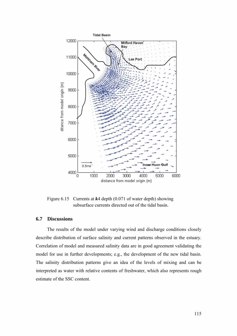
Figure 6.15 Currents at k4 depth (0.071 of water depth) showing subsurface currents directed out of the tidal basin.
6.7 Discussions
The results of the model under varying wind and discharge conditions closely
describe distribution of surface salinity and current patterns observed in the estuary.
Correlation of model and measured salinity data are in good agreement validating the
model for use in further developments; e.g., the development of the new tidal basin.
The salinity distribution patterns give an idea of the levels of mixing and can be
interpreted as water with relative contents of freshwater, which also represents rough
estimate of the SSC content.
115
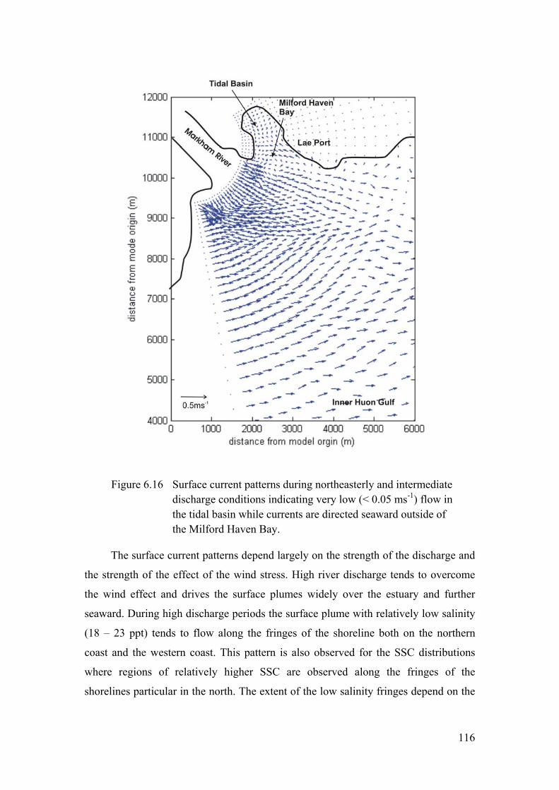
Figure 6.16 termediate discharge conditions indicating very low (< 0.05 ms-1) flow in
e tidal basin while currents are directed seaward outside of the Milford Haven Bay.
his pattern is also observed for the SSC distributions
where regions of relatively higher SSC are observed along the fringes of the
shorelines particular in the north. The extent of the low salinity fringes depend on the
Surface current patterns during northeasterly and in
th
The surface current patterns depend largely on the strength of the discharge and
the strength of the effect of the wind stress. High river discharge tends to overcome
the wind effect and drives the surface plumes widely over the estuary and further
seaward. During high discharge periods the surface plume with relatively low salinity
(18 – 23 ppt) tends to flow along the fringes of the shoreline both on the northern
coast and the western coast. T
116
level of discharge. During low to intermediate discharge the dispersal is wide but
confined to the within 2 kilometres of the river mouth.
During strong northwesterly winds and low to intermediate discharge, the
surface plume is driven directly seaward and confined to the open sea direction. This
leaves high salinity seawater along the fringes of the coastline. The edge of the
surface plumes then spread northward or westward under the influence of strong
buoyancy forces when the wind velocity subsides. The seaward flow of the surface
waters during strong northwesterly winds create upwelling at the fringes of the
northern coastline where undiluted seawater is observed (e.g., Milford Haven Bay).
During these conditions, the surface waters are driven seaward and the underlying
seawater rises to the surface along the northern coast so that volumes are conserved.
117
7 Instrumentation for measuring suspended sediment concentration (SSC)
The third part of this project was aimed at designing an instrument that is able to
measure time-series of suspended sediment concentration without using optical
methodologies and also to simultaneously provide information on settling velocities.
The primary motivation of the work was to find a method to overcome the calibration
difficulties that occur using optical instruments for determining SSC.
7.1 Introduction
Calibration of optical instruments can vary by up to an order of magnitude with
changes in particle size (Renagi, 2000). Typically large particle sizes scatter light less
an small particles for the same sediment concentration. Because of this particle size
variation, site-specific calibrations to produce SSC must be carried-out. This is often
done with sediment samples taken from the seabed and raises the question of whether
these are representative of the material in suspension. Further, particle size
distributions can change with time and physical condition. For example during
periods of wave resuspension, it is possible that a coarser fraction of sediment is in
suspension, and thus different calibration coefficients should be used for different
conditions. In practice this is never done.
The initial intention was to use the equipment for the study of the Markham
River, however it was evident that this was not possible given time constraints.
Instead the instrumentation work became more of a scoping study to prove the
principle of operation for further work in the future.
In this work a differential pressure sensor is used to determine the SSC.
Although the use of differential sensors is not new for this application, a new
approach to removing common mode errors is proposed and investigated. In essence
the method uses two measurements of differential pressure in a water column, one
before the sediment has settled from the column, and one after it has settled. The
difference in the readings is used to determine SSC. In order to reduce common mode
errors and temporal drift in the sensor, the readings are referenced against a standard
th
118
pressure difference. In essence there are three pressure difference measuremen
thus we have termed this technique
ts and
a triple differential pressure technique.
Many different instruments and techniques have been developed to measure
SSC
et al., 1996) or
laser beams e.g. (Agrawal and Pottsmith, 2000; Bale, 1996) mounted at selected
n. The backscatter or transmit intensity of the sensors are
calibr
r, 1995) and changes in the natural setting
when removing samples from the environment to the laboratory for calibration
purpo
acoustic backscatter systems are
comm
in density is measured as the sediment settles in a water column.
in marine studies to quantify the settling flux in-situ. For example, Eisma et.
al.,(1997) Jones and Jago (1996) and Pejrup and Edelvang (1996) developed and used
settling tubes in which sub-samples were withdrawn from the tube at selected time
interval and SSC values determined in the laboratories using gravimetric methods.
Advanced techniques include the use of optical sensors e.g. (Murray
heights in a settling colum
ated against measured SSC to determine times series SSC in the settling
columns. Modern equipment use non-intrusive, holographic (Carder et al., 1982;
Costello et al., 1989) and acoustic backscatter techniques (Fugate and Friedricks,
2002).
The accuracy of the SSC measurements vary between methods and instruments
used. The use of settling columns in various environments has given approximately
82% variance in concentration values when calculating settling parameters (Pejrup
and Edelvang, 1996). Factors contributing to this large variance includes the temporal
change in characteristics of particles (Dye
ses. Optical devises have been used to determine in-situ SSC, however errors of
30% (Larcombe et al., 1995) has been observed due to the influence of a number of
particle characteristics to backscatter signal (Hatcher et al., 2000; Renagi, 2000;
Sutherland et al., 2000). Holographic techniques and
on and relatively accurate but expensive.
7.2 The Principle of Design
The principle of measurement is based on the fact that when sediment settles out
of a water column, the density of the fluid changes. A differential pressure sensor can
be used to directly measure the density of the water, however the water density also
depends upon other factors such as temperature and salinity. In this work the change
119

A schematic diagram of the instrument design is shown in figure 7.1 and details
will be given in the next section. In this section however, the principle behind the
design will be discussed with reference to the dimensions given in the diagram. The
two points between which the differential pressure is measured is top port (Pt) and the
bottom port (Pb) of the pressure sensor. The following equations describe the
interpretation of the measured data.
The pressure at top port;
1 2t w oP gh gh (7.1)
while pressure at the bottom port is;
3 4b w oP gh gh (7.2)
The terms and are the densities of water and oil respectively. The
component of water and oil in the conn
w o
ecting tubes and the meniscus control
chambers are shown in figure 7.1. The corresponding heights (h1, h2, h3 and h4) for
corresponding fluid type with respect to reference points of sensing of pressure are
also shown in the figure 7.1. The differential pressure (PT-PB) is given by taking
equation 7.2 from 7.1;
1 2 3 4T B w o w oP P h g h g h g h g (7.3)
Rearranging
1 3 )T B w 2 4( ) (oP P g h h g h h (7.4)
But, h h h h h where h is the height difference between the two
r sections. Substituting term in the above equation
7.4 gi
2 4 1 3
menisci between the oil and wate
ves;
T B w oP P gh gh (7.5)
Rearranging
120
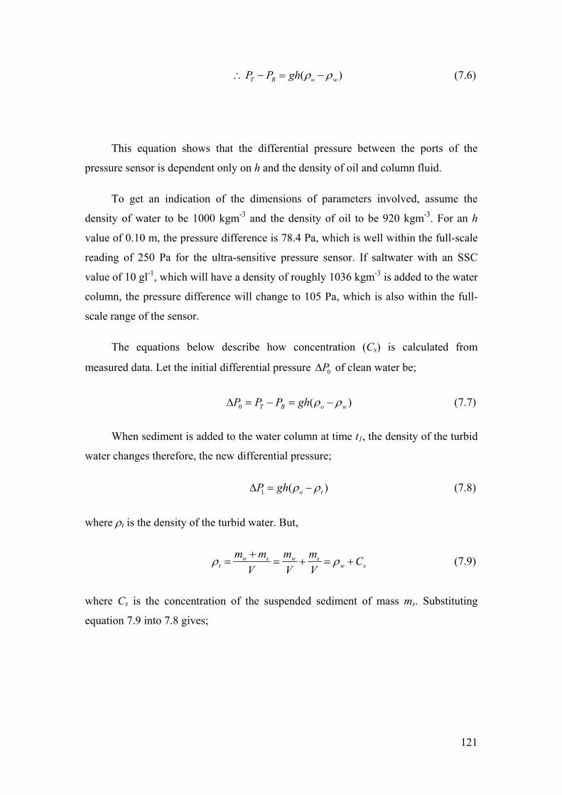
( )T B o wP P gh (7.6)
This equation shows that the differential pressure between the ports of the
pressure sensor is dependent only on h and the density of oil and column fluid.
the dimensions of parameters involved, assume the
density of water to be 1000 kgm-3 and the density of oil to be 920 kgm-3. For an h
value of 0.10 m, the pressure difference is 78.4 Pa, w
reading of 250 Pa for the ultra-sensitive pressure sensor. If saltwater with an SSC -3 is added to the water
colum , the pressure difference will change to 105 P
scale range of the sensor.
To get an indication of
hich is well within the full-scale
value of 10 gl-1, which will have a density of roughly 1036 kgm
n a, which is also within the full-
The equations below describe how concentration (Cs) is calculated from
measured data. Let the initial differential pressure 0P of clean water be;
0 ( )T B o wP P P gh (7.7)
When sediment is added to the water column at time t1, the density of the turbid
water c e new differential pressure;
( )P gh
hanges therefore, th
1 o t (7.8)
e density of the turbid water. But,
where t is th
w s w st w C
V V V s
m m m m (7.9)
where C is the concentration of the suspended sediment of mass m . Substituting s s
equation 7.9 into 7.8 gives;
121
1 0 sP P ghC (7.10)
The change in the differential pressure is therefore;
1 0( ) sP P P ghC (7.11)
This equation clearly shows that (P) is a direct measure of depth-average
suspe
7.3 Instrument
erentia to measure
minute changes in the hydrostatic pressure caused by
suspended particles in the water column. The design comes in three parts; the water
colum
he water column was 30 cm high and had a 10
had a top and bottom outlets 2.5 cm from each end of the column. The outlets were
cus control (MC) chambers by 4 mm
plastic tubing as shown in the diagram. The top ends of the MC chambers were
onnected to the pressure sensor as shown in the diagram. Th
perspex tubing of 5 cm inner diameter and 6cm in height.
filled with water and the MC chambers were positioned
such that the water levels in the chambers where about even. The tubes leading out of
the two chambers were filled with olive oil until filled. The two outlets of the
differential pressure sensor were then inserted into the overflowing ends of the tube
leading out of the chamber. Care was taken to avoid air bubbles being trapped in the
nded sediment concentration in the water column. By measuring the P with the
sediment in suspension, and some time later when the sediment has settled out of the
tube, a measure of the SSC can be made that does not depend upon the density of the
water. To this stage there are two differencing operations involved. As mentioned
above, the pressure sensor can be periodically switched to a reference pressure
difference to reduce temporal drift and common mode errors.
The schematic diagram of the prototype instrument is shown in figure 7.1
below. The instrument uses an ultra-sensitive diff l pressure sensor
the introduction or loss of
n, measurement control system, which includes the valve and meniscus control
chambers and the ultrasensitive pressure sensor.
T cm inner diameter. The column
connected to the lower outlets of the two menis
c e chambers are made of
The water column was
122
sensor ports. The two chambers were placed side
(approximately 10 mm) between the two meniscus levels.
by side with some distance h
Figure 7.1 Design of the system with a differential pressure sensor to measure small changes in pressure as sediment falls in enclosed water column.
by tension forces between the liquid and the tube wall. The purpose of the oil is to
The purpose of the meniscus control chamber is to reduce the movement of
menisci levels during the operation of the manual valves and the pressure changes
when sediment is added to the water column. The larger radius of the chamber also
reduces the pressure difference across the interface due to the capillary effect created
123
protect the diaphragms of the pressure sensor from water. However, it is important
that the density of oil be close to that of water so that the desired range of differential
pressure is within the full-scale response of the sensor, which is ± 1 inch of H2O or
50 kPa.
Common mode errors and sensor drift were corrected using a third differencing
operation using two valves to switch the pressure sensor to a constant pressure
difference. The two valves, VA and VB (Fig. 7.1) are operated manually in the
prototype system. When VA was closed and VB was kept open the sensor read the
differential pressure at the top surface of the water column. This pressure is called the
surface differential pressure (SDP) and is effectively a “zero” reading. With valves in
the opposite position (VA open and VB closed) the sensor reads the differential
pressure in the water column which is called the column differential pressure (CDP).
The specifications of the differential pressure sensor are given in Appendix 2.
The pressure sensor voltage output leads were connected to a programmable data
logging system similar to those used in the Optical Backscatter sensors so that time
series SSC can be recorded.
7.4 Methods
In order to determine the sensitivity of the method, an experiment was carried
out to record the sensor output voltage for the SDP and the CDP for varying water
densities. Water density was varied by adding 0.4 g of salt to the column. It should be
noted that for this experimental set-up, salt was used instead of sediment to vary
density. This was done because there are no issues with sediment settling, and this
ity analysis rather than a test of a functioning sy tem. The
colum iving it
a volume of 456 cm olumn. The
valve was operated m d B open, Pt = Pb and the
press
2
experiment is a sensitiv s
n had an inner diameter of 4.4 cm and an approximate height of 30 cm, g3. The salt solution was stirred to mix evenly in the c
anually such that when A was closed an
ure difference would be zero and the reading given by the pressure sensor would
represent zero pressure. Subsequently B was closed while A was open and the sensor
voltage output was corresponding to the differential pressure in the water column. It
was noted that the height between the two menisci levels did not change.
124
7.5 Results of sensor voltage output against concentration
Figure 7.2 shows the response of the sensor for different concentrations of salt.
The sensor voltage output was measured with a conventional multi-meter fluctuated in
the fifth significant figure but was steady in the fourth significant figure. It was thus
apparent that measurement with a sensitivity of 0.001 V were reliable. The average
slope of the line in figure 7.2 is 0.019V/gl-1 and thus a resolution of 50 mgl-1 could be
achieved for the system.
Figure 7.2 A linear relationship between the pressure sensor output voltage and concentration.
The experiment was rerun with addition of low concentration with the pressure
sensor voltage recorded both manually using a high sensitivity multi-meter and by the
data logging device. The graph in figure 7.3 shows the linear relationship between the
logger raw data and pressure sensor voltage indicating that 1 logger unit corresponds
to 1.2 mV. The equivalent relationship between SSC and raw logger units (Fig. 7.4)
show that 1 logger unit corresponds to 100 mgl-1.
125
Figure 7.3 Graph showing the relationship between the raw logger units the pressure sensor voltage when in response to increasing mass in the water column.
Figure 7.4 Graph showing relationship between raw logger units and concentration for small increments in concentration. 1 logger unit is equal 100mgl-1.
7.6 Discussion
The above results are probably worst case estimates of the sensor sensitivity and
calculations using the sensor written specifications indicate that a factor of 10
improvement in performance may be achievable. For environments with very high
sediment loads, a resolution of between 10 and 100 mgl-1 would be useful, however
for the Markham river application where concentrations peak at around 1000 mgl-1,
126

such a resolution would be marginal. For this reason, work on the prototype was
suspended.
Despite the lack of resolution for the Markham river study, the method shows
considerable promise for future work. A resolution of 10 mgl-1 would be satisfactory
for many applications. In addition, a taller water column would improve the
sensitivity further and it is highly likely that in the near future the resolution of the
differential pressure sensors will improve. Although this system will always be more
cumbersome than optical measurements, it can give absolute measurements of
sediment concentration that is presently difficult to achieve with optical system . s
127
8 Conclusion
8.1
dely
over the estuary. The surface plume is very thin ~(1.6 m) and very little mixing occurs
between the plume and the underlying ambient seawater. The estuary is microtidal
and any influence on the sediment dispersal is insignificant.
The surface plume flows widely over the bay and the distribution pattern is
strongly influenced by the dominant buoyancy force. The rate of discharge can
influence the extent of the area coverage of the plume. However, the surface plume is
also highly affected by strong northwesterly and southeasterly wind activity which are
predominant during the wet season. During strong (15 – 25 kmhr-1) northwesterly
winds the plume is directly forced seaward leaving clear seawater along the fringes of
the northern coast and the western coast. Buoyancy forces again dominate when the
winds subside. During southeasterly winds, the plume is driven towards the northern
coast and creates turbid waters along the fringes of the northern coast.
In the water column, sediment settling out of the turbulent zone and the surface
plume are observed to be accumulating over isopycnal surfaces and over the seabed.
Sediment is advected along isopycnal surfaces as far as the surface is maintained.
Sediment will settle out of this surface where the isopycnal properties cease. Sediment
accumulating over the seabed have higher SSCs (500 – 1000 mgl-1) have thicknesses
of between 100 – 200 m. Of all the SSC profiles taken, the SSC in these layers was
never higher than 1000 mgl-1 indicating that these layers were flowing downslope into
the Markham canyon under the influence of gravity.
Markham estuary
The Markham, a tropical mountainous river, discharges directly onto the ocean,
creating a highly stratified off-shore estuary during the wet season. The sediment
laden river water, discharged at the river mouth, creates a turbulent mixing zone upon
contact with seawater. Entrainment of saltwater into the mixing zone causes
flocculation of particles that fall out of the mixing zone and settle through the water
column. The surface plumes rise above the mixing zone and spreads sediment wi
128
8.2 Sediment dispersal patterns and quantities
It is obvious that three pathways exist for sediment to be dispersed in the
ment is dispersed by surface plumes, by plumes that
exist
of the river mouth while
the re
hly likely that
turbid
The modified POM model applied to the Markham estuary has given reliable
results. Measured plume results are consistent with model salinity contours for the
estuary. The effect of varying discharge from low (250 m3s-1) to high (1200 m3s-1) on
Markham discharge system. Sedi
at intermediate water depths along isopycnal surfaces and along the seabed by
fluid mud flow. The surface plumes deliver sediment to the seabed along the northern
and the western shoreline and to the open sea. The sediment transported along the
isopycnal surfaces are delivered to the seabed slopes in deeper (30 m and beyond)
waters. Sediment transported along the seabed flows downslope and may settle over
the Markham canyon channel where the downslope currents cease.
The total sediment discharged from the Markham River during a high discharge
event is about 1600 kgs-1 which amounts to a daily discharge of 0.14 Mtons. Of this
amount, 80% is lost to subsurface waters within 2km radius
st is transported by surface plume. The mass of sediment in a layer along a
isopycnal surface was 0.03 Mtons which is only about 30% of the daily sediment lost
to the subsurface waters. The mass of sediment in fluid mud layers over the seabed is
between 0.3 and 0.4 Mtons which is equivalent to 3 to 4 days of sediment discharged.
Turbidity currents created by supercharged sediment load with concentrations
beyond 25 gl-1 in the river were not observed during the field trip. However, high SSC
nepheloid layers, formed by sediment accumulating over the steep (1:10) seabed
slopes, flowed downslope under the influence of gravity as turbidity currents.
Although no velocity measurements were taken at deep waters, it is hig
ity currents created by flow of high SSC nepheloid layers can provide enough
stress to resuspend previously deposited fine sediment and transport them further
downslope into the canyon. Some of the fine material may remain in suspension in the
plumes existing between the canyon walls. This pattern of flow is of interest to the
study of sediment transport of mountainous rivers discharging directly into deep sea
which is analogous to process during low stand sea levels.
8.3 The hydrodynamic model for the Markham estuary
129
the extent of the plume dispersal is also comparable between the measured and model
result
The opportunity
also
100 mgl-1 although I had hoped to obtained resolutions of 1 mV = 10 mgl-1. The
speci
s. The effect of the northwesterly winds on the plume dispersal showing
upwelling activity has been well represented by the model as well. Varying wind and
discharge conditions have been well simulated.
This model therefore provides a reliable tool for testing plume distribution
patterns under different discharge and wind conditions. In addition, prediction of
plume distribution can be made when significant changes in the shoreline morphology
are made; e.g. the construction of the new tidal basin in the Milford Haven Bay or the
changing river mouth positions influenced by the El-Nino cycles.
arises to improve the model resolution near the northern coast where the Lae
wharf is situated so that the hydrodynamics contributing to the high siltation rates
experienced at the wharf between 1995 and 2002 may be tested.
8.4 Triple Differential Pressure Sensor for measuring SSC
The instrument designed to measure SSC directly using an ultra sensitive
differential pressure sensor shows promise. The best resolutions obtained was 1 mV =
fications of the sensor however indicate that the sensor is capable of providing
the required resolution. It has an added advantage over the usual optical backscatter
sensors (OBS) in that there is no need for site specific calibration.
The inclusion of a data logger to the system will allow the system to record time
series SSC. In cases where sediment, already in the water column, is settling out of
the tube, time series SSC data can be used to determine flux and hence the settling
velocity of materials. This measurement can be made in any marine environment
including deep seas, estuaries, rivers and lakes.
130
References
Aalto, R., Lauer, J.W. and Dietrich, W.E., 2008. Spatial and temporal dynamics of
sediment accumulation and exchange along Strickland River floodplains
mposition and
behaviour of trace metals in post-oxic sediments of the Gulf of Papua, PNG.
Bale,
effluent at sea. The Columbian
River Estuary and Adjacent Ocean Waters. University of Washington Press,
Seattle, 41-80 pp.
Bates, C.C., 1953. Rational theory of delta formation. American Association of
Petroleum Geology Bulletin, 37: 2119 - 2161.
(Papua New Guinea) over decadal-to-centennial time scales. J. Geophys. Res.,
113: F01S04.
Agrawal, Y.C. and Pottsmith, H.C., 2000. Instruments for particle size and settling
velocity observations in sediment transport. Marine Geology, 168(1-4): 89-
114.
Allen, P.A., 1997. Earth Surface Processes. Blackwell Science, Cambridge.
Alongi, D.M., Boyle, S.G., Tirendi, F. and Morgui, J.A., 1996. Co
Estuarine, Coastal and Shelf Science, 42: 197-212.
Alvarez, L.G. and Jones, S.E., 2002. Factors Influencing Suspended Sediment Flux in
the Upper Gulf of California. Estuarine, Coastal and Shelf Science, 54(4):
747-759.
Bagnold, R.A., 1962. Autosuspension of transported sediment Proceedings of the
Royal Society, London, 256A: 315-319.
A.J., 1996. In-situ laser optical particle sizing. Journal of Sea Research, 36(1-2):
31-36.
Barnes, C.A., Duxbury, A.C. and Morse, B.A. (Editors), 1972. Circulation and
selected properties of the Columbia River
131
Blumberg, A.F. and
New York B
Galperin, B. (Editors), 1990. On the summer circulation in the
ight Coastal and Estuarine Studies, Residual Currents and Long-
Blumb ation
Blumberg, A.F. and Mellor, G.L. (Editors), 1987. A description of a three-
ashington, 1-16 pp.
al
Brunskill, tion of riverine sediment
Buleka, J., Prior, D.B. and Van der Spek, A., 1999. Coastplan Geology and Natural
eological Survey Division,
Department of Mineral Resources, Papua New Guinea (Port Moresby), and
angkok): 134pp.
ments
Chappell, J., 1974. Geology of coral terraces, Huon Peninsula, New Guinea: a study
iety
Chappell, J., 1983. A revised sea-level record for the last 300,000 years from Papua
New Guinea. Search, 4: 99-101.
term Transport, 38. Springer, New York Inc.
erg, A.F. and Goodrich, D.M., 1990. Modeling of wind-induced destartific
in Cheasapeake Bay. Estuaries, 13(3).
dimensional coastal ocean-circulation model Three-dimensional Coastal
Ocean Models. Coastal and Estuarine Sciences, 4. American Geophysical
Union, W
Brunskill, G.J., 2004. New Guinea and its coastal seas, a testable model of wet
tropical coastal processes: an introduction to Project TROPICS. Continent
Shelf Research, 24(19): 2273-2295.
G.J., Woolfe, K.J. and Zagorskis, I., 1995. Distribu
chemistry on the shelf, slope, and rise of the Gulf of Papua. Geo-Marine
Letters, 15: 160-165.
Hazards of Lae City and Surroundings, Papua New Guinea. CCOP
COASTPLAN Case Study Report No.3, G
Committee for Coordinating Geoscience Programmes in East and Southeast
Asia (B
Carder, K.L., Steward, R.G. and Betzer, P.R., 1982. In-situ holographic measure
of sizes and settling rates of oceanic particulates. Journal of Geophysical
Research, 87 (C8): 5681-5685.
of Quaternary tectonic movements and sea-level changes. Geological Soc
of America Bulletin, 85: 555-570.
132
Chappell, J., Ota, Y. and Berryman, K., 1996. Late Quaternary coseismic uplift
history of Huon Peninsula, Papua New Guinea. Quaternary Science Reviews,
15: 7-22.
Coffey and Hollingsworth, 1969 Report on foundation investigations for the proposed
Markham river bridge, Lae, New Guinea, Melbourne.
rticulate
Costello, D.K., Carder, K.L., Betzer, P.R. and Young, R.W., 1989. In-situ holographic
e
96-1605).
elf
Fly River, Gulf of Papua. J. Geophys. Res., 113:
F01S12.
Day, G ional web
s., 113:
Dyer, K.R., 1973. Estuaries: A Physical Introduction. John Wiley and Sons, New
York, 140 pp.
Dyer, K.R., 1995. Sediment transport proce
dimentology of estuaries. Developments in
sedimentology. Elsevier Science B.V, pp. 423-449.
ECO-Care, E.C., 2002. Lae Port Environm
Conomos, T.J. and Gross, M.G. (Editors), 1972. River-ocean suspended pa
matter relations in seawater. The Columbian River Estuary and Adjacent
Ocean Waters. Washington University Press, Seattle, 172-202 pp.
imaging of settling of settling particles: applications of individual particl
dynamics and oceanic flux measurements. Deep Sea Research and
Oceanographic Abstracts, 36 (10)(15
Crockett, J.S., Nittrouer, C.A., Ogston, A.S., Naar, D.F. and Donahue, B.T., 2008.
Morphology and filling of incised submarine valleys on the continental sh
near the mouth of the
., Dietrich, W.E., Rowland, J.C. and Marshall, A., 2008. The deposit
on the floodplain of the Fly River, Papua New Guinea. J. Geophys. Re
F01S02.
sses in estuaries. In: G.M.E. Perillo
(Editor), Geomorphology and se
ental (Siltation) Study. PNGHB 02-02(1),
PNG Harbour Board Limited, Lae.
133
Eisma, D., Dyer, K.R. and Van Leussen, W. (Editors), 1997. The in-situ
determination of the settling velocities of suspended fine-grained sediment - a
review. Cohesive Sediments. John Wiley &Sons Ltd, 17-44 pp.
arch, 17(2-4): 385-411.
gy.
Falmouth, 2005. NXIC CTD USER MANUAL, Falmouth Scientific Inc.
Eisma, D. and Karf, J., 1984. Dispersal of Zaire River suspended matter in the estuary
and the Angola basin. Netherlands Journal of Sea Rese
Everingham, I.B., 1973. A submarine slump and tsunami in the Lae area of Papua
New Guinea, 26 August 1972. 1973/20, Department of Minerals and Ener
http://www.falmouth.com.
ine, I., 1997. Fiobuoy User Manual, Australia.
J.S., Ditmars, J.D. and Ippen, A.T., 1972. Mathe
Fiomar
Fisher, matical simulation of tidal
Friedrichs, C.T. and Wright, L.D., 2004. Gravity-driven sediment transport on the
Fugate, D.C. and Friedricks, C.T., 2002. Determining concentration and fall velocity
, 22(1867-1886).
flows. Journal of Atmospheric
Science, 45: 55-62.
time-averages of salinity and velocity profiles in estuaries. NOAA - 72110204,
Ralph M. Parsons Laboratory, Massachusetts Institute of Technology,,
Cambridge, MA, MITSG-772-11.
continental shelf: implications for equilibrium profiles near river mouths.
Coastal Engineering, 51(8-9): 795-811.
of estuarine particle populations using ADV, OBS and LISST. Continental
Shelf Research
Galewsky, J., Silver, E.A., Gallup, C.D., Edwards, R.L. and Potts, D.C., 1996.
Foredeep tectonics and carbonate platform dynamics in the Huon Gulf, Papua
New Guinea. Geology, 24(9): 819-822.
Galperin, B., Kantha, L.H., Hassid, S. and Rosati, A., 1988. A quasi-equilibrium
turbulent energy model foe geophysical
134
Galperin, B. and Mellor, G.L., 1990. A time dependent, three dimensiona
the Delaware Bay and River. Part I: Description of the model and tidal
analysis. Estuarine, Coastal and Shelf Science, 31: 231-253.
l model of
el
., Baker,
., Gibbs, P. and Schroeder, W.W., 1996. Late
Quartinary deltaic and carbonate sedimentation in the Gulf of Papua foreland
edimentary Research, 66: 801-
Haskoning, N., 1973. Port Developm
Hatcher, A., Hill, P., Grant, J. and MacPherson, P., 2000. Spectral backscatter of sand
Hill, P.S., Sherwood, C.R., Sternberg, R.W. and Nowell, A.R.M., 1994. In situ
Holeman, J.N., 1968. The sediment yield of major rivers of the world. Water
Huang, lushing time in a small estuary of
North Bay, Florida, USA. Estuarine, Coastal and Shelf Science, 74: 722-731.
Ilahude O-
, 6-7 December 1999, Published by the Research &
Development Centre for Oceanology, Indonesian Institute of Sciences, Jakarta,
Indonesia, pp. 195 pp.
Garvine, R.W., 1995. A dynamical system of classifying buoyant coastal discharges.
Continental Shelf Research, 15: 1585-1596.
Geyer, W.R., Hill, P., Milligan, T. and Traykovski, P., 2000. The structure of the E
River plume during floods. Continental Shelf Research, 20(16): 2067-2093.
Harris, P.T., Pattiaratchi, C.B., Keene, J.B., Dalrymple, R.W., Gardner, J.V
E.K., Cole, E.R., Mitchell, D
basin: response to sea level change. Journal of S
819.
ent Lae - Tidal Basin Feasibility Study. Delft
Hydraulic Laboratory.
in suspension: effects of particle size composition and colour. Marine
Geology, 168: 115-128.
measurements of particle settling velocity on the northern California
continental shelf. Continental Shelf Research, 14(10-11): 1123-1137.
Resources Res., 4: 737-747.
W., 2007. Hydrodynamic Modeling of f
, A.G., Kastoro, W.W. and Praseno, D.P., 2000. Proceedings of the IND
TROPICS Workshop
135
InterOcean, 1990. S4 CURRENT METER USER'S MANUAL.
http:///www.interoceansystems.com, San Diego.
Jones, S.E. and Jago, C.F., 1996. Determination of settling velocity in the Elbe estuary
Kineke, G.C. and Sternberg, R.W., 1995. Distribution of fluid muds on the Amazon
Kineke, G.C. and Sternberg, R.W., 2000. Sediment dispersal from the Sepik River,
Kineke
the Amazon continental shelf. Continental Shelf Research, 16(5-
6): 667-696.
Kineke, G.C., W an, J.D., Dellapenna, T.M. and
Purdon, R.G., 2000. Sediment export from the Sepik River, Papua New
Krause, D.C., White, W.C., Piper, D.J.W. and Heezen, B.C., 1970. Turbidity currents
of
Kuehl, S.A., Kniskern, T. and Fugate, D., 2000. Slope sedimentation of the Sepik
ans.
es
using quisset tubes. Journal of Sea Research, 36(1-2): 63-67.
continental shelf. Marine Geology, 125(3-4): 193-233.
Papua New Guinea, via surface and subsurface plumes. EOS Trans. AGU,
80(49): OS325-01.
, G.C., Sternberg, R.W., Trowbridge, J.H. and Geyer, W.R., 1996. Fluid-mud
processes on
oolfe, K.J., Kuehl, S.A., Millim
Guinea: evidence for a divergent sediment plume. Continental Shelf Research,
20(16): 2239-2266.
and cable breaks in the Western New Britain Trench. Geological Society
America Bulletin, 81.
River, Papua New Guinea: a low-analogue of slope processes. EOS Tr
AGU, 80(49): OS325-02.
Larcombe, P., Ridd, P.V., Prytz, A. and Wilson, B., 1995. Factors controlling on
inner-shelf coral reefs, Townsville, Australia. Coral Reefs, 14: 163-171.
Liu, K., Crook, K.A.W., Hughes, C.J. and Whitmore, G.P., 1995. Submarine featur
of modern open-sea fan deltas, Huon Peninsula, Papua New Guinea.
Sedimentary Geology, 98(1-4): 63-77.
136
Löffler, E., 1977. Geomorphology of Papua New Guinea. Austra
University Press Canberra, 195 pp.
lian National
Gulf of Papua. J.
Geophys. Res., 113: F01S07.
Mauns rt,
d, Port Moresby.
Mellor, Y. and Yamada, T., 1982. Development of turbulent closure model for
(4):
Milliman, J.D., 1995. Sediment discharge to the ocean from small mountainous rivers:
The New Guinea example. Geo-Marine Letters, 15(3-4): 127-133.
Millim
ntinental Shelf Research, 4: 1-251.
Millim . and Barretto, H.T., 1975. Oceanography and
al of
MARGINS, 2003. Science Plans 2004. Lamont-Doherty Earth Observatory, New
York.
Martin, D.P., Nittrouer, C.A., Ogston, A.S. and Crockett, J.S., 2008. Tidal and
seasonal dynamics of a muddy inner shelf environment,
ell, C., 1980. Lae Port Development Project - Feasibility Study - Final Repo
PNG Harbours Boar
McAlpine, J.R., Keig, G. and Falls, R., 1983. Climate of Papua New Guinea.
Australian National University Press, Canberra.
geophyical fluid problems. Review of Geophysics and Space Physics, 20
851-875.
an, J.D. and Jin, Q.M., 1985. Sediment dynamics of the Changjiang estuary
and the adjacent East China Sea. Co
Milliman, J.D. and Meade, R.H., 1983. World-wide delivery of river sediment to the
oceans. Journal of Geology, 91: 1-21.
an, J.D., Summerhayes, C.P
suspended matter off the Amazon River February - March 1973. Journal of
Sedimentary Petrology, 45: 189-206.
Milliman, J.D. and Syvitsky, J.P.M., 1992. Geomorphic/tectonic control of sediment
discharge to the ocean: importance of small mountainous rivers. Journ
Geology, 100: 525-544.
137
Mulder, T. and Syvitski, J.P.M., 1995. Turbidity currents generated at river mo
during exceptional discharges to the
uths
world oceans. Journal of Geology,
103(3): 285-299.
Murray McCave, I.N., Owen, T.R.E., Mason, M. and Green, M.O., 1996. A
robust in-situ settling velocity box for coastal seas. Journal of Sea Research,
Nedeco G), 1980. Lae Port Development Project -
Feasibility Study - Final Report for the Asian Development Bank and the
Newman, D., 2007. Oziexplorer software for GPS mapping.
, P.B.,
36(1-2)(1-2): 101-107.
, Haskoning and Maunsell(PN
Papua New Guinea Harbours Board.
http://www.oziexplorer.com/.
Nittrouer, C.A. and Kuehl, S.A., 1995. Geological significance of sediment transport
Nortek, 2005. AQUADOPP CURRENT PROFILER USER GUIDE.
and accumulation on the Amazon continental shelf. Marine Geology, 125(3-
4): 175-176.
http://www.nortek.no.
Oey, L.-Y., Mellor, G.L. and Hires, R.A., 1985. A three dimensional simulation of the
htdocs.pom/
Hudson-Raritan Estuary. I: Description of the model and model simulations.
Journal of Physical Oceanography, 15: 1676-1692.
Oey, L. and Ezer, T., 2008. The Prince Ocean Model, pp.
http://www.aos.princeton.edu/WWWPUBLIC/ .
ent and the impact of El Nino. J.
Pejrup, M. and Edelvang, K., 1996. Measurem
ea Research, 36(1-2): 109-113.
Ogston, A.S., Sternberg, R.W., Nittrouer, C.A., Martin, D.P., Goni, M.A. and
Crockett, J.S., 2008. Sediment delivery from the Fly River tidally dominated
delta to the nearshore marine environm
Geophys. Res., 113: FO1S11.
ents of in situ settling velocities in the
Elbe estuary. Journal of S
138
Price, R.E. and Pichler, T., 2005. Distribution, specification and bioavailability of
arsenic in a shallow-water submarine hydrothermsal system, Tutum Bay
Ambitle Island, PN
,
G Chemical Geology, 224: 122-135.
Prior, D.B., 1999. Margins New Guinea, Markham River, Papua New Guinea,
http://www.vims.edu/margins/markham.html.
Pritchard, D.W. (Editor), 1967. What is an estuary? Physical viewpoint. Estuaries, 83.
Ren, P., Bornhold, B.D. and Prior, D orphology and sedimentary
processes, Knight Inlet, British Columbia. Sedimentary Geology, 103: 201-
Renagi, O., 2000. Optical instrumentation for measuring sediment siltation rates.
Ridd, P., Day, G., Thomas, S., Harradence, J., Fox, D., Bunt, J., Renagi, O. and Jago,
C., 2001. Measurement of Sediment Deposition Rates using an Optical
): 155-163.
Ridd, P.V. and Larcombe, P., 1994. Biofouling control for optical backscatter
Scruton, P.C., 1956. Oceanography o imentary environments
Bulletinof American Association of Petroleum Geologists, 40: 2864-2952.
Scruton ty off the
Mississippi delta Bulletinof American Association of Petroleum Geologists,
Smago ions:
hly Weather Review, pp. 99-164.
continental shelf. Marine Geology, 154(1-4): 43-53.
Amer. Assoc. Advance. Sci, 5 pp.
.B., 1996. Sea floor m
228.
Master of Science Thesis, James Cook University, Townsville, 90 pp.
Backscatter Sensor. Estuarine, Coastal and Shelf Science, 52(2
suspended sediment sensors. Marine Geology, 116: 255-258.
f Mississippi delta sed
, P.C. and Moore, D.G., 1953. Distribution of surface turbidi
37: 1607-1704.
rinsky, J., 1963. General circulation experiments with the rpimitive equat
I. The basic experiment, Mont
Sternberg, R.W., Berhane, I. and Ogston, A.S., 1999. Measurement of size and
settling velocity of suspended aggregates on the northern California
139
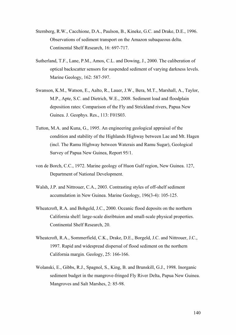
Sternberg, R.W., Cacchione, D.A., Paulson, B., Kineke, G.C. and Drake, D.E., 199
Observations of sediment transport on the Amazon subaqueous delta.
Continental Shelf Research, 16: 697-717.
6.
n of
ent of varying darkness levels.
Marine Geology, 162: 587-597.
Swanso er, J.W., Bera, M.T., Marshall, A., Taylor,
M.P., Apte, S.C. and Dietrich, W.E., 2008. Sediment load and floodplain
Tutton, M.A. and Kuna, G., 1995. An engineering geological appraisal of the
von de Borch, C.C., 1972. Marine geology
Wheatcrof
l of flood sediment on the northern
Wolanski, E., Gibbs, R.J., Spagnol, S., King,
uinea.
Sutherland, T.F., Lane, P.M., Amos, C.L. and Dowing, J., 2000. The caliberatio
optical backscatter sensors for suspended sedim
n, K.M., Watson, E., Aalto, R., Lau
deposition rates: Comparison of the Fly and Strickland rivers, Papua New
Guinea. J. Geophys. Res., 113: F01S03.
condition and stability of the Highlands Highway between Lae and Mt. Hagen
(incl. The Ramu Highway between Waterais and Ramu Sugar), Geological
Survey of Papua New Guinea, Report 95/1.
of Huon Gulf region, New Guinea. 127,
Department of National Development.
Walsh, J.P. and Nittrouer, C.A., 2003. Contrasting styles of off-shelf sediment
accumulation in New Guinea. Marine Geology, 196(3-4): 105-125.
Wheatcroft, R.A. and Bohgeld, J.C., 2000. Oceanic flood deposits on the northern
California shelf: large-scale disribtuion and small-scale physical properties.
Continental Shelf Research, 20.
t, R.A., Sommerfield, C.K., Drake, D.E., Borgeld, J.C. and Nittrouer, J.C.,
1997. Rapid and widespread dispersa
California margin. Geology, 25: 166-166.
B. and Brunskill, G.J., 1998. Inorganic
sediment budget in the mangrove-fringed Fly River Delta, Papua New G
Mangroves and Salt Marshes, 2: 85-98.
140
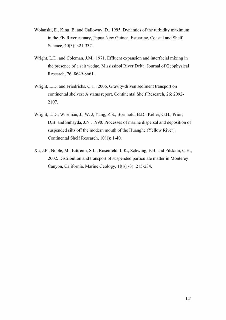
Wolanski, E., King, B. and Galloway, D., 1995. Dynamics of the turbidity maximum
in the Fly River estuary, Papua New Guinea. Estuarine, Coastal and Sh
Science, 40(3): 321-337.
elf
Wright, L.D., Wiseman, J., W. J, Yang, Z.S., Bornhold, B.D., Keller, G.H., Prior,
ition of
Xu, J.P., Noble, M., Eittreim, S.L., Rosenfeld, L.K., Schwing, F.B. and Pilskaln, C.H.,
1(1-3): 215-234.
Wright, L.D. and Coleman, J.M., 1971. Effluent expansion and interfacial mixing in
the presence of a salt wedge, Mississippi River Delta. Journal of Geophysical
Research, 76: 8649-8661.
Wright, L.D. and Friedrichs, C.T., 2006. Gravity-driven sediment transport on
continental shelves: A status report. Continental Shelf Research, 26: 2092-
2107.
D.B. and Suhayda, J.N., 1990. Processes of marine dispersal and depos
suspended silts off the modern mouth of the Huanghe (Yellow River).
Continental Shelf Research, 10(1): 1-40.
2002. Distribution and transport of suspended particulate matter in Monterey
Canyon, California. Marine Geology, 18
141
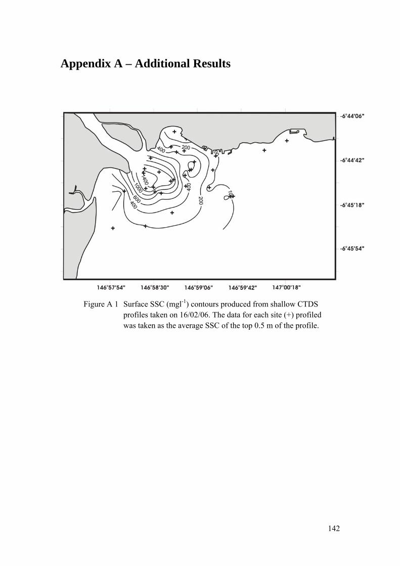
App
endix A – Additional Results
Figure A 1 Surface SSC (mgl-1) contours produced from shallow CTDS profiles taken on 16/02/06. The data for each site (+) profiled was taken as the average SSC of the top 0.5 m of the profile.
142
Figure A 2 Concurrent surface salinity (ppt) contours produced from shallow CTDS profiles taken on 16/02/06. The data for each site (+) profiled was taken as the average salinity of the top 0.5 m of the profile.
Figure A 3 SSC surface contours for profiles taken on 14/03/07 during intermediate discharge.
143
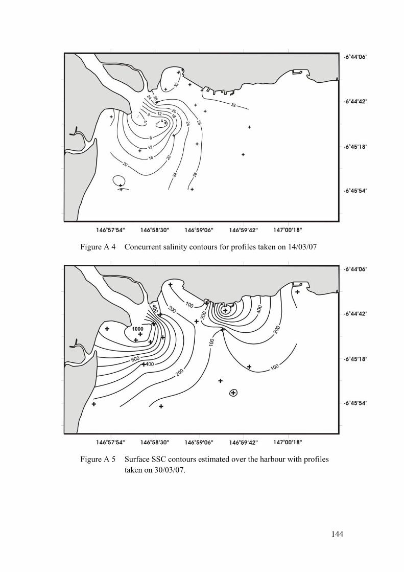
Figure A 4 Concurrent salinity contours for profiles taken on 14/03/07
Figure A 5 Surface SSC contours estimated over the harbour with profiles taken on 30/03/07.
144
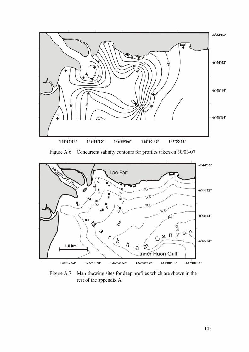
Figure A 6 Concurrent salinity contours for profiles taken on 30/03/07
Figure A 7 Map showing sites for deep profiles which are shown in the rest of the appendix A.
145
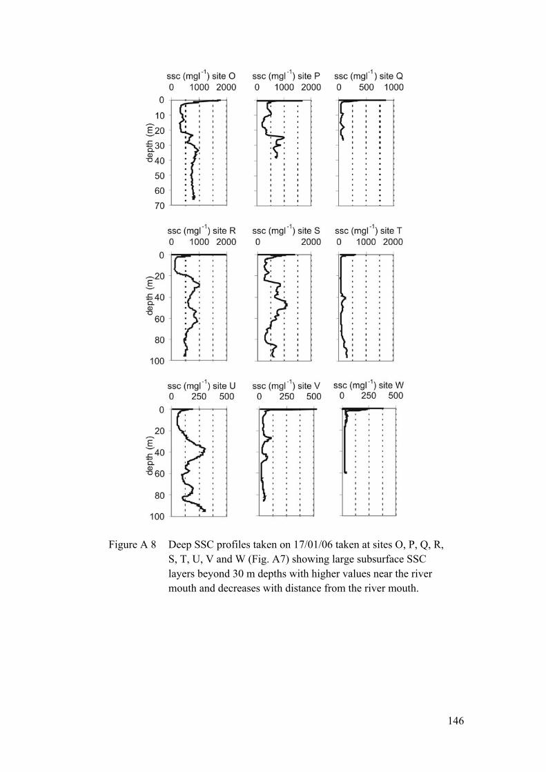
Figure A 8 Deep SSC profiles taken on 17/01/06 taken at sites O, P, Q, R, S, T, U, V and W (Fig. A7) showing large subsurface SSC layers beyond 30 m depths with higher values near the river mouth and decreases with distance from the river mouth.
146
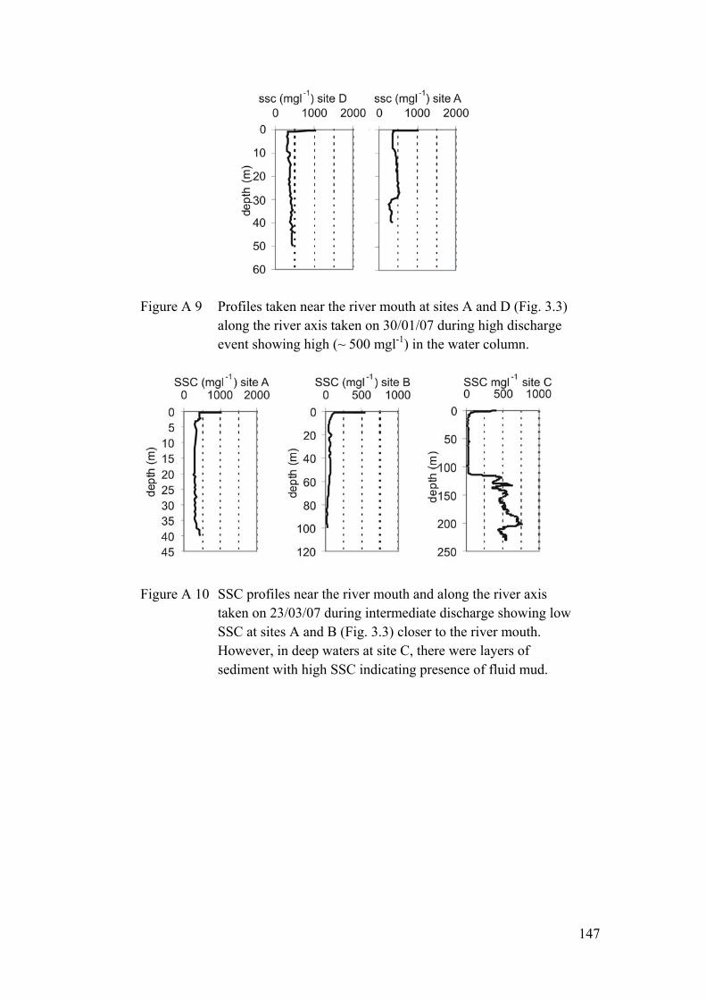
Figure A 9 Profiles taken near the river mouth at sites A and D (Fig. 3.3) along the river axis taken on 30/01/07 during high discharge event showing high (~ 500 mgl-1) in the water column.
Figure A 10 SSC profiles near the river mouth and along the river axis taken on 23/03/07 during intermediate discharge showing low SSC at sites A and B (Fig. 3.3) closer to the river mouth. However, in deep waters at site C, there were layers of sediment with high SSC indicating presence of fluid mud.
147
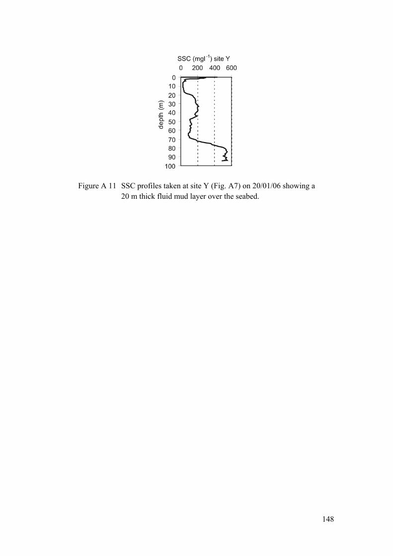
SSC profiles taken at site Y (Fig. A7) on 20/01/06 showing a 20 m thick fluid mud layer over the seabed.
Figure A 11
148

Appendix B – Specifications for Differential Pressure Sensor
DC001NDC4 Ultra-Low Pressure Sensors
DC Series, Bidirectional Gage, Differential; Signal Conditioning: Amplified; Pressure Range: ± 1.0 in H2O; Port Style: Barbed
Description
The ivity silicon sensing cap o produce one of the most precise, reliable pressure sensors in the market. The SURSENSE technology provides Dynamic Self Compensation which substantially reduces offset errors due to changes in temperature, stability to warmup, long term instability and position sensitivity. When operated with a fixed 5.0 Vdc supply the DC sensors provides a ratiometric 0.25 Vdc to 4.25 Vdc output (4.0 Vdc span). Regulated voltage units are also available for applications involving variable supply voltages (see electrical specifications).
Features Potential Applications
Features
Ultra Low Pressure Sensing, down to 1" H20
ASIC Enhanced Available in Gage and
Differential Pressure Ranges
Available in Ratiometric and Regulated
Temperature Compensated over 0 °C to 50 °C [32 °F to 122 °F]
Combined Linearity and Hysteresis error <�0.25% Span
Potential Applications
Medical Instrumentation HVAC Environmental Controls Portable Monitors
Product Specifications
Measurement Type Differential, Bidirectional Gage
Signal Conditioning Amplified
DC pressure sensor combines our SURSENSETM precision high sensitabilities with the latest in ASIC technology t
149
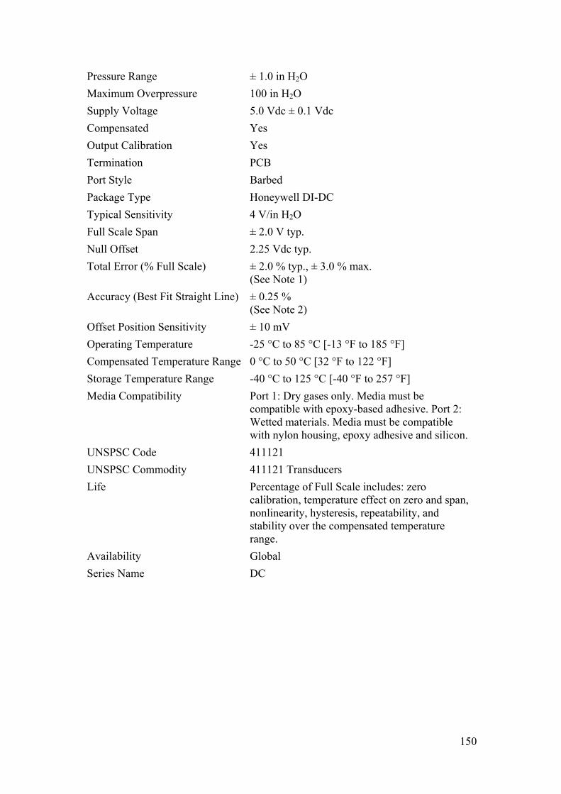
150
Supply Voltage 5.0 Vdc ± 0.1 Vdc
Compensated Yes
Termination PCB
Port Style
Package Type
sitivity
± 2.0 V typ.
2.25 Vdc typ.
ange -40 °C to 125 °C [-40 °F to 257 °F]
Media Comp Port 1: Dry g ased adhesive. Port 2:
ompatible e and silicon.
calibration, temperature effect on zero and span, nonlinearity, hysteresis, repeatability, and stability over the compensated temperature range.
Global
DC
Pressure Range ± 1.0 in H2O
Maximum Overpressure 100 in H2O
Output Calibration Yes
Barbed
Honeywell DI-DC
4 V/in H2O Typical Sen
Full Scale Span
Null Offset
Total Error (% Full Scale) ± 2.0 % typ., ± 3.0 % max. (See Note 1)
Accuracy (Best Fit Straight Line) ± 0.25 % (See Note 2)
Offset Position Sensitivity ± 10 mV
Operating Temperature -25 °C to 85 °C [-13 °F to 185 °F]
Compensated Temperature Range 0 °C to 50 °C [32 °F to 122 °F]
Storage Temperature R
atibility ases only. Media must becompatible with epoxy-bWe dtte materials. Media must be cwith n ing, epoxy adhesivylon hous
UNSPSC Code 411121
UNSPSC Commodity
Life
411121 Transducers
Percentage of Full Scale includes: zero
Availability
Series Name