Embed Size (px)
Citation preview
applied sciences
Article
Remote Servo Tuning System for Multi-Axis CNCMachine Tools Using a Virtual MachineTool Approach
Chien-Yu Lin and Ching-Hung Lee *
Department of Mechanical Engineering, National Chung Hsing University, Taichung 40227, Taiwan;[email protected]* Correspondence: [email protected]; Tel.: +886-4-2284-0433 (ext. 417); Fax: +886-2287-7170
Received: 14 June 2017; Accepted: 20 July 2017; Published: 30 July 2017
Abstract: Servo systems affect the performances of machining in accuracy and surface quality forhigh speed and precision machine tools. This study introduces an efficient servo tuning techniquefor Computer Numerical Control (CNC) feed drive systems using particle swarm optimization(PSO) algorithm by virtual machine tool approach. The proposed approach contained a systemidentification phase and a servo tuning phase based on the same bandwidth for all axes feed drivesystems. The PSO algorithm was adopted to obtain the system parameters and maximize thecorresponding bandwidth. An efficient two-step servo tuning method based on gain and phasemargins was proposed for high speed and precision requirements. All feed drive systems controllergains were optimized simultaneously for synchronization. A remote system called Machine Dr. wasestablished for servo tuning and monitoring. Simulation and experimental results were introducedto illustrate the effectiveness of the proposed approach.
Keywords: feed drive system; five axes; machine tools; servo tuning; particle swarm optimization
1. Introduction
Computer numerical control (CNC) machine tools have been widely used in high speed andprecision machining, such as curved surface, gears, aerospace materials, integrated circuit (IC) parts,and precision components, etc. This is why machine tool has been focused on how to accomplishhigh-speed and high-precision machining. Accurate control is required for machine tools to followthe desired contours. With increasing requirements for precision operations, many control strategieshave been proposed [1–11]. For industrial applications, the proportional-integral-derivative (PID)controllers of each axis are used for feed drive systems, therefore the tuning method for multi-axissynchronization for precision results are required. However, system dynamic parameters may beuncertain or vary with time. Thus, the system identification of feed drive systems should be donebefore tuning parameters. Some literature introduce virtual machine tools, including virtual CNC,servo models, and mechanical dynamics of feed drive systems, for treating the problem [11–19].
Feed drive systems may have unstable results or poor performance when servo parameters arenot designed properly [20,21]. Conventionally, the control gains of position and velocity controller areset as high as possible, under the condition that the stability and robustness of the closed loop systemis secured with some stability margins [21,22]. In general, each commercial CNC machine tool guidesthe user for tuning parameters step-by-step according to expert experience. In this study, we proposean intelligent and efficient method for the servo tuning problem to improve synchronization.
In order to employ the intelligent efficient method, this study developed a virtual CNC feeddrive system via system identification technology using Heidenhain TNCopt software. This canobtain the characteristics of the system and the mathematical models which we can use in numerical
Appl. Sci. 2017, 7, 776; doi:10.3390/app7080776 www.mdpi.com/journal/applsci
Appl. Sci. 2017, 7, 776 2 of 21
simulations; therefore, we were able to implement this intelligent and efficient method by anoptimization algorithm, e.g., a genetic algorithm, particle swarm optimization (PSO), evolutionaryalgorithm, electromagnetism-like algorithm, etc. [23–30]. In this study, the PSO was adopted forsolving optimization problems. As a result, combined with feed system signals processing andspectrum analysis, the servo system with mechanical dynamics was established. The intelligentalgorithm was used to automatically generate a set of suitable servo parameters for the currentmachine tool. After optimization, performance and processing quality would be better than the original.The proposed approach contained a system identification phase and a servo tuning phase based onthe same bandwidth for all axes feed drive systems. The particle swarm optimization algorithm wasadopted to obtain the system parameters and maximize the corresponding bandwidth. An efficienttwo-step servo tuning method based on gain and phase margins was proposed for high speed andprecision requirements. All feed drive systems controller gains were optimized simultaneously forsynchronization. Finally, the cloud computing system, called Machine Dr., was established for systemidentification, servo tuning, and monitoring.
This organization of this paper is introduced as follows. Section 2 introduces the preliminaries,including the modeling of feed drive systems, specification of machine tools, and the particle swarmoptimization algorithm. The proposed system identification based on PSO is introduced in Section 3.Section 4 introduces the intelligent servo tuning technique by two-step PSO. The correspondingsimulation, experimental results, and the Machine Dr. system are shown in Sections 3 and 4. Finally,the conclusion is given.
2. Preliminaries
This section introduces the preliminaries including feed drive system modeling, specifications offive-axis machine tools, and the particle swarm optimization algorithm.
2.1. Feed Drive Systems
Machine tool feed drive servo control systems are designed to accomplish a task, that is, to controlthe positions and velocities of machine tool axes in follow the commons generated by CNC controller.In general, the feed drive system contains two major parts. The first one is the electronic controlsystem or servo control system. The second one is the mechanical system such as the lead screw,bearing, motor, and worktable, etc. The servo system consists of plant, actuator, controller, and sensor.The control system with feedback is a closed-loop system, and without feedback is an open-loopsystem. The most common structure of servo control is closed loop, which belonging to passive control,and it has multiple loop characteristics and each loop has close relationships.
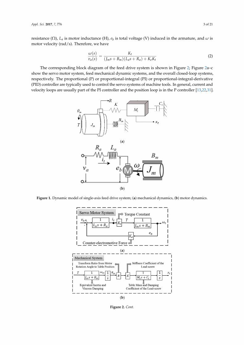
Many feed drive models have been proposed for system identification and controllerdesign [2,3,6,16,31,32]. Literature [31] proposes a virtual simulation model, the model contains theinfluence of the cutting force, friction and backlash nonlinear phenomenon. However, it assumes thatthe lead-screw is a rigid body, and the table mass and damping ratio were not considered. These reducethe accuracy and response of feed drive system. Figure 1 shows the dynamic model of the single-axisfeed drive system with mechanical vibration, where Jm: rotary inertia (kg·m2), Bm: damping coefficientof the rotary motion (Ns/m), Mt: table mass (kg), Ct: damping coefficient of the lead-screw (Ns/m), T:motor torque(Nm), K: stiffness coefficient of the lead-screw (N/m), θm: motor rotation angle (rad), xt:table position (m), R: transform ratio from motor rotation angle to table position (mm/rad) (R = p/2π),p is the lead-screw pitch (mm). The dynamic equation of this model can be expressed as:[
Jm 00 Mt
][ ..θm..xt
]+
[Bm 00 Mt
][ .θm.xt
]+
[R2K −RK−RK K
][θm
xt
]=
[T0
](1)
The schematic diagram for a motor is shown on Figure 1b, where va is separate input voltage (V),it is the circuit current (A) generated by the motor equivalent circuit impedance, Ra is motor equivalent
Appl. Sci. 2017, 7, 776 3 of 21
resistance (Ω), La is motor inductance (H), eb is total voltage (V) induced in the armature, and ω ismotor velocity (rad/s). Therefore, we have
ω(s)va(s)
=Kt
(Jms + Bm)(Las + Ra) + KeKt(2)
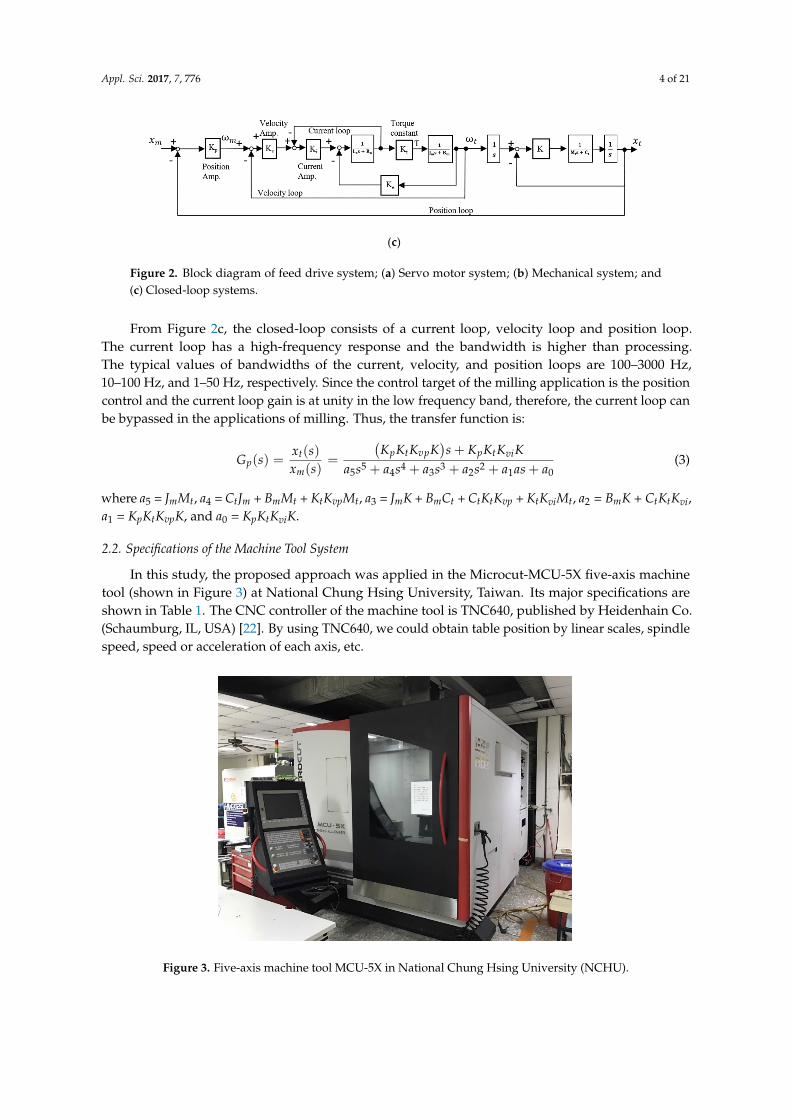
The corresponding block diagram of the feed drive system is shown in Figure 2; Figure 2a–cshow the servo motor system, feed mechanical dynamic systems, and the overall closed-loop systems,respectively. The proportional (P) or proportional-integral (PI) or proportional-integral-derivative(PID) controller are typically used to control the servo systems of machine tools. In general, current andvelocity loops are usually part of the PI controller and the position loop is in the P controller [13,22,31].
Appl. Sci. 2017, 7, 776 3 of 21
( )
( ) ( )( )t
a m m a a e t
Ks
v s J s B L s R K K
(2)
The corresponding block diagram of the feed drive system is shown in Figure 2; Figure 2a–c
show the servo motor system, feed mechanical dynamic systems, and the overall closed‐loop systems,
respectively. The proportional (P) or proportional‐integral (PI) or proportional‐integral‐derivative
(PID) controller are typically used to control the servo systems of machine tools. In general, current
and velocity loops are usually part of the PI controller and the position loop is in the P controller
[13,22,31].
(a)
(b)
Figure 1. Dynamic model of single‐axis feed drive system; (a) mechanical dynamics, (b) motor
dynamics.
(a)
(b)
Figure 1. Dynamic model of single-axis feed drive system; (a) mechanical dynamics, (b) motor dynamics.
Appl. Sci. 2017, 7, 776 3 of 21
( )
( ) ( )( )t
a m m a a e t
Ks
v s J s B L s R K K
(2)
The corresponding block diagram of the feed drive system is shown in Figure 2; Figure 2a–c
show the servo motor system, feed mechanical dynamic systems, and the overall closed‐loop systems,
respectively. The proportional (P) or proportional‐integral (PI) or proportional‐integral‐derivative
(PID) controller are typically used to control the servo systems of machine tools. In general, current
and velocity loops are usually part of the PI controller and the position loop is in the P controller
[13,22,31].
(a)
(b)
Figure 1. Dynamic model of single‐axis feed drive system; (a) mechanical dynamics, (b) motor
dynamics.
(a)
(b)
Figure 2. Cont.
Appl. Sci. 2017, 7, 776 4 of 21Appl. Sci. 2017, 7, 776 4 of 21
(c)
Figure 2. Block diagram of feed drive system; (a) Servo motor system; (b) Mechanical system; and (c)
Closed‐loop systems.
From Figure 2c, the closed‐loop consists of a current loop, velocity loop and position loop. The
current loop has a high‐frequency response and the bandwidth is higher than processing. The typical
values of bandwidths of the current, velocity, and position loops are 100–3000 Hz, 10–100 Hz, and 1–
50 Hz, respectively. Since the control target of the milling application is the position control and the
current loop gain is at unity in the low frequency band, therefore, the current loop can be bypassed
in the applications of milling. Thus, the transfer function is:
5 4 3 2
5 4 3 2 1 0
( )( )
( )
p t vp p t vitp
m
K K K K s K K K Kx sG s
x s a s a s a s a s a as a
(3)
where a5 = JmMt, a4 = CtJm + BmMt + KtKvpMt, a3 = JmK + BmCt + CtKtKvp + KtKviMt, a2 = BmK + CtKtKvi, a1 =
KpKtKvpK, and a0 = KpKtKviK.
2.2. Specifications of the Machine Tool System
In this study, the proposed approach was applied in the Microcut‐MCU‐5X five‐axis machine
tool (shown in Figure 3) at National Chung Hsing University, Taiwan. Its major specifications are
shown in Table 1. The CNC controller of the machine tool is TNC640, published by Heidenhain Co.
(Schaumburg, IL, USA) [22]. By using TNC640, we could obtain table position by linear scales, spindle
speed, speed or acceleration of each axis, etc.
Table 1. Major specifications of the machine tool (MCU‐5X).
Specifications Values
X/Y/Z Axis Travel (mm) 600/600/500
Tilting Axis A (degree) +120/−120
Rotary C (degree) 360
Rapid Traverse X/Y/Z (mm/min) 36,000/36,000/36,000
Max. Speed A/C (rpm) 16.6/90
Spindle Speed Range (rpm) 12,000 (std)/15,000 (opt)
Type of Position Control Full‐closed control
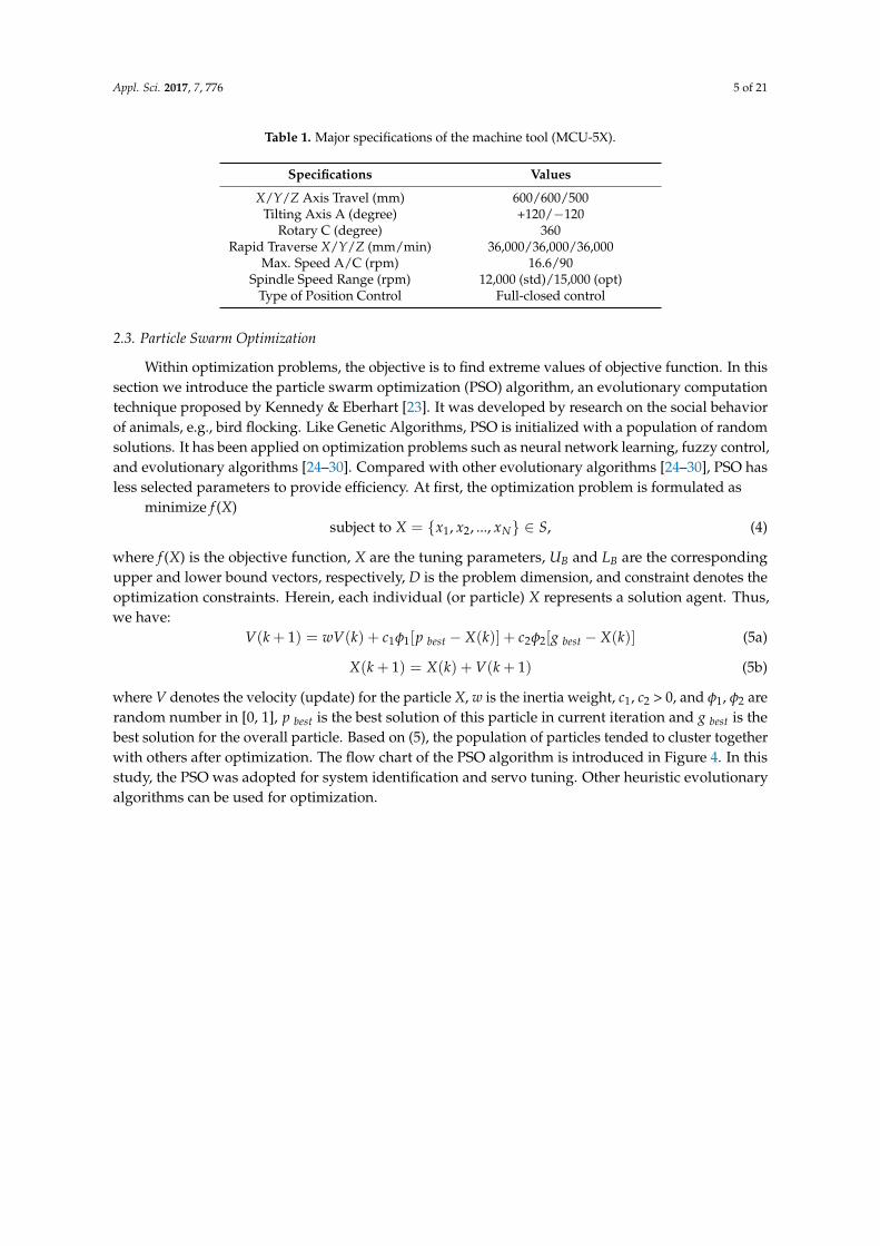
Figure 2. Block diagram of feed drive system; (a) Servo motor system; (b) Mechanical system; and(c) Closed-loop systems.
From Figure 2c, the closed-loop consists of a current loop, velocity loop and position loop.The current loop has a high-frequency response and the bandwidth is higher than processing.The typical values of bandwidths of the current, velocity, and position loops are 100–3000 Hz,10–100 Hz, and 1–50 Hz, respectively. Since the control target of the milling application is the positioncontrol and the current loop gain is at unity in the low frequency band, therefore, the current loop canbe bypassed in the applications of milling. Thus, the transfer function is:
Gp(s) =xt(s)xm(s)
=
(KpKtKvpK
)s + KpKtKviK
a5s5 + a4s4 + a3s3 + a2s2 + a1as + a0(3)
where a5 = JmMt, a4 = CtJm + BmMt + KtKvpMt, a3 = JmK + BmCt + CtKtKvp + KtKviMt, a2 = BmK + CtKtKvi,a1 = KpKtKvpK, and a0 = KpKtKviK.
2.2. Specifications of the Machine Tool System
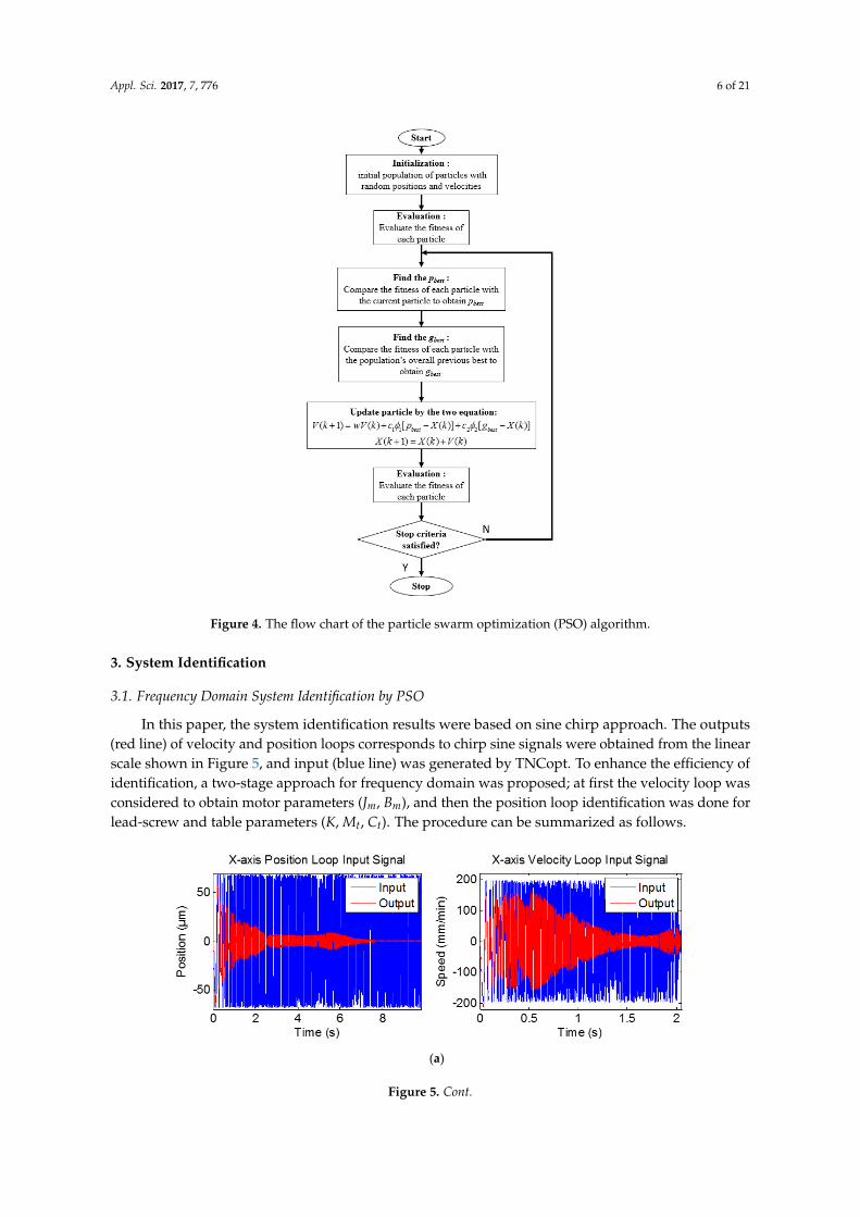
In this study, the proposed approach was applied in the Microcut-MCU-5X five-axis machinetool (shown in Figure 3) at National Chung Hsing University, Taiwan. Its major specifications areshown in Table 1. The CNC controller of the machine tool is TNC640, published by Heidenhain Co.(Schaumburg, IL, USA) [22]. By using TNC640, we could obtain table position by linear scales, spindlespeed, speed or acceleration of each axis, etc.Appl. Sci. 2017, 7, 776 5 of 21
Figure 3. Five‐axis machine tool MCU‐5X in National Chung Hsing University (NCHU).
2.3. Particle Swarm Optimization
Within optimization problems, the objective is to find extreme values of objective function. In
this section we introduce the particle swarm optimization (PSO) algorithm, an evolutionary
computation technique proposed by Kennedy & Eberhart [23]. It was developed by research on the
social behavior of animals, e.g., bird flocking. Like Genetic Algorithms, PSO is initialized with a
population of random solutions. It has been applied on optimization problems such as neural
network learning, fuzzy control, and evolutionary algorithms [24–30]. Compared with other
evolutionary algorithms [24–30], PSO has less selected parameters to provide efficiency. At first, the
optimization problem is formulated as
minimize f(X)
1 2subject to , , ..., NX x x x S , (4)
where f(X) is the objective function, X are the tuning parameters, UB and LB are the corresponding
upper and lower bound vectors, respectively, D is the problem dimension, and constraint denotes
the optimization constraints. Herein, each individual (or particle) X represents a solution agent. Thus,
we have:
)]([)]([)()1( 2211 kXgckXpckwVkV bestbest (5a)
)1()()1( kVkXkX (5b)
where V denotes the velocity (update) for the particle X, w is the inertia weight, c1, c2 > 0, and 1 , 2 are random number in [0, 1], bestp is the best solution of this particle in current iteration and bestg is
the best solution for the overall particle. Based on (5), the population of particles tended to cluster
together with others after optimization. The flow chart of the PSO algorithm is introduced in Figure
4. In this study, the PSO was adopted for system identification and servo tuning. Other heuristic
evolutionary algorithms can be used for optimization.
Figure 3. Five-axis machine tool MCU-5X in National Chung Hsing University (NCHU).
Appl. Sci. 2017, 7, 776 5 of 21
Table 1. Major specifications of the machine tool (MCU-5X).
Specifications Values
X/Y/Z Axis Travel (mm) 600/600/500Tilting Axis A (degree) +120/−120
Rotary C (degree) 360Rapid Traverse X/Y/Z (mm/min) 36,000/36,000/36,000
Max. Speed A/C (rpm) 16.6/90Spindle Speed Range (rpm) 12,000 (std)/15,000 (opt)
Type of Position Control Full-closed control
2.3. Particle Swarm Optimization
Within optimization problems, the objective is to find extreme values of objective function. In thissection we introduce the particle swarm optimization (PSO) algorithm, an evolutionary computationtechnique proposed by Kennedy & Eberhart [23]. It was developed by research on the social behaviorof animals, e.g., bird flocking. Like Genetic Algorithms, PSO is initialized with a population of randomsolutions. It has been applied on optimization problems such as neural network learning, fuzzy control,and evolutionary algorithms [24–30]. Compared with other evolutionary algorithms [24–30], PSO hasless selected parameters to provide efficiency. At first, the optimization problem is formulated as
minimize f (X)subject to X = x1, x2, ..., xN ∈ S, (4)
where f (X) is the objective function, X are the tuning parameters, UB and LB are the correspondingupper and lower bound vectors, respectively, D is the problem dimension, and constraint denotes theoptimization constraints. Herein, each individual (or particle) X represents a solution agent. Thus,we have:
V(k + 1) = wV(k) + c1φ1[p best − X(k)] + c2φ2[g best − X(k)] (5a)
X(k + 1) = X(k) + V(k + 1) (5b)
where V denotes the velocity (update) for the particle X, w is the inertia weight, c1, c2 > 0, and φ1, φ2 arerandom number in [0, 1], p best is the best solution of this particle in current iteration and g best is thebest solution for the overall particle. Based on (5), the population of particles tended to cluster togetherwith others after optimization. The flow chart of the PSO algorithm is introduced in Figure 4. In thisstudy, the PSO was adopted for system identification and servo tuning. Other heuristic evolutionaryalgorithms can be used for optimization.
Appl. Sci. 2017, 7, 776 6 of 21Appl. Sci. 2017, 7, 776 6 of 21
Figure 4. The flow chart of the particle swarm optimization (PSO) algorithm.
3. System Identification
3.1. Frequency Domain System Identification by PSO
In this paper, the system identification results were based on sine chirp approach. The outputs
(red line) of velocity and position loops corresponds to chirp sine signals were obtained from the
linear scale shown in Figure 5, and input (blue line) was generated by TNCopt. To enhance the
efficiency of identification, a two‐stage approach for frequency domain was proposed; at first the
velocity loop was considered to obtain motor parameters (Jm, Bm), and then the position loop
identification was done for lead‐screw and table parameters (K, Mt, Ct). The procedure can be
summarized as follows.
(a)
Figure 4. The flow chart of the particle swarm optimization (PSO) algorithm.
3. System Identification
3.1. Frequency Domain System Identification by PSO
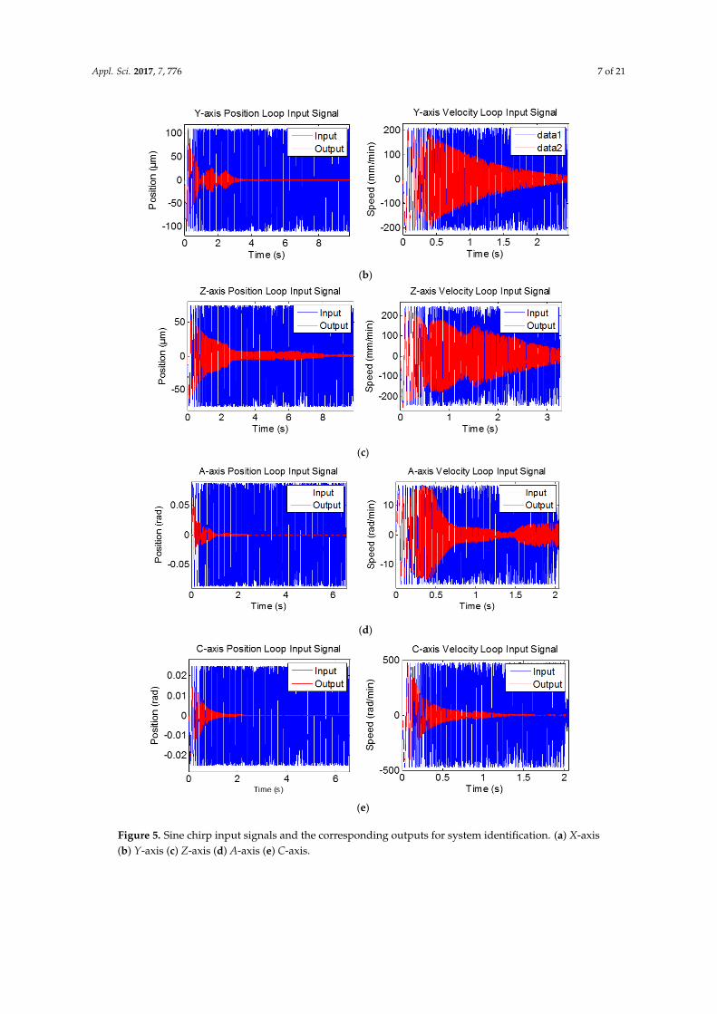
In this paper, the system identification results were based on sine chirp approach. The outputs(red line) of velocity and position loops corresponds to chirp sine signals were obtained from the linearscale shown in Figure 5, and input (blue line) was generated by TNCopt. To enhance the efficiency ofidentification, a two-stage approach for frequency domain was proposed; at first the velocity loop wasconsidered to obtain motor parameters (Jm, Bm), and then the position loop identification was done forlead-screw and table parameters (K, Mt, Ct). The procedure can be summarized as follows.
Appl. Sci. 2017, 7, 776 6 of 21
Figure 4. The flow chart of the particle swarm optimization (PSO) algorithm.
3. System Identification
3.1. Frequency Domain System Identification by PSO
In this paper, the system identification results were based on sine chirp approach. The outputs
(red line) of velocity and position loops corresponds to chirp sine signals were obtained from the
linear scale shown in Figure 5, and input (blue line) was generated by TNCopt. To enhance the
efficiency of identification, a two‐stage approach for frequency domain was proposed; at first the
velocity loop was considered to obtain motor parameters (Jm, Bm), and then the position loop
identification was done for lead‐screw and table parameters (K, Mt, Ct). The procedure can be
summarized as follows.
(a)
Figure 5. Cont.
Appl. Sci. 2017, 7, 776 7 of 21Appl. Sci. 2017, 7, 776 7 of 21
(b)
(c)
(d)
(e)
Figure 5. Sine chirp input signals and the corresponding outputs for system identification. (a) X‐axis
(b) Y‐axis (c) Z‐axis (d) A‐axis (e) C‐axis.
Procedure 1: System Identification
Figure 5. Sine chirp input signals and the corresponding outputs for system identification. (a) X-axis(b) Y-axis (c) Z-axis (d) A-axis (e) C-axis.
Appl. Sci. 2017, 7, 776 8 of 21
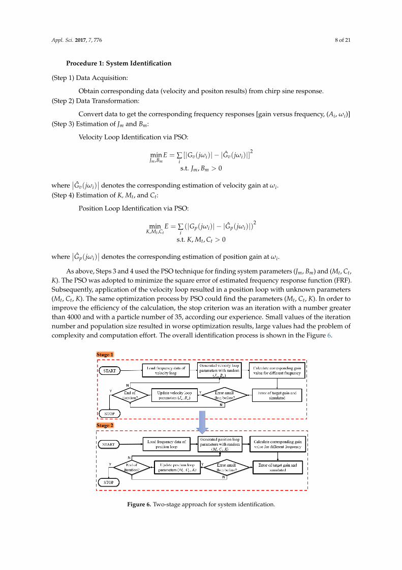
Procedure 1: System Identification
(Step 1) Data Acquisition:
Obtain corresponding data (velocity and positon results) from chirp sine response.(Step 2) Data Transformation:
Convert data to get the corresponding frequency responses [gain versus frequency, (Ai, ωi)](Step 3) Estimation of Jm and Bm:
Velocity Loop Identification via PSO:
minJm ,Bm
E = ∑i[|Gv(jωi)| − |Gv(jωi)|]
2
s.t. Jm, Bm > 0
where∣∣Gv(jωi)
∣∣ denotes the corresponding estimation of velocity gain at ωi.(Step 4) Estimation of K, Mt, and Ct:
Position Loop Identification via PSO:
minK,Mt ,Ct
E = ∑i(|Gp(jωi)| − |Gp(jωi)|)
2
s.t. K, Mt, Ct > 0
where∣∣Gp(jωi)
∣∣ denotes the corresponding estimation of position gain at ωi.
As above, Steps 3 and 4 used the PSO technique for finding system parameters (Jm, Bm) and (Mt, Ct,K). The PSO was adopted to minimize the square error of estimated frequency response function (FRF).Subsequently, application of the velocity loop resulted in a position loop with unknown parameters(Mt, Ct, K). The same optimization process by PSO could find the parameters (Mt, Ct, K). In order toimprove the efficiency of the calculation, the stop criterion was an iteration with a number greaterthan 4000 and with a particle number of 35, according our experience. Small values of the iterationnumber and population size resulted in worse optimization results, large values had the problem ofcomplexity and computation effort. The overall identification process is shown in the Figure 6.
Appl. Sci. 2017, 7, 776 8 of 21
(Step 1) Data Acquisition:
Obtain corresponding data (velocity and positon results) from chirp sine response.
(Step 2) Data Transformation:
Convert data to get the corresponding frequency responses [gain versus frequency, (Ai,
ωi)]
(Step 3) Estimation of Jm and Bm:
Velocity Loop Identification via PSO:
2
,
ˆmin [| ( )| | ( )|]
s.t. , 0m m
v i v iJ Bi
m m
E G j G j
J B
where ˆ ( )v iG j denotes the corresponding estimation of velocity gain at ωi.
(Step 4) Estimation of K, Mt, and Ct:
Position Loop Identification via PSO:
2
, ,
ˆmin (| ( )| | ( )|)
s.t. , , 0t t
p i p iK M Ci
t t
E G j G j
K M C
where ˆ ( )p iG j denotes the corresponding estimation of position gain at ωi.
As above, Steps 3 and 4 used the PSO technique for finding system parameters (Jm, Bm) and (Mt,
Ct, K). The PSO was adopted to minimize the square error of estimated frequency response function
(FRF). Subsequently, application of the velocity loop resulted in a position loop with unknown
parameters (Mt, Ct, K). The same optimization process by PSO could find the parameters (Mt, Ct, K).
In order to improve the efficiency of the calculation, the stop criterion was an iteration with a number
greater than 4000 and with a particle number of 35, according our experience. Small values of the
iteration number and population size resulted in worse optimization results, large values had the
problem of complexity and computation effort. The overall identification process is shown in the
Figure 6.
Figure 6. Two‐stage approach for system identification.
3.2. Identification Results
Herein, the identification results of MCU‐5X are introduced by our approach. We obtained
system parameters (Jm, Bm, Mt, Ct, K) of axes feed drive systems and the corresponding transfer
function in form of (3). For the velocity loop, the corresponding frequency responses of the actual
system and estimation system are shown in Figure 7 (solid‐line: experimental results; dotted‐line:
Figure 6. Two-stage approach for system identification.
Appl. Sci. 2017, 7, 776 9 of 21
3.2. Identification Results
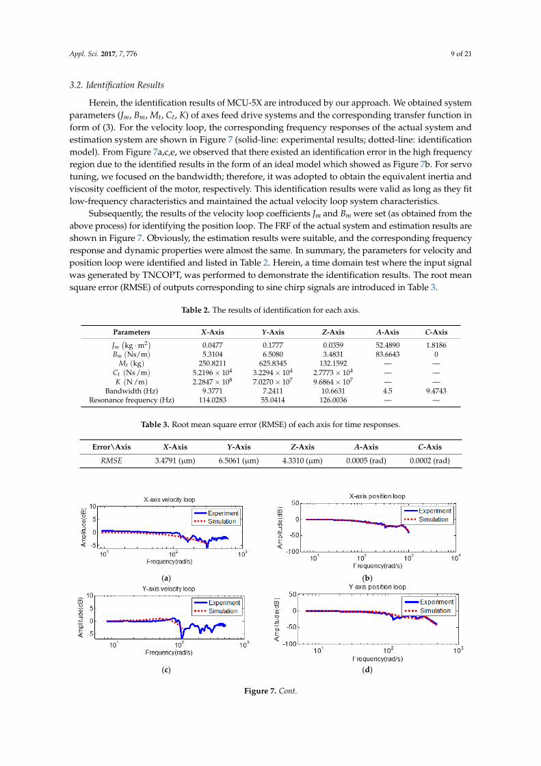
Herein, the identification results of MCU-5X are introduced by our approach. We obtained systemparameters (Jm, Bm, Mt, Ct, K) of axes feed drive systems and the corresponding transfer function inform of (3). For the velocity loop, the corresponding frequency responses of the actual system andestimation system are shown in Figure 7 (solid-line: experimental results; dotted-line: identificationmodel). From Figure 7a,c,e, we observed that there existed an identification error in the high frequencyregion due to the identified results in the form of an ideal model which showed as Figure 7b. For servotuning, we focused on the bandwidth; therefore, it was adopted to obtain the equivalent inertia andviscosity coefficient of the motor, respectively. This identification results were valid as long as they fitlow-frequency characteristics and maintained the actual velocity loop system characteristics.
Subsequently, the results of the velocity loop coefficients Jm and Bm were set (as obtained from theabove process) for identifying the position loop. The FRF of the actual system and estimation results areshown in Figure 7. Obviously, the estimation results were suitable, and the corresponding frequencyresponse and dynamic properties were almost the same. In summary, the parameters for velocity andposition loop were identified and listed in Table 2. Herein, a time domain test where the input signalwas generated by TNCOPT, was performed to demonstrate the identification results. The root meansquare error (RMSE) of outputs corresponding to sine chirp signals are introduced in Table 3.
Table 2. The results of identification for each axis.
Parameters X-Axis Y-Axis Z-Axis A-Axis C-Axis
Jm(kg ·m2) 0.0477 0.1777 0.0359 52.4890 1.8186
Bm (Ns/m) 5.3104 6.5080 3.4831 83.6643 0Mt (kg) 250.8211 625.8345 132.1592 — —
Ct (Ns /m) 5.2196× 10⁴ 3.2294× 10⁴ 2.7773× 10⁴ — —K (N /m) 2.2847× 10⁸ 7.0270× 10⁷ 9.6864× 10⁷ — —
Bandwidth (Hz) 9.3771 7.2411 10.6631 4.5 9.4743Resonance frequency (Hz) 114.0283 55.0414 126.0036 — —
Table 3. Root mean square error (RMSE) of each axis for time responses.
Error\Axis X-Axis Y-Axis Z-Axis A-Axis C-Axis
RMSE 3.4791 (µm) 6.5061 (µm) 4.3310 (µm) 0.0005 (rad) 0.0002 (rad)
Appl. Sci. 2017, 7, 776 9 of 21
identification model). From Figure 7a,c,e, we observed that there existed an identification error in the
high frequency region due to the identified results in the form of an ideal model which showed as
Figure 7b. For servo tuning, we focused on the bandwidth; therefore, it was adopted to obtain the
equivalent inertia and viscosity coefficient of the motor, respectively. This identification results were
valid as long as they fit low‐frequency characteristics and maintained the actual velocity loop system
characteristics.
Subsequently, the results of the velocity loop coefficients Jm and Bm were set (as obtained from
the above process) for identifying the position loop. The FRF of the actual system and estimation
results are shown in Figure 7. Obviously, the estimation results were suitable, and the corresponding
frequency response and dynamic properties were almost the same. In summary, the parameters for
velocity and position loop were identified and listed in Table 2. Herein, a time domain test where the
input signal was generated by TNCOPT, was performed to demonstrate the identification results.
The root mean square error (RMSE) of outputs corresponding to sine chirp signals are introduced in
Table 3.
Table 2. The results of identification for each axis.
Parameters X‐axis Y‐axis Z‐axis A‐axis C‐axis
Jm 2(kg m ) 0.0477 0.1777 0.0359 52.4890 1.8186
Bm )mNs( 5.3104 6.5080 3.4831 83.6643 0
Mt (kg) 250.8211 625.8345 132.1592 ‐‐‐ ‐‐‐
Ct (Ns m) 5.2196 10 3.2294 104 2.7773 104 ‐‐‐ ‐‐‐
K (N m) 2.2847 108 7.0270 10 9.6864 107 ‐‐‐ ‐‐‐
Bandwidth (Hz) 9.3771 7.2411 10.6631 4.5 9.4743Resonance frequency (Hz) 114.0283 55.0414 126.0036 ‐‐‐ ‐‐‐
Table 3. Root mean square error (RMSE) of each axis for time responses.
Error\Axis X‐axis Y‐axis Z‐axis A‐axis C‐axis
RMSE 3.4791 (µm) 6.5061 (µm) 4.3310 (µm) 0.0005 (rad) 0.0002 (rad)
(a) (b)
(c) (d)
Figure 7. Cont.
Appl. Sci. 2017, 7, 776 10 of 21Appl. Sci. 2017, 7, 776 10 of 21
(e) (f)
(g) (h)
(i) (j)
Figure 7. Frequency responses of velocity loop and position loop. (a) X‐axis: velocity loop. (b) X‐axis:
position loop. (c) Y‐axis: velocity loop. (d) Y‐axis: position loop. (e) Z‐axis: velocity loop. (f) Z‐axis:
position loop. (g) A‐axis: velocity loop. (h) A‐axis: position loop. (i) C‐axis: velocity loop. (j) C‐axis:
position loop.
To verify the model obtained from system identification, another illustration example was
introduced. We changed the servo parameters Kpp, Kvi, and Kvp to have the FRF of the actual
experimental results (machine tool results) and the identified results. Figure 8 shows the
identification results of the X‐axis, Y‐axis, Z‐axis, A‐axis, and C‐axis, respectively. The blue line in
Figure 8a–e are the FRF of default servo parameters, which we employed in system identification.
The black line in Figure 8a–e are the FRF of changed servo parameters which were obtained by MCU‐
5X. Both dotted red lines represent the simulation FRF of the default and change servo parameters.
It was confirmed that the system identification process was reliable.
(a)
101
102
103
-40
-30
-20
-10
0
X-axis position loop
Frequency(rad/s)
Am
plit
ud
e(d
B)
Experiment (Kp=92 Kvp=8 Kvi=800)Simulation (Kp=92 Kvp=8 Kvi=800)Experiment (Kp=48 Kvp=10 Kvi=1000)Simulation (Kp=48 Kvp=10 Kvi=1000)
Figure 7. Frequency responses of velocity loop and position loop. (a) X-axis: velocity loop. (b) X-axis:position loop. (c) Y-axis: velocity loop. (d) Y-axis: position loop. (e) Z-axis: velocity loop. (f) Z-axis:position loop. (g) A-axis: velocity loop. (h) A-axis: position loop. (i) C-axis: velocity loop. (j) C-axis:position loop.
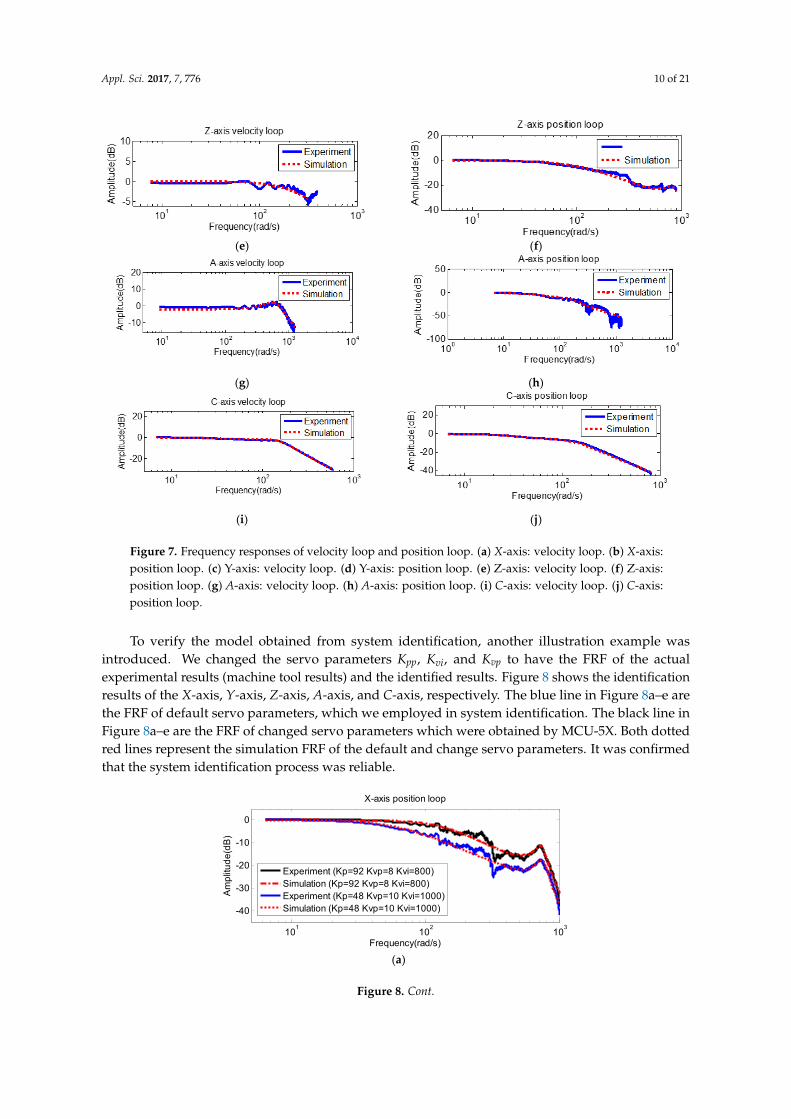
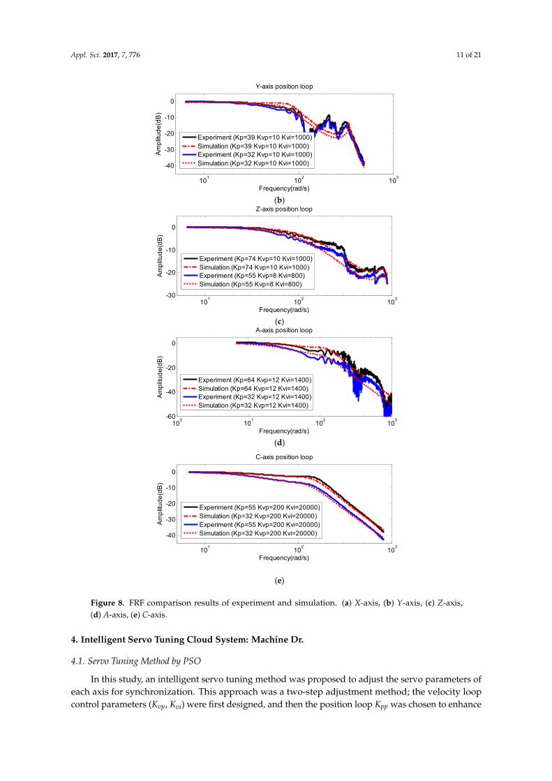
To verify the model obtained from system identification, another illustration example wasintroduced. We changed the servo parameters Kpp, Kvi, and Kvp to have the FRF of the actualexperimental results (machine tool results) and the identified results. Figure 8 shows the identificationresults of the X-axis, Y-axis, Z-axis, A-axis, and C-axis, respectively. The blue line in Figure 8a–e arethe FRF of default servo parameters, which we employed in system identification. The black line inFigure 8a–e are the FRF of changed servo parameters which were obtained by MCU-5X. Both dottedred lines represent the simulation FRF of the default and change servo parameters. It was confirmedthat the system identification process was reliable.
Appl. Sci. 2017, 7, 776 10 of 21
(e) (f)
(g) (h)
(i) (j)
Figure 7. Frequency responses of velocity loop and position loop. (a) X‐axis: velocity loop. (b) X‐axis:
position loop. (c) Y‐axis: velocity loop. (d) Y‐axis: position loop. (e) Z‐axis: velocity loop. (f) Z‐axis:
position loop. (g) A‐axis: velocity loop. (h) A‐axis: position loop. (i) C‐axis: velocity loop. (j) C‐axis:
position loop.
To verify the model obtained from system identification, another illustration example was
introduced. We changed the servo parameters Kpp, Kvi, and Kvp to have the FRF of the actual
experimental results (machine tool results) and the identified results. Figure 8 shows the
identification results of the X‐axis, Y‐axis, Z‐axis, A‐axis, and C‐axis, respectively. The blue line in
Figure 8a–e are the FRF of default servo parameters, which we employed in system identification.
The black line in Figure 8a–e are the FRF of changed servo parameters which were obtained by MCU‐
5X. Both dotted red lines represent the simulation FRF of the default and change servo parameters.
It was confirmed that the system identification process was reliable.
(a)
101
102
103
-40
-30
-20
-10
0
X-axis position loop
Frequency(rad/s)
Am
plit
ud
e(d
B)
Experiment (Kp=92 Kvp=8 Kvi=800)Simulation (Kp=92 Kvp=8 Kvi=800)Experiment (Kp=48 Kvp=10 Kvi=1000)Simulation (Kp=48 Kvp=10 Kvi=1000)
Figure 8. Cont.
Appl. Sci. 2017, 7, 776 11 of 21
Appl. Sci. 2017, 7, 776 11 of 21
(b)
(c)
(d)
(e)
Figure 8. FRF comparison results of experiment and simulation. (a) X‐axis, (b) Y‐axis, (c) Z‐axis, (d)
A‐axis, (e) C‐axis.
4. Intelligent Servo Tuning Cloud System: Machine Dr.
4.1. Servo Tuning Method by PSO
In this study, an intelligent servo tuning method was proposed to adjust the servo parameters
of each axis for synchronization. This approach was a two‐step adjustment method; the velocity loop
control parameters (Kvp, Kvi) were first designed, and then the position loop Kpp was chosen to enhance
the bandwidth at several constraints. Figure 8 shows the flow chart of the proposed method, it
contains data acquisition, system identification, virtual servo system setup, parameters optimization
of velocity loop, and parameters optimization of the position loop. After data analysis and system
101
102
103
-40
-30
-20
-10
0
Y-axis position loop
Frequency(rad/s)
Am
plit
ud
e(d
B)
Experiment (Kp=39 Kvp=10 Kvi=1000)Simulation (Kp=39 Kvp=10 Kvi=1000)Experiment (Kp=32 Kvp=10 Kvi=1000)Simulation (Kp=32 Kvp=10 Kvi=1000)
101
102
103
-30
-20
-10
0
Z-axis position loop
Frequency(rad/s)
Am
plit
ud
e(d
B)
Experiment (Kp=74 Kvp=10 Kvi=1000)Simulation (Kp=74 Kvp=10 Kvi=1000)Experiment (Kp=55 Kvp=8 Kvi=800)Simulation (Kp=55 Kvp=8 Kvi=800)
100
101
102
103
-60
-40
-20
0
A-axis position loop
Frequency(rad/s)
Am
plit
ud
e(d
B)
Experiment (Kp=64 Kvp=12 Kvi=1400)Simulation (Kp=64 Kvp=12 Kvi=1400)Experiment (Kp=32 Kvp=12 Kvi=1400)Simulation (Kp=32 Kvp=12 Kvi=1400)
101
102
103
-40
-30
-20
-10
0
Frequency(rad/s)
Am
plit
ud
e(d
B)
C-axis position loop
Experiment (Kp=55 Kvp=200 Kvi=20000)Simulation (Kp=32 Kvp=200 Kvi=20000)Experiment (Kp=55 Kvp=200 Kvi=20000)Simulation (Kp=32 Kvp=200 Kvi=20000)
Figure 8. FRF comparison results of experiment and simulation. (a) X-axis, (b) Y-axis, (c) Z-axis,(d) A-axis, (e) C-axis.
4. Intelligent Servo Tuning Cloud System: Machine Dr.
4.1. Servo Tuning Method by PSO
In this study, an intelligent servo tuning method was proposed to adjust the servo parameters ofeach axis for synchronization. This approach was a two-step adjustment method; the velocity loopcontrol parameters (Kvp, Kvi) were first designed, and then the position loop Kpp was chosen to enhance
Appl. Sci. 2017, 7, 776 12 of 21
the bandwidth at several constraints. Figure 8 shows the flow chart of the proposed method, it containsdata acquisition, system identification, virtual servo system setup, parameters optimization of velocityloop, and parameters optimization of the position loop. After data analysis and system identification,we established the virtual system of the feed drive. By using the virtual model, the PSO was adopted tooptimize velocity controllers of five axes in the same bandwidth for synchronization. In this procedure,velocity loop servo parameters (Kvp, Kvi) of each axis were obtained by PSO with constraints.
Maximize BWvel.
Subject to Max|Gv(iw)| ≤ 1Gain margin (GM) > 10 dBPhase margin (PM) > 45.
where BWvel. denotes the bandwidth of velocity loop. According our experience, excessive gainof FRF may result unstable and vibrations. We used this Constraint 1 to ensure that the system wasstable and vibration was low. Constraints 2 and 3 related to gain margin (GM) and phase margin (PM).GM and PM are widely used to confirm system stability and robustness. Herein, for the initialization ofPSO, the default values were assigned to be for initial particles; thus, the tuning method would ensurethat bandwidth would not decrease. By this method, we obtained velocity controller parameterswith better bandwidth. After updating the velocity servo parameters, we then optimized the positioncontroller (Kpp). Similar to velocity loop, we have:
Maximize BWpos.
Subject to Max∣∣Gp(iw)
∣∣ ≤ 1Gain margin (GM) > 15 dBPhase margin (PM) > 45
BWpos. <BWvel.
3
where BWpos. denotes the bandwidth of the position loop.
Note that Constraint 4, BWpos. <BWvel.
3 , ensured system stability and only a small overshoot ofthe time response [33].
4.2. Comparison Results-One and Two Steps Optimization
Herein, we had a comparison of results of illustration for our approach. The tuning parameters(Kvp, Kvi, Kpp) were optimized simultaneously and by two-step optimization. Our approach was atwo-step method, where the velocity loop control parameter (Kvp, Kvi) were first designed, and thenthe position loop Kpp was chosen to enhance the bandwidth, shown in Figure 9. Table 4 shows thecomparison results of tuning results between one-step and two-steps. We found that the computationeffort was reduced by our approach. An almost 50% improvement in computation time was saved.In summary, the two-step was better than the one-step in various aspects.
Appl. Sci. 2017, 7, 776 13 of 21Appl. Sci. 2017, 7, 776 13 of 21
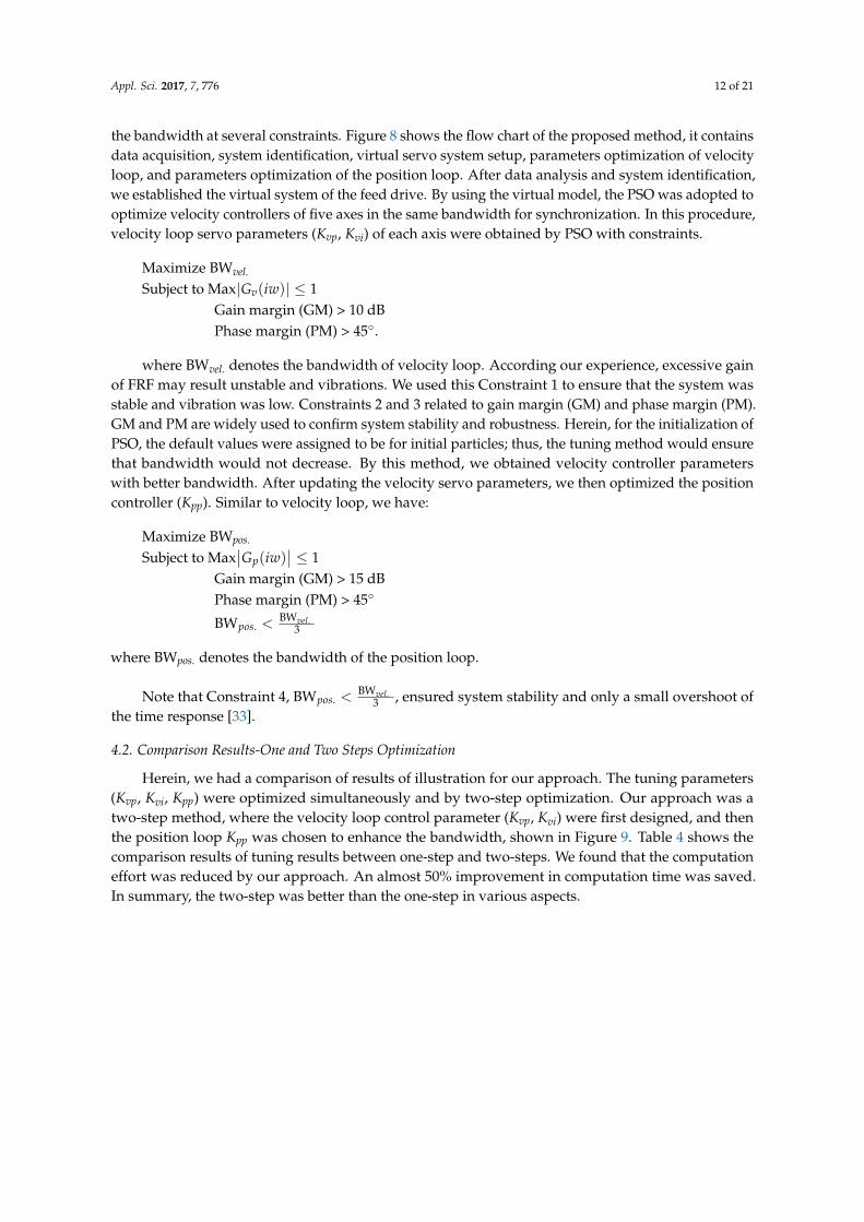
Figure 9. Intelligent tuning servo system flowchart.
Table 4. Comparison results of tuning results between one‐step and two‐steps.
Two‐Step 1 2 3 4 5 6
Time (s) 199.9 210.8 323.5 344.4 513.3 501.9
Bandwidth (rad/s) 81.23 82.95 82.95 84.55 84.55 84.55
Particle (PSO) 25 30 30 35 35 40
Iteration (PSO) 200 200 500 500 600 600
One‐Step 1 2 3 4 5 6
Time (sec) 371.7 440.5 687.2 712.9 833.4 904.2
Bandwidth (rad/s) 42.58 27.33 41.14 43.64 42.74 79.18
Particle (PSO) 25 30 30 35 35 40
Iteration (PSO) 200 200 500 500 600 600
4.3. Machine Dr. System Development
We developed a platform to implement remote connection with machine tools, where the user
could connect the machine tools and obtain the status of machines via the internet, called Machine
Dr.; the functions illustration is shown in Figure 10. It is based on system identification, intelligent
tuning servo systems, database processing, and cloud computing. Figure 10b illustrates the
communication between machine tools and users. After receiving system identification data,
Machine Dr. calculates the associated information of the machine and establishes corresponding data
in the cloud, and then Machine Dr. also provides identification results and suggested P‐PI controller
Figure 9. Intelligent tuning servo system flowchart.
Table 4. Comparison results of tuning results between one-step and two-steps.
Two-Step 1 2 3 4 5 6
Time (s) 199.9 210.8 323.5 344.4 513.3 501.9Bandwidth (rad/s) 81.23 82.95 82.95 84.55 84.55 84.55
Particle (PSO) 25 30 30 35 35 40Iteration (PSO) 200 200 500 500 600 600
One-Step 1 2 3 4 5 6
Time (s) 371.7 440.5 687.2 712.9 833.4 904.2Bandwidth (rad/s) 42.58 27.33 41.14 43.64 42.74 79.18
Particle (PSO) 25 30 30 35 35 40Iteration (PSO) 200 200 500 500 600 600
4.3. Machine Dr. System Development
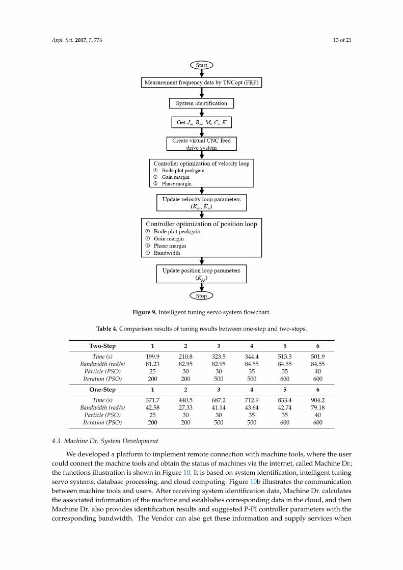
We developed a platform to implement remote connection with machine tools, where the usercould connect the machine tools and obtain the status of machines via the internet, called Machine Dr.;the functions illustration is shown in Figure 10. It is based on system identification, intelligent tuningservo systems, database processing, and cloud computing. Figure 10b illustrates the communicationbetween machine tools and users. After receiving system identification data, Machine Dr. calculatesthe associated information of the machine and establishes corresponding data in the cloud, and thenMachine Dr. also provides identification results and suggested P-PI controller parameters with thecorresponding bandwidth. The Vendor can also get these information and supply services when
Appl. Sci. 2017, 7, 776 14 of 21
needed. Thus, the vendor and users can reduce the maintenance duration and increase the efficiencyof the machine tools.
Appl. Sci. 2017, 7, 776 14 of 21
parameters with the corresponding bandwidth. The Vendor can also get these information and
supply services when needed. Thus, the vendor and users can reduce the maintenance duration and
increase the efficiency of the machine tools.
In addition, when the machine tools have already been in use for some time, and the stiffness of
the structure may have changed, Machine Dr. recommends suitable parameters to enhance the
bandwidth. Figure 11a shows the results of using the Machine Dr. The current system parameters
obtained by system identification are shown in the right column and the suggested controller
parameters are listed as below. Furthermore, Machine Dr. also provides the function of remote
monitoring, since communication has already been established between the user and the CNC
machine tools though the platform. When a user operates the software to survey the machine, the
information of the machine is stored in the cloud, which is shown in Figure 11b. As the result, both
the user and vendor can monitor the machine operation status, servo parameters, tuning history, etc.
by their personal computer (PC) remotely.
In summary, Machine Dr. combines cloud computing with knowledge of CNC machine tools to
develop additional features for CNC machine tools. Machine Dr. provides customers and vendors a
more easy method of controlling and obtaining information on machine tools. The vendor can also
receive these data from the platform. As the result, the vendor can keep track the condition of CNC
machine tools which are sold, and then services can be easily offered. In addition to this, if problems
occur with the machine tools, the vendor may obtain the causes of the problems from the data stored
in the cloud. Consequently, downtime and customers’ service time can be reduced.
(a)
(b)
Figure 10. Illustration of the cloud platform—Machine Dr. system; (a) functions illustration; (b)
communication between the user and the cloud servo system. Figure 10. Illustration of the cloud platform—Machine Dr. system; (a) functions illustration;(b) communication between the user and the cloud servo system.
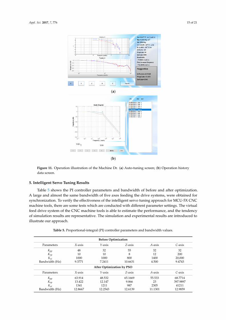
In addition, when the machine tools have already been in use for some time, and the stiffness of thestructure may have changed, Machine Dr. recommends suitable parameters to enhance the bandwidth.Figure 11a shows the results of using the Machine Dr. The current system parameters obtained bysystem identification are shown in the right column and the suggested controller parameters arelisted as below. Furthermore, Machine Dr. also provides the function of remote monitoring, sincecommunication has already been established between the user and the CNC machine tools though theplatform. When a user operates the software to survey the machine, the information of the machineis stored in the cloud, which is shown in Figure 11b. As the result, both the user and vendor canmonitor the machine operation status, servo parameters, tuning history, etc. by their personal computer(PC) remotely.
In summary, Machine Dr. combines cloud computing with knowledge of CNC machine tools todevelop additional features for CNC machine tools. Machine Dr. provides customers and vendors amore easy method of controlling and obtaining information on machine tools. The vendor can alsoreceive these data from the platform. As the result, the vendor can keep track the condition of CNCmachine tools which are sold, and then services can be easily offered. In addition to this, if problemsoccur with the machine tools, the vendor may obtain the causes of the problems from the data storedin the cloud. Consequently, downtime and customers’ service time can be reduced.
Appl. Sci. 2017, 7, 776 15 of 21Appl. Sci. 2017, 7, 776 15 of 21
(a)
(b)
Figure 11. Operation illustration of the Machine Dr. (a) Auto‐tuning screen; (b) Operation history data
screen.
5. Intelligent Servo Tuning Results
Table 5 shows the PI controller parameters and bandwidth of before and after optimization. A
large and almost the same bandwidth of five axes feeding the drive systems, were obtained for
synchronization. To verify the effectiveness of the intelligent servo tuning approach for MCU‐5X
CNC machine tools, there are some tests which are conducted with different parameter settings. The
virtual feed drive system of the CNC machine tools is able to estimate the performance, and the
tendency of simulation results are representative. The simulation and experimental results are
introduced to illustrate our approach.
Table 5. Proportional‐integral (PI) controller parameters and bandwidth values.
Before Optimization
Parameters X‐axis Y‐axis Z‐axis A‐axis C‐axis
Kpp 48 32 55 32 32
Kvp 10 10 8 12 200
Kvi 1000 1000 800 1400 20,000
Bandwidth (Hz) 9.3771 7.2411 10.6631 4.500 9.4743
After Optimization by PSO
Parameters X‐axis Y‐axis Z‐axis A‐axis C‐axis
Kpp 63.914 48.532 65.1669 55.533 68.7714 Kvp 13.422 12.147 9.866 23 397.9897 Kvi 1341 1211 987 2305 41211
Bandwidth (Hz) 12.8667 12.2543 12.6139 11.1301 12.9859
Figure 11. Operation illustration of the Machine Dr. (a) Auto-tuning screen; (b) Operation historydata screen.
5. Intelligent Servo Tuning Results
Table 5 shows the PI controller parameters and bandwidth of before and after optimization.A large and almost the same bandwidth of five axes feeding the drive systems, were obtained forsynchronization. To verify the effectiveness of the intelligent servo tuning approach for MCU-5X CNCmachine tools, there are some tests which are conducted with different parameter settings. The virtualfeed drive system of the CNC machine tools is able to estimate the performance, and the tendencyof simulation results are representative. The simulation and experimental results are introduced toillustrate our approach.
Table 5. Proportional-integral (PI) controller parameters and bandwidth values.
Before Optimization
Parameters X-axis Y-axis Z-axis A-axis C-axis
Kpp 48 32 55 32 32Kvp 10 10 8 12 200Kvi 1000 1000 800 1400 20,000
Bandwidth (Hz) 9.3771 7.2411 10.6631 4.500 9.4743
After Optimization by PSO
Parameters X-axis Y-axis Z-axis A-axis C-axis
Kpp 63.914 48.532 65.1669 55.533 68.7714Kvp 13.422 12.147 9.866 23 397.9897Kvi 1341 1211 987 2305 41211
Bandwidth (Hz) 12.8667 12.2543 12.6139 11.1301 12.9859
Appl. Sci. 2017, 7, 776 16 of 21
5.1. Simulation Results
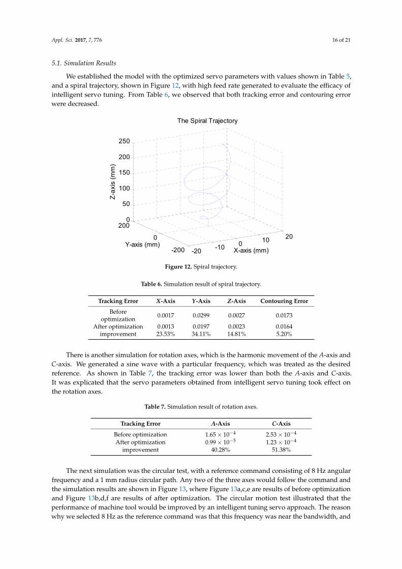
We established the model with the optimized servo parameters with values shown in Table 5,and a spiral trajectory, shown in Figure 12, with high feed rate generated to evaluate the efficacy ofintelligent servo tuning. From Table 6, we observed that both tracking error and contouring errorwere decreased.
Appl. Sci. 2017, 7, 776 16 of 21
5.1. Simulation Results
We established the model with the optimized servo parameters with values shown in Table 5,
and a spiral trajectory, shown in Figure 12, with high feed rate generated to evaluate the efficacy of
intelligent servo tuning. From Table 6, we observed that both tracking error and contouring error
were decreased.
There is another simulation for rotation axes, which is the harmonic movement of the A‐axis and
C‐axis. We generated a sine wave with a particular frequency, which was treated as the desired
reference. As shown in Table 7, the tracking error was lower than both the A‐axis and C‐axis. It was
explicated that the servo parameters obtained from intelligent servo tuning took effect on the rotation
axes.
Figure 12. Spiral trajectory.
Table 6. Simulation result of spiral trajectory.
Tracking Error X‐axis Y‐axis Z‐axis Contouring Error
Before optimization 0.0017 0.0299 0.0027 0.0173
After optimization 0.0013 0.0197 0.0023 0.0164
improvement 23.53% 34.11% 14.81% 5.20%
Table 7. Simulation result of rotation axes.
Tracking Error A‐axis C‐axis
Before optimization 1.65 10 2.53 10After optimization 0.99 10 1.23 10
improvement 40.28% 51.38%
The next simulation was the circular test, with a reference command consisting of 8 Hz angular
frequency and a 1 mm radius circular path. Any two of the three axes would follow the command
and the simulation results are shown in Figure 13, where Figure 13a,c,e are results of before
optimization and Figure 13b,d,f are results of after optimization. The circular motion test illustrated
that the performance of machine tool would be improved by an intelligent tuning servo approach.
The reason why we selected 8 Hz as the reference command was that this frequency was near the
bandwidth, and if the bandwidth increased, the system performance would be obviously improved.
Compared to the frequency within the bandwidth, the optimized FRF showed that 8 Hz had an
-20-10 0
10 20
-200
0
2000
50
100
150
200
250
X-axis (mm)
The Spiral Trajectory
Y-axis (mm)
Z-a
xis
(mm
)
Figure 12. Spiral trajectory.
Table 6. Simulation result of spiral trajectory.
Tracking Error X-Axis Y-Axis Z-Axis Contouring Error
Beforeoptimization 0.0017 0.0299 0.0027 0.0173
After optimization 0.0013 0.0197 0.0023 0.0164improvement 23.53% 34.11% 14.81% 5.20%
There is another simulation for rotation axes, which is the harmonic movement of the A-axis andC-axis. We generated a sine wave with a particular frequency, which was treated as the desiredreference. As shown in Table 7, the tracking error was lower than both the A-axis and C-axis.It was explicated that the servo parameters obtained from intelligent servo tuning took effect onthe rotation axes.
Table 7. Simulation result of rotation axes.
Tracking Error A-Axis C-Axis
Before optimization 1.65× 10⁻⁴ 2.53× 10⁻⁴
After optimization 0.99× 10⁻⁵ 1.23× 10⁻⁴
improvement 40.28% 51.38%
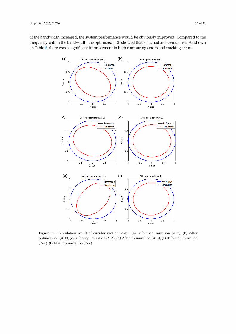
The next simulation was the circular test, with a reference command consisting of 8 Hz angularfrequency and a 1 mm radius circular path. Any two of the three axes would follow the command andthe simulation results are shown in Figure 13, where Figure 13a,c,e are results of before optimizationand Figure 13b,d,f are results of after optimization. The circular motion test illustrated that theperformance of machine tool would be improved by an intelligent tuning servo approach. The reasonwhy we selected 8 Hz as the reference command was that this frequency was near the bandwidth, and
Appl. Sci. 2017, 7, 776 17 of 21
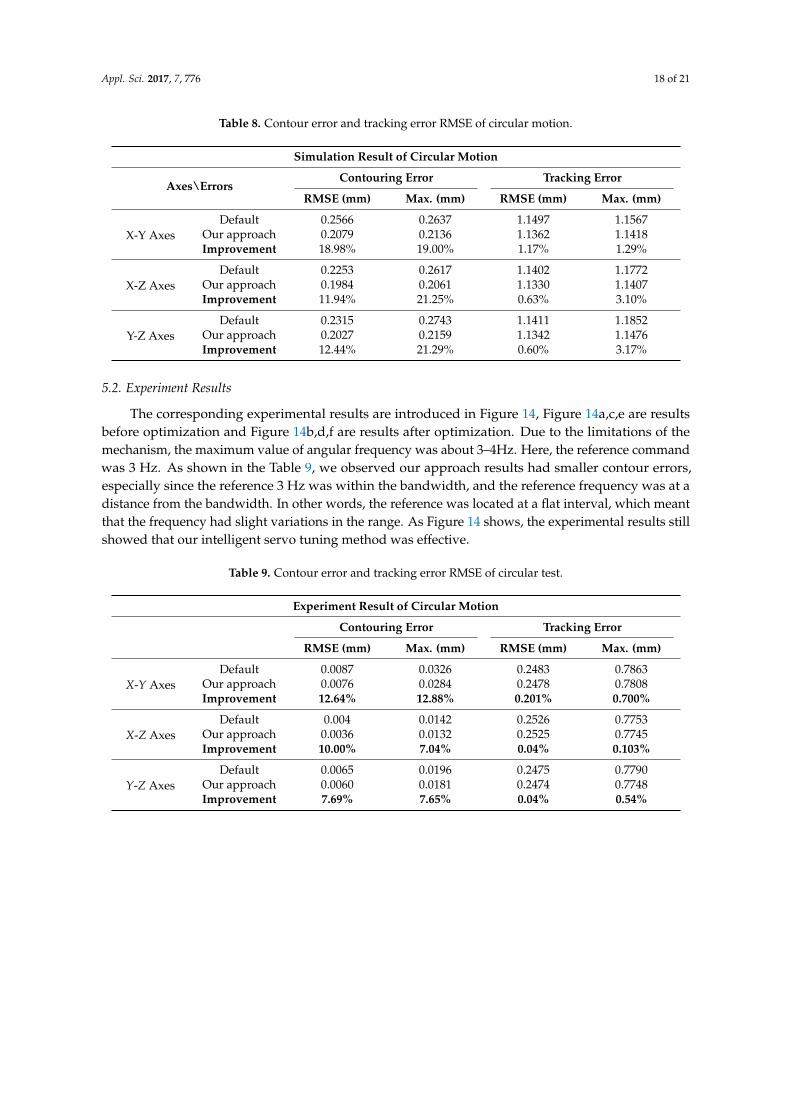
if the bandwidth increased, the system performance would be obviously improved. Compared to thefrequency within the bandwidth, the optimized FRF showed that 8 Hz had an obvious rise. As shownin Table 8, there was a significant improvement in both contouring errors and tracking errors.
Appl. Sci. 2017, 7, 776 17 of 21
obvious rise. As shown in Table 8, there was a significant improvement in both contouring errors and
tracking errors.
Figure 13. Simulation result of circular motion tests. Figure 13. Simulation result of circular motion tests. (a) Before optimization (X-Y), (b) Afteroptimization (X-Y), (c) Before optimization (X-Z), (d) After optimization (X-Z), (e) Before optimization(Y-Z), (f) After optimization (Y-Z).
Appl. Sci. 2017, 7, 776 18 of 21
Table 8. Contour error and tracking error RMSE of circular motion.
Simulation Result of Circular Motion
Axes\ErrorsContouring Error Tracking Error
RMSE (mm) Max. (mm) RMSE (mm) Max. (mm)
X-Y AxesDefault 0.2566 0.2637 1.1497 1.1567
Our approach 0.2079 0.2136 1.1362 1.1418Improvement 18.98% 19.00% 1.17% 1.29%
X-Z AxesDefault 0.2253 0.2617 1.1402 1.1772
Our approach 0.1984 0.2061 1.1330 1.1407Improvement 11.94% 21.25% 0.63% 3.10%
Y-Z AxesDefault 0.2315 0.2743 1.1411 1.1852
Our approach 0.2027 0.2159 1.1342 1.1476Improvement 12.44% 21.29% 0.60% 3.17%
5.2. Experiment Results
The corresponding experimental results are introduced in Figure 14, Figure 14a,c,e are resultsbefore optimization and Figure 14b,d,f are results after optimization. Due to the limitations of themechanism, the maximum value of angular frequency was about 3–4Hz. Here, the reference commandwas 3 Hz. As shown in the Table 9, we observed our approach results had smaller contour errors,especially since the reference 3 Hz was within the bandwidth, and the reference frequency was at adistance from the bandwidth. In other words, the reference was located at a flat interval, which meantthat the frequency had slight variations in the range. As Figure 14 shows, the experimental results stillshowed that our intelligent servo tuning method was effective.
Table 9. Contour error and tracking error RMSE of circular test.
Experiment Result of Circular Motion
Contouring Error Tracking Error
RMSE (mm) Max. (mm) RMSE (mm) Max. (mm)
X-Y AxesDefault 0.0087 0.0326 0.2483 0.7863
Our approach 0.0076 0.0284 0.2478 0.7808Improvement 12.64% 12.88% 0.201% 0.700%
X-Z AxesDefault 0.004 0.0142 0.2526 0.7753
Our approach 0.0036 0.0132 0.2525 0.7745Improvement 10.00% 7.04% 0.04% 0.103%
Y-Z AxesDefault 0.0065 0.0196 0.2475 0.7790
Our approach 0.0060 0.0181 0.2474 0.7748Improvement 7.69% 7.65% 0.04% 0.54%
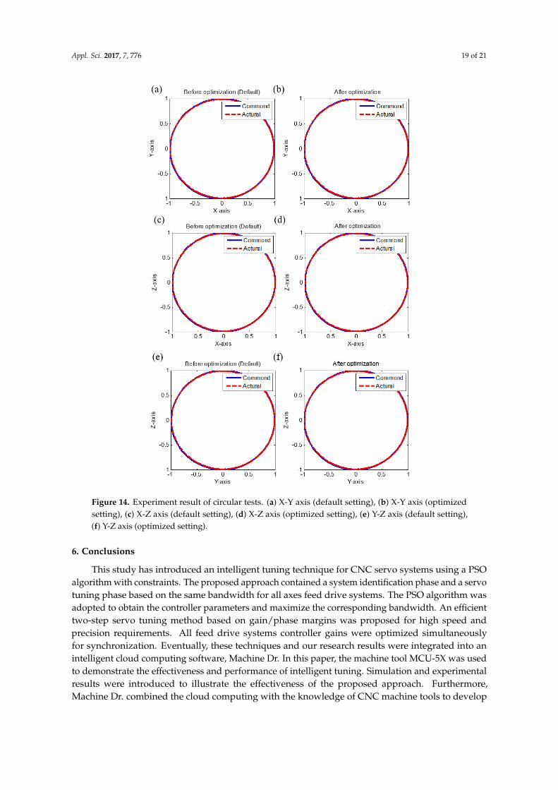
Appl. Sci. 2017, 7, 776 19 of 21Appl. Sci. 2017, 7, 776 19 of 21
Figure 14. Experiment result of circular tests. (a) X‐Y axis (default setting), (b) X‐Y axis (optimized
setting), (c) X‐Z axis (default setting), (d) X‐Z axis (optimized setting), (e) Y‐Z axis (default setting),
(f) Y‐Z axis (optimized setting).
6. Conclusions
This study has introduced an intelligent tuning technique for CNC servo systems using a PSO
algorithm with constraints. The proposed approach contained a system identification phase and a
servo tuning phase based on the same bandwidth for all axes feed drive systems. The PSO algorithm
was adopted to obtain the controller parameters and maximize the corresponding bandwidth. An
efficient two‐step servo tuning method based on gain/phase margins was proposed for high speed
and precision requirements. All feed drive systems controller gains were optimized simultaneously
for synchronization. Eventually, these techniques and our research results were integrated into an
intelligent cloud computing software, Machine Dr. In this paper, the machine tool MCU‐5X was used
to demonstrate the effectiveness and performance of intelligent tuning. Simulation and experimental
results were introduced to illustrate the effectiveness of the proposed approach. Furthermore,
Machine Dr. combined the cloud computing with the knowledge of CNC machine tools to develop
additional features for CNC machine tools. Machine Dr. provides customers and vendor with greater
ease of controlling and obtaining information on machine tools.
Figure 14. Experiment result of circular tests. (a) X-Y axis (default setting), (b) X-Y axis (optimizedsetting), (c) X-Z axis (default setting), (d) X-Z axis (optimized setting), (e) Y-Z axis (default setting),(f) Y-Z axis (optimized setting).
6. Conclusions
This study has introduced an intelligent tuning technique for CNC servo systems using a PSOalgorithm with constraints. The proposed approach contained a system identification phase and a servotuning phase based on the same bandwidth for all axes feed drive systems. The PSO algorithm wasadopted to obtain the controller parameters and maximize the corresponding bandwidth. An efficienttwo-step servo tuning method based on gain/phase margins was proposed for high speed andprecision requirements. All feed drive systems controller gains were optimized simultaneouslyfor synchronization. Eventually, these techniques and our research results were integrated into anintelligent cloud computing software, Machine Dr. In this paper, the machine tool MCU-5X was usedto demonstrate the effectiveness and performance of intelligent tuning. Simulation and experimentalresults were introduced to illustrate the effectiveness of the proposed approach. Furthermore,Machine Dr. combined the cloud computing with the knowledge of CNC machine tools to develop
Appl. Sci. 2017, 7, 776 20 of 21
additional features for CNC machine tools. Machine Dr. provides customers and vendor with greaterease of controlling and obtaining information on machine tools.
Acknowledgments: The authors would like to thank the reviewers for their suggestions. This researchwas supported by Ministry of Science and Technology, Taiwan grant to MOST-105-2218-E-005-005,MOST-106-2218-E-005-003, and MOST-105-2221-E-005-049-MY3.
Author Contributions: Chien-Yu Lin and Ching-Hung Lee initiated and developed the ideas related to thisresearch work. Both of them developed the presented novel methods, derived relevant formulations, and carriedout the performance analyses of simulation and experimental results. Chien-Yu Lin wrote the paper draft underChing-Hung Lee’s guidance and Professor Lee finalized the paper.
Conflicts of Interest: The authors declare no conflict of interest.
References
1. Srinivasan, K.; Tsao, T.C. Machine Tool Feed Drives and Their Control—A Survey of the State of the Art.J. Manuf. Sci. Eng. 1997, 119, 743–748. [CrossRef]
2. Khoshdarregi, M.R.; Altintas, Y. Contour error control of CNC machine tools with vibration avoidance.CIRP Ann. Manuf. Technol. 2012, 61, 335–338.
3. Koren, Y. Cross-coupled biaxial computer control for manufacturing system. J. Dyn. Syst. Meas. Control 1980,102, 265–272. [CrossRef]
4. Zaeh, M.F.; Kleinwort, R.; Fagerer, P.; Altintas, Y. Automatic tuning of active vibration control systems usinginertial actuators. CIRP Ann. Manuf. Technol. 2017. [CrossRef]
5. Altintas, Y.; Aslan, D. Integration of virtual and on-line machining process control and monitoring. CIRP Ann.Manuf. Technol. 2017. [CrossRef]
6. Altintas, Y. Virtual High Performance Machining. Procedia CIRP 2016, 46, 372–378. [CrossRef]7. Kilic, Z.M.; Altintas, Y. Generalized modelling of cutting tool geometries for unified process simulation.
Int. J. Mach. Tools Manuf. 2016, 104, 14–25. [CrossRef]8. Beudaert, X.; Mancisidor, I.; Ruiz, L.M.; Barrios, A.; Erkorkmaz, K.; Munoa, J. Analysis of the feed drives
control parameters on structural chatter vibrations. In Proceedings of the XIIIth International Conference onHigh Speed Machining (HSM2016), Nanjing, China, 18–20 October 2015.
9. Chauhan, V.; Patel, V.P. Multi-Motor sychronization techniques. Int. J. Sci. Eng. Technol. Res. 2014, 3, 319–322.10. Yao, W.S.; Yang, F.Y.; Tsai, M.C. Modeling and control of twin parallel-axis linear servo mechanisms for
high-speed machine tools. Int. J. Autom. Smart Technol. 2011, 1, 77–85. [CrossRef]11. Sencer, B.; Tajima, S. Frequency Optimal Feed Motion planning in computer numerical controller machine
tools for vibration avoidance. J. Manuf. Sci. Eng. 2017, 139. [CrossRef]12. Sencer, B.; Altintas, Y. Identification of 5-axis machine tools feed drive systems for contouring simulation.
Int. J. Autom. Technol. 2011, 5, 377–385. [CrossRef]13. Kima, M.S.; Chung, S.C. A systematic approach to design high-performance feed drive systems. Int. J. Mach.
Tools Manuf. 2005, 45, 1421–1435. [CrossRef]14. Wong, W.W.-S. Rapid Identification of virtual CNC drives. Master’s Thesis, University of Waterloo, Waterloo,
ON, Canada, 2007.15. Erkorkmaz, K.; Altintas, Y.; Yeung, C.H. Virtual computer numerical control system. CIRP Ann. 2006, 55,
399–402. [CrossRef]16. Altintas, Y.; Brecher, C.; Weck, M.; Witt, S. Virtual machine tool. CIRP Ann. 2005, 54, 115–138. [CrossRef]17. Lin, M.C. A Study of the CNC Parameter Tuning criteria according to the machining purposes. Master’s
Thesis, National Chung Hsing University, Kaohsiung, Taiwan, 2014.18. Chang, C.H. Study of virtual CNC servo control technology. Master’s Thesis, National Chung Hsing
University, Kaohsiung, Taiwan, 2014.19. Matsubara, A.; Kakino, Y; Sakurama, K. Design of linear motor servo systems under the influence of
structural vibrations. J. Jpn. Soc. Precis. Eng. 2000, 66, 122–126. [CrossRef]20. Kakino, Y.; Matsubara, A.; Li, Z.; Ueda, D.; Nakagawa, H.; Takeshita, T.; Maruyama, H. A study on total
tuning of feed drive systems of NC machine tools (2nd Report)—Single Axis Tuning. J. Jpn. Soc. Precis. Eng.1995, 61, 268–272. [CrossRef]
Appl. Sci. 2017, 7, 776 21 of 21
21. Matsubara, A.; Umemoto, M.; Tanaka, T.; Ibaraki, S.; Kakino, Y. Vibration analysis of feed drive systemsincluding base dynamics. In Proceedings of the 2002 Annual Meeting of JSPE Kansai Division, Osaka, Japan,5–7 August 2002.
22. Heidenhain. iTNC 530 HSCI—The Versatile Contouring Control for Milling, Drilling, Boring Machines andMachining Centers; Heidenhain Co.: Schaumburg, IL, USA, 2014; pp. 1–122.
23. Kennedy, J.; Eberhart, R.C. Particle swarm optimization. In Proceedings of the IEEE International Conferenceon Neural Networks, Perth, Australia, 27 November–1 December 1995; Volume 4, pp. 1942–1948.
24. Liang, J.H.; Lee, C.H. Efficient collision-free path-planning of multiple mobile robots system Using EfficientArtificial Bee Colony Algorithm. Adv. Eng. Softw. 2015, 79, 47–56. [CrossRef]
25. Lee, C.H.; Li, C.T.; Chang, F.Y. Species-based improved electromagnetism-like mechanism algorithm forTSK-type Interval-valued neural fuzzy system optimization. Fuzzy Sets Syst. 2011, 171, 22–43. [CrossRef]
26. Kuo, C.T.; Lee, C.H. Network-based type-2 fuzzy system with water flow like algorithm for systemidentification and signal processing. Smart Sci. 2015, 3, 21–34. [CrossRef]
27. Lee, C.H.; Lee, Y.C. Nonlinear systems design by a novel fuzzy neural system via hybridization of EM andPSO algorithms. Inf. Sci. 2012, 186, 59–81. [CrossRef]
28. Chao, C.T.; Sutarna, N.; Chiou, J.S.; Wang, C.J. Equivalence between fuzzy PID controllers and conventionalPID controllers. Appl. Sci. 2017, 7, 513. [CrossRef]
29. Chen, L.H.; Peng, C.C. Extended backstepping sliding controller design for chattering attenuation and itsapplication for servo motor control. Appl. Sci. 2017, 7, 220. [CrossRef]
30. Su, H.Y.; Hsu, Y.L.; Chen, Y.C. PSO-based voltage control strategy for loadability enhancement in smartpower grids. Appl. Sci. 2016, 6, 449. [CrossRef]
31. Yeung, C.H.; Altintas, Y.; Erkorkmaz, K. Virtual CNC system. Part I. System architecture. Int. J. Mach.Tools Manuf. 2006, 46, 1107–1123. [CrossRef]
32. Lee, K.; Ibaraki, S.; Matsubara, A.; Kakino, Y.; Suzuki, Y.; Arai, S.; Braasch, J. A servo parameter tuningmethod for high-speed nc machine tools based on contouring error measurement. Trans. Eng. Sci. 2003, 44,1–12.
33. Lee, W.H. Improvement of Contour Errors Using Cross-Coupled Control. Master’s Thesis, National SunYat-sen University, Kaohsiung, Taiwan, 2002.
© 2017 by the authors. Licensee MDPI, Basel, Switzerland. This article is an open accessarticle distributed under the terms and conditions of the Creative Commons Attribution(CC BY) license (http://creativecommons.org/licenses/by/4.0/).