Remote Sensing of Environment 129 (2013) 42–53

Contents lists available at SciVerse ScienceDirect

Remote Sensing of Environment

j ourna l homepage: www.e lsev ie r .com/ locate / rse

Urban growth of theWashington, D.C.–Baltimore, MDmetropolitan region from 1984to 2010 by annual, Landsat-based estimates of impervious cover

Joseph O. Sexton a,⁎, Xiao-Peng Song a, Chengquan Huang a, Saurabh Channan a,Matthew E. Baker b, John R. Townshend a

a Global Land Cover Facility, Department of Geographical Sciences, University of Maryland, 2181 LeFrak Hall, College Park, MD 20742, United Statesb Department of Geography and Environmental Systems, University of Maryland, Baltimore County, United States

⁎ Corresponding author. Tel.: +1 301 405 8165; fax:E-mail address: jsexton@umd.edu (J.O. Sexton).

0034-4257/$ – see front matter © 2012 Elsevier Inc. Allhttp://dx.doi.org/10.1016/j.rse.2012.10.025

a b s t r a c t

a r t i c l e i n f o

Article history:Received 13 April 2012Received in revised form 19 October 2012Accepted 27 October 2012Available online xxxx

Keywords:UrbanizationImpervious surfaceLand coverLandsatWashington, DCBaltimore, MDChesapeake Bay

Cities and surrounding suburbs are Earth's fastest growing land use. Urban impervious surfaces affect hy-drological and energy balances, as well as biological composition and functioning of ecosystems. Althoughdatasets have been produced documenting urban growth at multiple time periods in coarse intervals, thereremains an unmet need for observations spanning multiple decades at high frequency. We have developedan empirical method for retrieving annual, long-term continuous fields of impervious surface cover fromthe Landsat archive and applied it to the Washington, D.C.–Baltimore, MD megalopolis from 1984 to2010. Fitting and applying a single regression model over time, the method relies on a multi-annual train-ing sample of high-resolution impervious cover layers tied to coincident intra- and inter-annual Landsatimage composites. These predictor images are composited and normalized to maximize discriminationof impervious surfaces from intermittently bare agricultural fields and minimize inter-annual variationdue to phenology, solar illumination, and atmospheric noise. Excluding the year 2009 due to lack of dataavailability resulting from nearly continual winter snow cover, the resulting dataset is a continuous-fieldrepresentation of impervious surface cover at 30-m horizontal and annual temporal resolution from1984 to 2010. Average error was approximately ±6% cover, with outliers due to shadows from large build-ings in winter images. The region's impervious surface cover grew from 881 to 1176±11 km2 over the27-year span—an average annual gain of approximately 11±2 km2/year—with great variability amonglocal municipalities in terms of rate of development. Patterns including intensification (i.e., “infill”) andexpansion (i.e., exurban or “sprawl”) of development, as well as fragmentation and isolation of naturalareas were clearly visible in the data at various places and times. Neither impervious surface loss nordeceleration of growth were observed in any of the cities or counties over the study span. These findingsshow that empirical retrieval of impervious coverage at the spatial and temporal scale of the Landsatarchive is possible using dense time-stacks of calibrated Landsat images, and that long-term recordssuch as this can provide new opportunities for analyzing land-use patterns and their underlying causesto improve understanding of socio-economic processes and human–environment interactions.

© 2012 Elsevier Inc. All rights reserved.

1. Introduction

Although urban areas cover only 0.5% of Earth's terrestrial surface(Schneider et al., 2009), cities represent one of Earth's fastest growingland-use types on a per-area basis, and over half of the planet's 7 bil-lion humans now reside in cities (UNFPA, United Nations PopulationFund, 2011). A characteristic land cover and indicator of urban landuse is impervious surface cover, a category grouping all surface mate-rials through which precipitation does not penetrate, including pavedroads, sidewalks, parking lots, buildings, and other built structures.Urban impervious surfaces generate the “urban stream syndrome”(Walsh et al., 2005), which is characterized by increased hydroperiod

+1 301 314 9299.

rights reserved.

variability, water temperature, sediment load, and levels of heavymetals, nitrogen, phosphorous, and fecal coliform bacteria. Urbansurfaces also generate the “urban heat island effect” (Oke, 2006), anincrease in temperature due to shifting energy balance toward sensibleover latent heat fluxes that has been shown to alter regional climate,shift biotic community composition and even accelerate climate-induced species' range shifts (Menke et al., 2010). Urbanization is alsoassociated with the “demographic transition” in humans (Davis,1945), manifested by delayed reproduction and decreased birth anddeath rates leading to slower or even negative population growth rates.

Monitoring the spatio-temporal complexities of urbanization hasbeen difficult. Land-use dynamics exhibit temporal nonlinearity andspatial heterogeneity due to complex interactions with the socio-economic and ecological environment (Lambin et al., 2003). Urbaniza-tion is a feedback system that is economically driven, promoted by

Fig. 1. Study area. Counties labeled are those for which impervious surface referencedata were collected. The dotted line represents the nominal WRS-2 boundary, butthe shaded region indicates the effective study area, the intersection of all WRS-2 im-ages used.

43J.O. Sexton et al. / Remote Sensing of Environment 129 (2013) 42–53

local zoning and taxation policies, and constrained by laws to conservenatural resources and open spaces (Westervelt et al., 2011). In order tomonitor change and understand the causes and consequences of urban-ization, land-cover datasets must have sufficient temporal resolution torecord the complexities of change. Jensen and Cowen (1999) called for a1- to 5-year basis for monitoring urbanization, similar to the recom-mendation of Lunetta et al. (2004) of a 3-year frequency for monitoringchange in forests.

Impervious surfaces have been remotely sensed at a range of spatialscales using a variety of data sources and methods. Several global landcover datasets include urban categories (e.g., Friedl et al., 2002;Hansen et al., 2000; Loveland et al., 2000; Potere et al., 2009; Small etal., 2005), but the coarse resolution of such data sets is insufficient torepresent spatial variation within cities, towns, and settlements. Usingseasonal triplets of multi-spectral Landsat images, Yang et al. (2003)generated a percent impervious surface cover dataset for the 2001 Unit-ed States' National Land Cover Dataset ("NLCD 2001") (Homer et al.,2004) at 30-m resolution. Leveraging the distinct geometric patternsof anthropogenic structures, high-resolution (b5 m) data have beenused in manual digitization and automated image segmentation ap-proaches to detecting impervious cover (e.g., Goetz et al., 2003;Thomas et al., 2003). LightDetection AndRanging (LiDAR) andSyntheticAperture Radar (SAR) measurements of vertical structure are also in-creasingly being employed to detect urban and impervious types(Hodgson et al., 1999; Jiang et al., 2009).

Extension of impervious surface records into the temporal domainhas been more difficult, and so the great majority of impervious surfacedatasets currently record only one point in time. However, multi-temporal remote sensing of urban cover has had some recent successes,and development is acceleratingwith recent increases in data availability.Masek et al. (2000)monitored urbanization around theWashington, D.C.metropolitan area in two broad intervals between 1973 and 1996 bysubtracting NDVI images recorded by Landsat Multi-Spectral Scan-ner (MSS) and Thematic Mapper (TM) sensors. More recently, Yinet al. (2011) retrieved a time series of four maps between 1979 and2009 from Landsat data to observe long-term acceleration in thedevelopment of the Shanghai metropolitan area, and Taubenböcket al. (2012) combined Landsat images from circa 1975, 1990,2000, and 2010 and InSAR data from 2010 to monitor growth of 27megacities at an approximately decadal interval. Suarez-Rubio etal. (2012) employed spectral endmember analysis, decision trees,and post-classification morphological analysis to assess exurban de-velopment nearWashington, D.C. However, despite their advantagesover static maps, bi-temporal, and even coarsely multi-temporaldatasets do not have the necessary temporal scale to observehigher-order complexities (e.g., acceleration and deceleration) ofland-cover and land-use change. In order to resolve these patterns,observations must span multiple decades at high frequency.

In this paper, we describe an empirical method for retrievinglong-term records of impervious surface cover from time series ofLandsat images, using the rapidly growingWashington, D.C.–Baltimore,MD metropolitan area as an exemplar of a variety of change dynamics.We estimate the uncertainty of our results by validation relative to anindependent, withheld sub-sample of the reference data in multipleyears.We then highlight characteristic patterns and dynamics of urban-ization in the region, comparing our findings to previous studies in theregion based on other methods.

2. Methods

2.1. Study area

Our study area was the path-15/row-33 scene of the LandsatWorld Reference System 2 (WRS-2), encompassing the Washington,D.C.–Baltimore metropolitan region on the eastern seaboard of theUnited States (Fig. 1). The natural vegetation of the region consists

predominantly of mixed forests dominated by deciduous tree spe-cies. Land use in the region is mainly agricultural, with many smalltowns and a few large urban agglomerations around the anchor cit-ies of Washington, D.C. and Baltimore, Maryland. Although the re-gion is among the nation's fastest-growing in terms of humanpopulation, most growth has been outside of urban cores. For exam-ple, while the human population of Washington shrank from6.07×105 to 6.02×105 and that of Baltimore shrank from7.36×105 to 6.21×105 residents between 1990 and 2010, three out-lying Maryland counties—Calvert, Howard, and Montgomery—grewfrom 0.51×105, 1.87×105, and 7.57×105 residents in 1990 to0.89×105, 2.87×105, and 9.72×105 residents in 2010 respectively(Maryland State Archives, 2011; US Census Bureau, 2012).

2.2. Model

We modeled impervious surface cover (ISC), the percentage ofeach pixel covered by impervious surfaces, as a piecewise-linear func-tion of a set of predictors derived from multi-spectral measurements(X):

ISCi;t ¼ f Xi;t

� �;

where subscript i denotes the pixel's location in space and t refers toits location in time, indexed by year. By multiplying by the pixel's area(i.e., 900 m2), ISC may be converted to impervious surface cover, ISA,expressed in areal units. Derivation of the spectral predictors, X, isdescribed in the following section.

2.3. Data

Reference measurements of impervious cover were composed fromvector GIS layers of impervious surfaces acquired from local jurisdic-tions over multiple years. Predictor data were seasonal composites ofLandsat images. Between 1984 and 2010, every year was included inthe analysis except 2009, whichwas excluded due to insufficientwinterdata availability resulting from record snowstorms and nearly continualwinter snow cover.

2.3.1. Reference impervious dataImpervious surface data spanning multiple years were collected

from planimetric data recorded by municipalities within the study

44 J.O. Sexton et al. / Remote Sensing of Environment 129 (2013) 42–53

area. These data were provided by: Calvert and Howard counties, MDfor 2006; Carroll and St.Mary's counties,MD for 2007; andWashington,D.C. and Queen Anne's County, MD for 2008. Polygons surroundingroads, parking lots, buildings, driveways, and sidewalks using sub-meter resolution imagery were digitized by local municipalities.These data were generalized to a common binary pervious/imperviousscheme (including all of the above features as “impervious” and theexcluded “background” polygon assumed to be undeveloped, pervi-ous surface), transformed to a common geographic projection,rasterized to (binary) 1-m resolution, and resampled to continuous(percent-cover) scale at Landsat (30-m) resolution. Eighty-five per-cent of the ISC pixels were used as a training sample for model fitting,and the other 15% were randomly sampled and withheld as a testsample for validation.

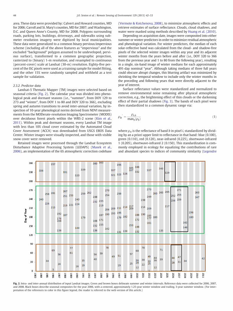
2.3.2. Predictor dataLandsat-5 Thematic Mapper (TM) images were selected based on

seasonal criteria (Fig. 2). The calendar year was divided into pheno-logical peak and dormant seasons (i.e., “summer”, from DOY 129 to273 and “winter”, from DOY 1 to 80 and DOY 320 to 366), excludingspring and autumn transitions to avoid inter-annual variation, by in-spection of 10-year phenological norms derived from NDVI measure-ments from the MODerate-resolution Imaging Spectrometer (MODIS)over deciduous forest pixels within the WRS-2 scene (Kim et al.,2011). Within peak and dormant seasons, every Landsat TM imagewith less than 10% cloud cover estimated by the Automated CloudCover Assessment (ACCA) was downloaded from USGS EROS DataCenter. Winter images were visually inspected, and those with visiblesnow cover were removed.

Retained images were processed through the Landsat EcosystemDisturbance Adaptive Processing System (LEDAPS) (Masek et al.,2006), an implementation of the 6S atmospheric correction codebase

Fig. 2. Intra- and inter-annual distribution of input Landsat images. Green and brown boxesand 2008. Black boxes describe seasonal composites for the year 2006, with a centered, apppretation of the references to color in this figure legend, the reader is referred to the web v

(Vermote & Kotchenova, 2008), to minimize atmospheric effects andretrieve estimates of surface reflectance. Clouds, cloud shadows, andwater were masked using methods described by Huang et al. (2010).

Depending on acquisition date, images were composited into eithersummer orwinter predictors in order tominimize residual atmosphericand phenological variation. For winter predictors, the median of eachsolar-reflective band was calculated from the cloud- and shadow-freepixels of the selected winter images within any year and its adjacentwinter months from the years before and after (i.e., DOY 320 to 366from the previous year and 1 to 80 from the following year), resultingin a single, six-band image of winter medians for each approximately491-day nominal “year”. Although taking medians of three full yearscould obscure abrupt changes, this blurring artifact was minimized byshrinking the temporal window to include only the winter months inthe preceding and following years that were directly adjacent to theyear of interest.

Surface reflectance values were standardized and normalized toremove environmental noise remaining after physical atmosphericcorrection, e.g., the brightening effect of thin clouds or the darkeningeffect of their partial shadows (Fig. 3). The bands of each pixel werethen standardized to a common dynamic range via:

ρib′ ¼ ρx;b

maxb ρbð Þ ð1Þ

where ρxi is the reflectance of band b in pixel i, standardized by divid-ing by an a priori upper limit to reflectance in that band: blue (0.100),green (0.110), red (0.120), near-infrared (0.225), shortwave-infrared1 (0.205), shortwave-infrared 2 (0.150). This standardization is com-monly employed in ecology for equalizing the contributions of rareand abundant species to indices of community similarity (Legendre

delineate summer and winter intervals. Reference data were collected for 2006, 2007,roximately 1.25-year winter window and trailing, 3-year summer window. (For inter-ersion of this article.)

Fig. 3. Winter-median surface reflectance values over time for selected stable pixels of representative land cover types within the study area. Missing values over Baltimore andwater are due to clouds. Note the synchronicity of fluctuations between bands in comparison to the stability of NDVI over time (NDVI has been rescaled by a factor of 1000 for com-parison.) (For interpretation of the references to color in this figure legend, the reader is referred to the web version of this article.)

45J.O. Sexton et al. / Remote Sensing of Environment 129 (2013) 42–53

& Legendre, 1998). Standardized reflectances were then normalizedby dividing by their across-band sum in each pixel:

ρi;b′′ ¼ ρ′

i;b

∑iρ′i;b: ð2Þ

This process operated at the pixel level and satisfactorily reducedinter-annual variations that were correlated across all bands (Fig. 4).

The normalized winter medians were augmented with informa-tion from the growing season to maximize discrimination betweenintermittently bare agricultural fields and persistently bare impervi-ous surfaces. The Normalized Difference Vegetation Index (NDVI)was calculated from summer images, and then each summer NDVIpixel was subjected to a three-year (summer) trailing-maximumconvolution:

sNDVIi ¼ maxtþ2t NDVIið Þ ð3Þ

in which the maximum NDVI value is taken for each pixel in summerimages of the nominal year and the two years following. This processconsistently minimized year-to-year phenological differences andamplified the difference between vegetated and unvegetated surfacesacross urban, suburban, and agricultural land uses (Fig. 5).

2.4. Modeling

Impervious surface layers were overlaid on seasonal Landsat mea-surements from coincident years, and a joint sample of reference andpredictor variables was extracted to generate a multi-year trainingdataset (n=2,178,175). The training data were used to fit a regres-sion tree (Cubist™; Quinlan, 1993) to infer impervious surface coverfrom the winter median reflectances and summer maximum NDVI.The fitted model was applied to every year's two-season Landsatdata from 1984 to 2010 to retrieve annual estimates of impervioussurface cover. Impervious cover of pixels missing reflectance data inone season (e.g., due to cloud cover) was estimated based on avail-able data from the other season.

2.5. Validation

Errors were evaluated relative to the training data by ten-foldcross validation and also to the ~15% withheld (i.e., not included intraining) sub-sample of the reference data for model testing (n=396,751). Ten-fold cross validation is a procedure in which themean value of a selected metric is calculated based on ten randomsubsets of the original data; the data are split into 10 randomsub-sets, a model fit to 90% of the data is validated against eachremaining 10% in iteration across the ten subsets, and the mean is

Fig. 4. Standardized and normalizedwinter-median surface reflectance values over time for forest, high-density urban, and low-density urban pixels. Note the stability of the values com-pared to the untransformed data in the previous figure. (For interpretation of the references to color in this figure legend, the reader is referred to the web version of this article.)

46 J.O. Sexton et al. / Remote Sensing of Environment 129 (2013) 42–53

calculated from the ten sub-sample evaluations. Cross-validation wasperformed primarily for the purposes of model development, whereasvalidation based on the withheld sample was used for estimationand characterization of errors. Uncertainty metrics were based onaverage differences between paired model and reference values,quantified by Mean Bias Error (MBE), Mean Absolute Error (MAE),and Root-Mean-Squared Difference (RMSD):

MBE ¼ ∑ni¼1

Mi−Ri

nð4Þ

MAE ¼ ∑ni¼1

Mi−Rij jn

ð5Þ

RMSD ¼ffiffiffiffiffiffiffiffiffiffiffiffiffiffiffiffiffiffiffiffiffiffiffiffiffiffiffiffiffiffiffiffiffi∑n

i¼1 Mi−Rið Þ2n

sð6Þ

where Mi and Ri are respectively modeled and reference imperviouscover values at a location i in a sample of size n.

3. Results

3.1. Model fit and validation

Internal cross-validation of the regression tree estimated an averageerror (MAE) of ±5.9% cover, with a correlation coefficient between

inferred and observed cover of 0.64. Estimates were constrained to liewithin the interval of 0–100% cover, so errors were predominantly pos-itive at low impervious cover and negative at high cover. Results wereidentical for training and withheld test data, suggesting negligiblemodel over-fittingwithin the sample relative to the population. All vari-ables were used with approximately equal frequency in terminal-noderegressions, but summer-maximum NDVI was by far the most impor-tant predictor in terms of usage rate in conditional splits (Table 1).Winter-median blue, SWIR2, and red reflectances were each usedin approximately half of tree splits, whereas winter-median SWIR1,green, and NIR reflectances were relatively unimportant in definingtree splits.

Differences between estimated and reference values of percent im-pervious cover had a strongly peaked distribution centered close tozero (Fig. 6). The average difference between model and referencecover (Mean Bias Error, MBE) was −3.5%, with a median of 0.0. Theskew was due to a small mode of large, negative errors located at ap-proximately 100% cover in the reference data, which further inspectionrevealed to be under-estimation of impervious cover in the shadows oftall buildings — an artifact imposed by the shallow illumination anglesof winter images. Another source of under-estimation was the obscur-ing of roads, sidewalks, and other short-statured structures by trees —an artifact which was partially, but not completely, minimized byusing dormant-season images. Over-estimates tended to be small, fol-lowing an approximately negative-exponential distribution, whereasunder-estimates were more normally and widely distributed. MAE of

Fig. 5. Demonstration of 3-year, summer-maximum NDVI in urban (Washington, D.C.), suburban (Northern Virginia), and agricultural (Delmarva Peninsula, Maryland) regions.

47J.O. Sexton et al. / Remote Sensing of Environment 129 (2013) 42–53

independent test data was 5.87%, equal to that obtained from cross-validation. RMSDwasmuchhigher, 14.46%, corroborating the strong in-fluence of outliers. The correlation coefficient (r) between estimated

Table 1Cubist™ regression tree summary of predictor variable importance.

Predictor layer Condition (split) use rate Terminal-node regressionuse rate

Summer-maximum NDVI 0.82 0.82Blue 0.55 0.76SWIR2 0.54 0.83Red 0.48 0.73SWIR1 0.13 0.80Green 0.11 0.75NIR 0.05 0.71

and reference impervious cover was 0.64, again likely due to the lever-age of outliers on the negative tail of the error distribution.

Although uncertainty increased in proportion to area, local dynam-icswere capturedwith high certainty. This local precision is exemplifiedby the development of FedEx Field, a sports stadium in Landover, PrinceGeorge's County, Maryland (Fig. 7). Impervious surfaces that remainedconstant at or near zero cover values in all three image dates (1993,2001, and 2010) are black — e.g., the large patches of forest and fieldsin the western and northeastern portions of the image. Patches thatremained at or near complete (100%) impervious cover in all threeyears—e.g., the numerous large roads and commercial parcels through-out the image—are white. Patches with constant values between 0 and100% range in various shades of gray — e.g., the curving residentialstreets, which exhibit an erroneous bluish tint due to the filling in of

Fig. 6. Distribution of error in estimates of percent impervious surface cover relative toa random 15% sub-sample of reference data withheld for validation. Data are from apooled sample from several municipalities over three years.

Fig. 7. Development of FedEx Field (Landover, MD) and surrounding neighborhoods.The temporal composite (bottom) shows impervious cover in 1993 in blue, 2001 ingreen, and 2010 in red. White pixels were impervious in all three dates, and blackpixels were non-impervious in all three dates. Pixels that were impervious in both2001 and 2010 but not in 1993 are displayed in yellow (e.g., FedEx Field, near the cen-ter of image), and pixels that were impervious in 1993 and 2001 but not 2010 are incyan (e.g., demolished building in northwest corner of image). Pixels that were becameimpervious between 2001 and 2010 are red — e.g., the residential subdivision in thenortheast corner of the image.

48 J.O. Sexton et al. / Remote Sensing of Environment 129 (2013) 42–53

landscape trees overmultiple decades. Patches thatwere developed be-tween 1993 and 2001 and remained so in 2010 are yellow— e.g., FedExField, slightly below and right of center in the image, was built in 1997.Note the elliptical patch of zero-impervious cover in the center of thestadium; this is the grass playing field. Patches that were developed be-tween 2001 and 2010 are red— e.g., the commercial–residential devel-opment in the northeast corner of the image (Note that development iscaptured reliably regardless of whether the preceding land cover wasforest or herbaceous agriculture.). The cyan patch in the northwest cor-ner of the image is an exceedingly rare class of urban change: impervi-ous surface loss, which can be confirmed as buildings in 1993 and 2001but bare, disturbed soil in 2010.

3.2. Impervious surface development of the Washington, D.C.–Baltimore,MD region

In 1984, the region had approximately 88,129±1135 ha of impervi-ous surface cover — 0.037±0.0012% of the total area. In 2010, theregion's impervious cover had grown to approximately 117,646 ha ofimpervious surface (4.9% of the total area). The average annual rate ofgrowth was 1135±208 ha/year (Pb0.0001) — i.e., approximately 11km2 of new impervious surfaces gained per year over the region. Thedistribution of impervious surface in 1984 shows the two major citiesof the region—Washington, D.C. and Baltimore, MD—as hotspots ofimpervious cover linked by a suburban corridor served by rail and anumber of arterial roads, including Interstate highway I-95, US highwayUS-29, andMaryland State Route-2 (Fig. 8). Richmond, Virginia lieswellto the south, connected toWashington, D.C. by I-95. Annapolis, MD, thestate capital, is also visible as a small cluster of impervious surface southof Baltimore and East of Washington, D.C. on the Chesapeake Bay andconnected to Washington by US Highway 50 and to Baltimore by I-97,which was completed in 1993. The heavily industrialized Baltimorehas a greater density of impervious surface than the more residentialcities, Washington and Annapolis, whose principal economies aregovernance. Several smaller cities and towns are also visible as clustersof impervious surface between Washington and Baltimore, inter-connected by a lattice of arterial highways and smaller roads. ThePatuxent Wildlife Research Refuge, which is covered predominantlyby forests, fields, and natural wetlands, is a large patch of persistentnon-impervious cover between 1984 and 2010 within the suburbanD.C.–Baltimore corridor. Likewise, agricultural lands are visible aslarge regions of low impervious cover outside the greater metropolitan

area (e.g., northwest corner of the study area, southeast of Washington,and east of the Chesapeake Bay).

By 2010, the impervious surface of the small towns betweenWashington and Baltimore—aswell as that ofWashington and Baltimorethemselves—had intensified and expanded. Infill development is ap-parent as intensification of increasing imperviousness within the cit-ies. Road widening is also visible, e.g., as an increase in impervioussurface percentage of the US-50 roadway. Fragmentation and isola-tion of natural forest habitat are apparent as increases of impervioussurfaces abutting and surrounding the wildlife refuge and otherareas.

Fig. 8. Impervious surface cover of the study area in 1984, and growth of the D.C.–Baltimore corridor from 1984 to 2010. Points of interest are: (A) Washington, D.C.; (B) Baltimore,Maryland; (C) Annapolis, Maryland; (D) Patuxent Wildlife Research Refuge; and (E) US Highway 50. Note that the data displayed are from years without training data.

49J.O. Sexton et al. / Remote Sensing of Environment 129 (2013) 42–53

Linear growth is observable in several of the region's municipalities(Fig. 9, Table 2). Fairfax county showed the greatest increase in imper-vious area, at a rate of 163.91±21.67 ha/year, or 0.16±0.021% of thecounty area per year (pb0.001). Calvert county developed much moreslowly, at a rate of 11.52±4.56 ha, or 0.02±0.008%, per year (p=0.019). Howard county's impervious surface cover nearly doubled inarea, increasing at a rate of 65.29±7.08 ha (0.1±0.01%) per year, andthat of Prince George's County, MD increased at a rate of 108.22±24.5 ha (0.09±0.02%) per year. However, given the small proportionof change over the large areas of the counties, precisionwas insufficientto consistently observe second-order changes such as acceleration ordeceleration. Uncertainty in impervious surface cover increased witharea, so the temporal trajectories of the larger counties—e.g., PrinceGeorge's County, MD and Fairfax County, VA—are surrounded by greaternoise than are the smaller Howard and Calvert Counties, MD. However,this variation is consistent with overall error estimates.

Although lying in different states and therefore different taxationand zoning policies, Fairfax and Prince George's counties shared similargrowth patterns: low to intermediate fractional cover, high areal cover,and rapid development over the study span — suggesting that theirother similarities (e.g., large, suburban, and close to the District ofColumbia) have a greater effect on development than local land-usepolicies. Their large size and large proportion of intermediate covervalues also likely led to their relatively large uncertainties.

Cities were proportionally more developed than counties (Fig. 9),with Baltimore, MD, Alexandria, VA, andWashington, D.C. themost de-veloped municipalities in the region. Cities showed great variability indevelopment rates, both amongmunicipalities andwithin somemunic-ipalities over time. In general, impervious surface growth in cities wasinversely proportional to existing impervious surface cover. The larger,

more developed cities of Baltimore and Washington, D.C. began withhigher proportional coverage and showed very little change over theperiod of study. In contrast, Manassas Park, VA began with a low pro-portion of impervious cover (~8%), but accelerated developmentaround 1995, shifting from growth of approximately 4% from 1984 to1995 (~0.3%/year) to nearly 0.6%/year from 1995 to 2010 (Fig. 9). Al-though the impervious cover of Fairfax city grew at a slow pace be-tween 1984 and 2010, that of Fairfax County grew much morequickly, indicating exurban, or “sprawl” development. Similarly, Freder-icksburg, VA accelerated its rate of development around the same time,shifting from near zero growth from 1984 to 1995 to approximately0.3% areal increase per year from 1995 to 2010. However, even giventhe clear growth of small cities such as these, much of Fredericksburg'sdevelopment was outside its municipal boundaries (Fig. 10).

4. Discussion

4.1. Urban growth of the Washington, D.C.–Baltimore, MD metropolitanregion

TheWashington, D.C. metropolitan area and the greater ChesapeakeBay watershed have received much attention due to their rapid de-velopment and ecological importance. Masek et al. (2000) used dif-ferences in NDVI in two intervals (i.e., between three image dates)from 1973 to 1996 to detect changes in urban cover in theWashington,D.C. metropolitan area. Jantz et al. (2005) assessed the loss of resourcelands in the broader Chesapeake Bay watershed between 1990 and2000 by overlaying a discretized map of impervious cover changefrom 1990 and 2000 on land cover maps from circa 1990. Suarez-Rubio et al. (2012) assessed exurban development in northern Virginia

Fig. 9. Estimated change in impervious surface coverage of selected counties (top) and cities (bottom) from 1984 to 2010. No impervious cover map was possible for 2009, due tolack of winter data availability from major snowstorms in 2009 and early 2010. Solid lines represent linear models for each municipality.

50 J.O. Sexton et al. / Remote Sensing of Environment 129 (2013) 42–53

and western Maryland between categorical maps from 1986, 1993,2000, and 2009.

The areas of interest of these studies all differ, and each studyresponded to the uncertainty of its urban cover estimates by coarseningthe thematic resolution to broad categories. However, some similaritiesare evident despite the differences in spatial and thematic scale. Overall,urban land cover increased at a rapid and accelerating pace in the re-gion, with growth concentrated at the expanding fringes of existingurban clusters. Growth in counties neighboring cities exceeded that ofoutlying counties as well as the cities themselves, reflecting a predom-inance of low-density development. Development patterns variedacross jurisdictions, with some counties adopting clustered patterns(e.g., Montgomery County, MD) and others adopting more dispersedpatterns of sprawl (e.g., Fairfax and Louden counties, VA).

Although all these studies are in agreement over the general spa-tial patterns and temporal trajectories of urbanization in the region,one important difference is evident between previous studies andour own. Masek et al. (2000) found an increase in built-up area of22 km2/year, Jantz et al. (2005) found a 41% increase in impervioussurface area over the entire watershed (most of which is less devel-oped than the Washington–Baltimore area), and Suarez-Rubio et al.

(2012) found an increase of 6.1%/year growth in exurban develop-ment alone. In contrast, our estimate based on per-pixel percentagesof impervious cover (~11 km2/year) is much more conservative thanany of these findings based on categorized data. Because urbanizationin the region is dominated by sparse development, our estimate,which is based upon data of higher thematic resolution, should beconsidered a refinement of these earlier estimates.

4.2. Long-term retrieval of impervious surface cover from the Landsatarchive

In a recent review of remote sensing methods for estimating im-pervious surface cover, Weng (2012) called for more research in thechange and evolution of impervious surfaces over time. The reviewfocused on novel machine learning algorithms and new data sources,concluding that high-resolution, SAR, LiDAR, and other new imageproducts can increase accuracy of maps of present and recent condi-tions. However, these new datasets do not have the spatial coverageor temporal scale needed to monitor urbanization over the long term.

The Landsat series of sensors, spanning over thirty years of Earth'sdynamic recent history, is unique in its ability to support retrieval of

Table 2Summary of regression coefficients and fit of linear regression of impervious surface area (ha) and cover (percent of municipal area) over time (years) from 1984 to 2010, excluding2009 (n=26, d.f.=24) for selected counties and cities. Cities and counties in bold font are mentioned in text.

Intercepta Slope

Municipality ha (S.E.) % (S.E.) P (>|t|) ha/year (S.E.) %/year (S.E.) P (>|t|) R2

Washington 4934 (96) 30.63 (0.59) 0.000 23.9 (6.5) 0.15 (3.65) 0.001 0.357Anne Arundel County 7365 (307) 6.83 (0.29) 0.000 75.5 (21.0) 0.070 (0.02) 0.001 0.350Baltimore 8274 (153) 39.25 (0.73) 0.000 11.7 (10.5) 0.06 (0.05) 0.275 0.049Calvert County 933 (67) 1.65 (0.12) 0.000 11.5 (4.6) 0.02 (0.01) 0.019 0.210Charles County 1861 (143) 1.56 (0.12) 0.000 32.7 (9.8) 0.03 (0.01) 0.003 0.318Howard County 2666 (104) 4.06 (0.16) 0.000 65.3 (7.1) 0.10 (0.01) 0.000 0.780Montgomery Countyb 7034 (257) 5.46 (0.20) 0.000 91.7 (17.6) 0.07 (0.01) 0.000 0.531Prince George's County 9485 (359) 7.51 (0.28) 0.000 108.2 (24.5) 0.09 (0.02) 0.000 0.448St. Mary's County 2163 (139) 2.27 (0.15) 0.000 −1.5 (9.5) −0.000 (0.01) 0.877 0.001Arlington 1707 (50) 25.23 (0.74) 0.000 6.0 (3.4) 0.09 (0.05) 0.090 0.115Alexandria 1288 (32) 32.80 (0.82) 0.000 1.2 (2.2) 0.03 (0.06) 0.586 0.013Fairfax 330 (10) 20.06 (0.59) 0.000 2.4 (0.6) 0.15 (0.04) 0.001 0.352Fairfax County 8694 (317) 8.45 (0.31) 0.000 163.9 (21.7) 0.16 (0.02) 0.000 0.704Falls Church 100 (4) 19.38 (0.76) 0.000 0.7 (0.3) 0.13 (0.05) 0.021 0.203Fredericksburg 311 (14) 11.39 (0.53) 0.000 8.5 (1.0) 0.31 (0.04) 0.000 0.755King George County 454 (38) 0.95 (0.08) 0.000 5.9 (2.623) 0.01 (0.01) 0.034 0.174Manassas 450 (18) 17.38 (0.68) 0.000 11.2 (1.2) 0.43 (0.05) 0.000 0.781Manassas Park 58 (4) 9.04 (0.59) 0.000 4.6 (0.3) 0.72 (0.04) 0.000 0.930Stafford County 971 (85) 1.37 (0.12) 0.000 36.8 (5.8) 0.05 (0.01) 0.000 0.629

a Years are adjusted so that the intercept is estimated at year 1984.b Partial coverage in study area.

51J.O. Sexton et al. / Remote Sensing of Environment 129 (2013) 42–53

land cover change records over long time scales (Goward et al., 2006;Gutman & Masek, 2012). However, fitting individual models for eachplace and time is simply too inefficient (and demanding of oftennon-existent archival reference data) for long-term retrievals. Alter-natively, extrapolation of robust models based on physically or statis-tically normalized imagery is a much more practical approach forextracting information from the full spatial and temporal extent ofthe Landsat archive. Whereas most algorithm development to datehas focused on maximizing accuracy in relatively few points in timeso that traditional change detection methods may be employed, ourregression-based approach allowed continuous-field estimation andstatistical inference using nearly every year in a twenty-seven yearspan.

Several factors enable use of Landsat data for long-term monitor-ing of impervious surface dynamics. Of primary importance is theUnited States' open-access data policy begun in 2009. Without inex-pensive (or free) data, impervious and other land cover mapping ef-forts would not have access to sufficient data volumes to fill cloudgaps or remove phenological and atmospheric noise by high-volumeimage compositing. Secondarily, reliable radiometric calibration, at-mospheric correction, and phenological selection are required forconsistent extrapolation of models to locations and times not sam-pled by reference data (Masek et al., 2006). Also, recent developmentof image compositing techniques for Landsat data (e.g., Huang et al.,2009a, 2009b; Roy et al., 2010) are necessary to dampen remnantnoise and identify the spectral and temporal signatures of imperviousor other surface materials.

The potential temporal domain of the specificmethod demonstratedhere is the era of Landsat-5 and Landsat-7 (i.e., from 1984 to the pres-ent). With wider uncertainties, extension back to 1972 might be possi-ble where sufficient Multi-Spectral Scanner (MSS) data are available(and similarly forward to newer sensors), although methods must bedeveloped to extrapolatemodels between sensors. Due to themethod'sreliance on the phenological discrimination of impervious surfaces, thepotential spatial domain of the method is confined to humid temperatebiomes, where rapid vegetation regrowth distinguishes intermittentlybare soil frompersistently bare urban surfaces. The approach is less like-ly to provide accuracy in arid, alpine, or otherwise sparsely vegetatedregions. Ultimately, however, this—and any other—empirical methodrequires high-quality reference data with adequate sampling overspace and time to represent the range of conditions within the domain

of extrapolation. For this, there is no better source of information thanthemunicipalities who record impervious surface coverage for the pur-poses of storm-water management and taxation.

The primary impediment to observing rapid changes in our timeseries was imprecision of impervious cover estimates in the temporaldimension. Although the pattern of cover was consistent across spacein any year, temporal trajectories of cover in any selected regionexhibited oscillations that cannot plausibly be attributed to realchange (Fig. 9). These errors could be reduced statistically, by increas-ing sampling of training data in the temporal domain, removing noisefrom the estimates and increasing model variance. However, giventhe consistency of the oscillation, there is likely a physical explanationfor the phenomenon. Landsat-5 orbited on a cycle repeating approx-imately every six years (not including adjustments), similar to thefrequency of the observed oscillation. This suggests the possibility ofBidirectional Distribution Function (BRDF) effects. BRDF effects havebeen observed in Landsat across space (Danaher et al., 2001), butonly recently have the data become sufficient to detect BRDF effectsover time. To ensure the precision of Landsat measurements in timeas well as space, this is an area of research which should be explored.

Remaining uncertainty notwithstanding, the multi-temporal accu-racies yielded by temporal compositing in this study are comparableto those reported for static and coarse time-serial maps in similar envi-ronments (Jiang et al., 2009; Yang et al., 2003, 2009). However, someknown challenges still remain. These include: generalization of rulesfor phenological selection and compositing of images, analysis and pre-diction of errors in locations and years not sampledwith reference data,and development of change-detection methodologies that make use ofboth continuous-scale data and estimates of uncertainty. Similar issueschallenge efforts to monitor forest cover (e.g., Hansen et al., 2010;Huang et al., 2009a, 2009b; Kennedy et al., 2010; Sexton et al., 2013;Townshend et al., 2012), and so there is much room formutual learningand advancement between these closely related fields of study.

4.3. A call for long-term, consistent records of land-cover change

Long-term records of impervious surface cover have great potentialfor application among urban growthmodelers andmanagers of policiesgoverning land-use change, as well as ecologists, hydrologists, andeconomists studying the effects of urbanization on physical, biological,and socio-economic systems. Rich in theory but relatively poor in

Fig. 10. Impervious surface development of Fredericksburg, VA from 1985 to 2010. Thecirca-2010 municipal boundary is outlined in white. Note that reference data were notavailable either within the spatial extent or any of the years presented.

52 J.O. Sexton et al. / Remote Sensing of Environment 129 (2013) 42–53

data, each of these groups is currently forced to base inference onuni-temporal, or at best coarsely multi-temporal, databases. In the so-cial sciences, inferences are commonly drawn by comparing a few, in-tensively studied case studies representing different scenarios (Turneret al., 2007), and similar limitations underlie the “space-for-time substi-tution” commonly employed in ecology (Pickett, 1989) and “paired

watershed” studies in hydrology. Although recent studies based onmulti-temporal landcover maps have shown accelerating rates andshifting patterns of development (e.g., Whitehurst et al., 2009; Yin etal., 2011)—patterns that require at least three observations in time—there are currently no consistent long-term records of land cover tosupport more powerful inferential approaches.

Efforts to produce the needed datasets, primarily in the area offorest-cover change, are now underway (Cohen et al., 2010; Huanget al., 2009a, 2009b; Kennedy et al., 2010). As these data improve,their primary use will likely continue to be for simple inventories ofland cover change, but their denser (i.e., ~annual) temporal samplingwill increase scientists' ability to observe the complexities of coupledhuman–natural systems. This will certainly precipitate more sophisti-cated socio-economic and ecological models, tighter correlation withother spatio-temporal datasets, and ultimately greater understandingand management of coupled human–natural systems. Already, agrowing number of social scientists, ecologists, and physicists are co-ordinating their efforts to better understand these systems (Daily &Matson, 2008), and it is the responsibility of the remote sensing com-munity to provide them with the long-term, consistent records need-ed for progress.

5. Conclusion

We have developed a method for retrieving retrospective continu-ous fields of impervious surface cover at 30-m spatial resolution andannual interval from the Landsat-5 archive, from approximately 1984to 2010. Our results depict the heterogeneous and nonlinear growthof impervious surfaces among the municipalities of the Washington,D.C.–Baltimore, MD metropolitan region, corroborating and refiningthe spatial, temporal, and thematic resolution of well-known patternsof urban growth and development. Technically, our results demonstratethat robust estimation and long-term retrieval of impervious cover inhumid–temperate (i.e., seasonally vegetated) regions is possible usingmulti-temporal, multi-spectral (i.e., Landsat-class) data. Of criticalimportance is maintaining the representativeness of the training sam-ple over space and time, which requires knowledge of vegetation sea-sonality and recovery from disturbance. Practically, the long-term,high-resolution datasets retrieved by this method enable change detec-tion at arbitrary temporal intervals, as well as observation of long-termacceleration of land-use change. They will thus be of great use to ecolo-gists, hydrologists, and social scientists studying human–environmentinteractions in urbanizing ecosystems.

Acknowledgments

Primary funding was provided by the Maryland Sea Grant Program,with additional support from the NASA MEaSUREs Program. Landsatdata was acquired from the USGS EROS Data Center, and reference im-pervious surface data were provided by: Calvert County, MD Depart-ment of Planning & Zoning; Carroll County Government Office ofTechnology Services; Howard County, MD Government; Queen Anne'sCounty Department of Planning and Zoning; and the Washington, D.C.Office of the Chief Technology Officer. All image processing and analysiswere performed at the Global Land Cover Facility, University ofMaryland.

References

Cohen, W. B., Yang, Z., & Kennedy, R. (2010). Detecting trends in forest disturbance andrecovery using yearly Landsat time series: 2. TimeSync — Tools for calibration andvalidation. Remote Sensing of Environment, 114(12), 2911–2924.

Daily, G. C., & Matson, P. A. (2008). Ecosystem services: From theory to implementation.Proceedings of the National Academy of Sciences, 105(28), 9455–9456.

Danaher, T.,Wu, X., & Campbell, N. (2001). Bi-directional reflectance distribution functionapproaches to radiometric calibration of Landsat ETM+ imagery. Proceedings of theIEEE Geoscience and Remote Sensing Symposium (IGARSS) (pp. 7031–7034).

53J.O. Sexton et al. / Remote Sensing of Environment 129 (2013) 42–53

Davis, K. (1945). The world demographic transition. The Annals of the American Academyof Political and Social Science, 237(1), 1–11.

Friedl, M., McIver, D., Hodges, J. C., Zhang, X., Muchoney, D., Strahler, A., et al. (2002).Global land cover mapping from MODIS: Algorithms and early results. RemoteSensing of Environment, 83(1–2), 287–302.

Goetz, S. J., Wright, R. K., Smith, A. J., Zinecker, E., & Schaub, E. (2003). IKONOS imagery forresource management: Tree cover, impervious surfaces, and riparian buffer analysesin the mid-Atlantic region. Remote Sensing of Environment, 88(1–2), 195–208.

Goward, S., Arvldson, T., Williams, D., Faundeen, J., Irons, J., & Franks, S. (2006). Historical re-cord of landsat global coverage: Mission operations, NSLRSDA, and international coop-erator stations. Photogrammetric Engineering and Remote Sensing, 72(10), 1155–1169.

Gutman, G., & Masek, J. G. (2012). Long-term time series of the Earth's land-surface ob-servations from space. International Journal of Remote Sensing, 33(15), 4700–4719.

Hansen, M. C., Defries, R. S., Townshend, J. R. G., & Sohlberg, R. (2000). Global land coverclassification at 1 km spatial resolution using a classification tree approach. Inter-national Journal of Remote Sensing, 21(6–7), 1331–1364.

Hansen, M. C., Stehman, S. V., & Potapov, P. V. (2010). Quantification of global gross forestcover loss. Proceedings of the National Academy of Sciences, 107(19), 8650–8655.

Hodgson, M. E., Jensen, J. R., Tullis, J. A., Riordan, K. D., & Archer, C. M. (1999). Synergisticuse of LiDAR and color aerial photography for mapping urban parcel imperviousness.Photogrammetric Engineering and Remote Sensing, 29203, 973–980.

Homer, C., Huang, C., Yang, L., Wylie, B., & Coan, M. (2004). Development of a 2001 na-tional land-cover database for the United States. Photogrammetric Engineering andRemote Sensing, 70(7), 829–840.

Huang, C., Goward, S., Masek, J., Gao, F., Vermote, E., Thomas, N., et al. (2009a). Develop-ment of time series stacks of Landsat images for reconstructing forest disturbancehistory. International Journal of Digital Earth, 2(3), 195–218.

Huang, C., Goward, S. N., Schleeweis, K., Thomas, N., Masek, J. G., & Zhu, Z. (2009b). Dy-namics of national forests assessed using the Landsat record: Case studies in east-ern United States. Remote Sensing of Environment, 113(7), 1430–1442.

Huang, C., Thomas, N., Goward, S. N., Masek, J. G., Zhu, Z., Townshend, J. R. G., et al.(2010). Automated masking of cloud and cloud shadow for forest change analysisusing Landsat images. International Journal of Remote Sensing, 31(20), 5449–5464.

Jantz, P., Goetz, S., & Jantz, C. (2005). Urbanization and the loss of resource lands in theChesapeake Bay watershed. Environmental Management, 36(6), 808–825.

Jensen, J. R., & Cowen, D. C. (1999). Remote sensing of urban/suburban infrastructureand socio-economic attributes. Photogrammetric Engineering and Remote Sensing,65(5), 611–622.

Jiang, L., Liao, M., Lin, H., & Yang, L. (2009). Synergistic use of optical and InSAR data forurban impervious surface mapping: A case study in Hong Kong. International Jour-nal of Remote Sensing, 30(11), 2781–2796.

Kennedy, R. E., Yang, Z., & Cohen, W. B. (2010). Detecting trends in forest disturbanceand recovery using yearly Landsat time series: 1. LandTrendr — Temporal segmen-tation algorithms. Remote Sensing of Environment, 114(12), 2897–2910.

Kim, D. -H., Narasimhan, R., Sexton, J. O. S., Huang, C., & Townshend, J. R. (2011). Method-ology to select phenologically suitable Landsat scenes for forest change detection. In-ternational Geoscience and Remote Sensing Symposium (IGARSS) (pp. 2613–2616).

Lambin, E. F., Geist, H. J., & Lepers, E. (2003). Dynamics of land-use and land-cover changein tropical regions. Annual Review of Environment and Resources, 28, 205–241.

Legendre, P., & Legendre, L. (1998). Numerical ecology (2nd ed.). Amsterdam: Elsevier BV.Loveland, T. R., Reed, B. C., Brown, J. F., Ohlen, D. O., Zhu, Z., Yang, L., et al. (2000).

Development of a global land cover characteristics database and IGBP DISCoverfrom 1 km AVHRR data. International Journal of Remote Sensing, 21(6–7), 1303–1330.

Lunetta, R. S., Johnson, D. M., Lyon, J. G., & Crotwell, J. (2004). Impacts of imagery tem-poral frequency on land-cover change detection monitoring. Remote Sensing ofEnvironment, 89, 444–454.

Maryland State Archives (2011). Maryland at a glance. Accessed February 22, 2012.http://2010.census.gov/2010census/data/apportionment-pop-text.php

Masek, J. G., Lindsay, F. E., & Goward, S. N. (2000). Dynamics of urban growth in theWashington, D.C. metropolitan area, 1973–1996, from Landsat observations. Inter-national Journal of Remote Sensing, 21(18), 3473–3486.

Masek, J. G., Vermote, E. F., Saleous, N. E., Wolfe, R., Hall, F. G., Huemmrich, K. F., et al.(2006). A Landsat surface reflectance dataset for North America, 1990–2000. IEEEGeoscience and Remote Sensing Letters, 3(1), 68–72.

Menke, S. B., Guénard, B., Sexton, J. O., Weiser, M. D., Dunn, R. R., & Silverman, J. (2010).Urban areas may serve as habitat and corridors for dry-adapted, heat tolerant species:An example from ants. Urban Ecosystems, 14, 135–163.

Oke, T. (2006). The energetic basis of the urban heat island. Quarterly Journal of theRoyal Meteorological Society, 108(455), 1–24.

Pickett, S. T. A. (1989). Space-for-time substitution as an alternative to long-term studies.In G. E. Likens (Ed.), Long-term studies in ecology: Approaches and alternatives(pp. 110–135). New York: Springer-Verlag.

Potere, D., Schneider, A., Angel, S., & Civco, L. (2009). Mapping urban areas on a globalscale:Which of the eightmaps nowavailable ismore accurate? International Journal ofRemote Sensing, 30, 37–41.

Quinlan, J. R. (1993). C4.5: Programs for machine learning. San Francisco, CA: MorganKaufmann.

Roy, D. P., Ju, J., Kline, K., Scaramuzza, P. L., Kovalskyy, V., Hansen, M., et al. (2010).Web-enabled Landsat Data (WELD): Landsat ETM+ composited mosaics of theconterminous United States. Remote Sensing of Environment, 114(1), 35–49.

Schneider, A., Friedl, M. A., & Potere, D. (2009). A new map of global urban extent fromMODIS satellite data. Environmental Research Letters, 4(4) (044003 (11 pp.)).

Sexton, J. O., Urban, D. L., Donohue, M. J., & Song, C. (2013). Long-term land cover dy-namics by multi-temporal classification across the Landsat-5 record. Remote Sens-ing of Environment, 128, 246–258.

Small, C., Pozzi, F., & Elvidge, C. (2005). Spatial analysis of global urban extent fromDMSP-OLS night lights. Remote Sensing of Environment, 96(3–4), 277–291.

Suarez-Rubio, M., Lookingbill, T. R., & Elmore, A. J. (2012). Exurban development de-rived from Landsat from 1986 to 2009 surrounding the District of Columbia, USA.Remote Sensing of Environment, 124, 360–370.

Taubenböck, H., Esch, T., Felbier, A., Wiesner, M., Roth, A., & Dech, S. (2012). Monitoringurbanization inmega cities from space. Remote Sensing of Environment, 117, 162–176.

Townshend, J. R., Masek, J. G., Huang, C., Vermote, E. F., Gao, F., Channan, S., Sexton, J. O.,Feng, M., Narasimhan, R., Kim, D. -H., Song, K., Song, D., Song, X. -P., Noojipady, P.,Tan, B., Hansen, M. C., Li, M., & Wolfe, R. E. (2012). Global characterization andmonitoring of forest cover using Landsat data: Opportunities... and challenges. In-ternational Journal of Digital Earth, 5, 373–397.

Thomas, N., Hendrix, C., & Congalton, R. G. (2003). A comparison of urban mappingmethods using high-resolution digital imagery. Photogrammetric Engineering andRemote Sensing, 69(9), 963–972.

Turner, B. L., Lambin, E. F., & Reenberg, A. (2007). The emergence of land change sciencefor global environmental change and sustainability. Proceedings of the National Acad-emy of Sciences of the United States of America, 104(52), 20666–20671.

UNFPA (United Nations Population Fund) (2011). State of world population in 2011.http://foweb.unfpa.org/SWP2011/reports/EN-SWOP2011-FINAL.pdf

accessed. US Census Bureau (2012). Resident population data. Accessed February 22,2012. http://2010.census.gov/2010census/data/apportionment-pop-text.php

Vermote, E. F., & Kotchenova, S. (2008). Atmospheric correction for the monitoring ofland surfaces. Journal of Geophysical Research, 113(D23), D23S90.

Walsh, C. J., Roy, A. H., Feminella, J. W., Cottingham, P. D., Groffman, P. M., & Morgan, R.P., II (2005). The urban stream syndrome: Current knowledge and the search for acure. Journal of the North American Benthological Society, 24, 706–723.

Weng, Q. (2012). Remote sensing of impervious surfaces in the urban areas: Requirements,methods, and trends. Remote Sensing of Environment, 117, 34–49.

Westervelt, J., BenDor, T., & Sexton, J. (2011). A technique for rapidly forecasting regionalurban growth. Environment and Planning B: Planning and Design, 38(1), 61–81.

Whitehurst, A. S., Sexton, J. O., & Dollar, L. (2009). Land cover change in westernMadagascar's dry deciduous forests: A comparison of forest changes in and aroundKirindy Mite National Park. Oryx, 43, 275–283.

Yang, L., Huang, C., Homer, C. G., Wylie, B. K., & Coan, M. J. (2003). An approach formapping large-area impervious surfaces: Synergistic use of Landsat-7 ETM+and high spatial resolution imagery. Canadian Journal of Remote Sensing, 29(2),230–240.

Yang, L., Jiang, L., & Liao, M. (2009). Quantifying sub-pixel urban impervious surfacethrough fusion of optical and InSAR imagery. GIScience and Remote Sensing, 46,161–171.

Yin, J., Yin, Z., Zhong, H., Xu, S., Hu, X., Wang, J., et al. (2011). Monitoring urban expansionand land use/land cover changes of Shanghai metropolitan area during the transi-tional economy (1979–2009) in China. Environmental Monitoring and Assessment,177(1), 609–621.