Remote Sensing of Environment 115 (2011) 1850–1865

Contents lists available at ScienceDirect

Remote Sensing of Environment

j ourna l homepage: www.e lsev ie r.com/ locate / rse

Reconciling the global terrestrial water budget using satellite remote sensing

Alok K. Sahoo ⁎, Ming Pan, Tara J. Troy, Raghuveer K. Vinukollu, Justin Sheffield, Eric F. WoodDepartment of Civil and Environmental Engineering, Princeton University, Princeton, NJ, USA

⁎ Corresponding author. Tel.: +1 703 627 9786.E-mail address: sahoo@Princeton.edu (A.K. Sahoo).

0034-4257/$ – see front matter © 2011 Elsevier Inc. Aldoi:10.1016/j.rse.2011.03.009

a b s t r a c t

a r t i c l e i n f o

Article history:Received 16 September 2010Received in revised form 10 March 2011Accepted 12 March 2011Available online 29 April 2011

Keywords:Global terrestrial water budgetRemote sensingWater budget closure

Recent retrievals of multiple satellite products for each component of the terrestrial water cycle provide anopportunity to estimate the water budget globally. In this study, we estimate the water budget from satelliteremote sensing over ten global river basins for 2003–2006. We use several satellite and non-satelliteprecipitation (P) and evapo-transpiration (ET) products in this study. The satellite precipitation products arethe GPCP, TRMM, CMORPH and PERSIANN. For ET, we use four products generated from three retrieval models(Penman–Monteith (PM), Priestley–Taylor (PT) and the Surface Energy Balance System (SEBS)) with datainputs from the Earth Observing System (EOS) or the International Satellite Cloud Climatology Project (ISCCP)products. GPCP precipitation and PM (ISCCP) ET have less bias and errors over most of the river basins. Toestimate the total water budget from satellite data for each basin, we generate merged products for P and ETby combining the four P and four ET products using weighted values based on their errors with respect to non-satellite merged product. The water storage change component is taken from GRACE satellite data, which areused directly with a single pre-specified error value. In the absence of satellite retrievals of river discharge, weuse in-situ gaugemeasurements. Closure of thewater budget over the river basins from the combined satelliteand in-situ discharge products is not achievable with errors of the order of 5–25% of mean annualprecipitation. A constrained ensemble Kalman filter is used to close the water budget and provide aconstrained best-estimate of the water budget. The non-closure error from each water budget component isestimated and it is found that the merged satellite precipitation product carries most of the non-closure error.

l rights reserved.

© 2011 Elsevier Inc. All rights reserved.

1. Introduction

Quantifying the global terrestrial water and energy cycles isessential for improving our understanding of the coupled climatesystem, including characterizing the memories and feedbacksbetween key water and energy components, and thus improvingour predictions of large scale weather and climate. These arefundamental goals of the World Climate Research Program (WCRP)Global Energy and Water Experiment (GEWEX), the U.S. NationalAeronautics and Space Agency (NASA) Energy and Water Cycle Study(NEWS, 2004), and the U.S. National Oceanic and Atmosphere AgencyClimate Program (NOAA, 2009). Furthermore, consistent documen-tation of the water cycle and its changes over time is needed forimproved estimates of the availability of water resources, estimatingthe risk of hydrologic extremes such as floods and droughts, andunderstanding of the interactions of the land surface with theatmosphere and climate. In much of the developed world, there is ahigh level of sophistication in observing systems that incorporate in-situ, satellite, model output and other technologies to provide highquality, long-term data records of water cycle variables. The export ofthese technologies to less developed regions has been rare, but it is

these regions where information on water availability and change ismost likely needed in the face of regional environmental change dueto climate, land use and water management. In these data-sparseregions, in situ data alone are insufficient to develop a comprehensivepicture of how the water cycle is changing. Therefore strategies thatmerge in-situ, model and satellite observations within a frameworkthat results in consistent water cycle records are essential. Such anapproach is envisaged by the Global Earth Observing System ofSystems (GEOSS) but has yet to be applied (GEO, 2005).

Satellite remote sensing is a key component in meeting this goal asit provides unprecedented spatial coverage and resolution, andespecially for regions where in-situ measurements are sparse ornon-existent. In recent years, retrievals of all components of theterrestrial water cycle have emerged and there is now potential formaking continuous global observations of the terrestrial water cyclein real time (Alsdorf & Lettenmaier, 2003). The terrestrial waterbudget can be defined as the balance between the change in waterstorage (ΔS) and the difference between the incoming water fluxes ofprecipitation (P) and outgoing fluxes of evapo-transpiration (ET) anddischarge (Q) at the Earth's surface:

ΔS = P–ET–Q ð1Þ

Each water budget component in Eq. (1) has different temporaldynamics. For example, precipitation has faster dynamics than storage

1851A.K. Sahoo et al. / Remote Sensing of Environment 115 (2011) 1850–1865

change. Irrespective of the different temporal dynamics of each flux,Eq. (1) holds at any time interval. A number of products from recentand ongoing satellite missions exist that quantify these components,either individually or as an aggregate, at various time and space scales.Global precipitation is retrieved at very high spatial and temporalresolution by combining microwave and infrared satellite measure-ments (Huffman et al., 2007; Joyce et al., 2004; Kummerow et al.,2001; Sorooshian et al., 2000). Large-scale estimates of ET have beenderived by applying energy balance, process and empirical models tosatellite derived surface radiation, meteorology and vegetationcharacteristics (e.g. Fisher et al., 2008; Mu et al., 2007; Sheffield etal., 2010; Su et al., 2007). Time changing total surface and subsurfacewater storage can be derived from measurements from the GravityRecovery and Climate Experiment (GRACE) satellites (e.g. Han et al.,2009; Muskett & Romanovsky, 2009; Rodell & Famiglietti, 1999).Satellite based retrievals of discharge can be obtained from altimeterdata assimilated into river dynamics models, although these arecurrently restricted by small swath width and low temporalresolution. Future missions such as the Surface Water OceanTopography (SWOT; Durand et al., 2010) that uses a Ka-band syntheticaperture radar (SAR) interferometer (KaRIN) will improve on this andprovide near global coverage of major rivers and water bodies.

Despite the promise of global high resolution monitoring of theterrestrial water budget, there still remain considerable challenges inproviding physically consistent and accurate estimates (Sheffield et al.,2009). These include errors resulting from the satellite sensors, theretrieval algorithms, and the spatial (horizontal and vertical) andtemporal representativeness of the retrievals. Furthermore, there isgreat uncertainty among estimates of individual components fromdifferent sensors/algorithms (Ferguson et al., 2010) and biases relativeto in-situ measurements (Dinku et al., 2008; Sapiano, 2010; Sheffieldet al., 2010; Shen et al., 2010). In concert, retrievals of individualcomponents do not close the water budget (Gao et al., 2010; Sheffieldet al., 2009). One possible reason is that any single satellite sensor/instrument does not measure all the water budget componentssimultaneously. Nevertheless, given the multitude of satellite basedproducts there is potential to evaluate the uncertainties in eachindividual component and to merge individual estimates into aphysically consistent estimate of the global water cycle.

In this study, we build on previous work on estimating the large-scale terrestrial water cycle from satellite remote sensing (Gao et al.,2010; Sheffield et al., 2009) by reconciling individual biased estimatesinto a budget closure-constrained best estimate. The questions to be

Fig. 1. Geographic location of 10 r

addressed are (1) How well do individual remote sensing retrievalsrepresent P and ET over regional to continental river basins globally?(2) How consistent are the mean water budget closure imbalanceattributions to individual water budget components over the globe?(3) Can individual biased estimates be optimally combined to ensurebudget closure, given the uncertainties across estimates? We answerthese questions by evaluating available satellite products over tenlarge river basins across the globe. The products are evaluated againstin situ measurements and observation constrained model estimates.The individual products are then combined to quantify the budgetclosure error. Given the lack satellite estimates of river discharge, weuse in-situ measurements as the target for water budget closure. In-situ measurements have a relatively low measurement error of theorder of less than 10% (Bjerklie et al., 2003) and are thus well suited asa target. Finally we use a constrained filter to optimally merge theproducts to provide a closure constrained best estimate of the waterbudget.

2. Study area and period

2.1. Study area

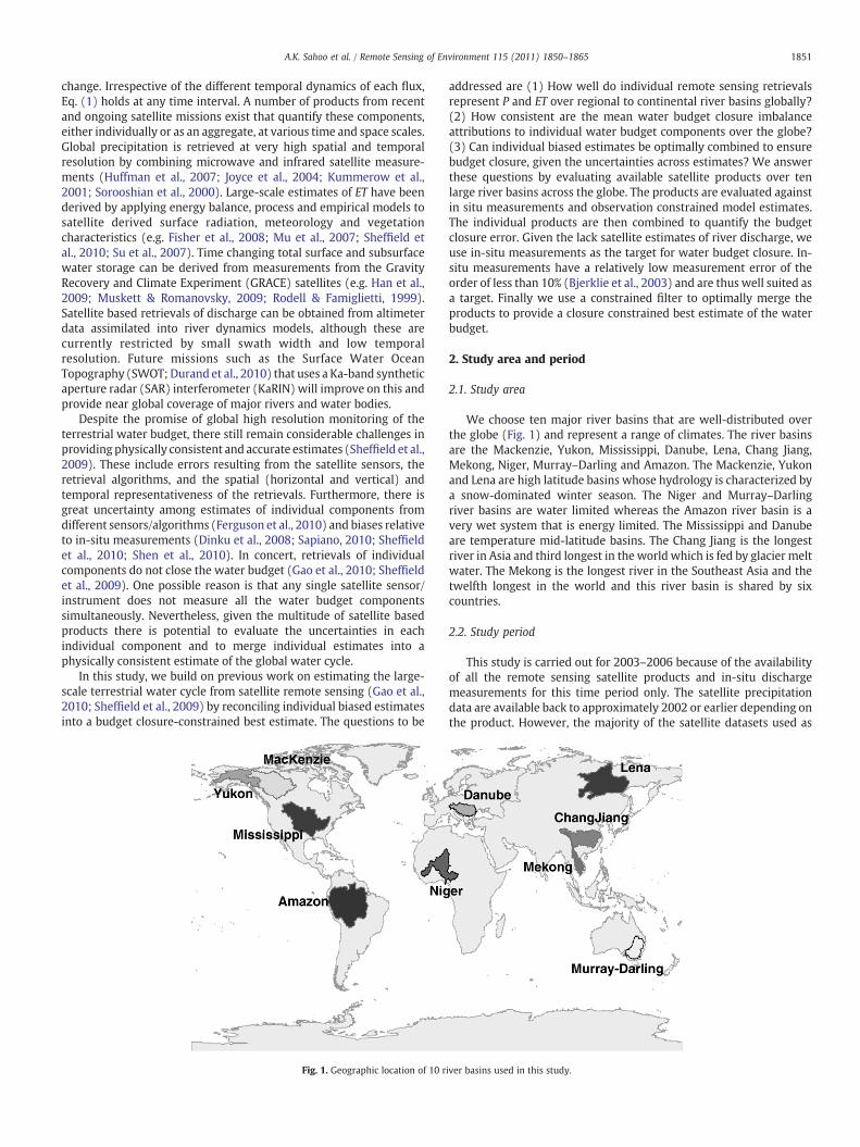
We choose ten major river basins that are well-distributed overthe globe (Fig. 1) and represent a range of climates. The river basinsare the Mackenzie, Yukon, Mississippi, Danube, Lena, Chang Jiang,Mekong, Niger, Murray–Darling and Amazon. The Mackenzie, Yukonand Lena are high latitude basins whose hydrology is characterized bya snow-dominated winter season. The Niger and Murray–Darlingriver basins are water limited whereas the Amazon river basin is avery wet system that is energy limited. The Mississippi and Danubeare temperature mid-latitude basins. The Chang Jiang is the longestriver in Asia and third longest in the world which is fed by glacier meltwater. The Mekong is the longest river in the Southeast Asia and thetwelfth longest in the world and this river basin is shared by sixcountries.

2.2. Study period

This study is carried out for 2003–2006 because of the availabilityof all the remote sensing satellite products and in-situ dischargemeasurements for this time period only. The satellite precipitationdata are available back to approximately 2002 or earlier depending onthe product. However, the majority of the satellite datasets used as

iver basins used in this study.

PRS1, PRS2, …

ETRS1, ETRS2, …

Pin-situ1, Pin-situ2, …

ETmodel1, ETmodel2, …

1852 A.K. Sahoo et al. / Remote Sensing of Environment 115 (2011) 1850–1865

input to the evapo-transpiration products is taken from the NationalAeronautics and Space Administration (NASA) Aqua satellite, whichhas been flying since 2002. Terrestrial water storage data are takenfrom the GRACE satellite (for details, see Appendix A), which are onlyavailable since 2003.

Merging

P’RS, ET’RS QOBS, dS/dtRS

Water Balance Constraint

P”, ET”, Q”, dS”/dt

Fig. 2. A flow-chart of the methodology used in this study.

3. Data and methodology

3.1. Datasets

Multiple satellite remote sensing datasets from various sources areused for each water cycle variable except water storage, which is onlyavailable from GRACE. Non-satellite data products that are based onin-situmeasurements, off-linemodeling or inferred from atmosphericreanalyses are used to estimate uncertainties in the satellite dataproducts. These multiple non-satellite products are merged togetherby taking their mean for each water budget components and the non-satellite merged products are assumed to represent our best estimatesof each budget term. The uncertainties are then used in the waterbudget analysis and to merge the satellite datasets to form a bestestimate of budget terms under a closure constraint. The datasets arelisted in Table 1 with a brief summary below. Details of all the satelliteand non-satellite products for each water budget component aregiven in the Appendix A.

Eight precipitation data products (four satellite and four non-satellite based) are considered. The satellite products are GPCP,TRMM, CMORPH and PERSIANN and the non-satellite products areCPC, CRU, WM and GPCC. Six ET data products are used of which fourare satellite-derived products and two are non-satellite products. Thesatellite products are PM (ISCCP), PM (EOS), PT (EOS), and SEBS (EOS)and the non-satellite products are VIC and ERA-interim inferred. Thesatellite data products are generated by forcing the PM, PT and SEBSmodels with input satellite data. The acronyms in parentheses aftereach ETmodel indicates the input data source used to generate the ETproduct. Discharge data are taken from in-situ gauge observationsfrom the Global Runoff Data Center (GRDC, 2010). Terrestrial waterstorage data are taken from the GRACE satellite products.

Even though Eq. (1) holds at any time scale, the GRACE storagedata are available at approximately monthly time scale and can onlybe considered for large river basins because of its coarse spatialresolution. Moreover, the in-situ discharge data are available at basinscale. Therefore, our study is focused on large river basins withmonthly time scale due to the lack of availability of the high resolutiondata products for all components. All the data products are temporallyand spatially averaged to monthly and river basin scale respectively.

Table 1Summary of the gridded datasets used in this study. Our study period is from 2003 to 2006

Dataset Start year End year Spatial resolu

GPCP 1997 2006 1°TMPA 3B42RT 1997 Present 0.25°CMORPH 2003 2006 8 km (at equaPERSIANN 2000 2006 0.25°CPC PREC\L 1950 Present 2.5°CRU TS3.0 1901 2006 0.5°WM v2.01 1900 2008 0.5°GPCC 1900 2007 0.5°PM (ISCCP) 1984 2005 2.5°PM (EOS) 2003 2006 5 kmPT (EOS) 2003 2006 5 kmSEBS (EOS) 2003 2006 5 kmVIC 1948 2006 1.0°ERA-interim 1989 2006 T255GRACE 2002 2006 Basin (750 kmGRDC ~1900 ~2006 Basin

3.2. Methods

Fig. 2 shows a basic flowchart of the analysis. First, the individualsatellite data products for P and ET are analyzed, and the uncertaintiesare calculated with respect to the non-satellite merged product (asexplained in Section 3.1) for each river basin separately. All thesatellite products (PRS1, PRS2 … and ETRS1, ETRS2 …) are then mergedtogether to produce a single satellite-only data product for P and ET(P′RS and ET′RS) respectively. Q and dS/dt for each river basin are takendirectly from the in-situmeasurements (QOBS) and the GRACE satellite(dS/dtRS) respectively for the water budget calculation. There areuncertainties in the river discharge in-situ measurement data becauseof a number of sources of errors, such as the water level measure-ments, the rating curves and changes in the channel morphology,which will vary from basin to basin. Without detailed errorinformation for each gauge, we assume that these in-situ dischargemeasurements are without any bias and they contain 7% RMS error(Dingman, 2002). The terrestrial storage data from GRACE mightcontain some bias, which depends on the basin and spatial domain,but there is no other large-scale estimate available to evaluate this.Land surface modeling can be used to evaluate GRACE (e.g. Tang et al.,2010), although these models generally do not account for all storagecomponents, such as groundwater. Hence, we consider GRACE to beun-biased and use the standard GRACE error value (Rodell et al., 2004;

. Some datasets may extend beyond our study period.

tion Temporal resolution Reference

Daily Adler et al. (2003)3 h Huffman et al. (2007)

tor) 30 min Joyce et al. (2004)3 h Hong et al. (2004)Monthly Chen et al. (2002)Monthly Mitchell and Jones (2005)Monthly Willmott and Matsuura (2010)Monthly Schneider et al. (2008)3 h Sheffield et al. (2010)Daily Vinukollu et al. (2011)Daily Vinukollu et al. (2011)Daily Vinukollu et al. (2011)3 h Sheffield and Wood (2007)12 h Simmons et al. (2007)

) ~Monthly Swenson and Wahr (2006)Monthly GRDC (2010)

1853A.K. Sahoo et al. / Remote Sensing of Environment 115 (2011) 1850–1865

Sheffield et al., 2009). All the estimates for P, ET, Q and dS/dt are thenpassed through a water budget closure constraint algorithm wherethe closure constraint is introduced as an error free observation (Pan &Wood, 2006).

3.2.1. Merging techniqueThe different satellite estimates of P and ET are merged into single

P and ET estimates. The merged estimate is a weighted average of allthe satellite products and the weights are determined by their errorlevels. First, the error variance of each product is calculated using themean of non-satellite estimates as the truth. The weights aredetermined by two conditions: (a) the weights sum up to 1; and(b) the weights are proportional to the inverse of the error variances.The weights are calculated as:

wi =1σ2i= ∑

n

j=1

1σ2j

ð2Þ

where, wi is the weight for product i, σi2 is the error variance of

product i, and n is the total number of products to merge. Thisweighting procedure ensures that the merged estimates have theminimal error variance (Luo et al., 2007).

3.2.2. Enforcing water balance constraintThe mass balance of water given by Eq. (1) indicates that there is

closure among the components. However, it is well known thatestimates of the water budget terms from individual sources do notpreserve this balance when combined and result in a residual orimbalance term (e.g. Pan & Wood, 2006). The Constrained EnsembleKalman Filter (CEnKF) has been proposed by Pan andWood (2006) toimpose a linear constraint on the estimates of water balance terms soas to force closure. CEnKF has a convenient two-step design where thefirst step is applied as a regular Ensemble Kalman Filter (EnKF) and

Fig. 3. Mean seasonal cycle of various precipitation products over 10 river basins for the perimerged product is shown in a solid line. The non-satellite merged product is a combination

the second step (constraining step) is performed separately to makefurther state updates such that the water balance is closed. Essentially,the constraining works by distributing the imbalance back to all waterbudget terms according to their error levels and correlations. Waterbudget terms with larger errors are adjusted more, i.e. more of theimbalance is attributed to them, and vice versa. The CEnKF constrain-ing procedure also works in non-ensemble form (Simon & Chia,2002), andwe apply this procedure after wemerge satellite estimates.The final results presented here perfectly close the water balancegiven by Eq. (1). This provides an improvement over the uncon-strained and merged estimates since it imposes a known physicalconstraint (mass balance) on the data, which cannot be applied to anyproduct individually.

4. Results and discussion

4.1. Estimation of uncertainties in the original RS data

We first assess each of the satellite P and ET products against thenon-satellite merged products over the ten basins. Fig. 3 shows themean seasonal cycle of the precipitation products calculated for 2003to 2006. The non-satellite merged dataset is the average of the gauge-based CPC, CRU, WM and GPCC products. There is no spatial coveragefor most satellite products at latitudes higher than ±50°, thereforeonly the GPCP satellite product is shown over the Mackenzie, Yukonand Lena river basins. A distinct seasonal cycle (higher precipitation insummer and lower in winter) is shown by all satellite and non-satellite merged products for all basins except the Murray–Darling.The summer precipitation is much higher over low-latitude basins(Niger, Amazon, andMekong; notice that the scale on the vertical axisis not same for all the basins). The satellite estimates differsignificantly for individual river basins though the phase of theseasonal cycles agrees well. For example, the difference between

od 2003 to 2006. The satellite products are shown in dashed lines and the non-satelliteof all the non-satellite based products: CPC, CRU, WM and GPCC.

1854 A.K. Sahoo et al. / Remote Sensing of Environment 115 (2011) 1850–1865

TRMM and PERSIANN mean precipitation is more than 70 mm inAugust over the Niger basin and the difference between the CMORPHand TRMM mean precipitation is more than 60 mm in February overthe Danube basin. There is no consistency in the relative order of thesatellite estimates datasets across the basins; e. g. TRMM estimatesthe highest P over the Danube whereas the GPCP estimates thehighest P over theMekong and PERSIANN estimates the highest P overthe Niger. All the satellite products overestimate precipitation ascompared to the non-satellitemergedproduct. Themonthlymeanbias(mmmonth−1) ranges between 33 (Mississippi) and −4 (Murray–Darling) for TRMM; 33 (Niger) and −7 (Mekong) for CMOPRH; 45(Niger) and −13 (Danube) for PERSIANN; and 19 (Yukon) and −8(Amazon) for GPCP. Similarly, the RMSE (mmmonth−1) rangesbetween 43 (Mississippi) and 17 (Murray–Darling) for TRMM; 46(Niger) and 20 (Chang Jiang) for CMOPRH; 61 (Niger) and 19(Murray–Darling) for PERSIANN; and 29 (Mekong) and 9 (Lena) forGPCP (see Table 2 for the complete list of bias and RMSE values).Among all the satellite precipitation estimates, theGPCP seasonal cyclefollows most closely with the non-satellite merged dataset and it hascomparatively lower bias and RMSE values (note that the GPCPdatasetused here is the non-gauge corrected, satellite only version).

Fig. 4 shows the mean seasonal cycle of the ET products calculatedfor 2003 to 2006. The seasonal cycles for the low-latitude basins(Mekong, Amazon and Murray–Darling) are not as prominent as inthe high latitude basins. The phase of the seasonal cycle is mostlyconsistent among the products except over the Amazon. The SEBS(EOS) ET product is always higher in the summer months over allbasins. The SEBS (EOS) also gives negative ET during the wintermonths over the high latitude basins whereas the other satelliteproducts estimate nearly zero, but positive, values. Therefore thedifference in ET between the summer and winter peaks for the SEBS(EOS) is large over the high latitude basins. The monthly mean bias(mmmonth−1) ranges between 21 (Mekong) and−11 (Danube) forPM(ISCCP); 13 (Yukon) and −30 (Mississippi) for PM (EOS); 22(Murray–Darling) and−17 (Mississippi) for PT (EOS); and 53 (ChangJiang) and 4 (Mackenzie) for SEBS (EOS). Similarly, the RMSE(mmmonth−1) ranges between 33 (Amazon) and 6 (Mackenzie)for PM (ISCCP); 37 (Mississippi) and 8 (Lena) for PM (EOS); 34(Mekong) and 7 (Lena) for PT (EOS); and 60 (Chang Jiang) and 25(Danube) for SEBS (EOS) in mmmonth−1 (see Table 3 for thecomplete list of bias and RMSE values). The large differences betweenthe ET products are mainly due to the different sensitivities of eachmodel to forcing uncertainty (Vinukollu & Wood, in preparation). Forexample, the SEBS model is sensitive to inconsistencies in the air andsurface temperature inputs, whereas these are relatively unimportantfor the PM model.

In terms of partitioning of P into ET and Q, a significant portion ofthe precipitation water is partitioned to Q over low-latitude basins(Amazon, Chang Jiang and Mekong) whereas a significant portion of Pis partitioned to ET over the other basins.

Table 2Bias and RMSE values of different satellite precipitation (P) products with respect to the no

Bias

TRMM CMORPH PERSIANN G

Mackenzie – – –

Yukon – – –

Mississippi 33.33 20.58 26.86Danube 18.95 −13.48 −12.72Lena – – –

Chang Jiang 0.87 −6.26 −10.95 −Mekong −4.35 −6.57 −7.79Niger 20.37 33.18 45Murray–Darling −4.48 2.63 −4.26Amazon 6.83 24.99 8.91 −

4.2. Merging of the satellite P and ET products

The satellite estimates for P and ET show little agreement acrossthe basins, although there is some consistency in the phase of theirseasonal cycles. Hence we merge all the satellite products based ontheir relative uncertainties before estimating water budget. Forbrevity, we discuss the results in detail only for the Amazon andMississippi, and provide a summary for the other basins. Figs. 5 and 6show the merging results for P (left panel) and ET (right panel) overthe Mississippi (Fig. 5) and Amazon (Fig. 6) river basins. For theMississippi (Fig. 5, left panel), the GPCP precipitation is much lowerthan the other satellite products and is very consistent with the non-satellite merged P time series over the whole time period. The TRMMestimate exhibits opposite phase during the winter of 2003–2004. Allthe original satellite products estimate low P in the summer of 2006and the biases for all the satellite products with respect to the non-satellite merged product are also small during that time period. Theseasonality is clearly evident in all the datasets. All the original ETproducts show a reasonable seasonality over the Mississippi riverbasin (Fig. 5, right panel) which corresponds to the seasonality seen inthe P products. The SEBS (EOS) shows a smaller second peak for ET inthe spring season as well. However, the ET estimates differ from eachother by considerably large values relative to the differences for P. PM(EOS) has the lowest mean ET (b50 mm month−1) whereas the SEBS(EOS) has the highest ET (N100 mmmonth−1; note that the scale hasbeen truncated for clarity). The maximum difference between thesetwo products approaches 110 mmmonth−1 in the summer. The PM(ISCCP) and PT (EOS) have intermediate ET values. Overall, the PM(ISCCP) ET product is the closest to the non-satellite merged ETdataset.

For the Amazon (Fig. 6, left panel), all the satellite P products showreasonable seasonal cycles (higher in summer and lower in winter)compared to the non-satellite merged dataset, although the summerpeak for the satellite products (except GPCP) is about 1–2 monthsearlier. The P seasonal range is very similar across all products exceptin the summer season of 2004, when the PERSIANN and CMORPHproducts are high. The ET products over the Amazon are very differentfrom each other (Fig. 6, right panel), in terms of the mean andseasonal cycle. The PM (ISCCP) and SEBS (EOS) ET estimates are muchhigher than the other products and the difference for these twoestimates with respect to the other estimates range in the order of 30to 50 mmmonth−1 in winter seasons. These two products show sameseasonality and the estimates are similar to each other. The PT (EOS)product has the lowest ET values. It shows a marked seasonal cycle,but in opposite phase to the PM (ISCCP) and SEBS (EOS). The non-satellite merged product and the PM (EOS) do not show anyseasonality but do show a positive trend, which is larger for the PM(EOS) product.

For the merged P and ET datasets (Figs. 5 and 6, bottom row), weuse four satellite based P and ET products respectively. The shaded

n-satellite merged product over ten river basins.

RMSE

PCP TRMM CMORPH PERSIANN GPCP

6.97 – – – 9.6919.4 – – – 23.9610.69 43.35 40.22 39.24 16.6113.83 32.86 29.26 36.97 21.215.22 – – – 8.931.32 22.52 19.67 29.42 17.299.22 42.19 34.10 38.66 28.535.64 29.04 45.85 60.70 11.061.97 17.15 22.21 18.52 13.967.90 43.04 54.42 52.82 18

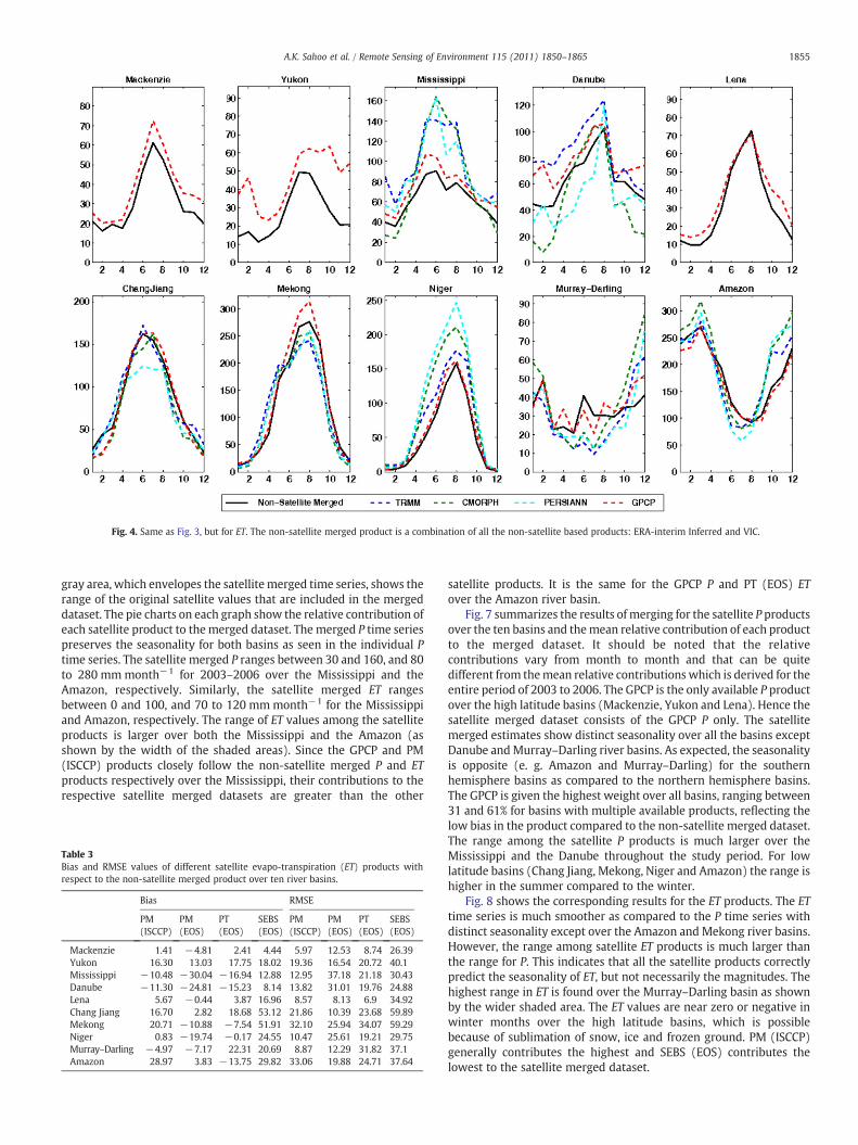
Fig. 4. Same as Fig. 3, but for ET. The non-satellite merged product is a combination of all the non-satellite based products: ERA-interim Inferred and VIC.

1855A.K. Sahoo et al. / Remote Sensing of Environment 115 (2011) 1850–1865

gray area, which envelopes the satellite merged time series, shows therange of the original satellite values that are included in the mergeddataset. The pie charts on each graph show the relative contribution ofeach satellite product to themerged dataset. The merged P time seriespreserves the seasonality for both basins as seen in the individual Ptime series. The satellite merged P ranges between 30 and 160, and 80to 280 mmmonth−1 for 2003–2006 over the Mississippi and theAmazon, respectively. Similarly, the satellite merged ET rangesbetween 0 and 100, and 70 to 120 mmmonth−1 for the Mississippiand Amazon, respectively. The range of ET values among the satelliteproducts is larger over both the Mississippi and the Amazon (asshown by the width of the shaded areas). Since the GPCP and PM(ISCCP) products closely follow the non-satellite merged P and ETproducts respectively over the Mississippi, their contributions to therespective satellite merged datasets are greater than the other

Table 3Bias and RMSE values of different satellite evapo-transpiration (ET) products withrespect to the non-satellite merged product over ten river basins.

Bias RMSE

PM(ISCCP)

PM(EOS)

PT(EOS)

SEBS(EOS)

PM(ISCCP)

PM(EOS)

PT(EOS)

SEBS(EOS)

Mackenzie 1.41 −4.81 2.41 4.44 5.97 12.53 8.74 26.39Yukon 16.30 13.03 17.75 18.02 19.36 16.54 20.72 40.1Mississippi −10.48 −30.04 −16.94 12.88 12.95 37.18 21.18 30.43Danube −11.30 −24.81 −15.23 8.14 13.82 31.01 19.76 24.88Lena 5.67 −0.44 3.87 16.96 8.57 8.13 6.9 34.92Chang Jiang 16.70 2.82 18.68 53.12 21.86 10.39 23.68 59.89Mekong 20.71 −10.88 −7.54 51.91 32.10 25.94 34.07 59.29Niger 0.83 −19.74 −0.17 24.55 10.47 25.61 19.21 29.75Murray–Darling −4.97 −7.17 22.31 20.69 8.87 12.29 31.82 37.1Amazon 28.97 3.83 −13.75 29.82 33.06 19.88 24.71 37.64

satellite products. It is the same for the GPCP P and PT (EOS) ETover the Amazon river basin.

Fig. 7 summarizes the results of merging for the satellite P productsover the ten basins and themean relative contribution of each productto the merged dataset. It should be noted that the relativecontributions vary from month to month and that can be quitedifferent from themean relative contributions which is derived for theentire period of 2003 to 2006. The GPCP is the only available P productover the high latitude basins (Mackenzie, Yukon and Lena). Hence thesatellite merged dataset consists of the GPCP P only. The satellitemerged estimates show distinct seasonality over all the basins exceptDanube andMurray–Darling river basins. As expected, the seasonalityis opposite (e. g. Amazon and Murray–Darling) for the southernhemisphere basins as compared to the northern hemisphere basins.The GPCP is given the highest weight over all basins, ranging between31 and 61% for basins with multiple available products, reflecting thelow bias in the product compared to the non-satellite merged dataset.The range among the satellite P products is much larger over theMississippi and the Danube throughout the study period. For lowlatitude basins (Chang Jiang, Mekong, Niger and Amazon) the range ishigher in the summer compared to the winter.

Fig. 8 shows the corresponding results for the ET products. The ETtime series is much smoother as compared to the P time series withdistinct seasonality except over the Amazon and Mekong river basins.However, the range among satellite ET products is much larger thanthe range for P. This indicates that all the satellite products correctlypredict the seasonality of ET, but not necessarily the magnitudes. Thehighest range in ET is found over the Murray–Darling basin as shownby the wider shaded area. The ET values are near zero or negative inwinter months over the high latitude basins, which is possiblebecause of sublimation of snow, ice and frozen ground. PM (ISCCP)generally contributes the highest and SEBS (EOS) contributes thelowest to the satellite merged dataset.

Fig. 5. Results of precipitation (left panel) and evapo-transpiration (right panel) merging over the Mississippi river basin. The top row shows the original time series and the bottomrow shows the merged time series of the original satellite data for P and ET for the period 2003 to 2006. The shaded area in the bottom figures shows the range of the values fromvarious satellite products used in the satellite merged product. The inserted pie chart indicated the relative contributions of each P and ET component in the merged product.

1856 A.K. Sahoo et al. / Remote Sensing of Environment 115 (2011) 1850–1865

4.3. Water balance closure

Figs. 9 and 10 show the results for the water budget componentsand budget closure from the satellite only products for 2003–2006 forthe unconstrained (left panel) and constrained system (right panel).The respective satellite products are merged together for each waterbudget component and these merged satellite only water budgetcomponents are used to estimate the water budget closure. In theunconstrained system, the water budget calculated using data fromvarious satellites will generally not close because of errors inindividual products. In the constrained system, we force the closureof the water budget. The results are again shown for the MississippiRiver (Fig. 9) and Amazon (Fig. 10) River basins. The top row showsthe fluxes, the middle row shows the terrestrial water storage and thebottom row shows the imbalance after calculating the water budget(Eq. 1). The river discharge data are taken from the in-situ gaugeobservations, which represent the entire basin. The storage iscalculated from the GRACE satellite product and then the standard

Fig. 6. Same as Fig. 5, but for

error value is added to it. There is no bias correction applied to thedischarge and storage terms. Over the Mississippi basin, Q is relativelysmall compared to ET, and P is generally higher than ET+Q, whichimplies an increase in storage or water balance error. dS/dt showsseasonality over the Mississippi basin with positive storage change inwinter and negative change in summer. The change in storage valuesvary between −60 and 30 mmmonth−1. When the unconstrainedwater budget is calculated, it is found that it does not close overthe Mississippi. The imbalance varies between about 0 and 70 mmmonth−1 and shows a seasonal cycle. The positive imbalance derivesmostly from the higher P values relative to the other components.These imbalance values are distributed among each water budgetcomponent using the CEnKF method as described in Section 3.2.2 togive a constrained water budget (Fig. 9, right panel). The readjustedfluxes and storage change values maintain similar seasonal cycles tothe unconstrained water budget components but the magnitudes areshifted, indicating that our approach of constraining the water budgetcomponents does not alter their behavior. The water budget closure

the Amazon river basin.

Fig. 7. Summary of the results of the merging of satellite P products over all the 10 basins and their mean relative contributions (inserted pie charts) to the merged product. Theshaded area in the bottom figures shows the range of the values from various satellite products used in the satellite merged product.

1857A.K. Sahoo et al. / Remote Sensing of Environment 115 (2011) 1850–1865

results are shown in the bottom right panel of Fig. 9, and showsperfect closure of the water budget. The pie chart reveals the relativeattribution of the non-closure error to each water budget component(a higher value indicates a higher contribution of that component tothe non-closure error). The majority of the non-closure error isattributable to the P estimate and this is also shown in the adjustedvalues for P in the upper right panel of Fig. 9 for which the constraint isapplied (compare the two P time series in the top row).

Fig. 10 shows the results for the Amazon. Again, notice the lack ofseasonal cycle in the ET dataset in both the non-constrained andconstrained system. The imbalance in the water budget closure ismuch larger than for the Mississippi (varying between −70 and50 mmmonth−1). The storage change and water budget closureimbalance show seasonality over this basin. Most of the non-closureerror is assigned to the P and ET components. Table 4 summarizes thenon-closure for all basins, in terms of the seasonal range in the error.

Fig. 11 summarizes the mean water budget non-closure error(imbalance) attribution for all ten basins. The percent values shown ineach pie chart are calculated based on the absolute imbalance values

and they are not normalized by the respective water budgetcomponent values. Very little imbalance is attributed to Q becausethe in-situ gauge measurements are assumed to have less uncertaintythan the satellite products. In contrast, a major portion of theimbalance is attributed to P over all basins, which is up to 55% for theYukon basin. This is because precipitation is the largest component ofthe water budget and the uncertainties across satellite products arehigher than for other components. The bias correction impacts themagnitude of each water budget component significantly though itclosely follows the partitioning ratio of P into ET and Q as we notice inthe non-bias corrected case.

4.4. Impact of bias correction on satellite based estimates

The seasonal biases for different satellite estimates with respect tothe non-satellite merged estimate range very widely for both P and ETas we notice from Figs. 2 and 3 respectively. An obvious questionarises: do we need to bias correct the individual satellite productsbefore merging them together to estimate the water budget? In

Fig. 8. Same as Fig. 7, but for ET.

1858 A.K. Sahoo et al. / Remote Sensing of Environment 115 (2011) 1850–1865

another words, what is the impact of the bias correction on the waterbudget estimated from the satellite products? This section looks at theabove question by comparing the original and bias corrected satellitederived results. The satellite products are bias corrected to the non-satellite merged products for this study. It is reminded that the non-satellite merged products are based on in-situ measurements for P,and estimates from land surface model simulations and inferred fromatmospheric reanalysis for ET. Figs. 12 and 13 compare the waterbudget imbalance and components calculated from the original (toprow) and bias corrected satellite products (bottom row) for theMississippi (Fig. 12) and Amazon (Fig. 13). The imbalance calculatedfrom the original satellite data is much higher throughout the studyperiod and sometimes exceeds 50 mmmonth−1 for the Mississippi.In contrast, the imbalance is much lower for the bias correctedsatellite products. This indicates that bias correction of the originalsatellite products helps to remove the higher imbalance values overtheMississippi. However, when the water budget closure constraint isapplied in both the cases (removing the imbalance) and the non-closure error is assigned to the water budget components, thereadjusted results for the water budget components exhibit similar

temporal variation and the values are not significantly differentbetween the two cases. Over the Amazon (Fig. 13), the imbalancecalculated from both the original and bias corrected satellite datasetsare very similar to each other. This implies that the bias correction tothe satellite products with respect to the non-satellite mergedproduct is unable to remove the higher imbalance over this basin.As expected, the corrected water budget components after the waterbudget closure is very similar in both cases.

It is evident that the bias corrected results are largely influenced bythe quality of the non-satellitemerged products. Inwell-instrumentedregions like the Mississippi, the non-satellite merged products arerelatively accurate, whereas their accuracy in the Amazon is relativelylow due to the sparsity of gauges and unique riverine system. This islikely the case for many other parts of the world, especially in under-developed countries.

On the other hand, the water balance closure constraint applied inthis study may not quantify the water budget components correctly ifa bias is present in those components prior to applying the waterbudget closure constraint. For example, if both P and ET are positivelyand equally biased, these biases would cancel each other in the water

Fig. 9. The results for the water budget closure from the satellite only products for 2003 to 2006 period using the unconstrained (left panel) and constrained system (right panel) forthe Mississippi river basin. The top row shows the fluxes, middle row shows the terrestrial water storage and the bottom row shows the imbalance after water budget estimation.The inserted pie chart shows the relative assignment of the non-closure error to various water budget components based on their relative uncertainties.

1859A.K. Sahoo et al. / Remote Sensing of Environment 115 (2011) 1850–1865

budget to produce zero closure imbalances. In this case, the waterbudget constraint algorithm assumes that both the P and ET estimatesare accurate and will not correct them, resulting in overestimates ofthese components.

It is therefore an open question as to whether we need to biascorrect the satellite products prior to applying the water budget

Fig. 10. Same as Fig. 9, but for

closure constraint; knowing that the non-satellite merged productsmay have large uncertainties themselves and may do little to biascorrect the satellite products and the water budget closure constraintmight not quantify the uncertainties properly in the satellite productsdue to the bias. Nevertheless, we use the original satellite products forthe water budget closure in this study, because (i) the variability and

the Amazon river basin.

Table 4Range of water budget non-closure errors at all the ten river basins.

Range of WB non-closure error(mm month−1)

Mackenzie −18 to 32Yukon −57 to 55Mississippi 0 to 70Danube −20 to 42Lena −60 to 47Chang Jiang −35 to 50Mekong −32 to 73Niger −5 to 49Murray–Darling −32 to 43Amazon −70 to 50

1860 A.K. Sahoo et al. / Remote Sensing of Environment 115 (2011) 1850–1865

mean of the adjusted water budget components after applying thewater budget closure constraint is very similar when using either theoriginal or bias corrected satellite products and (ii) we assume thatthe uncertainties present in the adjusted water budget components,after imposing the water budget closure, are less than those of thenon-satellite merged products that are used to do the bias correction.

5. Conclusion

The goal of this study is to estimate the water budget from satellitederived products over ten river basins for the period 2003–2006. Wehave considered multiple remote sensing estimates of precipitation,evapo-transpiration and change in storage. A non-satellite (including

Fig. 11. The summary diagram of mean imbalance attribution charts over all the 10 river bimbalance values and are not normalized by the respective water budget component value

in-situ observations, land surface model data, and reanalysis data)merged (assuming zero bias in the non-satellite datasets) product,developed separately for P and ET, has been used as a target dataset tocalculate the uncertainties in the satellite products. The seasonal cyclesformost of the satellite P and ET products are generally consistentwitheach other andwith the non-satellitemerged products. This consistentpattern among the different products is attributed to the similar set ofsatellite instruments that most algorithms use to estimate the watercycle components. However, there are huge discrepancies in theabsolute values among the products, which can be partly attributed tothe different retrieval algorithms. All the satellite products tend tooverestimate precipitation for most of the basins, especially in thesummer. TheGPCP P and PM(ISCCP) ETproducts are found to have lessbias and uncertainties over most of the basins.

When the water budget is calculated from the satellite products,there is non-zero closure, which is consistent with the findings fromearlier satellite based water budget studies (Gao et al., 2010; Sheffieldet al., 2009). This non-closure is attributable to a number of factors.The spatial and temporal resolution at which each water budgetvariable is generated can affect the errors in the individual variables(e.g. Kustas et al., 2004; McCabe &Wood, 2006) as well as mismatchesbetween variables (e.g. the GRACE storage change term has thecoarsest spatial and temporal resolution whereas the ET retrievals aregenerallymade at 5–10 km and sub-daily resolution). The GRACE datamay also suffer from the leakage of the signal from outside of the basinboundary (Swenson & Wahr, 2006), which will vary from basin tobasin depending on size and shape. The dynamic range and

asins. The percent values shown in each pie chart are calculated based on the absolutes. See Fig. 1 for the name of the basins.

Fig. 12. Comparison of the water budget imbalance and components calculated from the original (top row) and bias corrected satellite products (bottom row) for the Mississippiriver basin. The left panel shows the imbalances and the right panel shows the adjusted water budget components after the water budget closure is applied.

1861A.K. Sahoo et al. / Remote Sensing of Environment 115 (2011) 1850–1865

uncertainties associated with each retrieval algorithm for eachvariable can also influence the non-closure. For example, precipitationretrievals from different algorithms show large discrepancies,especially over complex terrain (e.g. Dinku et al., 2008) andfor non-convective, wintertime precipitation (Ebert et al., 2007;Gottschalck et al., 2005; Tian et al., 2007). Finally, the differences ininput data from different sensors or providers can have large impactson the retrievals, for example on ET (Ferguson et al., 2010).

The magnitude of the non-closure error varies from basin to basin(Table 4). It is greatest over the Amazon and lowest over theMackenzie,Niger and Danube basins. This may be a reflection of the sparseness ofin-situmeasurements in the Amazon towhich satellite estimates can becalibrated to. In fact, for the Amazon there are large uncertainties inwater budget components from ground-based measurements (Costa &Foley, 1998; Fekete et al., 2004), and disagreement between observa-tions,models and reanalyses in precipitation (Adler et al., 2001) and themagnitude of the seasonal cycle of ET (Jimenez et al., 2011). However,there is considerable variation in non-closure errors across the otherbasinswith lowerror values for theNiger, for example,which is also lesswell monitored. In high latitudes where observations are also generallysparse and the water budget is complicated by cold season processes,the non-closure error is high for two basins (Lena and Yukon) but theleast of all basins for the Mackenzie. Thus there appears to be noconsistent relationship between budget closure error and observationaldensity, climate, or even basin size.

Fig. 13. Same as Fig. 12, but fo

Irrespective of all the inconsistencies among the various dataproducts, we enforce a water budget constraint scheme to close thewater budget as derived from the satellite products and calculate therelative contribution of each water budget component to the closureimbalance error. Our approach ensures the closure of the waterbudget in this study. The precipitation products provide the largestsource of the non-closure error, suggesting that the satelliteprecipitation has the largest uncertainties among the three satellitemerged products. The attribution of most of the non-closure error tothe precipitation component is very consistent across all the basins.This is a reflection of the spatial and temporal variability ofprecipitation and the difficulty in obtaining accurate retrievals fromsatellite measurements that have low temporal repeat sampling (e.g.Hossain & Anagnostou, 2004; Nijssen & Lettenmaier, 2004; Steiner etal., 2003) and are reliant on conversion of radiances to rain rates(McCollum et al., 2002). Discharge tends to have the lowestcontribution to non-closure error, which is generally because of therelatively low uncertainties that are assigned based on literaturevalues. The contribution of dS/dt is comparable to that of P, and evenlarger in the Lena basin, where the seasonal cycle of discharge isdominated by the spring snow melt (Troy & Wood, 2010), implyingthat uncertainties in the change in storage are important.

There is a wide range of biases across the satellite estimates withrespect to the non-satellite merged estimate. Therefore, we verifiedthe impact of bias correction on our water budget calculation error.

r the Amazon river basin.

1862 A.K. Sahoo et al. / Remote Sensing of Environment 115 (2011) 1850–1865

The results indicate that the impact of bias correction depends on howskillful and accurate our target non-satellite merged estimate is overany river basin. Many continental river basins (especially in the leastdeveloped regions such as in Africa) do not have extensive in-situobservation networks and therefore, the non-satellite mergedestimate over those basins might carry larger uncertainties, asdiscussed above for the Amazon. Thus, the bias correction to thesatellite estimates based on the non-satellite merged product may nothave any impact over those basins.

The biases and random errors in the satellite estimates can bereduced through calibration, which will lead to a reduction in thebudget closure error. For precipitation, satellite estimates can becalibrated to gauge measurements and this has been done for thealgorithm calibration for the real-time version of the TRMM estimatesin 2008. For ET, this is more problematic because of the lack of large-scale measurements, although modeled and infrared data can be usedas a target for calibration in regions where there is confidence in theirestimates. However, our merging technique is robust and indepen-dent of whether the datasets are calibrated or not.

To conclude, this study provides initial estimates of the closedwater budget from satellite only products over ten continental riverbasins. We believe that these estimates from the merged satelliteproducts carry significant amounts of information about the watercycle in these basins and can be used as the basis for monitoring,climate change analysis and diagnostic studies. Further work isneeded to understand and attribute the source of the largediscrepancies among different estimates (satellite, in-situ, modeland reanalyses) of the water budget components in order to improvewater budget closure further at basin to continental scales andidentify where improvements to satellite retrieval systems are mostneeded.

Acknowledgements

This study is supported by National Aeronautics and SpaceAdministration under Grants NNX08AN40A and NNX09AK35G toPrinceton University. We thank the anonymous reviewer for theconstructive comments to improve this manuscript.

Appendix A. Datasets

Appendix A.1. Precipitation

Appendix A.1.1. GPCPThe Global Precipitation Climatology Project (GPCP) Version 2.1

precipitation product is a merged product that includes the low-orbitsatellite microwave, geostationary infrared and surface rain gaugeobservations of precipitation (Adler et al., 2003). The detailedmergingtechnique is described in Adler et al. (1993). The data are availablefrom 1979 to present, however the data prior to 1987 do not includeany microwave observations. This global monthly data product isprovided at 2.5°×2.5° spatial resolution. The product includes asatellite only dataset (without any gauge correction) as well, whichwe use in this study.

Appendix A.1.2. TMPA 3B42RTThe TRMM (Tropical Rainfall Measuring Mission) Multi Satellite

Precipitation Analysis (TMPA) precipitation product is based on acombination of the observations from the Low Earth Observing (LEO)microwave (MW) and Geosynchronous Earth Orbit (GEO) infrared(IR) satellite estimates (Huffman et al., 2007). The product is 3-hourly,0.25°×0.25° gridded dataset covering the region from 50°N to 50°Slatitude lines. The microwave data produce better estimates of theprecipitation due to their stronger relationship to precipitation, butthey are coarse in space and time whereas the infrared data producelower quality estimates, but at finer space–time scale. Hence, the

product first uses themicrowave datawherever they are available andthen fills in the areas with the IR datasets (Habib et al., 2009). TMPAproduces two datasets: one is bias corrected (3B42v6) and the other isin real time without any gauge correction (3B42RT). We use the3B42RT data product in this study.

Appendix A.1.3. CMORPHCPC (Climate Prediction Center) Morphing Technique (CMORPH)

products are derived using a morphing algorithm. First, this techniqueproduces propagation vector matrices by computing spatial lagcorrelations on successive geostationary satellite infrared imagesand uses these propagation vectors to propagate the microwavederived precipitation estimates (Joyce et al., 2004). This techniqueonly propagates the precipitation features, but performs time-weighting interpolation between the propagated features to deter-mine the shape and intensity of the precipitation feature. This is amerging technique and is very flexible in its nature. The CMORPHproducts are available from 60°N to 60°S at fine spatial (0.08°) andtemporal (30 min) resolutions.

Appendix A.1.4. PERSIANNPrecipitation Estimation from Remotely Sensed Information using

Artificial Neural Networks (PERSIANN) precipitation product isderived by merging various low altitude polar orbiting satellitesfrom NASA, NOAA and DMSP and Geostationary infrared imageryusing artificial neural network approach (Hsu et al., 1999; Sorooshianet al., 2000). The algorithm first extracts and classifies local texturefeatures from the infrared images to a number of texture patterns, andthen it associates those classified cloud texture patterns to the surfacerainfall rates. PERSIANN model parameters are then adjusted frompassivemicrowave rainfall estimates. PERSIANN precipitation productcovers from 50°N to 50°S at 0.25° spatial resolution and hourlytemporal resolution.

Appendix A.1.5. CPC unified gauge datasetThe CPC (Chen et al., 2002) precipitation dataset is created using a

reconstruction technique where the precipitation over land (PREC/L)is derived by interpolating observations from around 17,000 stationscollected in Global Historical Climatology Network (GHCN), and theClimate Anomaly Monitoring System (CAMS) datasets and theprecipitation over ocean (PREC/O) is derived by EOF reconstructionof historical observations. The optimal interpolation (OI) algorithm isused for the interpolation of the observations over the land. Themonthly data are available at 2.5°×2.5° spatial resolution from 1948to present.

Appendix A.1.6. CRUThe Climate Research Unit (CRU) of the University of East Anglia

(UK) produce a dataset of monthly surface-based climate parameters.Precipitation is one of the parameters included in that dataset which isgenerated from the available gauge datasets. The number of availableprecipitation gauges varies over the years: in 1901, 4957 gaugescontribute to the dataset, peaking in 1981 with 14,579 gauges. TheCRU inserts synthetic zero anomaly values in regions that are “too far”from observations (i.e. farther than 450 km), while the other schemessimply interpolate over the entire distance (New et al., 2000; Mitchell& Jones, 2005). The data are provided at 0.5° resolution globally.

Appendix A.1.7. WMCort Willmott and Kenji Matsuura (WM) of the University of

Delaware produce a climatic data product from a large number ofstations, both from the GHCN and from the archive of Legates andWillmott (1990). The data product includes monthly climatology anda monthly time series from 1900 to 2006 of the surface precipitationand air temperature. It is a land-only product. The data product isbeing improved continuously with better spatial interpolation

1863A.K. Sahoo et al. / Remote Sensing of Environment 115 (2011) 1850–1865

(gridding) algorithm and as more data becoming available from thestations (Willmott & Matsuura, 1995).

Appendix A.1.8. GPCCThe Global Climatology Precipitation Center (GPCC) provides three

monthly global precipitation data products based on the in-situ gaugeobservations. The GPCC Full Data product uses the near-real timegauge data collected from the World Meteorological Organization's(WMO) Global Telecommunication System and non-real time datasubmitted by almost 170 WMO member countries. The number ofavailable stations varies between 10,000 and 40,000 per month whocontribute data to the GPCC product. The Full Data product isoptimized for spatial density and accuracy. The data processingsteps include the quality control, quality assurance and interpolationto the desired grid size. The monthly data are provided globally at 1°spatial resolution (Rudolf & Schneider, 2005).

Appendix A.2. Evapo-transpiration (ET)

Appendix A.2.1. Penmen–Monteith (PM) modelA revised RS–PM formulation presented byMu et al. (2007) is used

in this study which is based on the Penman–Monteith equation(Monteith, 1965). This RS–PM method requires both an aerodynamicand canopy (or surface) resistances along with the available energy tocalculate the ET. A detailed description of the implementation of thisPMmethod can be found in Ferguson et al. (2010). The PM ET data arecollected from a global (only land) 5 km product for 2003 to 2006period.

Appendix A.2.2. Priestly–Taylor (PT) modelThe Priestly–Taylor (Priestley & Taylor, 1972) approach which was

initially developed to calculate ET over the well watered surface waslater modified to include the transpiration from the water stresssurface (Fisher et al., 2008). The PT method considers the effects oftemperature, vapor pressure deficit (VPD) and soil moisture to deriveconstraints representing canopy conductance. The PT data aregenerated at the same resolution as the PM data for 2003 to 2006period.

Appendix A.2.3. Surface energy balance system (SEBS)The surface energy balance system (SEBS) partitions the available

energy between the turbulent heat fluxes. The roughness parametersfor heat and momentum were estimated using the kB−1 (inverseStanton number) models as proposed byMassman (1999) and Blümel(1999). We take the mean of the roughness length estimates here,calculated by the above two methods. SEBS algorithm can be found inSu (2002). The SEBS data also are at 5 km resolution over the globalland regions from 2003 to 2006. For details about the ET datasets,please refer to Vinukollu et al. (2011).

Appendix A.2.4. Earth observing system (EOS) input datasetsIn this study, surface meteorological data, radiative energy flux

data and vegetation parameters are acquired from the AtmosphericInfrared Sounder (AIRS), the Clouds and the Earth's Radiant EnergySystem (CERES), and the Moderate Resolution Imaging Spectro-radiometer (MODIS) aboard the NASA Aqua-EOS platform for all thethree models. Instantaneous estimates of ET are calculated at thesatellite overpass time (1:30 pm local time) and then extrapolated todaily values assuming a constant daytime evaporative fraction (Crago& Brutsaert, 1996) and using hourly net radiation data from theSurface Radiation Budget (SRB; Stackhouse et al., 2000).

Appendix A.2.5. ISCCP input datasetsThe International Satellite Cloud Climatology Project (ISCCP)

(Schiffer & Rossow, 1983) was established in 1982 as a part of theWorld Climate Research Program (WCRP) to collect and analyze

operational geostationary and polar-orbiting meteorological satelliteradiance measurements to infer the global distribution of clouds andtheir role in radiation and the hydrologic cycle (Rossow & Duenas,2004). We use the Climatological Summary Product (FD-SRF) RadFluxversion of the dataset, which contains surface radiative fluxes and asummary of the physical quantities used to calculate them. Shortwaveand longwave radiative flux profiles are calculated using remotelysensed and modeled datasets to specify the properties of Earth'satmosphere and surface. We use the monthly averaged dataresampled at 2.5° equal angle resolution in this study.

Appendix A.2.6. VICThe Variable Infiltration Capacity (VIC) land surface model is a

large-scale hydrologic model that solves for both water and energybudget closure at the land surface (Liang et al., 1994, 1996). Therequired input atmospheric forcing variables to simulate VIC are takenfrom the Princeton Global Forcing (PGF) dataset (Sheffield et al.,2006) which usesmonthly observations to bias correct and downscalethe NCEP/NCAR reanalysis (Kalnay et al., 1996), resulting in a 3-hourlydataset from 1901 to 2006 at 1° resolution. The VIC model hasparticipated in many model inter-comparison studies and hasperformed reasonably well. It has been calibrated to measureddischarge at a number of unmanaged basins over USA (Troy et al.,2008) and Mexico (Zhu & Lettenmaier, 2007) and is expected toprovide reasonable estimates of ET.

Appendix A.2.7. ERA-interim inferredThe ERA-interim is a global reanalysis from ECMWF with data

available from 1989 through near real-time (Simmons et al., 2007).This reanalysis product does not close the water budget, and soilmoisture in this product is adjusted to match satellite brightnesstemperatures. The ET product used in this study has been inferredfrom the ERA interim product through equating the equations of massconservation for the atmosphere water budget. A detailed descriptionof thismethodology is provided in Troy et al. (2008).Wewill refer thisET product as ERA-interim inferred dataset hereafter.

Appendix A.3. Terrestrial water storage

Appendix A.3.1. GRACEThe Gravity Recovery and Climate Experiment (GRACE) satellite

(Tapley et al., 2004) has been monitoring changes in the Earth'sgravity field since its launch in 2002 by measuring the distancebetween two orbiting satellites. Variations in these fields can beattributed to changes in terrestrial water storage after removal ofatmospheric and ocean bottom pressure changes (Tapley et al., 2004).We use the University of Colorado CSR RL04 time series ofapproximately 30-day mass anomalies over all the basins using a750 km Gaussian half-width averaging kernel (Wahr et al., 1998).

Appendix A.4. Discharge

Appendix A.4.1. GRDCThe discharge data are downloaded from the Global Runoff Data

Center (GRDC). GRDC was established in 1988 in Germany andapproximately 150 countries have contributed daily or monthlydischarge data (from more than 6400 stations) to this database. Thetime period for each discharge dataset varies from basin to basin.Details about this dataset can be found at the GRDC website (http://www.bafg.de/GRDC/EN/Home/homepage__node.html).

As discharge data for some of the basins stopped before the end ofthe study period (2006), the data were infilled using bias correcteddischarge data from the VIC simulation in a similarmanner to Dai et al.(2009). Furthermore, to account for the travel time between runoffgeneration within the basin and it reaching the basin outlet (which isof the order of 3 months for the Amazon), the in-situ measurements

1864 A.K. Sahoo et al. / Remote Sensing of Environment 115 (2011) 1850–1865

were disaggregated into runoff fields using the method of Sheffieldet al. (2010).

References

Adler, R. F., Kidd, C., Petty, G., Morissey, M., & Goodman, H. M. (2001). Intercomparisonof global precipitation products: The Third Precipitation Intercomparison Project(PIP-3). Bulletin of American Meteorological Society, 82, 1377−1396.

Adler, R. F., Negri, A. J., Keehn, P. R., & Hakkarinen, I. M. (1993). Estimation of monthlyrainfall over Japan and surrounding waters from a combination of low-orbitmicrowave and geosynchronous IR data. Journal of Applied Meteorology, 32,335−356.

Adler, R. F., Susskind, J., Huffman, G. J., Bolvin, D., Nelkin, E., Chang, A., et al. (2003).Global precipitation climatology project V2.1 monthly 2.5 deg global 1979–present(satellite only and gauge adjusted) 2003: The version-2 global precipitationclimatology project (GPCP) monthly precipitation analysis (1979–present). Journalof Hydrometeorology, 4, 1147−1167.

Alsdorf, D. A., & Lettenmaier, D. P. (2003). Tracking fresh water from space. Science, 301,1491−1494.

Bjerklie, D. M., Dingman, S. L., Vörösmarty, C. J., Bolster, C. H., & Congalton, R. G. (2003).Evaluating the potential for measuring river discharge from space. Journal ofHydrology, 278, 17−38.

Blümel, K. (1999). A simple formula for estimation of the roughness length for heattransfer over partly vegetated surfaces. Journal of Applied Meteorology, 38,814−829.

Chen, M., Xie, P., Janowiak, J. E., & Arkin, P. A. (2002). Global land precipitation: A 50-yrmonthly analysis based on gauge observations. Journal of Hydrometeorology, 3,249−266.

Costa, M. H., & Foley, J. A. (1998). A comparison of precipitation datasets for the Amazonbasin. Geophysical Research Letter, 25, 155−158.

Crago, R., & Brutsaert, W. (1996). Daytime evaporation and the self-preservation of theevaporative fraction and the Bowen ratio. Journal of Hydrology, 178, 241−255.

Dai, A., Qian, T., Trenberth, K. E., & Milliman, J. D. (2009). Changes in continentalfreshwater discharge from 1948 to 2004. Journal of Climate, 22, 2773−2791.

Dingman, S. L. (2002). Physical hydrology.New York: Macmillan Publishing Company646 pp.

Dinku, T., Chidzambwa, S., Ceccato, P., Connor, S. J., & Ropelewski, C. F. (2008).Validation of high-resolution satellite rainfall products over complex terrain.International Journal of Remote Sensing, 29(14), 4097−4110.

Durand, M., Fu, L., Lettenmaier, D. P., Alsdorf, D. E., Rodriguez, E., & Esteban-Fernandez,D. (2010). The surface water and ocean topography mission: Observing terrestrialsurface water and oceanic submesoscale eddies. Proceedings of the IEEE, 98(5),766−779.

Ebert, E. E., Janowiak, J. E., & Kidd, C. (2007). Comparison of near-real-time precipitationestimates from satellite observations and numerical models. Bulletin of AmericanMeteorological Society, 88, 47−64.

Fekete, B. M., Vörösmarty, C. J., Roads, J. O., & Willmott, C. J. (2004). Uncertainties inprecipitation and their impacts on runoff estimates. Journal of Climate, 17, 294−302.

Ferguson, C. R., Sheffield, J., Wood, E. F., & Gao, H. (2010), Quantifying uncertainty in aremote sensing-based estimate of evapotranspiration over the continental UnitedStates, International Journal of Remote Sensing, 31, 3821–3865.

Fisher, J. B., Tu, K. P., & Baldocchi, D. D. (2008). Global estimates of the land–atmospherewater flux based on monthly AVHRR and ISLSCP-II data, validated at 16 FLUXNETsites. Remote Sensing of Environment, 112, 901−919.

Gao, H., Tang, Q., Ferguson, C. R., Wood, E. F., & Lettenmaier, D. P. (2010): Estimating thewater budget of major U.S. river basins via remote sensing, International Journal ofRemote Sensing, 31, 3955–3978.

GEO (2005). The global earth observation system of systems (GEOSS) 10-yearimplementation plan reference document. Tech. Rep. GEO 204/ESA SP 1284, ESAPublication Division, ESTEC, PO BOX 299, 2200 AG Noordwijk, The Netherlands, FinalDraft Document 204, prepared by the Ad Hoc Group on Earth Observations (GEO)Implementation Plan Task Team IPTT. Available at http://earthpbservations.org.

Gottschalck, J., Meng, J., Rodell, M., & Houser, P. (2005). Analysis of multipleprecipitation products and preliminary assessment of their impact on global landdata assimilation system land surface states. Journal of Hydrometeorology, 6,573−598.

GRDC (2010). The global runoff data centre, 56068 Koblenz, Germany.Habib, E., Henschke, A., & Adler, R. F. (2009). Evaluation of TMPA satellite-based

research and real-time rainfall estimates during six tropical-related heavy rainfallevents over Louisiana, USA. Atmospheric Research, 94(3), 373−388.

Han, S., Kim, H., Yeo, I., Yeh, P., Oki, T., Seo, K., et al. (2009). Dynamics of surface waterstorage in the Amazon inferred from measurements of inter-satellite distancechange. Geophysical Research Letter, 26, L09403. doi:10.1029/2009GL037910.

Hong, Y., Hsu, K., Sorooshian, S., & Gao, X. (2004). Precipitation estimation fromremotely sensed imagery using an artificial neural network cloud classificationsystem. Journal of Applied Meteorology, 43, 1834−1852.

Hossain, F., & Anagnostou, E. N. (2004). Assessment of current passive-microwave- andinfrared-based satellite rainfall remote sensing for flood prediction. Journal ofGeophysical Research, 109, D07102. doi:10.1029/2003JD003986.

Hsu, K. L., Gupta, H. V., Gao, X. G., & Sorooshian, S. (1999). Estimation of physicalvariables from multichannel remotely sensed imagery using a neural network:Application to rainfall estimation. Water Resources Research, 35, 1605−1618.

Huffman, G. J., Adler, R. F., Bolvin, D. T., Gu, G. J., Nelkin, E. J., Bowman, K. P., et al. (2007).The TRMM multisatellite precipitation analysis (TMPA): Quasi-global, multiyear,

combined-sensor precipitation estimates atfine scales. Journal of Hydrometeorology,8, 38−55.

Jimenez, C., Prigent, C., Mueller, B., Seneviratne, S., McCabe, M., Wood, E., et al. (2011).Global inter-comparison of 12 land surface heat flux estimates.J. Geophys. Res., 116,D02102, doi:10.1029/2010JD014545.

Joyce, R. J., Janowiak, J. E., Arkin, P. A., & Xie, P. P. (2004). CMORPH: A method thatproduces global precipitation estimates from passive microwave and infrared dataat high spatial and temporal resolution. Journal of Hydrometeorology, 5, 487−503.

Kalnay, E., kanamitsu, M., Kistler, R., Collins, W., Deaven, D., Gandin, L., Iredell, M., Saha, S.,White, G., Woollen, J., Zhu, Y., Chelliah, M., Ebisuzaki, W., Higgins, W., Janowiak, J.,Mo, K. C., Ropelewski, C., Wang, J., Leetmaa, A., Reynolds, E., Jenne, R., & Joseph, D.(1996). The NCEP/NCAR 40-Year Reanalysis Project. Bulletin of the AmericanMeteorological Society, 77(3), 437–471.

Kummerow, C., Hong, Y., Oleson, W. S., Yang, S., Adler, R. F., Mccollum, J., et al. (2001).The evolution of the Goddard profiling algorithm (GPROF) for rainfall estimationfrom passive microwave sensors. Journal of Applied Meteorology, 40, 1801−1820.

Kustas, W. P., Li, F., Jackson, T. J., Prueger, J. H., MacPherson, J. I., & Wolde, M. (2004).Effects of remote sensing pixel resolution on modeled energy flux variability ofcroplands in Iowa. Remote Sensing of Environment, 92(4), 535−547.

Legates, D. R., & Willmott, C. J. (1990). Mean seasonal and spatial variability globalsurface air temperature. Theoretical and Applied Climatology, 41, 11−21.

Liang, X., Lettenmiar, D. P.,Wood, E. F., & Burges, S. J. (1994). A simple hydrologically basedmodel of land–surfacewater and energyfluxes for general-circulationmodels. Journalof Geophysical Research, 99, 14,415−14,428. doi:10.1029/94JD00483.

Liang, X., Wood, E. F., & Lettenmiar, D. P. (1996). Surface soil moisture parameterizationof the VIC-2L model, evaluation and modification. Global Planetary Change, 13,195−206. doi:10.1016/0921-8181(95)00046-1.

Luo, L., Wood, E. F., & Pan, M. (2007). Bayesian merging of multiple climate modelforecasts for seasonal hydrological predictions. Journal of Geophysical Research, 112,D10102. doi:10.1029/2006JD007655.

Massman, W. J. (1999). A model study of kBH−1 for vegetated surfaces using “localizednear-field” Lagrangian theory. Journal of Hydrology, 223, 27−43.

McCabe, M. F., & Wood, E. F. (2006). Scale influences on the remote estimation ofevapotranspiration using multiple satellite sensors. Remote Sensing of Environment,105(4), 271−285.

McCollum, J. R., Krajewski, W. F., Ferraro, R. R., & Ba, M. B. (2002). Evaluation of biases ofsatellite rainfall estimation algorithms over the continental United States. Journal ofApplied Meteorology, 41, 1065−1080.

Mitchell, T. D., & Jones, P. D. (2005). An improved method of constructing a database ofmonthly climate observations and associated high-resolution grids. InternationalJournal of Climatology, 23, 693−712.

Monteith, J. L. (1965). Evaporation and environment. Symposia of the Society for theExperimental Biology, 19, 205−234.

Mu, Q., Heinsch, F. A., Zhao, M., & Running, S. W. (2007). Development of a globalevapotranspiration algorithm based on MODIS and global meteorology data.Remote Sensing of Environment, 111, 519−536.

Muskett, R. R., & Romanovsky, V. E. (2009). Groundwater storage change in arcticpermafrost watersheds from GRACE and in situ measurements. EnvironmentalResearch Letter, 4. doi:10.1088/1748-9326/4/4/045009.

New, M., Hulme, M., & Jones, P. (2000). Representing twentieth-century space–timeclimate variability. Part II: Development of 1901–96 monthly grids of terrestrialsurface climate. Journal of Climate, 13, 2217−2238.

NEWS (2004, May). Predicting energy and water cycle consequences of earth systemvariability and change: A NASA earth science enterprise implementation plan forenergy and water cycle research. Washington: NASA 71 pp.

Nijssen, B., & Lettenmaier, D. (2004). Effect of precipitation sampling error on simulatedhydrological fluxes and states: Anticipating the global precipitation measurementsatellites. Journal of Geophysical Research, 109, D02103. doi:10.1029/2003JD003497.

NOAA (2009). Options for developing a national climate service. ClimateWorking Group,Climate Services Coordinating Committee. : National Oceanic and AtmosphericAgency Science Advisory Board, NOAA available at. http://www.sab.noaa.gov.

Pan, M., & Wood, E. F. (2006). Data assimilation for estimating the terrestrial waterbudget using a constrained ensemble Kalman filter. Journal of Hydrometeorol, 7,534−547.

Priestley, C. H. B., & Taylor, R. J. (1972). On the assessment of surface heat flux andevaporation using large-scale parameters. Monthly Weather Review, 100, 81−82.

Rodell, M., & Famiglietti, J. S. (1999). Detectability of variations in continental waterstorage from satellite observations of the time dependent gravity field. WaterResources Research, 35(9), 2705−2723.

Rodell, M., Famiglietti, J. S., Chen, J., Seneviratne, S. I., Viterbo, P., Holl, S., et al. (2004).Basin scale estimates of evapotranspiration using GRACE amd other observations.Geophysical Research Letter, 31, L20504. doi:10.1029/2004GL020873.

Rossow, W. B., & Duenas, E. N. (2004). The international satellite cloud climatologyproject (ISCCP) web site — An online resource for research. Bulletin of AmericanMeteorological Society, 85, 167−172.

Rudolf, B., & Schneider, U. (2005). Calculation of gridded precipitation data for theglobal land–surface using in-situ gauge observations. Proceedings of the 2ndWorkshop of the International Precipitation Working Group IPWG, Monterey October2004 (pp. 231−247). EUMETSAT92-9110-070-6 ISSN 1727-432X.

Sapiano, M. R. P. (2010). An evaluation of high resolution precipitation products at lowresolution. International Journal of Climatology, 30, 1416−1422.

Schiffer, R. A., & Rossow, W. B. (1983). The international satellite cloud climatologyproject (ISCCP): The first project of the world climate research programme. Bulletinof American Meteorological Society, 64, 779−784.

Schneider, U., Fuchs, T., Meyer-Christoffer, A., & Rudolf, B. (2008). In G. P. C. Centre(Ed.), Internet publication.

1865A.K. Sahoo et al. / Remote Sensing of Environment 115 (2011) 1850–1865

Sheffield, J., Ferguson, C. R., Troy, T. J., Wood, E. F., & McCabe, M. F. (2009). Closing theterrestrial water budget from satellite remote sensing. Geophysical Research Letter,26, L07403. doi:10.1029/2009GL037338.

Sheffield, J., Goteti, G., & Wood, E. F. (2006). Development of a 50-yr high-resolutionglobal dataset of meteorological forcings for land surface modeling. Journal ofClimate, 19(13), 3088−3111.

Sheffield, J., & Wood, E. F. (2007). Characteristics of global and regional drought, 1950–2000:Analysis of soilmoisturedata fromoff-linesimulationof the terrestrial hydrologiccycle. Journal of Geophysical Research, 112, D17115. doi:10.1029/2006JD008288.

Sheffield, J., Wood, E. F., & Munoz-Arriola, F. (2010). Long-term regional estimates ofevapotranspiration for Mexico based on downscaled ISCCP data. Journal ofHydrometeorology, 11(2), 253−275.

Shen, Y., Xiong, A., Wang, Y., & Xie, P. (2010). Performance of high-resolution satelliteprecipitation products over China. Journal of Geophysical Research, 115, D02114.doi:10.1029/2009JD012097.

Simmons, A. J., Uppala, S., Dee, D., & Kobayashi, S. (2007). ERA-interim: New ECMWFreanalysis products from 1989 onwards, ECMWF Newsletter No. 110 — Winter2006/07.

Simon, D., & Chia, T. L. (2002). Kalman filtering with state equality constraints. IEEETransactions on Aerospace and Electronic System, 38, 128−136.

Sorooshian, S., Hsu, K. L., Gao, X., Gupta, H. V., Imam, B., & Braithwaite, D. (2000).Evaluation of PERSIANN system satellite-based estimates of tropical rainfall.Bulletin of the American Meteorological Society, 81, 2035−2046.

Stackhouse, P. W., Jr., Gupta, S. K., Cox, S. J., Chiacchio, M., & Mikovitz, J. C. (2000). TheWCRP/GEWEX surface radiation budget project release 2: An assessment of surfacefluxes at 1 degree resolution. International Radiation Syposium, St. Petersburg, Russia.

Steiner, M., Bell, T. L., Zhang, Y., & Wood, E. F. (2003). Comparison of two methods forestimating the sampling-related uncertainty of satellite rainfall averages based on alarge radar dataset. Journal of Climate, 16, 3759−3778.

Su, Z. (2002). The surface energy balance system (SEBS) for estimation of turbulent heatflux. Hydrology and Earth System Sciences, 6(1), 85−99.

Su, H., Wood, E. F., McCabe, M. F., & Su, Z. (2007). Evaluation of remotely sensedevapotranspiration over the CEOP EOP-1 reference sites. Journal of the MeteorologicalSociety of Japan, 85A, 439−459.

Swenson, S., & Wahr, J. (2006). Estimating large-scale precipitation minus evapotrans-piration from GRACE satellite gravity measurements. Journal of Hydrometeorology,7, 252−270.

Tang, Q., Gao, H., Yeh, P., oki, T., Su, F., & Lettenmaier, D. P. (2010). Dynamics ofterrestrial water storage change from satellite and surface observations andmodeling. Journal of Hydrometeorology, 11, 156−170.

Tapley, B. D., Bettadpur, S., Watkins, M., & Reigber, C. (2004). The gravity recovery andclimate experiment: Mission overview and early results. Geophysical ResearchLetter, 31, L09607. doi:10.1029/2004GL019920.

Tian, Y., Peters-Lidard, C. D., Choudhury, B. J., & Garcia, M. (2007). Multitemporalanalysis of TRMM-based satellite precipitation products for land data assimilationapplications. Journal of Hydrometeorology, 8, 1165−1183.

Troy, T. J. and E. F. Wood (2010), Comparison and evaluation of gridded radiationproducts across Northern Eurasia, Environmental Research Letter, 4(4), doi:10.1088/1748-9326/4/4/045008.

Troy, T. J., Wood, E. F., & Sheffield, J. (2008). An efficient calibration method forcontinental-scale land surface modeling. Water Resources Research, 44, W09411.doi:10.1029/2007WR006513.

Vinukollu, R. K., E. F. Wood, C. R. Ferguson and J. B. Fisher (2011), Global estimates ofevapotranspiration for climate studies using multi-sensor remote sensing data:Evaluation of three process-based approaches, Remote Sensing of Environment, 115,801–823.

Vinukollu, R. K. and E. F. Wood, (in preparation): Global scale evapotranspiration:Comparison and sensitivity analysis of three retrieval algorithms, Remote Sensing ofEnvironment.

Wahr, J., Molenaar, M., & Bryan, F. (1998). Time-variability of the Earth's gravity field:Hydrological and oceanic effects and their possible detection using GRACE. Journalof Geophysical Research, 103, 30,205−30,230.

Willmott, C. J., & Matsuura, K. (1995). Smart interpolation of annually averaged airtemperature in the United States. Journal of Applied Meteorology, 34, 2577−2586.

Willmott, C. J., &Matsuura, K. (2010). Terrestrial air temperature and precipitation: Monthlyand annual time series (1900–2008), V2.01. : Center for Climatic Research,University ofDelaware. http://climate.geog.udel.edu/~climate/html_pages/Global2_Ts_2009/README.global_t_ts_2009.htmlhttp://climate.geog.udel.edu/~climate/html_pages/Global2_Ts_2009/README.global_t_ts_2009.html

Zhu, C. M., & Lettenmaier, D. P. (2007). Long-term climate and derived surfacehydrology and energy flux data for Mexico, 1925–2004. Journal of Climate, 20,1936−1946.