Remote Sensing and Cast Shadows in Mountainous Terrain

Phlllp T. Glles

Abstract In mountainous environments with high relief, topographymay cause cast shadows due to the blocking of direct solar mdia- tion. Optical-injinred remote sensing images of these land- scapes display reduced values of reflectance for shadowed areas compared to non-shadowed areas with similar surjace cover characteristics. Different approaches to dealing with cast shadows are possible, although a common step in various active approaches is first to delineate the shadows using an automated algorithm and a digital elevation model. This article demonstmtes a common confusion caused by cast shadows and describes a quantitative spatial evaluation of a cast shadow delineation algorithm in comparison to human inter- pretation of a Landsat TM image. It is shown that 86 percent of cast-shadow pixels were correctly marked by the algorithm. The causes of differences between the algorithm and human interpretation are discussed, and alternatives are considered for dealing with cast shadows in classification studies using optical-infrared images of mountainous terrain.

In optical-infrared remote sensing, shadows may be elements that interfere with the consistency of reflectance values from otherwise similar surfaces within an image (Shu and Freeman, 1990; Guo and Moore, 1993) and cause confusion for image classification studies (Wilson, 1997). Two common causes of shadows are topographic features and clouds, where the topog- raphy or cloud blocks direct solar radiation from reaching a point on the surface and subsequently being reflected to the sensor (Rossi et al., 1994). While there are conceptual similar- ities between topographic and cloud shadowing, this article will focus on the problem of shadows cast by topographic pro- trusions on surrounding land surfaces. The accuracy of an algorithm for delineating cast shadows with a digital elevation model (DEM) is evaluated.

Cast shadows are a special case of topographic shading that is common in landscapes with relief. With low to moderate relief or with a high solar elevation where direct solar radiation is not blocked by topography, slopes oriented further away from the sun usually have lower reflectance values recorded by the sensor compared to slopes oriented more toward the sun (Hall-Konyves, 1987). In images of terrain with non-cast- shadow topographic shading, reflectance values are thought to be proportionally related to the slope gradient and aspect of the land surface with respect to the solar elevation and azimuth (Civco, 1989). In mountainous terrain with high relief, topo- graphic features may cast shadows on surrounding surfaces and destroy the relationship between the slope gradient and aspect of the surface, the sun position, and reflectance values. With topographic shading, the slope orientation of a point affects its illumination characteristics, but, with cast shadows,

Department of ~ e i g r a ~ h ~ , Grit Mary's University, Halifax, N.S., B3H 3C3, Canada (Philip.Giles@stmarys.ca).

PHOTOaRAMMETRlC ENQlNEERlNa & REMOTE SENSING

the illumination characteristics of a point may depend on non- adjacent topography. In image processing terms, marking cast- shadow pixels involves an extended neighborhood operation where the extent of the relevant neighborhood is not fixed but must be determined uniquely for each location in the database.

Several applied studies have mentioned the occurrence of cast shadows in satellite images, often noting the shadows as scene elements that detract from consistent interpretation or processing of an image (e.g., McGuffie and Henderson-Sellers, 1986; Sader et al., 1989; Krishna, 1996). From the perspective of land-cover classification, cast shadows present a problem in that two identical surfaces, except that one is in shadow and one is not, will have different reflectance values in the same image. Logical land-cover classification schemes, such as the one defined by Anderson et al. (1976), do not typically include dual classes (shadowed and non-shadowed) for a single type of land-cover. However, for some automated classification algo- rithms of remote sensing imagery, such as the commonly used maximum-likelihood method, an assumption is that reflect- ance values for a logical land-cover class are distributed nor- mally around a single peak in each band or channel of data (Campbell, 1996). In imagery with shadows, the distribution of values in a single logical class would be around two peaks, one for the shadowed pixels and one for the non-shadowed pixels. Bimodal distribution of pixel values within a class violates an assumption of the maximum-likelihood classification algo- rithm. Alternatively, if the shadowed portion of a class is not represented in a training signature, then it could be expected that those pixels would be left unclassified or would be mis- classified. Therefore, to maximize image classification accu- racy, some action should be taken to account for the cast shadows.

Figure 1 illustrates the definition of a topographic cast shadow used in this article where it is shown that the direct beam of solar radiation is blocked by topography from reaching parts of the landscape. It is recognized that the surface usually still receives some radiation that is reflected to the sensor. The paths of radiation in mountainous terrain may be complicated, with contributions to a pixel's reflectance value coming from several different sources (Itten and Meyer, 1993; Richter, 1998). The surface may receive and reflect diffuse radiation and radiation previously reflected from surrounding terrain. Also, the atmospheric contribution to pixel reflectance values is well known (Itten and Meyer, 1993). For this article, a cast shadow is defined as an area that is blocked from receiving the direct solar beam by a topographic obstruction. Image pixels under a cast shadow have lower reflectance values than non-shadowed

Photogrammetric Engineering & Remote Sensing VO~. 67, NO. 7, July 2001, pp. 833-839.

0099-1112/01/6707-833$3.00/0 8 2001 American Society for Photogrammetry

and Remote Sensing

A4

.....,Topographic Solar elevation angle surface - Surface affected (cross-section) by cast shadow

Figure 1. Illustration of a cast shadow, where a topographic obstruction along the solar azi- muth blocks direct solar radiation from reaching parts of the landscape surface. The s u n is assumed to be a point with its position defined by solar elevation and azimuth angles.

Map Elevation (m)

Figure 2. Evaluation of DEM error using bench marks on 1:50,000-scale topographic maps, showing the increase in error at higher elevations. Higher elevation points were steeper topographic peaks that were smoothed and lowered during production of the DEM.

pixels with similar surface cover, but not a value of zero due to other non-direct sources of radiation. The proportion of cast shadows in a remote sensing image depends on the combina- tion of two factors: first, the topographic relief of the landscape; and second, the solar position (particularly solar elevation) at the time of image acquisition. Greater topographic relief and lower solar elevation both result in more and larger cast shadows.

Data Used The data set for this study consists of a DEM and a Landsat TM image of the eastern edge of Kluane National Park Reserve in southwest Yukon, Canada. The landscape used for the study is the Auriol Range, with mountain peaks up to 2500 m in eleva- tion. Due to its high latitude (61" 40' N), the upper limit of vege- tation is typically about 1400 m, and shadows are mostly cast on unvegetated rock, snow, and ice surfaces. A 20.5- by 20.5-km study area with high relief, set within a larger area to provide a buffer zone for the algorithm, was selected within which the elevation range was 1930 m.

Digital data were acquired from the Kluane National Park Reserve Warden Service. The DEM had been created for Kluane under contract by scanning 1:50,000-scale topographic maps (B. Sundbo, personal communication, 2000). Elevation con- tours and spot heights were converted into a grid format using ArcInfo TOPOGRID, and a 3 by 3 low pass filter was used to smooth the DEM. Grid spacing of the DEM was 40 m in the Xand Y directions, and it was registered to the Albers Conic Equal Area projection. Step size of the DEM was one meter.

The original contractor did not evaluate the vertical accu- racy of the DEM. An evaluation of vertical accuracy was per- formed by this author comparing spot elevations on 1:50,000- scale topographic maps to DEM values. Some points were selected from the buffer zone and were higher than the maxi- mum elevation in the study area. The results (Figure 2) show that a positive relationship exists between the map-DEM differ- ence and the elevation of the pixel. An explanation for this fact is that the higher elevation points were located at steep topo- graphic peaks, and, during the production of the DEM, features such as peaks and ridges would have been rounded off. These errors were expected to cause corresponding errors in the cast- shadow delineation, particularly where the angle to surround- ing topography and the solar elevation angle were similar (i.e., at the edge of a patch of cast shadow). Despite the lack of preci- sion of the DEM, it is an objective of this article to demonstrate how well (or poorly) the DEM performed for cast-shadow delin- eation because similar DEMs are commonly used for this scale of study (e.g., Frank, 1988).

A corresponding Landsat TM image was required to evalu- ate the accuracy of the cast shadow delineation algorithm. The image was acquired on 06 September 1996, with solar elevation of 32.9" and solar azimuth of 153.3". Solar angles were obtained from an image parameter list provided by the distributor that accompanied the digital data. Using OrthoEngine software from PC1 Geomatics Group, the satellite image was orthogo- nalized and georeferenced to the DEM. In the study area, there were no man-made features on the topographic maps that could be used as ground control points (GCPS). Therefore, to max- imize the correspondence between the image and the DEM, the decision was made to register the image directly to the DEM by using topographic features as GCPs. The principal features used as GCPs were topographic peaks over a range of elevations that could be located in both the DEM and the satellite image; given the high-relief landscape, the peaks were distinct. Resampling of the imagery from the original 30-m nominal pixel size to the 40-m DEM grid spacing was done using a sin(x)/x option.

The satellite image was registered to the DEM with less than one-pixel error in both grid directions. For ten independent check points, horizontal residual root-mean-square (RMS) errors were 0.93 pixels (37 m) in the Xdirection and 0.88 pixels (35 m) in the Y direction. (For comparison, the registration was repeated using available natural features on 1:50,000-scale topographic maps for GCPs, with the RMS errors for six check points being 1.30 and 0.91 pixels in the Xand Y directions, respectively.) It will be shown later that, although the approxi- mately one-pixel level of error was the best that could be pro- duced given the constraints of the landscape, it could contribute to reduction in accuracy of the cast shadow delinea- tion algorithm.

Confusion in Images Caused by Cast Shadows Cast shadows may cause pixels to have similar reflectance val- ues to, and thus be confused with, surfaces that belong to dif- ferent logical classes. Confusion errors with dark surfaces such as lakes have been reported in remote sensing image classifica- tion studies (e.g., Wilson, 1997). To demonstrate this confusion, an experiment was performed in which known lake and cast- shadow pixels were manually selected and subsequently clus- tered using unsupervised classification.

Unsupervised classification is a technique for clustering objects with similar values without prior user interpretation (Jensen, 1996). Shadows may be cast on areas of higher or more sloping terrain so that, in addition to remotely sensed reflect- ance and emittance values, topographic information might

834 /uly 2001 PHOTOGRAMMETRIC ENGINEERING 81 REMOTE SENSING

help to discriminate lakes from cast shadows. Therefore, in this experiment three classes of target pixels were selected with 270 pixels per class: lake, cast shadow on gentle slope (5" or less), and cast shadow on steep slope (greater than 5"). Various combinations of Landsat TM bands, elevations, and slope gra- dient values were used to describe the target pixels.

The pixels were clustered into three groups using the K- means algorithm and were evaluated for how well the three known classes were maintained. The hypothesis of the experi- ment was that the lake and cast-shadow pixels would be sepa- rated into different groups, and that differentiation of cast shadow pixels would be aided by the addition of topographic variables. If there were similarities between pixel values, there would be confusion and the unsupervised groups would con- tain a mixture of pixels from more than one class. The results (Table 1) show that there is confusion between the three classes because pixels from two or three classes are found in the same group. Including topographic variables decreased the strong clustering in a single group but did not eliminate confusion between the three classes. In a supervised classification, con- fusion errors would be expected between lakes and surfaces affected by cast shadows. This experiment demonstrates the need for accurately identifying cast shadows and taking some action in order to reduce classification errors.

Castahadow Dellneatlon Algorithm To deal with the problems of topographic shading and cast shadows in remote sensing images, attempts at correcting reflectance values have been made where correcting means removing the shading or shadow effect (Crippen et al., 1988; Civco, 1989; Pouch and Compagna, 1990; Colby, 1991; Richter, 1998). Methods that correct pixel values based on the relative proportion of direct solar radiation received on surfaces with different slope orientations are invalid for cast shadows be- cause the slope-sun shading model does not apply. For correc- tion of cast-shadow pixels, it is first necessary to delineate the pixels affected. The basic method is, for every pixel in the study area, to trace a straight line to the solar position at the time of image acquisition and determine if there is a topographic obstruction between the point on the land surface and the sun.

TABLE 1. RESULTS OF UNSUPERVISED CLASSIFICATION FOR THREE CLASSES OF KNOWN PIXELS (LAKE, CAST SHADOW ON GENTLE SLOPE. AND CAST SHADOW

ON STEEP SLOPE) INTO THREE POSSIBLE GROUPS DEMONSTRATING THE CONFUSION BEWEEN THE CLASSES. THE COMBINATIONS OF REMOTE SENSING AND

TOPOGRAPHIC VARIABLES SHOWN ARE REPRESENTATIVE EXAMPLES OF THE COMBINATIONS THAT WERE TESTED

[n = 270 for each class] Group 1 Group 2 Group 3

TMsands 3 , 4 , 5 Lake 248 10 12 Cast shadow on gentle slope1 270 0 0 Cast shadow on s t e e ~ slope2 229 40 1

6l B&ds 3, 4, 5, elevation, slope Lake 144 99 2 7 Cast shadow on gentle slope 4 67 199 Cast shadow on steer, slope 54 133 83

TM Bands 1-7 Lake 262 8 0 Cast shadow on gentle slope 270 0 0 Cast shadow on steep slope 231 39 0

TM Bands 1-7, elevation, slope Lake 153 117 0 Cast shadow on gentle slope 10 260 0 Cast shadow on steep slope 55 215 0

'defined as having a slope gradient of 5" or less 2defined as having a slope gradient of greater than 5"

. . . . . . . . . .-----F'I,~ . . i t ; . . . . . I . I .-----a . .... . . . . .

lncrernentt-. . . . f . . . . . :9 solar azimuth angle . . . . . . . . . . . ... . . . . . . . . A&... 0" . . ' Pi+% ,+y . . . T O O D . . . . . . . . . . . . -

DEM Grid Spacing

Flgure 3. Example of the cast-shadow delineation algorithm in progress using a grid of elevation val- ues. The algorithm has found that, at previous incremental distances along the solar azimuth direction, the topography does not cause a cast shadow at pixel PI,. Currently the slope from Pij (represented by +) to P i + , j+y is being calculated, where the elevation at Pi+,,+, is estimated with bilinear interpolation from elevations at A through D.

If so, the pixel is marked as being in cast shadow, and it is a pixel to which a correction could then be applied.

References have been made to an algorithm developed by Dozier et al. (1981) for efficiently determining the horizon for all pixels in a grid DEM (Richter, 1998) and that may be adapted to determining areas of cast shadows (Brown, 1991). No report of the spatial accuracy of the cast-shadow areas delineated by an automated algorithm was found. If a correction is to be applied to areas identified as being in a cast shadow, it is important to understand whether those areas are correctly identified. In this article, the results of a cast-shadow delinea- tion program are evaluated quantitatively with a spatial com- parison of areas marked by a human interpreting cast shadows in a Landsat TM image.

While computationally efficient, an algorithm for delineat- ing cast shadows based on the original Dozier et al. (1981) algo- rithm may frequently produce false positives, that is, pixels marked as shadows that are not shadowed. A goal of their new horizon determination algorithm was to increase processing efficiency by assigning all pixels to a limited number of "queues," and Dozier et al. (1981) state that sub-pixel interpola- tion is time-consuming and unnecessary. Early development of the algorithm for this article, based on the Dozier et al. (1981) algorithm, found that elevation values in a queue but not directly on the solar azimuth frequently caused a pixel to be marked as in cast shadow, but that, in the actual direction toward the sun, there was no topographic obstruction. There- fore, the algorithm was changed so that the horizon in the solar azimuth direction was determined separately for each pixel, using sub-pixel interpolation to maximize the accuracy of the landscape-sun geometric model.

The present algorithm (Figure 3) assumes that each DEM

PHOTOGRAMMETRIC ENGINEERING & REMOTE SENSING

value represents the elevation at the center of the pixel. If this center point is obstructed from the sun by surrounding topog- raphy, the entire pixel is marked as being in shadow. For each pixel under a user-defined mask, the angle to adjacent topogra- phy (gin Figure 1) along the solar azimuth is calculated at dis- tances incremented in steps of 2 m (a value chosen by the user). It is necessary to estimate elevations between grid pixels along the azimuth; therefore, bilinear interpolation is used to esti- mate the elevation from the four surrounding grid points (Russ, 1995). In Figure 3, elevations at points A through D are used to estimate the elevation at P i + , i+, Ideally, the mask region is smaller than the DEM in order to ensure that there is a buffer zone and that the results on the outside of the study area are not affected by artificial edge effects. For this study, the 20.5-km- square study area was centered within a 41-km-square DEM for processing, giving a more than adequate buffer distance of about 5 km on all sides. Processing continues until either the current pixel is marked as being in cast shadow, a distance limit (also set by the user) is reached, or the edge of the DEM is reached. The distance limit is related to the maximum relief of the study area and saves processing time by stopping the search for an obstruction of a pixel when it is known that an obstruc- tion will not occur. The result is a binary image in which the pixels under the mask are coded as either in cast shadow or not in cast shadow.

To evaluate the accuracy of the delineation algorithm, cast shadows in the corresponding Landsat TM image were com- pared to the output. For this purpose, patches of contiguous cast shadow were used. A volunteer was recruited to indepen- dently interpret cast shadows in the corresponding Landsat TM image based on the patterns of reduced reflectance values in the lee of topographic obstructions. This person was experi- enced in interpreting satellite images and, apart from being given basic instructions to define the task, was not coached or exposed to the algorithm results. Using graphics in PC1 Imageworks image processing software, cast shadows were outlined on the screen display. The procedure was as follows: (1) the author marked a seed pixel within a patch of contiguous cast shadow, and (2) the volunteer independently delineated the boundaries of the contiguous cast-shadow patch sur- rounding the seed. Thirty separate patches of contiguous cast- shadow pixels were used for the evaluation. After the volunteer completed the work, the author reviewed the graphics and con- firmed that, based on the imagery, reasonable interpretations had been made.

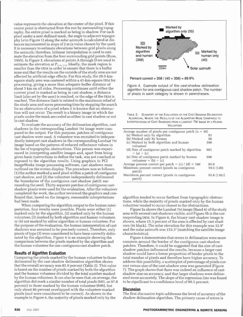
When comparing the algorithm output to the human inter- pretation, four results were possible. Pixels were either (I) marked only by the algorithm, (2) marked only by the human volunteer, (3) marked by both algorithm and human volunteer, or (4) not marked by either algorithm or human volunteer. For the purpose of the evaluation, the human interpretation of cast shadows was assumed to be precisely correct. Therefore, only pixels of type (3) were considered to have been correctly delin- eated by the algorithm. Figure 4 is an example showing the comparison between the pixels marked by the algorithm and the human volunteer for one contiguous cast shadow patch.

Results of Algorithm Evaluation Comparing the pixels marked by the human volunteer to those delineated by the cast-shadow delineation algorithm shows that the overall accuracy was 85.9 percent (Table 2). This value is based on the number of pixels marked by both the algorithm and the human volunteer divided by the total number marked by the human volunteer. It can also be seen that, on average, the algorithm did mark a similar number of total pixels (681, or 97.8 nercentl to those marked bv the human volunteer 16961. but . ,, ~ ~-~

Lnly abbut 86 percent oveGapped with the volunteer-marked pixels (and were considered to be correct). As shown in the example in Figure 4, the majority of pixels marked only by the

Marked by algorithm only (55) L

m Marked by algorithm and human (358)

Percent correct = 358 l (40 + 358) = 89.9%

Figure 4. Example output of the cast-shadow delineation algorithm for one contiguous cast shadow patch. The number of pixels in each category is shown in parentheses.

TABLE 2. SUMMARY OF THE EVALUATION OF THE CAST-SHADOW DELINEATION ALGORITHM, WHERE THE RESULTS OF THE ALGORITHM WERE COMPARED TO

~NTERPRETATION OF CAST SHADOWS FROM A LANOSAT TM IMAGE BY A HUMAN VOLUNTEER

Average number of pixels per contiguous patch [n = (a) Marked only by algorithm [b) Marked only by human (c) Marked by both algorithm and human

volunteer [d) Size of contiguous patch marked by algorithm

= (a) + (c) (e) Size of contiguous patch marked by human

volunteer = (b) + (c) Average percent correct per patch = (c) / (dl x 100 Minimum percent correct (pixels in contiguous

patch) Maximum percent correct (pixels in contiguous

patch)

algorithm tended to occur furthest from topographic obstruc- tions, while the majority of pixels marked only by the human volunteer tended to occur closest to the obstructions.

Figure 5a shows the Landsat TM image (Band 4) of the study area with several cast shadows visible, and Figure 5b is the cor- responding DEM. In Figure 6, the binary cast-shadow image is shown, where 15.3 percent of the area is affected by cast shad- ows (in black). The solar elevation for this example was 32.9" and the solar azimuth was 153.3" (matching the satellite image characteristics).

Figure 4 demonstrates that errors in delineation were more common around the border of the contiguous cast-shadow patches. Therefore, it could be suggested that the size of cast- shadow patches influenced the results, because a larger cast shadow could have a lower proportion of border pixels to the total number of pixels and therefore have higher accuracy. To address this possibility, a scatterplot of percentage of pixels cor- rect versus size of the cast-shadow area was generated (Figure 7). The graph shows that there was indeed an influence of cast- shadow size on accuracy, and that larger shadows were deline- ated more accurately. The slope of the regression line was found to be significant to a confidence level of 99.5 percent.

Discusslon The first discussion topic addresses the level of accuracy of the shadow delineation algorithm. The primary cause of errors is

PHOTOGRAMMETRIC ENGINEERING & REMOTE SENSING

- 2000m

Figure 6. Result of the cast-shadow delineation algorithm for the landscape shown in Figure 5 where black areas repre- sent cast shadows. For this solar position (elevation of 32.g0, azimuth of 153.3"), 15.3 percent of the landscape is marked a s being in cast shadow.

Figure 5. (a) Landsat TM image (Band 4) of the landscape in Kluane National Park Reserve, Yukon. Several cast shad- ows are visible in the lee of mountain peaks and ridges (examples are indicated with arrows). North is towards the top of the image. (0 Space Imaging Corp., received by Can- ada Centre for Remote Sensing, and processed by RADARSAT International.) (b) Digital elevation model of the area shown in Figure 5a. The range of elevation in this image is from 570 m to 2500 m.

likely due to the accuracy (or lack there00 of the DEM in com- parison to the actual landscape. In a situation where a small DEM error can make the difference between a pixel being marked as a shadow or not, the requirements for DEM accuracy

100 -.8 +:* - .

. * $ L * * 5 80 . a, t .* *. 8 60 : C c y = 0.0083~ + 77.2 a, 40 e $ 20

0 0 500 1000 1500 2000

Size of contiguous shadow (pixels)

Figure 7. Scatterplot showing the relationship between accuracy of the cast-shadow delineation algorithm ("Percent correct") and the size of contiguous cast shadow patches. The slope of the regression line is significant to a confidence level of 99.5 percent.

are extreme. The type of DEM used in this study, derived from 1:50,000-scale topographic map contours, is common for this size of study area. During the initial cartographic exercise, scanning, conversion of contours into a grid format, and filter- ing of the DEM, some of the fine topographic details would have been omitted initially or lost subsequently due to interpolation and smoothing. For example, as suggested by the DEM evalua- tion in Figure 2, ridge crests were smoothed with the 3 by 3 low pass filter, reducing the potential for a cast-shadow pixel to be marked correctly where the angle to surrounding topography is similar to the solar elevation angle.

PHOTOGRAMMETRIC ENGINEERING 81 REMOTE SENSING

In addition to the accuracy of the DEM, there are other pos- sible reasons for differences in the size of areas marked by the algorithm and the human volunteer. First, although the author reviewed the work of the human volunteer, a potential source of reduced accuracy lies in the interpretation, particularly close to the edge of the cast-shadow patches where a judge- ment decision was required about precisely which pixels the shadow covered. Second, the registration between the DEM and the satellite image was not perfect, but the average hori- zontal residual error of less than one-pixel was reasonable given the terrain and lack of precise ground control points. The imperfect registration or misalignment between the DEM and the image might cause, falsely, the appearance of marked but non-overlapping pixels that were counted as incorrect. Third, the algorithm might not mark as cast shadow the pixel near the apex of a ridge, because the angle along the azimuth to adja- cent topography is less than the solar elevation angle. Pixels with low reflectance values at ridges that may have been inter- preted as shadows would therefore have been left unmarked by the algorithm.

Overall, based on these results, a caution must be made to workers who rely on automated cast-shadow delineation pro- grams prior to performing exercises such as correcting image values. While in theory it may be valid to assume that topo- graphic features block direct solar radiation from reaching parts of the landscape surface, practical considerations may affect the accuracy of the results, particularly with small cast-shadow patches and, in general, around the edges of patches.

The second topic for discussion considers, in the context of supervised classification, what can be done if a remote sens- ing image contains shadows cast by topography. After delineat- ing cast shadows as accurately as possible, various approaches to dealing with the shadows are possible when classifying images. Recall that, while an analyst may wish to classify simi- lar surfaces in the same logical class, the effect of cast shadows on the reflectance values would complicate this action. One possible approach is to remove pixels marked as cast shadows from consideration in the classification. That is, rather than entering a cast shadow pixel into the classification routine, it could be blocked out and directly assigned a value marking it as cast shadow. In this way, the classification algorithm would be prevented from classifying the pixel correctly, but it would also be prevented from making an error of confusion, such as with lakes as described above. A second (although cumber- some) approach is to set up a classification scheme with dual classes; for example, Ice (In Cast Shadow) and Ice (Not In Cast Shadow). The analyst would then treat the classes separately, including during training. As a post-classification option, the dual classes could be combined into one by recoding (e.g., Ice). A similar multiple-training approach for dealing with illumi- nation variations within classes was discussed by Itten and Meyer (1993).

A third approach for dealing with cast shadows is to attempt a correction to remove the effect of the shadows. Many correction algorithms have a significant drawback for the non- expert image analyst: the algorithms can be daunting in terms of complexity and knowledge requirement, and such algo- rithms often require detailed atmospheric data (e.g., Kawata et aL, 1988; Richter, 1998). Often the required atmospheric parameters are not known or are not feasible to collect during image acquisition. While full-scale atmospheric modeling is desirable for image correction, it is beyond the capabilities of many users of remote sensing images. In contrast, a simpler cor- rection procedure, such as band ratioing (Colby, 1991), may be insufficiently accurate. Preliminary attempts by this author to develop a simple correction for cast shadows by using the rela- tionship between similar paired surfaces (i.e., adjacent similar surfaces in shadow and not in shadow) have so far proven unsuccessful, but are ongoing.

Conclusion Shadows cast by topography interfere with a common assump- tion in the analysis of optical-infrared remote sensing images: that surfaces with similar cover and slope orientation charac- teristics are expected to have similar reflectance values in an image. Not accounting for cast shadows is likely to lead to clas- sification errors when using automated routines. Accounting for cast shadows frequently involves delineating such areas with an automated algorithm and a DEM, but the spatial accu- racy of the cast shadows may be left unquestioned. This article has shown that, in comparison to the interpretation provided by a human volunteer, a cast-shadow delineation algorithm cor- rectly marked 86 percent of the cast-shadow pixels overall.

Acknowledgments Permission to use digital data, given by the Warden Service of Kluane National Park Reserve, is gratefully acknowledged. An evaluation version of OrthoEngine software from PC1 Geomat- ics Group was used to orthogonalize the satellite image. Karen Connolly and Peter Green provided valuable assistance as vol- unteers for image analysis tasks. Two anonymous reviewers are thanked for their contributions to this article.

References Anderson, J.R., E. Hardy, J. Roach, and R. Witmer, 1976. A Land Use

and Land Cover Classification System for Use with Remote Sensor Data, Professional Paper 964, U.S. Geological Survey, Washington, D.C., 28 p.

Brown, D.G., 1991. Topoclimatic models of an alpine environment using digital elevation models within a GIs, Proceedings, GIs/ LIS '91 Conference, 28 October-01 November, Atlanta, Georgia, 2:835-844.

Campbell, J.B., 1996, Introduction to Remote Sensing, Second Edition, Guilford Press, New York, N.Y., 622 p.

Civco, D.L., 1989. Topographic normalization of Landsat Thematic Mapper digital imagery, Photogrammetric Engineering & Remote Sensing, 55(9):1303-1309.

Colby, J.D., 1991. Topographic normalization in rugged terrain, Photo- grammetric Engineering b Remote Sensing, 57(5):531-537.

Crippen, R.E., R.G. Blom, and J.R. Heyada, 1988. Directed band ratioing for the retention of perceptually-independent topoographic expression in chromaticity-enhanced imagery, International Jour- nal of Remote Sensing, 9(4):749-765.

Dozier, J., J. Bruno, and P. Downey, 1981. A faster solution to the horizon problem, Computers and Geosciences, 7(1):145-151.

Frank, T.D., 1988. Mapping dominant vegetation communities in the Colorado Rocky Mountain Front Range with Landsat Thematic Mapper and digital terrain data, Photogrammetric Engineering & Remote Sensing, 54(12):1727-1734.

Guo, L.J., and J. McM. Moore, 1993. Cloud-shadow suppression tech- nique for enhancement of airborne Thematic Mapper imagery, Photogrammetric Engineering b Remote Sensing, 59(8):1287-1291.

Hall-Konyves, K., 1987. The topographic effect on Landsat data in gently undulating terrain in southern Sweden, International Jour- nal of Remote Sensing, 8(2):157-168.

Itten, K.I., and P. Meyer, 1993. Geometric and radiometric correction of TM data of mountainous forested areas, IEEE 'hnsactions on Geoscience and Remote Sensing, 31(4):764-770.

Jensen, J.R., 1996. Introductory Digital Image Processing, Prentice-Hall, Englewood Cliffs, N.J., 316 p.

Kawata, Y., S. Ueno, and T. Kusaka, 1988. Radiometric correction for atmospheric and topographic effects on Landsat MSS images, Internotional Journal of Remote Sensing, 9(4):729-748.

Krishna, A.P., 1996. Satellite remote sensing applications for snow cover characterization in the morphogenetic regions of upper Tista river basin, Sikkim Himalaya, International Journal of Remote Sensing, 17(4):651-656.

PHOTOGRAMMETRIC ENGINEERING & REMOTE SENSING

McGuffie, K., and A. Henderson-Sellers, 1986. Illustration of the influ- Russ, J.C., 1995. The Image Processing Handbook, Second Edition, ence of shadowing on high latitude information derived from CRC Press, Boca Raton, Florida, 674 p. satellite imagery, International Journal of Remote Sensing, Sader, S.A., R.B. Waide, W.T. Lawrence, and A.T. Joyce, 1989. Tropical 7(10):1359-1365. forest biomass and successional age class relationships to a vege-

Pouch, G.W., and D.J. Campagna, 1990. Hyperspherical direction taytion index derived from Landsat TM data, Remote Sensing of cosine transformation for separation of spectral and illumination Environment, 28(1):143-156. information in digital scanner data, Photogmmmetric Engi- Shu, J.S.-P., and H. Freeman, 1990. Cloud shadow removal f?om aerial neering 6. Remote Sensing, 56[4):475-479. photographs, Pattern Recognition, 23(6):647-656.

R.* Correction of Over mountainous Wilson, P.A., 1997. Rule-based classification of water in Landsat MSS terrain, Applied Optics, 3 7(18):4004-4015. images using the variance filter, Photogmmmetric Engineering 6.

Rossi, R.E., J.L. Dungan, and L.R. Beck, 1994. Kriging in the shadows: Remote Sensing, 63(5):485-491. Geostatistical interpolation for remote sensing, Remote Sensing of Environment, 49(1):32-40. (Received 16 June 2000; revised and accepted 31 October 2000)

MAXIMIZE YOUR COMPANY'S EXPOSURE BY HAVING YOUR IMAGES FEATURED I N

ASPRS PROMOTIONAL MATERIALS!

-- As technology Is constantly changing, it is important for the society to provide the most current representations of this industry t o our members, readers, and potential clients o r employees.

We need your help with locating applicable images that convey exceptional examples of the work done by our profession so that w e can expand the variety of images in our photo lmage bank. We are asking all ASPRS Sustaining Members t o participate by do- nating five t o ten of their company's Images illustrating good examples of CIS, Photo- grammetry or Remote Sensing.

The Images would be featured throughout A S P S promotional materials - primarily conference brochures and advertisements, membership pieces, and the ASPRS Career Brochure and accompanying materials.

-

In exchange for your donation, your company will receive photo recognition wherever the image is used, thereby increasing your company's vlslbility. We encourage you t o take advantage of this opportunity-please participate.

To donate images, please follow the submission instructions below. For more information, please contact A S P S Production Manager, Rae Kelley by phone: 301-493-0290 ext.107 or emaii: rkelley@asprs.org.

Submission lnstructions Color 300 DPI, tiff or e p s format 40-50 word description including image type, CIS, Photogrammetry or Remote Sensing Submit on a disk or to the A S P S FTP site {Contact Rae Kelley for logon instructions.)

Thank you in advance for your support1

Donate an lmage today and it may be featured in the ASPRS Career Poster! The poster will accompany the ASPRS Career Brochure and serve a s an additional marketing piece t o help promote the education initiative. The poster will be given t o high school teachers and college pro- fessors teaching subjects relative to our industry.

PHOTOGRAMMETRIC ENGINEERING & REMOTE SENSING fuly 2001 839