Reliability Education Opportunity: “Reliability Analysis of Field Data”

25th Anniversary of Reliability Engineering @ University of Maryland

Vasiliy Krivtsov, PhD Sr. Staff Technical Specialist Reliability & Risk Analysis

Ford Motor Company

2

Discussion Outline

Introduction

Practical Importance of Reliability Analysis of Field Data

Modelling Peculiarities in Reliability Analysis of Field Data

Staggered Production/Sales

Bivariate Models (Time & Usage)

Seasonality

Data Maturation Issues

Illustrative Case Studies

Proposed Course Structure

Conclusions

3

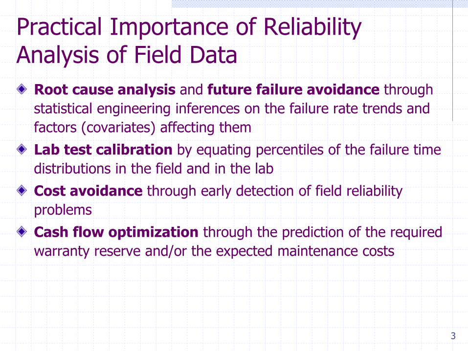
Practical Importance of Reliability Analysis of Field Data

Root cause analysis and future failure avoidance through

statistical engineering inferences on the failure rate trends and

factors (covariates) affecting them

Lab test calibration by equating percentiles of the failure time

distributions in the field and in the lab

Cost avoidance through early detection of field reliability

problems

Cash flow optimization through the prediction of the required

warranty reserve and/or the expected maintenance costs

Staggered Production/Sales

5

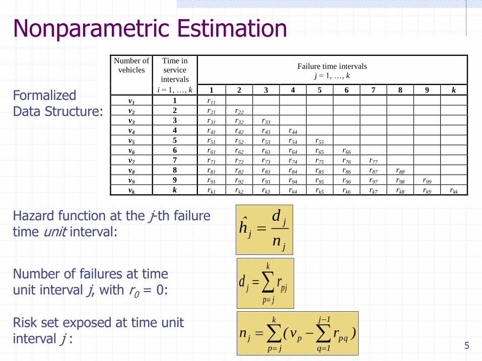
Number of failures at time unit interval j, with r0 = 0:

k

jp

pjj rd

k

jp

1j

1q

pqpj )rv(nRisk set exposed at time unit interval j :

Number of

vehicles

Time in

service

intervals

Failure time intervals

j = 1, …, k

i = 1, …, k 1 2 3 4 5 6 7 8 9 k

v1 1 r11

v2 2 r21 r22

v3 3 r31 r32 r33

v4 4 r41 r42 r43 r44

v5 5 r51 r52 r53 r54 r55

v6 6 r61 r62 r63 r64 r65 r66

v7 7 r71 r72 r73 r74 r75 r76 r77

v8 8 r81 r82 r83 r84 r85 r86 r87 r88

v9 9 r91 r92 r93 r94 r95 r96 r97 r98 r99

vk k rk1 rk2 rk3 rk4 rk5 rk6 rk7 rk8 rk9 rkk

Nonparametric Estimation

Formalized Data Structure:

j

j

jn

dh

Hazard function at the j-th failure time unit interval:

6

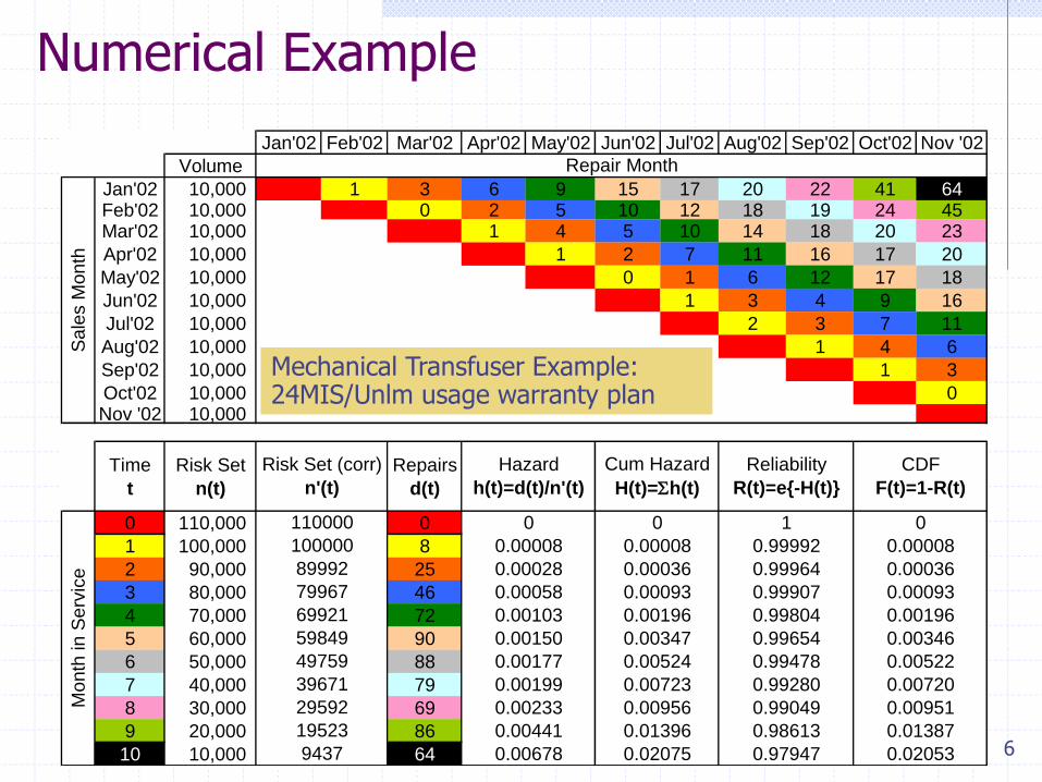
Numerical Example

Jan'02 Feb'02 Mar'02 Apr'02 May'02 Jun'02 Jul'02 Aug'02 Sep'02 Oct'02 Nov '02

Volume

Jan'02 10,000 1 3 6 9 15 17 20 22 41 64Feb'02 10,000 0 2 5 10 12 18 19 24 45Mar'02 10,000 1 4 5 10 14 18 20 23

Apr'02 10,000 1 2 7 11 16 17 20

May'02 10,000 0 1 6 12 17 18

Jun'02 10,000 1 3 4 9 16

Jul'02 10,000 2 3 7 11

Aug'02 10,000 1 4 6

Sep'02 10,000 1 3

Oct'02 10,000 0Nov '02 10,000

Time

t

Risk Set

n(t)

Repairs

d(t)

0 110,000 0

1 100,000 8

2 90,000 25

3 80,000 46

4 70,000 72

5 60,000 90

6 50,000 88

7 40,000 79

8 30,000 69

9 20,000 86

10 10,000 64

29592

19523

9437

69921

59849

49759

39671

110000

100000

89992

79967

0.01396

0.00956

CDF

F(t)=1-R(t)

Cum Hazard

H(t)=Sh(t)

0.99907

0.99964

0.99992

01

0.00720

0.00951

0.01387

0.02053

Repair Month

0.99804

0.99654

0.99478

0.00008

0.00036

0.00093

0.00196

0.00346

0.00522

0.00036

0.00093

0.00196

0.00347

0.00524

0.007230.00199

0.00233

0.00441

0.00678

0.99280

0.99049

0.98613

0.979470.02075

Reliability

R(t)=e{-H(t)}

Mo

nth

in

Se

rvic

e

0

0.00008

0.00028

0.00058

0.00103

0.00150

0.00177

0

Sale

s M

onth

Hazard

h(t)=d(t)/n'(t)

Risk Set (corr)

n'(t)

0.00008

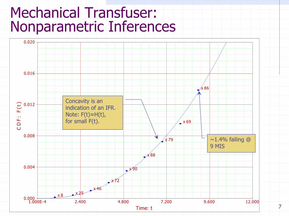
Mechanical Transfuser Example: 24MIS/Unlm usage warranty plan

7 Time: t

CD

F: F

(t)

1.000E-4 12.0002.400 4.800 7.200 9.6000.000

0.020

0.004

0.008

0.012

0.016

x 8x 25

x 46

x 72

x 90

x 88

x 79

x 69

x 86

Mechanical Transfuser: Nonparametric Inferences

~1.4% failing @ 9 MIS

Concavity is an indication of an IFR. Note: F(t)≈H(t), for small F(t).

8

j

k

jp

j

q

jpqpj rvn1

1

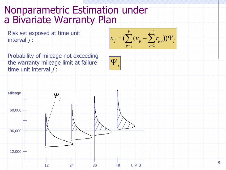
))((Risk set exposed at time unit interval j :

Probability of mileage not exceeding the warranty mileage limit at failure time unit interval j :

Nonparametric Estimation under a Bivariate Warranty Plan

12 24 36 48 t, MIS

12,000

36,000

60,000

Mileage

j

9

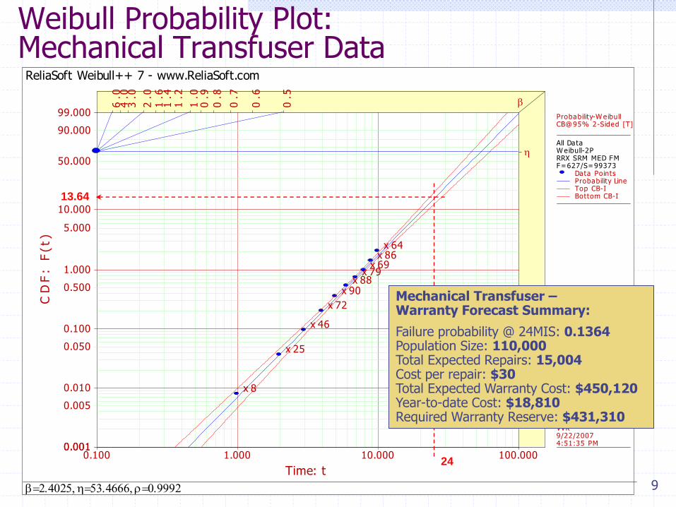
Weibull Probability Plot: Mechanical Transfuser Data ReliaSoft Weibull++ 7 - www.ReliaSoft.com

Time: t

CD

F: F

(t)

0.100 100.0001.000 10.0000.001

0.005

0.010

0.050

0.100

0.500

1.000

5.000

10.000

50.000

90.000

99.000

0.001

x 8

x 25

x 46

x 72

x 90x 88

x 79x 69

x 86x 64

0.5

0.6

0.7

0.8

0.9

1.0

1.2

1.4

1.6

2.0

3.0

4.0

6.0

Probability-W eibullCB@ 95% 2-Sided [T]

All DataW eibull-2PRRX SRM MED FMF=627/S=99373

Data PointsProbability LineTop CB-IBottom CB-I

Vasiliy KrivtsovVVK9/22/20074:51:35 PM

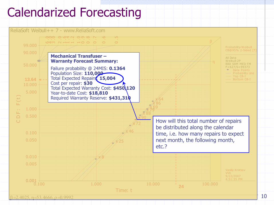
Mechanical Transfuser – Warranty Forecast Summary:

Failure probability @ 24MIS: 0.1364 Population Size: 110,000 Total Expected Repairs: 15,004 Cost per repair: $30 Total Expected Warranty Cost: $450,120 Year-to-date Cost: $18,810 Required Warranty Reserve: $431,310

13.64

24

10

Calendarized Forecasting

ReliaSoft Weibull++ 7 - www.ReliaSoft.com

Time: t

CD

F: F

(t)

0.100 100.0001.000 10.0000.001

0.005

0.010

0.050

0.100

0.500

1.000

5.000

10.000

50.000

90.000

99.000

0.001

x 8

x 25

x 46

x 72

x 90x 88

x 79x 69

x 86x 64

0.5

0.6

0.7

0.8

0.9

1.0

1.2

1.4

1.6

2.0

3.0

4.0

6.0

Probability-W eibullCB@ 95% 2-Sided [T]

All DataW eibull-2PRRX SRM MED FMF=627/S=99373

Data PointsProbability LineTop CB-IBottom CB-I

Vasiliy KrivtsovVVK9/22/20074:51:35 PM

13.64

24

Mechanical Transfuser – Warranty Forecast Summary:

Failure probability @ 24MIS: 0.1364 Population Size: 110,000 Total Expected Repairs: 15,004 Cost per repair: $30 Total Expected Warranty Cost: $450,120 Year-to-date Cost: $18,810 Required Warranty Reserve: $431,310

How will this total number of repairs be distributed along the calendar time, i.e. how many repairs to expect next month, the following month, etc.?

11

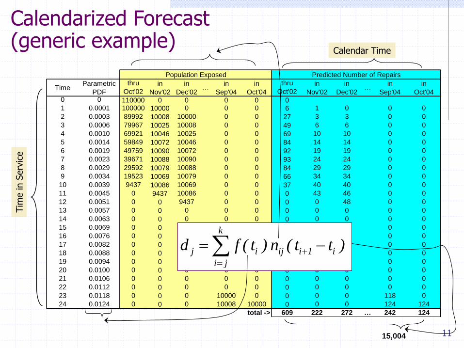
TimeParametric

PDF

thru

Oct'02in

Nov'02

in

Dec'02…

in

Sep'04

in

Oct'04

thru

Oct'02in

Nov'02

in

Dec'02…

in

Sep'04

in

Oct'040 0 110000 0 0 0 0 01 0.0001 100000 10000 0 0 0 6 1 0 0 0

2 0.0003 89992 10008 10000 0 0 27 3 3 0 0

3 0.0006 79967 10025 10008 0 0 49 6 6 0 0

4 0.0010 69921 10046 10025 0 0 69 10 10 0 0

5 0.0014 59849 10072 10046 0 0 84 14 14 0 0

6 0.0019 49759 10090 10072 0 0 92 19 19 0 0

7 0.0023 39671 10088 10090 0 0 93 24 24 0 0

8 0.0029 29592 10079 10088 0 0 84 29 29 0 0

9 0.0034 19523 10069 10079 0 0 66 34 34 0 0

10 0.0039 9437 10086 10069 0 0 37 40 40 0 0

11 0.0045 0 9437 10086 0 0 0 43 46 0 0

12 0.0051 0 0 9437 0 0 0 0 48 0 0

13 0.0057 0 0 0 0 0 0 0 0 0 0

14 0.0063 0 0 0 0 0 0 0 0 0 0

15 0.0069 0 0 0 0 0 0 0 0 0 0

16 0.0076 0 0 0 0 0 0 0 0 0 0

17 0.0082 0 0 0 0 0 0 0 0 0 0

18 0.0088 0 0 0 0 0 0 0 0 0 0

19 0.0094 0 0 0 0 0 0 0 0 0 0

20 0.0100 0 0 0 0 0 0 0 0 0 0

21 0.0106 0 0 0 0 0 0 0 0 0 0

22 0.0112 0 0 0 0 0 0 0 0 0 0

23 0.0118 0 0 0 10000 0 0 0 0 118 0

24 0.0124 0 0 0 10008 10000 0 0 0 124 124

609 222 272 … 242 124

Population Exposed Predicted Number of Repairs

total ->

Calendarized Forecast (generic example)

k

ji

i1iijij )tt(n)t(fd

Calendar Time

Tim

e in S

erv

ice

15,004

Time vs. Usage

13

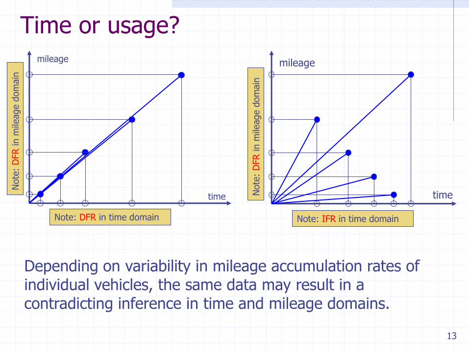
Time or usage?

time

mileage

time

mileage

Note: DFR in time domain Note: IFR in time domain

Note

: D

FR in m

ileage d

om

ain

Note

: D

FR in m

ileage d

om

ain

Depending on variability in mileage accumulation rates of individual vehicles, the same data may result in a contradicting inference in time and mileage domains.

14

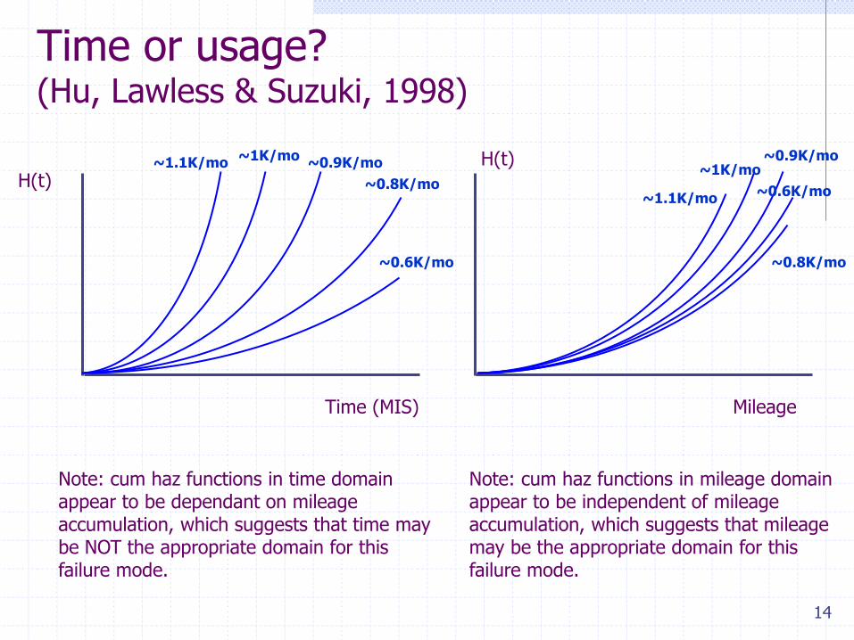
Time or usage? (Hu, Lawless & Suzuki, 1998)

Time (MIS)

H(t) ~1.1K/mo

~1K/mo

~0.8K/mo

~0.9K/mo

~0.6K/mo

Note: cum haz functions in time domain appear to be dependant on mileage accumulation, which suggests that time may be NOT the appropriate domain for this failure mode.

Mileage

H(t)

~1.1K/mo

~1K/mo

~0.8K/mo

~0.9K/mo

~0.6K/mo

Note: cum haz functions in mileage domain appear to be independent of mileage accumulation, which suggests that mileage may be the appropriate domain for this failure mode.

15

Time or usage? (Kordonsky & Gertsbakh, 1997)

Time (MIS)

f(t)

Choose the scale that provides a lower coefficient of variation of the respective failure distribution.

Mileage

f(t)

Data Maturity

17

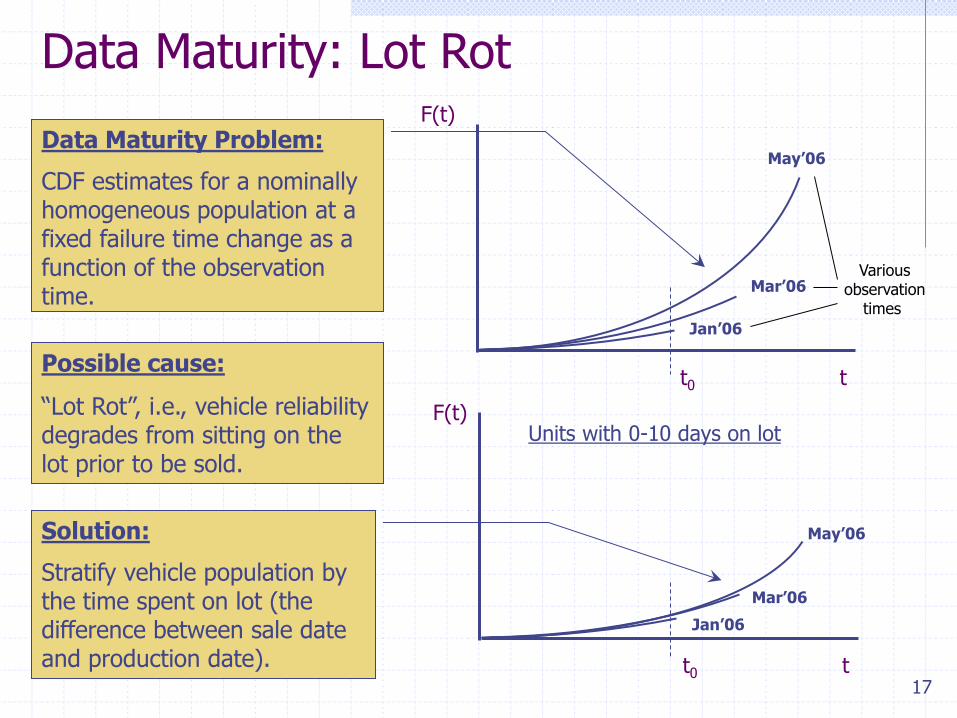
Data Maturity: Lot Rot

t

F(t)

Jan’06

Mar’06

May’06

t0

Data Maturity Problem:

CDF estimates for a nominally homogeneous population at a fixed failure time change as a function of the observation time.

Possible cause:

“Lot Rot”, i.e., vehicle reliability degrades from sitting on the lot prior to be sold.

Various observation

times

Solution:

Stratify vehicle population by the time spent on lot (the difference between sale date and production date). t

F(t)

Jan’06

Mar’06

May’06

t0

Units with 0-10 days on lot

18

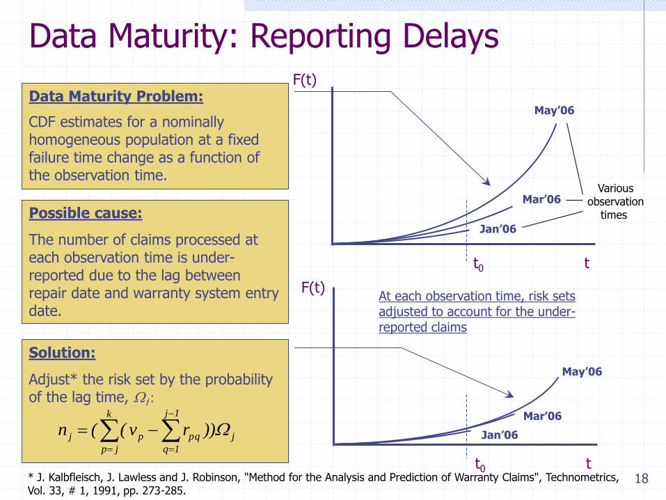
Data Maturity: Reporting Delays

t

F(t)

Jan’06

Mar’06

May’06

t0

Data Maturity Problem:

CDF estimates for a nominally homogeneous population at a fixed failure time change as a function of the observation time.

Possible cause:

The number of claims processed at each observation time is under-reported due to the lag between repair date and warranty system entry date.

Various observation

times

Solution:

Adjust* the risk set by the probability of the lag time, Wj:

t

F(t)

Jan’06

Mar’06

May’06

t0

At each observation time, risk sets adjusted to account for the under-reported claims

k

jp

1j

1q

jpqpj ))rv((n W

* J. Kalbfleisch, J. Lawless and J. Robinson, "Method for the Analysis and Prediction of Warranty Claims", Technometrics, Vol. 33, # 1, 1991, pp. 273-285.

19

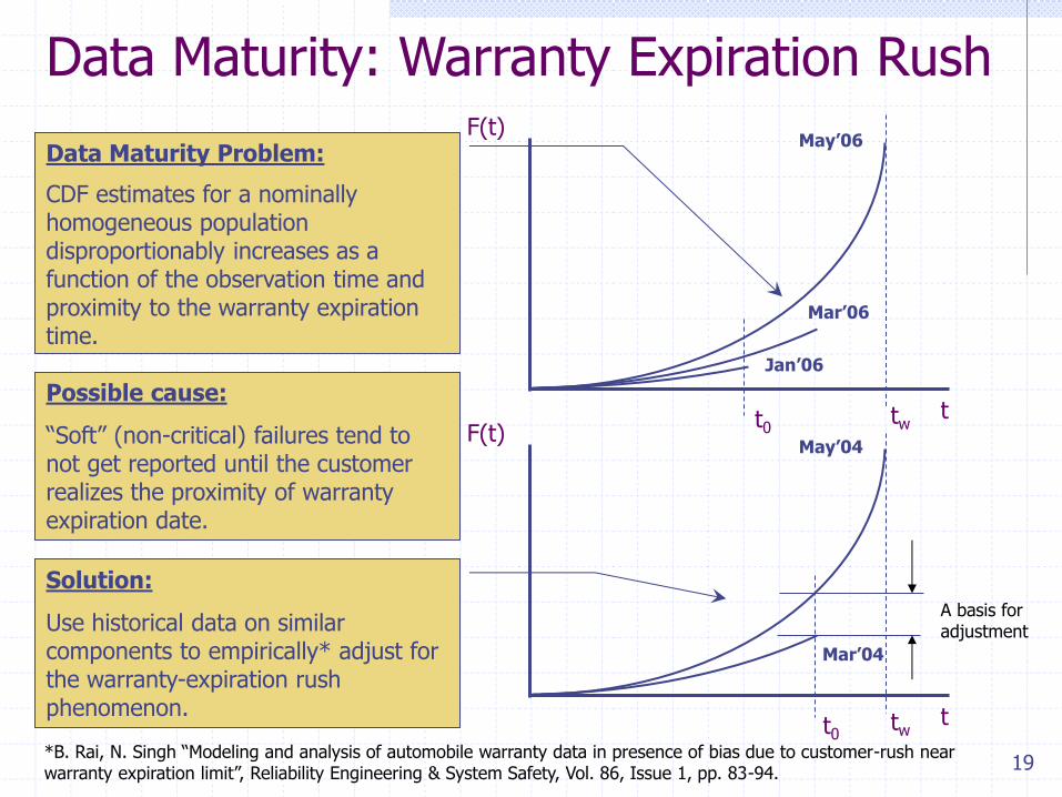
Data Maturity: Warranty Expiration Rush

t

F(t)

Jan’06

Mar’06

May’06

t0

Data Maturity Problem:

CDF estimates for a nominally homogeneous population disproportionably increases as a function of the observation time and proximity to the warranty expiration time.

Possible cause:

“Soft” (non-critical) failures tend to not get reported until the customer realizes the proximity of warranty expiration date.

Solution:

Use historical data on similar components to empirically* adjust for the warranty-expiration rush phenomenon.

*B. Rai, N. Singh “Modeling and analysis of automobile warranty data in presence of bias due to customer-rush near warranty expiration limit”, Reliability Engineering & System Safety, Vol. 86, Issue 1, pp. 83-94.

tw

t

F(t)

Mar’04

May’04

t0 tw

A basis for adjustment