Reliability analysis for preventive maintenance based on classical andBayesian semi-parametric degradation approaches using locomotivewheel-sets as a case study

Jing Lin a,b,n, Julio Pulido c, Matthias Asplund a,d

a Division of Operation and Maintenance Engineering, Luleå University of Technology, 97187 Luleå, Swedenb Luleå Railway Research Centre, 97187 Luleå, Swedenc ReliaSoft Corporation, Tucson, AZ 85710-6703, USAd Swedish Transport Administration, 97125 Luleå, Sweden

a r t i c l e i n f o

Article history:Received 18 August 2013Received in revised form7 October 2014Accepted 8 October 2014Available online 28 October 2014

Keywords:ReliabilityPreventive maintenanceDegradation modelsAccelerate life testingBayesian approach

a b s t r a c t

This paper undertakes a general reliability study using both classical and Bayesian semi-parametricdegradation approaches. The goal is to illustrate how degradation data can be modelled and analysed toflexibly determine reliability to support preventive maintenance strategy making, based on a generaldata-driven framework. With the proposed classical approach, both accelerated life tests (ALT) anddesign of experiments (DOE) technology are used to determine how each critical factor affects theprediction of performance. With the Bayesian semi-parametric approach, a piecewise constant hazardregression model is used to establish the lifetime using degradation data. Gamma frailties are included toexplore the influence of unobserved covariates within the same group. Ideally, results from the classicaland Bayesian approaches will complement each other. To demonstrate these approaches, this paperconsiders a case study of locomotive wheel-set reliability. The degradation data are prepared byconsidering an Exponential and a Power degradation path separately. The results show that bothclassical and Bayesian semi-parametric approaches are useful tools to analyse degradation data and can,therefore, support a company in decision making for preventive maintenance. The approach can beapplied to other technical problems (e.g. other industries, other components).

& 2014 Elsevier Ltd. All rights reserved.

1. Introduction

Estimating the failure-time distribution or long-term perfor-mance of components of high reliability products is particularlydifficult. Many modern products are designed to operate withoutfailure for a long time, for example, train wheel-sets. Thus, fewunits will fail or significantly degrade in a test of practical length atnormal use conditions.

The service life of train wheel-sets can be significantly reduceddue to failure or damage, leading to excessive cost and accelerateddeterioration, a point which has received considerable attention inrecent literature. In order to monitor the performance of wheel-setsand make replacements in a timely fashion, the railway industry usesboth preventive and predictive maintenance. By predicting the wear[14,2,29], fatigue [1,17], tribological aspects [5], and failures [31],

the industry can design strategies for different types of preventivemaintenance (re-profiling, lubrication, etc.) for various periods (days,months, seasons, running distance, etc.). Software dedicated topredicting wear rate has also been proposed [22]. Finally, conditionmonitoring data have been studied with a view to increasing thewheel-sets’ lifetime [25,8,28,21].

Preventive maintenance (PM) actions are usually performed atpredetermined points in time to keep the reliability of the systemat a desired level [9]. One common preventive maintenancestrategy (used in the case study) is re-profiling wheel-sets afterthey run a certain distance. Re-profiling affects the wheel’sdiameter; once the diameter is reduced to a pre-specified length,the wheel-set is replaced by a new one. Seeking to optimise thismaintenance strategy, researchers have examined wheel-setdegradation data to determine wheel-set reliability and failuredistribution. However, in previous studies, some researchers havenoticed that the wheel-sets’ different installed positions mayinfluence the results. To avoid this possibility, Freitas et al. [11]only consider those wheels on the left side of a specified axleand on certain specified cars, arguing that “the degradation of a

Contents lists available at ScienceDirect

journal homepage: www.elsevier.com/locate/ress

Reliability Engineering and System Safety

http://dx.doi.org/10.1016/j.ress.2014.10.0110951-8320/& 2014 Elsevier Ltd. All rights reserved.

n Corresponding author.E-mail addresses: janet.lin@ltu.se (J. Lin), Julio.pulido@reliasoft.com (J. Pulido),

Matthias.asplund@ltu.se (M. Asplund).

Reliability Engineering and System Safety 134 (2015) 143–156

given wheel might be associated with its position on a given car”.Yang and Letourneau [31] suggest certain attributes, including awheel's installed position (right or left), might influence its wearrate, but they do not provide case studies. Palo [21] conclude that“different wheel positions in a bogie show significantly differentforce signatures”. Recently, to solve the combined problem of smalldata samples and incomplete datasets whilst simultaneously con-sidering the influence of several covariates, Lin et al. [16] haveexplored the influence of locomotive wheels’ positioning on relia-bility with Bayesian parametric models. Their results indicate thatthe particular bogie in which the wheel is mounted has moreinfluence on its lifetime than does the axle or which side it is on. Asthis paper is an extension of the study in Lin et al. [16], in additionto the locomotive, we only use the bogie as a main influence factor.

To achieve complementary results, we perform a reliabilitystudy using both classical and Bayesian semi-parametric frame-works and propose a general data-driven framework. In the casestudy, we explore the impact of a locomotive wheel-set’s positionon its service lifetime to predict its other reliability characteristics.The goal is to illustrate how a wheel-set’s degradation data can bemodelled and analysed using both classical and Bayesianapproaches in order to flexibly determine reliability for preventivemaintenance strategy making based on the proposed frameworks.Notably, this data-driven method [33] can be extended to otherapplications.

The remainder of the paper is organised as follows. Section 2presents the degradation models using a classical approach. We useboth accelerated life tests (ALT) and design of experiments (DOE)technology to determine how each critical factor affects the predic-tion of performance. Section 3 presents the piecewise constanthazard regression model with gamma frailties. In the proposedmodel, a discrete-time martingale process is considered as a priorprocess for the baseline hazard rate. It adopts a Markov Chain MonteCarlo (MCMC) computational scheme. Section 4 proposes a generaldata-driven framework as a summary and Section 5 describes thecase study of the wheel-sets on two locomotives in a heavy haulcargo train, using both exponential and power degradation assump-tions, and discusses maintenance strategies for optimisation. Finally,Section 6 offers conclusions and comments.

2. Classical approach

In this section, we use a general log linear (GLL) life stressrelationship to analyse the degradation data with accelerated lifetests (ALT), considering lifetime data from a specific degradationpath. Then, using the specific degradation model, we perform atwo factor full factorial design of experiments analysis.

2.1. Accelerated life testing

As discussed above, many modern products are designed tooperate without failure for a long time. Under such conditions, fewunits will fail or significantly degrade in a test of practical length atnormal use conditions. For this reason, accelerated life tests (ALTs)are widely used in manufacturing industries, particularly to obtaintimely information on the reliability of product components andmaterials. Generally, information from tests at high stress levels ofaccelerating variables (e.g., use rate, temperature, voltage, orpressure) is extrapolated, through a physically reasonable statisticalmodel (e.g. Eiren, Arrhenius, Inverse Power Law), to obtain esti-mates of life or long-term performance at lower and normal useconditions. ALT results are used in design-for reliability processes toassess or demonstrate component and subsystem reliability, certifycomponents, detect failure modes, compare manufacturers, and soforth. ALTs have become increasingly important because of rapidly

changing technologies, more complicated products with morecomponents, and higher customer expectations of better reliability.

In some reliability studies, it is possible to measure degradationdirectly over time, either continuously or at specific points in time.In most reliability testing applications, degradation data, if available,can have important practical advantages [15]: particularly inapplications where few or no failures are expected, they can provideconsiderably more reliability information than would be availablefrom traditional censored failure-time data. Accelerated tests arecommonly used to obtain reliability test information more quickly.Direct observation of the degradation process (e.g., tire wear) mayallow direct modelling of the failure-causing mechanism, providingmore credible and precise reliability estimates and a valid basis forextrapolation. Modelling degradation of the performance output ofa component or subsystem (e.g., voltage or power) may be useful,but modelling could be complicated or difficult because the outputmay be affected, albeit unknowingly, by more than one physical/chemical failure-causing process.

Once we obtain the projected failures values for each degrada-tion model, we can carry out an accelerated life analysis usingsome critical factors as stress factors. The analysis can be per-formed using a general log linear (GLL) life stress relationship witha Weibull probability function, modelled as:

LðX Þ ¼ eðα0 þ∑mi ¼ 1αiXiÞ ð2:1Þ

This model (2.1) can also be expressed as an exponential model,with life as a function of the stress vector X, where X is a vector of nstressors [18]. For this analysis, we consider stress applicationsof the model and a logarithmic transformation on X, such thatX ¼ lnðVÞ where V is the specific stress. This transformationgenerates an inverse power model life stress relationship, as shownbelow for each stress factor:

LðVÞ ¼ 1KVn ð2:2Þ

2.2. Design of experiments analysis

Design of experiment (DOE) analysis has been widely appliedto improving product performance [10], as for example, in numer-ous recent reliability studies: DOE makes it possible to exploremultiple stressors in an efficient way for reliability improvementconsidering the no fault found (NFF) phenomenon [26];a two-level full factorial DOE may identify the reliability of thereverse link as the performance metric of real-time traffic [12];a DOE based parameter tuning is proposed to provide an estima-tion of turbine power plant availability [3]; a two factorial DOEanalysis based on the cost associated with maintenance andreplacement activities and reliability characteristic parameters isused to determine the optimal preventive maintenance andreplacement schedules in repairable and maintainable systems[19]; a two-level, three-factor experiment is used to collect humanperformance data under different mustering conditions [20].

Reliability DOE (R-DOE) can be used to identify factors affectingproduct life and can also be used to optimise design variables toimprove product reliability [23]. It is fairly similar to the analysis ofother designed experiments except the response is the life of theproduct in the respective units (e.g., for an automobile component,the units of life may be miles, for a mechanical component thismay be cycles, and for a pharmaceutical product, this may bemonths or years). Note: In Section 5.3, we perform a two factor fullfactorial R-DOE analysis.

J. Lin et al. / Reliability Engineering and System Safety 134 (2015) 143–156144

3. Bayesian semi-parametric approach

Most reliability studies are implemented under the assumptionthat individual lifetimes are independent identically distributed (i.i.d).At times, however, Cox proportional hazard (CPH) models cannot beused because of the dependence of data within a group. For instance,because they have the same operating conditions, the wheel-setsmounted on a particular locomotive may be dependent. In a differentcontext, some data may come from multiple records which actuallybelong to wheel-sets installed in the same position but on anotherlocomotive. Modelling dependence in multivariate survival data hasreceived considerable attention in cases where the datasets maycome from subjects of the same group which are related to each otherin some fashion. A key development in modelling such data is toconsider frailty models, in which the data are conditionally indepen-dent. When frailties are considered, the dependence within sub-groups can be considered an unknown and unobservable risk factor(or explanatory variable) of the hazard function. In this section, weconsider a gamma shared frailty, first discussed by Clayton [4] andlater developed by Sahu et al. [24], to explore the influence ofunobserved covariates. In addition, since semi-parametric Bayesianmethods offer a more general modelling strategy with fewer assump-tions, we adopt the piecewise constant hazard model to establish thedistribution of the lifetime. The applied hazard function is sometimescalled a piecewise exponential model (PEM; [7]); it is convenientbecause it can accommodate various shapes of the baseline hazardover the intervals. This model can also be viewed as a nonparametricALT model [32].

3.1. Piecewise constant hazard regression model

The piecewise constant hazard model is one of the mostconvenient and popular semi-parametric models in survival ana-lysis. We begin by denoting the jth individual in the ith group ashaving lifetime tij, where i¼ 1;…;n and j¼ 1;…;mi. Divide thetime axis into intervals 0os1os2o⋯osko1, where sk4tij,thereby obtaining k intervals ð0; s1�; ðs1; s2�;… ðsk�1; sk�. Supposethe jth individual in the ith group has a constant baseline hazardh0ðtijÞ ¼ λk as in the kth interval, where tijA Ik ¼ ðsk�1; sk�. Then, thehazard rate function for the piecewise constant hazard model canbe written as

h0ðtijÞ ¼ λk; tijA Ik ð3:1Þ

Eq. (3.1) is sometimes referred to as a piecewise exponentialmodel (PEM); it can accommodate various shapes of the baselinehazard over the intervals.

Ref. [7] summarise studies on how to divide the time axis intokintervals. However, using common cutpoints simplifies both thenotation and the ease of understanding the ideas [6]. In this paper,we discuss the choice of k in the case study.

Suppose xi ¼ ðx1i;⋯xpiÞ0 denotes the covariate vector for theindividuals in the ithgroup, and β is the regression parameter.Therefore, the regression model with the piecewise constanthazard rate can be written as

hðtijÞ ¼

λ1expðx0ijβÞ 0otijrs1

λ2expðx0ijβÞ s1otijrs2

⋮ ⋮λkexpðx0

ijβÞ sk�1otijrsk

8>>>><>>>>:

ð3:2Þ

Its corresponding probability density function f ðtijÞ, cumulativedistribution function FðtijÞ, reliability function RðtijÞ, together withthe cumulative hazard rate ΛðtijÞ, can now be achieved.

3.2. Gamma shared frailty model

Frailty models were first considered by Clayton [4] to handlemultivariate survival data. In these models, the event times areconditionally independent according to a given frailty factor, anindividual random effect. As discussed by Sahu et al. [24], themodels formulate different variabilities and come from two dis-tinct sources. The first source is natural variability, explained bythe hazard function; the second is variability common to indivi-duals of the same group or variability common to several events ofan individual, explained by the frailty.

Assume the hazard function for the jth individual in the ithgroup is

hijðtÞ ¼ h0ðtÞexpðμiþx0ijβÞ ð3:3Þ

In Eq. (3.3), μirepresents the frailty parameter for the ith group.By denoting ωi ¼ expðμiÞ, the equation can be written as

hijðtÞ ¼ h0ðtÞωiexpðx0ijβÞ ð3:4Þ

Eq. (3.3) is an additive frailty model, and Eq. (3.4) is a multi-plicative frailty model. In both equations, μiand ωi are shared by theindividuals in the same group; they are thus referred to as shared-frailty models and are actually extensions of the CPH model.

To this point, discussions of frailty models have focused on thechoices of the form of the baseline hazard function and the form ofthe frailty’s distribution. Wienke [30] explores different frailtymodels from both univariate and multivariate perspectives. In thispaper, we consider the piecewise constant hazard rate due to itsflexibility, as well as the gamma shared frailty model, the mostpopular model for frailty.

From Eq. (3.4), suppose the frailty parametersωiare indepen-dent and identically distributed (i.i.d) for each group and follow agamma distribution, denoted by Gaðκ�1; κ�1Þ. In this case, theprobability density function can be written as

f ðωiÞ ¼ðκ�1Þκ � 1

Γðκ�1Þ Uωκ � 1 �1i expð�κ�1ωiÞ ð3:5Þ

In Eq. (3.5), the mean value of ωi is 1, where κ is the unknownvariance ofωis. Greater values of κsignify a closer positive relation-ship between the subjects of the same group, as well as greaterheterogeneity among groups. Furthermore, as ωi41, the failuresfor the individuals in the corresponding group will appear earlierthan if ωi¼1; in other words, asωio1, their predicted lifetimeswill be greater than those found in the independent models.

Suppose ω¼ ðω1;ω2;⋯;ωnÞ0; then

πðω κj Þp ∏n

i ¼ 1ωκ � 1 �1i expð�κ�1ωiÞ ð3:6Þ

3.3. Discrete-time martingale process for baseline hazard rate

Based on the above discussion (Eqs. (3.2), (3.4), and (3.5)), thepiecewise constant hazard model with gamma shared frailties canbe written as:

hðtijÞ ¼

λ1ωiexpðx0ijβÞ 0otijrs1

λ2ωiexpðx0ijβÞ s1otijrs2

⋮ ⋮λkωiexpðx0

ijβÞ sk�1otijrsk

8>>>><>>>>:

ð3:7Þ

In Eq. (3.7), ωi�Gaðκ�1; κ�1Þ.

J. Lin et al. / Reliability Engineering and System Safety 134 (2015) 143–156 145

To analyse the baseline hazard rate λk, a common choice is toconstruct an independent incremental process, e.g., the Gammaprocess, the Beta process, or the Dirichlet process. However, aspointed out by Ibrahim et al. [13], in many applications, priorinformation is often available on the smoothness of the hazardrather than the actual baseline hazard itself. In addition, given thesame covariates, the ratio of marginal hazards at the nearby time-points is approximately equal to the ratio of the baseline hazardsat these points. In such situations, correlated prior processes forthe baseline hazard can be more suitable. Such models, forinstance, the discrete-time martingale process for the baselinehazard rate λk, are discussed by Sahu et al. [24].

Given (λ1; λ2;⋯; λk�1), we specify that

λk λ1; λ2;⋯; λk�1�� � Ga αk;

αkλk�1

� �ð3:8Þ

Let λ0 ¼ 1. In Eq. (3.8), the parameter αkrepresents the smooth-ness for the prior information. If αk ¼ 0, then λk and λk�1 areindependent. Asαk-1, the baseline hazard is the same in thenearby intervals. In addition, the Martingaleλk’s expected value atany time point is the same, and

Eðλk λ1; λ2;⋯; λk�1�� Þ ¼ λk�1 ð3:9Þ

Eq. (3.9) shows that given specified historical informationðλ1; λ2;⋯; λk�1Þ, the expected value of λk is fixed.

3.4. Bayesian semi-parametric model using MCMC

In reliability analysis, the lifetime data are usually incomplete, andonly a portion of the individual lifetimes are known. Right-censoreddata are often called Type I censoring, and the corresponding

likelihood construction problem is extensively studied in the literature.Suppose the jth individual in the ith group has lifetime Tij andcensoring time Lij. The observed lifetimetij ¼ minðTij; LijÞ; therefore,the exact lifetime Tij will be observed only if TijrLij. In addition, thelifetime data involving right censoring can be represented by n pairs ofrandom variables ðtij; υijÞ, where υij ¼ 1 if TijrLij and υij ¼ 0if Tij4Lij.This means that υij indicates whether lifetime Tijis censored or not.The likelihood function is deduced as

LðtÞ ¼ ∏n

i ¼ 1∏mi

j ¼ 1½f ðtijÞ�υij RðtijÞ1� υij ð3:10Þ

In the above piecewise constant hazard model, we denote gij astijAðsgij ; sgij þ1Þ ¼ Igij þ1 and the model's dataset as D¼ ðω;t;X;υÞ.Following Eqs. (3.7)–(3.10), the complete likelihood functionLðβ;λ Dj Þ for the individuals for the ith group in k intervals can bewritten as

∏n

i ¼ 1∏mi

j ¼ 1½ ∏

gij

k ¼ 1expð�λkωiexpðx0

ijβÞðsk�sk�1Þ�(

�ðλgij þ1ωiexpðx0ijβÞÞυij � exp½�λgij þ1ωiexpðx0

ijβÞðtij�sgij Þ�o

ð3:11Þ

Let πðU Þ denote the prior or posterior distributions for theparameters. Following Eqs. (3.6) and (3.11), the joint posteriordistribution πðωi β;λ;D

�� Þ for gamma frailties ωi can be written as

πðωi β;λ;D�� ÞpLðβ; λ Dj Þ � πðω κj Þ

pω

κ � 1 þ ∑mi

j ¼ 1υij�1

i exp �ðκ�1þ½ ∑mi

j ¼ 1expðx0

ijβÞ�Þ(

Fig. 4.1. A general data-driven framework.

J. Lin et al. / Reliability Engineering and System Safety 134 (2015) 143–156146

�ð ∑gij

k ¼ 1λkðsk�sk�1Þþλgij þ1ðtij�sgij ÞÞ

)

� Ga κ�1þ ∑mi

j ¼ 1υij; κ

�1þ½ ∑mi

j ¼ 1expðx0

ijβÞ�ð ∑gij

k ¼ 1λkðsk�sk�1Þ

(

þλgij þ1ðtij�sgij ÞÞo

ð3:12Þ

Eq. (3.12) shows that the full conditional density of each ωi is agamma distribution. Similarly, the full conditional density of κ�1

and β can be given by

πðκ�1 β;ω;λ;D�� Þp ∏

n

i ¼ 1ωκ � 1 �1i ðκ�1Þ�nκ � 1

� exp �κ�1∑ni ¼ 1ωi

� �½Γðκ�1Þ�n Uπðκ�1Þ ð3:13Þ

πðβ κ�1;ω; λ;D�� Þpexp ∑

n

i ¼ 1∑mi

j ¼ 1υijx0

ijβ� ∑n

i ¼ 1∑ni

m ¼ 1expðx0

ijβÞωi

(

� ∑gij

k ¼ 1λkðsk�sk�1Þþλgij þ1ðtij�sgij Þ

" #)� πðβÞ ð3:14Þ

Let Rk ¼ fði; jÞ; tij4skg denote the risk set at sk and Dk ¼ Rk�1�Rk; let dk denote the failure individuals in the intervalIk.Let πðλkjλð�kÞ:Þdenote the conditional prior distribution for(λ1;λ2;⋯; λJ) withoutλk. We therefore derive πðλk β;ω; κ�1;D

�� Þ as

λdkk exp �λkωiexpðx0ijβÞ � ½ ∑

ði;jÞARk

ðsk�sk�1Þþ ∑ði;jÞADk

ðtij�sk�1Þ�( )

� πðλk λð�kÞ��� Þ

ð3:15Þ

Table 5.1Degradation data of Locomotive 1.

Distance (km) Degradation (mm)

Bogie I Bogie II

1 2 3 4 5 6 7 8 9 10 11 12

106613 13.08 13.19 12.11 12.12 12.99 13.04 13.02 13.01 11.94 12.01 13.01 13.16144207 27.11 27.07 23.01 22.86 25.03 25.09 24.09 24.12 23.95 24.06 26.56 26.55191468 38.95 38.94 39.11 39.06 39.15 39.17 35.95 35.95 35.88 35.93 36.24 36.04272697 70.6 70.53 69.94 69.87 69.9 69.9 79.7 79.73 79.73 79.74 79.59 79.76309426 85.05 85.07 85.09 85.12 85.26 85.27 / / / / 82.87 83.77

Table 5.2Degradation data of Locomotive 2.

Distance (km) Degradation (mm)

Bogie I Bogie II

1 2 3 4 5 6 7 8 9 10 11 12

33366 10.96 11.02 10.45 10.54 10.11 10.04 8.25 8.12 / / 10.06 10.0387721 24.59 24.56 25.11 25.3 26.68 26.65 28.02 27.99 27.92 28.36 28.05 28.07161346 44.93 45.16 44.59 44.56 44.63 44.62 45.94 45.89 45.96 45.91 45.98 45.96204349 75.35 75.12 74.94 75.02 74.7 74.68 80.66 80.76 80.52 80.68 80.87 80.91

1 2 3 1 2 3

Right Right

Left Left

II I IIII II

Axel 1, 2,3

Bogie I, II

Locomotive

Fig. 5.1. Wheel positions specified in this study.

J. Lin et al. / Reliability Engineering and System Safety 134 (2015) 143–156 147

4. A general data-driven framework

Instead of arguing the advantages and disadvantages of thetwo approaches (i.e., classical and Bayesian semi-parameter), inthis paper, we propose the results from different models cancomplement each other. Following discussions in Sections 2 and 3,we now propose a general data-driven framework, using bothclassical and Bayesian degradation approaches to support the

optimisation of PM strategies. As shown in Fig. 4.1, the frameworkis composed of a continuous improvement process, including fourstages divided into nine sequential steps.

� Step 1: Collect degradation data. These include the observedvalues of a physical process.

� Step 2: Select degradation path. To determine the path, select fromamong several candidates for the studied system/units (for

Table 5.3Statistics on lifetime data.

No. Positions Lifetimenn No. Positions Lifetimenn

Loco. Bogie Exponential Power Loco. Bogie Exponential Power

1 1 I 316 334 13 2 I 230 3162 1 I 316 334 14 2 I 230 3173 1 I 314 331 15 2 I 230 3124 1 I 314 331 16 2 I 230 3125 1 I 316 334 17 2 I 229 3056 1 I 316 334 18 2 I 228 3057 1 II 291n 314n 19 2 II 218 2698 1 II 291n 314n 20 2 II 217 2689 1 II 289n 310n 21 2 II 237 273

10 1 II 289n 310n 22 2 II 237 27411 1 II 312 329 23 2 II 222 28412 1 II 312 328 24 2 II 222 284

n Right-censored data.nn �1000 km.

Fig. 5.2. Life data analysis.

J. Lin et al. / Reliability Engineering and System Safety 134 (2015) 143–156148

instance, linear degradation, Exponential degradation, Powerdegradation, Logarithmic degradation, Gompertz degradation, etc.).

� Step 3: Predict and get lifetime data. This step uses the resultsachieved in step 2 to predict the lifetime data. Note: data maybe subject to uncertainties, such as imprecise measurement,censoring, truncated information, and interpretation errors.

� Step 4 and Step 5: Modelling. These steps consider reliabilitymodels using classical and Bayesian approaches (parametric ornon-parametric), separately. The input data come from Step 3,and parameter configurations consider the physical process.The implementation has been discussed in Sections 2 and 3.

� Step 6: Compare results. Here, we check whether the resultsfrom different approaches are consistent. If they are, we move onto the next step; if they are not, we return to steps 4 and 5 andre-determine the model selection (or parameter configurations).

� Step 7: Make inferences. After achieving the acceptable results,we can perform reliability inference to determine system (orunit) reliability, find the failure distribution, etc. Note: resultsfrom different approaches can be used to complement eachother.

� Step 8: Support PM strategy making. Based on the results fromreliability analysis in step 7, PM strategies will be supported.

� Step 9: Update data and improve inference. Along with thepassage of time, new data can be obtained, relegating “pre-vious” inference results to “historical data”. By updating“degradation data” and restarting at step 1, we can improvethe reliability inference and optimise the PM strategies.

In summary, with this step-by-step method, we can create acontinuous improvement process for the degradation inferenceand PM strategy making.

You will recall that the process has four stages. Steps 1, 2, and3 are assigned to “stage 1” when data for model implementationare prepared. Steps 4 and 5 are both assigned to “stage 2”, wherethe classical and Bayesian approaches are carried out. Steps 6 to8 are treated as “stage 3”; at this time, the results are checked andcompared; in addition, knowledge is accumulated and PM strate-gies are improved upon by implementing various candidatereliability models. “Stage 4” consists only of step 9; at this point,a continuously improved loop can be obtained. In other words, byimplementing the step-by-step procedure, we can accumulate andgradually update degradation knowledge. Equally, the reliabilityresults will be improved upon and become increasingly robust,thereby improving the accuracy of the PM inference results.

5. Case study

We now consider a case study of the wheel-sets on twolocomotives in a heavy haul cargo train to illustrate how to usethe data-driven framework and the classical and Bayesian semi-parametric approaches to support a company in preventativemaintenance decision making.

Section 5.1 refers to data collection in the proposed framework(step 1). The degradation path and the lifetime data of the

Locomotive + Bogie

(Exponential)

Locomotive + Bogie

(Power)

Fig. 5.3. Reliability curve for degradation type.

J. Lin et al. / Reliability Engineering and System Safety 134 (2015) 143–156 149

locomotive wheel-sets are studied in Section 5.2 (steps 2 and 3).Sections 5.3 and 5.4 present results and discussions of the classicalapproach (step 4) and the Bayesian semi-parametric approach(step 5), respectively. As the results are not in conflict (step 6), wemake reliability inferences (step 7) and suggest PM strategies (step8). We conclude in Section 5.5 by presenting more comparisons ofthe classical and Bayesian semi-parametric approaches.

5.1. Degradation data

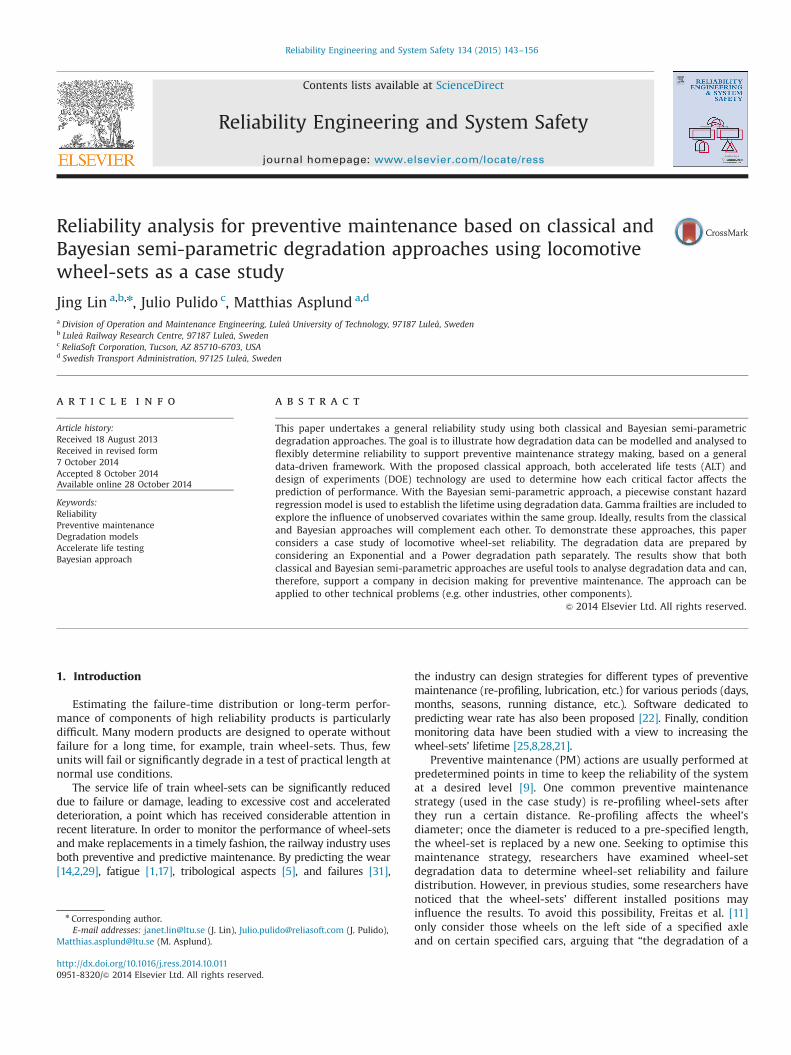
The data were collected by a Swedish company from November2010 to January 2012 (see Tables 5.1 and 5.2). They comprisedegradation data from two heavy haul cargo trains’ locomotives(denoted as Locomotive 1 and Locomotive 2). Accordingly, thereare two studied groups, andn¼ 2. For each locomotive, see Fig. 5.1,there are two bogies (Bogie I, Bogie II), and each bogie has sixwheel-sets, making a total of 12 wheels for each locomotive.

The diameter of a new locomotive wheel is 1250 mm. In thecompany’s current maintenance strategy, the wheel-set’s diameteris measured after running a certain distance; note that this is not adata-driven approach. If it is reduced to 1150 mm, the wheel-set isreplaced by a new one. Otherwise, it is re-profiled or other main-tenance strategies are implemented. Therefore, a threshold levelfor failure, denoted asl0, is defined as 100 mm (l0¼1250 mm�1150 mm). The wheel-set’s failure condition is assumed to be reachedif the diameter reaches l0. Tables 5.1 and 5.2 present the degradationdata for the wheel-sets of Locomotive 1 and Locomotive 2, separately.

5.2. Degradation path and lifetime data

From the dataset, we can obtain 3 to 5 measurements of thediameter of each wheel during its lifetime. By connecting thesemeasurements, we can determine a degradation trend. In theiranalyses of train wheel-sets, most studies [11,16] assume a lineardegradation path. In our study, considering both the results fromdegradation analysis in Weibullþþ and the type of physics offailure associated with wear and fatigue, we select Exponentialand Power degradation models. An Exponential model is describedby the following function (5.1) and the Power model by thesubsequent function (5.2):

Exponential : y¼ b� ea�x ð5:1Þ

Power : y¼ b� xa�c ð5:2Þwhereyrepresents the performance (here, it represents the dia-meters of the wheel-sets), xrepresents time (here, it represents therunning distance of the wheel-sets), and a,band c are modelparameters to be solved. Following the above discussion, we setl0¼y. The lifetimes for these wheels are now easily determinedand are shown in Table 5.3. As discussed by Lin et al. [16], somelifetime data can be viewed as right-censored (denoted by asteriskin Table 5.3).

5.3. Results and discussions from classical models

As shown in Figs. 5.2 and 5.3, the exponential function for thisset of data yields more conservative results and is in line with field

ReliaSoft DOE++ - www.ReliaSoft.com

Pareto Chart

Alpha = 0.1; Threshold = 1.7247Standardized Effect (T Value)

Term

0.000 30.0006.000 12.000 18.000 24.0001.725

AB

B:Bogie

A:Locomotive

Pareto Chart

Critical ValueSignificant

Julio PulidoReliasoft Corporation5/3/20139:50:45 AM

Fig. 5.4. Factors Pareto chart.

J. Lin et al. / Reliability Engineering and System Safety 134 (2015) 143–156150

observations when life data are compared at different stress levelsas previously defined. Fig. 5.3 shows reliability values for Loco-motive 2 and Bogie 2; both sides have 95% confidence level.

Using the exponential degradation model, we perform a twofactor full factorial DOE analysis and find that the locomotive,bogie and interaction are critical factors (see Fig. 5.4).

A review of the life stress relationship between the factorsindicates the locomotive is a higher contributor to the degradationof the system than the bogie (Figs. 5.5 and 5.6).

Based on the analysis, we can reach the following conclusions.Independent of the Degradation model, the locomotive is themore critical stressor, as shown in the data above. Failure modesobtained from the data are similar for the locomotive and thebogies. Of the two stress conditions, level 2 is the highest for thelocomotive and bogie, as shown in Fig. 5.6. Figs. 5.6 and 5.7 showthe reliability values at each operating distance. Fig. 5.7 shows thatLocomotive 2 has the highest degradation per distance travelled.

5.4. Results and discussions of Bayesian semi-parametric models

5.4.1. Parameter configurationIn this model, considering the wheels’ positions specified in

Section 5.1, the installed positions of the wheel-sets on a particularlocomotive are specified by the bogie number and are defined ascovariatesx. The covariates’ coefficients are represented by β. Morespecifically, x¼ 1 represents the wheels mounted in Bogie I, while

x¼ 2 represents the wheels mounted in Bogie II. β1 is thecoefficient, and β0 is defined as natural variability.

It is clear that a very smallkwill make the model nonparametric.However, if k is too small, estimates of the baseline hazard rate willbe unstable, and if kis too large, a poor model fit could result. Inour study, determining the degradation path requires us to make3 to 5 measurements for each locomotive wheel; in other words,the lifetime data are based on the data acquired at 3 to 5 differentinspections. Following the reasoning above, we divide the timeaxis into 6 sections piecewise. In our case study, no predicted life-time exceeds 360 000 km. Therefore, k¼6, and each interval isequal to 60 000 km. We get 6 intervals (0, 60 000], (60 000,120 00]… (300 000, 360 000].

For convenience, we letλk ¼ expðbkÞ, and vague prior distribu-tions are adopted as the following:

� Gamma frailty prior: ωi � Gaðκ�1; κ�1Þ� Normal prior distribution: bk �Nðbk�1; κÞ� Normal prior distribution: b1 �Nð0; κÞ� Gamma prior distribution: κ� Ga (0.0001, 0.0001)� Normal prior distribution: β0�N(0.0, 0.001)� Normal prior distribution: β1� N(0.0, 0.001)

At this point, the MCMC calculations are implemented with thesoftware WinBUGS [27]. A burn-in of 10 001 samples is used, withan additional 10 000 Gibbs samples.

Fig. 5.5. Life vs. stress.

J. Lin et al. / Reliability Engineering and System Safety 134 (2015) 143–156 151

5.4.2. Results from Bayesian semi-parametric modelFollowing the convergence diagnostics, we consider the follow-

ing posterior distribution summaries (Table 5.4): the parameters’posterior distribution mean, SD, MC error, and the 95% highestposterior distribution density (HPD) interval.

In Table 5.4, β140 means wheels mounted in the first bogie (asx¼ 1) have a shorter lifetime than those in the second (as x¼ 2).However, the influence could possibly be reduced as more data areobtained in the future, because the 95% HPD interval includes0 point. In addition, the small value of β1 (� 0.045) indicates that,in this case, heterogeneity among wheels installed in differentbogies exists but is not significant. Because κo0:5, heterogeneityamong the locomotives does exist but is not significant either.However, the frailty factors obviously exist. For instance, ω1o1suggests the predicted lifetimes for those wheels mounted on thefirst locomotive are longer than if the frailties are not considered;meanwhile, ω241 indicates the wheels mounted on the secondlocomotive have a shorter lifetime than if the frailties are notconsidered.

Baseline hazard rate statistics based on the above resultsðb1;…; b6Þ are shown in Table 5.5 and Fig. 5.8. At the fourthpiecewise interval, the wheels’ baseline hazard rate increasesdramatically (1481.78). It is interesting that at the fifth piecewiseinterval, it decreases (185.49) but increases again after the sixthpiecewise (22697.27).

By considering the random effects resulting from the naturalvariability (explained by covariates) and from the unobservedrandom effects within the same group (explained by frailties),we can determine other reliability characteristics of the lifetimedistribution. The statistics on reliability RðtÞ and cumulative hazard

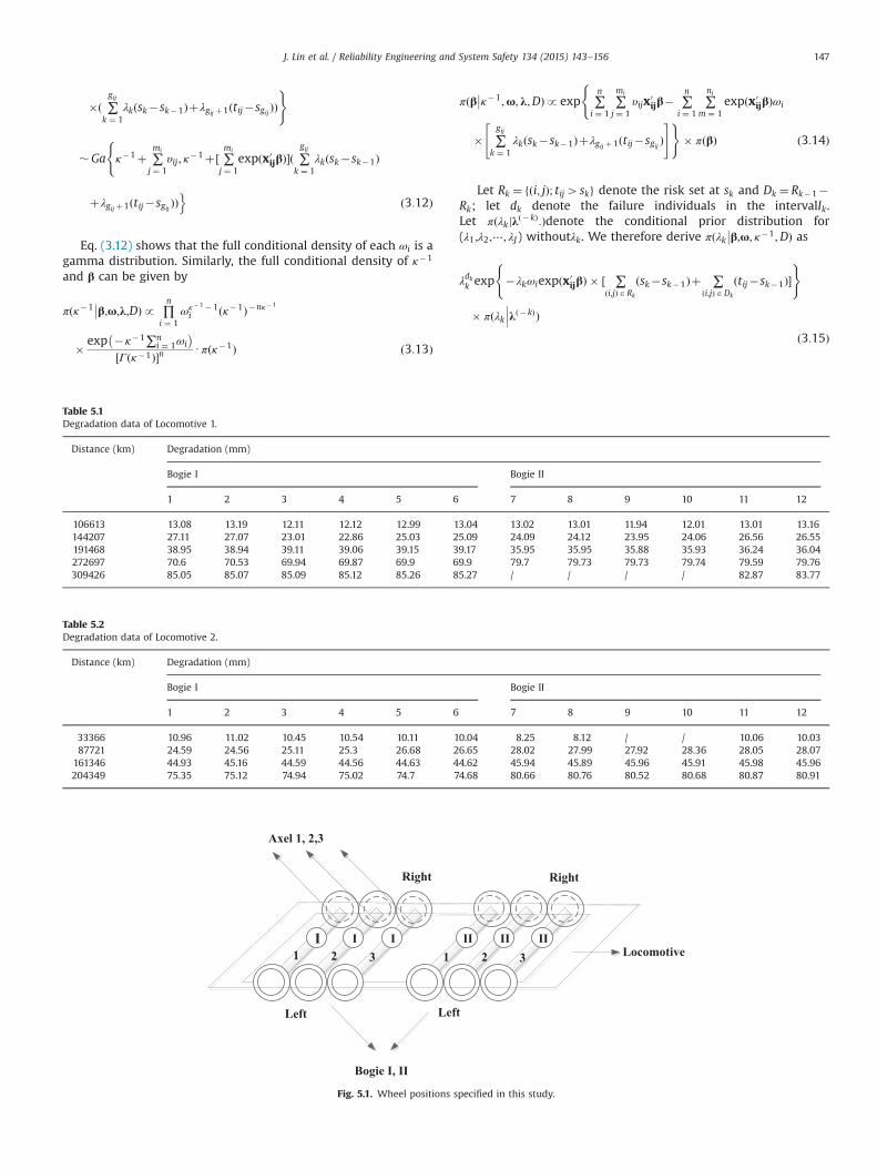
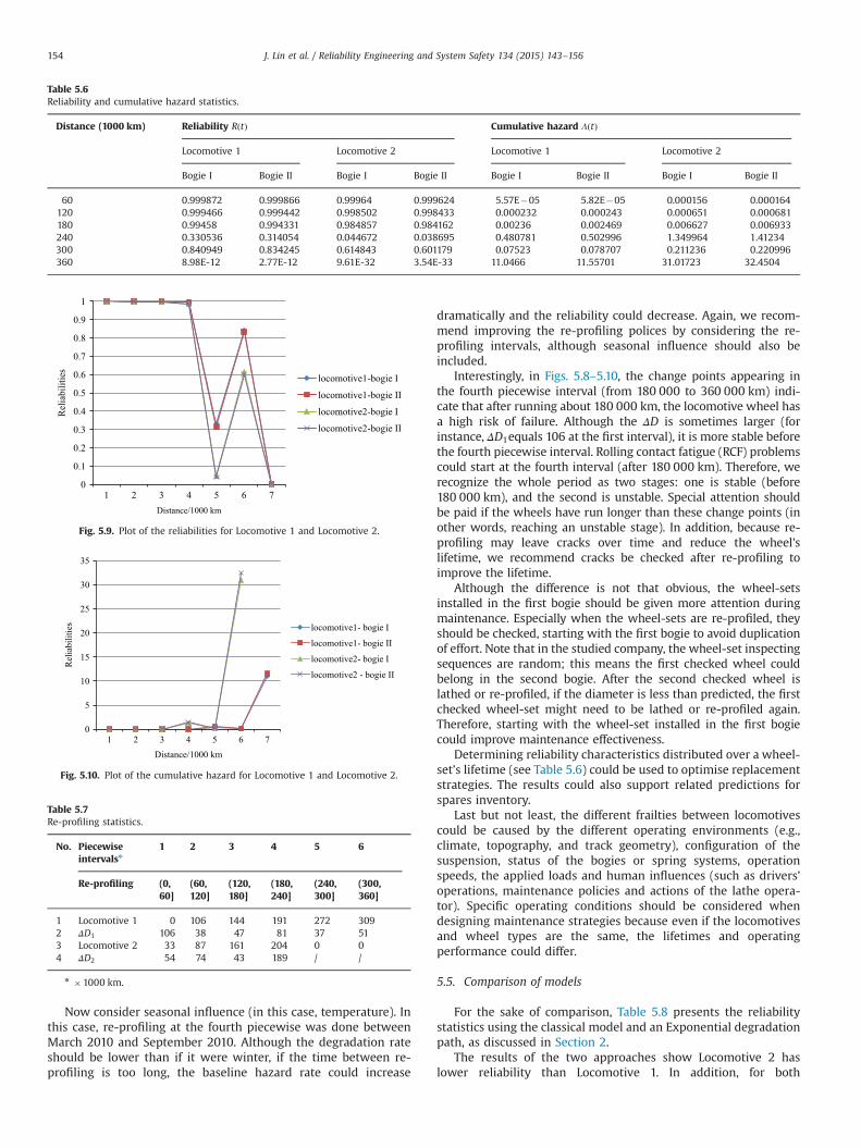
rate ΛðtÞ for the two wheels mounted in different bogies are listedin Table 5.6, Figs. 5.9 and 5.10.

For Locomotive 1 and Locomotive 2, Figs. 5.9 and 5.10 show theplots of reliability and cumulative hazard, respectively. It should bepointed out that both Figs. 5.9 and 5.10 show change points in thewheel-sets. For example, the reliability declines sharply at thefourth and the sixth piecewise interval. Meanwhile, after the fifthand the sixth piecewise interval, the cumulative hazard increasesdramatically.

5.4.3. Discussions from Bayesian semi-parametric modelThe above results (Section 5.4.2) can be applied to maintenance

optimisation, including wheel-set re-profiling optimisation, life-time prediction and replacement optimisation, and preventivemaintenance optimisation.

Before continuing, in Table 5.7, we list the re-profiling times(running distance/kilometres) for Locomotive 1 and Locomotive 2,separately (in rows 1 and 3). We can see the difference between re-profiling polices: for Locomotive 1, re-profiling is done, at most,5 times, whilst the wheels on Locomotive 2 are re-profiled, at most,4 times. For greater clarification, we list them under the k intervals.For instance, for Locomotive 1, the first re-profiling was performedat 106 000 km, placing it into the second piecewise interval. We candenote ΔDas the gap from the “current re-profiling” to the next onein each piecewise interval (rows 2 and 4). More specifically, forLocomotive 1, the first re-profiling is at 106 000 km, and the nextat 144 000 km, creating a gap of 38 000 km (¼144 000–106 000).For the last re-profiling, we use the boundary of 360 000 km asthe “next re-profiling”. By comparing ΔD, we can see the running

Locomotive2

Locomotive1

Bogie2 Bogie1

Fig. 5.6. Contour plot.

J. Lin et al. / Reliability Engineering and System Safety 134 (2015) 143–156152

distances of the wheels between profiling. If we do not consider thefirst interval's statistics (normally, the new wheel is treated asrunning in a good condition), the largest values appear at the fourth

interval for each locomotive, consistent with the findings fromFigs. 5.8 and 5.9. Therefore, the re-profiling time will influence thewheel-set degradation rate. If re-profiling is performed earlier than272 000 km for Locomotive 1, the degradation rate could bereduced, as could the baseline hazard rate. Meanwhile, the relia-bility in piecewise interval 4 could be increased. This conclusioncould also explain why at the fifth interval, the baseline hazard ratedecreases while the reliability increases. As discussed above, werecommend improving the re-profiling polices by considering there-profiling intervals.

Fig. 5.7. Reliability curves at each condition.

Table 5.4Posterior distribution summaries.

Parameter mean SD MC error 95% HPD interval

β0 �12.08 4.184 0.4019 (�22.17,�4.802)β1 0.04517 0.4889 0.02025 (�0.948,0.9669)κ 0.1857 0.1667 0.008398 (0.008616,0.6128)ω1 0.5246 0.2878 0.01401 (0.06489,1.064)ω2 1.473 0.5807 0.01596 (0.6917,2.948)b1 �0.3764 4.113 0.1619 (�8.316,5.933)b2 0.3571 4.95 0.2429 (�8.836,8.181)b3 2.272 4.61 0.3029 (�6.4,10.81)b4 7.301 4.106 0.3938 (0.2106,17.13)b5 5.223 4.225 0.3281 (�3.166,13.41)b6 10.03 3.993 0.3802 (2.72,19.3)

Table 5.5Baseline hazard rate statistics.

Piecewise intervals(�1000 km)

1 2 3 4 5 6

(0,60]

(60,120]

(120,180]

(180,240]

(240,300]

(300,360]

λk 0.069 1.43 9.7 1481.78 185.49 22697.27

Fig. 5.8. Plot of baseline hazard rate.

J. Lin et al. / Reliability Engineering and System Safety 134 (2015) 143–156 153

Now consider seasonal influence (in this case, temperature). Inthis case, re-profiling at the fourth piecewise was done betweenMarch 2010 and September 2010. Although the degradation rateshould be lower than if it were winter, if the time between re-profiling is too long, the baseline hazard rate could increase

dramatically and the reliability could decrease. Again, we recom-mend improving the re-profiling polices by considering the re-profiling intervals, although seasonal influence should also beincluded.

Interestingly, in Figs. 5.8–5.10, the change points appearing inthe fourth piecewise interval (from 180 000 to 360 000 km) indi-cate that after running about 180 000 km, the locomotive wheel hasa high risk of failure. Although the ΔD is sometimes larger (forinstance, ΔD1equals 106 at the first interval), it is more stable beforethe fourth piecewise interval. Rolling contact fatigue (RCF) problemscould start at the fourth interval (after 180 000 km). Therefore, werecognize the whole period as two stages: one is stable (before180 000 km), and the second is unstable. Special attention shouldbe paid if the wheels have run longer than these change points (inother words, reaching an unstable stage). In addition, because re-profiling may leave cracks over time and reduce the wheel'slifetime, we recommend cracks be checked after re-profiling toimprove the lifetime.

Although the difference is not that obvious, the wheel-setsinstalled in the first bogie should be given more attention duringmaintenance. Especially when the wheel-sets are re-profiled, theyshould be checked, starting with the first bogie to avoid duplicationof effort. Note that in the studied company, the wheel-set inspectingsequences are random; this means the first checked wheel couldbelong in the second bogie. After the second checked wheel islathed or re-profiled, if the diameter is less than predicted, the firstchecked wheel-set might need to be lathed or re-profiled again.Therefore, starting with the wheel-set installed in the first bogiecould improve maintenance effectiveness.

Determining reliability characteristics distributed over a wheel-set’s lifetime (see Table 5.6) could be used to optimise replacementstrategies. The results could also support related predictions forspares inventory.

Last but not least, the different frailties between locomotivescould be caused by the different operating environments (e.g.,climate, topography, and track geometry), configuration of thesuspension, status of the bogies or spring systems, operationspeeds, the applied loads and human influences (such as drivers’operations, maintenance policies and actions of the lathe opera-tor). Specific operating conditions should be considered whendesigning maintenance strategies because even if the locomotivesand wheel types are the same, the lifetimes and operatingperformance could differ.

5.5. Comparison of models

For the sake of comparison, Table 5.8 presents the reliabilitystatistics using the classical model and an Exponential degradationpath, as discussed in Section 2.

The results of the two approaches show Locomotive 2 haslower reliability than Locomotive 1. In addition, for both

Table 5.6Reliability and cumulative hazard statistics.

Distance (1000 km) Reliability RðtÞ Cumulative hazard ΛðtÞ

Locomotive 1 Locomotive 2 Locomotive 1 Locomotive 2

Bogie I Bogie II Bogie I Bogie II Bogie I Bogie II Bogie I Bogie II

60 0.999872 0.999866 0.99964 0.999624 5.57E�05 5.82E�05 0.000156 0.000164120 0.999466 0.999442 0.998502 0.998433 0.000232 0.000243 0.000651 0.000681180 0.99458 0.994331 0.984857 0.984162 0.00236 0.002469 0.006627 0.006933240 0.330536 0.314054 0.044672 0.038695 0.480781 0.502996 1.349964 1.41234300 0.840949 0.834245 0.614843 0.601179 0.07523 0.078707 0.211236 0.220996360 8.98E-12 2.77E-12 9.61E-32 3.54E-33 11.0466 11.55701 31.01723 32.4504

0

0.1

0.2

0.3

0.4

0.5

0.6

0.7

0.8

0.9

1

1 2 3 4 5 6 7

locomotive1-bogie I

locomotive1-bogie II

locomotive2-bogie I

locomotive2-bogie II

Rel

iabi

litie

s

Distance/1000 km

Fig. 5.9. Plot of the reliabilities for Locomotive 1 and Locomotive 2.

0

5

10

15

20

25

30

35

1 2 3 4 5 6 7

locomotive1- bogie I

locomotive1- bogie II

locomotive2- bogie I

locomotive2 - bogie II

Rel

iabi

litie

s

Distance/1000 km

Fig. 5.10. Plot of the cumulative hazard for Locomotive 1 and Locomotive 2.

Table 5.7Re-profiling statistics.

No. Piecewiseintervalsn

1 2 3 4 5 6

Re-profiling (0,60]

(60,120]

(120,180]

(180,240]

(240,300]

(300,360]

1 Locomotive 1 0 106 144 191 272 3092 ΔD1 106 38 47 81 37 513 Locomotive 2 33 87 161 204 0 04 ΔD2 54 74 43 189 / /

n �1000 km.

J. Lin et al. / Reliability Engineering and System Safety 134 (2015) 143–156154

Locomotive 1 and Locomotive 2, before the fourth piecewiseinterval, the reliability statistics from the classical approach havea higher value; after the fifth piecewise interval, the reliabilitystatistics from the Bayesian approach have a higher value.

In addition, considering the application process and resultsachieved by the different approaches in the case study, we can makethe following comparisons of classical and Bayesian approaches:

� First, the Bayesian semi-parametric degradation approachneeds less hypothesis than classical methods because thepiecewise constant hazard regression model is more flexible.

� Second, the dependence within subgroups can be consideredan unknown and unobservable risk factor of the gamma frailtymodel; fewer assumptions are required when implementingthe Bayesian approach.

� Third, the use of prior information from different sources willimprove the precision of the predictions, reflecting the super-iority of Bayesian approach.

� Fourth, with the Bayesian semi-parametric approach, change-points are more obvious and easily studied.

� Fifth, classical approaches are more reliable as the dataset islarge, but the Bayesian approach is dominant because thedataset is smaller. That being said, the dataset is large enough,so the choices made for PM strategies depend on preference oraccepted risk level.

� Sixth, the Bayesian approach is more complex and not as easilymanipulated by engineers; this complexity includes parameterconfiguration, MCMC implementation, etc.

� Seventh, the outputs from the classical approach are morefamiliar to applicators and, therefore, are more intuitive andmore easily interpreted and analysed.

In summary, using either approach has its advantages anddisadvantages. Following the above discussion, we recommendcomparing the results achieved by different approaches, acceptthem based on specified risk level when designing PM strategies,and use them to complement each other under specified condi-tions (for instance, a particular decision maker’s preference).

6. Conclusions

This paper proposes a reliability study based on a general data-driven framework using both classical and Bayesian semi-parametricdegradation approaches to illustrate how degradation data can bemodelled and analysed to flexibly determine reliability duringpreventive maintenance strategy making. The case study considersboth an Exponential and a Power degradation path for the wheel-setsof a locomotive and concludes the former is the better option. Using aclassical approach, it uses both accelerated life tests (ALT) and designof experiments (DOE) technology to determine how each critical

factor, i.e, locomotive and bogie, affects the prediction of perfor-mance. Within the Bayesian semi-parametric approach, the piece-wise constant hazard rate is used to establish the distribution of thewheel-set lifetime. The gamma shared frailtiesωiare used to explorethe influence of unobserved covariates within the same locomotive.By introducing covariatexi’s linear function x0

ijβ, the influence of thebogie in which a wheel is installed can be taken into account. TheMCMC technique is used to integrate high-dimensional probabilitydistributions to make inferences and predictions about model para-meters. The results from the classical and Bayesian semi-parametricapproaches can complement each other.

The results of the case study suggest the lifetime of wheel-setscan differ depending on where they are installed (in which bogiethey are mounted) on the locomotive. The gamma frailties helpwith exploring the unobserved covariates and, thus, they improvethe model's precision. We can determine wheel-set reliabilitycharacteristics, including the baseline hazard rate λðtÞ, reliabilityRðtÞ, and cumulative hazard rate ΛðtÞ. The results also indicate theexistence of change points. As Figs. 5.8–5.10 show, wheel-setreliability can be divided into two stages: stable and unstable at180 000 km. The results allow us to evaluate and optimise wheelreplacement and maintenance strategies (including the re-profiling interval, inspection interval, lubrication interval, depthand optimal sequence of re-profiling, and so on).

The proposed data-driven framework in this paper can beapplied to cargo train wheel-sets or to other technical problems(e.g. other industries, other components).

Acknowledgements

The authors would like to thank the editor and anonymousreferees for their constructive comments. The authors thank LuleåRailway Research Centre (Järnvägstekniskt Centrum, Sweden) andSwedish Transport Administration (Trafikverket) for initiatingthe research study and providing financial support (JVTC pro-jectnr:274). We also thank Richard House for his support in thereview and development of this paper. Finally, we thank ThomasNordmark, Ove Salmonsson and Hans-Erik Fredriksson at LKAB fortheir support and their discussions of the locomotive wheels.

References

[1] Bernasconi A, et al. An integrated approach to rolling contact sub-surfacefatigue assessment of railway wheels. J Wear 2005;258:973–80.

[2] Braghin F, et al. A mathematical model to predict railway wheel profileevolution due to wear. J Wear 2006;261:1253–64.

[3] Briano E., et.al. Design of experiment and Monte Carlo simulation as supportfor gas turbine power plant availabilty estimation. In: Proceedings of the 12thWSEAS international conference on AUTOMATIC CONTROL, MODELLING &SIMULATION. Conference proceedings. World Scientific and EngineeringAcademy and Society (WSEAS) Stevens Point, Wisconsin, USA. 2010: 223–230.

Table 5.8Reliability statistics using classical model.

Distance (1000 km) Reliability RðtÞ

Locomotive 1 Locomotive 2

Bogie I Bogie II Bogie I Bogie II

60 1.000000000000 1.000000000000 1.000000000000 1.000000000000120 1.000000000000 1.000000000000 1.000000000000 1.000000000000180 0.999999999500 0.999999999100 0.999949988500 0.999912782200240 0.999963596200 0.999936513100 0.032469287900 0.002535299700300 0.814489640600 0.699174645800 0.000000000000 0.000000000000360 0.000000000000 0.000000000000 0.000000000000 0.000000000000

J. Lin et al. / Reliability Engineering and System Safety 134 (2015) 143–156 155

[4] Clayton DG. A model for association in bivariate life tales and its application inepi-demiological studies of familial tendency in chronic disease incidence.Biometicka 1978;65:141–51.

[5] Clayton P. Tribological aspects of wheel–rail contact: a review of recentexperimental research. J Wear 1996;191:170–83.

[6] Craiu RV, Lee TCM. Model selection for the competing-risks model with andwithout masking. J Tech 2005;47(4):457–67.

[7] Demarqui FN, Loschi RH, Dey DK, Colosimo EA. A class of dynamic piecewiseexponential models with random time grid. J Stat Plann Inf 2012;142:728–42.

[8] Donato P, et al. Design and signal processing of a magnetic sensor array fortrain wheel detection. J Sens Actuators A 2006;132:516–25.

[9] Doostparast M, Kolahan F, Doostparast M. A reliability-based approach tooptimize preventive maintenance scheduling for coherent systems. J ReliabEng Syst Saf 2014;126:98–106.

[10] Douglas C. Montgomery design and analysis of experiments. 8th ed. Wiley;2012.

[11] Freitas MA, et al. Using degradation data to assess reliability: a case study ontrain wheel degradation. J Qual Reliab Eng Int 2009;25:607–29.

[12] Goulart A, Zhan W. A design of experiment (DOE) analysis of the performanceof uplink real-time traffic over a 3G network. In: IEEE international conferenceon wireless & mobile computing, networking & communication. Conferenceproceedings 2008. http://dx.doi.org/10.1109/WiMob.2008.110.

[13] Ibrahim JG, Chen MH, Sinha D. Bayesian survival analysis. New York: BerlinHeidelberg; 2001.

[14] Johansson A, Andersson C. Out-of-round railway wheels—a study of wheelpolygonalization through simulation of three-dimensional wheel–rail interac-tion and wear. J Vehicle Syst Dyn 2005;43(8):539–59.

[15] Levin MA, Kalal TT. Improving product reliability. John Wiley; 2003.[16] Lin J, Asplund M, Parida A. Reliability analysis for degradation of locomotive

wheels using parametric Bayesian approach. J Qual Reliab Eng Int2014;30:657–67.

[17] Liu YM, et al. Multiaxial fatigue reliability analysis of railroad wheels. J ReliabEng Syst Saf 2008;93:456–67.

[18] Meeker WQ, Escobar LA. Statistical methods for reliability data. Wiley; 1998.[19] Moghaddam KS, Usher JS. Sensitivity analysis and comparison of algorithms in

preventive maintenance and replacement scheduling optimization models. JComput Ind Eng 2011;61:64–75.

[20] Musharraf M, et al. A virtual experimental technique for data collection for aBayesian network approach to human reliability analysis. J Reliab Eng Syst Saf2014;132:1–8.

[21] Palo M. Condition-based maintenance for effective and efficient rolling stockcapacity assurance: a study on heavy haul transport in Sweden. Doctoralthesis. Luleå University of Technology, Sweden; 2014

[22] Pombo J, Ambrosio J, Pereira M. A railway wheel wear prediction tool based ona multibody software. J Theor Appl Mech 2010;48(3):751–70.

[23] ReliaSoft DOEþþ . Experiment design and analysis reference. ReliaSoft Cor-poration; 2008.

[24] Sahu SK, Dey DK, Aslanidou H, Sinha D. A Weibull regression model withgamma frailties for multivariate survival data. J Lifetime Data Anal1997;3:123–37.

[25] Skarlatos D, Karakasis K, Trochidis A. Railway wheel fault diagnosis using afuzzy-logic method. J Appl Acoust 2004;65:951–66.

[26] Soderholm P. A system view of the no fault found (NFF) phenomenon. J ReliabEng Syst Saf 2007;92:1–14.

[27] Spiegelhalter D., et al.. WinBUGS User Manual (Version 1.4). January; 2003.⟨http://www.mrc-bsu.cam.ac.uk/bugs⟩.

[28] Stratman B, Liu Y, Mahadevan S. Structural health monitoring of railroadwheels using wheel impact load detectors. J Fail Anal Prevent 2007;7(3):218–25.

[29] Tassini N, et al. A numerical model of twin disc test arrangement for theevaluation of railway wheel wear prediction methods. J Wear2010;268:660–7.

[30] Wienke A. Frailty models in survival analysis. PhD thesis; 2007.[31] Yang C, Letourneau S. Learning to predict train wheel failures. In: Conference

proceedings. The 11th ACM SIGKDD international conference on knowledgediscovery and data mining (KDD 2005). Chicago, Illinois, USA.

[32] Yuan T, et al. Bayesian analysis for accelerated life tests using a Dirichletprocess Weibull mixture model. J IEEE Trans Reliab 2014;63:58–67.

[33] Zhang X, Kang J, Jing T. Degradation modeling and maintenance decisionsbased on Bayesian belief networks. J IEEE Trans Reliab 2014;63:620–33.

Dr. Jing Lin is currently an Assistant Professor in the Division of Operation andMaintenance Engineering, at Luleå University of Technology (LTU), Sweden. Sheobtained her PhD degree in Management from Nanjing University of Science andTechnology (NJUST), China, in April 2008. After completing her doctorate, sheworked 3 years for SKF Co., Ltd as an Asset Management Consultant. Dr. Lin’sresearch interests primarily lie in RAMS and Asset Management. She has published50þ peer reviewed journal and conference papers.

Dr. Julio Pulido is a Sr. Director of Design for Reliability Engineering at ReliaSoftCorporation. His responsibility is to drive the capability development of Design forReliability for consulting clients. He holds a BS from the Federal University of Bahia,Brazil, an MS from the Federal University of Rio Grande do Sul, Brazil, a PhD fromthe Federal University of Rio de Janeiro, Brazil, PhD Research at Duke University andan MBA from Xavier University and a Certificate in Information TechnologyManagement from the University of Chicago. His specialty is in the area ofStructural Analysis, Design for vibration and Structural Reliability, and AcceleratedTesting Techniques. Dr. Pulido has 19þ years of experience in leading DesignAssurance Organizations. He has published over 50 works at different internationalsymposiums.

Matthias Asplund is a PhD student in the Division of Operation and MaintenanceEngineering, at Luleå University of Technology (LTU), Sweden, since 2011. Hisresearch area is RAMS with railway topics in focus. He has twelve years workingexperience from product development, lean production, maintenance and railwayengineering. He got his Master degree in Mechanical Engineering with focus onApplied Mechanics from Luleå Technical University. His last work before studies toPhD was Track Engineering for the Swedish Infrastructure Management.

J. Lin et al. / Reliability Engineering and System Safety 134 (2015) 143–156156