Embed Size (px)
Citation preview

Reliability Allocation and Assessment of Safety-Instrumented Systems
Jon Mikkel Haugen
Mechanical Engineering
Supervisor: Marvin Rausand, IPKCo-supervisor: Mary Ann Lundteigen, IPK
Department of Production and Quality Engineering
Submission date: December 2014
Norwegian University of Science and Technology


BNTNU2014.08.25 MARIKEDA
Faculty of Engineering Science and TechnologyDepartment of Production and Quality Engineedng
MASTER THESISAutumn 2014
ror stud. techn. Jon Mlkkel Haugen
Reiabifity allocation and assessment of safety-instrumented systems
(Pilltellghetsallokerlng og -vurdering av instrumenterte slkkerhetssystemer)
Reliability is an important property of any safety-instrumented system (515) and reliabilityconsiderations have to be integrated into a safety life cycle. Reliability requirements are specified ina safety requirement specification (SRS) and allocated to equipment and SIS subsystems based onthe potential risk. The general requirements to a 515 in the various phases of the safety life cycle aregiven in the generic standard IEC 61508 and in application-specific standards such as IEC 61511 forthe process industry and ifiC 62061 for machinery systems. A 515 is installed to perform one ormore safety-instrumented functions (SIPs) that should be activated when specific demands occur.When the demands occur more often than once per year, the SIP is said to be operating in high-demand mode, and when the demands occur more seldom, the SIP is operated in low-demand mode.The current master thesis is delimited to low-demand mode where the average probability of failureon demand (PFD) is used as reliability measure.
The objective of this master thesis is to study and evaluate main activities in the safety life cycle of alow-demand SIP.
As part of this master’s thesis, the candidate shall:1. Give a description of the safety life cycle and the activities required within selected phases.2. List the main elements of a typical SRS.3. Describe relevant approaches for the allocation of the safety integrity level (511.) of a defined
SIP and discuss pros and cons related to each approach.4. Select a suitable case study (in agreement with the supervisors) and (i) identify the relevant
demands and SIPs and (ii) determine the average PFD for each SIP.5. Discuss whether the case study system in item 4 is able to fulfil the other requirements in
IEC 61508 (e.g., architectural constraints)6. Discuss uncertainties related to the calculated average PFD.

Date Our reference
Master Thesis Spring 2014 for stud. techn. Jon Mikkel Haugen 2014.08.25 MAR/KEDA
Following agreement with the supervisor(s), [lie six tasks may he given different weights.
The assignment solution must be based on any standards and practical guidelines that already existand are recommended. This should be done in close cooperation with supervisors and any otherresponsibilities involved in the assignment. In addition it has to be an active interaction between allparties.
Within three weeks after [lie date of the task hand—out, a pre—study report shall be prepared. Thereport shall cover the following:
• An analysis of the work task’s content with specific emphasis of the areas where newknowledge has to he gained.
• A description of the work packages that shall be ierforrned. This description shall lead to aclear definition of the scope and extent of the total task to be performed.
• A time schedule for the project. The plan shall comprise a Gaiitt diagram with specificationof the individual work packages, their scheduled start and end dates and a specification ofproject milestones.
The pre—study report is a part of the total task reporting. It shall be included in the final report.Progress reports made during the project period shall also be included in the final report.
The report should be edited as a research report with a summary, table of contents, conclusion, list ofreference, list of literature etc. The text should be clear and concise, and include the necessaryreferences to figures, tables, and diagrams. It is also important that exact references are given to anyexternal source used in the text.
Equipment and software developed during the project is a part of the fulfilment of the task. Unlessoutside parties have exclusive property rights or the equipment is physically non—moveable, it shouldbe handed in along with the final report. Suitable documentation tbr the correct use of such materialis also required as part of the final report.
The student must cover travel expenses, telecommunication, and copying unless otherwise agreed.
IC the candidate encounters unibreseen difficulties in [lie work, and if these difficulties warrant areformation of the task, these problems should immediately be addressed to [lie Department.
The assignment text shall be enclosed and be placed immediately after the title page.

Date Our reference
Master Thesis Spring 2014 for stud. techn. Jon Mikkel Haugen 20 14.08.25 MAR/KEDA
Deadline: 1 2 January 2015
Two hound copies of the final report and one electronic (pdf-format) version are required accordingto the routines given in DAIM. Please see http://www.ntnu.edu/ivmaster-s-thesis-regulationsregarding master thesis regulations and practical information, inclusive how to use DAIM.
Responsible supervisor: Professor Marvin Rausand
E-mail: [email protected]
Co supervisor: Professor Mary Ann Lundteigen
E-mail: [email protected]
DEPARTMENT OF PRODUCTION
AND QUALITY ENGINEERING
Per SchjØlberg
Associate Professor/Head of Department
Marvin Rausand ,7
Responsible Supervisor

i
Preface
This master thesis is written during the fall semester of 2014 in Reliability, Availability, Maintain-
ability, and Safety (RAMS) at the Department of Production and Quality Engineering (IPK). This
is the final step of the five year master program in Mechanical Engineering at the Norwegian
University of Science and Technology (NTNU). The main motivation for choosing this topic was
to get extensive knowledge on safety-instrumented systems and relevant standards.
The thesis is mainly written for people with basic knowledge on reliability theory. However,
the standard IEC 61508 is introduced in a manner that hopefully makes the thesis enjoyable for
people with no prior knowledge on this topic.
Trondheim, 2012-12-22
Jon Mikkel Haugen


iii
Acknowledgment
I would first of all thank my supervisor Professor Marvin Rausand. I am extremely grateful for
his intelligent and reflective inputs. His guidance has been of great importance both for this
master thesis, but also on a personal level. I wish him all the best on his upcoming retirement.
Gratitude is also expressed to Professor Mary Ann Lundteigen for meaningful discussions and
valuable inputs on this master thesis.
Finally I would like to thank my friends, family and SO for supporting me and making the
master thesis period as painless as possible.
J.M.H


v
Summary and Conclusions
Safety-instrumented systems (SISs) are technical systems that are used to protect humans, the
environment, or assets from hazardous events. It is therefore important to ensure that these SISs
are reliable. IEC 61508 is an international standard that can be used to achieve this reliability for
SISs in all industries. It is also used to develop sector-specific standards such as IEC 61511 for
the process industry.
IEC 61508 frames the activities needed to ensure reliable SISs in a safety life cycle. Require-
ments for design, installation, operation, maintenance, and so on is given in the safety life cycle.
The methods and terminology presented in IEC 61508 is clarified in this thesis.
If the risk of a system is higher than what can be tolerated, the necessary risk reduction is
defined as the difference between actual risk and tolerable risk. The tolerable risk is achieved by
defining safety functions that reduce the risk. A safety-instrumented function (SIF) is a safety
function performed by a SIS. When a SIF is defined, an integrity requirement is set. The integrity
requirement is divided into four safety integrity levels (SILs). A SIL is a measure of how reliable
the SIF is. The reliability of a SIF determines its ability to prevent an undesired hazard. This way,
the integrity requirement can be translated into a reduction in risk for the system that the SIF
protects. The process of defining SIFs and determining their integrity requirements to achieve
tolerable risk is called SIL allocation. There are many ways to conduct SIL allocation. Some of
these methods are examined and discussed in this thesis.
An end-user of a SIS, for example an oil company, does usually not design their own SISs.
They analyze the system where a risk reduction is necessary and specify functional requirements
and integrity requirements for the SIS. These requirements are gathered in a safety requirements
specification. The content of the safety requirement specification is presented and discussed in
this thesis.
One of the application areas of a SIS is in subsea installations. To reduce the cost of flowlines
at the Kristin field, high integrity pressure protection systems are installed. The flowlines are
rated to a lower pressure than the pressure at the wellhead of the subsea well. To be able to
install these flowlines, a HIPPS is installed as an extra safety measure to block high pressure
flow to enter the flowline if the control system fails. The high integrity pressure protection have

vi
to achieve a SIL3 rating, which is the second strictest SIL rating.
To verify that the high integrity pressure protection at Kristin achieves a SIL3 rating, the av-
erage probability of failure on demand is calculated. This is a measure of the reliability of a SIS
that operates in a low-demand mode according to IEC 61508. Low demand mode means that
the SIF, on the average, is demanded less often than once per year. The calculations show that
the SIL3 requirement is met if all tests suggested in the case was implemented. It is also worth
mentioning that common cause failures represent a large proportion of unavailability of the SIF.
Common cause failures arise due to dependencies between some of the elements of the SIS. To
achieve a SIL3 rating, the SIS also has to fulfill requirements to robustness. These requirements
are called the architectural constraints. As shown in this thesis, the high integrity pressure pro-
tection system also fulfills the SIL3 according to the architectural constraints.
Assumptions and simplifications are made in the reliability assessments to enable the cal-
culation of reliability measures such as the average probability of failure on demand. This in-
troduces uncertainties in the calculations. The reliability data that is used will also constitute
uncertainty. It is discussed in the thesis that IEC 61508 maybe should introduce a framework for
uncertainty assessments as the uncertainty in cases with small margins might be decisive.

Contents
Preface . . . . . . . . . . . . . . . . . . . . . . . . . . . . . . . . . . . . . . . . . . . . . . . . i
Acknowledgment . . . . . . . . . . . . . . . . . . . . . . . . . . . . . . . . . . . . . . . . . . iii
Summary and Conclusions . . . . . . . . . . . . . . . . . . . . . . . . . . . . . . . . . . . . v
1 Introduction 1
1.1 Background . . . . . . . . . . . . . . . . . . . . . . . . . . . . . . . . . . . . . . . . . . 1
1.2 Objectives . . . . . . . . . . . . . . . . . . . . . . . . . . . . . . . . . . . . . . . . . . . 3
1.3 Limitations . . . . . . . . . . . . . . . . . . . . . . . . . . . . . . . . . . . . . . . . . . . 3
1.4 Structure of the Report . . . . . . . . . . . . . . . . . . . . . . . . . . . . . . . . . . . . 4
2 Safety-Instrumented Systems 5
2.1 Safety Barriers . . . . . . . . . . . . . . . . . . . . . . . . . . . . . . . . . . . . . . . . . 6
2.2 Safety-Instrumented Systems . . . . . . . . . . . . . . . . . . . . . . . . . . . . . . . . 7
2.3 IEC 61508 . . . . . . . . . . . . . . . . . . . . . . . . . . . . . . . . . . . . . . . . . . . . 12
2.4 Non Qualitative Requirements in IEC 61508 . . . . . . . . . . . . . . . . . . . . . . . 20
3 Reliability Allocation and SRS 27
3.1 Safety Requirement Allocation . . . . . . . . . . . . . . . . . . . . . . . . . . . . . . . 27
3.2 SIL Allocation Methods . . . . . . . . . . . . . . . . . . . . . . . . . . . . . . . . . . . 30
3.3 The Risk Graph Method . . . . . . . . . . . . . . . . . . . . . . . . . . . . . . . . . . . 31
3.4 LOPA . . . . . . . . . . . . . . . . . . . . . . . . . . . . . . . . . . . . . . . . . . . . . . 37
3.5 Minimum SIL Requirement . . . . . . . . . . . . . . . . . . . . . . . . . . . . . . . . . 44
3.6 Discussion on Reliability Allocation Methods . . . . . . . . . . . . . . . . . . . . . . 45
3.7 Safety Requirement Specification . . . . . . . . . . . . . . . . . . . . . . . . . . . . . 46
vii

CONTENTS 1
4 HIPPS case study 51
4.1 Case Description . . . . . . . . . . . . . . . . . . . . . . . . . . . . . . . . . . . . . . . 51
4.2 Calculating the PFD . . . . . . . . . . . . . . . . . . . . . . . . . . . . . . . . . . . . . 56
4.3 Uncertainty in PFD Calculation . . . . . . . . . . . . . . . . . . . . . . . . . . . . . . . 60
4.4 Evaluating Non-Integrity Requirements . . . . . . . . . . . . . . . . . . . . . . . . . . 63
5 Summary 67
5.1 Summary and Conclusions . . . . . . . . . . . . . . . . . . . . . . . . . . . . . . . . . 67
5.2 Recommendations for Further Work . . . . . . . . . . . . . . . . . . . . . . . . . . . . 69
A Acronyms 71
Bibliography 75
Curriculum Vitae 79

Chapter 1
Introduction
1.1 Background
Electrical/electronic/programmable electronic (E/E/PE) safety-related systems, herein referred
to as SISs, are technical systems designed to protect humans, the environment, and assets from
harm. Failures of SISs may lead to unwanted consequences. Ensuring the reliability of these
systems is therefore essential to safety. This is done by conducting a reliability assessment of
the SIS. The international standard IEC 61508, Functional safety of E/E/PE safety-related systems,
provides a proven methodology to achieve reliable SISs. This standard is generic, to ensure
applicability to all SISs. In addition, it is used to develop sector-specific standards such as IEC
61511 for the process industry and IEC 62061 for machinery systems.
IEC 61508 introduces the safety life cycle (SLC), which provides a step-by-step method con-
taining requirements for design, installation, operation, maintenance, and commissioning of
the SIS. The standard provides a risk-based approach to determine the requirements of the SIS.
When an end-user acquires a SIS, these requirements are gathered in a safety requirement spec-
ification (SRS). The SRS contains a detailed description on which functions the SIS is intended
to provide, and how well it shall perform them. The supplier have to demonstrate that these
requirements are met. This is done by quantifying the reliability performance and demonstrate
compliance to the given architectural constraints. The architectural constraints are introduced
in IEC 61508 to ensure a robust architecture of the SIS.
1

CHAPTER 1. INTRODUCTION 2
IEC 61508 presents two distinct reliability integrity measures for a SIS. For a SIS operating in
low-demand mode the average probability of failure on demand (PFDavg) is applied. For a SIS
operating in high-demand or continuous mode of operation the average frequency of dangerous
failures per hour (PFH) is used. The demand rates for these modes are less than, and more often
than, once a year, respectively.
The reliability measures for the SIS are based on an identified need for a risk reduction within
a delimited system, which is called the equipment under control (EUC). This risk reduction is
the difference between tolerable risk and actual risk. SIFs, and their corresponding integrity re-
quirements, are defined to introduce a risk reduction sufficient to achieve acceptable risk. This
process is called the allocation process in IEC 61508. The allocation process can be performed by
several different methods. The risk graph method and the layers of protection analysis (LOPA)
are two of the methods that are suggested for this purpose in IEC 61508 and IEC 61511.
The risk graph method has been extensively debated (e.g., Baybutt, 2007; Baybutt, 2014;
Nait-Said et al., 2009; Salis, 2011). All of these studies point to weaknesses of the method, mostly
due to the fundamental methodology of the risk graph and risk matrices. Baybutt (2007) sug-
gests an improved risk graph method to overcome this challenge. The LOPA method was in-
troduced by CCPS (1993) for the process industry. This is a systematic approach that can be
used integrated with a hazard and operability study (HAZOP). It can be used to determine the
risk reduction of existing, or suggested, protection layers, such as SISs. Many variations of the
method have been developed (e.g., Rausand, 2011; CCPS, 2001; IEC 61511, 2003; BP, 2006; Sum-
mers, 2003). These methods enable a risk-based determination of reliability targets for SIFs.
The method in NOG-070 (2004) contains prescriptive requirements for typical SIFs under cer-
tain prerequisites. This method also complies with the requirements in IEC 61508. So which
method is to be preferred?
SISs have a wide application area. The oil- and gas industry handles hydrocarbons, which
constitute a high risk environment. To reduce this risk, several SISs are installed at offshore in-
stallations. Also certain subsea installations apply SISs to increase safety. A high integrity pres-
sure protection system (HIPPS), is an example of such a SIS. A case study of the HIPPSs installed
at the Kristin field outside Trondheim forms the basis for an examination of the functional and
integrity requirements. As the integrity requirements are determined through the use of relia-
CHAPTER 1. INTRODUCTION 3
bility models and probabilistic models, possible sources of uncertainty are also examined.
1.2 Objectives
The main objectives of this master thesis are:
1. Clarify basic concepts and terminology in IEC 61508. Give a description of the safety life
cycle and the activities required within selected phases.
2. Describe relevant approaches for the allocation of the SIL of a defined SIF and discuss
pros and cons related to each approach.
3. List the main elements of a typical SRS.
4. Carry out a case study of a subsea HIPPS,
• identify the relevant demands and SIFs
• determine the average PFD for each SIF
5. Discuss whether the HIPPS case study is able to fulfill the other requirements in IEC 61508
(e.g., architectural constraints).
6. Discuss uncertainties related to the calculated average PFD for the HIPPS case study.
Remark: In agreement with the supervisors, the objectives of this master thesis are changed.
The objectives stated above applies.
1.3 Limitations
This thesis mainly applies terminology and methodology from IEC 61508. To delimit the thesis,
software requirements (IEC 61508, 2010, Part 3), and human and organizational factors are not
considered. For calculations in Chapter 4, the PDS-method (SINTEF, 2013b) and formulas from
Rausand (2014) are applied. Other methods are briefly mentioned. As the HIPPS case study is a
low-demand system, other demand modes are not thoroughly discussed in this thesis.

CHAPTER 1. INTRODUCTION 4
1.4 Structure of the Report
The rest of the report is structured as follows. Chapter 2 gives an introduction to SIS and the
basic concepts and terminology from IEC 61508. Chapter 3 describes the reliability allocation
process with emphasis on risk graph method, LOPA, and minimum SIL approach. SRS is also
briefly presented. The HIPPS case study is presented in Chapter 4, and the PFDavg is calculated
and discussed. This chapter also includes a discussion on fulfillment of the non-integrity re-
quirements of the HIPPS case, as well as a discussion on uncertainties related to the calculated
PFDavg. Chapter 5 summarizes and concludes this master thesis, and gives some recommenda-
tions for further work. Acronyms are presented in Annex A.

Chapter 2
Safety-Instrumented Systems
Safety is one of the most, if not the most, important system characteristics. But what does the
word safety mean? A brief introduction to safety and safety barriers is provided in this chapter
to illustrate the main goal of a SIS; to improve safety. Further a thorough introduction to SIS and
the basic concepts and methodology in IEC 61508 is given.
One of the most commonly used definitions of the term safety is presented in MIL-STD-882D
(2000):
Z Safety (1): Freedom from those conditions that can cause death, injury, occupational illness,
damage to or loss of equipment or property, or damage to the environment.
According to this definition, safety is only achieved if the probability of any assets being
harmed, for example personal injury, is equal to zero. This definition can be problematic, as
there are no practical way to remove all hazards in a system. Rausand (2011) suggests a more
practical definition:
Z Safety (2): A state where the risk has been reduced to a level that is as low as reasonable
practicable (ALARP) and where the remaining risk is generally accepted. 1
1ALARP can be defined as: "A level of risk that is not intolerable and cannot be reduced further without theexpenditure of costs that are grossly disproportionate to the benefit gained". For further reading see e.g. Rausand(2011)
5

CHAPTER 2. SAFETY-INSTRUMENTED SYSTEMS 6
This definition is used in this thesis as it allows for the practical definition of a safe system
through the acceptability of risk.
2.1 Safety Barriers
When engineering a system, you need to be able to consider whether or not the system is safe.
Relating this to the definition of safety, we have to consider if the risk that is introduced is gen-
erally accepted or not. For a company engineering a system, the term generally accepted can
be misleading. If you are designing a process facility, there are many standards, laws and reg-
ulations that govern what risk level that is considered acceptable. These documents have been
developed in order to ensure a common practice between companies and serve as the govern-
ment’s way to safeguard its population. This way, these documents reflect a risk level that is
generally accepted.
Initial to the design process it is necessary to define the risk acceptance criteria. Risk accep-
tance criteria are defined by NS 5814 (2008) as:
Z Risk acceptance criteria: Criteria used as a basis for decision about acceptable risk.
The risk acceptance criteria can be regarded as the minimum level of safety we require the
system to provide. The preliminary system design will often result in a potential risk higher than
the risk acceptance criteria. In these cases, we have to install one or more barriers, or more
precise, safety barriers. A safety barrier can be defined as (Sklet, 2006, p.505):
Z Safety barrier: A physical and/or nonphysical means planned to prevent, control, or miti-
gate undesired events or accidents.
Barrier Classification
Barriers can be classified in a number of ways. A main distinction that is useful when analyzing
barrier systems is proactive and reactive barriers. They can be defined as (Rausand, 2011, p.366):

CHAPTER 2. SAFETY-INSTRUMENTED SYSTEMS 7
Barrier function
Barrier system
Passive Active
PhysicalHuman and/or
operationalTechnical
Human and/or operational
Safety instrumented system (SIS)
Other technology safety-related system
External risk reduction facilities
Figure 2.1: Classification of barriers (reproduced from Sklet, 2006).
Z Proactive barrier: A barrier that is installed to prevent or reduce the probability of a haz-
ardous event. A proactive barrier is also called a frequency-reducing barrier.
Z Reactive barrier: A barrier that is installed to avoid, or reduce the consequences of a haz-
ardous event. A reactive barrier is also called a consequence-reducing barrier.
A more comprehensive classification is proposed by Sklet (2006), and is shown in Figure 2.1.
This classification distinguishes technical and human and/or operational barriers. It also di-
vides the active technical barriers into SISs, other technology safety-related systems, and exter-
nal risk reduction facilities. This thesis focuses on SIS and how the reliability of SIS affects the
overall system safety.
2.2 Safety-Instrumented Systems
A SIS is a common type of safety barrier. As shown in Figure 2.1, a SIS can be categorized as
an active technical barrier. A SIS consists of three main subsystems; input element(s), logic

CHAPTER 2. SAFETY-INSTRUMENTED SYSTEMS 8
Logicsolver
Input elements
Final elements
Figure 2.2: The main elements of a SIS (reproduced from Rausand, 2011).
solver(s), and final element(s). An illustration is shown in Figure 2.2. A SIS can either function
as a proactive or a reactive barrier. The SIS is installed in an EUC. An EUC is the specific delim-
ited hazardous system that is evaluated, such as machinery, process plant, and transportation.
Usually the EUC also has a control system. The objective of the EUC control system is to mon-
itor and control the EUC to ensure desirable operation (IEC 61508, 2010). A SIS is designed
to be activated upon one or more specific hazardous process demands. A process demand is a
measurable deviation from normal operation. An EUC may produce several of these hazardous
process demands.
Functional Safety
A safety barrier is designed to introduce one or more safety functions. The purpose of a safety
function is to bring he EUC to a safe state. A safe state can be defined as "a state of the EUC
where safety is achieved" IEC 61508. Specifically, a SIS performs one or more SIFs upon specific
process demand in the EUC. It is important to separate the terms; SIS, SIF, and safety function. A
SIS denotes the physical system. The SIF is the function performed by the SIS to increase safety.
A SIF is a subset of safety functions.
Failure- and Failure Mode Classification
In order to analyze the reliability of a SIS, it is important to understand the ways a SIS can fail
and how this will impact the EUC risk. Generically, a SIS has two distinct failure modes:

CHAPTER 2. SAFETY-INSTRUMENTED SYSTEMS 9
1. A process demand occurs in the EUC, but the SIS is unable to perform the corresponding
SIF, denoted fail-to-function (FTF) failure mode in this thesis.
2. The SIS performs a SIF although the corresponding process demand has not occurred in
the EUC, denoted spurious trip (ST) failure mode in this thesis.
Not all failure modes are critical for performing the SIF. Hence, it can be useful to classify the
failure modes in this respect. The following classification is proposed in IEC 61508:
(a) Dangerous failure (D). The SIS is unable to perform the required SIF upon demand from
the EUC. Dangerous failures can be divided into:
• Dangerous undetected (DU). A dangerous failure has occurred, but is only revealed
through testing of the SIS or if a SIF process demand occurs in the EUC.
• Dangerous detected (DD). A dangerous failure has occurred but is immediately de-
tected through, for example, diagnostic testing.
(b) Safe failure (S). The SIS-failure is not considered dangerous. Safe failures can be divided
into:
• Safe undetected (SU). A safe failure has occurred and is not detected.
• Safe detected (SD). A safe failure has occurred and is immediately detected.
In order to increase the reliability of the SIF, it is necessary to analyze the failure mechanisms
that lead to these failure modes. IEC 61508 distinguishes between random hardware failures and
systematic failures:
Z Random hardware failure: Failure occurring at a random time, which results from one or
more of the possible degradation mechanisms in the hardware.
Z Systematic failure: Failure related in a deterministic way to a certain cause, which can only
be eliminated by a modification of the design or of the manufacturing process, operational pro-
cedures, documentation or other relevant factors.

CHAPTER 2. SAFETY-INSTRUMENTED SYSTEMS 10
Examples of systematic failures can be human error in design of both hardware and software.
If these failures occur, it is likely that they will not reoccur after an improvement is carried out.
Systematic failures is discussed more thoroughly in Section 2.4. Examples of random hardware
failures are mechanical stresses and wear. It is also important to note the difference between a
failure and a fault. A failure is a time dependent event. After a failure occurs, and the ability to
perform the required function is terminated, the item will usually be in a failed state. This failed
state is called a fault. Hence, a failure is an event while a fault is a condition.
Common Cause Failures
Common cause failures (CCFs) is a specific type of failure resulting from one or more events
that causes concurrent failure of two or more channels in a multiple channel system, leading to
a fault state of the system IEC 61508. These failures origin due to both intrinsic and extrinsic de-
pendencies between channels. CCFs are often caused by systematic failures and can be avoided
by using similar defense mechanisms that are presented in Section 2.4.
As the nature of CCFs are different than independent failures IEC 61508 requires that the
CCFs are treated separately. The process of calculating the common cause failures are shortly
presented in Section 2.3.
SIS Configuration
As mentioned a SIS comprises of at least three subsystems. These subsystems may comprise
of one or more voted groups of channels. A channel consist of one or more elements that solely
perform a function which is a part of the SIF. An example of a channel is a solenoid valve and a
downhole safety valve (DHSV) designed to close an oil well on demand. The solenoid receives
an electronic signal to open. When the solenoid opens, it allows for hydraulic fluid to close the
DHSV and hence conclude the SIF.
A voted group consists of two or more similar channels that perform the same function. It is
important to note that the term should only be used if all the channels are identical. An example
of a voted group is three level transmitters (LTs) channels.
If a group consist of n channels, it can be voted in several ways. The term voting describes
how many of the channels that has to function, denoted k, in order to perform the required

CHAPTER 2. SAFETY-INSTRUMENTED SYSTEMS 11
Level transmitter
1oo3 votingLevel
transmitter
Level transmitter
V
Figure 2.3: 1oo3 voted structure of LTs.
function of the group. This is referred to as a k-out-of-n voted structure. An example of this is
a 1oo3 structure of LTs, meaning that at least one of three LTs have to function in order for the
group to perform its function. An illustration of this voted group is shown in Figure 2.3.
Testing
SISs are usually off-line as long as no process deviation occurs. Therefore, they have to be tested
to reveal potential faults. According to Rausand (2014) these tests are designed to confirm cor-
rect performance and confirm that the SIS responds as intended to specific faulty conditions.
There are three categories of tests in the operational phase of a SIS (Rausand, 2014):
• Proof testing: Planned periodic test designed to reveal DU fault of each channel. The
proof test should also detect which of the elements that have failed and caused the oc-
currence of a DU failure. The proof test assumes that the SIS performs as-good-as-new
after testing is completed. Not all DU faults can be detected by a proof test. If this is the
case, the proof test coverage (PTC) should be defined. A perfect proof test assumes that the
PTC=100%. An imperfect proof test assumes that the PTC<100%.
• Partial testing: Planned test designed to reveal one or more specific DU faults of a chan-
nel. The idea behind the partial test is that some DU faults can be revealed without dis-
turbing the EUC. Partial stroke testing (PST) is a common example of partial testing. A
valve is partially closed, and then returned to initial position. This does not fully block
production and several DU faults are potentially revealed. The partial proof test coverage
(PPTC) can be used to denote the coverage of this test type.
CHAPTER 2. SAFETY-INSTRUMENTED SYSTEMS 12
Concept1
Overall scope definition2
Hazard and risk analysis3
Overall safety requirements
4
Overall safety requirements allocation
5
E/E/PE system safety requirements specification
9
E/E/PE safety-related systems
10Specification and realisationRealisation
(see E/E/PE system safety lifecycle)
Overall installation and commissioning
12
Overall safety validation13
Overall operation, maintenance and repair
14
Decommissioning or disposal
16
Overall planning
Overall operation and maintenance planning
6Overall safety validation planning
7
Overall installation and commissioning planning
8
Overall modification and retrofit
15
Other risk reduction methods
11
Back to appropriate overall safety lifecycle
phase
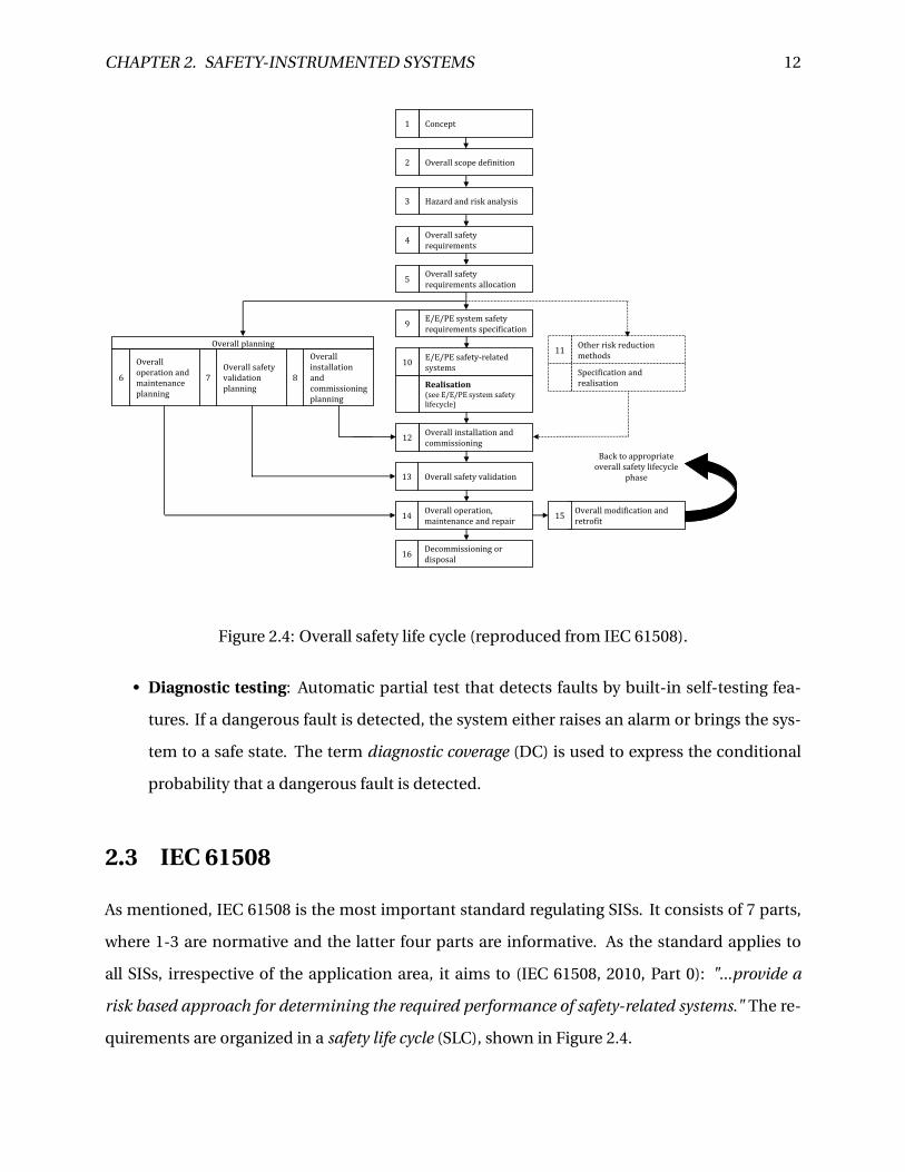
Figure 2.4: Overall safety life cycle (reproduced from IEC 61508).
• Diagnostic testing: Automatic partial test that detects faults by built-in self-testing fea-
tures. If a dangerous fault is detected, the system either raises an alarm or brings the sys-
tem to a safe state. The term diagnostic coverage (DC) is used to express the conditional
probability that a dangerous fault is detected.
2.3 IEC 61508
As mentioned, IEC 61508 is the most important standard regulating SISs. It consists of 7 parts,
where 1-3 are normative and the latter four parts are informative. As the standard applies to
all SISs, irrespective of the application area, it aims to (IEC 61508, 2010, Part 0): "...provide a
risk based approach for determining the required performance of safety-related systems." The re-
quirements are organized in a safety life cycle (SLC), shown in Figure 2.4.

CHAPTER 2. SAFETY-INSTRUMENTED SYSTEMS 13
Safety Life Cycle
As the SLC frames the activities to meet the requirements in the standard, the different phases
and the corresponding objectives are introduced. The phases that are discussed in more detail
in later chapters contains cross references. The objectives of the phases are to:
1. Concept
• Develop a sufficient level of understanding of the EUC in order to enable the next life
cycle phases to be carried out satisfactorily.
2. Overall scope definition
• Develop and delimit the boundaries for the EUC and its control system.
• Specify the scope of the hazard and risk analysis.
3. Hazard and risk analysis
• Carry out a hazard analysis to determine hazards and hazardous events (HE) relating
to both the EUC and its control system. All modes of operation have to be consid-
ered.
• Carry out a risk analysis to determine event sequences and establish the EUC risk.
4. Overall safety requirements
• Develop the specification for the overall safety requirements.
• Determine the required safety functions and corresponding safety integrity require-
ments for any SIS and other risk reduction measures.
5. Overall safety requirements allocation
• Allocate the safety functions and safety integrity requirements to the designated SIS
and/or other risk reduction measures.
• Allocate a safety integrity level to each SIF carried out by a SIS. The process of alloca-
tion is further discussed in Chapter 3.

CHAPTER 2. SAFETY-INSTRUMENTED SYSTEMS 14
6. Overall operation and maintenance planning
• Develop a plan for operation and maintenance for the SIS. This aims to ensure the
functional safety during operation and maintenance.
7. Overall safety validation planning
• Develop a plan for the overall safety validation of SISs based on the information and
results from phase five.
8. Overall installation and commissioning planning
• Delvelop a plan for the installation of SISs that minimizes the risk of introducing
systematic failures and ensures the required functional safety.
• Develop a plan for the commissioning of SISs ensuring the required functional safety.
9. E/E/PE system safety requirements specification
• Develop a safety requirements specification (SRS) for each SIS containing one or
more SIFs. Both functional requirements and safety integrity requiremens are de-
fined.
• The content of an SRS is further presented in Section 3.7.
10. Realization: E/E/PE safety-related systems
• Design and create a SIS conforming to the SRS developed in phase nine.
11. Other risk reduction methods
• Design and create other risk reduction measures in order to meet the overall safety
requirements developed in phase four.
12. Overall installation and commissioning
• Install and commission the SIS according to the plan developed in phase eight.
13. Overall safety validation

CHAPTER 2. SAFETY-INSTRUMENTED SYSTEMS 15
• Validate that the SIS meets the requirements in the SRS according to the plan devel-
oped in phase seven.
14. Overall operation, maintenance and repair
• Ensure that the functional safety of the SIS is maintained throughout operation and
maintenance.
• This is achieved by ensuring that technical requirements necessary for operation
and maintenance of the SIS i provided to those responsible for future operation and
maintenance.
15. Overall modification and retrofit
• Define a procedure that ensures functional safety of the SIS both during and after the
modification and retrofit phase.
• Necessary to ensure a systematic approach to modification of the SISs and hinder
the introduction of new risk to the system.
16. Decommissioning or disposal
• Define necessary procedures to ensure functional safety of the SIS during and acter
decommissioning or disposal of the SIS.
As seen from the presentation from the SLC, the main focus is to ensure functional safety of
the SIS throughout its lifetime. There are two main requirements for achieving this functional
safety; functional requirements and safety integrity requirements.
Safety Integrity Requirements
Safety integrity is defined as (IEC 61508): "probability of an E/E/PE safety related system satis-
factorily performing the specified safety functions under all the stated conditions within a stated
period of time". The goal of this requirement is to determine how well the SIS is required to per-
form the SIF(s). IEC 61508 defines four SILs as a way to measure the safety integrity of a SIS,

CHAPTER 2. SAFETY-INSTRUMENTED SYSTEMS 16
Table 2.1: Safety integrity levels (adapted from IEC 61508).SIL Low-demand mode PFDavg High-demand mode (PFH)
4 ≥ 10−5to < 10−4 ≥ 10−9to < 10−8
3 ≥ 10−4to < 10−3 ≥ 10−8to < 10−7
2 ≥ 10−3to < 10−2 ≥ 10−7to < 10−6
1 ≥ 10−2to < 10−1 ≥ 10−6to < 10−5
ranging from SIL 1 to SIL 4. SIL 1 is the least reliable and SIL 4 the most reliable. The different
levels and respective reliability target measures are presented in Table 2.1.
The reliability measurement used for SIL depends on the mode of operation of the SIS per-
forming the various SIFs. IEC 61508 distinguishes between three different operational modes:
• Low-demand mode: The safety function is performed on demand. The frequency of de-
mand is less than once per year.
• High-demand mode: The safety function is performed on demand. The frequency of de-
mand is higher than once a year.
• Continuous mode: The safety function is performed continuously so the EUC is retained
in a safe state.
As seen from the definitions there are two demand modes and one continuous mode. Ta-
ble 2.1 on the other hand only present two different reliability target measures. This is because
IEC 61508 for most purposes separates between low- and high-demand. The reliability measure
is therefore the same for high-demand mode and continuous mode, the probability of a danger-
ous failure per hour (PFH). Low-demand mode systems use the average probability of failure on
demand (PFDavg).
Reliability Measure for Low-Demand
When a DU failure has occurred in a SIS element, it is not able to perform the required SIF upon
demand. The unavailability of a SIF due to this DU failure is called the probability of failure on
demand (PFD) when it is operating in low-demand. To apply the simplified formulas introduced
by Rausand and Høyland (2004), the following assumptions are made:

CHAPTER 2. SAFETY-INSTRUMENTED SYSTEMS 17
• The SIS elements have a constant DU failure rate, λDU
• Proof tests designed to reveal DU failures are perfect, such that all failures are revealed
• When SIS elements are repaired, they are considered "as good as new"
• The time for testing and possible repair is considered to be negligible
• Only considers random hardware failures
Given these assumptions, the PFD at time t of a SIS put into function at time t = 0 is given by
(Rausand, 2011):
PFD(t ) = Pr (TDU ≤ t ) = 1−e−λDUt (2.1)
As seen from the formula the limit of PFD when t →∞ is one, hence it is needed to include
proof testing at time τ to decrease the unavailability of the SIF. Given all the assumptions above
all test intervals have the same stochastic properties (0,τ], (τ,2τ], . . . (Rausand, 2011).
Due to the stochastic properties of (2.1) and practical purposes IEC 61508 recommends a
simplification when calculating the PFD using the PFDavg. This can be derived accordingly:
PFDavg = 1
τ
∫ τ
0(1−eλDUt )d t = 1
λDUτ(1−eλDUτ) (2.2)
By introducing the Maclaruins series for e−λDUτ and assuming a small λDUτ (Rausand and
Høyland, 2004) suggests the following approximation for a 1oo1 system:
PFD(1oo1)avg ≈ λDUτ
2(2.3)
For simplified formulas for other configurations see Rausand and Høyland (2004). IEC 61508
deviates from the simplified formulas at it includes the unavailability caused by the mean repair

CHAPTER 2. SAFETY-INSTRUMENTED SYSTEMS 18
time (MRT) after a DU failure, and the mean time to repair (MTTR) when a DD failure is revealed.
According to Rausand (2014) neglecting these unavailability contributors will in most cases give
an adequate result. NOG-070 suggests a different approach. The PFDavg in NOG-070 consists
of the unavailability of DU failures caused by random hardware failures and systematic failures.
The concepts for calculating PFDavg in IEC 61508 and NOG-070 are not further discussed in this
chapter as the simplified formulas will be applied in Chapter 4.
Reliability Measure for High-Demand
PFH is the reliability measure for a DU-failure in a SIS-element operating in high-demand mode
or continuous mode. The main distinction from PFDavg is that PFH is a measure of the frequency
of failure and not an unavailability measure. According to IEC 61508 the PFH is the average
unconditional failure intensity. To better understand this measure it useful to begin with the
definition of frequency of failures denoted w(t ) and defined as (Rausand, 2014):
w(t ) = d
d tE [N (t )] (2.4)
where E [N (t )] represents the mean number of failures at time t. By utilizing the definition
of the derivative and assuming 4t to be small we find that:
w(t ) ≈ E [N (t +4t )−N (t )]
4t
Meaning that w(t ) represents the frequency of failures in the time interval (t , t +4t ). For
very small 4t ) the number of failures of a SIF in this time interval will be either 0 or 1. Utilizing
the definition of the mean value gives us the following result:
w(t ) = Pr[Failure in(t , t +4t )]
4t
The frequency of failure at time t is often called the rate of occurrence of failures (ROCOF)

CHAPTER 2. SAFETY-INSTRUMENTED SYSTEMS 19
(Rausand, 2014).
The PFH as a concept is the same as the ROCOF. The time dependent PFH(t ) is given by:
PHF(t ) = wD(t ) (2.5)
where wD(t ) represents the ROCOF at time t with respect to dangerous failures. In IEC 61508
the requirement is that the average PFH is used as the reliability measure for high-demand and
continuous operating SIFs. For the time interval (0,T) the average PFH is defined as:
PHF = 1
T
∫ T
0wD(t )d t (2.6)
As this thesis focuses on low-demand SISs, the subject of PFH will not be discussed in more
detail. For further reading on this topic see e.g., Rausand (2014).
Calculating CCFs
The beta-factor model is a common method used to incorporate CCFs into reliability models
(Rausand, 2014). The main idea in this model is to split the failure rate, λ, into an individual
failure rate,λ(i ), and a failure rate that affects all the items in a voted group,λ(c). The relationship
between these parameters is given by λ=λ(i )+λ(c). β is introduced to describe the ratio of CCFs
(Rausand, 2014):
β= λ(c)
λ(2.7)
A further development of this method was introduced by Hokstad and Corneliussen (2004)
and is called the multiple beta-factor model. This method is used in the PDS method (SINTEF,
2013b). The main addition to the method was the possibility to distinguish the CCF contribution
according to the configuration of the SIS. The rate of CCFs for a koon system is given as (SINTEF,

CHAPTER 2. SAFETY-INSTRUMENTED SYSTEMS 20
2013b):
β(koon) =β ·Ckoon ; (k < n) (2.8)
The correction factor Ckoon is an estimate based on expert judgment. A procedure to de-
velop this correction factor is outlined in Appendix B of SINTEF (2013b). The multiple beta-
factor model is used in the calculations i Chapter 4. The PFDavg of a koon structure is given as
(Rausand, 2014):
PFDavg = PFD(i )DU +PFD(CCF)
DU (2.9)
A more thorough description of the beta-factor model and the multiple beta-factor model
is not provided as this task is too comprehensive given the objectives of this thesis. For more
information on CCFs see e.g., Rausand (2014).
2.4 Non Qualitative Requirements in IEC 61508
Architectural Constraints
In addition to the quantifiable reliability measures IEC 61508, contains prescriptive require-
ments for the robustness of the structure. These requirements are called architectural con-
straints and are introduced to limit the hardware architecture of the SIS on the basis of PFH
and PFDavg alone. According to IEC 61508 there are two ways to comply with these require-
ments, called route 1H and 2H. However it does not suggest which route to choose for specific
systems, but this may be indicated in sector-specific standards.
Route 1H
Route 1H uses the concept of safe failure fraction (SFF) and hardware fault tolerance (HFT) to de-
termine the the limits of the achievable SIL. In order to determine the architectural constraints

CHAPTER 2. SAFETY-INSTRUMENTED SYSTEMS 21
Lundteigen (2009) suggests a four-step procedure presented in Figure 2.5.
Step 1: Assess and classify subsystem elements
An element of the subsystem are classified with respect to the complexity and operational expe-
rience. This is a measure meant to address the uncertainty of the elements behavior. IEC 61508
classifies the elements as type A or type B. Type A elements are characterized by well defined
failure modes, where the behavior of the element is completely determined, and the field expe-
rience data is sufficient to document the reliability performance. If an element cannot meet one
or more of these requirements, it is considered a type B element.
Step 2: Calculate the SFF
The SFF is a parameter that reflects the probability of an element or a subsystem to fail to a safe
state. Given constant failure rates, the SFF is defined as (IEC 61508, 2010):
SFF =∑λS +∑
λDD∑λS +∑
λDD +∑λDU
(2.10)
It is important to note that it is the sum of failures of each category, meaning that all failure
modes have to be categorized and summed up before calculating the SFF. The SFF is calculated
for each subsystem. As seen from the definition the dangerous detected failures are consid-
ered as safe as the SFF assumes immediate follow-up and repair. In case of redundancy in the
subsystem, the SFF must be defined for each channel if the channels comprise of dissimilar
components.
Table 2.2: Hardware fault tolerance table (adapted from IEC 61508).SFF/HFT
Type A Type B0 1 2 0 1 2
<60% SIL1 SIL2 SIL3 - SIL1 SIL260-90% SIL2 SIL3 SIL4 SIL1 SIL2 SIL390-99% SIL3 SIL4 SIL4 SIL2 SIL3 SIL4
>99% SIL4 SIL4 SIL4 SIL3 SIL4 SIL4

CHAPTER 2. SAFETY-INSTRUMENTED SYSTEMS 22
Step 3: Determine the achievable SIL for the subsystem
The first task in this step is to determine the HFT. A HFT of N implies that if N+1 faults occur
the ability of the subsystem to perform the required function is terminated. This factor is deter-
mined by assessing the voting of the subsystem. As an example, a 1oo3 voted group can tolerate
up to 2 channels in a fault state. Hence, the HFT of a 1oo3 voted group is 2. When the HFT
has been determined the achievable SIL is found for each subsystem. The achievable SIL level
is presented in Table 2.2. As seen from this table, the achievable SIL for a subsystem consisting
of type A elements is higher than in if the same subsystem consisted of type B elements. This
is because using type B elements introduces a higher uncertainty as the lack of knowledge of
failure modes and the impact of operational conditions is limited. This rule may be regarded as
a "rule of thumb" on how to handle uncertainty. There is little doubt that the requirements is
based on good engineering intentions though the improvement in reliability performance can
be questioned.
Step 4: Determine the achievable SIL of the SIF
As the SIL for each subsystem has been determined, the final step is to develop the achievable
SIL for each SIF. Depending on the configuration of subsystems, IEC 61508 proposes a set of
merging rules:
• If two subsystems are connected in series, the maximum achievable SIL for the SIF is equal
to the SIL of the subsystem having the lowest SIL.
• If two subsystems are connected in parallel, the maximum achievable SIL for the SIF is
equal to the SIL of the subsystem having the highest SIL plus N, where N represents the
HFT of a koon system.
Route 2H
The main idea behind this method is that we have increased confidence in systems that have
been used for a long period of time. This leads to a small probability of systematic failures and
better knowledge on random hardware failures. To be able to utilize route 2H certain criterion
have to be met. The available reliability data has to be based on field feedback for elements used

CHAPTER 2. SAFETY-INSTRUMENTED SYSTEMS 23
Per SIF
Per subsystem
Per subsystem
Per subsystem
Assess and classify subsystem elements
Calculate SFF for each element
Determine HFT for each element
Determine the achievable SIL of subsystem
1
2 3
Determine the achievable SIL of SIF
4
Figure 2.5: Four-step procedure to determine the architectural constraints (inspired fromLundteigen, 2009).
in a similar application and environment, the data collection is handled according to interna-
tional standards and the amount of data have to be sufficient. The goal of these requirements is
to present the uncertainty of reliability target measures such as the PFDavg. In order to comply
with the requirement it is necessary to run simulations to verify that the calculated target failure
measures are improved to a confidence greater than 90%.
The method determines the HFT for each subsystem in a SIS that performs a SIF of a spec-
ified SIL. The rules of this method are given in Table 2.3. It is important to note a discrepancy
that may imply to a type A element. If the required HFT is larger than one and the introduction
of a redundant element implies additional failures that ultimately decrease the overall safety of
the EUC, a safer alternative architecture with a lower HFT may be implemented.
Table 2.3: Route 2H determining factors.Operational mode SIL of SIF Minimum HFT
Low-demand
SIL1 0SIL2 0SIL3 1SIL4 2
High-demand andcontinuous mode
SIL1 0SIL2 1SIL3 1SIL4 2

CHAPTER 2. SAFETY-INSTRUMENTED SYSTEMS 24
Critique of Architectural Constraints
The architectural constraints have been met with some skepticism. IEC 61508 claims that the
architectural constraints is necessary to address the complexity of an element and/or subsys-
tems and to ensure "robustness". Both end users and system integrators have questioned why
the standard introduces prescriptive requirements as it is stated in the objectives of the standard
that: "IEC 61508 aims to provide a risk-based approach for determining the required performance
of safety-related systems". This is considered to be somewhat of a contradiction as the risk-based
approach bases on the belief that the reliability of a system may be estimate and used as a basis
for decision-makers.
The main critique of the architectural constraints have been the use of SFF as a parameter
and the foundation of the SFF-HFT-SIL relationship (e.g., Lundteigen (2009); Signoret (2007);
Lundteigen and Rausand (2006)). As the SFF has a direct impact on the need for redundancy
in the SIS it is crucial that the definition of this parameter is solid. In the earlier versions of
IEC 61508, the calculation of SFF considered all safe failures. This meant that it was possible
to achieve a higher SFF if more non-dangerous safe failures were introduced. However, this
potential flaw was fixed in the latest version of IEC 61508 as non-critical failures as a whole
was left out of the calculation of λS. The PDS-method (SINTEF, 2013b) also utilizes the same
definition. This alteration silenced most of the critique of the SFF parameter.
Systematic Safety Integrity
As the reliability target measures and the architectural constraints only considers random hard-
ware failures, IEC 61508 contains requirements for avoidance and control of systematic failures.
Both the definition of random hardware failure and systematic failures have been debated. Rau-
sand (2014) questions what the term "degradation mechanisms" covers in relation to random
hardware failures. In contrast to the PDS-method (SINTEF, 2013b) which restricts the random
hardware failures to aging failures that occur due to external stresses within the design enve-
lope, Rausand (2014) also includes some human errors and excessive eternal stresses such as
lightening. The main argument for this definition is that the data from reliability databases, like
OREDA, can be efficiently utilized. As these databases do not separate on failure mechanisms

CHAPTER 2. SAFETY-INSTRUMENTED SYSTEMS 25
the use of other definitions of random hardware failures will increase the data uncertainty. Es-
pecially in borderline cases where there are uncertainty whether a SIF can be accepted as a SIL
X the applied definition of hardware failures should be discussed in the reliability assessment.
This topic shows that differences on how to define random hardware failures also impacts
the effect of systematic failures, as all failures should be treated in reliability assessments accord-
ing to IEC 61508. The definition suggested in IEC 61508 emphasize that the systematic failures
can be eliminated through modification in design or the manufacturing process, or through
operational procedures and documentation. Therefore the standard provides a rather compre-
hensive list of techniques and measures to avoid the introduction of systematic failures in all
SLC phases. IEC 61508 introduces a measure called systematic capability to describe the safety
integrity of the SIS with regards to systematic failures:
Z Systematic capability: Measure (expressed on a scale of SC 1 to SC 4) of the confidence that
the systematic safety integrity of an element meets the requirements of the specified SIL, in re-
spect of the specified element safety function, when the element is applied in accordance with
the instructions specified in the compliant item safety manual for the element.
The standard describes three routes to achieve systematic capability; route 1S, route 2S, and
route 3S. Route 1S demands compliance with the requirements for avoidance and control of sys-
tematic faults. Route 2S demands that the equipment can be documented as "proven in use".2
Route 3S applies only for pre-existing reused software elements and demands thorough docu-
mentation to prove the systematic capability in the new application.
The PDS-method argues that systematic failures should be quantified. This is due to the un-
availability of the safety function a systematic failure will cause. They introduce a probability of
systematic failure (PSF). This is not a requirement in IEC 61508, but both the PDS-method SIN-
TEF (2013b) and NOG-070 (2004) recommends to apply the PSF as a reliability target measure.
This topic is not further discussed as it goes beyond the scope of this thesis.
2Requirements for proven in use elements are given in section 7.4.10 in IEC 61508 (2010, part 2)


Chapter 3
Reliability Allocation and SRS
The allocation of risk reduction measures and safety functions is an important activity in the SLC
shown in Figure 2.4. After development of the required safety functions in step four, the main
task in step five is to allocate these safety functions to various safety barriers. This includes
allocation of the SILs and the associated SIFs. This chapter aims to present some of the most
relevant approaches for SIL allocation. The pros and cons of the methods are also discussed.
The development of an SRS is a key step to be able to realize the required risk reduction
introduced by a given SIF. The requirements to an SRS in IEC 61508 are listed. A brief discussion
on the topic is also included.
3.1 Safety Requirement Allocation
The process of allocating the overall safety requirements is shown in Figure 3.1. In order to en-
sure a successful allocation it is important to understand what the required input should con-
tain, and how it is determined. Therefore, a brief introduction of the general input required is
given. Depending on the nature of the allocation method presented in this chapter, the required
input will vary.
Input to SIL Allocation
When the EUC and its control system are defined, it is common to conduct a hazard identifica-
tion. The goal of this process is to determine the relevant hazardous events for the EUC and its
27

CHAPTER 3. RELIABILITY ALLOCATION AND SRS 28
Allocation of each safety function and its
associated safety integrity requirement
Other risk reduction measures #1
Other risk reduction measures #2E/E/PE safety-
related system #2
E/E/PE safety-related system #1
E/E/PE safety-related system #1
E/E/PE safety-related system #2
E/E/PE safety-related system #1
E/E/PE safety-related system #2
Development of SRS for SIS #1
Development of SRS for SIS #2
Method of specifying the safety integrity
requirements
Necessary risk reduction
Necessary risk reduction
Safety Integrity Levels (SILs)
Figure 3.1: Allocation of overall safety requirements (reproduced from IEC 61508).
control system, including fault conditions and foreseeable misuse. Examples of relevant meth-
ods are (HAZOP), hazard identification (HAZID), failure modes, effects, and criticality analysis
(FMECA), structured what-if technique (SWIFT), and more. For further information on these
methods see, for example, Rausand (2011).
The results from the hazard identification are then used to determine the event sequences,
the corresponding occurrence frequencies, and finally the total EUC risk. Examples of methods
that can be applied is fault tree analysis (FTA) and event tree analysis (ETA). For further study of
these methods see, for example, Rausand (2011). The end result of the risk analysis is a quantifi-
cation of risk presented through one or more risk metrics. Two examples are (Rausand, 2014):
Z Fatal accident rate (FAR): The expected number of fatalities in a defined population per 100
million hours of exposure.
Z Individual risk per annum (IRPA): The probability that an individual will be killed due to a
specific hazard or by performing a certain activity during one year’s exposure.

CHAPTER 3. RELIABILITY ALLOCATION AND SRS 29
These risk metrics form the basis for the allocation process. As mentioned in Chapter 2 prior
to designing systems, it is common practice to define a risk acceptance criterion. The safety life
cycle process in IEC 61508 uses the term tolerable risk, based on the same concept of societal
acceptance of risk as risk acceptance criteria:
Z Tolerable risk: Risk which is accepted in a given context based on the current values of soci-
ety.
The measure of tolerable risk will vary dependent on regulations, company policies, societal
expectation, and so on. Whether or not the risk is tolerable can also depend on how much a
reduction in risk will cost. A common approach to determine the tolerable risk is the ALARP
principle as mentioned in Chapter 2. The method divides risk into three levels. The unaccept-
able region where the risk cannot be accepted independent of cost. The broadly accepted region
where the risk is acceptable and no risk reduction is required. The ALARP-region is the region
where risk reducing measures should be introduced as long as the risk reduction is not imprac-
ticable or the cost is grossly disproportionate to the improvement gained. For further reading
see, for example, Rausand (2011).
When the EUC risk and the tolerable risk have been determined, the necessary risk reduction
can be calculated. This is found by subtracting the tolerable risk from the EUC risk. After all the
safety functions have been introduced in the EUC, the remaining risk is called the residual risk.
An overview of the general concept of this risk reduction process for low-demand systems is
presented in Figure 3.2. The overall concept is also similar for high-demand systems, but IEC
61508 operates with other critical factors than for the low-demand systems. The critical factor
for high-demand systems is dangerous failure rate, whereas it is PFD for low-demand systems.
The residual risk is also denoted residual hazard rate as high-demand systems are based on
frequencies, not demands.

CHAPTER 3. RELIABILITY ALLOCATION AND SRS 30
EUC risk
Tolerable risk
Residual risk
Increasing risk
Necessary risk reduction
Actual risk reduction
Partial risk covered by other risk reduction
measures #2
Partial risk covered by safety instrumented
systems
Partial risk covered by other risk reduction
measures #1
Risk reduction achieved by all the safety instrumented systemsand other risk reduction measures
Figure 3.2: Risk reduction - general concept and terms (reproduced from IEC 61508).
3.2 SIL Allocation Methods
The first step of the SIL allocation is to allocate the overall safety function to various safety bar-
riers. These safety barriers can be SISs or other risk reduction methods. A safety function can
be carried out by one or more SISs and/or other risk reduction methods. IEC 61508 does not
provide any generic method for allocation of overall safety functions, but it stresses the need for
skilled personnel in this process. It also mentions specifically that it, depending on the EUC,
may be critical to include skills and resources from operation and maintenance and the operat-
ing environment.
The next step of the allocation process is to determine the required SIL for all SIFs performed
by the SISs. IEC 61508 suggests five different methods for this purpose:
• The ALARP method
• Quantitative method of SIL determination
• The risk graph method
• Layers of protection analysis (LOPA)
• Hazardous event severity matrix

CHAPTER 3. RELIABILITY ALLOCATION AND SRS 31
The methods are both qualitative, quantitative and semi-qualitative to ensure that meth-
ods for any application area are presented. This chapter describes the risk graph method and
the LOPA method. NOG-070 does not contain any risk-based approaches to SIL allocation. In-
stead, it presents another approach called minimum SIL requirement. This approach is briefly
presented as it can give an indication of how SIL allocation is done in practice.
3.3 The Risk Graph Method
The risk graph method is based on knowledge on risk factors associated with the EUC and the
EUC control system to determine the required SIL of the SIFs. The method is suggested for SIL
allocation for machinery (IEC 62061, 2005, Annex A), the process industry (IEC 61511, 2003, Part
3), and has also been used in the chemical industry (Salis, 2011). It allows for both qualitative
and quantitative assessments of the EUC risk. A number of parameters that describe the nature
of the HE are described. These are described without considering any introduced SIFs. Ac-
cording to IEC 61508, the requirements for the parameters are that they allow for a meaningful
gradation of the risk and that they contain the key risk assessment factors of the EUC. In IEC
61508, these risk parameters are chosen to be adequately generic to deal with the wide range
of application areas. The standard provides a simplified procedure and a general scheme pre-
sented in Figure 3.3. This generic example uses four parameters to describe the nature of the
HE (IEC 61508, 2010, Annex E, part 5):
C denotes the consequence of the HE. The consequence can be related to personal injury,
the environment, and so on.
F denotes the frequency of, and exposure time in, the hazardous zone.
P denotes the possibility of failing to avoid the HE.
W denotes the probability of the HE.
As seen in Figure 3.3, the number of possible scenarios is eighteen. The combination of
C, F, and P represents the frequency of a HE, while C represents the consequence of a HE. All
scenarios are then assigned a SIL requirement dependent on the total risk. In this example, the

CHAPTER 3. RELIABILITY ALLOCATION AND SRS 32
a
1
2
3
4
b
---
a
1
2
3
4
---
---
a
1
2
3
𝑾𝟑 𝑾𝟐 𝑾𝟏
a = No special safety requirement
--- = No special safety requirement
b = A single SIS is not sufficient
1,2,3,4 = Safety integrity level
CA
CB
CC
CA
FA
FB
FAFB
FA
FB
PA
PB
PAPB
PB
PB
PA
PA
X1
X2
X3
X4
X5
X6
Starting point for risk reduction
estimation
Figure 3.3: Risk graph - general scheme (reproduced from IEC 61508).
Initiating event
End event #1
End event #2
End event #3= Accident scenario
Figure 3.4: Accident scenario.
SIL requirement ranges from not required, through SIL 1-4, to not sufficient. The risk graph
method can be conducted with respect to safety, environment, economic impact and so on.
However, it is important to note that only one of these properties can be evaluated at once.
Risk Graph Procedure Considerations
The risk graph procedure can easily be misinterpreted. A function block presenting the input
and output to the procedure is shown i Figure 3.5. As the procedure is based on a decision
logic tree, such as the example in Figure 3.3, the application area is rather limited. The start-

CHAPTER 3. RELIABILITY ALLOCATION AND SRS 33
Determine SIL by risk graph
End event
Demand rate 1
SIL-requirement
Demand rate 2
Calibration Tolerable risk
Figure 3.5: Risk graph functional block.
ing point of a risk graph procedure is an end event. An end event is the final condition in an
accident scenario that starts with an initiating event. An illustration of these terms are shown
in Figure 3.4. The reason why the end event is the starting point is that it is the first time in an
accident scenario where the consequence can be determined. As the first parameter in the risk
graph decision tree is a classification of consequence, this has to be known. This is a limiting
factor of the risk graph as every end event have to be considered individually. The number of
end events are usually a lot bigger than the number of initiating events, making the procedure
very time consuming.
Qualitative vs. Quantitative Risk Graph
IEC 61511 presents two variations of the risk graph. The traditional risk graph is a qualitative
method. The parameters presented are divided into levels of qualitative measures. The quanti-
tative version is called the calibrated risk graph. The parameters in this version are divided into
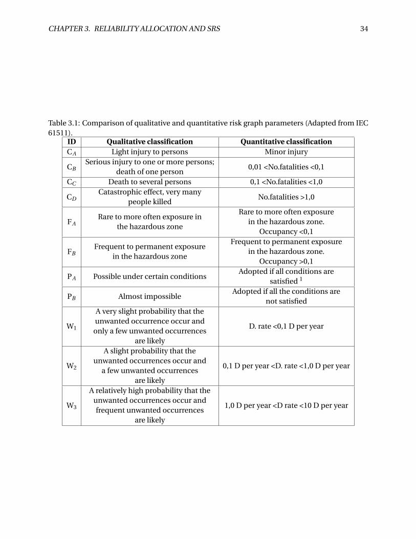
levels of quantitative measures. Table 3.1 shows a suggested classification of parameters for the
risk graph and the calibrated risk graph with respect to safety.
The process of assigning numerical values to the parameters in the calibrated risk graph is
called calibration. This can be a time-consuming process as all parameters are divided into
numerical values according to the EUC under consideration and the mentioned requirements.
After the calibration of the graph is completed, the SIL allocation is performed for each SIF.
The allocation is determined by a decision-making process for each parameter, resulting in a
SIL requirement for the SIF.
CHAPTER 3. RELIABILITY ALLOCATION AND SRS 34
Table 3.1: Comparison of qualitative and quantitative risk graph parameters (Adapted from IEC61511).
ID Qualitative classification Quantitative classificationCA Light injury to persons Minor injury
CBSerious injury to one or more persons;
death of one person0,01 <No.fatalities <0,1
CC Death to several persons 0,1 <No.fatalities <1,0
CDCatastrophic effect, very many
people killedNo.fatalities >1,0
FARare to more often exposure in
the hazardous zone
Rare to more often exposurein the hazardous zone.
Occupancy <0,1
FBFrequent to permanent exposure
in the hazardous zone
Frequent to permanent exposurein the hazardous zone.
Occupancy >0,1
PA Possible under certain conditionsAdopted if all conditions are
satisfied 1
PB Almost impossibleAdopted if all the conditions are
not satisfied
W1
A very slight probability that theunwanted occurrence occur and
only a few unwanted occurrencesare likely
D. rate <0,1 D per year
W2
A slight probability that theunwanted occurrences occur and
a few unwanted occurrencesare likely
0,1 D per year <D. rate <1,0 D per year
W3
A relatively high probability that theunwanted occurrences occur andfrequent unwanted occurrences
are likely
1,0 D per year <D rate <10 D per year

CHAPTER 3. RELIABILITY ALLOCATION AND SRS 35
Improved Risk Graph Method
Baybutt has through several publications criticized the risk graph method (see e.g., (2007); (2012);
(2014)). He introduces an improved risk graph to overcome some of his critiques to the tradi-
tional risk graph (Baybutt, 2007). The most important significant alteration is that the improved
risk graph focuses on scenario risk, not the consequences. The method follows the flow of a
hazardous scenario. It is also designed as a decision tree but the parameters, and the number of
levels for each parameter, are changed. The parameters are presented in Table 3.2.
Table 3.2: Improved risk graph parameters (based on Baybutt, 2007).Parameter Description LevelsInitiators [I] Initiating cause frequency 6Enablers [E] Enabling events/conditions and other modifiers 2Safeguards [S] Safeguard failure probability 3Consequences [C] Consequences of the hazardous event or sceanario 5
Initiators are events that cause a failure of an equipment, such as a leakage of a valve. The
initiator frequency is divided into six levels. Enablers are conditions that have to be fulfilled in
order for a specific scenario to develop, but is not a direct cause of an HE. The enabler parameter
is divided into two levels as "present" or "not-present." The safeguard parameter assesses the
preventive counter-measures to the initiators. Divided into three levels based on the presence
of category 1 and 2 safeguards. Whether a safeguard is category 1 or 2, is based on its reliability
performance. The consequence parameter is to a large extent the same as in the traditional risk
graph.
An advantage of the improved risk graph is that it is directly linked to analyses that are al-
ready conducted, such as a HAZOP and risk analysis. This is due to the chosen parameters and
the decision-making process. It also facilitates application of more refined methods such as
LOPAs or quantitative risk analyses (QRAs).
Strengths and Weaknesses
As mentioned, the risk graph have been extensively debated. There are some clear strengths
with this approach. It can be conducted both qualitatively and quantitatively using the same
methodology. It is rather easy to understand and apply for simple systems. However, there are

CHAPTER 3. RELIABILITY ALLOCATION AND SRS 36
numerous weaknesses and limitations in the application of the risk graph. According to Smith
and Simpson (2011) the risk graph is only suitable for low-demand systems. This is because of
the rule-based algorithm that leads to a request for a demand rate.
A well known weakness is the determination, and calibration of the parameters. There is
generally a lack of knowledge on how to use the parameters and the uncertainty this leads to
(e.g., Smith and Simpson, 2011; Nait-Said et al., 2009; Baybutt, 2007; Salis, 2011). To exemplify,
if the calculated consequence of an HE is 0,08 expected deaths per event the consequences are
in the range [10−2, 10−1]. This will result in an optimistic evaluation. If this also is the case for
the other parameters, the end result will be an underestimation of the SIL. An overestimation
of the SIL can also occur this way. This problem also exists for the qualitative approach as the
interpretation of subjective terms is dissimilar. Smith and Simpson (2011) suggests that the risk
graph is mainly used as a screening tool for systems with a large number of safety functions.
If the target SIL is higher than SIL 2, other approaches should be applied (Smith and Simpson,
2011).
Another important challenge with the risk graph is described by Salis (2011, p.20): ". . . the re-
liability of the basic process control system is not included in the risk graph and nor are the avail-
ability of other technology risk reducers and mitigation measures." This means that the analysis
is restricted to only consider one barrier at the time. If the first barrier is determined installed
and the tolerable risk level still is not met, another barrier have to be analyzed. This means that
the risk graph have to be calibrated to include the protection from the first barrier. Salis (2011)
suggests to calibrate the "demand rate", W, for the evaluation of each SIF. As an example, two
SIFs are under evaluation. SIF1 is decided installed. This will affect the demand rate for SIF2 as
SIF1 and SIF2 have some overlapping hazards and threats. As a result, the demand rate has to
be recalculated including the risk-reducing effect from SIF1 before SIF2 is evaluated. This is also
shown in Figure 3.5. A problem with this approach is how the risk reduction of a reactive barrier
can be translated into a reduction of the HE frequency as they are designed to mitigate the con-
sequences, not the hazards and threats. Even though this modification allows for an individual
assessment of each SIF, the process will be very time-consuming.

CHAPTER 3. RELIABILITY ALLOCATION AND SRS 37
3.4 LOPA
LOPA is a semiquantitative risk assessment method introduced by the Center for Chemical Pro-
cess Safety in 1993 (CCPS, 1993). The primary purpose of LOPA is to determine whether or not
there are sufficient layers of protection against specific accident scenarios (CCPS, 2001). A pro-
tection layer (PL) in LOPA terminology is the same as a safety barrier as described in Section 2.1.
In addition, CCPS (2001) introduced the concept of independent protection layers (IPLs). The
requirements for an IPL are stated in IEC 61511 (2003, Part 3):
1. The protection introduced by the IPL must reduce the identified risks by a factor of 10 at
the minimum. Accordingly, the PFD of the IPL must be less than 10−1.
2. The IPL also have to meet the following requirements:
• Specificity: An IPL is designed to prevent or mitigate the consequences of a specific
HE.
• Independence: An IPL is independent of other PLs associated with the specific HE.
• Dependability: An IPL must be dependable in a way that it can be counted to do
what it is designed to do and that the protection it provides is known and specified.
• Auditability: An IPL must be designed to facilitate validation of the safety function it
is intended to provide.
LOPA is used in the process industry to allocate SIL (IEC 61511, 2003, Part 3). The LOPA
usually follows a HAZOP study, but it can also be an integral part of the HAZOP. The required
input for the LOPA is the initiating events. An initiating event in LOPA terminology is either a
cause of a HE or a later event in an accident scenario. The various accident scenarios for the
EUC can be illustrated by a LOPA event tree as shown in Figure 3.6. In this example, the specific
initiating event can result in one out of four end events.
Another useful tool in the LOPA method is a LOPA worksheet which is recommended to
guide and document the analysis. An example of a LOPA worksheet is presented in Figure 3.7.
A description of the columns is presented in the analysis procedure. Minor variations of the
worksheet may be found in the literature.

CHAPTER 3. RELIABILITY ALLOCATION AND SRS 38
Initiating event
IPL-1 fails IPL-2 fails IPL-3 fails No.End event
descriptionFrequency
per year
End event 1
End event 2
End event 3
End event 4
Freq. 1
Freq. 2
Freq. 3
Freq. 4
1
2
3
4
“True”
“False”
(e.g. high pressure)A
B
B’
C
C’
D
D’
Figure 3.6: LOPA event tree (reproduced from Rausand, 2011).
(1) (2) (3) (4) (5) (6) (7) (8) (9) (10) (11) (12) (13)
Ref.no. Description
Severity level
Frequency (per year)Description
Process design
Basic process control system
Response to alarms
Engineered mitigation
End event Initiating event Protection layers Intermediateevent
frequency (per year)
Required SIFPFD
Mitigated event
frequency (per year) Note
Figure 3.7: LOPA worksheet (reproduced from Rausand, 2011).

CHAPTER 3. RELIABILITY ALLOCATION AND SRS 39
Determine SIL by LOPA
Initiating event
Demand rate 1
IPLs with SIL Requirements
Demand rate 2
Target mitigated event likelihood
Figure 3.8: LOPA functional block.
Analysis Procedure
Many LOPA procedures have been developed (e.g., IEC 61511, 2003; CCPS, 2001; Summers, 2003;
BP, 2006, Rausand, 2011), but the methodology is the same. A function block representation of
the required input and output to the analysis procedure is shown in Figure 3.8. The procedure
can be performed in seven steps according to Rausand (2011):
1. Plan and prepare
The objective of the analysis is defined, and the study object is described and delimited.
It is also necessary to gather all relevant data for the analysis. A study team consisting of
people with knowledge on the system that is analyzed. Both Rausand (2011) and BP (2006)
stress the need for a multidisciplinary team. An example of a LOPA team for a process
plant is: an operator familiar with the operating process and procedure, a process control
engineer, a representative from the manufacturer, a risk analysis specialist, an engineer
specializing in the process and an instrument/electrical maintenance person.
2. Develop accident scenarios
All accident scenarios are developed. The event tree is usually the most efficient method
for this task. The starting point of these scenarios are the initiating events determined
either in this step or in the HAZOP. It is important to note that each scenario is treated
individually. The end events are evaluated. If an end event does not cause any signifi-
cant harm to assets, it is disregarded from further analysis. The remaining end results are

CHAPTER 3. RELIABILITY ALLOCATION AND SRS 40
evaluated and entered into the LOPA worksheet with an individual reference number. The
evaluation contains a severity judgment. The severity classification can, for example, be
high (H), medium (M), and low (L).
3. Identify initiating events and determine their frequencies
The initiating events identified either in a HAZOP or in step two are listed in the LOPA
worksheet. If the frequency of occurrence have not been determined in a HAZOP, this is
calculated. The LOPA team also have to consider if the initiating event can be eliminated
or adequately controlled by inherently safe design. If this is the case, and the cost of doing
so is justifiable, the initiating event is disregarded in the LOPA.
4. Identify IPLs and determine their PFD
The existing PLs is identified and listed for each initiating event. Even though these are
listed in the HAZOP, they have to be checked by the LOPA team to ensure a thorough
understanding of the safety function and its limitation. All PLs are compared with the
IPL requirements. Only IPLs are included in the LOPA worksheet after they are classified
(Rausand, 2011):
(a) Process design
(b) Basic process control system (BPCS)
(c) Operator response to alarms
(d) Engineered mitigation such as dikes, pressure relief valves, and SISs
The IPLs are listed in the worksheet and event tree in the order of activation on process
demand. The PFD for each IPL is then calculated.
5. Estimate the risk related to each accident scenario
The frequency of each accident scenario is determined by multiplying the frequency of
the initiating event with the PFD of the IPLs. The frequency for each end event can be
estimated by adding up the frequencies of each accident scenario leading to the same end
event.

CHAPTER 3. RELIABILITY ALLOCATION AND SRS 41
6. Evaluate the risk
The estimated risk is compared with the defined risk acceptance criteria. This can for
example be done with a risk matrix as the consequences are already divided into severity
levels. If the total risk exceed tolerable risk, additional modifications are needed. If this
necessary risk reduction cannot be facilitated through inherently safe design, additional
IPLs, such as SISs, are introduced.
7. Consider options to reduce risk
If step five reveals a need for a SIF, the integrity requirement for this SIF is determined.
This is done by dividing the target mitigated event likelihood (TMEL) by the intermediate
event frequency found in step five. The result is the necessary PFDavg of the SIF, and is
converted into a SIL requirement according to Table 2.1. The TMELs are target measures
that represent the accepted risk. These are usually defined on a company level.
8. Report the analysis
A step suggested by Rausand (2011) as it is good practice to provide the results from an
analysis in a way that decision-makers can understand and utilize. Simplicity and thor-
oughness is important. The level of detail should corresponding risk level, meaning that
a high-risk system requires for a more detailed report than a low-risk system. The uncer-
tainty and assumptions for the methods that are applied should also be mentioned.
Severity Classification and TMELs
The severity classification and the determination of initiating event frequency are two essential
steps in LOPA. Steps 5-7 are largely products of the risk derived from steps 2 and 3. The sever-
ity of the end events may be evaluated through the use of risk matrices.2 BP (2006) suggests a
rather extensive risk matrix. They argue that the severity of events should be assessed for three
different categories; safety, environmental, and commercial hazards. The risk matrix is based
on TMELs formulated by BP. An example is given in Table 3.3, which shows the severity classifi-
cation and corresponding TMELs for safety hazards.
2For an introduction on risk matrices see for example Rausand (2011)

CHAPTER 3. RELIABILITY ALLOCATION AND SRS 42
Table 3.3: TMEL for safety hazards (reproduced from BP, 2006).Severity level Safety consequence TMEL
A Event resulting in more than 200 fatalities 3·10−8/yrB Event resulting in 50 to 200 fatalities 3·10−7/yrC Event resulting in 10 to 50 fatalities 3·10−6/yrD Event resulting in 1 to 10 fatalities 3·10−5/yrE Event resulting in 1 or more disabling injuries 3·10−4/yrF Event resulting in 1 or more lost time injuries 3·10−3/yrG Event resulting in 1 or more first aid injuries 3·10−2/yr
As the TMELs should be considered for each end event, the categories needs to be "weighed".
The TMELs and the corresponding consequence classification for severity level A is (BP, 2006):
• Safety: Event resulting in more than 200 fatalities. TMEL: 3·10−8 per year
• Environment: Event resulting in global outrage, global brand damage and/or affection of
international legislation (Example: Exxon Valdez, or Chernobyl). TMEL: 3·10−8 per year
• Commercial: Event resulting in rebuild and/or lost production cost greater than $10 bil-
lion. TMEL: 3·10−7 per year
As these three categories all represent "worst-case" scenarios, this indicates how BP weigh
them up against each other. An important note, which also is commented in BP (2006), is that
the TMEL of the commercial parameter is a decade higher than the ones for safety and envi-
ronment. BP (2006) states that this is: "...based on risk neutrality and reflecting the fact that
BP does not have corporate criteria for commercial risk tolerability". This example illustrates
an important aspect of SIL allocation. The understanding of tolerable risk and estimating the
consequences and the severity of end events. This is further discussed in Section 3.6.
The initiating event and their corresponding frequencies are defined in step 3. CCPS (2001)
defines three categories of initiating events; external events, equipment failures, and human
errors. As a simplistic interpretation, equipment failures comprises random hardware failures
and systematic failures described in Chapter 2. Failure of the control system are also included
in this category. The frequency of these events can be determined by failure rate data, team
judgment, or lookup tables (BP, 2006). Examples of sources for failure rate data are OREDA
(2009), NOG-070 (2004), CCPS (2010), EXIDA (2007), or vendor data.

CHAPTER 3. RELIABILITY ALLOCATION AND SRS 43
The external events include natural phenomena such as floods and earthquakes, third party
intervention, sabotage, and terrorism. The determination of the frequencies of these events is
very complex. Neither BP (2006) nor CCPS (2001) provides any suggestions for methods that can
be applied. This may indicate that the LOPA-team determines which external events to include
and the corresponding frequency based on experience. Another possibility is that regulations
and national authorities provide guidance on which external event to account for in the analysis.
Human errors are classified into errors of omission and errors of commission (BP, 2006). An
example of an error of omission is a maintenance task that is not conducted when it should be,
while an error of commission may be a wrongfully conducted maintenance task. A measure of
this failure category is human error probabilities (HEPs). Large databases for human errors are
developed. An example is Computerized Operator Reliability and Error Database (CORE-DATA)
by The University of Birmingham in England. This database uses incident and accident data,
simulator data, experimental data, and expert judgment data to provide human or operator
error data within nuclear, chemical, and offshore oil domains (Rausand, 2011).
Strengths and Weaknesses
The LOPA has a few clear strengths. In contrast to the risk graph, LOPA focuses on the initiat-
ing event and the safeguards. This makes it easier to describe the results to people who are not
familiar with the LOPA, as it follows an accident scenario. As Rausand (2011) points out, this
enables a common background for discussing risk. Another strength that Rausand (2011) men-
tions is that the LOPA only considers IPLs that have a certain risk mitigating ability. This allows
for allocation of resources to the most critical protection layers.
The possibility to incorporate the LOPA in a HAZOP is considered an advantage. There was
a debate in the process industry if the LOPA and HAZOP should be conducted concurrently or if
they should be treated separately (see e.g., Bingham, 2007; Baum et al., 2009). Baum et al. (2009)
show that the request from clients in the process industry wanting to integrate the methods
increased from 10% in 2006 to 80% in 2008. This was mainly due to reductions in time and cost,
and that the integration was made easier through new software (Baum et al., 2009).
A weakness of LOPA is that is does not suggest which IPLs, or SISs, to choose after the eval-
uation. CCPS (2001) suggests to evaluate several IPLs for each safety function and to apply a

CHAPTER 3. RELIABILITY ALLOCATION AND SRS 44
cost-benefit analysis to chose the most optimal protection. This way, the decision-maker have
information on both implications for risk and cost when determining a suitable SIF.
Another weakness of the LOPA is that it is not suitable if it results in the need for a SIF with
a SIL 3 or higher (Rausand, 2011). This is mainly because of the uncertainty of the calculations,
and therefore the PFDavg requirements. To ensure a conservative SIL requirement IEC 61508
suggests to round all parameters to the next highest significant figure, for example 6,3·10−2
should be rounded to 7,0·10−2.
3.5 Minimum SIL Requirement
As mentioned NOG-070 presents a method that is not risk based. The idea behind the method is
to (NOG-070, 2004, p.20): ". . . ensure a minimum safety level, to enhance standardization across
the industry, and also to avoid time-consuming calculations and documentation for more or less
standard safety functions." The main objective behind he minimum SIL requirements is to en-
sure that installations will be as safe, or safer, than similar installations that exist today. As men-
tioned in Section 2.3, the calculated PFD can be just between to SILs. In this case NOG-070 gen-
erally choses the stricter SIL. They claim that this fulfills the requirement from the Petroleum
Safety Authority (PSA) on continuous improvement.
NOG-070 provides a table with common SIFs for oil- and gas applications, and the corre-
sponding SIL requirement. The SIL requirements are also developed for subsystem functions in
a SIS, as the SIFs provided in the document have to be stated rather generic in order to ensure
applicability. An example of the minimum SIL requirement for a subsea emergency shutdown
system (ESD) is given in Table 3.4. The SIL requirements are developed by applying the formulas
in the PDS-method (SINTEF, 2013b). The reliability data used in the calculations is taken from
OREDA (2009) and SINTEF (2013a).
NOG-070 acknowledges that it is challenging to make generic SIF descriptions that can be
used for many different systems. Therefore, it states that if the prerequisites and limitations for
the SIL requirements cannot be justified the allocation methods proposed by IEC 61508 should
be applied.
The most obvious weakness of this method is that it is not a risk based approach. However,
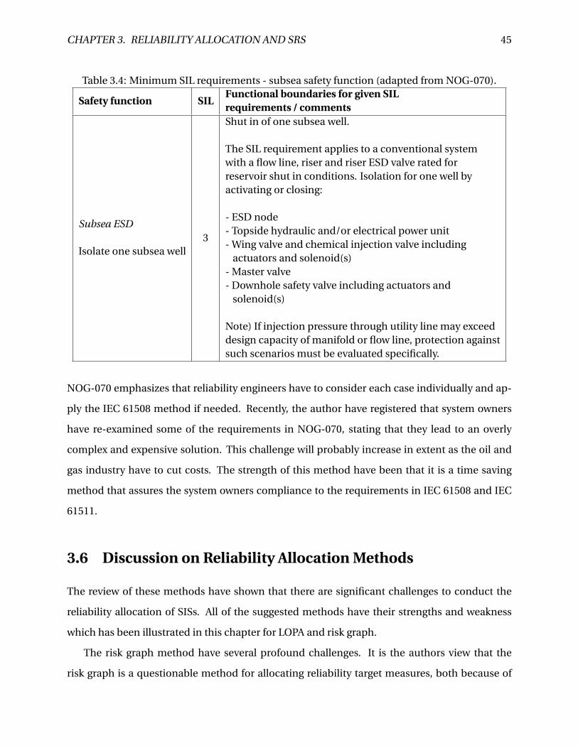
CHAPTER 3. RELIABILITY ALLOCATION AND SRS 45
Table 3.4: Minimum SIL requirements - subsea safety function (adapted from NOG-070).
Safety function SILFunctional boundaries for given SILrequirements / comments
Subsea ESD
Isolate one subsea well3
Shut in of one subsea well.
The SIL requirement applies to a conventional systemwith a flow line, riser and riser ESD valve rated forreservoir shut in conditions. Isolation for one well byactivating or closing:
- ESD node- Topside hydraulic and/or electrical power unit- Wing valve and chemical injection valve including
actuators and solenoid(s)- Master valve- Downhole safety valve including actuators and
solenoid(s)
Note) If injection pressure through utility line may exceeddesign capacity of manifold or flow line, protection againstsuch scenarios must be evaluated specifically.
NOG-070 emphasizes that reliability engineers have to consider each case individually and ap-
ply the IEC 61508 method if needed. Recently, the author have registered that system owners
have re-examined some of the requirements in NOG-070, stating that they lead to an overly
complex and expensive solution. This challenge will probably increase in extent as the oil and
gas industry have to cut costs. The strength of this method have been that it is a time saving
method that assures the system owners compliance to the requirements in IEC 61508 and IEC
61511.
3.6 Discussion on Reliability Allocation Methods
The review of these methods have shown that there are significant challenges to conduct the
reliability allocation of SISs. All of the suggested methods have their strengths and weakness
which has been illustrated in this chapter for LOPA and risk graph.
The risk graph method have several profound challenges. It is the authors view that the
risk graph is a questionable method for allocating reliability target measures, both because of

CHAPTER 3. RELIABILITY ALLOCATION AND SRS 46
its methodological challenges, and the narrow application area. This view is also supported by
Baybutt (2014) which states that: "There are multiple issues in using risk matrices and risk graphs
for SIL determination that militate against their use for this purpose. They are being pushed
beyond their natural limits. Their inherent simplifications are not consistent with other detailed
requirements of the ICE 61511..."
The minimum SIL approach is probably sufficient to achieve a tolerable risk, but it is ques-
tioned if this method will survive as it leads to overly conservative SIL requirements. The in-
dustry indicates that to strict SIL-requirements are both expensive and overly complicated. The
author also questions the statement in NOG-070 that it fulfills the PSA requirement of continu-
ous improvement. They claim compliance to this requirement as the stricter SIL requirement is
chosen if the calculated SIL is just between to SIL levels. The author believes that this is a way of
treating uncertainty more than a way to ensure system improvements. An approach based on
an as-good-as-principal seldom leads to innovative solutions.
The LOPA methodology is easier to understand and communicate. The method allows for
analyses that considers multiple parameters, such as safety and environmental impact, and
multiple barriers at the same time. The integration with HAZOP is positive as this method al-
ready is well known and a trusted analysis tool. It is the authors view that the biggest issue with
the LOPA model is that it cannot be used on SIL3 or SIL4 systems. As the industry is eager to re-
fute the conservative minimum SIL requirements the need for an easy-to-use method as LOPA
should be applicable for systems that are on the borderline between SIL2 and SIL3.
3.7 Safety Requirement Specification
When the allocation process of SIFs and the corresponding SILs is conducted, these require-
ments are adopted into the SRS. The SRS forms the basis for design and architecture of the SISs,
as well as information on how it should be operated. It is also used as the reference document
when the final validation is conducted. IEC 61508 notes that the SRS should not include any
equipment requirements. It is also important to note that the SRS only treats the SIFs, not the
other risk reduction measures that may have been introduced.
There are mainly two types of requirements in the SRS; functional requirements, and in-

CHAPTER 3. RELIABILITY ALLOCATION AND SRS 47
tegrity requirements. The content of the SRS depends on the application area, but the require-
ments in IEC 61511 are largely the same as the ones in IEC 61508. According to IEC 61508, the
functional requirements have to contain:
(a) A description of all SIFs that shall,
• provide a comprehensive detailed requirement that is sufficient to design and de-
velop a SIS that can perform the SIF.
• describe how the SISs are intended to achieve or maintain a safe state for the EUC.
• specify whether or not the SISs have to be in operation continuously or for what
periods of time they have to operate in order to achieve or maintain a safe state of
the EUC.
• specify whether the SIFs are applicable to SISs operating in low-demand, high-demand,
or continuous mode of operation.
(b) Response time performance for the SISs performing the SIFs. Example: An ABS-system
needs a short response time, a process shutdown system (PSD) can have a longer response
time.
(c) A description of the interface between the SISs and the operators.
(d) All the information that is relevant for the functional safety of an EUC that may have an
influence on the SISs design.
(e) A description of the interfaces between the SISs and any other system that is relevant for
the functional safety of the EUC. This applies for systems within, or outside, of the EUC.
(f) A description of the relevant modes of operation for the EUC, this includes:
• preparation for use of the EUC. This includes setup and adjustment.
• start-up, teach, automatic, manual, semi-automatic, steady state of operation.
• steady state for non-operation, re-setting, shut-down, and maintenance.
• the most reasonably foreseeable abnormal conditions.

CHAPTER 3. RELIABILITY ALLOCATION AND SRS 48
(g) A description of all required modes of operation of the SIS. Especially failure behavior and
requirements for response in the event of a SIS failure.
The integrity requirements have to contain (IEC 61508, 2010):
(a) The safety integrity requirements for each SIF. When required this includes the specified
target failure measure value. For low-demand mode systems this is the PFD. For high-
demand mode or continuous demand systems this is the PFH.
(b) The operational mode of the SIF.
(c) The required duty cycle and lifetime of the SIS. The duty cycle is the specific period of time
the SIS can operate.
(d) The requirements, constraints, functions, and facilities that are needed to enable proof
testing of the SIS.
(e) The most extreme of environmental conditions that the SIS may be exposed to during all
SLC phases.
(f) The electromagnetic immunity limits in order to achieve functional safety.
(g) The limiting constraint conditions for the realization of the SIS due to CCFs.
Using the SRS
There is no requirement in IEC 61508 or IEC 61511 on how to develop the SRS. The layout of
the SRS is usually chosen by the system owner and can be based on a self produced template
or guideline. An example of such a guideline for the process industry is presented in Hedberg
(2005). The SRS can also be a part of the contract between the system owner and the SIS vendor.
This way, the system owner ensures that the finished product meets the functional and integrity
requirements. The SRS is also used by the vendor under the development process when func-
tional safety assessments are conducted. An example of this is testing of performance require-
ments such as time-to-close for a valve. The final step after installing and commissioning of the

CHAPTER 3. RELIABILITY ALLOCATION AND SRS 49
SIS in the SLC is the validation process. As the SRS is only required document in IEC 61508 that
specifies the SIF requirements this document is used to validate the SIS performance.
All these aspects show that the SRS is important in order to achieve functional safety. The
main challenge in the elaboration of the SRS is to keep it clear and concise (Crosland, 2011).
This reduces the probability of misunderstandings between system owner and vendor, and min-
imizes the risk of the SIFs not being performed satisfactorily.
The SRS is not further discussed in this thesis as the author believes that the best way to do
this would be to conduct a case study and develop a proposed SRS. This task will be to compre-
hensive in this thesis given the suggested objectives.


Chapter 4
High Integrity Pressure Protection System
Case
Over the last decades the safety in the oil and gas industry has increased significantly. This is
mainly due to major accidents such as the Macondo accident (DHSG, 2011) and the Piper Alpha
accident (Cullen, 1990). These accidents have shown the potentially catastrophic consequences
that may occur. The increased safety focus has led to an increase in the use of active barriers
such as SISs described i Chapter 2.
A common type of SIS used in the oil and gas industry is a HIPPS. In this chapter, the subsea
HIPPSs installed at the Kristin field outside of Trondheim is described. The relevant demands
and SIFs are identified and the corresponding PFDavgs are determined. The uncertainty of this
reliability target measure is also discussed. At last, there is a discussion on whether or not the
HIPPS fulfills the other requirements presented in IEC 61508.
4.1 Case Description
The Kristin field is a Statoil operated gas-condensate field that is classified as a high pressure
and high temperature (HP/HT) field due to the characteristics of the reservoir, see Table 4.1.
The main installation at Kristin comprises one floating production unit (FPU), four subsea pro-
duction templates containing 12 subsea wells, and in total six flowlines (Bak et al., 2007). The
case is described by Bak et al. (2007).
51

CHAPTER 4. HIPPS CASE STUDY 52
Table 4.1: Key properties Kristin field (adapted from Bak et al., 2007).Property MeasureShut-in pressure at wellhead 740 barFlowline and riser design pressure 330 barFlowline and riser temperature 157◦ CFlowline ID from template 10 inchNumber of flowlines and HIPPS 6 pcsOverpressure acceptance criteria flowline <10−4 per yearOverpressure acceptance criteria riser <10−5 per year
High pressureLow pressure
PT
PT PT
Subsea PSD
HIPPS LS and hydraulics
PT PT
SCSSV
PMV PWV
MEG injection
MEG injection
To flowline
Figure 4.1: Principal sketch of HIPPS (inspired by Bak et al., 2007).
To reduce the cost and weight of the flowline and riser it was decided to choke the produc-
tion flow from 740 bare to approximately 300 bar, as shown in Table 4.1. This also reduces the
risk topside as the pressure of the hydrocarbon flow is reduced. However, it introduces the need
for additional protection against overpressure in the risers and flowlines. The overpressure ac-
ceptance criteria are shown in Table 4.1.
To reduce the probability of overpressure in the flowline and riser, HIPPSs are installed down-
stream of the templates. One for each flowline. The HIPPSs are installed as SISs, and are not a
part of the production control system. A principal sketch of a HIPPS is presented in Figure 4.1.
CHAPTER 4. HIPPS CASE STUDY 53
HIPPS Description
The SIF of a subsea HIPPS is: "Prevent pressure buildup in flowline and riser". The safe state of
the EUC is: "Hydracoarbon flow isolated at an acceptable pressure". These two definitions are the
author’s suggestion and are based on SINTEF (2001). The functional requirement to the SIF is
that the valve has to close within 12 seconds. It is stated in Bak et al. (2007) that this requirement
is based on the formation of hydrate plugs near the HIPPS, and that this is the main demand
for the HIPPS. However, the authors questions why a rapid closure of the topside valves is not
considered a demand for the HIPPS. This will cause a pressure build-up in the flowline and riser.
Even if the ESD starts to shut down simultaneously, it will take up to several minutes to close
the PMV or PWV. In this time the pressure build-up can be significant as the shut-in wellhead
pressure is very high. This is also supported by SINTEF (2001). As this is not conclusive for the
calculations in this chapter, and the information is limited, this issue is not further investigated.
The other requirements to the SIF proposed in Bak et al. (2007) is that it complies with SIL3
requirements in IEC 61508 and that the PFDavg < 5.0·10−4 with a test interval, τ = 8760 hours.
This PFDavg is lower than the limit given in IEC 61508. It is unknown to the author why this
is, but it may be Statoil policy to treat uncertainty in PFD calculations. This τ is used in the
calculations in Section 4.2. The HIPPS has the following subsystems (Bak et al., 2007); pressure
transmitters (PTs), logic solvers (LSs), and final elements (FEs).
PTs
Four analogue PTs in a 2oo4 configuration were chosen to achieve SIL3. Analogue PTs were
chosen as the planned shut-down system (PSD) uses digital transmitters. This reduces the prob-
ability of CCFs. A single sensor failure leads to a 1oo3 voting, and two sensor failures cause the
HIPPS to close. The sensors are located as indicated in Figure 4.1, and on top of the pipe. This
to reduce the effect of hydrate formation.
The failure modes are:
• Fail to read pressure (DU failure)
• Fail to transmit signal (DU failure)

CHAPTER 4. HIPPS CASE STUDY 54
LSs
The LSs are configured in a 1oo2 setup and certified for SIL3 application. It is assumed that
the LSs are a type A component to maximize reliability as it is located subsea inside the subsea
control module (SCM). It is tested from the topside control room through the subsea control
system. In case of replacement or modification, the SCM must be retrieved.
The failure modes are:
• Fail to read signal (DU failure)
• Fail to transmit signal (DU failure)
• Fail to interpret signal (DU failure)
FEs
The FEs consist of two equal setups; one pilot valve (PV) and one HIPPS valve. The PVs are
placed inside the SCM. If the PV fails it is assumed that it will close. This will lead to a closure of
the HIPPS as it looses the hydraulic pressure that holds the gate up.
The failure modes for the PV are:
• Fail to open (DU failure)
• Fail to close (SD failure)
• Delayed operation (DU failure)
• Internal leakage (SD failure)
• Spurious trip (SD failure)
The HIPPS valves are 10 inch valves with large actuators to enable the need for rapid clo-
sure. The valve is extensively tested for the extreme HP/HT conditions and substantial sand
production (Bak et al., 2007).
The failure modes for the HIPPS are:
• Fail to close (DU failure)

CHAPTER 4. HIPPS CASE STUDY 55
• Fail to open (DD failure)
• Delayed operation (closing > 12 secs) (DU failure)
• Leakage in closed position (SD failure, as PMV or PWV will close shortly after)
• Spurious trip (SD failure)
Testing
There are three different tests implemented in the maintenance procedures of this SIS (Bak et al.,
2007).
A proof test is conducted once per year. The test is conducted with production flow in the
flowlines. Two PTs are isolated to provoke the LS to initiate shutdown. The two remaining PTs
survey the pressure upstream and between the HIPPSs as they close. The valve position is mon-
itored to reveal if the performance requirement is met. The next step is to reveal correct PT
performance. This is done by bleeding off the pressure between the PMW and the downstream
HIPPS. The upstream shutdown valve is opened and methanol and glycol (MEG) is injected to
a pressure higher than 280 bar. All PTs shall signal to trip and close the open shutdown valve.
Finally the leakage of the HIPPSs are tested. This is done by closing the both HIPPSs and the
PMV at a pressure 70 bar lower than the wellhead pressure. MEG is injected to increase pres-
sure in front of the downstream HIPPS. The PTs between the two HIPPSs records any pressure
build-up. A pressure build-up will reveal the leakage rate of the valve. The upstream HIPPS
is tested by pressuring up downstream of the HIPPS and closing the downstream valve. If the
pressure between the two HIPPSs decrease, the upstream valve is leaking. The PTCs of this test
is considered to be 100 %. This is not realistic, but as the test procedure will cover all significant
DU failures it is a common assumption. The test period for the proof test is denoted τ1 in the
calculations.
According to Bak et al. (2007) an FMECA of the HIPPS, actuator, and hydraulic assembly
shows that the majority of dangerous failures are that the HIPPS fail to close. This have led to
the introduction of a PST. This is done by sending a signal from the control room to the LS, which
closes the HIPPS by activating the PVs. After approximately two seconds, the system is reset and
the HIPPS returns to open position. This allows for continuous production while testing, and
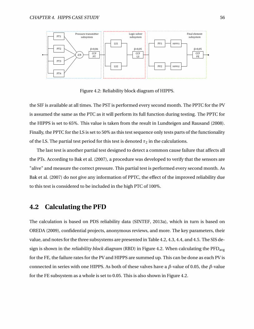
CHAPTER 4. HIPPS CASE STUDY 56
PT1
PT2
PT3
PT4
2/4CCF PT
LS1
LS2
CCF LS
PV1
PV2
HIPPS1
HIPPS2
CCF FE
Pressure transmitter subsystem
Logic solver subsystem
Final element subsystem
β=0,05β=0,06 β=0,05
Figure 4.2: Reliability block diagram of HIPPS.
the SIF is available at all times. The PST is performed every second month. The PPTC for the PV
is assumed the same as the PTC as it will perform its full function during testing. The PPTC for
the HIPPS is set to 65%. This value is taken from the result in Lundteigen and Rausand (2008).
Finally, the PPTC for the LS is set to 50% as this test sequence only tests parts of the functionality
of the LS. The partial test period for this test is denoted τ2 in the calculations.
The last test is another partial test designed to detect a common cause failure that affects all
the PTs. According to Bak et al. (2007), a procedure was developed to verify that the sensors are
"alive" and measure the correct pressure. This partial test is performed every second month. As
Bak et al. (2007) do not give any information of PPTC, the effect of the improved reliability due
to this test is considered to be included in the high PTC of 100%.
4.2 Calculating the PFD
The calculation is based on PDS reliability data (SINTEF, 2013a), which in turn is based on
OREDA (2009), confidential projects, anonymous reviews, and more. The key parameters, their
value, and notes for the three subsystems are presented in Table 4.2, 4.3, 4.4, and 4.5. The SIS de-
sign is shown in the reliability block diagram (RBD) in Figure 4.2. When calculating the PFDavg
for the FE, the failure rates for the PV and HIPPS are summed up. This can be done as each PV is
connected in series with one HIPPS. As both of these valves have a β-value of 0.05, the β-value
for the FE subsystem as a whole is set to 0.05. This is also shown in Figure 4.2.

CHAPTER 4. HIPPS CASE STUDY 57
Table 4.2: Reliability data for PT (adapted from SINTEF, 2013a).Parameter Value NoteλDU 0.5·10−6/h 4.1.3 in SINTEF (2013a).SFF 77%PTC 100% No information given. Assumption.β 0.06
Table 4.3: Reliability data for LS (adapted from SINTEF, 2013a).Parameter Value NoteλDU 0.11·10−6/h No LS subsea data. Inc. 4.2.3.1-4.2.3.3 in SINTEF (2013a).SFF 91%PTC 100% No information given. Assumption.PPTC 50% No information given. Assumption.β 0.03 Low estimate as a hardwired LS is assumed.
Table 4.4: Reliability data for pilot valve (adapted from SINTEF, 2013a).Parameter Value NoteλDU 0.10·10−6/h Included reliability improvement due to partial test.SFF 60%PTC 100% No information given. Assumption.PPTC 100% Is fully tested during PST of the HIPPS valve.β 0.05 Low estimate as each pilot valve only control one HIPPS.
Table 4.5: Reliability data for HIPPS valve (adapted from SINTEF, 2013a).Parameter Value NoteλDU 1.50·10−6/h Not subsea HIPPS data. 4.3.3 in SINTEF (2013a). Probably to high.SFF 61%PTC 100% No information given. Assumption.PPTC 65% Assumption based on Lundteigen and Rausand (2008).β 0.05

CHAPTER 4. HIPPS CASE STUDY 58
Calculations
All PFDs in the calculations are average values. The PST of the HIPPS is not included in the first
calculation. The individual PFDavg are calculated:
PFD(i )PT(2oo4) = [(1−β) ·λDU ·τ1]3 = [(1−0.06) ·0.50 ·10−6 ·8760]3 = 0.07 ·10−6 (4.1)
PFD(i )LS(1oo2) =
[(1−β) ·λDU ·τ1]2
3= [(1−0.03) ·0.11 ·10−6 ·8760]2
3= 0.29 ·10−6 (4.2)
PFD(i )FE(1oo2) =
[(1−β) ·λDU ·τ1]2
3= [(1−0.05) · [(0.10+1.50) ·10−6] ·8760]2
3= 5.910 ·10−5 (4.3)
The next step is to calculate the PFDavg contribution due to CCFs:
PFD(CCF)PT(2oo4) =Ckoon ·β · λDU ·τ1
2= 1.1 ·0.06 · 0.50 ·10−6 ·8760
2= 1.4454 ·10−4 (4.4)
PFD(CCF)LS(1oo2) =Ckoon ·β · λDU ·τ1
2= 1.0 ·0.03 · 0.11 ·10−6 ·8760
2= 1.445 ·10−5 (4.5)
PFD(CCF)FE(1oo2) =Ckoon ·β · λDU ·τ1
2= 1.0 ·0.05 · (0.10+1.50) ·10−6 ·8760
2= 3.5040 ·10−4 (4.6)
The PFDavg is calculated for each subsystem:
PFDPT(2oo4) = PFD(i )PT(2oo4) +PFD(CCF)
PT(2oo4) = 0.07 ·10−6 +1.4454 ·10−4 = 1.4461 ·10−4 (4.7)

CHAPTER 4. HIPPS CASE STUDY 59
PFDLS(1oo2) = PFD(i )LS(1oo2) +PFD(CCF)
LS(1oo2) = 0.29 ·10−6 +1.445 ·10−5 = 1.474 ·10−5 (4.8)
PFDFE(1oo2) = PFD(i )FE(1oo2) +PFD(CCF)
FE(1oo2) = 5.910 ·10−5 +3.5040 ·10−4 = 4.095 ·10−4 (4.9)
The total PFDavg for the SIS is:
PFDavg = PFDPT(2oo4) +PFDLS(1oo2) +PFDFE(1oo2) = 5.69 ·10−4 (4.10)
Results
The PFDavg for the HIPPS system is 5.69·10−4. Comparing this result with the PFD requirements
table in Table 2.1, the SIS classifies as a SIL3 system. However, it is stated in the integrity require-
ments in Bak et al. (2007) that the PFDavg should be lower than 5.0·10−4. It is possible that this
was reason that the PST described in Section 4.1 was introduced. To see the effect of the PST
to the PFDavg an Excel worksheet was developed. PTC formulas provided by Rausand (2014,
p.351) were used. As the proof test in this case is considered to be perfect, it is the PST that is
considered.
By applying the PPTCs discussed in Section 4.1, the PFDavg was calculated to 3.14·10−4. This
reduces the PFDavg to an acceptable level according to Bak et al. (2007). The PST has lowered the
PFDavg but not by much. Table 4.6 shows some key parameters with varying PPTC of the HIPPS.
The PPTCs for the PTs and LSs are kept constant. Table 4.6 shows that the PFD contribution
from the different subsystems is altered with varying PPTC. For low coverage, the dominant PFD
contributors are the HIPPSs. This was anticipated as the failure rate for this element is a 10 fold
higher than the other elements. However, as the PPTC increases the biggest PFD contributors
are the PTs. This is clearly because the PPTC of the PTs is kept constant, while the PFDavg for the
HIPPSs will be reduced as the PPTC increases. The contribution from PFDCCF increases as the

CHAPTER 4. HIPPS CASE STUDY 60
Table 4.6: Key parameters with varying PPTC for the FEs.Parameter No PST PPTC 40% PPTC 65% PPTC 90%PFDavg 5.69·10−4/h 3.95·10−4/h 3.14·10−4/h 2.41·10−4/hPFDPT in % 25,4% 36.6% 46.0% 60.1%PFDLS in % 2,6% 2.2% 2.7% 3.5%PFDFE in % 72,0% 61.2% 51.3% 35.6%PFDCCF in % 89,6% 95.2% 97.7% 99,2%PFDi in % 10,4% 4.8% 2.3% 0,8%
PPTC increases. The PFD contribution from the LSs are very low in all configurations.
The calculations show that the SIS is able to fulfill the integrity requirements set in Bak et al.
(2007). A PST will improve the PFDavg satisfactorily with the PPTC proposed in Section 4.1.
4.3 Uncertainty in PFD Calculation
Reliability assessments, such as the calculation of PFDavg, are conducted to form a basis for
decision-making. However, people in charge of taking decisions are rarely reliability analysts.
Therefore, it can be useful to substantiate the assessments with an evaluation of the uncertainty.
This section contains some thoughts on uncertainty related to the HIPPS case described in Sec-
tion 4.1. A common classification of uncertainty is (NUREG-1855, 2009):
• Epistemic uncertainty: Uncertainty due to lack of knowledge on how to describe the per-
formance of a system or a process (Jin et al., 2012). A measure of how certain the analyst
is that the system being assessed is understood and represented precisely. Epistemic un-
certainty is again divided into three sub categories:
– Completeness uncertainty
– Model uncertainty
– Parameter uncertainty
• Aleatory uncertainty: Uncertainty related to random events like such as initiating events
or component failures. These are natural inherent processes that cannot be reduced.
However, as mentioned in Jin et al. (2012), improved knowledge on fundamentals of natu-
ral phenomena will lead to a transition from aleatory uncertainty to epistemic uncertainty.

CHAPTER 4. HIPPS CASE STUDY 61
A reliability assessment is usually founded on various statistical models. As an example, the
calculation in Section 4.2 assumes constant failure rates. This is an assumption that enables
modeling of the failure rate to assess it mathematically. Unfortunately, both the assumption of
constant failure rate and the data used to build this model are sources of uncertainty as they will
only partly describe the behavior of the system. This is the epistemic uncertainty that could be
addressed in an uncertainty assessment. The aleatory uncertainty is usually not relevant, nor
possible, to assess in a reliability analysis perspective. It can be argued that a reliability analysis
as a whole will express the aleatory uncertainty of a certain system.
Parameter Uncertainty
Parameter uncertainty relates to the uncertainty of parameter values. In the HIPPS case, ele-
ment failure rates, β-values, and PPTC values are examples of such parameters. Within these
parameters there are different causes of the uncertainty. Jin et al. (2012) mention an issue that
is highly relevant for SISs. They are very reliable and designed for operation in up to 30 years.
Therefore, the failure rate data used to design new SISs is based on failures of elements that may
be 30 years old. A different type of parameter uncertainty can be described by assessing the β-
value. CCFs are considered to be a significant PFD contributor (Lundteigen and Rausand, 2007).
This increases the importance of a thorough assessment of the β-value. This value depends on
the SIS design. It is also strongly dependent on operational and environmental conditions. This
makes the assessment of this parameter very challenging as the dependency between elements
is hard to quantify. Table 4.6 shows that given a PPTC of 65%, the PFD contributions due to CCFs
is 97.7%. This indicates that a small variation in theβ-value has a strong impact on the reliability
assessment. Jin et al. (2012) mention complexity in SIS design as a contributor to uncertainty,
and as the complexity of SISs increases so does the importance of CCFs and β-values. Vaurio
(2005) discusses the challenge of uncertainty in CCF quantification and presents a methodol-
ogy to account for this. The PDS data handbook (SINTEF, 2013a) is the source for β-values in
Section 4.6. It states that: "The beta values are based on expert judgments and some operational
experience." It is also mentioned that these values have been slightly increased due to results
from recent operational reviews. These statements illustrate that there is uncertainty related
to the β-values, but there is not suggested any method to assess the uncertainties in the PDS-

CHAPTER 4. HIPPS CASE STUDY 62
handbook SINTEF (2013a), nor in IEC 61508. However, IEC 61508 introduces a "70% -rule" for
the calculations of PFDavg, meaning that they require that the failure rates that are used to have
a 70% confidence interval. This is not a requirement that considers the specific uncertainty in
each case, but adds conservatism in the calculations.
Model Uncertainty
Model uncertainty is a result of simplifications and assumptions made to enable modeling of
a certain process. The example of component characterization models such as the exponen-
tial distribution model is already mentioned. In Section 2.3, some assumptions for utilizing
the simplified formulas by Rausand and Høyland (2004) was mentioned. All SIS elements are
considered to have a constant failure rate. In other words, degradation of elements is not con-
sidered. Jin et al. (2012) specifically mention the challenge regarding this assumption in subsea
applications. This is because intervention, such as preventive maintenance actions, is expen-
sive, and is therefore reduced to a minimum in the design process. Some of these elements may
be degraded due to the pressure or the corrosive environment. This illustrates the uncertainty
assumptions in models can cause.
Model uncertainty can be improved by addressing some of these assumptions. An exam-
ple is the PTC. A common assumption was that the PTC was 100%, meaning that all possible
faults are detected in a proof test. This assumption is obviously not achievable for all systems.
Therefore, to improve the calculations, and reduce uncertainty, PTC can now be included in the
calculation of PFDavg (see e.g., Rausand, 2014). This improves model uncertainty, but it also in-
troduce a new parameter uncertainty that have to be evaluated. It is the authors opinion that
parameter uncertainties, such as PTC, is easier to investigate and communicate, than inherent
model uncertainties.
Completeness Uncertainty
Completeness uncertainty describes uncertainty that is not properly included in an analysis (Jin
et al., 2012). Some of these uncertainties are deliberately not treated. There are many reasons
why this is decided, but time or cost constraints are probably the most apparent. This uncer-

CHAPTER 4. HIPPS CASE STUDY 63
tainty should not be critical as it is known, but it can also be neglected from an analysis due
to lack of competence on how to treat it. As mentioned earlier, the operating environment of a
subsea installation will have an effect of the reliability of certain mechanical components. The
engineers that designs the installation know about the potential additional degradation this op-
erating environment can cause, but as it can be difficult to quantify this affect it is neglected.
Another and perhaps more challenging type of uncertainty is called the unknown complete-
ness uncertainty. An example of this is the use of new technology, and how new components
introduce new failure modes or failure mechanisms. This is probably some of the reason that
route 1H distinguishes between type A and type B elements as described in Section 2.4. Hu-
man and organizational factors have not been discussed in this thesis, but are factors that may
introduce uncertainty in SIS reliability assessments (Jin et al., 2012).
Discussion
There are several types of uncertainty that affect reliability assessments. The most common
sources of uncertainty is presented. It is important to note that not all reliability assessments
should include an uncertainty assessment. Reliability analysts should however address the
uncertainty to decision-makers. Regarding the case presented in this chapter, the calculated
PFDavg was barely better than the stated requirement of 5.0·10−4 per hour. In the authors opin-
ion, this is an example where uncertainty assessment should be conducted. Mainly because the
calculated PFDavg was close to the integrity requirements. Two other important aspects is that
the SIS is a critical system to achieve functional safety, and that the installation is mounted sub-
sea making potential modifications very expensive. Methods used to quantify the uncertainty
in reliability assessments are not presented as this will be time consuming and go beyond the
scope of this thesis.
4.4 Evaluating Non-Integrity Requirements
Besides the integrity requirements for the SIS, IEC 61508 gives requirements to both architec-
ture and treatment of systematic faults. As the specific case in this thesis does not include any
information of treatment of systematic faults, the fulfillment of the architectural constraints is

CHAPTER 4. HIPPS CASE STUDY 64
Table 4.7: Achievable SIL for the SIS elements.Element SFF HFT Type Achievable SIL
PT 77% 2 A SIL4LS 91% 1 A SIL4PV 60% 0 A SIL2
HIPPS 61% 0 A SIL2
discussed in this section. The case does not contain any operational data for the installed equip-
ment. Therefore, route 1H is applied. Route 2H cannot be chosen as this requires simulation to
verify the confidence of the PFDavg as described in Section 2.4.
The first step is to assess and classify the subsystem elements. Bak et al. (2007) states that the
PTs can be regarded as "proven in use". According to the definition of this term in IEC 61508,
this implies that it fulfills the requirements for a type A element. As stated in Bak et al. (2007),
the LS is certified for SIL3 application. It is assumed that the LS can be regarded as a type A
element. The LS is positioned in the SCM, which makes it unavailable for repair. It is likely
that this calls for a reliable LS with an extensive operational experience. There is very limited
information on the PV, but as this is a common equipment especially in subsea installations, it
is considered as a type A element. Finally, the HIPPS valves are considered a type A element. This
is not obvious as it is stated in SINTEF (2001) that Kristin was the first field in the north sea that
applied subsea HIPPS. This means that there was a lack of operational experience. In addition,
the HP/HT conditions and a relatively high sand production can lead to failures that are not
considered in the design phase. However, the failure modes of the valve are well known. Bak
et al. (2007) also state that the HIPPS is extensively tested, and the HIPPS failure rate is relatively
conservative. The second step of route 1H is to determine the SFF. The SFFs for the different
subsystems are given in Table 4.2, 4.3, 4.4, and 4.5. These are taken from SINTEF (2013a). The
next step is to determine the achievable SIL for each subsystem. This is achieved by considering
the requirements in Table 2.1. The achievable SILs are given in Table 4.7.
The final step of the process is to determine the achievable SIL for the whole SIF. This can be
done by reducing the RBD in Figure 4.2 according to the rules given in Section 2.4. The result of
this process is that the SIF can operate SIL3 This is shown in Figure 4.3. There are a few issues
that needs to be commented. Firstly, it is the already discussed categorization of the HIPPS. If
this valve was considered a type B element, the highest achievable SIL would be SIL2. Secondly,
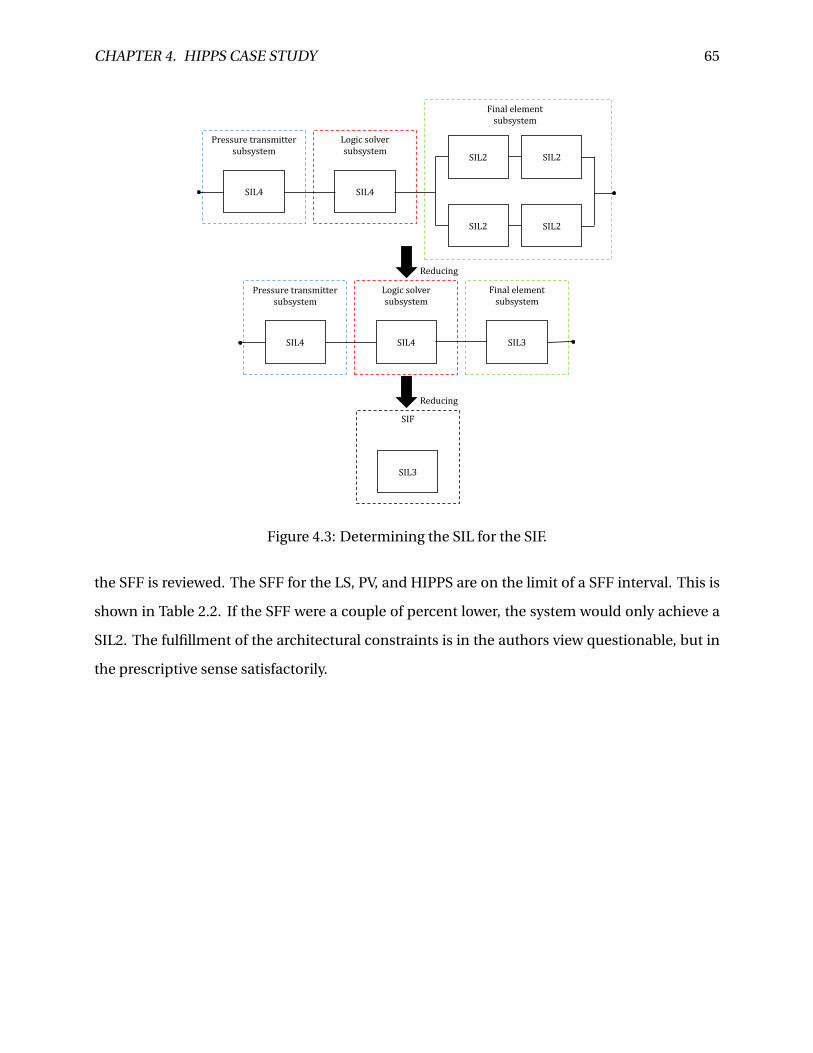
CHAPTER 4. HIPPS CASE STUDY 65
SIL4
Pressure transmitter subsystem
Logic solver subsystem
Final element subsystem
SIL4
SIL2
SIL2
SIL2
SIL2
SIL4
Pressure transmitter subsystem
Logic solver subsystem
Final element subsystem
SIL4 SIL3
Reducing
SIL3
Reducing
SIF
Figure 4.3: Determining the SIL for the SIF.
the SFF is reviewed. The SFF for the LS, PV, and HIPPS are on the limit of a SFF interval. This is
shown in Table 2.2. If the SFF were a couple of percent lower, the system would only achieve a
SIL2. The fulfillment of the architectural constraints is in the authors view questionable, but in
the prescriptive sense satisfactorily.


Chapter 5
Summary and Recommendations for
Further Work
5.1 Summary and Conclusions
SISs are technical systems designed to improve functional safety of a system. IEC 61508 is used
to ensure a reliable SIS. Extensive knowledge of concepts and terminology in IEC 61508 is neces-
sary to achieve compliance. Achieving this knowledge is the first objective in this thesis. Chap-
ter 2 explains how SISs are designed and tested, presents the SLC, and gives an introduction to
the various requirements in IEC 61508. An introduction to the quantification of PFDavg and PFH
is also given.
The second objective in this thesis is to describe relevant approaches for SIL allocation, and
discuss the pros and cons of these methods. An introduction to SIL allocation as a concept is
given in Chapter 2. Further, three methods are chosen for a more thorough description. The risk
graph method and LOPA was chosen as they have been extensively debated and represent two
fundamentally different methodologies. The minimum SIL approach was included to illustrate
that SIL allocation in practice may vary from the risk-based approach suggested in IEC 61508.
It is necessary to thoroughly investigate what the required input of this process is. This will
vary depending on the chosen method. The risk graph method is based on the knowledge of
risk factors, and how they influence an accident scenario. The starting point of this analysis is
an end event. According to the author, this strongly limits the applicability for the risk graph. If
67

CHAPTER 5. SUMMARY 68
there are few HEs that are relevant for the determination of the SIL, the method can be applied.
However, if the number of HE is large, the number of end events, and hence the number of
iterations needed in the risk graph procedure, will be unmanageable. The risk graph is presented
in Section 3.3.
The LOPA procedure is described and discussed in Section 3.4. The LOPA methodology is
based on the initiating events. Rausand (2011) introduces a procedure similar to a risk assess-
ment methodology and is therefore easier to communicate and understand than the risk graph
procedure. The possibility to integrate the LOPA with a HAZOP is also considered as a clear
strength. However, the method is limited to SIL2 applications due to uncertainty in the semi-
quantitative methodology. An introduction to the minimum SIL approach suggested by NOG-
070 (2004) debates if this method is starting to be outdated as it often leads to conservative SIL
requirements. Higher SIL requirements leads to higher cost. The author is under the impression
that the oil- and gas industry in particular may disregard this method to save costs.
The third objective is to list the main elements of a typical SRS. This is done in Section 3.7.
A brief discussion on the use of a SRS is also provided. The topic is not further examined as it is
the authors opinion that the outcome would be limited unless a case study was conducted.
Chapter 4 presents the HIPPS case study from the Kristin subsea field outside Trondheim.
The demand for the SIF is discussed. This is also a part of objective four. However, as little infor-
mation is given in Bak et al. (2007) regarding HIPPS demands for this specific case the discussion
is limited. Section 4.2 contains the reliability data for the SIS elements, and the calculation of
the PFDavg. The calculations show that the system meets the SIL3 requirements. However, the
requirement in Bak et al. (2007) of a PFDavg lower than 5.0·10−4 is not achieved without intro-
ducing the PST. It is examined how sensitive the PFDavg is to the PST parameters, such as the
PPTC. With a PPTC of the HIPPS valves of 65% all requirements in Bak et al. (2007) are met.
CCFs constitute between 90-99% of the total PFDavg depending on the PPTC. The calculations
constitute the second part of objective four.
The fifth objective is to discuss whether the HIPPS fulfills the other requirements presented
in IEC 61508. As the case study does not contain any information on how to avoid and control
systematic failures, this task is reduced to discuss the compliance with the architectural con-
straints. This discussion is presented in Section 4.4. The SIS does achieve a SIL3. However, the

CHAPTER 5. SUMMARY 69
information in Bak et al. (2007) does not provide any convincing evidence that the HIPPS valves
can be classified as type A elements. The end result is therefore questionable.
The sixth, and final, objective is to discuss the uncertainties related to the calculated PFDavg
for the HIPPS. This discussion is presented in Section 4.3. The different categories of epistemic
uncertainties is debated. It is the authors view that the parameter uncertainties and model un-
certainties will be the largest contributors to uncertainty in PFDavg calculations. The β-value
has a strong effect on the PFDavg and should be assessed individually for SISs that have to fulfill
SIL3 requirements.
The author thinks it would be preferable to establish contact with the Statoil to get more
details for the case study. This would have reduced the necessary assumptions, and been a
better basis for discussions.
5.2 Recommendations for Further Work
Based on the author’s experience during the preparation of this thesis, some topics recom-
mended for further work are:
• Conduct a SIL allocation study using the LOPA methodology on a SIL3 SIS. Assess the
uncertainty in the calculations and discuss the applicability of LOPA on SIL3 SISs.
• Develop an uncertainty assessment procedure for SIL assessments. It is clear that the
uncertainty in calculations should be addressed in some cases. A procedure on suggested
methods to apply, and what types of uncertainty to assess could be useful.
• Assessing the transition of uncertainties from model uncertainties to parameter uncer-
tainties. Does the introduction of new parameters that reduce model uncertainty reduce
the overall uncertainty? Or is the knowledge on the parameters, such as the PPTC, too
limited to conduct a satisfactorily evaluation?


Appendix A
Acronyms
ALARP As low as reasonable possible
BPCS Basic process control system
CCF Common cause failure
DC Diagnostic coverage
DD Dangerous detected
DHSV Downhole safety valve
DU Dangerous undetected
ESD Emergency shutdown system
ETA Event tree analysis
EUC Equipment under control
FAR Fatal accident rate
FE Final element
FMECA Failure modes, effects, and criticality analysis
FPU Floating production unit
71

APPENDIX A. ACRONYMS 72
FTA Fault tree analysis
FTF Fail to function
HAZID Hazard identification
HAZOP Hazard and operability study
HE Hazardous event
HFT Hardware fault tolerance
HIPPS High integrity pressure protection system
HP/HT High pressure / high temperature
IPK Department of Production and Quality Engineering (Norwegian abbreviation for "Institutt
for Produksjons- og Kvalitetsteknikk")
IRPA Individual risk per annum
LOPA Layers of protection analysis
LS Logic solver
MEG Methanol and glycol
MRT Mean repair time
MTTF Mean time to failure
MTTR Mean time to repair
NTNU Norwegian University of Science and Technology (Norwegian abbreviation for "Norges
Teknisk-naturvitenskapelige Universitet")
OREDA Offshore reliability data
PFD Probability of failure on demand
PFH Probability of a dangerous failure per hour

APPENDIX A. ACRONYMS 73
PMV Production master valve
PPTC Partial proof test coverage
PSA Petroleum Safety Authority
PSD Process shutdown system
PST Partial stroke testing
PT Pressure transmitter
PTC Proof test coverage
PV Pilot valve
PWV Production wing valve
QRA Quantitative risk analysis
RAMS Reliability, availability, maintainability, and safety
RBD Reliability block diagram
SCM Subsea control module
SD Safe detected
SFF Safe failure fraction
SIF Safety instrumented function
SIL Safety integrity level
SIS Safety instrumented system
SLC Safety life cycle
SRS Safety requirement specification
ST Spurious trip

APPENDIX A. ACRONYMS 74
SU Safe undetected
SWIFT Structured what-if technique
TMEL Target mitigated event likelihood

Bibliography
Bak, L., Sirevaag, R., and Stokke, H. (2007). HIPPS protects subsea prodction in HP/HT cond-
tions. Offshore Magazine, 67.
Baum, D., Faulk, N., and Pèrez, P. J. (2009). Improved integration of LOPA with HAZOP analyses.
Proc. Safety Prog., 28(4):308–311.
Baybutt, P. (2007). An improved risk graph approach for determination of safety integrity levels
(SILs). Proc. Safety Prog., 26(1):66–76.
Baybutt, P. (2012). Using risk tolerance criteria to determine safety integrity levels for safety
instrumented functions. Journal of Loss Prevention in the Process Industries, 25(6):1000–1009.
Baybutt, P. (2014). The use of risk matrices and risk graphs for SIL determination. Proc. Safety
Prog., 33(2):179–182.
Bingham, K. (2007). Integrating HAZOP and LOPA can result in exceptional benefits. Process-
West, pages 38–39.
BP (2006). Guidance on practice of layer of protection analysis (LOPA). Tecnhical report GP
48-03, BP Group, London.
CCPS (1993). Guidelines for Safety Automation of Chemical Processes. Center for Chemical Pro-
cess Safety, American Institute of Chemical Engineers, New York.
CCPS (2001). Layer of Protection Analysis: Simplified Process Risk Assessment. Center for Chem-
ical Process Safety, American Institute of Chemical Engineers, New York.
75

BIBLIOGRAPHY 76
CCPS (2010). Guidelines for Process Equipment Reliability Data: with Data Tables. Center for
Chemical Process Safety, American Institute of Chemical Engineers, New York.
Crosland, A. (2011). The importance of a clear safety requirements specification as part of the
overall safety lifecycle. Safety Control Systems Conference - IDC Tecnhologies. Emerson Process
Management.
Cullen, W. D. L. (1990). Theprocess Inquiry into the Piper Aalpa Disaster. Department of Energy,
London, UK.
DHSG (2011). Final report on the investigation of the Macondo well blowout. Deepwater Hori-
zon Study Group, Center for Catastrophic Risk Management.
EXIDA (2007). Safety equipment reliability handbook.
Hedberg, J. (2005). Safety requirements specifications, guidline. Process industry - IEC 61511,
SP Swedish National Testing and Research Institute, Sweden.
Hokstad, P. and Corneliussen, K. (2004). Loss of safety assessment and the IEC61508 standard.
Reliability Engineering & System Safety, 83(1):111–120.
IEC 61508 (2010). Functional Safety of Electical/Electronic/Programmable Electronic Safety-
Related Systems, Part 1-7. International Electrotechnical Commission, Geneva.
IEC 61511 (2003). Functional Safety: Safety Instrumented Syystems for the Process Industry Sector,
Part 1-3. International Electrotechnical Commission, Geneva.
IEC 62061 (2005). Safety of Machinery - Functional Safety of Safety-related Electrical, Electronic
and Programmable Electronic Control Systems. International Electrotechnical Commission,
Geneva.
Jin, H., Lundteigen, M. A., and Rausand, M. (2012). Uncertainty assessment of reliability es-
timates for safety-instrumented systems. Proceedings of the Institution of Mechanical Engi-
neers, Part O: Journal of Risk and Reliability, 226(6):646–655.
Lundteigen, M. A. . (2009). Safety instrumented systems in the oil and gas industry: concepts
and methods for safety and reliability assessments in design and operation.

BIBLIOGRAPHY 77
Lundteigen, M. A. and Rausand, M. (2006). Assessment of hardware safety integrity require-
ments. pages 195–98, Ispra, Italy. ESReDA, European Commision, Joint Research Centre.
Lundteigen, M. A. and Rausand, M. (2007). Common cause failures in safety instrumented sys-
tems on oil and gas installations: Implementing defense measures through function testing.
Journal of Loss Prevention in the Process Industries, 20(3):218–229.
Lundteigen, M. A. and Rausand, M. (2008). Partial stroke testing of process shutdown valves:
How to determine the test coverage. Journal of Loss Prevention in the Process Industries,
21(6):579–588.
MIL-STD-882D (2000). Standard Practice for System Safety. U.S. Department of Defence, Wash-
ington D.C.
Nait-Said, R., Zidani, F., and Ouzraoui, N. (2009). Modified risk graph method using fuzzy rule-
based approach. Journal of Hazardous Materials, 164(2-3):651–658.
NOG-070 (2004). Application of IEC 61508 and IEC 61511 in the Norwegian Petroleum Industy.
The Norwegian Oil and Gas Association, Stavanger, Norway.
NS 5814 (2008). Requirements for Risk Assessment. Standard Norge, Oslo, Norway, Norwegian
edition.
NUREG-1855 (2009). Guidance on how the Treatment of Uncertanties Associated with PRAs in
Risk-Informed Decision Making. U.S Nuclear Regulatory Commission, Office of Nuclear Reg-
ulatory Research, Washington, DC.
OREDA (2009). OREDA Reliability Data. OREDA Participants, 4 edition. Available from: Det
Norske Veritas, NO 1322 Høvik, Norway.
Rausand, M. (2011). Risk assessment: Theory, Methods, and Applications. Wiley, Hoboken, N.J.
Rausand, M. (2014). Reliability of Safety-Critical Systems: Theory and Applications. Wiley, Hobo-
ken, N.J.
Rausand, M. and Høyland, A. (2004). System Reliability Theory: Models, Statistical, Methods, and
Applications. Wiley, Hoboken, NJ, 2 edition.

BIBLIOGRAPHY 78
Salis, C. (2011). Using Risk Graphs for Safety Integrity Level (SIL) assessment - a user-guide for
chemical engineers. IChemE, London, England.
Signoret, J.-P. (2007). High integrity pressure proctection systems (HIPPS) - making SIL calcula-
tions effective. Exploration and Production - oil and gas review (OTC edition), pages 14–17.
SINTEF (2001). Use of HIPPS for equipment protection. Stf38 a01422, SINTEF Safety Research.
SINTEF (2013a). Reliability data for safety instrumented systems, pds data handbook. Hand-
book STF A24443, SINTEF Safety Research, Trondheim, Norway.
SINTEF (2013b). Reliability prediction method for safety instrumented systems: PDS method
handbook. Handbook STF A24443, SINTEF Safety Research, Trondheim, Norway.
Sklet, S. (2006). Safety barriers: Definition, classification, and performance. Journal of Loss
Prevention in the Process Industries, 19(5):494–506.
Smith, D. and Simpson, K. (2011). Safety Critical Systems Handbook: A Straightforward Guide
to Functional Safety: IEC 61508 and Related Standard. Elsevier: Butterworth Heinemann,
Oxford, 3 edition.
Summers, A. E. (2003). Introduction to layers of protection analysis. Journal of Hazardous Ma-
terials, 104(1-3):163–168.
Vaurio, J. K. (2005). Uncertainties and quantification of common cause failure rates and proba-
bilities for system analyses. Reliability Engineering & System Safety, 90(2-3):186–195.

Curriculum Vitae
Name: Jon Mikkel Haugen
Gender: Male
Date of birth: 7. March 1987
Address: Nardovegen 15A, 7032 Trondheim
Home address: Fløtlivegen 218, 2390, Moelv
Nationality: Norwegian
Email: [email protected]
Telephone: +47 48607926
Language Skills
Native language is Norwegian. Written and spoken English sufficient for most purposes.
Education
08.2008-12.2014: Norwegian University of Science and Technology
08.2003-06.2006: Ringsaker Videregående Skole
Experience
06.2013-08.2013: Summer intern, Norconsult AS (Sandvika)
01.2012-12.2012: Vice president academic affairs, Student Union, NTNU (Trondheim)
06.2011-08.2011: Summer intern, Itella Information (Oslo)
79

BIBLIOGRAPHY 80
04.2007-10.2007: Agricultural exchange program, Fargo ND (USA)
06.2006-07.2008: Part time employee, Sport1 Superstore (Hamar)
Computer Skills
• MS Office
• LaTex
Hobbies and Other Activities
I enjoy the company of family and friends. I also enjoy training and sports in general. Mountain
hiking and fishing for trout in the mountains is my favorite way of relaxing and recharging.