Embed Size (px)
Citation preview

pychemia DocumentationRelease 0.1.2
Guillermo Avendano-Franco
Nov 09, 2018

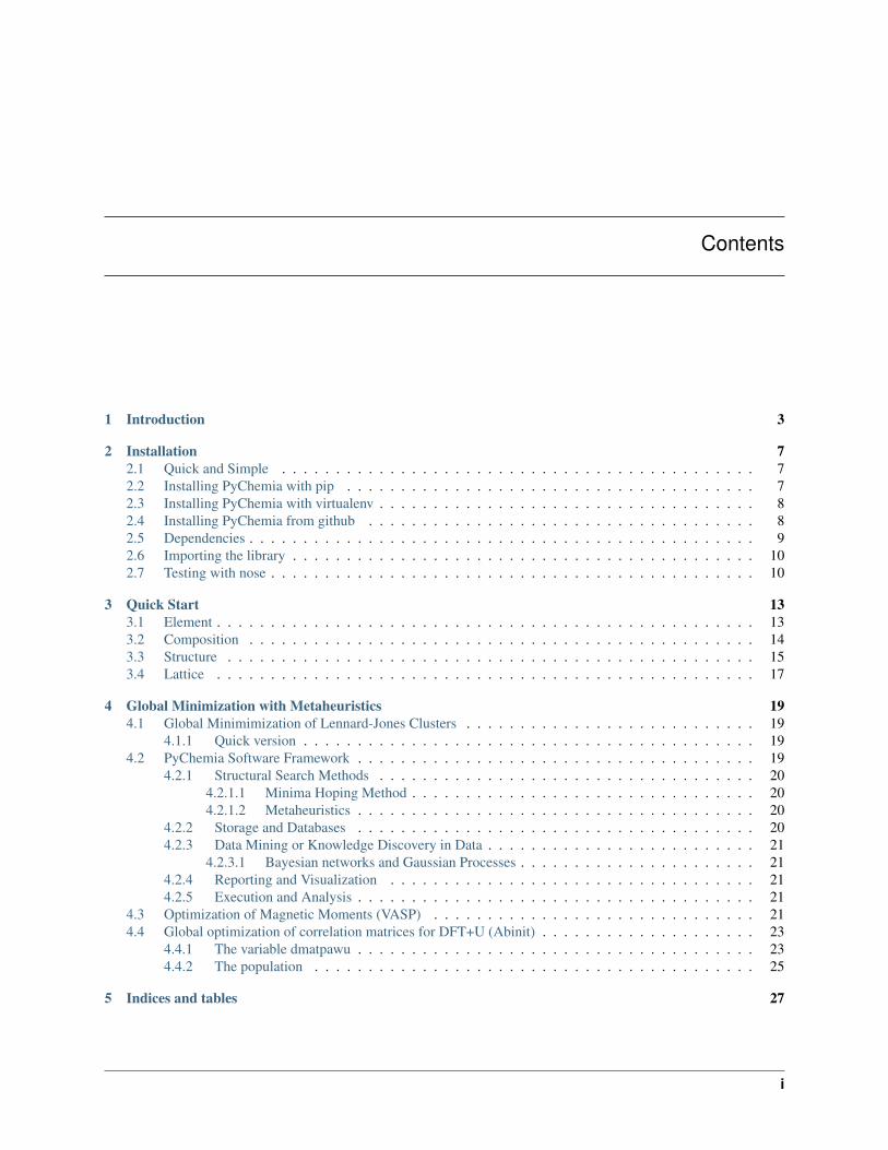
Contents
1 Introduction 3
2 Installation 72.1 Quick and Simple . . . . . . . . . . . . . . . . . . . . . . . . . . . . . . . . . . . . . . . . . . . . 72.2 Installing PyChemia with pip . . . . . . . . . . . . . . . . . . . . . . . . . . . . . . . . . . . . . . 72.3 Installing PyChemia with virtualenv . . . . . . . . . . . . . . . . . . . . . . . . . . . . . . . . . . . 82.4 Installing PyChemia from github . . . . . . . . . . . . . . . . . . . . . . . . . . . . . . . . . . . . 82.5 Dependencies . . . . . . . . . . . . . . . . . . . . . . . . . . . . . . . . . . . . . . . . . . . . . . . 92.6 Importing the library . . . . . . . . . . . . . . . . . . . . . . . . . . . . . . . . . . . . . . . . . . . 102.7 Testing with nose . . . . . . . . . . . . . . . . . . . . . . . . . . . . . . . . . . . . . . . . . . . . . 10
3 Quick Start 133.1 Element . . . . . . . . . . . . . . . . . . . . . . . . . . . . . . . . . . . . . . . . . . . . . . . . . . 133.2 Composition . . . . . . . . . . . . . . . . . . . . . . . . . . . . . . . . . . . . . . . . . . . . . . . 143.3 Structure . . . . . . . . . . . . . . . . . . . . . . . . . . . . . . . . . . . . . . . . . . . . . . . . . 153.4 Lattice . . . . . . . . . . . . . . . . . . . . . . . . . . . . . . . . . . . . . . . . . . . . . . . . . . 17
4 Global Minimization with Metaheuristics 194.1 Global Minimimization of Lennard-Jones Clusters . . . . . . . . . . . . . . . . . . . . . . . . . . . 19
4.1.1 Quick version . . . . . . . . . . . . . . . . . . . . . . . . . . . . . . . . . . . . . . . . . . 194.2 PyChemia Software Framework . . . . . . . . . . . . . . . . . . . . . . . . . . . . . . . . . . . . . 19
4.2.1 Structural Search Methods . . . . . . . . . . . . . . . . . . . . . . . . . . . . . . . . . . . 204.2.1.1 Minima Hoping Method . . . . . . . . . . . . . . . . . . . . . . . . . . . . . . . . 204.2.1.2 Metaheuristics . . . . . . . . . . . . . . . . . . . . . . . . . . . . . . . . . . . . . 20
4.2.2 Storage and Databases . . . . . . . . . . . . . . . . . . . . . . . . . . . . . . . . . . . . . 204.2.3 Data Mining or Knowledge Discovery in Data . . . . . . . . . . . . . . . . . . . . . . . . . 21
4.2.3.1 Bayesian networks and Gaussian Processes . . . . . . . . . . . . . . . . . . . . . . 214.2.4 Reporting and Visualization . . . . . . . . . . . . . . . . . . . . . . . . . . . . . . . . . . 214.2.5 Execution and Analysis . . . . . . . . . . . . . . . . . . . . . . . . . . . . . . . . . . . . . 21
4.3 Optimization of Magnetic Moments (VASP) . . . . . . . . . . . . . . . . . . . . . . . . . . . . . . 214.4 Global optimization of correlation matrices for DFT+U (Abinit) . . . . . . . . . . . . . . . . . . . . 23
4.4.1 The variable dmatpawu . . . . . . . . . . . . . . . . . . . . . . . . . . . . . . . . . . . . . 234.4.2 The population . . . . . . . . . . . . . . . . . . . . . . . . . . . . . . . . . . . . . . . . . 25
5 Indices and tables 27
i

ii
pychemia Documentation, Release 0.1.2
Contents:
Contents 1

pychemia Documentation, Release 0.1.2
2 Contents
CHAPTER 1
Introduction
PyChemia is a python library for automatize atomistic simulations. PyChemia is build around a core module withtwo classes and a set of some other modules that offers a variety of operations in order to perform more complexoperations.
The core is made of two classes ‘Structure’ and ‘Composition’. Other modules are:
• analysis: Uses pure structure information for changing structures, matching atoms between two structures,create slabs, surfaces and some other geometrical operations on structures.
• code: This module deals with creating inputs and reading outputs from several atomistic simulation codes.Right now, we support ABINIT, DFTB+, Fireball, an internal calculator for LennardJones Clusters, Octo-pus and VASP.
• core: The core of PyChemia are two classes that are imported at the root level of the library: Structure andComposition. For PyChemia, Structure is a set of sites with one or more atoms located on each site with aprobability associated to them. The Structure could be finite or periodic in one or more directions. In thecase of a crystal the Structure will have also a lattice. Composition is a set o atoms of a define species. Forcrystals is the set of atoms on each unit cell. No geometry is store on a Composition object, and the orderof atoms is irrelevant.
• crystal: For the case of periodic structures in three directions, a set of modules is created for three basic proper-ties of a crystal. The class ‘KPoints’ store the description a a k-point mesh, path, or direct list of points onthe reciprocal lattice. The class ‘Lattice’ store and manipulate the cell vectors of a crystal. The third classis ‘CrystalSymmetry’ for computing the Space Group, getting structures on the Bravais cell and findingthe primitive cell.
• db: PyChemia uses MongoDB as Database for storing Structures and the properties computed by atomisticsimulation codes. There are two classes defined, PyChemiaDB to store structures and properties andPyChemiaQueue to store a massive set of calculations and the status of those calculations.
• dm: This is a module in development, it contains classes for DataMining PyChemia Databases and globalsearches. Right now it contains a class for Network analysis, but in the future will provide interfaces withsome other libraries for machine learning.
• evaluator: There are two circumstances where a atomistic simulation can be perform. If you have a machinewithout a queue system PyChemia will provide a very simplified queue for computing concurrent calcu-
3
pychemia Documentation, Release 0.1.2
lations under the constrains of your number of cores. If you use a queue system, the evaluator will setupthe batch scripts, submit the jobs and monitor the status of those jobs, finally when the job is done, it willcollect the final data and update the the databases.
• external: There are some other packages for which PyChemia worth interact, ASE (Atomistic Simulation Envi-ronment) is a python package supporting a remarkable number of calculators. Findsym is a close softwareto compute spacegroups and computing the CIF file of a give structure. ‘pymatgen’ is python code behind‘Materials Project’ and a outstanding piece of very well written code. Originally implemented for VASPonly now includes support for ABINIT.
• io: There are a pletora of formats for describing atomistic structures. We support three basic file-formats, ascii,CIF and XYZ. This module provides the classes for reading and writing them.
• md: Molecular Dynamics is an important operation for atomistic simulations. This module provide a ‘in-house’ calculator for MD simulations, using the forces computed from static calculations from an externalatomistic code.
• population: A population is basically a collection of candidates collected somehow by a global searcher orfrom a DB query. PyChemia includes classes for populations of Lennard-Jones clusters, populations ofvectors on a N-dimensional space.
• runner: Controls the executions in cluster by creating batch scripts and checking the status of the queue. Rightnow only supports Torque
• searcher: Global search operations, the prototypical case is structural search but any pychemia populationcould be use for searching. Several metaheuristic algorithms have been implemented
• utils: Several small routines, like a periodic table, mathematical operations, conversions and serializers.
• visual: PyChemia includes a set of classes and routines for interfacing with some other libraries and externalsoftware for data visualization, 3D plotting and graphic representation. pyprocar plots band-structures,LatticePlot and StructurePlot uses mayavi for visualizing atomic configurations and lattices. We have alsointerfaces for Povray and a developing interface to D3.js.
• web: On development, creation of a web interface for looking into the pychemia databases and controlingexecutions. The web interface is build on top of Python-Bottle and CherryPy to access the database.
PyChemia is a open-source Python library for High-throughput first-principles materials discovery. The focus of thislibrary is on structural search and data analysis. The ultimate purpose of the code is to optimize the search of newmaterials using a variety of methods such as Minima hopping method (MHM), soft-computing-based methods andstatistical methods.
The main objectives of the code are:
1. Provide flexible classes for atomic structures such as molecules, clusters, thin films and crystals.
2. Manipulate both input and output for DFT and Tight-binding codes such as VASP. ABINIT, Fireball and DFTB+
3. Offer a robust architecture for storing a large collection of structures. Structural search methods generate manystructures that are stored in repositories. Calculations done on those structures are also store in repositories.
4. Similarity analysis based on fingerprints, pair correlation and comparators.
5. Stability analysis for crystals. Including thermal analysis (Enthalpy) and dynamic stability (Phonons)
6. Tools for producing comprehensive reports, convex hulls, band structures, density of states, etc
7. Datamining tools to extract knowledge from the structures found, identify patterns in the data and identifysuitable candidates for technological applications
8. A web interface
This is a new project and many classes and methods are refactored frequently. This is and will be a work in progress.We hope to stabilize the most critical classes for the release 1.
4 Chapter 1. Introduction
pychemia Documentation, Release 0.1.2
This code is open-source. We also welcome extra hands to improve this library with your own contributions. Atpresent only one developer has being in charge of the project. More hands and eyes are very welcomed.
5
pychemia Documentation, Release 0.1.2
6 Chapter 1. Introduction
CHAPTER 2
Installation
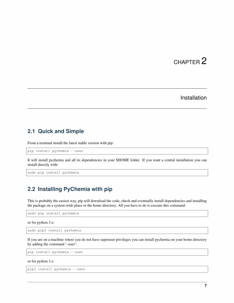
2.1 Quick and Simple
From a terminal install the latest stable version with pip:
pip install pychemia --user
It will install pychemia and all its dependencies in your $HOME folder. If you want a central installation you caninstall directly with:
sudo pip install pychemia
2.2 Installing PyChemia with pip
This is probably the easiest way, pip will download the code, check and eventually install dependencies and installingthe package on a system-wide place or the home directory. All you have to do is execute this command:
sudo pip install pychemia
or for python 3.x:
sudo pip3 install pychemia
If you are on a machine where you do not have superuser privileges you can install pychemia on your home directoryby adding the command ‘–user’:
pip install pychemia --user
or for python 3.x:
pip3 install pychemia --user
7
pychemia Documentation, Release 0.1.2
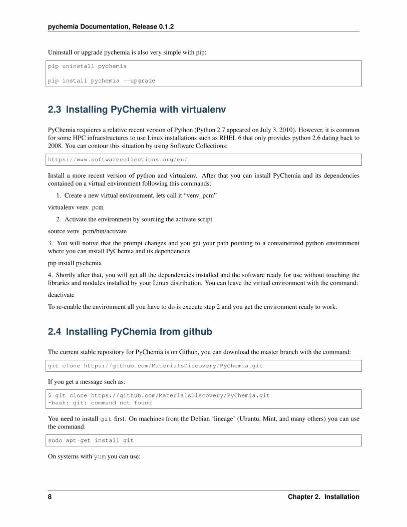
Uninstall or upgrade pychemia is also very simple with pip:
pip uninstall pychemia
pip install pychemia --upgrade
2.3 Installing PyChemia with virtualenv
PyChemia requieres a relative recent version of Python (Python 2.7 appeared on July 3, 2010). However, it is commonfor some HPC infraestructures to use Linux installations such as RHEL 6 that only provides python 2.6 dating back to2008. You can contour this situation by using Software Collections:
https://www.softwarecollections.org/en/
Install a more recent version of python and virtualenv. After that you can install PyChemia and its dependenciescontained on a virtual environment following this commands:
1. Create a new virtual environment, lets call it “venv_pcm”
virtualenv venv_pcm
2. Activate the environment by sourcing the activate script
source venv_pcm/bin/activate
3. You will notive that the prompt changes and you get your path pointing to a containerized python environmentwhere you can install PyChemia and its dependencies
pip install pychemia
4. Shortly after that, you will get all the dependencies installed and the software ready for use without touching thelibraries and modules installed by your Linux distribution. You can leave the virtual environment with the command:
deactivate
To re-enable the environment all you have to do is execute step 2 and you get the environment ready to work.
2.4 Installing PyChemia from github
The current stable repository for PyChemia is on Github, you can download the master branch with the command:
git clone https://github.com/MaterialsDiscovery/PyChemia.git
If you get a message such as:
$ git clone https://github.com/MaterialsDiscovery/PyChemia.git-bash: git: command not found
You need to install git first. On machines from the Debian ‘lineage’ (Ubuntu, Mint, and many others) you can usethe command:
sudo apt-get install git
On systems with yum you can use:
8 Chapter 2. Installation
pychemia Documentation, Release 0.1.2
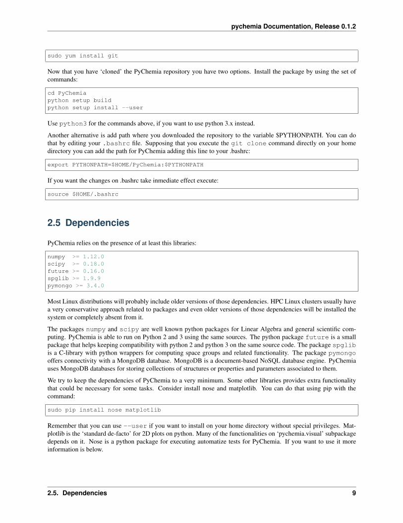
sudo yum install git
Now that you have ‘cloned’ the PyChemia repository you have two options. Install the package by using the set ofcommands:
cd PyChemiapython setup buildpython setup install --user
Use python3 for the commands above, if you want to use python 3.x instead.
Another alternative is add path where you downloaded the repository to the variable $PYTHONPATH. You can dothat by editing your .bashrc file. Supposing that you execute the git clone command directly on your homedirectory you can add the path for PyChemia adding this line to your .bashrc:
export PYTHONPATH=$HOME/PyChemia:$PYTHONPATH
If you want the changes on .bashrc take inmediate effect execute:
source $HOME/.bashrc
2.5 Dependencies
PyChemia relies on the presence of at least this libraries:
numpy >= 1.12.0scipy >= 0.18.0future >= 0.16.0spglib >= 1.9.9pymongo >= 3.4.0
Most Linux distributions will probably include older versions of those dependencies. HPC Linux clusters usually havea very conservative approach related to packages and even older versions of those dependencies will be installed thesystem or completely absent from it.
The packages numpy and scipy are well known python packages for Linear Algebra and general scientific com-puting. PyChemia is able to run on Python 2 and 3 using the same sources. The python package future is a smallpackage that helps keeping compatibility with python 2 and python 3 on the same source code. The package spglibis a C-library with python wrappers for computing space groups and related functionality. The package pymongooffers connectivity with a MongoDB database. MongoDB is a document-based NoSQL database engine. PyChemiauses MongoDB databases for storing collections of structures or properties and parameters associated to them.
We try to keep the dependencies of PyChemia to a very minimum. Some other libraries provides extra functionalitythat could be necessary for some tasks. Consider install nose and matplotlib. You can do that using pip with thecommand:
sudo pip install nose matplotlib
Remember that you can use --user if you want to install on your home directory without special privileges. Mat-plotlib is the ‘standard de-facto’ for 2D plots on python. Many of the functionalities on ‘pychemia.visual’ subpackagedepends on it. Nose is a python package for executing automatize tests for PyChemia. If you want to use it moreinformation is below.
2.5. Dependencies 9
pychemia Documentation, Release 0.1.2
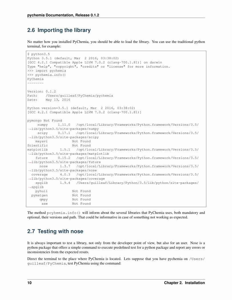
2.6 Importing the library
No matter how you installed PyChemia, you should be able to load the library. You can use the traditional pythonterminal, for example:
$ python3.5Python 3.5.1 (default, Mar 2 2016, 03:38:02)[GCC 4.2.1 Compatible Apple LLVM 7.0.2 (clang-700.1.81)] on darwinType "help", "copyright", "credits" or "license" for more information.>>> import pychemia>>> pychemia.info()PyChemia--------
Version: 0.1.2Path: /Users/guilleaf/PyChemia/pychemiaDate: May 13, 2016
Python version=3.5.1 (default, Mar 2 2016, 03:38:02)[GCC 4.2.1 Compatible Apple LLVM 7.0.2 (clang-700.1.81)]
pymongo Not Foundnumpy 1.11.0 /opt/local/Library/Frameworks/Python.framework/Versions/3.5/
→˓lib/python3.5/site-packages/numpyscipy 0.17.1 /opt/local/Library/Frameworks/Python.framework/Versions/3.5/
→˓lib/python3.5/site-packages/scipymayavi Not Found
Scientific Not Foundmatplotlib 1.5.1 /opt/local/Library/Frameworks/Python.framework/Versions/3.5/→˓lib/python3.5/site-packages/matplotlib
future 0.15.2 /opt/local/Library/Frameworks/Python.framework/Versions/3.5/→˓lib/python3.5/site-packages/future
nose 1.3.7 /opt/local/Library/Frameworks/Python.framework/Versions/3.5/→˓lib/python3.5/site-packages/nosecoverage 4.0.3 /opt/local/Library/Frameworks/Python.framework/Versions/3.5/
→˓lib/python3.5/site-packages/coveragespglib 1.9.4 /Users/guilleaf/Library/Python/3.5/lib/python/site-packages/
→˓spglibpyhull Not Found
pymatgen Not Foundqmpy Not Foundase Not Found
The method pcyhemia.info() will inform about the several libraries that PyChemia uses, both mandatory andoptional, their versions and path. That could be informative in case of something not working as expected.
2.7 Testing with nose
It is always important to test a library, not only from the developer point of view, but also for an user. Nose is apython package that offers a simple command to execute predefined test for a python package and report any errors orinconsistencies from the expected resuts.
Direct the terminal to the place where PyChemia is located. Lets suppose that you have pychemia on /Users/guilleaf/PyChemia, test PyChemia using the command:
10 Chapter 2. Installation
pychemia Documentation, Release 0.1.2
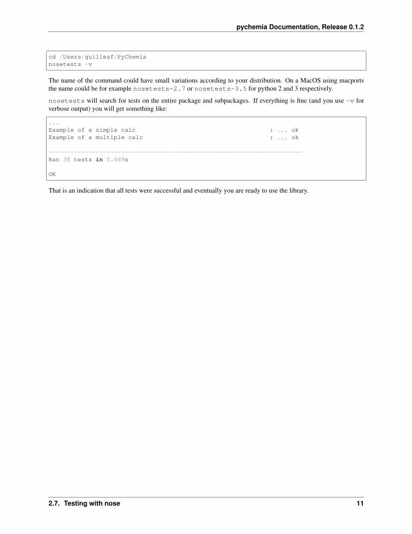
cd /Users/guilleaf/PyChemianosetests -v
The name of the command could have small variations according to your distribution. On a MacOS using macportsthe name could be for example nosetests-2.7 or nosetests-3.5 for python 2 and 3 respectively.
nosetests will search for tests on the entire package and subpackages. If everything is fine (and you use -v forverbose output) you will get something like:
...Example of a simple calc : ... okExample of a multiple calc : ... ok
----------------------------------------------------------------------Ran 38 tests in 5.469s
OK
That is an indication that all tests were successful and eventually you are ready to use the library.
2.7. Testing with nose 11
pychemia Documentation, Release 0.1.2
12 Chapter 2. Installation
CHAPTER 3
Quick Start
PyChemia is built from several layers of code, the foundations being the ability to manipulate conglomerates of atoms,either molecules or crystals. Before doing more complex operations such execute tasks on various electronic structurecodes or running structural searches we need to understand how the fundamental blocks work and that is the purposeof this quick start section.
For the examples presented here you can use the official python terminal, however, the IPython terminal or a Jupyternotebook offers you more power to go across the examples and explore what PyChemia can do for you. At least,installing IPython is very simple on many operating systems.
For example on machines running a debian derivative (Ubuntu, Mint and several others) you can use the followingcommand to install the IPython terminal:
sudo apt-get install python-ipython
or for python 3.x:
sudo apt-get install python3-python
On MacOS using macports:
sudo port install py27-ipython
or for python 3.x:
sudo port install py35-ipython
3.1 Element
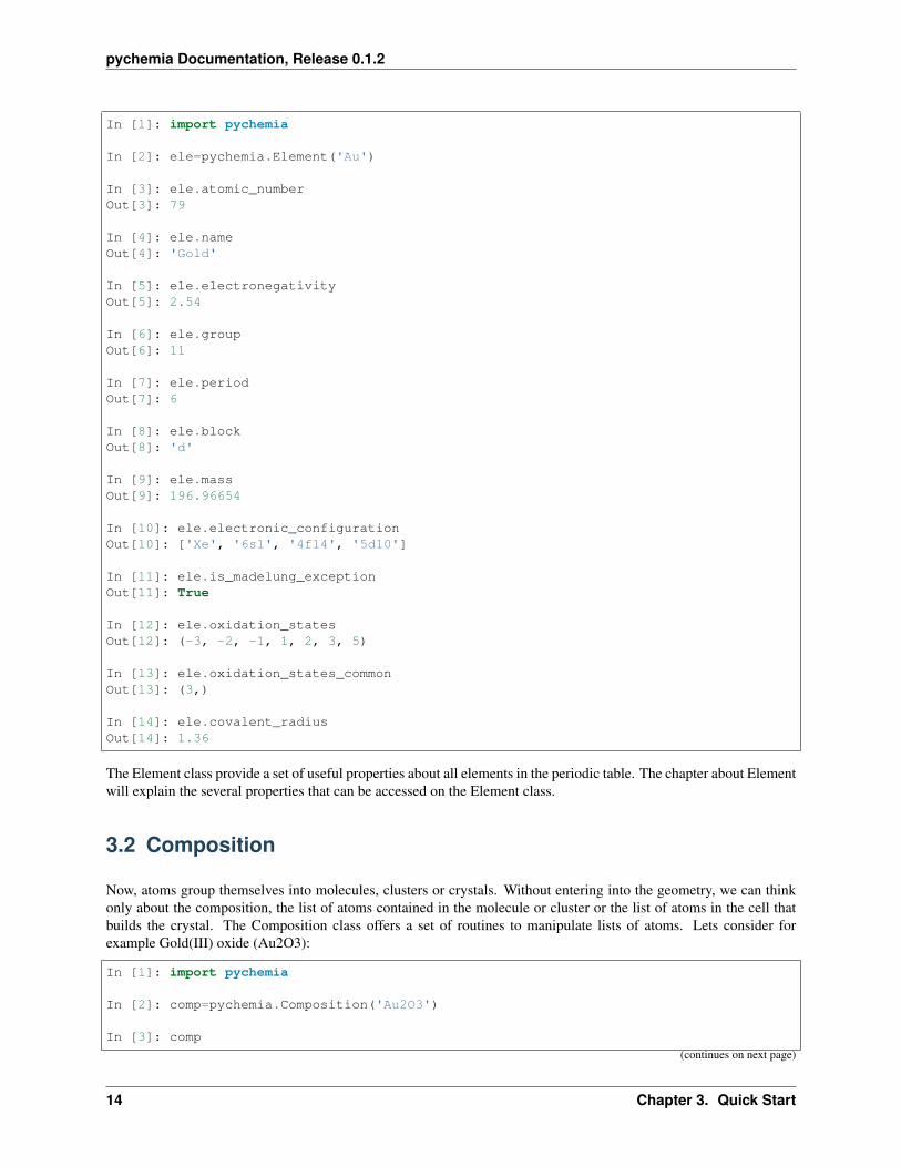
PyChemia is about materials, molecules, cluster and crystals. A class for elements can become handy to serve as aperiodic table and inquire for the properties of a given specie. Alchemy was all about transmuting materials into gold.Lets explore what PyChemia can tell us about that element:
13
pychemia Documentation, Release 0.1.2
In [1]: import pychemia
In [2]: ele=pychemia.Element('Au')
In [3]: ele.atomic_numberOut[3]: 79
In [4]: ele.nameOut[4]: 'Gold'
In [5]: ele.electronegativityOut[5]: 2.54
In [6]: ele.groupOut[6]: 11
In [7]: ele.periodOut[7]: 6
In [8]: ele.blockOut[8]: 'd'
In [9]: ele.massOut[9]: 196.96654
In [10]: ele.electronic_configurationOut[10]: ['Xe', '6s1', '4f14', '5d10']
In [11]: ele.is_madelung_exceptionOut[11]: True
In [12]: ele.oxidation_statesOut[12]: (-3, -2, -1, 1, 2, 3, 5)
In [13]: ele.oxidation_states_commonOut[13]: (3,)
In [14]: ele.covalent_radiusOut[14]: 1.36
The Element class provide a set of useful properties about all elements in the periodic table. The chapter about Elementwill explain the several properties that can be accessed on the Element class.
3.2 Composition
Now, atoms group themselves into molecules, clusters or crystals. Without entering into the geometry, we can thinkonly about the composition, the list of atoms contained in the molecule or cluster or the list of atoms in the cell thatbuilds the crystal. The Composition class offers a set of routines to manipulate lists of atoms. Lets consider forexample Gold(III) oxide (Au2O3):
In [1]: import pychemia
In [2]: comp=pychemia.Composition('Au2O3')
In [3]: comp
(continues on next page)
14 Chapter 3. Quick Start
pychemia Documentation, Release 0.1.2
(continued from previous page)
Out[3]: Composition({'Au': 2, 'O': 3})
In [4]: comp['Au']Out[4]: 2
In [5]: comp.nspeciesOut[5]: 2
In [6]: comp.symbolsOut[6]: ['Au', 'Au', 'O', 'O', 'O']
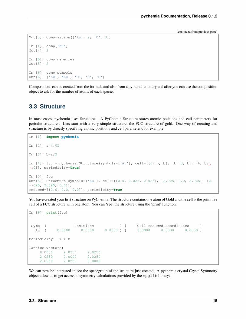
Compositions can be created from the formula and also from a python dictionary and after you can use the compositionobject to ask for the number of atoms of each specie.
3.3 Structure
In most cases, pychemia uses Structures. A PyChemia Structure stores atomic positions and cell parameters forperiodic structures. Lets start with a very simple structure, the FCC structure of gold. One way of creating andstructure is by directly specifying atomic positions and cell parameters, for example:
In [1]: import pychemia
In [2]: a=4.05
In [3]: b=a/2
In [4]: fcc = pychemia.Structure(symbols=['Au'], cell=[[0, b, b], [b, 0, b], [b, b,→˓0]], periodicity=True)
In [5]: fccOut[5]: Structure(symbols=['Au'], cell=[[0.0, 2.025, 2.025], [2.025, 0.0, 2.025], [2.→˓025, 2.025, 0.0]],reduced=[[0.0, 0.0, 0.0]], periodicity=True)
You have created your first structure on PyChemia. The structure contains one atom of Gold and the cell is the primitivecell of a FCC structure with one atom. You can ‘see’ the structure using the ‘print’ function:
In [6]: print(fcc)1
Symb ( Positions ) [ Cell-reduced coordinates ]Au ( 0.0000 0.0000 0.0000 ) [ 0.0000 0.0000 0.0000 ]
Periodicity: X Y Z
Lattice vectors:0.0000 2.0250 2.02502.0250 0.0000 2.02502.0250 2.0250 0.0000
We can now be interested in see the spacegroup of the structure just created. A pychemia.crystal.CrystalSymmetryobject allow us to get access to symmetry calculations provided by the spglib library:
3.3. Structure 15
pychemia Documentation, Release 0.1.2
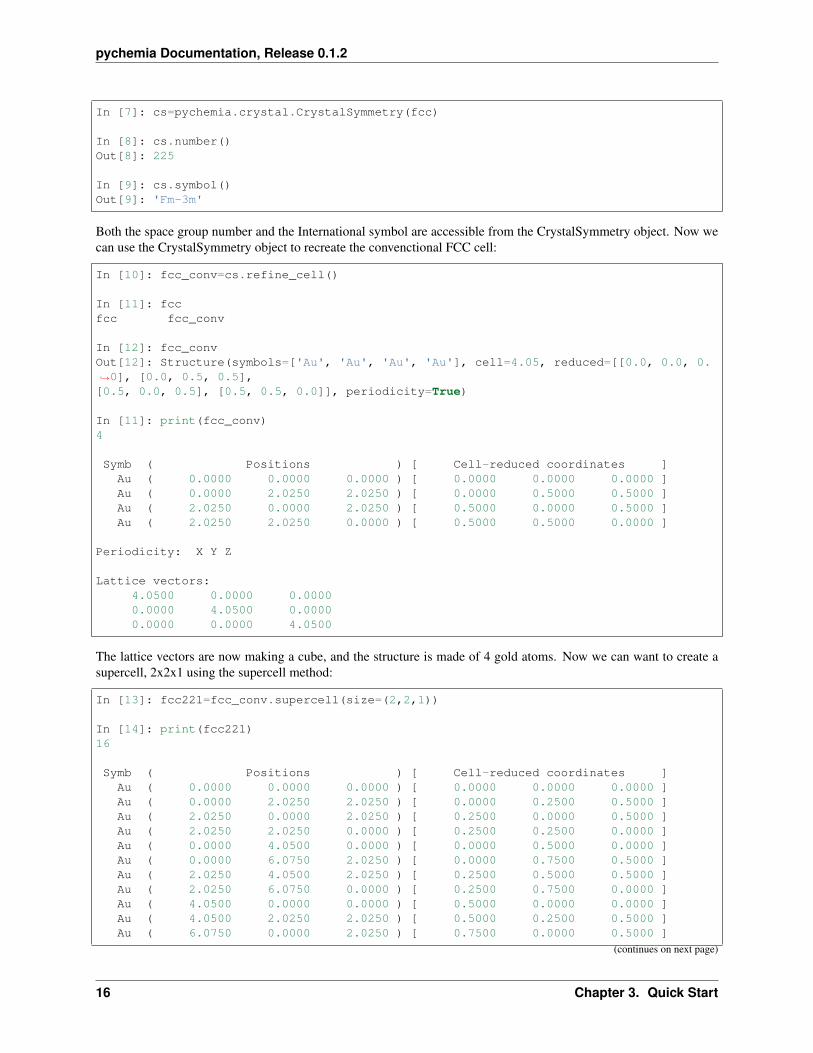
In [7]: cs=pychemia.crystal.CrystalSymmetry(fcc)
In [8]: cs.number()Out[8]: 225
In [9]: cs.symbol()Out[9]: 'Fm-3m'
Both the space group number and the International symbol are accessible from the CrystalSymmetry object. Now wecan use the CrystalSymmetry object to recreate the convenctional FCC cell:
In [10]: fcc_conv=cs.refine_cell()
In [11]: fccfcc fcc_conv
In [12]: fcc_convOut[12]: Structure(symbols=['Au', 'Au', 'Au', 'Au'], cell=4.05, reduced=[[0.0, 0.0, 0.→˓0], [0.0, 0.5, 0.5],[0.5, 0.0, 0.5], [0.5, 0.5, 0.0]], periodicity=True)
In [11]: print(fcc_conv)4
Symb ( Positions ) [ Cell-reduced coordinates ]Au ( 0.0000 0.0000 0.0000 ) [ 0.0000 0.0000 0.0000 ]Au ( 0.0000 2.0250 2.0250 ) [ 0.0000 0.5000 0.5000 ]Au ( 2.0250 0.0000 2.0250 ) [ 0.5000 0.0000 0.5000 ]Au ( 2.0250 2.0250 0.0000 ) [ 0.5000 0.5000 0.0000 ]
Periodicity: X Y Z
Lattice vectors:4.0500 0.0000 0.00000.0000 4.0500 0.00000.0000 0.0000 4.0500
The lattice vectors are now making a cube, and the structure is made of 4 gold atoms. Now we can want to create asupercell, 2x2x1 using the supercell method:
In [13]: fcc221=fcc_conv.supercell(size=(2,2,1))
In [14]: print(fcc221)16
Symb ( Positions ) [ Cell-reduced coordinates ]Au ( 0.0000 0.0000 0.0000 ) [ 0.0000 0.0000 0.0000 ]Au ( 0.0000 2.0250 2.0250 ) [ 0.0000 0.2500 0.5000 ]Au ( 2.0250 0.0000 2.0250 ) [ 0.2500 0.0000 0.5000 ]Au ( 2.0250 2.0250 0.0000 ) [ 0.2500 0.2500 0.0000 ]Au ( 0.0000 4.0500 0.0000 ) [ 0.0000 0.5000 0.0000 ]Au ( 0.0000 6.0750 2.0250 ) [ 0.0000 0.7500 0.5000 ]Au ( 2.0250 4.0500 2.0250 ) [ 0.2500 0.5000 0.5000 ]Au ( 2.0250 6.0750 0.0000 ) [ 0.2500 0.7500 0.0000 ]Au ( 4.0500 0.0000 0.0000 ) [ 0.5000 0.0000 0.0000 ]Au ( 4.0500 2.0250 2.0250 ) [ 0.5000 0.2500 0.5000 ]Au ( 6.0750 0.0000 2.0250 ) [ 0.7500 0.0000 0.5000 ]
(continues on next page)
16 Chapter 3. Quick Start
pychemia Documentation, Release 0.1.2
(continued from previous page)
Au ( 6.0750 2.0250 0.0000 ) [ 0.7500 0.2500 0.0000 ]Au ( 4.0500 4.0500 0.0000 ) [ 0.5000 0.5000 0.0000 ]Au ( 4.0500 6.0750 2.0250 ) [ 0.5000 0.7500 0.5000 ]Au ( 6.0750 4.0500 2.0250 ) [ 0.7500 0.5000 0.5000 ]Au ( 6.0750 6.0750 0.0000 ) [ 0.7500 0.7500 0.0000 ]
Periodicity: X Y Z
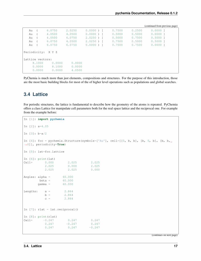
Lattice vectors:8.1000 0.0000 0.00000.0000 8.1000 0.00000.0000 0.0000 4.0500
PyChemia is much more than just elements, compositions and structures. For the purpose of this introduction, thoseare the most basic building blocks for most of the of higher level operations such as populations and global searches.
3.4 Lattice
For periodic structures, the lattice is fundamental to describe how the geometry of the atoms is repeated. PyChemiaoffers a class Lattice for manipulate cell parameters both for the real space lattice and the reciprocal one. For examplefrom the example before:
In [1]: import pychemia
In [2]: a=4.05
In [3]: b=a/2
In [4]: fcc = pychemia.Structure(symbols=['Au'], cell=[[0, b, b], [b, 0, b], [b, b,→˓0]], periodicity=True)
In [5]: lat=fcc.lattice
In [6]: print(lat)Cell= 0.000 2.025 2.025
2.025 0.000 2.0252.025 2.025 0.000
Angles: alpha = 60.000beta = 60.000gamma = 60.000
Lengths: a = 2.864b = 2.864c = 2.864
In [7]: rlat = lat.reciprocal()
In [8]: print(rlat)Cell= -0.247 0.247 0.247
0.247 -0.247 0.2470.247 0.247 -0.247
(continues on next page)
3.4. Lattice 17
pychemia Documentation, Release 0.1.2
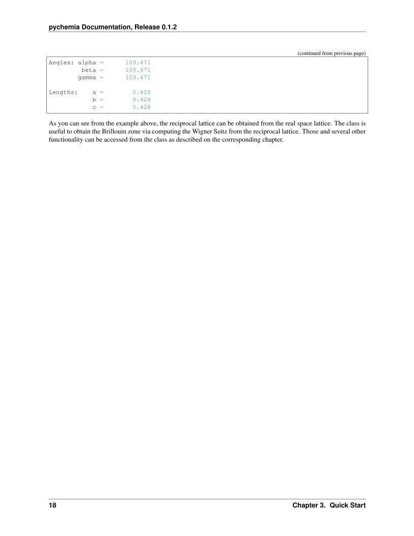
(continued from previous page)
Angles: alpha = 109.471beta = 109.471gamma = 109.471
Lengths: a = 0.428b = 0.428c = 0.428
As you can see from the example above, the reciprocal lattice can be obtained from the real space lattice. The class isuseful to obtain the Brillouin zone via computing the Wigner Seitz from the reciprocal lattice. Those and several otherfunctionality can be accessed from the class as described on the corresponding chapter.
18 Chapter 3. Quick Start

CHAPTER 4
Global Minimization with Metaheuristics
One of the first features implemented on PyChemia was the ability to perform global minimization for various purposesin materials science using a variety of Metaheuristic algorithms. On this set of tutorials, we will demonstrate thiscapability in a variety of problems: Searching optimal configurations of Lennard-Jones clusters, finding structures ofbinaries and ternaries using several Tight-Binding and DFT codes, optimizing the Magnetic Moments with VASP andoptimizing the density matrices for DFT+U using ABINIT.
4.1 Global Minimimization of Lennard-Jones Clusters
This tutorial will guide to how search for global minima using the methods implemented on PyChemia.
4.1.1 Quick version
The shortest version of a global search using the FireFly method will look like this
>>> from pychemia.searcher import FireFly>>> from pychemia.population import LJCluster>>> popu = LJCluster('LJ13', composition='Xe13', refine=True, direct_evaluation=True)>>> searcher = FireFly(popu, generation_size=16, stabilization_limit=10)>>> searcher.run()
For this case, you should have a mongo server running on you local machine, no SSL encryption and no authorizationwith username and password. The population will be created with Lennard-Jones clusters with 13 particles each. Eachnew candidate is locally relaxed when created. The searcher will use 16 candidates on each generation and will stopwhen the best candidate survives for 10 generations.
4.2 PyChemia Software Framework
PyChemia is framework for materials discovery, more than just compute DFT calculations for structures alreadypresent in databases such as ICSD, PyChemia searches for new structures that could never have been synthesized or
19
pychemia Documentation, Release 0.1.2
reported before.
To achieve its goal, PyChemia relies on a number of methods of structural search such as minima hoping method,genetic algorithms and other population based algorithms.
As a software framework, PyChemia is structurated around five axis. They are:
1. Structural Search Methods
2. Storage and Databases
3. Data Mining or Knowledge Discovery in Data
4. Execution and Analysis
5. Reporting and Visualization
We will develop those five axis and the relations between them
4.2.1 Structural Search Methods
One of the distinctive characteristics of PyChemia is its ability to search for new structures. Ab-initio calculations ofstructures present of databases such as ICSD becomes limited to the extension of the original databases. Even if sucheffort is indeed a big challenge with large databases, those databases represent a small portion of the structures thatcould be created. The ability to predict new structures and target those findings to specific applications is a task oftechnological relevance.
PyChemia was created with an strong focus on structural prediction. PyChemia implements several methods, fromminima hoping method to metaheuristics
4.2.1.1 Minima Hoping Method
4.2.1.2 Metaheuristics
4.2.2 Storage and Databases
If PyChemia were a software to compute ab-initio calculations from structures taken from another database or fromvery predictive set of prototypes only one database will be enough. However, as we mention before PyChemia isfocused on structural search.
The kind of algorithms that we describe above typically explore thousands of different structures before selecting areduced subset of thermodynamically stable or metastable ones.
Also, the search for new structures must be guided by specific applications of interest, batteries, thermoelectrics,superconductors, etc. Different applications are associated to different properties in the electronic structure.
Those two elements, the dynamic nature of structural search methods and the flexibility in the data that we would liketo store is the reason why we are not using a single database and why we departed from traditional SQL schemas.
PyChemia was designed to create new databases for each structural search. We still keep one large database witha curated selection of structures but the ability to create small and flexible databases is central for the success ofPyChemia.
PyChemia relies on MongoDB. MongoDB is an open-source document database, and the leading NoSQL database.We take advantage of dynamic schemas that offer simplicity and power and are in harmony with the own principles ofscientific research. Different structures are intended for different applications and different applications requieres thecalculation of different physical properties.
20 Chapter 4. Global Minimization with Metaheuristics
pychemia Documentation, Release 0.1.2
4.2.3 Data Mining or Knowledge Discovery in Data
Data Mining or more correctly Knowledge Discovery in Data is the computational process of discovering patterns inlarge data sets involving methods at the intersection of artificial intelligence, machine learning, statistics, and databasesystems.
Structural Search algorithms has the ability to gererate in the long term more structures that those that could be syn-thesized in reasonable time. As the database becomes large traditional techniques based on estimate good candidatesbased on just a few properties will be replaced by automatize algorithms that search patterns in structures and predictwere new stochiometries deserve exploration.
4.2.3.1 Bayesian networks and Gaussian Processes
4.2.4 Reporting and Visualization
Doing electronic structure calculations for thousands of materials is challenging but there is not point in doing thatwithout the ability to communicate to experimentalist structures that worth to be synthesized. PyChemia uses Djangoas a web-frontend to display and explore the computations not only on the global database but also on the specificdatabase product of a structural search run.
4.2.5 Execution and Analysis
There are two levels of execution in structural search runs. Ab-initio calculations and structural analysis. PyChemiaprovides concurrent execution and basic job management for running multiple ab-initio calculations on clusters ornon-queue systems
PyChemia relies on state-of-the-art ab-initio software packages to compute electronic structure and their properties.In particular PyChemia has support for VASP, ABINIT, Octopus, Fireball and DFTB+
Different levels of theory allows for a better compromise between accuracy and computational cost.
Structural analysis is defined as all kinds of procedures that relies only on structural data, for example structuralfingerprints, topological analysis, hardness calculations, comparators and symmetry calculations. PyChemia providesmulti-threaded execution of structural analysis routines
4.3 Optimization of Magnetic Moments (VASP)
This tutorial shows how to perform global search for optimal magnetic moments on VASP.
In VASP there are two variables that control the magnetic moments imposed on atoms and for contrain magneticmoments along predefined directions.
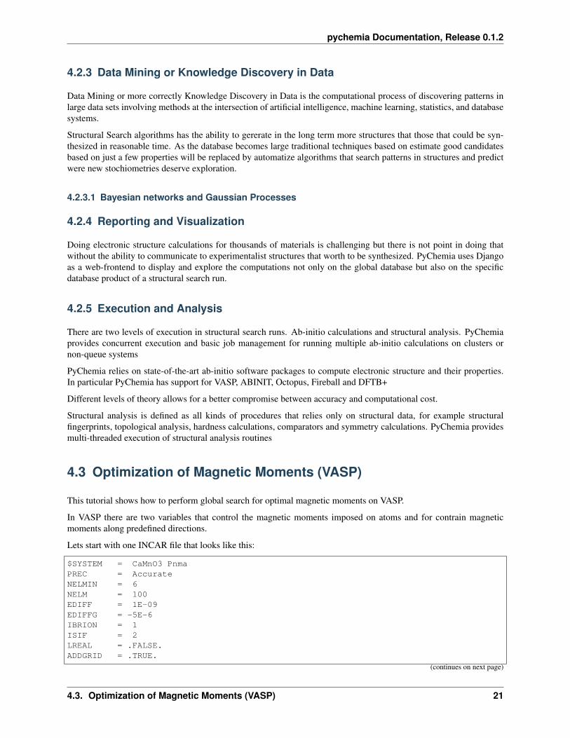
Lets start with one INCAR file that looks like this:
$SYSTEM = CaMnO3 PnmaPREC = AccurateNELMIN = 6NELM = 100EDIFF = 1E-09EDIFFG = -5E-6IBRION = 1ISIF = 2LREAL = .FALSE.ADDGRID = .TRUE.
(continues on next page)
4.3. Optimization of Magnetic Moments (VASP) 21
pychemia Documentation, Release 0.1.2
(continued from previous page)
NSW = 0ISMEAR = -5ENCUT = 500ISPIN = 2LORBIT = 11LMAXMIX = 4ISYM = 0LSORBIT = .TRUE.RWIGS = 2.00 1.87 1.78 1.24 # d-d/2SAXIS = 0 0 1LPLANE = .TRUE.NPAR = 2LSCALU = .FALSE.NSIM = 4LWAVE = .FALSE.AMIX = 0.8BMIX = 0.9AMIX_MAG = 0.4BMIX_MAG = 0.9
MAGMOM = 12*00.0000000 0.0416472 2.38596770.0000000 0.0416472 -2.38596770.0000000 0.0416472 -2.38596770.0000000 0.0416472 2.385967760*0
M_CONSTR = 12*00.0000000 0.0416472 2.38596770.0000000 0.0416472 -2.38596770.0000000 0.0416472 -2.38596770.0000000 0.0416472 2.385967760*0
I_CONSTRAINED_M = 1LAMBDA = 10
#LDAU = .TRUE.#LDAUTYPE = 1#LDAUL = -1 2 -1#LDAUU = 0.0 4.0 0.0#LDAUJ = 0.0 0.0 0.0#LDAUPRINT = 2
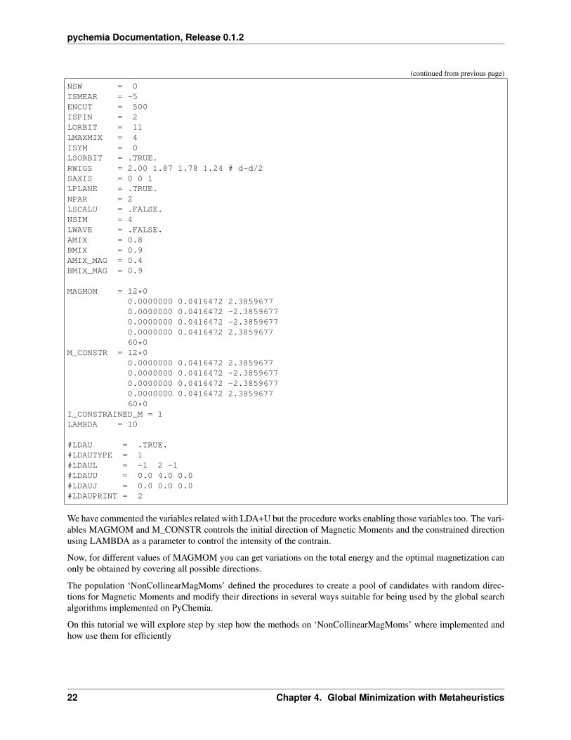
We have commented the variables related with LDA+U but the procedure works enabling those variables too. The vari-ables MAGMOM and M_CONSTR controls the initial direction of Magnetic Moments and the constrained directionusing LAMBDA as a parameter to control the intensity of the contrain.
Now, for different values of MAGMOM you can get variations on the total energy and the optimal magnetization canonly be obtained by covering all possible directions.
The population ‘NonCollinearMagMoms’ defined the procedures to create a pool of candidates with random direc-tions for Magnetic Moments and modify their directions in several ways suitable for being used by the global searchalgorithms implemented on PyChemia.
On this tutorial we will explore step by step how the methods on ‘NonCollinearMagMoms’ where implemented andhow use them for efficiently
22 Chapter 4. Global Minimization with Metaheuristics
pychemia Documentation, Release 0.1.2
4.4 Global optimization of correlation matrices for DFT+U (Abinit)
4.4.1 The variable dmatpawu
The objective of this global search is finding the optimal values for the density matrices in DFT+U. ABINIT allowsto locally optimize the density matrices from a given initial value. The initial density matrices used in LDA+U arekept fixed during the first usedmatpu SCF iterations. For SCF iterations beyond that, the density matrices change. Thechallenge here is that from a given initial set of density matrices the system gets easily trapped into a local minimun,the usual procedure then is to start from several initial options hoping to reach the global minimum at some point.
A global minimizer takes the responsability of efficiently explore the configuration space of the problem. PyChemiaimplements several global searchers as we saw on previous tutorials. Those global searchers joined by an efficientevaluation infraestructure allows many evaluations being perform without human assistance and an effective chanceof reaching a global minimum if the search is long enough.
For this tutorial consider the following problem:
‘pychemia/test/data/abinit_dmatpaw/abinit.in’.
First, we can read the abinit input and access the contents of the variable ‘dmatpawu’:
import pychemiaimport numpy as nppychemia_path = pychemia.__path__[0]abiinput = pychemia.code.abinit.InputVariables(pychemia_path + '/test/data/abinit_→˓dmatpawu/abinit.in')dmatpawu = np.array(abiinput['dmatpawu']).reshape(-1,5,5)
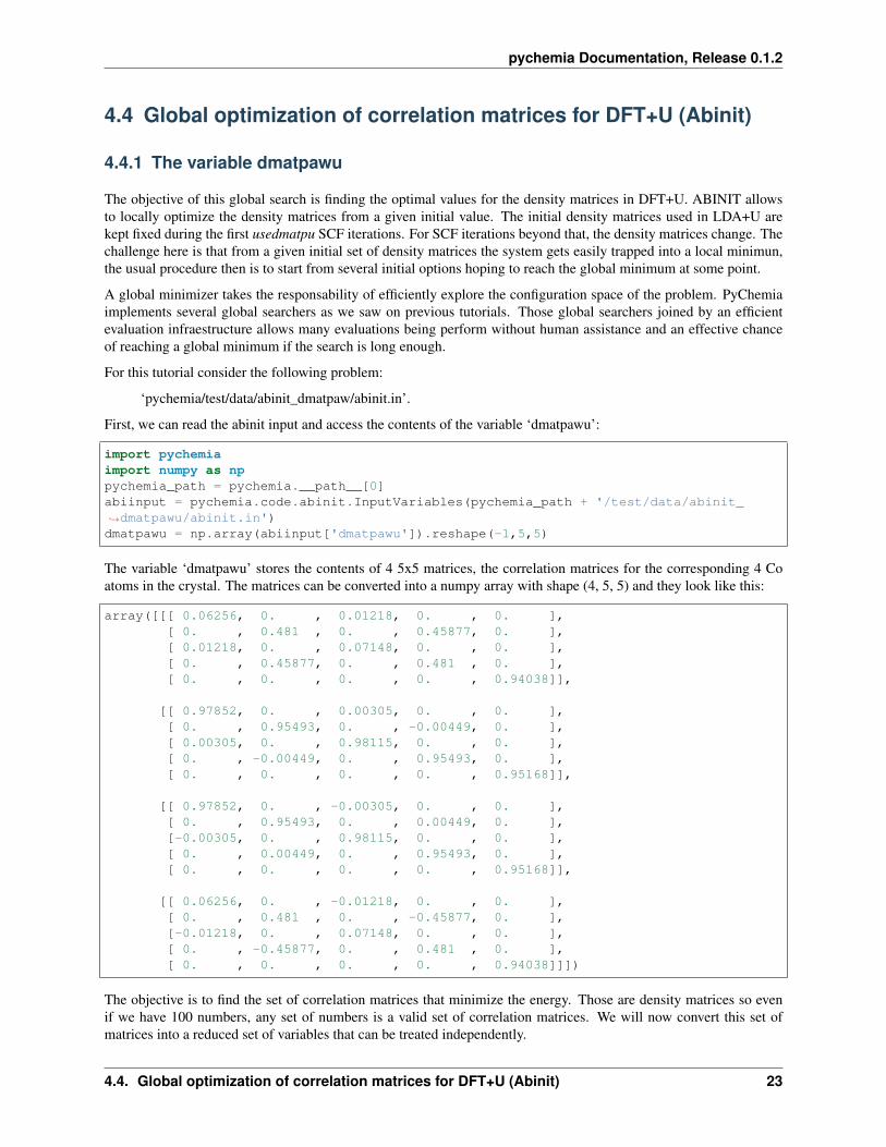
The variable ‘dmatpawu’ stores the contents of 4 5x5 matrices, the correlation matrices for the corresponding 4 Coatoms in the crystal. The matrices can be converted into a numpy array with shape (4, 5, 5) and they look like this:
array([[[ 0.06256, 0. , 0.01218, 0. , 0. ],[ 0. , 0.481 , 0. , 0.45877, 0. ],[ 0.01218, 0. , 0.07148, 0. , 0. ],[ 0. , 0.45877, 0. , 0.481 , 0. ],[ 0. , 0. , 0. , 0. , 0.94038]],
[[ 0.97852, 0. , 0.00305, 0. , 0. ],[ 0. , 0.95493, 0. , -0.00449, 0. ],[ 0.00305, 0. , 0.98115, 0. , 0. ],[ 0. , -0.00449, 0. , 0.95493, 0. ],[ 0. , 0. , 0. , 0. , 0.95168]],
[[ 0.97852, 0. , -0.00305, 0. , 0. ],[ 0. , 0.95493, 0. , 0.00449, 0. ],[-0.00305, 0. , 0.98115, 0. , 0. ],[ 0. , 0.00449, 0. , 0.95493, 0. ],[ 0. , 0. , 0. , 0. , 0.95168]],
[[ 0.06256, 0. , -0.01218, 0. , 0. ],[ 0. , 0.481 , 0. , -0.45877, 0. ],[-0.01218, 0. , 0.07148, 0. , 0. ],[ 0. , -0.45877, 0. , 0.481 , 0. ],[ 0. , 0. , 0. , 0. , 0.94038]]])
The objective is to find the set of correlation matrices that minimize the energy. Those are density matrices so evenif we have 100 numbers, any set of numbers is a valid set of correlation matrices. We will now convert this set ofmatrices into a reduced set of variables that can be treated independently.
4.4. Global optimization of correlation matrices for DFT+U (Abinit) 23
pychemia Documentation, Release 0.1.2
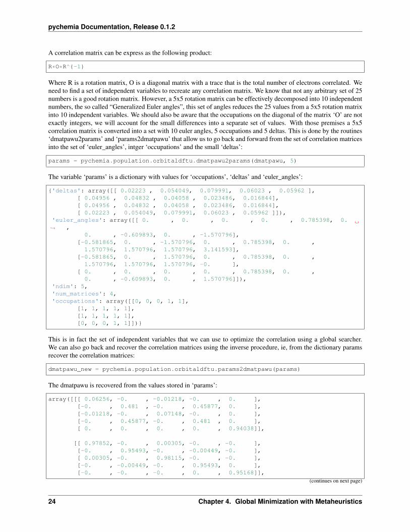
A correlation matrix can be express as the following product:
R*O*R^{-1}
Where R is a rotation matrix, O is a diagonal matrix with a trace that is the total number of electrons correlated. Weneed to find a set of independent variables to recreate any correlation matrix. We know that not any arbitrary set of 25numbers is a good rotation matrix. However, a 5x5 rotation matrix can be effectively decomposed into 10 independentnumbers, the so called “Generalized Euler angles”, this set of angles reduces the 25 values from a 5x5 rotation matrixinto 10 independent variables. We should also be aware that the occupations on the diagonal of the matrix ‘O’ are notexactly integers, we will account for the small differences into a separate set of values. With those premises a 5x5correlation matrix is converted into a set with 10 euler angles, 5 occupations and 5 deltas. This is done by the routines‘dmatpawu2params’ and ‘params2dmatpawu’ that allow us to go back and forward from the set of correlation matricesinto the set of ‘euler_angles’, intger ‘occupations’ and the small ‘deltas’:
params = pychemia.population.orbitaldftu.dmatpawu2params(dmatpawu, 5)
The variable ‘params’ is a dictionary with values for ‘occupations’, ‘deltas’ and ‘euler_angles’:
{'deltas': array([[ 0.02223 , 0.054049, 0.079991, 0.06023 , 0.05962 ],[ 0.04956 , 0.04832 , 0.04058 , 0.023486, 0.016844],[ 0.04956 , 0.04832 , 0.04058 , 0.023486, 0.016844],[ 0.02223 , 0.054049, 0.079991, 0.06023 , 0.05962 ]]),
'euler_angles': array([[ 0. , 0. , 0. , 0. , 0.785398, 0.→˓ ,
0. , -0.609893, 0. , -1.570796],[-0.581865, 0. , -1.570796, 0. , 0.785398, 0. ,1.570796, 1.570796, 1.570796, 3.141593],
[-0.581865, 0. , 1.570796, 0. , 0.785398, 0. ,1.570796, 1.570796, 1.570796, -0. ],
[ 0. , 0. , 0. , 0. , 0.785398, 0. ,0. , -0.609893, 0. , 1.570796]]),
'ndim': 5,'num_matrices': 4,'occupations': array([[0, 0, 0, 1, 1],
[1, 1, 1, 1, 1],[1, 1, 1, 1, 1],[0, 0, 0, 1, 1]])}
This is in fact the set of independent variables that we can use to optimize the correlation using a global searcher.We can also go back and recover the correlation matrices using the inverse procedure, ie, from the dictionary paramsrecover the correlation matrices:
dmatpawu_new = pychemia.population.orbitaldftu.params2dmatpawu(params)
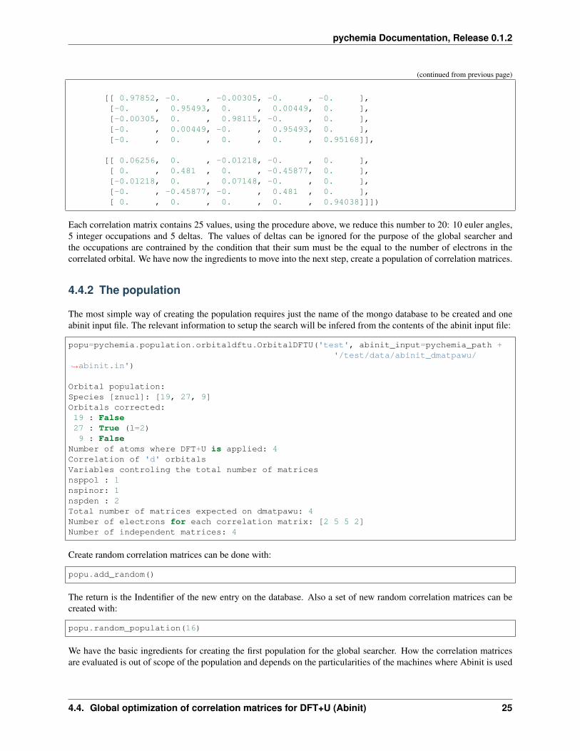
The dmatpawu is recovered from the values stored in ‘params’:
array([[[ 0.06256, -0. , -0.01218, -0. , 0. ],[-0. , 0.481 , -0. , 0.45877, 0. ],[-0.01218, -0. , 0.07148, -0. , 0. ],[-0. , 0.45877, -0. , 0.481 , 0. ],[ 0. , 0. , 0. , 0. , 0.94038]],
[[ 0.97852, -0. , 0.00305, -0. , -0. ],[-0. , 0.95493, -0. , -0.00449, -0. ],[ 0.00305, -0. , 0.98115, -0. , -0. ],[-0. , -0.00449, -0. , 0.95493, 0. ],[-0. , -0. , -0. , 0. , 0.95168]],
(continues on next page)
24 Chapter 4. Global Minimization with Metaheuristics
pychemia Documentation, Release 0.1.2
(continued from previous page)
[[ 0.97852, -0. , -0.00305, -0. , -0. ],[-0. , 0.95493, 0. , 0.00449, 0. ],[-0.00305, 0. , 0.98115, -0. , 0. ],[-0. , 0.00449, -0. , 0.95493, 0. ],[-0. , 0. , 0. , 0. , 0.95168]],
[[ 0.06256, 0. , -0.01218, -0. , 0. ],[ 0. , 0.481 , 0. , -0.45877, 0. ],[-0.01218, 0. , 0.07148, -0. , 0. ],[-0. , -0.45877, -0. , 0.481 , 0. ],[ 0. , 0. , 0. , 0. , 0.94038]]])
Each correlation matrix contains 25 values, using the procedure above, we reduce this number to 20: 10 euler angles,5 integer occupations and 5 deltas. The values of deltas can be ignored for the purpose of the global searcher andthe occupations are contrained by the condition that their sum must be the equal to the number of electrons in thecorrelated orbital. We have now the ingredients to move into the next step, create a population of correlation matrices.
4.4.2 The population
The most simple way of creating the population requires just the name of the mongo database to be created and oneabinit input file. The relevant information to setup the search will be infered from the contents of the abinit input file:
popu=pychemia.population.orbitaldftu.OrbitalDFTU('test', abinit_input=pychemia_path +'/test/data/abinit_dmatpawu/
→˓abinit.in')
Orbital population:Species [znucl]: [19, 27, 9]Orbitals corrected:19 : False27 : True (l=2)9 : False
Number of atoms where DFT+U is applied: 4Correlation of 'd' orbitalsVariables controling the total number of matricesnsppol : 1nspinor: 1nspden : 2Total number of matrices expected on dmatpawu: 4Number of electrons for each correlation matrix: [2 5 5 2]Number of independent matrices: 4
Create random correlation matrices can be done with:
popu.add_random()
The return is the Indentifier of the new entry on the database. Also a set of new random correlation matrices can becreated with:
popu.random_population(16)
We have the basic ingredients for creating the first population for the global searcher. How the correlation matricesare evaluated is out of scope of the population and depends on the particularities of the machines where Abinit is used
4.4. Global optimization of correlation matrices for DFT+U (Abinit) 25
pychemia Documentation, Release 0.1.2
to evaluate them. We will move our focus to the methods needed to produced new correlation matrices based on theresults of a given set of correlation matrices.
26 Chapter 4. Global Minimization with Metaheuristics
CHAPTER 5
Indices and tables
• genindex
• modindex
• search
27