Embed Size (px)
Citation preview
Relativistic Effects inAtomic Spectra
Diploma Thesisby
Robert Lang
Supervisor: Prof. Dr. Gero Friesecke
Submission Date: May 31, 2011
Technische Universitat Munchen
Fakultat fur Mathematik

Contents
1 Introduction 5
2 Spectrum of the Hydrogen Atom 72.1 Non-relativistic Schrodinger Model . . . . . . . . . . . . . . . . . . . . . . 7
2.1.1 Preliminaries . . . . . . . . . . . . . . . . . . . . . . . . . . . . . . 72.1.2 Weyl’s Criterion . . . . . . . . . . . . . . . . . . . . . . . . . . . . . 102.1.3 The Kato-Rellich Theorem . . . . . . . . . . . . . . . . . . . . . . . 122.1.4 Self-adjointness of the Hydrogen Hamiltonian . . . . . . . . . . . . 132.1.5 Non-relativistic Spectrum of the Hydrogen Atom . . . . . . . . . . 15
2.2 Relativistic Dirac Model . . . . . . . . . . . . . . . . . . . . . . . . . . . . 182.2.1 Self-adjointness of the Dirac Operator . . . . . . . . . . . . . . . . . 182.2.2 Dirac Operator with Coulomb Interaction . . . . . . . . . . . . . . 232.2.3 Non-relativistic Limit and its Relativistic Corrections . . . . . . . . 25
3 Spectrum of Many-electron Atoms 293.1 Non-relativistic Perturbation-theory Model . . . . . . . . . . . . . . . . . . 29
3.1.1 Definition of the PT Model . . . . . . . . . . . . . . . . . . . . . . 293.1.2 Principal Results . . . . . . . . . . . . . . . . . . . . . . . . . . . . 323.1.3 Energy Levels and Spectral Gaps . . . . . . . . . . . . . . . . . . . 34
3.2 Relativistic Effects in Asymptotic PT States . . . . . . . . . . . . . . . . . 383.2.1 P-contribution and Darwin Term . . . . . . . . . . . . . . . . . . . 383.2.2 Spin-orbit Coupling . . . . . . . . . . . . . . . . . . . . . . . . . . . 413.2.3 Relativistic Energy Levels, Spectral Gaps and Splitting . . . . . . . 44
3.3 Relativistic Corrections to Lithium . . . . . . . . . . . . . . . . . . . . . . 453.3.1 Shifted Energy Levels . . . . . . . . . . . . . . . . . . . . . . . . . . 453.3.2 Effective Nuclear Charge . . . . . . . . . . . . . . . . . . . . . . . . 48
3.4 Relativistic Corrections to Beryllium, Boron and Carbon . . . . . . . . . . 503.5 Relativistic Corrections to Nitrogen, Oxygen, Fluorine and Neon . . . . . . 573.6 Non-local Relativistic Corrections . . . . . . . . . . . . . . . . . . . . . . . 65
4 Summary and Conclusion 71
A Appendix 77A.1 Sobolev Spaces . . . . . . . . . . . . . . . . . . . . . . . . . . . . . . . . . 77A.2 Spherical Harmonics and Laguerre Polynomials . . . . . . . . . . . . . . . 79
A.2.1 Spherical Harmonics . . . . . . . . . . . . . . . . . . . . . . . . . . 79A.2.2 Laguerre Polynomials . . . . . . . . . . . . . . . . . . . . . . . . . . 82
A.3 Notations in Relativistic Quantum Mechanics . . . . . . . . . . . . . . . . 84
3

1 Introduction
Die Physik ist fur die Physiker eigentlich viel zu schwer.1
David Hilbert
The history of physics has shown an interesting progress of the comprehension of many-particle systems: in classical mechanics, the three-body problem has been known not beingsolvable generally. In electrodynamics, also the two-body case has become unsolvable.When quantum mechanics was emerging, new phenomena and paradoxes have occurredand one-particle systems needed to be discussed anew. Today, in quantum field theory orstring theory representing modern physics, we are not even sure about the vacuum.
In this thesis we investigate relativistic effects in atomic spectra, particularly the spec-tral gaps in many-electron atoms. We derive explicit perturbative results from first prin-ciples of quantum mechanics, the theory of special relativity and Dirac theory. The basiswe are working on is the non-relativistic perturbation-theory (PT) model, developed in[FG09b] and [FG10]. It provides asymptotic solutions for the eigenstates and eigenval-ues of the second-shell atoms Lithium to Neon. The key idea thereby is induced by theobservation that in many-electron atoms the electron-electron interaction is dominatedby the electron-nucleus interaction in the limit of large nuclear charges, Z → ∞, theso-called asymptotic limit. Therefore, the interaction between different electrons can betreated perturbatively for large Z. The asymptotic PT states are approximations of theSchrodinger eigenstates, but even in the case of neutral atoms their ground-state quantumnumbers coincide with those found in experiments. Comparisons of the asymptotic energygaps to experiments with highly-charged ions confirm the PT model. We use the NISTdatabase, [Yu.10], for the experimental data. We emphasize that the results obtainedwithin the PT model are independent of any semi-empirical input like Hund’s rules or theHartree-Fock method using a single Slater determinant of hydrogen orbitals as a startingpoint.
Of course, the experimental spectrum includes relativistic effects. These are not coveredby the PT model. The main goal of this thesis is the derivation and discussion of allfirst-order relativistic corrections to the energy levels of Lithium to Neon. The threecontributing corrections are well-known in the one-particle case: firstly, the relativisticenergy-momentum relation adjusts the classical kinetic energy. Secondly, retardationseffects due to a finite speed of light are represented by the Darwin term. Finally, thespin-orbit coupling incorporates the spin of the electrons. We show briefly how thesecorrections terms arise from the non-relativistic limit of Dirac theory. For the spin-orbitcoupling we restrict the main discussion to a local coupling between the spin of one electronand its angular momentum. Terms taking the spin and angular momentum of differentelectrons into account are assumed to be dominated by the local coupling. Our findingsconcerning the relativistically corrected energy gaps are compared to the experimentaldata from NIST. We will discuss the effects for each chemical element in detail.
1Actually, physics is too hard for physicists.
5
1 Introduction
This thesis is divided mainly into two parts: to begin with we need to understand thespectrum of the hydrogen atom as one-electron system.2 We introduce some fundamentalterms of spectral theory and prove the self-adjointness of the hydrogen Hamiltonian. Thehydrogen orbitals are essential for the PT model and its relativistic corrections, hencewe show in the Appendix a detailed derivation of them. We also introduce the Diracoperator and discuss its self-adjointness and its spectrum. From the Dirac operator allrelativistic correction terms can be derived by expanding its resolvent around the classicallimit point.
The second part of this thesis starts with the presentation of the PT model and itsprincipal results. Combining these with the correction terms obtained from Dirac theory,we derive in a general discussion all claimed relativistic corrections. In the subsequentdetailed discussion we specify the general corrections for all ground and first excited statesof Lithium, Beryllium, Boron, Carbon, Nitrogen, Oxygen and Fluorine. For Neon the PTmodel offers only the ground state which undergoes some relativistic shift but no splitting.
In particular we find theoretically that some spectral gaps for Lithium and Oxygenare not expected to feature relativistic corrections, since the relativistic corrections tothe involved energy levels are degenerate. This sort of degeneracy is well-known in theanalytically solvable hydrogen atom: there, the states 2s and 2p1/2 are degenerate in allorders of perturbation theory in the fine-structure constant α0. Indeed, the NIST datafeature the predicted degeneracies in the many-electron atoms, too.
Even the simplified local treatment of the spin-orbit coupling features the abolishmentof the mathematically indistinguishableness of the ground states of Boron and Fluorine,and Carbon and Oxygen. When taking only the quantum numbers L and S into accountthe ground states of the two considered pairs cannot be distinguished. The additionaltotal angular momentum, J , helps to label these ground states uniquely.
In this thesis we used JaxoDraw 2.0-1 to visualize the energy levels. The plots forthe spectral gaps and splittings were made using Microcal Origin 6.0.
2The electron-proton system features a small and large mass scale, m and M , respectively, hence it isusually considered as one-particle system. Due to a small reduced mass, µ ≡ mM/(m+M)→ m forlarge M , this approximation is feasible.
6
2 Spectrum of the Hydrogen Atom
2.1 Non-relativistic Schrodinger Model
A good definition should be the hypothesis of a theorem.James Glimm
This section is directed to understanding the non-relativistic spectrum of the hydrogenatom. The Schrodinger equation, Eψ = Hψ, describes the eigenvalues, E ∈ σp(H), ofthe hydrogen Hamiltonian H. We will investigate on which domain H is a self-adjointoperator and prepare the set of its eigenfunctions which are key ingredients for the PTmodel later on. We start with introducing some elementary definitions and theorems ofoperator theory and spectral theory.
2.1.1 Preliminaries
Definition 2.1. Let X and Y be two Hilbert spaces and D(A), called the domain of A,be a dense linear subspace of X. If the map A : D(A) → Y is linear, we call A a linearoperator in X and denote it by A : X → Y . A is called linear operator on X, ifD(A) = X. We call A a bounded linear operator, if
||A|| := sup|Ax| : x ∈ D(A), |x| = 1 <∞ . (2.1)
In this case the non-negative real number ||A|| is called the norm of the linear operatorA. We denote the set of all bounded linear operators on X by B(X,Y ); if X = Y wewrite briefly B(X). If A and B are linear operators in X, then A is said to be anextension of B, B ⊆ A, if D(B) ⊆ D(A) and Ax = Bx for all x ∈ D(B).
Definition 2.2. A linear operator A : X → Y is said to be closed if for all sequences(xn)n∈N ⊆ D(A) with xn → x ∈ D(A) and Axn → y ∈ Y , one has Ax = y.
Remark 2.3. In general, boundedness does not imply closeness. Furthermore, closenessdoes not imply boundedness. When restricting to operators A ∈ B(X, Y ), then, by theclosed graph theorem, A is bounded ⇔ A is closed.
Theorem 2.4. Let A : X → Y be a linear operator in X. Then one has the equivalence
A is bounded ⇔ A is continuous .
Remark 2.5. If not stated otherwise, the continuity of linear operators refers to the normtopologies on X and Y , respectively. We consider only Hilbert spaces with infinitely manydimensions, since all linear finite-rank1 operators are compact2, hence bounded.
1A linear operator A : X → Y on X is said to be a finite-rank operator, if dimA(X) <∞.2A linear operator A : X → Y on X is called compact, if A(x ∈ X : |x| ≤ 1) is compact in Y , which
means that A(BX) is relatively compact in Y .
7
2 Spectrum of the Hydrogen Atom
Definition 2.6. A linear operator A : X → Y in X is called boundedly invertibleif there is a bounded linear operator B ∈ B(Y,X) with the properties AB = idY andBA ⊆ idX . In this case B is unique and we call it the bounded inverse of A.
Lemma 2.7. Let A : X → Y be a linear operator in X. Then the following statementsare equivalent:
(a) A is boundedly invertible.
(b) A is closed and bijective.
Definition 2.8. Let A : X → X be a linear operator in X. The spectrum of A isdefined as
σ(A) := λ ∈ C : λ id− A is not boundedly invertible . (2.2)
The resolvent set of A is defined as ρ(A) := C\σ(A). Additionally, we define the pointspectrum, the continuous spectrum and the residual spectrum of A as
σp(A) := λ ∈ C : λ id− A is not injective ,σc(A) := λ ∈ C : λ id− A is injective and ran (λ id− A) 6= ran (λ id− A) = X ,σr(A) := λ ∈ C : λ id− A is injective and ran (λ id− A) 6= X .
Furthermore we define the discrete spectrum and the essential spectrum of A as
σdisc(A) := λ ∈ σp(A) : λ is isolated in σ(A) and its eigenspace dimension is finite ,σess(A) := σ(A)\σdisc(A) .
We call λ ∈ σ(A) a spectral value of A.
Corollary 2.9. Let A : X → X be a linear operator in X. Then
σ(A) = σdisc(A)∪σess(A) ⊇ λ ∈ C : λ id−A is not invertible = σp(A)∪σc(A)∪σr(A) .
If A is a closed operator, then additionally
σ(A) = λ ∈ C : λ id− A is not invertible . (2.3)
Proof. The statements follow immediately from Definition 2.8 and Lemma 2.7.
Theorem 2.10. Let A : X → Y be a linear operator in X. Then, its spectrum σ(A) isa closed subset of C. If A ∈ B(X), then σ(A) is additionally non-empty and bounded,hence compact. In both cases the resolvent map, RA : ρ(A)→ B(X), λ 7→ (λ id− A)−1,is an analytic function on the resolvent set ρ(A).
Remark 2.11. The proofs of these statements can be found in standard textbooks. Inthe literature there are two different ideas to prove the non-emptiness and compactness ofa bounded linear operator: usually, as done in [RS80], one uses Liouville’s theorem fromcomplex analysis in combination with some Hahn-Banach corollary, making the spectrumto be a non-constructive set. However, in [Kan09] it is proven by contradiction that thespectrum of any element in a Banach algebra3 is non-empty and compact. Althoughone has avoided the Hahn-Banach theorem in the second case, the spectrum is still non-constructive.
3Note that the linear space B(X), together with the operator norm || · ||, forms a Banach algebra.
8
2.1 Non-relativistic Schrodinger Model
From a mathematical point of view the spectrum can be investigated for many classes ofoperators: normal4 operators, compact operators, . . . In quantum physics the operatorsmodel (in many cases) the energy of the system. The related spectrum is interpreted asthe set of energy values the system can have, hence the spectrum needs to be a subset ofthe real axis. Therefore our discussion is restricted to self-adjoint operators5.
Definition 2.12. For a linear operator A : X → Y define its adjoint operator A∗ by
D(A∗) := y ∈ Y : 〈Ax, y〉 = 〈x, y∗〉 for some y∗ ∈ X and all x ∈ D(A) , (2.4)
and A∗y := y∗. Then A∗ : Y → X is a linear operator in Y .
Remark 2.13. Due to the fact that A is densely defined, its adjoint is well-defined.Indeed, in this case, y∗ in (2.4) is uniquely determined. Note that D(A∗) does not needto be dense in Y . This property is equivalent to the existence of a closed extension of A.However, the adjoint A∗ is closed without any further constraints. For a proof of thesestatements and the following two theorems see, for instance, [Rud91].
Definition 2.14. Let A : X → X be a linear operator in X.
(i) A is called symmetric or hermitian, if A ⊆ A∗.
(ii) A is called self-adjoint, if A = A∗.
Remark 2.15. In the case of bounded operators, A ∈ B(X), both terms coincide. Ofcourse, every self-adjoint operator is hermitian and, by Remark 2.13, also closed.
We now state a criterion which characterizes the self-adjointness of a hermitian operator:it is possible to check self-adjointness when checking injectivity instead of surjectivity,which is, in many applications, much easier. In [RS80] this is called the basic criterion ofself-adjointness :
Theorem 2.16. Let A : X → X be a linear operator in X. If A is hermitian, then thefollowing statements are equivalent:
(i) A is self-adjoint.
(ii) (±i)id− A is surjective.
(iii) A is closed and (±i)id− A∗ is injective.
Even more, when restricting to closed hermitian operators, we have:
Theorem 2.17. Let A : X → X be a linear operator in X. If A is hermitian and closed,then the following statements are equivalent:
(i) A is self-adjoint.
(ii) σ(A) ⊆ R.
4A linear operator A ∈ B(X,Y ) is called normal, if AA∗ = A∗A.5While discussing symmetry properties of physical systems, also unitary operators are used. The time-
reversal symmetry calls for an anti-unitary operator. Note that any self-adjoint operator A inducesby A 7→ exp(iA) a unitary operator.
9
2 Spectrum of the Hydrogen Atom
2.1.2 Weyl’s Criterion
In the literature there is a characterization of spectral values being in the essential spec-trum using so-called Weyl sequences [HS96]. We are going to prove a version of Weyl’scriterion which is adapted to our purposes: every spectral value in the spectrum of aself-adjoint operator is already an approximate eigenvalue.
Definition 2.18. Let A : X → X be a linear operator in X. A complex number λ ∈ C iscalled approximate eigenvalue of A if for all ε > 0 there exists x ∈ D(A) with ||x|| = 1and ||λx− Ax|| < ε. The set of all approximate eigenvalues of A is denoted by σap(A).
Remark 2.19. The definition of an approximate eigenvalue is equivalent to the existenceof a sequence (xn)n∈N ⊆ D(A) with ||xn|| = 1 for all n ∈ N such that ||(λ id−A)xn|| → 0for n → ∞ . We call such a sequence (xn)n∈N a Weyl sequence for λ and A andemphasize that in the literature often the additional condition “xn converges weakly to0” is related to a Weyl sequence. For our purposes we do not ask for that restriction!
Theorem 2.20. Let A : X → X be a closed linear operator in X. Then
σp(A) ∪ σc(A) ⊆ σap(A) ⊆ σ(A) .
Proof. We first show the inclusion σp(A) ∪ σc(A) ⊆ σap(A):
(i) Consider λ ∈ σp(A). Then there is 0 6= x ∈ D(A) such that (λ id−A)x = 0. Denotex := x/||x||, then ||x|| = 1 and (λ id− A)x = 0, hence λ ∈ σap(A).
(ii) Consider λ ∈ σc(A). We claim that (λ id−A)−1 : ran (λ id−A)→ D(A) is bijectivebut unbounded. Bijectivity holds, since λ ∈ σc(A) ⇒ (λ id − A) : D(A) → X isinjective but not surjective. Therefore (λ id−A) : D(A)→ ran (λ id−A) is bijective.Assume that (λ id − A)−1 : ran (λ id − A) → D(A) is additionally bounded, thenthere is a linear operator B : X = ran (λ id− A) → D(A) which is bounded, too.This contradicts λ ∈ σ(A), hence (λ id−A) : D(A)→ ran (λ id−A) is unbounded asclaimed above. From this we get a sequence (yn)n∈N ⊆ ran (λ id−A) with ||yn|| = 1for all n ∈ N such that ||xn|| := ||(λ id − A)−1yn|| → ∞. Denote xn := xn/||xn||,then xn ∈ D(A) with ||xn|| = 1 for all n ∈ N. Finally, we have
||(λ id− A)xn|| =||yn||
||(λ id− A)−1yn||→ 0 ,
which shows that (xn)n∈N is a Weyl sequence for λ and A.
For the inclusion σap(A) ⊆ σ(A) consider a Weyl sequence for λ and A. Only the case(λ id−A)xn 6= 0 for all n ∈ N is non-trivial. Therefore, assume that (λ id−A) : D(A)→ Xis injective and denote
yn :=(λ id− A)xn||(λ id− A)xn||
,
then yn ∈ ran (λ id− A) and ||yn|| = 1 for all n ∈ N. Furthermore
||(λ id− A)−1yn|| =||xn||
||(λ id− A)xn||→ ∞ ,
hence (λ id−A) : D(A)→ X is not invertible by Lemma 2.7. Finally, using Corollary 2.9,we can conclude λ ∈ σ(A).
10
2.1 Non-relativistic Schrodinger Model
Lemma 2.21. Let A : X → Y be a linear operator in X. Then
(a) (ranA)⊥ = kerA∗ .
(b) If A is additionally closed, then (ranA∗)⊥ = kerA .
Lemma 2.22. For any self-adjoint linear operator A : X → X in X one has σr(A) = ∅.
Proof. Assume that there is λ ∈ σr(A), i.e. (λ id − A) : D(A) → X is injective andran (λ id− A) 6= X. Then one has 0 6= y ∈ (ran (λ id − A))⊥ 6= 0. By Lemma 2.21we have y ∈ ker (λ id − A)∗ = ker (λ id − A∗) = ker (λ id − A), a contradiction. The lastequality is true since A is self-adjoint, hence A = A∗ and σ(A) ⊆ R.
Combining Theorem 2.20, Corollary 2.9 and Lemma 2.22, one has the following
Theorem 2.23. Weyl’s criterionLet A : X → X be a linear operator in X. If A is self-adjoint, then
λ ∈ σ(A) ⇔ λ ∈ σap(A) .
For completeness we state the version of Weyl’s criterion which is often used in theliterature and refer for the proof, for instance, to [HS96]:
Theorem 2.24. Weyl’s criterion (essential version)Let A : X → X be a linear operator in X. If A is self-adjoint, then one has
λ ∈ σess(A) ⇔ there is a Weyl sequence (xn)n∈N ⊆ D(A) for λ and A
with 〈xn, x〉 → 0 for all x ∈ X .
Remark 2.25. In physics x ∈ D(A) ⊆ X is called wave function, the Hilbert space Xis called state space. The property ||xn|| = 1 for all n ∈ N of a Weyl sequence is crucialfor the statistical interpretation of the wave function. In a physical environment, we aregoing to write ψ ∈ X instead of x, since the latter one is then used to denote the positionx ∈ Rn, n ∈ N, the wave function ψ is considered at.
Example 2.26. In order to show how Weyl’s criterion justifies some sloppy physical wayof handling spectral values, we give the following example, following the lecture by [Fri07]:consider the Hilbert space6 X = L2(R) of all square-integrable functions ψ : R→ C with
the L2–norm ||ψ||2 :=(∫R|ψ(x)|2 dx
)1/2<∞. Furthermore, consider the linear operator
A = − d2/ dx2 in L2(R).Physical picture: for any k ∈ R, the function ψ(x) := eikx fulfills for λ := |k|2 the
equation (λ id − A)ψ = 0. Therefore ψ is an eigenfunction of A with eigenvalue |k|2.However, this line of arguments is not correct, since ||ψ||2 =∞, i.e. ψ 6= L2(R).
6As usual we are dealing with equivalence classes of integrable functions in Lp(Rn), p ≥ 1, and identifyfunctions which are λ–a.e. equal. Thereby λ is the Lebesgue measure on the measurable space (Rn,A),where A denotes the complete Lebesgue sigma algebra on Rn. Then, (Lp(Rn), || · ||p), p ≥ 1, is aBanach space.
11
2 Spectrum of the Hydrogen Atom
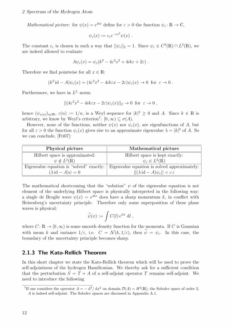
Mathematical picture: for ψ(x) = eikx define for ε > 0 the function ψε : R→ C,
ψε(x) := cεe−εx2
ψ(x) .
The constant cε is chosen in such a way that ||ψε||2 = 1. Since ψε ∈ C2(R) ∩ L2(R), weare indeed allowed to evaluate
Aψε(x) = ψε(k2 − 4ε2x2 + 4ikε+ 2ε) .
Therefore we find pointwise for all x ∈ R:
(k2 id− A)ψε(x) = (4ε2x2 − 4ikεx− 2ε)ψε(x)→ 0 for ε→ 0 .
Furthermore, we have in L2–norm:
||(4ε2x2 − 4ikεx− 2ε)ψε(x)||2 → 0 for ε→ 0 ,
hence (ψε(n))n∈N, ε(n) := 1/n, is a Weyl sequence for |k|2 ≥ 0 and A. Since k ∈ R isarbitrary, we know by Weyl’s criterion7: [0 ,∞) ⊆ σ(A).
However, none of the functions, neither ψ(x) nor ψε(x), are eigenfunctions of A, butfor all ε > 0 the function ψε(x) gives rise to an approximate eigenvalue λ = |k|2 of A. Sowe can conclude, [Fri07]:
Physical picture Mathematical picture
Hilbert space is approximated: Hilbert space is kept exactly:ψ /∈ L2(R) ψε ∈ L2(R)
Eigenvalue equation is “solved” exactly: Eigenvalue equation is solved approximately:(λ id− A)ψ = 0 ||(λ id− A)ψε|| < c ε
The mathematical shortcoming that the “solution” ψ of the eigenvalue equation is notelement of the underlying Hilbert space is physically interpreted in the following way:a single de Broglie wave ψ(x) = eikx does have a sharp momentum k, in conflict withHeisenberg’s uncertainty principle. Therefore only some superposition of these planewaves is physical:
ψ(x) :=
∫C(l) eilx dl ,
where C : R→ [0 ,∞) is some smooth density function for the momenta. If C is Gaussian
with mean k and variance 1/ε, i.e. C = N (k, 1/ε), then ψ = ψε. In this case, theboundary of the uncertainty principle becomes sharp.
2.1.3 The Kato-Rellich Theorem
In this short chapter we state the Kato-Rellich theorem which will be used to prove theself-adjointness of the hydrogen Hamiltonian. We thereby ask for a sufficient conditionthat the perturbation S = T + A of a self-adjoint operator T remains self-adjoint. Weneed to introduce the following
7If one considers the operator A = − d2/ dx2 on domain D(A) = H2(R), the Sobolev space of order 2,A is indeed self-adjoint. The Sobolev spaces are discussed in Appendix A.1.
12
2.1 Non-relativistic Schrodinger Model
Definition 2.27. Let A, T : X → Y be two linear operators in X with D(T ) ⊆ D(A).The operator A is called T -bounded if there are constants a, b ≥ 0 such that
||Ax|| ≤ a||x||+ b||Tx|| for all x ∈ D(T ) . (2.5)
In this case we define the T -bound of A by
b0 := infb ≥ 0 : there is a ≥ 0 such that (2.5) holds .
Remark 2.28. If A ∈ B(X, Y ), then A is T -bounded for all linear operators T : X → Yin X with b0 = 0 and a = ||A||. However, in general it is not possible to fulfill (2.5) whensetting b = b0.
Theorem 2.29. Kato-RellichLet T : X → X be a self-adjoint linear operator in X. If A : X → X is hermitianand T -bounded with T -bound b0 < 1, then the perturbed operator S := T + A is again aself-adjoint operator in X with domain D(S) = D(T ).
Proof. We refer to the literature, for instance [RS75].
2.1.4 Self-adjointness of the Hydrogen Hamiltonian
In this section our main goal is to show that the hydrogen Hamiltonian,
H = −1
2∆− 1
|x| , (2.6)
is a self-adjoint operator in L2(R3) with domain H2(R3). Here, Hk denotes the Sobolevspace of order k which is described in Appendix A.1. The structure of this operator ismotivated by classical physics and the correspondence principle.
Consider a classical particle with mass m > 0, velocity v ∈ R3 and momentum p =mv ∈ R3. The kinetic energy of this particle reads T = mv2/2 = p2/2m ∈ R. In anattractive Coulomb potential where this particle with elementary charge e < 0 interactswith some other particle with charge −e > 0, its potential energy reads V = −e2/4πε0|x|.In classical Hamilton theory, the total energy is just the sum H = T +V ∈ R. We are notgoing to use SI units and switch to units such that m = 1, ~ = 1 and e2 = 4πε0. So farthe particle is considered classically. Mapping the energy H to an operator by identifyingthe momentum p with an operator, p 7→ −i∇, we find H to be the operator stated in(2.6). This way of motivating the hydrogen Hamiltonian by mapping classical observablesto operators is called correspondence principle.
Remark 2.30. The hydrogen Hamiltonian (2.6) is a so-called Schrodinger operator,since it is a linear operator in the Hilbert space L2(Rn) and obeys the form ∆ +V , whereV is some real-valued function.
Theorem 2.31. Let A : L2(Rn) → L2(Rn) be the linear operator A = −∆. On thedomain H2(Rn), A = −∆ is self-adjoint and σ(−∆) = σess(−∆) = [0 ,∞).
Proof. For both, the proof of self-adjointness and the proof for the spectrum, we refer tothe literature, for instance to [HS96]. Crucial ingredients for the second part of the proofare Fourier analysis and Weyl’s criterion 2.24.
13
2 Spectrum of the Hydrogen Atom
For showing that not only the unperturbed Laplacian is self-adjoint on H2(Rn), but alsothe hydrogen Hamiltonian (2.6), we need the following
Theorem 2.32. Hardy’s inequalityLet n ∈ N with n ≥ 3, then one has for all f ∈ H1(Rn):∫
Rn
|f(x)|2|x|2 dx ≤ 4
(n− 2)2
∫Rn|∇f(x)|2 dx . (2.7)
Proof. We assume without loss of generality that f ∈ H1(Rn) is a real-valued function.Then, we have for all i = 1, . . . , n and all α ∈ R:
0 ≤∫Rn
[∂if(x)− α xi
|x|2f(x)
]2
dx =
∫Rn
[(∂if(x))2 − 2α
xi|x2|f(x)∂if(x) +
α2x2i
|x|4 f(x)2
]dx .
The second term reads∫Rn−α xi|x|2∂if(x)2 dx = α
∫Rn
(∂ixi|x|2
)f(x)2 dx = α
∫Rn
(1
|x|2 − 2x2i
|x|4)f(x)2 dx ,
where we used ∂if2 = 2f∂if and integrated by parts. Since f ∈ H1(Rn), there is no
surface term. Summing now over all components, i = 1, . . . , n, yields
0 ≤∫Rn
[|∇f(x)|2 + α
(n
|x|2 −2
|x|2)f(x)2 +
α2
|x|2f(x)2
]dx =
=
∫Rn
[|∇f(x)|2 +
(α(n− 2) + α2
) f(x)2
|x|2]
dx .
Both terms, |∇f(x)|2 and f(x)2/|x|2 are non-negative. Therefore, we find an optimalbound when minimizing over α:
α(n− 2) + α2 = min ⇔ α =2− nn
.
At this minimizer, the inequality reads:
0 ≤∫Rn
[|∇f(x)|2 − (n− 2)2
4
f(x)2
|x|2]
dx ,
which implies the claim.
Remark 2.33. The presented proof of Hardy’s inequality is adapted from [Fri07]. Forthe proof and, actually, also for the inequality (2.7), the hypothesis n ≥ 3 is necessary,since the left-hand side of Hardy’s inequality,
∫Rnf(x)2/|x|2 dx, might be divergent for
n = 1 or n = 2.
Remark 2.34. In [RS75] a special case of Hardy’s inequality is proven: there, the so-called“uncertainty principle” states that (2.7) holds for all f ∈ C∞0 (R3) ⊆ H1(R3). However,in the literature there are other versions of Hardy’s inequality, too. For instance, in[GGM03], there is an Lp-version for f ∈ W 1,p
0 , p ≥ 1.
Now we are able to prove our claim that the hydrogen Hamiltonian in at least threedimensions and on a suitable domain is a self-adjoint operator:
14
2.1 Non-relativistic Schrodinger Model
Theorem 2.35. Let H : L2(Rn)→ L2(Rn) be the hydrogen Hamiltonian H = −12∆− 1
|x| .
If n ≥ 3, then H is a self-adjoint operator on D(H) = H2(Rn).
Proof. Consider in L2(Rn) the linear operator T = −12∆ with domain D(T ) = H2(Rn).
Furthermore consider on L2(Rn) the linear operator A with Aψ(x) = − 1|x|ψ(x) . We show
that A is T -bounded with T -bound b0 < 1: for ψ ∈ L2(Rn) we have:
||Aψ||22 = || 1
|x|ψ||22 =
∫Rn
1
|x|2 |ψ(x)|2 dx ≤ 4
(n− 2)2
∫Rn|∇ψ(x)|2 dx =
=4
(n− 2)2
∫Rn∇ψ(x) · ∇ψ(x) dx =
4
(n− 2)2
∫Rn
(−∆ψ(x))ψ(x) dx ≤
≤ 4
(n− 2)2||∆ψ||2 ||ψ||2 ,
where we used first Hardy’s inequality8, subsequently the Cauchy-Schwarz inequality.Consider now some ε > 0, then one has for all a, b ≥ 0:
0 ≤(εa− b
ε
)2
= ε2a2 − 2ab+b2
ε2, hence ab ≤ 1
2
(ε2a2 +
b2
ε2
).
Therefore we find:
||Aψ||22 ≤2
(n− 2)2
(ε2||∆ψ||22 +
1
ε2||ψ||22
).
Using√a+ b ≤ √a+
√b for a, b ≥ 0, we finally arrive at:
||Aψ||2 ≤√
2
n− 2
(ε||∆ψ||2 +
1
ε||ψ||2
)=
2√
2
n− 2
(ε||Tψ||2 +
1
2ε||ψ||2
).
Choose 0 < ε < n−22√
2, then A is indeed T -bounded with T -bound b0 < 1. By Theorem 2.31,
T is self-adjoint, hence applying the Kato-Rellich theorem 2.29 finishes the proof.
2.1.5 Non-relativistic Spectrum of the Hydrogen Atom
For later convenience we introduce an additional parameter, Z ∈ N, describing the nu-clear charge of the hydrogen-type Hamiltonian9. Later on, when discussing the PTmodel, this parameter will be crucial for our approach to many-electron systems.
Theorem 2.36. For Z ∈ N, let H = −12∆ − Z
|x| be a linear operator in L2(R3) with
domain D(H) = H2(R3). Then
(a) H is a self-adjoint operator with σ(H) = −Z2/2n2 : n ∈ N ∪ [0 ,∞) .
(b) For all n ∈ N, En := −Z2/2n2 is an eigenvalue of H. Its corresponding eigenspaceis n2–dimensional, En ∈ σdisc(H).
8The hypothesis of Theorem 2.32 is fulfilled, since H2(Rn) ⊆ H1(Rn).9For X being some chemical element, we call an ion “X–like” if it has as many electrons as the neutral
one, N , but some arbitrary nuclear charge Z ≥ N , compare Definition 3.9. Note that for being astable ion, the condition Z ≥ N must be fulfilled, compare [Fri03].
15
2 Spectrum of the Hydrogen Atom
Proof. We show only some aspects of the theorem. For the complete proof we refer to theliterature, for instance [Fri07].
(a) First we show that [0 ,∞) ⊆ σ(H) by proving that
ψn(x) =1
(2εn)3/4exp
(−(x− an)2
4εn+ ik(x− an)
)(2.8)
denotes for some εn > 0 and an ∈ R3 a Weyl sequence for H and λ = 12|k|2. One
finds immediately that ||ψn||2 = 1 for all n ∈ N. Applying 12∆ to ψn, one gets:
1
2∆ψn(x) = ψn(x)
[x2
8ε2n
− ix · k2εn
− x · an4ε2
n
+a2n
8ε2n
+ian · k
2εn− 3
4εn− k2
2
].
The last term is canceled by λψn(x) and we arrive at∥∥∥∥(λ id +1
2∆ +
Z
|x|
)ψn(x)
∥∥∥∥2
2
≤∥∥∥∥ x2
8ε2n
ψn
∥∥∥∥2
2
+
∥∥∥∥ a2n
8ε2n
ψn
∥∥∥∥2
2
+
∥∥∥∥x · an4ε2n
ψn
∥∥∥∥2
2
+
∥∥∥∥ 3
4εnψn
∥∥∥∥2
2
+
+
∥∥∥∥x · k2εnψn
∥∥∥∥2
2
+
∥∥∥∥an · k2εnψn
∥∥∥∥2
2
+
∥∥∥∥ Z|x|ψn∥∥∥∥2
2
.
(2.9)We consider now a sequence 0 < εn → ∞ for n → ∞ and choose an := a0
√εn,
with 0 6= a0 ∈ R3. With this, we find that all terms on the right-hand side of (2.9)vanish in the limit n → ∞, since for all of them there is some q < 0 such that|| · || = εqn · const. As instructive example we derive the third term explicitly:∥∥∥∥x · an4ε2
n
ψn
∥∥∥∥2
2
=1
16ε4n
∫R3
√εn(x · a0)2
(2πεn)3/2exp
(−(x− a0
√εn)2
2εn
)dx =
=1
16(2π)3/2
1
ε2n
∫R3
(x · a0)2 exp
(−(x− a0)2
2
)dx =
1
ε2n
· const.
In the second line we have switched to x := x/√εn. The remaining three-dimensional
integral is a finite constant, hence
limn→∞
∥∥∥∥x · an4ε2n
ψn
∥∥∥∥2
2
= 0 .
Similar calculations lead to q = −2 for the expressions of the first line in (2.9) andto q = −1 in the second line. Altogether we arrive at
limn→∞
∥∥∥∥(1
2k2 id−H
)ψn
∥∥∥∥2
= 0 . (2.10)
Since k ∈ R3 is arbitrary, Weyl’s criterion 2.23 implies the claim [0 ,∞) ⊆ σ(H).
(b) In Appendix A.2 we show that En = −Z2/2n2 < 0 is an eigenvalue of H. Thecorresponding eigenspace is spanned by the orthonormal basis
Vn = ψnlm ∈ L(R3) : l = 0, 1, . . . , n−1 and m = −l,−l+1, . . . , l−1, l . (2.11)
16
2.1 Non-relativistic Schrodinger Model
The ψnlm are eigenfunctions of H, given in Theorem A.16:
ψnml(r, θ, ϕ) = Z3/2Rnl(Zr)Ylm(θ, ϕ) ,
where Ylm denote the spherical harmonics and Rnl are principally governed by theassociated Laguerre polynomials. However, we can calculate quickly the number ofelements in Vn:
#Vn =n−1∑l=0
(2l + 1) = n2 . (2.12)
Together we have En ∈ σ(H) and dim spanVn = n2 <∞, hence En ∈ σdisc(H).
In the PT model and for the discussion of its relativistic corrections, the hydrogen orbitals,ψnlm, are crucial. The following table states their explicit form for the lowest quantumnumbers n = 1 and n = 2:
n l m ψnlm(r, θ, ϕ) ψnlm(x) notation
1 0 0 Z3/2√πe−Zr Z3/2
√πe−Z|x| |1〉
2 0 0 Z3/2√
8π
(1− Zr
2
)e−Zr/2 Z3/2
√8π
(1− Z|x|
2
)e−Z|x|/2 |2〉
1 0 Z5/2√
32πr cos θ e−Zr/2 Z5/2
√32π
x3 e−Z|x|/2 |3〉
1 Z5/2√
32πr sin θ cosϕ e−Zr/2 Z5/2
√32π
x1 e−Z|x|/2 |4〉
−1 Z5/2√
32πr sin θ sinϕ e−Zr/2 Z5/2
√32π
x2 e−Z|x|/2 |5〉
Table 2.1: Hydrogen orbitals for the lowest quantum numbers n = 1 and n = 2. For the state (n, l,m) =(2, 1,±1) we have chosen the real part, |4〉, and imaginary part, |5〉, of exp (±imϕ) insteadof their complex linear combination. This is just a change of the basis functions and moreconvenient for later use.
17
2 Spectrum of the Hydrogen Atom
2.2 Relativistic Dirac Model
Es gibt keinen Gott und Dirac ist sein Prophet.10
Wolfgang Pauli
When quantum mechanics arose in the 20th of the last century, the special and generaltheory of relativity was already known and largely accepted. One of the big shortcom-ings of early quantum mechanics was the fact that its fundamental equation of motion,namely the Schrodinger equation, was violating relativistic symmetry aspects: the timeappears in a first-order derivative, whereas the spatial momentum appears in a second-order derivative. In principle, one can remove this flaw by implementing the relativisticenergy-momentum relation, E2 = p2 +m2, and, by the correspondence principle betweenobservables and operators, one can therewith motivate the relativistic Klein-Gordon equa-tion. In the first time it was not clear how to interpret its solutions. Today, withinquantum field theory, the Klein-Gordon equation itself and its physical conclusions areunderstood. However, we are not going to discuss these aspects and refer to the literature,for instance [PS95].
In order to describe relativistic particles with half-integer spin, so-called fermions, rela-tivistic quantum mechanics11 tells us to use the Dirac equation instead of the Klein-Gordonequation. The latter one describes relativistic particles with integer spin, so-called bosons.Our main goal of this section is to introduce the free Dirac operator, H0, and its cou-pling to the Coulomb potential. For later use in the PT model, we also prepare thenon-relativistic limit, H∞, and its first-order relativistic corrections. We refer mostly to[Tha92].
2.2.1 Self-adjointness of the Dirac Operator
Definition 2.37. Consider the Hilbert space X = L2(R3,C4) = L2(R3)⊗C4, i.e. the setof all L2–functions ψ : R3 → C4. The scalar product of ψ, φ ∈ X is defined by
〈ψ, φ〉X :=4∑i=1
〈ψi, φi〉 ,
where 〈·, ·〉 is the usual scalar product on L2(R3). We define the in L2(R3)⊗C4 the linearfree Dirac operator12
H0 := −ic0α · ∇+ βc20 , (2.13)
10There is no God and Dirac is his prophet.11Actually relativistic quantum mechanics is already a quantum field theory, since there is no relativistic
theory of one-particle quantum systems. Having the possibility of converting energy and mass, as thespecial theory of relativity states, the number of particles is no longer a well-defined quantity of thesystem. The idea of fields accommodates this physical principle in a very successful way, as QED,QCD and the whole Standard Model show. One of the paradoxes when holding on to the one-particlepicture is the Klein paradox which is discussed frequently in the physical literature.
12Again, we use atomic units, hence our Dirac operator is adapted to a fermion with mass m = 1. Lateron, for the discussion of the non-relativistic limit, we need the explicit dependence of H0 on thespeed of light c0. In atomic units one has c0 = 1/α0 ≈ 137, where α0 denotes the electromagneticfine-structure constant.
18
2.2 Relativistic Dirac Model
where c0 > 0 is some parameter and (β, α) is a four-component vector with complex 4×4matrices:
β :=
(12 00 −12
)and αi :=
(0 σiσi 0
)i = 1, 2, 3 ,
where the complex 2× 2 matrices σi, i = 1, 2, 3, are the so-called Pauli matrices, listedand briefly discussed in Appendix A.3.
Remark 2.38.
(i) It is beyond the scope of this thesis to justify the form of the matrices α and βfrom a group-theoretic point of view. However, our choice is called the Pauli-Dirac representation and is convenient for our purpose, since β, also called γ0,is diagonal. For a deeper examination of this, we refer to the multifarious physicalliterature, for instance [PS95].
(ii) From a mathematical point of view, the four-component complex wave functionsψ ∈ L2(R3) ⊗ C4 are vectors. However, in physics they are called Dirac spinors,due to their transformation law under some Lorentz transformation (ω, ϕ), whereω, ϕ ∈ R3 denote some boost and spatial rotation, respectively:
ψ′ =
exp(i2
∑3j=1 σj(ϕj − iωj)
)0
0 exp(i2
∑3j=1 σj(ϕj + iωj)
) ψ .
We emphasize that, although ψ being a four-component vector, ψ is not a (rela-tivistic) four-vector in the common physical nomenclature.
Our next step is the investigation of the domain of the free Dirac operator and its spec-trum. With the following, we will be able to define the Foldy-Wouthuysen transformation,UFW , which transforms the free Dirac operator into a diagonal matrix differential opera-tor.
For n ∈ N consider the well-known Fourier transformation F : L1(Rn)→ C(Rn), whichmaps integrable functions, ψ ∈ L1(Rn), to continuous functions, Fψ ∈ C(Rn), by
(Fψ)(p) :=1
(2π)n/2
∫Rnψ(x)e−ip·x dx . (2.14)
The Fourier transformation is a linear map on the Banach space of integrable functionsonto some complicated and cumbersome subspace of the set of continuous functions onRn. In fact, it may happen that the Fourier transform of ψ ∈ L1(Rn) is not again inte-grable: Fψ /∈ L1(Rn). In order to define a more handy version of the Fourier transforma-tion, firstly we restrict F to L1(Rn) ∩ L2(Rn), which is a dense subspace of the Hilbertspace L2(Rn). Second, by Plancherel’s theorem13, this restricted Fourier transformation,F|L1∩L2 , can be uniquely extended to some unitary operator14 P : L2(Rn) → L2(Rn),called the Plancherel transformation. Note that P is a continuous linear operator onL2(Rn) onto L2(Rn) and ||Pψ||2 = ||ψ||2 for all ψ ∈ L2(Rn).
13Plancherel’s theorem is discussed frequently in the literature, for instance in [Eva98] or [RS75].14A linear operator A : X → X in a Hilbert space X is called unitary, if it is isometric on X, i.e.||Ax|| = ||x|| for all x ∈ X.
19
2 Spectrum of the Hydrogen Atom
Remark 2.39. We want to emphasize that the Plancherel transformation, P , does notextend the Fourier transformation, F , although it is sometimes stated in the literature.Note that in the first place F is defined on L1(Rn), but the restriction of the Planchereltransformation to this space, P|L1 : L1(Rn) ∩ L2(Rn) → L2(Rn), is not defined for allintegrable functions. However, it is possible that the Lp spaces are nested: if one considersthe counting measure on N, then Lp = lp and the inclusion l1 ⊆ l2 holds.
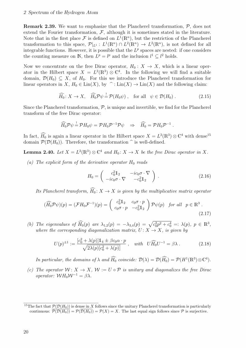
Now we concentrate on the free Dirac operator, H0 : X → X, which is a linear oper-ator in the Hilbert space X = L2(R3) ⊗ C4. In the following we will find a suitabledomain, D(H0) ⊆ X, of H0. For this we introduce the Plancherel transformation forlinear operators in X, H0 ∈ Lin(X), by : Lin(X)→ Lin(X) and the following claim:
H0 : X → X, H0Pψ !=P(H0ψ) , for all ψ ∈ D(H0) . (2.15)
Since the Plancherel transformation, P , is unique and invertible, we find for the Planchereltransform of the free Dirac operator:
H0Pψ !=PH0ψ = PH0P−1Pψ ⇒ H0 = PH0P−1 .
In fact, H0 is again a linear operator in the Hilbert space X = L2(R3)⊗C4 with dense15
domain P(D(H0)). Therefore, the transformation is well-defined.
Lemma 2.40. Let X = L2(R3)⊗ C4 and H0 : X → X be the free Dirac operator in X.
(a) The explicit form of the derivative operator H0 reads
H0 =
(c2
012 −ic0σ · ∇−ic0σ · ∇ −c2
012
). (2.16)
Its Plancherel transform, H0 : X → X is given by the multiplicative matrix operator
(H0Pψ)(p) = (FH0F−1)(p) =
(c2
012 c0σ · pc0σ · p −c2
012
)Pψ(p) for all p ∈ R3 .
(2.17)
(b) The eigenvalues of H0(p) are λ1,2(p) = −λ3,4(p) =√c2
0p2 + c4
0 =: λ(p), p ∈ R3,where the corresponding diagonalization matrix, U : X → X, is given by
U(p)±1 :=[c2
0 + λ(p)]14 ± βc0α · p√2λ(p)[c2
0 + λ(p)], with UH0U
−1 = βλ . (2.18)
In particular, the domains of λ and H0 coincide: D(λ) = D(H0) = P(H1(R3)⊗C4).
(c) The operator W : X → X, W := U P is unitary and diagonalizes the free Diracoperator: WH0W−1 = βλ.
15The fact that P(D(H0)) is dense in X follows since the unitary Plancherel transformation is particularlycontinuous: P(D(H0)) = P(D(H0)) = P(X) = X. The last equal sign follows since P is surjective.
20
2.2 Relativistic Dirac Model
Proof.
(a) The explicit form of the free Dirac operator H0 in (2.17) follows directly from thedefinition of the matrices β and α. For its Plancherel transform, (2.14) tells us to
map16 ∇ 7→ ip, which implies directly H0.
(b) A straightforward calculation yields for p ∈ R3 the eigenvalues±λ(p) = ±√c2
0p2 + c4
0
of H0, and also the unitary matrix U(p) which diagonalizes H0:
(UH0U−1)(p) = βλ(p) .
For the inverse matrix U(p)−1 one uses the anti-commutator relation αi, β = 0,i = 1, 2, 3. Furthermore, the identities β2 = 14 and (α · p)(α · p) = p2 hold.
Note that the eigenvalue operator λ : X → X is just a multiplication operator,P(D(H0)) 3 Pψ 7→ λ(p)14Pψ(p), for all p ∈ R3. Since U : X → X is unitary and
β a constant matrix, the domains of H0 and λ coincide: D(H0) = D(λ). The formof the eigenvalues ±λ(p) implies17
D(λ) =Pψ ∈ X :
√1 + p2 (Pψ)(p) ∈ X
. (2.19)
Therefore, using for k = 1 and n = 3 the equivalent definitions of the Sobolev spacesHk(Rn) in Theorem A.8 (i) ⇔ (iii), we find
Pψ ∈ D(λ) ⇔√
1 + p2 (Pψ)(p) ∈ L2(R3)⊗ C4 ⇔ ψ ∈ H1(R3)⊗ C4 ,(2.20)
hence D(H0) = D(λ) = P(H1(R3)⊗ C4).
(c) As composition of two unitary operators, U and P on X, the operator W = U Pis unitary, too. Using the results of part (a) and (b), we find immediately:
WH0W−1 = UPH0P−1U−1 = UH0U−1 = βλ . (2.21)
Theorem 2.41. The free Dirac operator H0 in X = L2(R3)⊗C4 is a self-adjoint operatoron D(H0) = H1(R3)⊗ C4. Its spectrum is given by σ(H0) = (−∞,−c2
0] ∪ [c20,∞).
Proof. From (2.15) we know D(H0) = P(D(H0)). Since the Plancherel transformation is
unitary we have D(H0) = P−1(D(H0)). Combining this we Lemma 2.40(b), particularly
D(λ) = D(H0) = P(H1(R3) ⊗ C4), we find: D(H0) = H1(R3) ⊗ C4. Furthermore, fromLemma 2.40(c) we know that the operator H0 is unitarily equivalent to the multiplicativediagonal operator βλ, hence
σ(H0) = σ(βλ) = ranλ1,2(·) ∪ ranλ3,4(·) = (−∞,−c20] ∪ [c2
0,∞) .
For the remaining proof of the self-adjointness we refer to the short proof in [Tha92].
16Note that we have already met this mapping for motivating the hydrogen Hamiltonian (2.6): p 7→ −i∇.17At this point it is important that the particle is massive, i.e. m > 0, since we are scaling, i.e. dividing
by the constant m2c40. However, we work in atomic units, hence we are not affected by this restriction.In the massless case the here made implication would be not correct.
21
2 Spectrum of the Hydrogen Atom
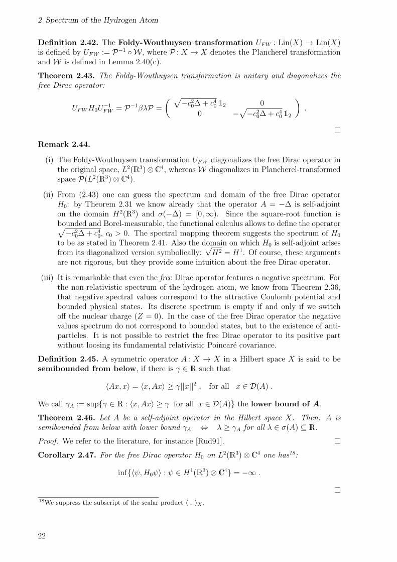
Definition 2.42. The Foldy-Wouthuysen transformation UFW : Lin(X) → Lin(X)is defined by UFW := P−1 W , where P : X → X denotes the Plancherel transformationand W is defined in Lemma 2.40(c).
Theorem 2.43. The Foldy-Wouthuysen transformation is unitary and diagonalizes thefree Dirac operator:
UFWH0U−1FW = P−1βλP =
( √−c2
0∆ + c40 12 0
0 −√−c2
0∆ + c40 12
).
Remark 2.44.
(i) The Foldy-Wouthuysen transformation UFW diagonalizes the free Dirac operator inthe original space, L2(R3)⊗C4, whereas W diagonalizes in Plancherel-transformedspace P(L2(R3)⊗ C4).
(ii) From (2.43) one can guess the spectrum and domain of the free Dirac operatorH0: by Theorem 2.31 we know already that the operator A = −∆ is self-adjointon the domain H2(R3) and σ(−∆) = [0 ,∞). Since the square-root function isbounded and Borel-measurable, the functional calculus allows to define the operator√−c2
0∆ + c40, c0 > 0. The spectral mapping theorem suggests the spectrum of H0
to be as stated in Theorem 2.41. Also the domain on which H0 is self-adjoint arisesfrom its diagonalized version symbolically:
√H2 = H1. Of course, these arguments
are not rigorous, but they provide some intuition about the free Dirac operator.
(iii) It is remarkable that even the free Dirac operator features a negative spectrum. Forthe non-relativistic spectrum of the hydrogen atom, we know from Theorem 2.36,that negative spectral values correspond to the attractive Coulomb potential andbounded physical states. Its discrete spectrum is empty if and only if we switchoff the nuclear charge (Z = 0). In the case of the free Dirac operator the negativevalues spectrum do not correspond to bounded states, but to the existence of anti-particles. It is not possible to restrict the free Dirac operator to its positive partwithout loosing its fundamental relativistic Poincare covariance.
Definition 2.45. A symmetric operator A : X → X in a Hilbert space X is said to besemibounded from below, if there is γ ∈ R such that
〈Ax, x〉 = 〈x,Ax〉 ≥ γ||x||2 , for all x ∈ D(A) .
We call γA := supγ ∈ R : 〈x,Ax〉 ≥ γ for all x ∈ D(A) the lower bound of A.
Theorem 2.46. Let A be a self-adjoint operator in the Hilbert space X. Then: A issemibounded from below with lower bound γA ⇔ λ ≥ γA for all λ ∈ σ(A) ⊆ R.
Proof. We refer to the literature, for instance [Rud91].
Corollary 2.47. For the free Dirac operator H0 on L2(R3)⊗ C4 one has18:
inf〈ψ,H0ψ〉 : ψ ∈ H1(R3)⊗ C4 = −∞ .
18We suppress the subscript of the scalar product 〈·, ·〉X .
22
2.2 Relativistic Dirac Model
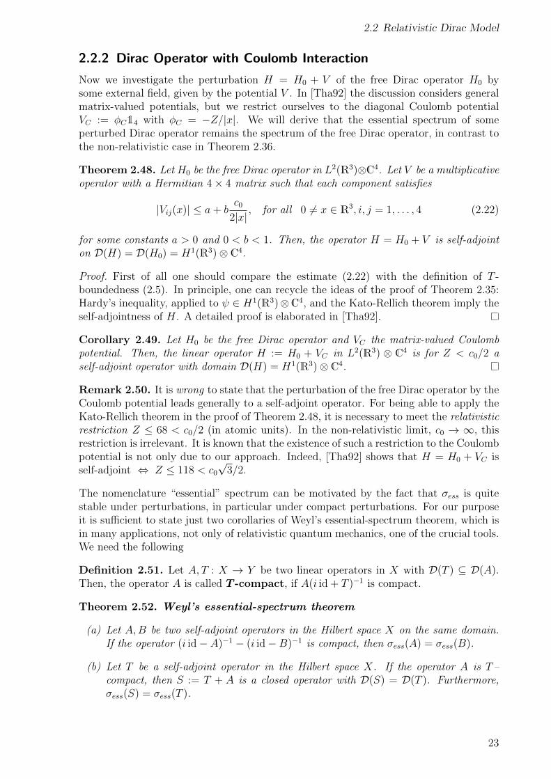
2.2.2 Dirac Operator with Coulomb Interaction
Now we investigate the perturbation H = H0 + V of the free Dirac operator H0 bysome external field, given by the potential V . In [Tha92] the discussion considers generalmatrix-valued potentials, but we restrict ourselves to the diagonal Coulomb potentialVC := φC14 with φC = −Z/|x|. We will derive that the essential spectrum of someperturbed Dirac operator remains the spectrum of the free Dirac operator, in contrast tothe non-relativistic case in Theorem 2.36.
Theorem 2.48. Let H0 be the free Dirac operator in L2(R3)⊗C4. Let V be a multiplicativeoperator with a Hermitian 4× 4 matrix such that each component satisfies
|Vij(x)| ≤ a+ bc0
2|x| , for all 0 6= x ∈ R3, i, j = 1, . . . , 4 (2.22)
for some constants a > 0 and 0 < b < 1. Then, the operator H = H0 + V is self-adjointon D(H) = D(H0) = H1(R3)⊗ C4.
Proof. First of all one should compare the estimate (2.22) with the definition of T -boundedness (2.5). In principle, one can recycle the ideas of the proof of Theorem 2.35:Hardy’s inequality, applied to ψ ∈ H1(R3)⊗C4, and the Kato-Rellich theorem imply theself-adjointness of H. A detailed proof is elaborated in [Tha92].
Corollary 2.49. Let H0 be the free Dirac operator and VC the matrix-valued Coulombpotential. Then, the linear operator H := H0 + VC in L2(R3) ⊗ C4 is for Z < c0/2 aself-adjoint operator with domain D(H) = H1(R3)⊗ C4.
Remark 2.50. It is wrong to state that the perturbation of the free Dirac operator by theCoulomb potential leads generally to a self-adjoint operator. For being able to apply theKato-Rellich theorem in the proof of Theorem 2.48, it is necessary to meet the relativisticrestriction Z ≤ 68 < c0/2 (in atomic units). In the non-relativistic limit, c0 → ∞, thisrestriction is irrelevant. It is known that the existence of such a restriction to the Coulombpotential is not only due to our approach. Indeed, [Tha92] shows that H = H0 + VC isself-adjoint ⇔ Z ≤ 118 < c0
√3/2.
The nomenclature “essential” spectrum can be motivated by the fact that σess is quitestable under perturbations, in particular under compact perturbations. For our purposeit is sufficient to state just two corollaries of Weyl’s essential-spectrum theorem, which isin many applications, not only of relativistic quantum mechanics, one of the crucial tools.We need the following
Definition 2.51. Let A, T : X → Y be two linear operators in X with D(T ) ⊆ D(A).Then, the operator A is called T -compact, if A(i id + T )−1 is compact.
Theorem 2.52. Weyl’s essential-spectrum theorem
(a) Let A,B be two self-adjoint operators in the Hilbert space X on the same domain.If the operator (i id− A)−1 − (i id−B)−1 is compact, then σess(A) = σess(B).
(b) Let T be a self-adjoint operator in the Hilbert space X. If the operator A is T–compact, then S := T + A is a closed operator with D(S) = D(T ). Furthermore,σess(S) = σess(T ).
23
2 Spectrum of the Hydrogen Atom
Proof. As already mentioned, both statements are actually corollaries of Weyl’s essential-spectrum theorem, which is proved, for instance, in [RS78].
Let X be a Hilbert space and M ⊆ X some open or closed subset. In the followingχM : X → 0, 1 will denote the characteristic function of M , i.e. χM(x) = 1 if x ∈ Mand χM(x) = 0 if x 6= M . Instead of χy∈X:||y||<R(x), R > 0, we will write moreconveniently χ(||x|| < R).
Lemma 2.53. Let A,B be two self-adjoint operators in the Hilbert space X on the samedomain. If one has for all λ ∈ C\R that
limR→∞
∥∥[(λ id− A)−1 − (λ id−B)−1]χ(||x|| ≥ R)
∥∥ = 0 , (2.23)
then the following two statements are equivalent:
(i) T := (λ id− A)−1 − (λ id−B)−1 is compact.
(ii) TR := [(λ id− A)−1 − (λ id−B)−1]χ(||x|| < R) is compact for all R > 0.
Proof. The implication (i) ⇒ (ii) follows directly by the fact that χ is just some multi-plicative bounded function, hence its product with a compact operator is again a compactoperator. Note that for this implication, (2.23) is not needed.
For the other direction, (ii)⇒ (i), consider
||TR − T || = ||[(λ id− A)−1 − (λ id−B)−1
]χ(||x|| ≥ R)|| → 0 for R→∞ .
This means TR converges to T in the norm topology. By hypothesis TR is a compactoperator for all R > 0. Using the fact that K(X, Y ), the space of compact operators inX to Y , is a closed subspace of B(X, Y ), the limit T is also compact.
Definition 2.54. A self-adjoint operator A : X → X in the Hilbert space X is calledlocally compact, if the operator (λ id−A)−kχ(||x|| < R) is compact for all R > 0, someλ ∈ C\R and some k > 0.
Lemma 2.55.
(a) If A is a locally compact, then (λ id − A)−kχ(||x|| < R) is compact for all R > 0,for all λ ∈ C\R and for all k > 0.
(b) Both, the free and the Coulomb-perturbed Dirac operator, H0 and H = H0 +VC, arelocally compact.
Proof. We refer to the literature: (a) is proven in [Per83], a proof of (b) can be found, forinstance, in [Tha92].
Finally, we are able to prove the main claim of this section: the essential spectrum of (allrelevant) Coulomb-perturbed Dirac operators is just the same as the (essential) spectrumof the free Dirac operator:
Theorem 2.56. Let H0 be the free Dirac operator and H = H0 + VC its perturbation byVC = φC14 with φC = −Z/|x| and Z < c0/2. One has σess(H) = σess(H0) = σ(H0).
24
2.2 Relativistic Dirac Model
Proof. The idea of the proof is to use Weyl’s essential-spectrum theorem 2.52(a). It issufficient to prove the compactness of (i id−H)−1 − (i id−H0)−1.
As the proof of Theorem 2.48 shows, VC is H0-bounded19, hence we are allowed to usethe second resolvent equation. With this, we get for all λ ∈ C\R:
limR→∞
∥∥[(λ id−H)−1 − (λ id−H0)−1]χ(||x|| ≥ R)
∥∥ =
= limR→∞
∥∥(λ id−H)−1VC(λ id−H0)−1χ(||x|| ≥ R)∥∥ ≤
≤ 1
|Imλ|2 limR→∞
‖φCχ(||x|| ≥ R)‖ ≤ 1
|Imλ|2 limR→∞
sup|x|≥R
Z
|x| = 0 ,
(2.24)
hence the hypothesis (2.23) holds. For the estimate we have used the identity
||(λ id− A)−1|| = 1
dist(λ, σ(A)),
which is true for self-adjoint operators A and λ ∈ ρ(A) = C\σ(A) ⊇ C\R, compare[Rud91].
Applying Lemma 2.55 (k = 1) yields that statement (ii) in Lemma 2.53 holds forall λ ∈ C\R. Therefore, in the special case λ = i, Lemma 2.53 (ii)⇒(i) implies thecompactness of (i id−H)−1 − (i id−H0)−1 and completes the proof.
2.2.3 Non-relativistic Limit and its Relativistic Corrections
We now derive the non-relativistic limit, H∞, of the Dirac operator H = H0 + V . Forthe following it is sufficient the potential V to be H0–bounded and symmetric, whichis fulfilled for the diagonal Coulomb potential V = VC . In the following, within thePT model, we will use this non-relativistic limit for investigating many electron-systems.Furthermore, we state the first-order corrections of the non-relativistic eigenvalues whichwe will need for our investigations of atomic spectra.
Consider the c0-dependent Dirac operator20 H(c0) = c0Q+c20β+VC in the Hilbert space
X = L2(R3) ⊗ C4 with domain D(H) = H1(R3) ⊗ C4, where Q = −iα · ∇. In order toget the physically-correct non-relativistic limit of the Dirac operator we need to subtractthe rest energy c2
0 from H(c0), since the rest energy does not have any correspondent inclassical non-relativistic physics. This statement becomes evident when considering therelativistic energy-momentum relation, E(p) =
√c2
0 + p2c40: when subtracting the rest
energy, c20, we get
E(p)− c20 =
p2
2− p4
8c20
+O(c−40 )→ T (p) for c0 →∞ , (2.25)
which is the classical kinetic energy T (p) of a particle with mass m = 1. The non-subtracted E(p) diverges for c0 →∞. However, even the operator H(c0)− c2
014 divergesfor c0 → ∞, hence H∞ = limc0→∞ (H(c0)− c2
014) is an ill-defined quantity and one hasto find another way to define H∞.
19This fact is crucial for being able to apply the Kato-Rellich theorem which proves the self-adjointnessof the perturbed operator H.
20In [Tha92] the setup of Dirac operators is more general: β can be substituted by some unitary involutionτ , and Q is allowed to be some (self-adjoint) supercharge with respect to τ .
25
2 Spectrum of the Hydrogen Atom
We use resolvents as an intermediate step and follow the ideas of [Ves69], elaboratedin [Tha92]. The key ingredient is the fact that the resolvent of H0(c0)− c2
0 is analytic in1/c0 around c0 =∞. We have the following
Theorem 2.57. Let H(c0) = c0Q + c20β + VC be the Dirac operator in X as described
above. Let A : X → X be the subtracted operator A := H(c0)− c2014. Then, the resolvent
RA(λ) is analytic in 1/c0 around c0 =∞ for all λ ∈ C\R with the expansion
RA(λ) =∞∑n=0
1
cn0Rn(λ) , (2.26)
where the right-hand side converges in the operator norm. The first two terms read
R0(λ) = R∞(λ)P+ = (λ id−H∞)−1P+ ,
R1(λ) = P+R∞(λ)1
2Q+
1
2QR∞(λ)P+ ,
(2.27)
where we defined H∞ := 12Q2 + VCP+ and its resolvent R∞(λ). Moreover, P+ denotes the
(positive) projection operator, defined by
P± :=1
2(14 ± β) =
1
2
(12 ± 12 0
0 12 ∓ 12
), (2.28)
with the properties21 P+P− = 0 = P−P+ and P 2± = P±.
Proof. We refer to [Tha92].
Corollary 2.58. We call H∞P+ the non-relativistic limit of the Dirac operator.Its explicit form reads
H∞P+ =
(−1
2∆− Z
|x|
)12 . (2.29)
Remark 2.59. Comparing H∞P+ with the definition of the hydrogen Hamiltonian in(2.6), we see that this is sort of doubling the former one. The physical reason for thisis given by the spin of the electron: as a particle with spin 1/2 there are two directionsof the spin (“up” and “down”), but the energy, described by the Hamiltonian, does notchange when changing the spin direction; this is true only in this non-relativistic limit.Introducing relativistic corrections, the energy of the system is actually dependent on thedirection of the electron spin.
Knowing the non-relativistic limit of the Dirac operator with Coulomb interaction, we arenow interested in relativistic corrections to its eigenvalues. As we know from Theorem2.36, the hydrogen Hamiltonian features, besides the non-negative essential spectrum,countably many isolated eigenvalues, En = −Z2/2n2, n ∈ N. The dimensions of alleigenspaces are finite: dim span Vn = n2. Taking the spin as additional degree of freedominto account, the eigenvalues of the non-relativistic limit H∞P+, are still En, but this timetheir multiplicity is given by 2n2.
21Note that both properties hold when replacing β by some unitary involution τ .
26
2.2 Relativistic Dirac Model
Theorem 2.60. Let H(c0) be as above. For all eigenvalues En of H∞P+ one has: theoperator H(c0) − c2
0 has k ≤ 2n2 distinct eigenvalues Ejn(c0), j = 1, . . . , k, whose multi-
plicities sum up to 2n2. Each Ej is analytic in 1/c0 around c0 =∞ with the expansion
Ejn(c0) = En +
1
c20
V jn +O(c−4
0 ) . (2.30)
The V jn , j = 1, . . . , k are eigenvalues of the self-adjoint matrix
Vab :=1
4〈ψa0 , Q(VC − En)Qψb0〉 , (2.31)
where ψa0 , a = 1, . . . , 2n2, forms an orthonormal system of eigenvectors of H∞P+ core-sponding to En.
In particular, for a non-degenerate eigenvalue22 of H∞P+ with eigenfunction |ψ0〉, thereis only one eigenvalue of the matrix V11:23
V11 = V 11 =
⟨ψ0
∣∣∣∣−p4
8+Z
2
L · S|x|3 +
πZ
2δ(3)(x)
∣∣∣∣ψ0
⟩, (2.32)
where we have defined the spin operator, S := 12σ and the angular-momentum oper-
ator L := −ix∧p, compare Definition 3.2. Moreover, δ(3) denotes the delta distributionin three dimensions, compare also the next Remark.
Proof. Again, we refer to [Tha92].
Remark 2.61.
(i) For a non-degenerate eigenvalue the matrix Vab in (2.32) is just one real number. Itsexplicit form is a straight-forward calculation, compare [Tha92]. The delta distribu-tion arises from the highly singular term ∆1/|x|. By the notation δ(3)(x) we targetthe following important property: 〈ψ0|δ(3)(x)|ψ0〉 = ψ0(0), which will be importantfor the explicit evaluation in Lemma 3.21.
(ii) For the degenerate eigenvalue En, n > 1, the matrix Vab, a, b = 1, . . . , n, mustbe diagonalized. In particular the LS-correction will force us to change the basislabeled with the quantum numbers (l, s), angular momentum and spin, and weneed to introduce the total angular momentum J := L + S. When discussingrelativistic corrections to the PT model, we will come back to this in detail.
(iii) It is important that the operators in (2.32) are evaluated by some well-behavingfunction |1〉 = Z3/2/
√π e−Z|x|. The operators (distributions) themselves are highly
singular and can not be treated isolated. The correction terms in (2.32) (in orderof their appearance) are called P-contribution, LS-coupling and Darwin term.The first one can be motivated by expanding the relativistic energy-momentumexpansion as done in (2.25). There, the P-contribution is just the c−4
0 -term in theexpansion. The LS-coupling is some magnetic effect, induced from the orbiting elec-tron. To get the right prefactor one has to take the Thomas precision into account.
22We call an eigenvalue λ non-degenerate, if its eigenspace is one-dimensional, otherwise we call λ adegenerate eigenvalue.
23We use the “bra-ket” notation which is frequently used in physics: 〈f |A|g〉 := 〈f,Ag〉 =∫Rn f
†(x)Ag(x) dx, where A denotes some linear operator and f, g ∈ D(A).
27
2 Spectrum of the Hydrogen Atom
The Darwin term can be considered as retardation effect of the electromagneticfield caused by the finite speed of light c0 <∞. For further reading we refer to theliterature [Sch07] and [PS95].
Definition 2.62. Motivated from (2.32) and using the notations in Table 2.1 we definefor i = 1, . . . , 5 the following notations:
IPi :=
⟨i
∣∣∣∣−p4
8
∣∣∣∣ i⟩ and IDi :=
⟨i
∣∣∣∣πZ2 δ(3)(x)
∣∣∣∣ i⟩ .
We conclude this section with the following
Remark 2.63. In the physical literature, for instance [Sch05], the corrections in (2.32) arederived using iteratively the Foldy-Wouthuysen transformation as introduced in (2.42).From a mathematical point of view, this approach is only formal and cannot be justifiedusing operator theory. The main problem thereby is the fact that doing perturbationtheory one needs, in some sense, a small quantity. Corrections like the P-contribution,−p4/8, destroy the applicability of perturbation theory on the operator level. Indeed, thereare examples where the Foldy-Wouthuysen transformation diverges when taking higher-order “corrections” into account, compare [Tha92]. The approach we have followed usesresolvents of operators as an intermediate step. This idea guarantees analyticity in 1/c0
around c0 =∞ and the convergence of the expansion (2.26) in the operator norm.
28
3 Spectrum of Many-electron Atoms
3.1 Non-relativistic Perturbation-theory Model
Physik ist die Kunst, die passende Naherung zu finden.Exakt rechnen kann jeder.1
Harald Friedrich
In this section we investigate atoms with more than one electron as in the hydrogen case.In these systems there are additional interactions we have to take into account. Even atthe non-relativistic level there is the Coulomb repulsion between the iso-charged electronswhich destroys the analytically solvability of the system.
In this first step we present the perturbation-theory (PT) model, developed in [FG09b]and [FG10], in which the interaction between the electrons can be treated perturbativelyif Z, the nuclear charge, is large. In this so-called asymptotic limit, the eigenfunctionsand their energy levels can be derived analytically. Taking these solutions as startingpoint, we are going to derive in a second step the relativistic corrections of these energylevels.
3.1.1 Definition of the PT Model
Considering the non-relativistic spectrum of a N -electron system, N ∈ N, we have to takeseveral aspects, some from physics, some from mathematics, into account. In the previouschapter of this thesis we have introduced and prepared all the ingredients we bring nowtogether. In the following we concentrate on the discrete spectrum, σdisc(H(N)), wherethe Hamiltonian H(N) is defined as
H(N) :=N∑i=1
(−1
2∆i −
Z
|xi|
)12 + Vee12 . (3.1)
H is just the sum of N copies of the non-relativistic limit of the Dirac equation withCoulomb interaction as derived in (2.29). The interaction between electrons is modeledby Vee and in the non-relativistic limit it restricts to a purely electromagnetic term
Vee :=∑
1≤i<j≤N
1
|xi − xj|=
1
2
∑i 6=j
1
|xi − xj|. (3.2)
The spin does not occur in the Hamiltonian H(N), hence the energies of the system,described by the eigenvalues, are independent of the spin. However, the underlying Hilbertspace knows about the spin:
X = L2a
((R3 × Z2)N
)⊗ C2 , (3.3)
1Physics is the art of finding a convenient approximation. Anybody is able to calculate accurately.
29
3 Spectrum of Many-electron Atoms
where L2a denotes the anti-symmetric2 subspace of L2, i.e. for all i, j = 1, . . . , N , i 6= j:
ψ(. . . , xi, si, . . . , xj, sj, . . .) = −ψ(. . . , xj, sj, . . . , xi, si, . . .) . (3.4)
Lemma 3.1. Denote H(N) the Hamiltonian of an N-electron system as defined above.H(N) is a linear operator in the Hilbert space X = L2
a
((R3 × Z2)N
)⊗ C2 with scalar
product
〈ψ, φ〉X :=2∑i=1
N∑j=1
∫R3
∑sj=± 1
2
ψ∗i (xj, sj)φi(xj, sj) dxj . (3.5)
Furthermore, H(N) is self-adjoint on the domain D(H) = (L2a ∩H2)((R3 × Z2)N)⊗ C2.
Proof. Mainly, this follows from Theorem 2.35: we find directly the self-adjointness ofH(N)−Vee12. The restriction to the subspace of anti-symmetric wave functions does notaffect this statement. For the self-adjointness of H(N) itself it is sufficient to show thatVee12 is (H(N)− Vee12)-bounded. This can be done similarly as in the proof of Theorem2.35.
For clarity, we compare the non-relativistic hydrogen Hamiltonian, H in (2.6), with theone-particle Hamiltonian, H(N = 1) = H∞L+ = H12, in detail: since 12 is just a unitymatrix, both operators feature the same eigenvalues, En = −Z2/2n2, but their eigenspacesdiffer. For H we know the corresponding bases: Vn, as given (2.11). Due to the spin,which occurs as additional degree of freedom, we define the Cartesian product
V σn := Vn × Z2 . (3.6)
This implies: dim span V σn = 2n2. For ψσnlm ∈ V σ
n we have
ψσnlm(x, s) = ψnlm(x)
[δ 1
2,s
(10
)+ δ− 1
2,s
(01
)]. (3.7)
Definition 3.2. We introduce the following operators (σ = (σ1, σ2, σ3) denotes the threePauli matrices, listed in Appendix A.3):
S :=N∑k=1
S(k) :=N∑k=1
1
2σ(k) spin angular momentum ,
L :=N∑k=1
L(k) :=N∑k=1
−ixk ∧∇k angular momentum ,
J := L+ S =N∑k=1
(L(k) + S(k)) total angular momentum .
The index k denotes that every term in the sum acts only on the k-th electron. Alloperators3 are defined on a suitable dense domain in the Hilbert space X, for instance
D(L) = ψ ∈ X : ||(x ∧∇)ψ||2X <∞ .2This restriction is caused by the Spin-Statistic Theorem [Pau40]. It states that elements ψ of a Hilbert
space which describe bosons are necessarily symmetric, whereas elements describing fermions arenecessarily anti-symmetric.
3To be more precise, one should write J := L12 + S.
30
3.1 Non-relativistic Perturbation-theory Model
Definition 3.3. Denote H some Hamiltonian defined in a Hilbert space X. A linearoperator A in X is called conserved quantity, if [H,A] := HA−AH = 0, on the densedomain D(H) ∩ D(A). Its eigenvalues are called good quantum numbers.
Remark 3.4. In physics, the eigenvalues of conserved quantities are called good quantumnumbers due to the following fact: a linear operator A is a conserved quantity if and onlyif the statement that ψ ∈ D(H)∩D(A) is an eigenfunction of H with eigenvalue E impliesthat Aψ is also an eigenfunction of H with the same eigenvalue. In this case, H and Ahave the same system of eigenfunctions.
The following lemma states one big difference between the non-relativistic Schrodingertheory and the relativistic Dirac theory: in a relativistic setup, the operators for angularmomentum and spin are no longer conserved quantities.
Lemma 3.5. Let be α as in Definition 2.37.
(a) For H(1) the operators L = L(1) and S = S(1) are conserved quantities.
(b) For H(N) the operators L and S are conserved quantities.
(c) For the Dirac operator with Coulomb interaction, H = H0 + φC14, one finds4
[H,S(k)] = α ∧∇ = −[H,L(k)] 6= 0 .
Instead, the total angular momentum is a conserved quantity: [H, J(k)] = 0.
Definition 3.6. We denote by H0(N) := H(N)− Vee12 the Hamiltonian which does notinclude the electron-electron interaction.5 Its ground state6 is denoted by V0(N). LetP be the orthogonal projection onto V0(N), then the PT Hamiltonian is defined byPH(N)P . The eigenvalue equation
PH(N)Pψ = Eψ, ψ ∈ V0(N) , (3.8)
is called the perturbation-theory (PT) model.
Remark 3.7. The nomenclature “perturbation theory” is justified by the following con-sideration: Let ψ be the solution of H(N)ψ = Eψ, then the scaled function
ψ(xi, si) := Z−3N/2 ψ(xi/Z, si), i = 1, . . . , N, (3.9)
solves the eigenvalue equation(H0(N) +
1
ZVee
)ψ =
E
Z2ψ . (3.10)
Therefore, the PT model represents just the leading-order term one would expect fromusual perturbation theory: for large Z the interaction term Vee can be neglected and theleading terms is governed by H0(N) and its eigenvalues.
4One has to interpret the operators suitably: S(k) 7→ S(k)⊗ 12, and L(k) 7→ (L(k)12)⊗ 12.5Note that despite using the subscript 0, H0(N) does not describe a free system, since H0(N) still
contains the Coulomb interaction between electrons and the nucleus.6It is known, [Fri03] that for neutral atoms and positive ions, N ≤ Z, there exist countably many
eigenvalues Ei ∈ σdisc(H(N)) with E1 < E2 < . . . The eigenspace corresponding to the energy valueE1 is called ground state.
31
3 Spectrum of Many-electron Atoms
3.1.2 Principal Results
In the following theorem we collect some of the constitutive properties of the PT model,justifying the ansatz and its nomenclature rigorously:
Theorem 3.8. Let N = 1, . . . , 10 be the fixed number of electrons, characterizing thechemical element we are dealing with. Let n(N) denote the number of energy levels of thePT model, then:
(a) for all sufficiently large Z, the lowest n(N) energy levels E1 < . . . < En(N), withEi = Ei(N,Z), of the full Hamiltonian H(N) have exactly the same dimension,total spin quantum number and total angular-momentum quantum number as thecorresponding PT energy levels EPT
1 (N,Z) < . . . < EPTn(N)(N,Z).
(b) the lowest n(N) energy levels of the full Hamiltonian H(N) have the asymptoticexpansion
Ej(N,Z)
Z2=EPTj
Z2+O
(1
Z2
)as Z →∞ . (3.11)
(c) for all j = 1, . . . , n(N), the projections Pj onto the lowest n(N) eigenspaces of H(N)satisfy
||Pj − P PTj || = O
(1
Z2
)as Z →∞ , (3.12)
where P PTj are the corresponding projectors for the PT model.
Proof. We refer to the original paper [FG09b].
Definition 3.9. The iso-electronic limit of some neutral chemical element X is thesequence of ions with fixed electron number, N , but increasing nuclear charge Z → ∞.Ions in the iso-electronic sequence containing X are called X-like.
Remark 3.10. The PT Hamiltonian, PH(N)P = P (H0(N) + Vee12)P includes still theelectron-electron interaction. The key simplification is given by the finite dimension ofthe ground state: dimV0(N) =
(8
N−2
)<∞, for 3 ≤ N ≤ 10. This fact ensures an analytic
solution of the PT model in the iso-electronic limit.
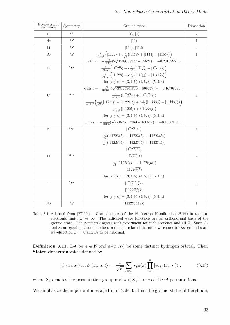
Key ingredients of the PT eigenstates are Slater determinants of the hydrogen orbitals inTable 2.1. Due to their construction, see Definition 3.13, Slater determinants feature thenecessary antisymmetry condition (3.4) for fermions. In physics, [Sch05], and chemistry,[Jen06], Slater determinants are used particularly as ansatz functionals for many-bodysystems such as molecules. For example, the frequently used Hartree-Fock method takesa single Slater determinant and derives, using the Rayleigh-Ritz variational principle7,the ground-state eigenfunction. This method can be applied to any self-adjoint operatorwhich is bounded from below, compare Definition 2.45. However, as Table 3.1 shows, theasymptotic PT ground states are not always given by just a single Slater determinant.This effect occurring for Beryllium, Boron, and Carbon is not described by the Hartree-Fock ansatz as a matter of principle.
For the hydrogen orbitals we recycle the notation |i〉, i = 1, 2, 3, 4, 5, from Table 2.1:from now on, |i〉 denotes the corresponding state with spin “up”, whereas |i〉 denotes thestate with spin “down”.
7We are going to use this method to determine the effective nuclear charge for Lithium later on.
32
3.1 Non-relativistic Perturbation-theory Model
Iso-electronicsequence Symmetry Ground state Dimension
H 2S |1〉, |1〉 2
He 1S |11〉 1
Li 2S |112〉, |112〉 2
Be 1S 1√1+c2
(|1122〉+ c 1√
3
(|1133〉+ |1144〉+ |1155〉
))1
with c = −√
359049
(2√
1509308377− 69821) = −0.2310995 . . .
B 2P o 1√1+c2
(|1122i〉+ c 1√
2
(|11ijj〉+ |11ikk〉
))6
1√1+c2
(|1122i〉+ c 1√
2
(|11ijj〉+ |11ikk〉
))for (i, j, k) = (3, 4, 5), (4, 5, 3), (5, 3, 4)
with c = −√
2393660
(√
733174301809− 809747) = −0.1670823 . . .
C 3P 1√1+c2
(|1122ij〉+ c|11kkij〉
)9
1√1+c2
(1√2
(|1122ij〉+ |1122ij〉
)+ c 1√
2
(|11kkij〉+ |11kkij〉
))1√
1+c2
(|1122ij〉+ c|11kkij〉
)for (i, j, k) = (3, 4, 5), (4, 5, 3), (5, 3, 4)
with c = − 198415
(√
221876564389− 460642) = −0.1056317 . . .
N 4So |1122345〉 4
1√3(|1122345〉+ |1122345〉+ |1122345〉)
1√3(|1122345〉+ |1122345〉+ |1122345〉)
|1122345〉O 3P |1122iijk〉 9
1√2(|1122iijk〉+ |1122iijk〉)
|1122iijk〉for (i, j, k) = (3, 4, 5), (4, 5, 3), (5, 3, 4)
F 2P o |1122iijjk〉 6
|1122iijjk〉for (i, j, k) = (3, 4, 5), (4, 5, 3), (5, 3, 4)
Ne 1S |1122334455〉 1
Table 3.1: Adapted from [FG09b]. Ground states of the N -electron Hamiltonian H(N) in the iso-electronic limit, Z → ∞. The indicated wave functions are an orthonormal basis of theground state. The symmetry agrees with experiment for each sequence and all Z. Since L3
and S3 are good quantum numbers in the non-relativistic setup, we choose for the ground-statewavefunction L3 = 0 and S3 to be maximal.
Definition 3.11. Let be n ∈ N and φi(xi, si) be some distinct hydrogen orbital. TheirSlater determinant is defined by
|φ1(x1, s1) . . . φn(xn, sn)〉 :=1√n!
∑π∈Sn
sgn(π)n∏i=1
|φπ(i)(xi, si)〉 , (3.13)
where Sn denotes the permutation group and π ∈ Sn is one of the n! permutations.
We emphasize the important message from Table 3.1 that the ground states of Beryllium,
33
3 Spectrum of Many-electron Atoms
Boron, and Carbon are not just a single Slater determinant, but some linear combinationof them. We now state one of the main results of the PT model:
Theorem 3.12. For N = 1, . . . , 10 the ground state of H(N) has the spin, angularmomentum, and dimension as given in Table 3.1. In the iso-electronic limit, Z → ∞,its ground state is asymptotic to the indicated vector space in the perturbative sense ofTheorem 3.8.
Proof. This is proven in [FG09b]. Here, we just outline the steps which has to be per-formed in order to derive this result: first of all one has to determine the ground statesV0(N) explicitly. A suitable choice of their bases ensures that the (finite-dimensional) ma-trix PH(N)P is as simple as possible: it obeys block-diagonal form and only some 2× 2matrices must be diagonalized additionally.8 These steps result in an analytic expressionfor the asymptotic eigenstates and energy values.
Remark 3.13. In Table 3.1 we have used the spectroscopic notation for describing thesymmetries of the ground state. In general, 2S+1Xν has the following interpretation: Sdenotes the total spin. The angular momentum, L, corresponds to X via 0↔ S, 1↔ P ,3↔ D, . . . The superscript ν relates to the parity of the state, p = ±1:
ψ(xi, si) = (−1)pψ(−xi, si), simultaneously for all i = 1, . . . , n . (3.14)
If the parity of ψ is odd, i.e. p = −1, the superscript is set to ν = 0. Otherwise, for aneven ψ, p = 1, we suppress the superscript ν.
Example 3.14. The ground-state symmetry of N, N = 7, is labeled by 4S0. This meanstotal spin S = 3/2, total angular momentum L = 0 and odd parity. The ground stateof Oxygen, N = 8, obeys the symmetry 3P , meaning total spin S = 1, total angularmomentum L = 1 and even parity.
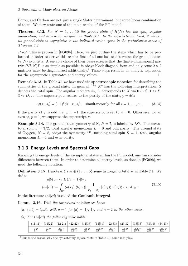
3.1.3 Energy Levels and Spectral Gaps
Knowing the energy levels of the asymptotic states within the PT model, one can considerdifferences between them. In order to determine all energy levels, as done in [FG09b], weneed the following notation:
Definition 3.15. Denote a, b, c, d ∈ 1, . . . , 5 some hydrogen orbital as in Table 2.1. Wedefine
(a|b) := 〈a|H(N = 1)|b〉 ,
(ab|cd) :=
∫R6
〈a(x1)|〈b(x1)| 1
|x1 − x2||c(x2)〉|d(x2)〉 dx1 dx2 .
(3.15)
In the literature (ab|cd) is called the Coulomb integral.
Lemma 3.16. With the introduced notation we have:
(a) (a|b) = δabEn with n = 1 for |a〉 = |1〉, |1〉, and n = 2 in the other cases.
(b) For (ab|cd) the following table holds:
(11|11) (11|22) (12|21) (22|22) (11|33) (13|31) (22|33) (23|32) (33|33) (33|44) (34|43)
58Z 17
81Z 16
729Z 77
512Z 59
243Z 112
6561Z 83
512Z 15
512Z 501
2560Z 447
2560Z 27
2560Z
8This is the reason why the eye-catching square roots in Table 3.1 come into play.
34
3.1 Non-relativistic Perturbation-theory Model
Proof. This can be derived using Fourier analysis. One needs to know the Fourier trans-forms of the functions the hydrogen orbitals consist of. The detailed proof is elaboratedin [FG09b].
Example 3.17. To get used to the very compact notations we now show an explanatorycalculation: we derive the energy of the asymptotic ground state of Lithium, |ψ〉 = |112〉,given in Table 3.1:
〈ψ|H(N = 3)|ψ〉 =
=
⟨1(x1)1(x2)2(x3)
∣∣∣∣∣3∑i=1
(−1
2∆i −
Z
|xi|
)12 +
∑1≤i<j≤3
1
|xi − xj|12
∣∣∣∣∣ 1(x1)1(x2)2(x3)
⟩=
= 3〈1(x1)1(x2)2(x3)|H(1)|1(x1)1(x2)2(x3)〉+ 〈1(x1)1(x2)2(x3)|Vee12|1(x1)1(x2)2(x3)〉 =
= 2E1 + E2 + 〈Vee〉 = −9
8Z2 + 〈Vee〉 ,
where we have used (a|b) = δabEn. Using the even more compact notation 111223 for both,|1(x1)1(x2)2(x3)〉 and 〈1(x1)1(x2)2(x3)|, the interaction between the electrons reads:
〈Vee〉 =
⟨1(x1)1(x2)2(x3)
∣∣∣∣∣ ∑1≤i<j≤3
12
|xi − xj|
∣∣∣∣∣ 1(x1)1(x2)2(x3)
⟩=
=3
3!
∫R9
(111223 − 121123 + 121321 − 131221 + 131122 − 111322)12
|x1 − x2|×
× (111223 − 121123 + 121321 − 131221 + 131122 − 111322) dx1 dx2 dx3 =
=1
2
∫R6
((1112 − 1211)
2+ (1221 − 1222)2 + (1122 − 1221)
2) 1
|x1 − x2|dx1 dx2 =
=1
2
∫R6
((11111212 + 11111212) + (21211212 − 2 · 11212212 + 11112222) +
+ (11112222 + 21211111))1
|x1 − x2|dx1 dx2 = (11|11) + 2(12|21)− (12|21) .
Note that the Coulomb integral is independent of the spin in the following meaning:(aa|bb) = (aa|bb) and (aa|bb) = (aa|bb). Terms like (aa|bb) vanish, since the states withdifferent spin are orthogonal. Using the explicit expressions of the Coulomb integral inLemma 3.16(b), the energy of the asymptotic ground state of Lithium reads
〈112|H(N = 3)|112〉 = −9
8Z2 +
5965
5832Z . (3.16)
The contribution to the energy coming from the interaction between electrons and nucleus,H0(N), can be derived in the general setup of Slater determinants, and, therefore, for allasymptotic states of the PT model:
Lemma 3.18. Denote φi, i = 1, . . . , N , some distinct hydrogen orbitals. One has
〈φ1(x1) . . . φN(xN)|H0(N)|φ1(x1) . . . φN(xN)〉 =N∑i=1
En(i) ,
where we use again n(i) = 1 for |φi〉 = |1〉 and n(i) = 2 in the other cases.
35
3 Spectrum of Many-electron Atoms
Proof. We have to replicate the first part of Example 3.17. For all N ∈ N one gets:
〈φ1(x1) . . . φN(xN)|H0(N)|φ1(x1) . . . φN(xN)〉 =
=1
N !
∑π,σ∈SN
sgn(π)sgn(σ)N∏i=1
⟨φπ(i)(xi)
∣∣∣∣∣N∑k=1
H(1)k
N∏j=1
∣∣∣∣∣φσ(j)(xj)
⟩=
=1
N !
∑π,σ∈SN
sgn(π)sgn(σ)N∏i=1
⟨φπ(i)(xi)
∣∣∣∣∣N∑k=1
En(σ(k))
N∏j=1
∣∣∣∣∣φσ(j)(j)
⟩=
=1
N !
∑π,σ∈SN
sgn(π)sgn(σ)N∑k=1
En(σ(k))
N∏i,j=1
〈φπ(i)(xi)|φσ(j)(xj)〉︸ ︷︷ ︸=δπ,σ
=
=1
N !
∑π∈SN
N∑k=1
En(π(k)) =N∑k=1
En(k) .
In the last step we have used that SN contains N ! elements, which completes the proof.
The structure of the energy of the asymptotic ground state of Li, |112〉, in (3.16) holdsgenerally in the PT model. Combing Lemma 3.16 and Lemma 3.18, we have the generalform of an energy state in the PT model:
E = −|A|Z2 +BZ , (3.17)
where A = A(N) ∈ Q is some negative rational number describing the interaction betweenelectrons and nucleus. For a fixed N = 3, . . . , 10 it is a constant, characteristic for eachchemical element. Besides this, B ∈ R, containing the Coulomb integral, describes theelectron-electron interaction. For all elements of the second shell, B is some positive realnumber, but it depends on the state: ground state (GS or E0), first excited state (E1),second excited state (E2), . . . lead to different values for B. These statements should becompared to the asymptotic states, listed in [FG09b] or in the summary chapter 4.
As a direct consequence of (3.17), the energy gaps within one chemical element, Ei(Z)−Ej(Z), are linear in Z. Due to our perturbative ansatz, we expect our results to agreewith experimental results for large Z → ∞. Therefore, it is convenient to consider thespectral gaps divided by Z2, since this form reads
Ei(Z)− Ej(Z)
Z2= (Bi −Bj)x , (3.18)
which is a straight line in x := 1/Z. Typically, these scaled energies are some meV. Weexpect a good agreement with experimental data for small x→ 0 (⇔ Z →∞). Comparethis to FIG.4(a)-(g) in [FG10].
We derive explicitly the gap between the ground state of Lithium, |112〉, and its firstexcited state |113〉. As done for deriving (3.16) one finds similarly for the first excitedstate: 〈Vee〉 = (11|11) + 2(11|33) − (13|31). The energy term coming from H0(N = 3)is indeed the same as for the ground state. Hence, with the results of Lemma 3.16, theenergy of the first excited state of Lithium reads:
〈113|H(N = 3)|113〉 = −9
8Z2 +
57397
52488Z . (3.19)
36
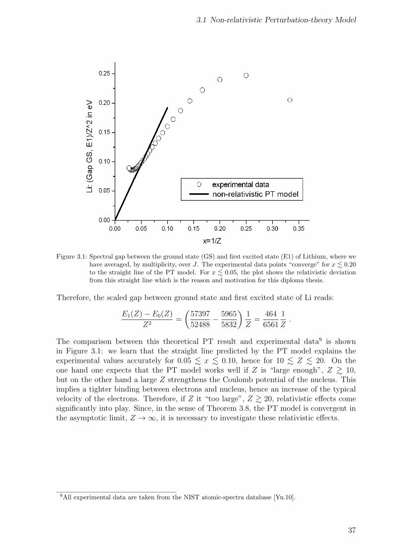
3.1 Non-relativistic Perturbation-theory Model
Figure 3.1: Spectral gap between the ground state (GS) and first excited state (E1) of Lithium, where wehave averaged, by multiplicity, over J . The experimental data points “converge” for x . 0.20to the straight line of the PT model. For x . 0.05, the plot shows the relativistic deviationfrom this straight line which is the reason and motivation for this diploma thesis.
Therefore, the scaled gap between ground state and first excited state of Li reads:
E1(Z)− E0(Z)
Z2=
(57397
52488− 5965
5832
)1
Z=
464
6561
1
Z.
The comparison between this theoretical PT result and experimental data9 is shownin Figure 3.1: we learn that the straight line predicted by the PT model explains theexperimental values accurately for 0.05 . x . 0.10, hence for 10 . Z . 20. On theone hand one expects that the PT model works well if Z is “large enough”, Z & 10,but on the other hand a large Z strengthens the Coulomb potential of the nucleus. Thisimplies a tighter binding between electrons and nucleus, hence an increase of the typicalvelocity of the electrons. Therefore, if Z it “too large”, Z & 20, relativistic effects comesignificantly into play. Since, in the sense of Theorem 3.8, the PT model is convergent inthe asymptotic limit, Z →∞, it is necessary to investigate these relativistic effects.
9All experimental data are taken from the NIST atomic-spectra database [Yu.10].
37
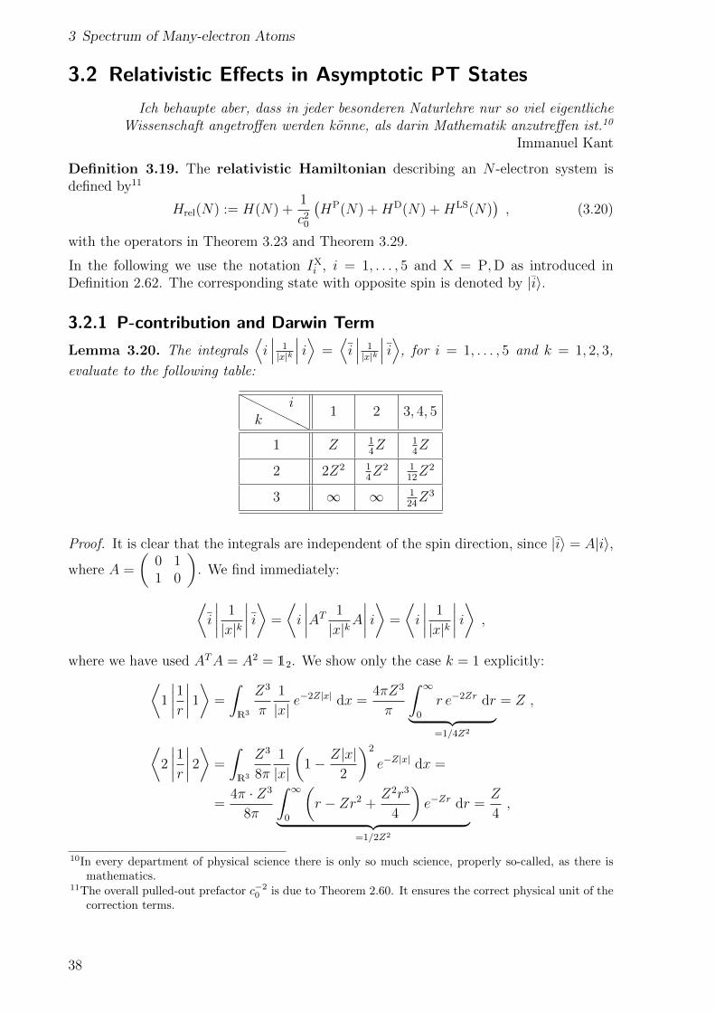
3 Spectrum of Many-electron Atoms
3.2 Relativistic Effects in Asymptotic PT States
Ich behaupte aber, dass in jeder besonderen Naturlehre nur so viel eigentlicheWissenschaft angetroffen werden konne, als darin Mathematik anzutreffen ist.10
Immanuel Kant
Definition 3.19. The relativistic Hamiltonian describing an N -electron system isdefined by11
Hrel(N) := H(N) +1
c20
(HP(N) +HD(N) +HLS(N)
), (3.20)
with the operators in Theorem 3.23 and Theorem 3.29.
In the following we use the notation IXi , i = 1, . . . , 5 and X = P,D as introduced in
Definition 2.62. The corresponding state with opposite spin is denoted by |i〉.
3.2.1 P-contribution and Darwin Term
Lemma 3.20. The integrals⟨i∣∣∣ 1|x|k
∣∣∣ i⟩ =⟨i∣∣∣ 1|x|k
∣∣∣ i⟩, for i = 1, . . . , 5 and k = 1, 2, 3,
evaluate to the following table:
HHHHHHk
i1 2 3, 4, 5
1 Z 14Z 1
4Z
2 2Z2 14Z2 1
12Z2
3 ∞ ∞ 124Z3
Proof. It is clear that the integrals are independent of the spin direction, since |i〉 = A|i〉,where A =
(0 11 0
). We find immediately:
⟨i
∣∣∣∣ 1
|x|k∣∣∣∣ i⟩ =
⟨i
∣∣∣∣AT 1
|x|kA∣∣∣∣ i⟩ =
⟨i
∣∣∣∣ 1
|x|k∣∣∣∣ i⟩ ,
where we have used ATA = A2 = 12. We show only the case k = 1 explicitly:⟨1
∣∣∣∣1r∣∣∣∣ 1⟩ =
∫R3
Z3
π
1
|x| e−2Z|x| dx =
4πZ3
π
∫ ∞0
r e−2Zr dr︸ ︷︷ ︸=1/4Z2
= Z ,
⟨2
∣∣∣∣1r∣∣∣∣ 2⟩ =
∫R3
Z3
8π
1
|x|
(1− Z|x|
2
)2
e−Z|x| dx =
=4π · Z3
8π
∫ ∞0
(r − Zr2 +
Z2r3
4
)e−Zr dr︸ ︷︷ ︸
=1/2Z2
=Z
4,
10In every department of physical science there is only so much science, properly so-called, as there ismathematics.
11The overall pulled-out prefactor c−20 is due to Theorem 2.60. It ensures the correct physical unit of the
correction terms.
38
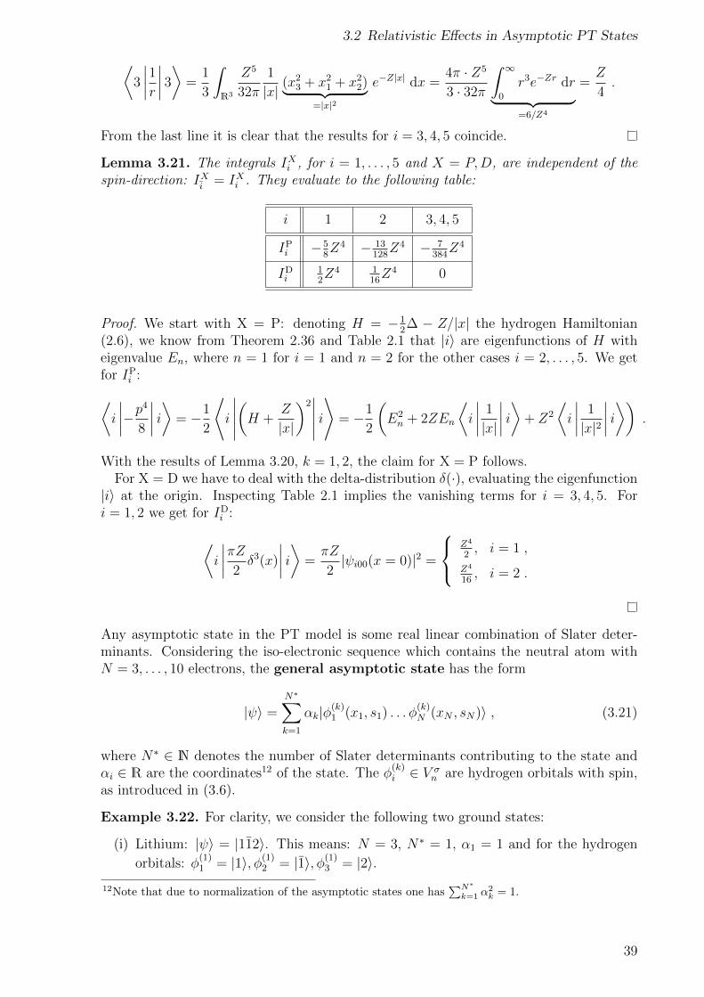
3.2 Relativistic Effects in Asymptotic PT States
⟨3
∣∣∣∣1r∣∣∣∣ 3⟩ =
1
3
∫R3
Z5
32π
1
|x| (x23 + x2
1 + x22)︸ ︷︷ ︸
=|x|2
e−Z|x| dx =4π · Z5
3 · 32π
∫ ∞0
r3e−Zr dr︸ ︷︷ ︸=6/Z4
=Z
4.
From the last line it is clear that the results for i = 3, 4, 5 coincide.
Lemma 3.21. The integrals IXi , for i = 1, . . . , 5 and X = P,D, are independent of thespin-direction: IXi = IXi . They evaluate to the following table:
i 1 2 3, 4, 5
IPi −5
8Z4 − 13
128Z4 − 7
384Z4
IDi
12Z4 1
16Z4 0
Proof. We start with X = P: denoting H = −12∆ − Z/|x| the hydrogen Hamiltonian
(2.6), we know from Theorem 2.36 and Table 2.1 that |i〉 are eigenfunctions of H witheigenvalue En, where n = 1 for i = 1 and n = 2 for the other cases i = 2, . . . , 5. We getfor IP
i :⟨i
∣∣∣∣−p4
8
∣∣∣∣ i⟩ = −1
2
⟨i
∣∣∣∣∣(H +
Z
|x|
)2∣∣∣∣∣ i⟩
= −1
2
(E2n + 2ZEn
⟨i
∣∣∣∣ 1
|x|
∣∣∣∣ i⟩+ Z2
⟨i
∣∣∣∣ 1
|x|2∣∣∣∣ i⟩) .
With the results of Lemma 3.20, k = 1, 2, the claim for X = P follows.For X = D we have to deal with the delta-distribution δ(·), evaluating the eigenfunction|i〉 at the origin. Inspecting Table 2.1 implies the vanishing terms for i = 3, 4, 5. Fori = 1, 2 we get for ID
i :
⟨i
∣∣∣∣πZ2 δ3(x)
∣∣∣∣ i⟩ =πZ
2|ψi00(x = 0)|2 =
Z4
2, i = 1 ,
Z4
16, i = 2 .
Any asymptotic state in the PT model is some real linear combination of Slater deter-minants. Considering the iso-electronic sequence which contains the neutral atom withN = 3, . . . , 10 electrons, the general asymptotic state has the form
|ψ〉 =N∗∑k=1
αk|φ(k)1 (x1, s1) . . . φ
(k)N (xN , sN)〉 , (3.21)
where N∗ ∈ N denotes the number of Slater determinants contributing to the state andαi ∈ R are the coordinates12 of the state. The φ
(k)i ∈ V σ
n are hydrogen orbitals with spin,as introduced in (3.6).
Example 3.22. For clarity, we consider the following two ground states:
(i) Lithium: |ψ〉 = |112〉. This means: N = 3, N∗ = 1, α1 = 1 and for the hydrogen
orbitals: φ(1)1 = |1〉, φ(1)
2 = |1〉, φ(1)3 = |2〉.
12Note that due to normalization of the asymptotic states one has∑N∗
k=1 α2k = 1.
39
3 Spectrum of Many-electron Atoms
(ii) Beryllium: |ψ〉 = 1√1+c2
(|1122〉+ c√
3(|1133〉+ |1144〉+ |1155〉)
). This more com-
plicated state implies: N = 4, N∗ = 4, α1 = 1√1+c2
, α2 = α3 = α4 = c√3√
1+c2
and φ(k)1 = |1〉, φ(k)
2 = |1〉 for all k = 1, . . . , 4. Furthermore φ(1)3 = |2〉, φ(1)
4 = |2〉,φ
(2)3 = |3〉, φ(2)
4 = |3〉, φ(3)3 = |4〉, φ(3)
4 = |4〉 and φ(4)3 = |5〉, φ(4)
4 = |5〉.
Theorem 3.23. Let be X = P,D with the corresponding operators13:
HP (N) :=N∑i=1
HPi = −
N∑i=1
p4i
8and HD(N) :=
N∑i=1
HDi =
πZ
2
N∑i=1
δ(3)(xi) , (3.22)
where the subscript i tells us that the operator HXi acts only on the i-th electron. Then,
the relativistic correction to the general asymptotic state, |ψ〉 in (3.21), is given by
〈ψ|HX(N)|ψ〉 =N∗∑k=1
α2k
N∑i=1
IX∣∣∣φ(k)i
⟩ . (3.23)
Proof. Using the orthogonality of the hydrogen orbitals, 〈i|j〉 = δij, we get:
〈ψ|HX(N)|ψ〉 =N∗∑k=1
N∗∑l=1
αkαl〈φ(k)1 (x1) . . . φ
(k)N (xN)|HX |φ(l)
1 (x1) . . . φ(l)N (xN)〉 =
=N∗∑k=1
α2k〈φ(k)
1 (x1) . . . φ(k)N (xN)|HX |φ(k)
1 (x1) . . . φ(k)N (xN)〉 =
=N
N !
N∗∑k=1
α2k
∑π,σ∈SN
sgn(π)sgn(σ)N∏i=1
⟨ψ
(k)π(i)(xi)
∣∣∣∣∣HX1
N∏j=1
∣∣∣∣∣φ(k)σ(j)(xj)
⟩︸ ︷︷ ︸
=δπ,σIX|φ(k)π(1)〉
.
Besides the orthogonality we have used that all terms of HX =∑N
i=1HXi contribute in the
same way, hence the global prefactor N has arosen. Now, δπ,σ removes one of the sums
over the permutation group. Inserting a decomposition of the identity, 1 =∑N
i=1 δi,π(1),restricts the π-sum to the subgroup SN−1, hence we have
〈ψ|HX(N)|ψ〉 =1
(N − 1)!
N∗∑k=1
α2k
∑π∈SN
IX∣∣∣φ(k)π(1)
⟩ =
=1
(N − 1)!
N∗∑k=1
α2k
N∑i=1
∑π∈SN
δi,π(1)︸ ︷︷ ︸π∈SN−1
IX∣∣∣φ(k)i
⟩ =N∗∑k=1
α2k
N∑i=1
IX∣∣∣φ(k)i
⟩ .
In the last step we have used that IX∣∣∣φ(k)i
⟩ is independent of the permutation π.
13These operators are direct N -electron generalizations of the correction terms in Definition 2.62. ForN = 1 they restore to 〈i|HX |i〉 = IXi .
40
3.2 Relativistic Effects in Asymptotic PT States
3.2.2 Spin-orbit Coupling
Now we investigate the relativistic correction induced by the spin: the LS-coupling. Forthe beginning we restrict to the one-particle operators L(k) and S(k). We know alreadythat in a relativistic setup the operators L(k) and S(k) are no conserved quantities,Lemma 3.5(b), hence they are no longer appropriate. Instead, we have introduced thetotal angular momentum J(k) = L(k) + S(k) which is a good quantum number for theDirac operator. In the non-relativistic setup, additionally L3(k) and S3(k) commute withthe Hamiltonian. Since we are restricted to the second shell, and |1〉 and |2〉 featurel = 0, we need to consider only hydrogen orbitals with l = 1, i.e. |i〉 for i = 3, 4, 5. Theeigenvalue equations read L2ψσnlm = l(l + 1)ψσnlm and S2ψσnlm = 3
4ψσnlm.
In addition, due to [Si(k), S2(k)] = 0 for all i = 1, 2, 3, ψσnlm are also eigenfunctionsof one14 component of S(k). This statement is also true for the angular-momentumoperator: one component of L(k) is diagonal in the basis formed by ψσnlm. We follow theusual convention and choose L3 and S3 to be the diagonal ones. Also for these operators,we know the eigenvalues: L3ψ
σnlm = mψσnlm, for m = −l, . . . , l, compare (A.20), and
S3ψσnlm = ±1
2ψσnlm.
Since electrons have spin 1/2, the Clebsch-Gordan decomposition yields (for l ≥ 1) onlytwo components: j = l− 1
2and j = l+ 1
2. The eigenfunction of J2(k) are denoted by |j±〉.
Note that the multiplicities of j = l− 12
and j = l+ 12
sum up to 2(l− 12)+1+2(l+ 1
2)+1 =
4l + 2, as expected from the multiplicity of the product state of spin 12
and angularmomentum l: 2 · (2l + 1) = 4l + 2.
Lemma 3.24. For the two one-particle states |j±〉 the following eigenvalue equationshold:
L · S|j+〉 =l
2|j+〉 , and L · S|j−〉 = − l + 1
2|j−〉 . (3.24)
Proof. Knowing from the above discussion that |j±〉 are eigenstates of J2, L2 and S2, weget directly:
L · S|j±〉 =1
2
(J2 − L2 − S2
)|j±〉 =
=1
2
((l ± 1
2
)(l ± 1
2+ 1
)− l(l + 1)− 3
4
)|j±〉 =
l2|j+〉, j = l + 1
2,
− l+12|j−〉, j = l − 1
2.
From this we are able to derive the energy corrections for the two possible J-states whencoupling the spin of one electron to its angular momentum:
Lemma 3.25. Let be n = 2, l = 1 and i = 3, 4, 5. We define |i±〉 := |i, j = l ± 12〉. With
this, we derive
I± :=
⟨i±∣∣∣∣Z2 L · S|x|3
∣∣∣∣ i±⟩ =
196Z4, j = 3
2,
− 148Z4, j = 1
2.
14In fact, since the commutator of the Pauli matrices σi is non trivial, [σi, σj ] = 2iεijkσk, it is impossibleto find a basis in which all three components of the angular-momentum operator S(k) are diagonal.Compare Appendix A.3, where we define the totally anti-symmetric ε tensor.
41
3 Spectrum of Many-electron Atoms
Proof. We only have to combine Lemma 3.21 and Lemma 3.24. We consider only thestate |i+〉 for i = 3, 4, 5:
I+ =
⟨i+
∣∣∣∣ 1
|x|3L · S∣∣∣∣ i+⟩ =
l
2
⟨i+
∣∣∣∣ 1
|x|3∣∣∣∣ i+⟩ =
lZ3
48.
Multiplying by Z/2 yields for l = 1 our claim. Similarly the claim follows for |i−〉.
When considering an N -electron state with angular momentum L and spin S, the Clebsch-Gordan decomposition contains L+S− |L−S|+ 1 terms. The total angular momentumJ can be J = |L−S|, |L−S|+1, . . . , L+S, which is known as the triangular condition.Note that for a one-particle state, angular momentum l = 1 and spin 1/2, the two termsj = 1/2 and j = 3/2, appear as a special case. We introduce the following notation:
Definition 3.26.
(i) N+ denotes the number of electrons with spin “up”, N− those with spin “down”:
N± = 0, . . . , N, with N+ +N− = N .
(ii) For a general asymptotic state, |ψ〉 in (3.21), we denote by N∗k , k = 1, . . . , N∗, thenumbers of l 6= 0−orbitals in the k-th term:
N∗k := #|i〉, |i〉, i = 3, 4, 5, in |φ(k)
1 . . . φ(k)N 〉.
Example 3.27. For the two states in Example 3.22 we have for Li: N∗1 = 1. For Be wehave: N∗1 = 0 and N∗2 = N∗3 = N∗4 = 2.
Remark 3.28. For a given angular momentum, L = 0, 1, 2, . . ., and total angular mo-mentum, J = 0, 1
2, 1, 3
2, 2, . . ., of an N -electron state, the spin configuration must obey:
J!
= |L+1
2N+ − 1
2N−| = |L+
N
2−N−| , for N− = 1, . . . , N − 1 . (3.25)
Due to the closed first shell, n = 1 with |1〉 and |1〉, the number of electrons with “spin up”and “spin down” is at least one in both cases. Since the PT model restricts to the secondshell, N = 3, . . . , 10, we have always N± = 1, 2, . . . , N − 1. However, it will turn outthat there are for some combinations of L, J and N two possible values for N− satisfying(3.25), particularly for Carbon, Nitrogen, Oxygen and Fluorine.
Corresponding to Theorem 3.23 for X = P,D, we are now able to state in Theorem 3.29the relativistic corrections which are induced by the spin-orbit coupling. The operatorHLSi defined therein takes only the diagonal term of the whole LS-correction into account:
L · S =
(N∑k=1
L(k)
)·(
N∑k=1
S(k)
)=
N∑k=1
L(k) · S(k) +∑
1≤k<k′≤N
L(k) · S(k′) . (3.26)
We justify the restriction to the diagonal contributions as follows: the ground statesthe relativistic corrections are derived for are given in Table 3.1, the first excited statescan be found in [FG09b]. All these PT states are derived using perturbation theorywith respect to the Coulomb interaction between different electrons. The asymptotic
42
3.2 Relativistic Effects in Asymptotic PT States
ground states become exact solutions of the Schrodinger equation for Z →∞, where theelectron-nucleus interaction becomes more and more dominant. Therefore it is consistentto take off also the electromagnetic interaction between different electrons when discussingrelativistic effects of the asymptotic states. By the local model we denote the restrictionto the diagonal term of L·S and tracing back the spin-orbit coupling to each single electronand its own j-state. Compare this to the discussion in section 3.6 and also Remark 3.32.
Theorem 3.29. Let HLS(N) denote the N-particle spin-orbit operator, defined by15
HLS(N) :=N∑i=1
HLSi =
Z
2
N∑i=1
L(i) · S(i)
|xi|3, (3.27)
where the subscript i tells us that the operator HLSi acts only on the i-th electron. Let
the general asymptotic state, |ψ〉 in (3.21), have the total angular momentum J , denotedby |ψ〉J . The spin structure is described by the two parameters N± and the coefficientsN∗k . Then, for the chemical elements in the second shell, N = 3, . . . , 10, the relativisticcorrection induced by the local spin-orbit coupling reads:
〈ψ|HLS(N)|ψ〉J =Z4
96
N + 1− 3N−
N − 2
N∗∑k=1
α2kN∗k . (3.28)
Proof. As in the proof of Theorem 3.23 we use the orthogonality of the hydrogen states,hence the orthogonality of the J2-eigenstates |i±〉:
〈ψ|HLS(N)|ψ〉J =N∗∑k=1
α2k
N∑i=1
1
N−2
(N+
⟨φ
(k)i +
∣∣∣∣Z2 L·S|x|3∣∣∣∣φ(k)
i +
⟩+N−
⟨φ
(k)i −
∣∣∣∣Z2 L·S|x|3∣∣∣∣φ(k)
i −⟩)
.
From Lemma 3.25 we know that only the l 6= 0−orbitals have a non-trivial contribution.Additionally, this contribution is independent of the explicit state |i±〉, i = 3, 4, 5, hencewe find N∗k identical terms:
〈ψ|HLS(N)|ψ〉J =N∗∑k=1
α2kN∗k
(N+ − 1)I+ + (N− − 1)I−N − 2
=Z4
96
N + 1− 3N−
N − 2
N∗∑k=1
α2kN∗k ,
where we have used the explicit expressions for ILS± and ILS− = −2ILS+ . Note that theterms (N± − 1)/(N − 2) appear due to the closed first shell: for all N = 3, . . . , 10, thereare two electrons in the first shell, |1〉 and |1〉, with opposite spin direction. The otherN − 2 electron spins together with their angular momenta have to sum up to the totalangular momentum J .
Corollary 3.30. The sign of the LS-correction (3.28) depends only on N±:
sgn 〈ψ|HLS(N)|ψ〉J = sgn(N + 1− 3N−
)= sgn
(N+ + 1
N−− 2
). (3.29)
Particularly, the spin does not affect the energy levels ⇔ 3N− = N + 1.
15Note that the operator∑
i L(i)S(i) commutes with both the non-relativistic N -particle Hamiltonian,H(N), and the PT-Hamiltonian, PH(N)P .
43
3 Spectrum of Many-electron Atoms
Remark 3.31. Since we are restricted to the second shell, N = 3, . . . , 10, only for energystates of Boron, N = 5, or Oxygen, N = 8, it is possible that the spin-orbit couplingimplies finally no relativistic correction.
3.2.3 Relativistic Energy Levels, Spectral Gaps and Splitting
We conclude briefly the general form of an energy state in the relativistic PTmodel: combining Theorem 3.23 and Theorem 3.29, we find the relativistic generalizationof (3.17):
E = −|A|Z2 +BZ +C
c20
Z4 , (3.30)
with A and B are as above and C ∈ Q. The relativistic parameter C can be both, positiveor negative. (3.30) implies a deviation also of the Z2-scaled spectral gaps (3.18):
EJii (Z)− EJj
j (Z)
Z2= (Bi −Bj)x+
1
c20
(CJii − C
Jjj
) 1
x2=: ∆Bx+
∆C
c20
1
x2, (3.31)
where we have defined x := 1/Z. The J-independent constant ∆B is known from the non-relativistic PT model, whereas ∆C must be derived using the results we have preparedin this section. If ∆C > 0, then the straight line predicted by the non-relativistic PTmodel is shifted upwards for x→ 0 (⇔ Z →∞). In the other case, ∆C < 0, the shift isdownwards.
Additionally, the relativistic corrections feature a splitting of the asymptotic PT states:in general, different values of J cause different shifts of the energy states. It is convenientto consider the splittings divided by Z5:
EJi(Z)− EJj(Z)
Z5=
∆C
c20
x , (3.32)
which is again a straight line in x = 1/Z. Typically, due to the high power of Z, thesescaled energies are only a few µeV.
Remark 3.32. The form of the energy E(Z) in (3.30) shows that the relativistic cor-rection, ∼ Z4, becomes the dominant contribution to the energy in the asymptotic limitZ →∞. But this is the limit we need the asyptotic states to be close to the Schrodingerstates. For the comparison to experimental data this implies that one can expect to findan agreement to the local model for large, but not too large values of Z. Since there isonly a finite number of ions in each iso-electronic sequence experimentally available, theprecedure we are doing is still reasonable. However, for Z → ∞ perturbation theory atfirst order in the relativistic sector is physically not sufficient: higher order correctionsbecome more important since they feature an even higher power of Z.
44
3.3 Relativistic Corrections to Lithium
3.3 Relativistic Corrections to Lithium
Die Physik erklart die Geheimnisse der Natur nicht,sie fuhrt sie auf tieferliegende Geheimnisse zuruck.16
Carl Friedrich von Weizsacker
In this section we derive in detail the relativistic corrections to the asymptotic states ofLithium-like ions17, N = 3, of the PT model. We will apply the general considerationsof the local model to the ground state, ψ0 = |112〉, and first excited state, ψ1 = |113〉,derived in [FG09b].
For the energy corrections18 we use the following notation: ∆EJi denotes the total
correction of the ground state, i = 0, or first excited state, i = 1, with total angularmomentum J . If there is only one possible J , i.e. L or S vanish, we suppress thesuperscript J . The J-independent corrections, P-contribution and Darwin term, sum upto ∆EP+D
i := ∆EPi + ∆ED
i . The J-dependent spin-orbit correction is denoted by ∆ELS,Ji .
3.3.1 Shifted Energy Levels
We start with the asymptotic ground state of Li: ψ0 = |112〉 with L = 0, S = 1/2, henceJ = 1/2. Theorem 3.23 tells us how its relativistic correction due to the P-contributionand the Darwin term reads:
∆EP+D0 = 2IP
1 + IP2 + 2ID
1 + ID2 = − 37
128Z4 , (3.33)
where we have used the explicit expression of Lemma 3.21. Due to L = 0, particularlyN∗1 = 0, the ground state does not have any spin-correction, hence ∆E0 = ∆EP+D
0 .The first excited state of Li, |113〉 has L = 1 and S = 1/2, hence there are two possible
total angular momenta: J = 1/2, 3/2. The J-independent corrections reads:
∆EP+D1 = 2IP
1 + IP3 + 2ID
1 = −103
384Z4 . (3.34)
For the spin-orbit corrections, we apply Theorem 3.29. The spin structure, described byN±, must obey (3.25): for J = 1/2 we get N+ = 1 and N− = 2, for J = 3/2 we getN+ = 2 and N− = 1. This yields
∆ELS,1/21 = − 1
48Z4 and ∆E
LS,3/21 =
1
96Z4 . (3.35)
Proposition 3.33. The relativistic corrections to the ground state, |112〉, and first excitedstate, |113〉, of Lithium are given by:
∆E0 = − 37
128Z4 , ∆E
1/21 = − 37
128Z4 , ∆E
3/21 = − 33
128Z4 .
In particular one has the degeneracy ∆E0 = ∆E1/21 . The shifted energy levels are sketched
in Figure 3.2, and the comparison to experimental data is shown in Figure 3.3.
16Physics does not explain the secrets of nature, it traces nature back to more fundamental secrets.17We will drop this cumbersome notation and denote it just by the term “Lithium”.18Note that there is a global prefactor of c−2
0 coming from the definition of the relativistic Hamiltonian(3.20). When evaluating to numbers (in atomic units), we need to divide our results by c20 ≈ 1372.
45
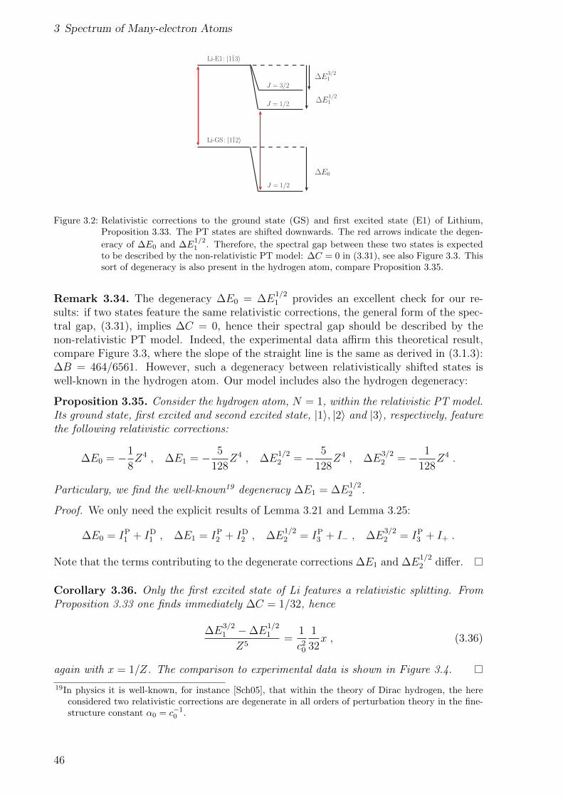
3 Spectrum of Many-electron Atoms
Li-E1 : |113〉
Li-GS: |112〉
J = 3/2
J = 1/2
J = 1/2
ΔE3/21
ΔE1/21
ΔE0
Figure 3.2: Relativistic corrections to the ground state (GS) and first excited state (E1) of Lithium,Proposition 3.33. The PT states are shifted downwards. The red arrows indicate the degen-
eracy of ∆E0 and ∆E1/21 . Therefore, the spectral gap between these two states is expected
to be described by the non-relativistic PT model: ∆C = 0 in (3.31), see also Figure 3.3. Thissort of degeneracy is also present in the hydrogen atom, compare Proposition 3.35.
Remark 3.34. The degeneracy ∆E0 = ∆E1/21 provides an excellent check for our re-
sults: if two states feature the same relativistic corrections, the general form of the spec-tral gap, (3.31), implies ∆C = 0, hence their spectral gap should be described by thenon-relativistic PT model. Indeed, the experimental data affirm this theoretical result,compare Figure 3.3, where the slope of the straight line is the same as derived in (3.1.3):∆B = 464/6561. However, such a degeneracy between relativistically shifted states iswell-known in the hydrogen atom. Our model includes also the hydrogen degeneracy:
Proposition 3.35. Consider the hydrogen atom, N = 1, within the relativistic PT model.Its ground state, first excited and second excited state, |1〉, |2〉 and |3〉, respectively, featurethe following relativistic corrections:
∆E0 = −1
8Z4 , ∆E1 = − 5
128Z4 , ∆E
1/22 = − 5
128Z4 , ∆E
3/22 = − 1
128Z4 .
Particulary, we find the well-known19 degeneracy ∆E1 = ∆E1/22 .
Proof. We only need the explicit results of Lemma 3.21 and Lemma 3.25:
∆E0 = IP1 + ID
1 , ∆E1 = IP2 + ID
2 , ∆E1/22 = IP
3 + I− , ∆E3/22 = IP
3 + I+ .
Note that the terms contributing to the degenerate corrections ∆E1 and ∆E1/22 differ.
Corollary 3.36. Only the first excited state of Li features a relativistic splitting. FromProposition 3.33 one finds immediately ∆C = 1/32, hence
∆E3/21 −∆E
1/21
Z5=
1
c20
1
32x , (3.36)
again with x = 1/Z. The comparison to experimental data is shown in Figure 3.4.
19In physics it is well-known, for instance [Sch05], that within the theory of Dirac hydrogen, the hereconsidered two relativistic corrections are degenerate in all orders of perturbation theory in the fine-structure constant α0 = c−1
0 .
46
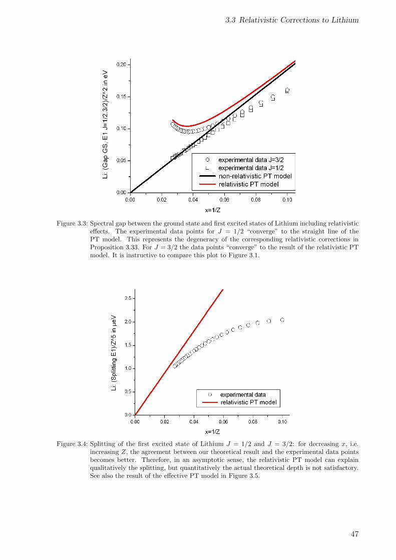
3.3 Relativistic Corrections to Lithium
Figure 3.3: Spectral gap between the ground state and first excited states of Lithium including relativisticeffects. The experimental data points for J = 1/2 “converge” to the straight line of thePT model. This represents the degeneracy of the corresponding relativistic corrections inProposition 3.33. For J = 3/2 the data points “converge” to the result of the relativistic PTmodel. It is instructive to compare this plot to Figure 3.1.
Figure 3.4: Splitting of the first excited state of Lithium J = 1/2 and J = 3/2: for decreasing x, i.e.increasing Z, the agreement between our theoretical result and the experimental data pointsbecomes better. Therefore, in an asymptotic sense, the relativistic PT model can explainqualitatively the splitting, but quantitatively the actual theoretical depth is not satisfactory.See also the result of the effective PT model in Figure 3.5.
47
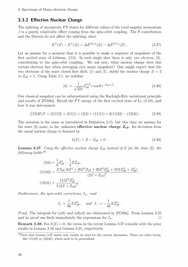
3 Spectrum of Many-electron Atoms
3.3.2 Effective Nuclear Charge
The splitting of asymptotic PT states for different values of the total angular momentumJ is a purely relativistic effect coming from the spin-orbit coupling. The P-contributionand the Darwin do not affect the splitting, since
EJi(Z)− EJj(Z) = ∆ELS,Ji(Z)−∆ELS,Jj(Z) . (3.37)
Let us assume for a moment that it is possible to make a sequence of snapshots of thefirst excited state of Lithium, |113〉. In each single shot there is only one electron, |3〉,contributing to the spin-orbit coupling. We ask now, what nuclear charge does thiscertain electron face when averaging over many snapshots? One might expect that thetwo electrons of the inner closed first shell, |1〉 and |1〉, shield the nuclear charge Z = 3to Zeff = 1. Using Table 2.1, we redefine
|3〉 :=1√32π
Z5/2eff r cos θ e−Zeffr/2 . (3.38)
Our classical snapshot can be substantiated using the Rayleigh-Ritz variational principleand results of [FG09a]. Recall the PT energy of the first excited state of Li, (3.19), andhow it was determined:
〈113|H(N = 3)|113〉 = 2(1|1) + (3|3) + (11|11) + 2(11|33)− (13|31) . (3.39)
The notation is the same as introduced in Definition 3.15, but this time we assume forthe state |3〉 some, so far, unknown effective nuclear charge Zeff . Its deviation fromthe usual nuclear charge is denoted by
δ(Z) := Z − Zeff > 0 . (3.40)
Lemma 3.37. Using the effective nuclear charge Zeff instead of Z for the state |3〉, thefollowing holds:20
(3|3) =1
8Z2
eff −1
4ZZeff ,
(11|33) =ZZeff (8Z4 + 20Z3Zeff + 20Z2Z2
eff + 10ZZ3eff + Z4
eff)
(2Z + Zeff)5 ,
(13|31) =112Z3Z5
eff
3 (2Z + Zeff)7 .
Furthermore, the spin-orbit corrections, I±, read
I+ =1
96ZZ3
eff , and I− = − 1
48ZZ3
eff .
Proof. The integrals for (a|b) and (ab|cd) are elaborated in [FG09a]. From Lemma 3.25and its proof one finds immediately the expressions for I±.
Remark 3.38. For δ(Z) = 0, the terms in the recent Lemma 3.37 coincide with the priorresults in Lemma 3.16 and Lemma 3.25, respectively.
20Note that Lemma 3.37 states only results we need for the current discussion. There are other terms,like (11|33) or (23|32), which need to be generalized.
48
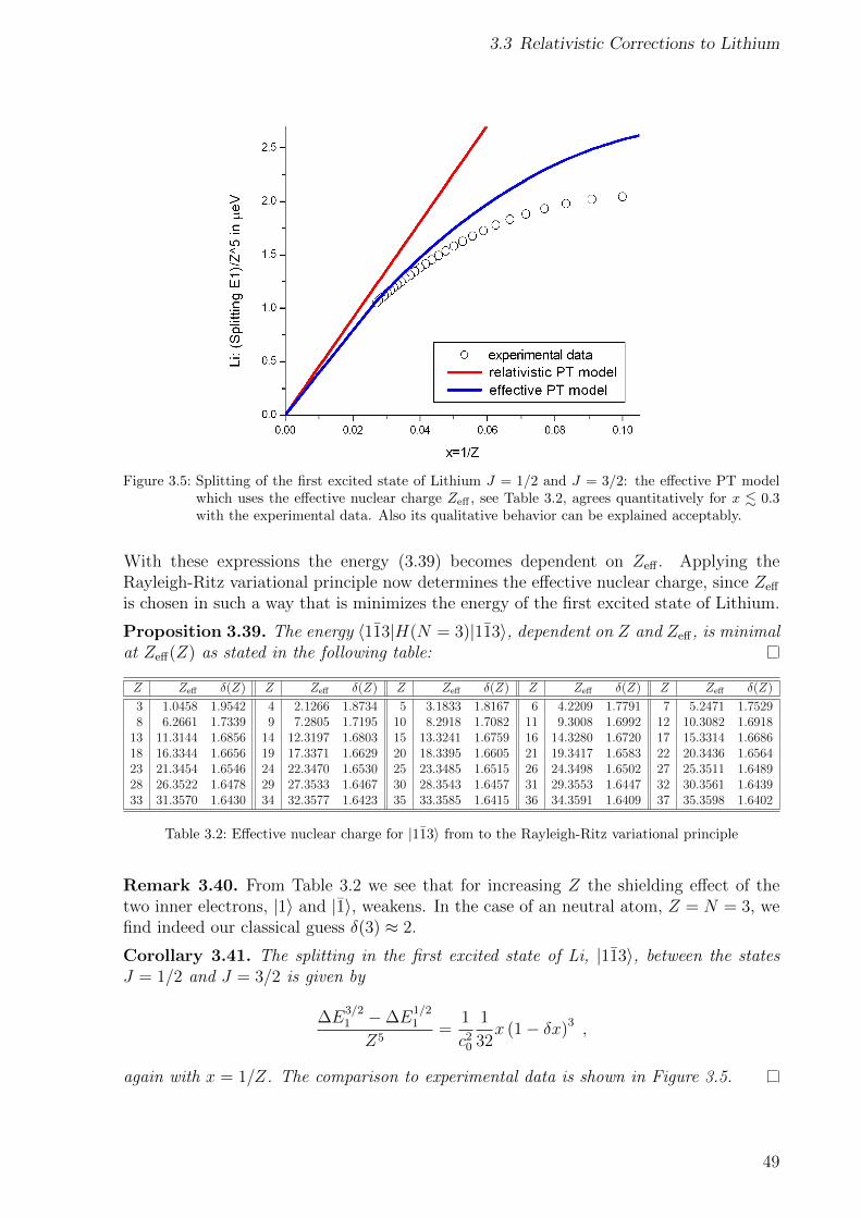
3.3 Relativistic Corrections to Lithium
Figure 3.5: Splitting of the first excited state of Lithium J = 1/2 and J = 3/2: the effective PT modelwhich uses the effective nuclear charge Zeff , see Table 3.2, agrees quantitatively for x . 0.3with the experimental data. Also its qualitative behavior can be explained acceptably.
With these expressions the energy (3.39) becomes dependent on Zeff . Applying theRayleigh-Ritz variational principle now determines the effective nuclear charge, since Zeff
is chosen in such a way that is minimizes the energy of the first excited state of Lithium.
Proposition 3.39. The energy 〈113|H(N = 3)|113〉, dependent on Z and Zeff , is minimalat Zeff(Z) as stated in the following table:
Z Zeff δ(Z) Z Zeff δ(Z) Z Zeff δ(Z) Z Zeff δ(Z) Z Zeff δ(Z)
3 1.0458 1.9542 4 2.1266 1.8734 5 3.1833 1.8167 6 4.2209 1.7791 7 5.2471 1.75298 6.2661 1.7339 9 7.2805 1.7195 10 8.2918 1.7082 11 9.3008 1.6992 12 10.3082 1.6918
13 11.3144 1.6856 14 12.3197 1.6803 15 13.3241 1.6759 16 14.3280 1.6720 17 15.3314 1.668618 16.3344 1.6656 19 17.3371 1.6629 20 18.3395 1.6605 21 19.3417 1.6583 22 20.3436 1.656423 21.3454 1.6546 24 22.3470 1.6530 25 23.3485 1.6515 26 24.3498 1.6502 27 25.3511 1.648928 26.3522 1.6478 29 27.3533 1.6467 30 28.3543 1.6457 31 29.3553 1.6447 32 30.3561 1.643933 31.3570 1.6430 34 32.3577 1.6423 35 33.3585 1.6415 36 34.3591 1.6409 37 35.3598 1.6402
Table 3.2: Effective nuclear charge for |113〉 from to the Rayleigh-Ritz variational principle
Remark 3.40. From Table 3.2 we see that for increasing Z the shielding effect of thetwo inner electrons, |1〉 and |1〉, weakens. In the case of an neutral atom, Z = N = 3, wefind indeed our classical guess δ(3) ≈ 2.
Corollary 3.41. The splitting in the first excited state of Li, |113〉, between the statesJ = 1/2 and J = 3/2 is given by
∆E3/21 −∆E
1/21
Z5=
1
c20
1
32x (1− δx)3 ,
again with x = 1/Z. The comparison to experimental data is shown in Figure 3.5.
49
3 Spectrum of Many-electron Atoms
3.4 Relativistic Corrections to Beryllium, Boron andCarbon
Wer nichts als Chemie versteht, versteht auch die nicht recht.21
Georg Christoph Lichtenberg
The ground state of Beryllium is the first PT state which is not just a single Slaterdeterminant, but a sum of four Slater determinants, see Table 3.1 for the asymptoticground states, L3 = 0 and S3 is maximal:
ψBe0 =
1√1 + c2
(|1122〉+
c√3
(|1133〉+ |1144〉+ |1155〉)), (3.41)
with
c = −√
3
59049
(2√
1509308377− 69821)≈ −0.23 . (3.42)
The dominant term, |1122〉, contributes with almost 95%. The quantum numbers of ψBe0
read L = 0 and S = 0, hence only J = 0 is possible. For the P-contribution and theDarwin term we find:
∆EP+D0 =
2
1 + c2
(IP
1 + IP2 + ID
1 + ID2
)+
2c2
1 + c2
(IP
1 + IP3 + ID
1
)=
= − 1
1 + c2
(21
64+ c2 55
192
)Z4 .
(3.43)
The spin-structure reads N+ = N− = 2, hence
∆ELS0 = − c2
1 + c2
1
94Z4 . (3.44)
The first excited state of Be with quantum numbers L = 1 and S = 1 reads much easier:
ψBe1 := |1123〉 . (3.45)
For the P-contribution and the Darwin term we find we find immediately:
∆EP+D1 = 2
(IP
1 + ID1
)+ IP
2 + ID2 + IP
3 = − 59
192Z4 . (3.46)
There are three possible total angular momenta: J = 0 (N+ = 1, N− = 3), J = 1(N+ = 2, N− = 2), or J = 2 (N+ = 3, N− = 1).
Proposition 3.42. The relativistic corrections to the ground state, ψBe0 , and first excited
state, ψBe1 , of Beryllium are given by:
∆E0 = − 1
1 + c2
(21
64+ c2 19
64
)Z4 ,
∆E01 = −21
64Z4 , ∆E1
1 = −20
64Z4 , ∆E2
1 = −19
64Z4 ,
where c is given in (3.42).
21He who understands nothing but chemistry does not truly understand chemistry either.
50
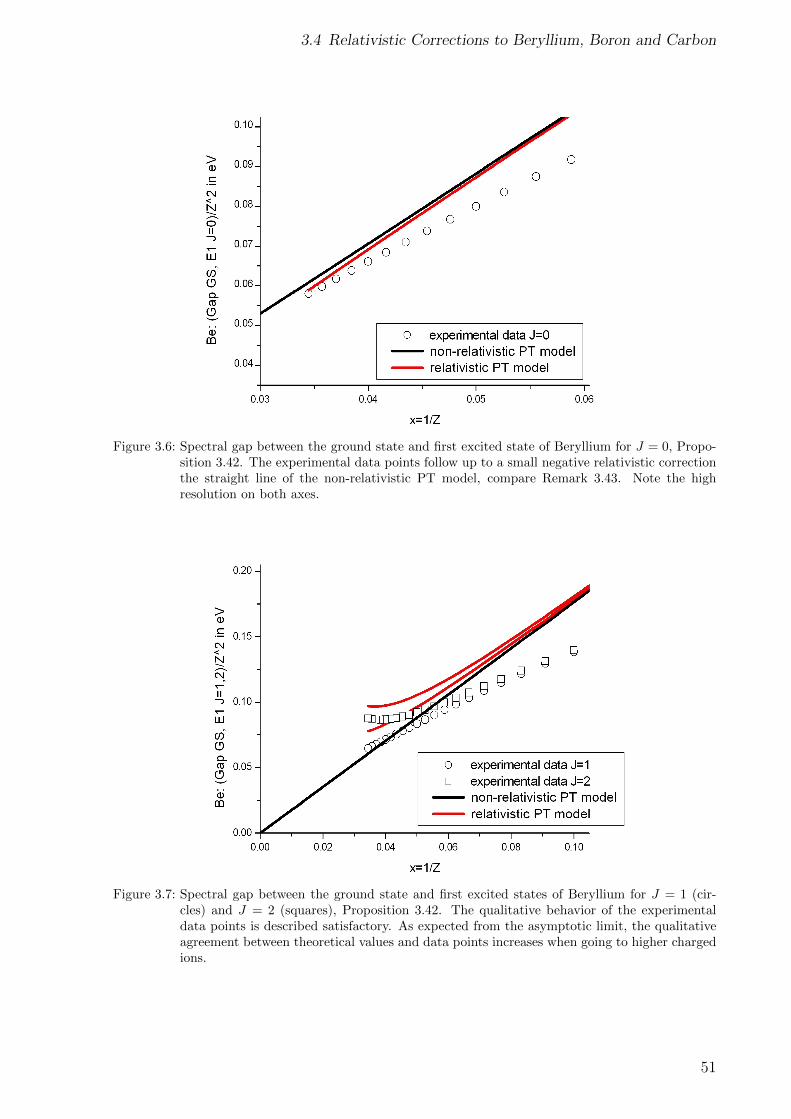
3.4 Relativistic Corrections to Beryllium, Boron and Carbon
Figure 3.6: Spectral gap between the ground state and first excited state of Beryllium for J = 0, Propo-sition 3.42. The experimental data points follow up to a small negative relativistic correctionthe straight line of the non-relativistic PT model, compare Remark 3.43. Note the highresolution on both axes.
Figure 3.7: Spectral gap between the ground state and first excited states of Beryllium for J = 1 (cir-cles) and J = 2 (squares), Proposition 3.42. The qualitative behavior of the experimentaldata points is described satisfactory. As expected from the asymptotic limit, the qualitativeagreement between theoretical values and data points increases when going to higher chargedions.
51
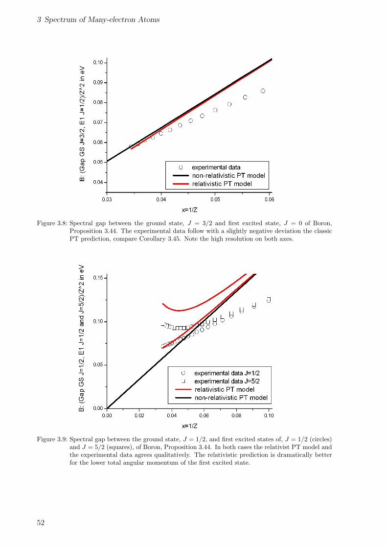
3 Spectrum of Many-electron Atoms
Figure 3.8: Spectral gap between the ground state, J = 3/2 and first excited state, J = 0 of Boron,Proposition 3.44. The experimental data follow with a slightly negative deviation the classicPT prediction, compare Corollary 3.45. Note the high resolution on both axes.
Figure 3.9: Spectral gap between the ground state, J = 1/2, and first excited states of, J = 1/2 (circles)and J = 5/2 (squares), of Boron, Proposition 3.44. In both cases the relativist PT model andthe experimental data agrees qualitatively. The relativistic prediction is dramatically betterfor the lower total angular momentum of the first excited state.
52
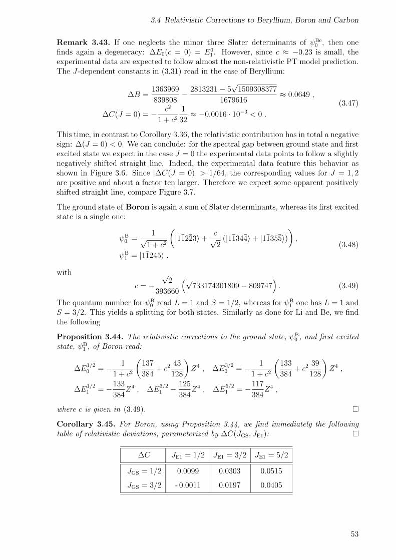
3.4 Relativistic Corrections to Beryllium, Boron and Carbon
Remark 3.43. If one neglects the minor three Slater determinants of ψBe0 , then one
finds again a degeneracy: ∆E0(c = 0) = E01 . However, since c ≈ −0.23 is small, the
experimental data are expected to follow almost the non-relativistic PT model prediction.The J-dependent constants in (3.31) read in the case of Beryllium:
∆B =1363969
839808− 2813231− 5
√1509308377
1679616≈ 0.0649 ,
∆C(J = 0) = − c2
1 + c2
1
32≈ −0.0016 · 10−3 < 0 .
(3.47)
This time, in contrast to Corollary 3.36, the relativistic contribution has in total a negativesign: ∆(J = 0) < 0. We can conclude: for the spectral gap between ground state and firstexcited state we expect in the case J = 0 the experimental data points to follow a slightlynegatively shifted straight line. Indeed, the experimental data feature this behavior asshown in Figure 3.6. Since |∆C(J = 0)| > 1/64, the corresponding values for J = 1, 2are positive and about a factor ten larger. Therefore we expect some apparent positivelyshifted straight line, compare Figure 3.7.
The ground state of Boron is again a sum of Slater determinants, whereas its first excitedstate is a single one:
ψB0 =
1√1 + c2
(|11223〉+
c√2
(|11344〉+ |11355〉)),
ψB1 = |11245〉 ,
(3.48)
with
c = −√
2
393660
(√733174301809− 809747
). (3.49)
The quantum number for ψB0 read L = 1 and S = 1/2, whereas for ψB
1 one has L = 1 andS = 3/2. This yields a splitting for both states. Similarly as done for Li and Be, we findthe following
Proposition 3.44. The relativistic corrections to the ground state, ψB0 , and first excited
state, ψB1 , of Boron read:
∆E1/20 = − 1
1 + c2
(137
384+ c2 43
128
)Z4 , ∆E
3/20 = − 1
1 + c2
(133
384+ c2 39
128
)Z4 ,
∆E1/21 = −133
384Z4 , ∆E
3/21 − 125
384Z4 , ∆E
5/21 = −117
384Z4 ,
where c is given in (3.49).
Corollary 3.45. For Boron, using Proposition 3.44, we find immediately the followingtable of relativistic deviations, parameterized by ∆C(JGS, JE1):
∆C JE1 = 1/2 JE1 = 3/2 JE1 = 5/2
JGS = 1/2 0.0099 0.0303 0.0515
JGS = 3/2 - 0.0011 0.0197 0.0405
53
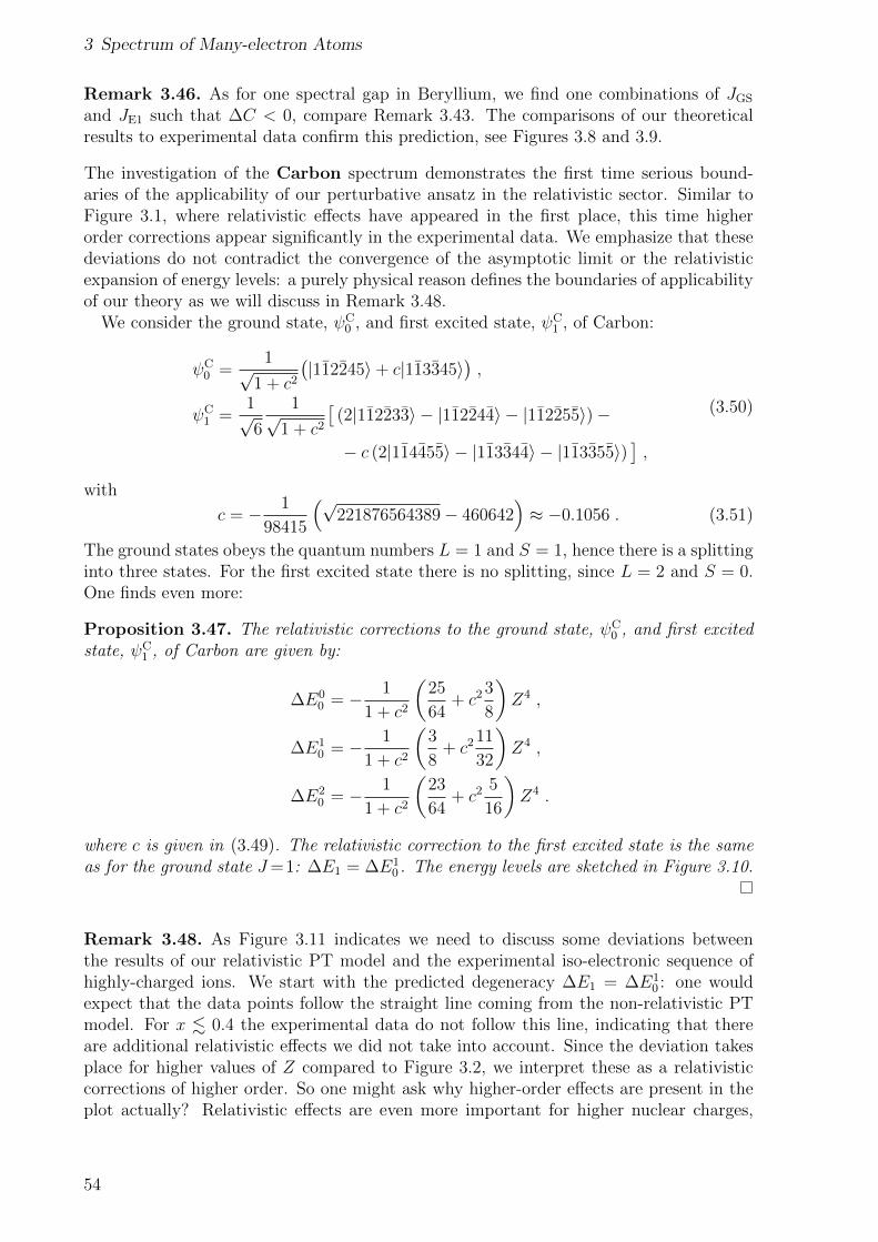
3 Spectrum of Many-electron Atoms
Remark 3.46. As for one spectral gap in Beryllium, we find one combinations of JGS
and JE1 such that ∆C < 0, compare Remark 3.43. The comparisons of our theoreticalresults to experimental data confirm this prediction, see Figures 3.8 and 3.9.
The investigation of the Carbon spectrum demonstrates the first time serious bound-aries of the applicability of our perturbative ansatz in the relativistic sector. Similar toFigure 3.1, where relativistic effects have appeared in the first place, this time higherorder corrections appear significantly in the experimental data. We emphasize that thesedeviations do not contradict the convergence of the asymptotic limit or the relativisticexpansion of energy levels: a purely physical reason defines the boundaries of applicabilityof our theory as we will discuss in Remark 3.48.
We consider the ground state, ψC0 , and first excited state, ψC
1 , of Carbon:
ψC0 =
1√1 + c2
(|112245〉+ c|113345〉
),
ψC1 =
1√6
1√1 + c2
[(2|112233〉 − |112244〉 − |112255〉)−
− c (2|114455〉 − |113344〉 − |113355〉)],
(3.50)
with
c = − 1
98415
(√221876564389− 460642
)≈ −0.1056 . (3.51)
The ground states obeys the quantum numbers L = 1 and S = 1, hence there is a splittinginto three states. For the first excited state there is no splitting, since L = 2 and S = 0.One finds even more:
Proposition 3.47. The relativistic corrections to the ground state, ψC0 , and first excited
state, ψC1 , of Carbon are given by:
∆E00 = − 1
1 + c2
(25
64+ c2 3
8
)Z4 ,
∆E10 = − 1
1 + c2
(3
8+ c2 11
32
)Z4 ,
∆E20 = − 1
1 + c2
(23
64+ c2 5
16
)Z4 .
where c is given in (3.49). The relativistic correction to the first excited state is the sameas for the ground state J=1: ∆E1 = ∆E1
0 . The energy levels are sketched in Figure 3.10.
Remark 3.48. As Figure 3.11 indicates we need to discuss some deviations betweenthe results of our relativistic PT model and the experimental iso-electronic sequence ofhighly-charged ions. We start with the predicted degeneracy ∆E1 = ∆E1
0 : one wouldexpect that the data points follow the straight line coming from the non-relativistic PTmodel. For x . 0.4 the experimental data do not follow this line, indicating that thereare additional relativistic effects we did not take into account. Since the deviation takesplace for higher values of Z compared to Figure 3.2, we interpret these as a relativisticcorrections of higher order. So one might ask why higher-order effects are present in theplot actually? Relativistic effects are even more important for higher nuclear charges,
54
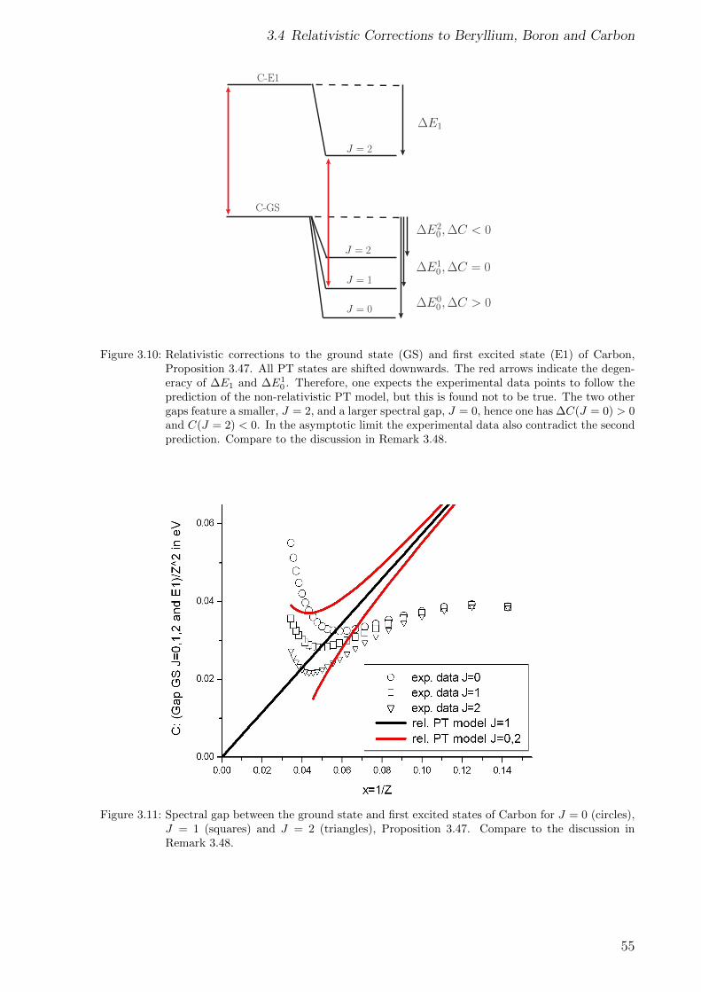
3.4 Relativistic Corrections to Beryllium, Boron and Carbon
C-E1
C-GS
J = 2
J = 1
ΔE20 ,ΔC < 0
ΔE1
ΔE10 ,ΔC = 0
J = 2
J = 0ΔE0
0 ,ΔC > 0
Figure 3.10: Relativistic corrections to the ground state (GS) and first excited state (E1) of Carbon,Proposition 3.47. All PT states are shifted downwards. The red arrows indicate the degen-eracy of ∆E1 and ∆E1
0 . Therefore, one expects the experimental data points to follow theprediction of the non-relativistic PT model, but this is found not to be true. The two othergaps feature a smaller, J = 2, and a larger spectral gap, J = 0, hence one has ∆C(J = 0) > 0and C(J = 2) < 0. In the asymptotic limit the experimental data also contradict the secondprediction. Compare to the discussion in Remark 3.48.
Figure 3.11: Spectral gap between the ground state and first excited states of Carbon for J = 0 (circles),J = 1 (squares) and J = 2 (triangles), Proposition 3.47. Compare to the discussion inRemark 3.48.
55
3 Spectrum of Many-electron Atoms
hence in the asymptotic limit our first-order ansatz in the relativistic sector runs outof physical applicability. The perturbative ansatz in large nuclear charges and a largespeed of light is fine from a mathematical point of view. Physically, we need to take thefull relativistic theory into account when combining both expansions. However, there isalways just a finite number of experimental data points available and the magnitude ofthe higher-order corrections for different chemical elements differ strongly, hence there isindeed a satisfactory agreement between our theory and experimental data as shown forLithium, Beryllium, and Boron.
We emphasize that the qualitative agreement for not too high Z does still hold in thecarbon case: for J = 0 we expect a positive, for J = 2 we expect a negative relativisticcorrection. ∆C(J = 0) > 0 is confirmed by Figure 3.11, if thought not quantitatively.Also ∆C(J = 2) < 0 is confirmed when restricting to the region of applicability of thefirst-order ansatz: 0.04 . x . 0.10. In comparison to the experimental data for J = 1their downward deviation holds. Due to the strong Z-dependence, higher-order correctionsbecome more important for x . 0.04.
56
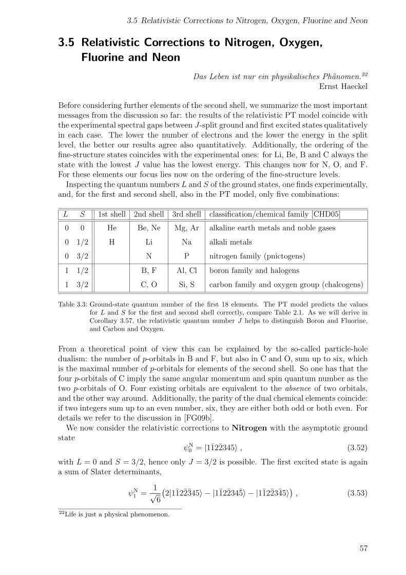
3.5 Relativistic Corrections to Nitrogen, Oxygen, Fluorine and Neon
3.5 Relativistic Corrections to Nitrogen, Oxygen,Fluorine and Neon
Das Leben ist nur ein physikalisches Phanomen.22
Ernst Haeckel
Before considering further elements of the second shell, we summarize the most importantmessages from the discussion so far: the results of the relativistic PT model coincide withthe experimental spectral gaps between J-split ground and first excited states qualitativelyin each case. The lower the number of electrons and the lower the energy in the splitlevel, the better our results agree also quantitatively. Additionally, the ordering of thefine-structure states coincides with the experimental ones: for Li, Be, B and C always thestate with the lowest J value has the lowest energy. This changes now for N, O, and F.For these elements our focus lies now on the ordering of the fine-structure levels.
Inspecting the quantum numbers L and S of the ground states, one finds experimentally,and, for the first and second shell, also in the PT model, only five combinations:
L S 1st shell 2nd shell 3rd shell classification/chemical family [CHD05]
0 0 He Be, Ne Mg, Ar alkaline earth metals and noble gases
0 1/2 H Li Na alkali metals
0 3/2 N P nitrogen family (pnictogens)
1 1/2 B, F Al, Cl boron family and halogens
1 3/2 C, O Si, S carbon family and oxygen group (chalcogens)
Table 3.3: Ground-state quantum number of the first 18 elements. The PT model predicts the valuesfor L and S for the first and second shell correctly, compare Table 2.1. As we will derive inCorollary 3.57, the relativistic quantum number J helps to distinguish Boron and Fluorine,and Carbon and Oxygen.
From a theoretical point of view this can be explained by the so-called particle-holedualism: the number of p-orbitals in B and F, but also in C and O, sum up to six, whichis the maximal number of p-orbitals for elements of the second shell. So one has that thefour p-orbitals of C imply the same angular momentum and spin quantum number as thetwo p-orbitals of O. Four existing orbitals are equivalent to the absence of two orbitals,and the other way around. Additionally, the parity of the dual chemical elements coincide:if two integers sum up to an even number, six, they are either both odd or both even. Fordetails we refer to the discussion in [FG09b].
We now consider the relativistic corrections to Nitrogen with the asymptotic groundstate
ψN0 = |1122345〉 , (3.52)
with L = 0 and S = 3/2, hence only J = 3/2 is possible. The first excited state is againa sum of Slater determinants,
ψN1 =
1√6
(2|1122345〉 − |1122345〉 − |1122345〉
), (3.53)
22Life is just a physical phenomenon.
57
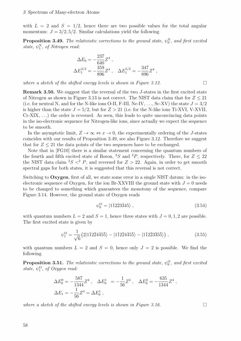
3 Spectrum of Many-electron Atoms
with L = 2 and S = 1/2, hence there are two possible values for the total angularmomentum: J = 3/2, 5/2. Similar calculations yield the following
Proposition 3.49. The relativistic corrections to the ground state, ψN0 , and first excited
state, ψN1 , of Nitrogen read:
∆E0 = −237
640Z4 ,
∆E3/21 = −359
896Z4 , ∆E
5/21 = −347
896Z4 ,
where a sketch of the shifted energy levels is shown in Figure 3.12.
Remark 3.50. We suggest that the reversal of the two J-states in the first excited stateof Nitrogen as shown in Figure 3.13 is not correct. The NIST data claim that for Z ≤ 21(i.e. for neutral N, and for the N-like ions O-II, F-III, Ne-IV, . . ., Sc-XV) the state J = 3/2is higher than the state J = 5/2, but for Z > 21 (i.e. for the N-like ions Ti-XVI, V-XVII,Cr-XIX, . . .) the order is reversed. As seen, this leads to quite unconvincing data pointsin the iso-electronic sequence for Nitrogen-like ions, since actually we expect the sequenceto be smooth.
In the asymptotic limit, Z →∞⇔ x→ 0, the experimentally ordering of the J-statescoincides with our results of Proposition 3.49, see also Figure 3.12. Therefore we suggestthat for Z ≤ 21 the data points of the two sequences have to be exchanged.
Note that in [FG10] there is a similar statement concerning the quantum numbers ofthe fourth and fifth excited state of Boron, 2S and 2P , respectively. There, for Z ≤ 22the NIST data claim 2S <2 P , and reversed for Z > 22. Again, in order to get smoothspectral gaps for both states, it is suggested that this reversal is not correct.
Switching to Oxygen, first of all, we state some error in a single NIST datum: in the iso-electronic sequence of Oxygen, for the ion Br-XXVIII the ground state with J = 0 needsto be changed to something which guarantees the monotony of the sequence, compareFigure 3.14. However, the ground state of Oxygen reads
ψO0 = |11223345〉 , (3.54)
with quantum numbers L = 2 and S = 1, hence three states with J = 0, 1, 2 are possible.The first excited state is given by
ψO1 =
1√6
(2|11224455〉 − |11224455〉 − |11223355〉
), (3.55)
with quantum numbers L = 2 and S = 0, hence only J = 2 is possible. We find thefollowing
Proposition 3.51. The relativistic corrections to the ground state, ψO0 , and first excited
state, ψO1 , of Oxygen read:
∆E00 = − 587
1344Z4 , ∆E1
0 = − 1
56Z4 , ∆E2
0 = − 635
1344Z4 ,
∆E1 = − 1
56Z4 = ∆E1
0 ,
where a sketch of the shifted energy levels is shown in Figure 3.16.
58
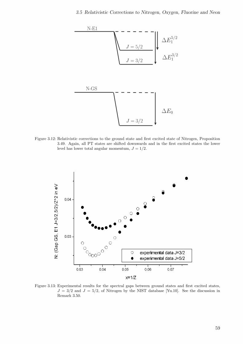
3.5 Relativistic Corrections to Nitrogen, Oxygen, Fluorine and Neon
N-E1
N-GS
J = 5/2
J = 3/2
J = 3/2
ΔE5/21
ΔE3/21
ΔE0
Figure 3.12: Relativistic corrections to the ground state and first excited state of Nitrogen, Proposition3.49. Again, all PT states are shifted downwards and in the first excited states the lowerlevel has lower total angular momentum, J = 1/2.
Figure 3.13: Experimental results for the spectral gaps between ground states and first excited states,J = 3/2 and J = 5/2, of Nitrogen by the NIST database [Yu.10]. See the discussion inRemark 3.50.
59
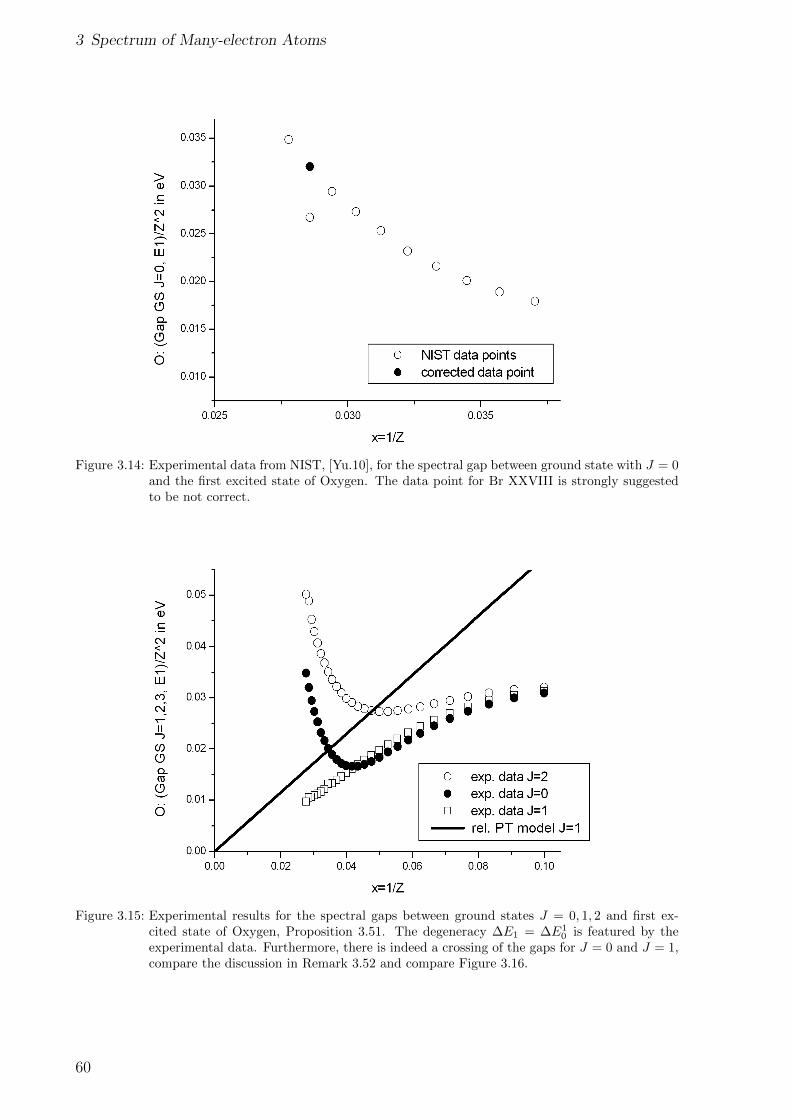
3 Spectrum of Many-electron Atoms
Figure 3.14: Experimental data from NIST, [Yu.10], for the spectral gap between ground state with J = 0and the first excited state of Oxygen. The data point for Br XXVIII is strongly suggestedto be not correct.
Figure 3.15: Experimental results for the spectral gaps between ground states J = 0, 1, 2 and first ex-cited state of Oxygen, Proposition 3.51. The degeneracy ∆E1 = ∆E1
0 is featured by theexperimental data. Furthermore, there is indeed a crossing of the gaps for J = 0 and J = 1,compare the discussion in Remark 3.52 and compare Figure 3.16.
60
3.5 Relativistic Corrections to Nitrogen, Oxygen, Fluorine and Neon
O-E1
O-GS
J = 2
J = 0
ΔE1
ΔE20
J = 1ΔE1
0
J = 2
ΔE00
Figure 3.16: Relativistic corrections to the ground state and first excited state of Oxygen, Proposition3.51. The lowest level of the split ground state has J = 2, which is confirmed by theexperimental data. The ordering E(J = 0) < E(J = 1) holds experimentally only in theasymptotic limit, see the reversal in Figure 3.15. For the ground state of neutral Oxygen onefinds experimentally the reversed ordering. The red arrows indicate again the degeneracy∆E1 = ∆E1
0 , also found in the experimental data.
Remark 3.52. For Oxygen we expect from Proposition 3.51 that the ground state fea-tures a splitting into three energy levels with the ordering E(J=2) < E(J=0) < E(J=1).This ordering is different to the cases we had before since the values of J do not just followthe pattern “high to low” or “low to high”, but they are really mixed. The ground state ofneutral Oxygen, J = 2, is confirmed experimentally, but the predicted ordering for J = 0and J = 1 is not found experimentally, but one finds: E(J = 2) < E(J = 1) < E(J = 0).However, the iso-electronic sequence for Oxygen features an interesting crossing of theenergy levels for J = 1 and J = 0. In contrast to Nitrogen, compare Remark 3.50, thisreversal happens smoothly, so we consider the experimental data to be correct. Therefore,the theoretically predicted ordering appears to be correct for large values of the nuclearcharge. This is consistent with our perturbative approach and the convergence in theasymptotic limit Z → ∞. Note that for all data points the spectral gap between J = 2and the first excited state is the largest one, hence this is also the ground state of neutralOxygen, in agreement with our results.
Furthermore, the predicted degeneracy ∆E1 = ∆E10 is found in the experimental spectral
gaps for Oxygen: the accordant data points (squares in Figure 3.15) seem to follow thestraight line from the, even non-relativistic, PT model. Additionally, for the other statesJ = 2 and J = 1 we expect, besides their ordering, a positive relativistic corrections,which is also featured by the experimental data:
∆C(J = 2) =611
1344, and ∆C(J = 0) =
563
1344. (3.56)
61
3 Spectrum of Many-electron Atoms
Now we start the investigation of Fluorine. Its ground state reads
ψF0 = |112234455〉 , (3.57)
with L = 1 and S = 1/2, hence two states, J = 1/2, 3/2 are possible. The first excitedstate is quite similar,
ψF1 = |112334455〉 , (3.58)
with L = 0 and S = 1/2, hence only J = 1/2 is possible. Again, we skip the explicitcalculation and state the following
Proposition 3.53. The relativistic corrections to the ground state, ψF0 , and first excited
state, ψF1 , of Fluorine read:
∆E1/20 = −409
896Z4 , ∆E
3/20 = −449
896Z4 ,
∆E1 = −397
896Z4 ,
where a sketch of the shifted energy levels is shown in Figure 3.17.
Remark 3.54. In Fluorine we do not expect any degeneracy but the relativistic correctionfor the spectral gap between ground state J = 1/2 and first excited state is much smallerthan for J = 3/2 in the ground state:
∆C(J = 1/2) =3
224≈ 0.01 , and ∆C(J = 3/2) =
13
224≈ 0.06 . (3.59)
This qualitative behavior can be observed in the experimental data, but the positiverelativistic correction is not yet visible for the experimentally available ions in the iso-electronic sequence for Fluorine.
In Figure 3.18 we show again also the quantitative agreement between our theoreticalresults and the experimental data. As already concluded at the beginning of this sectionthe lower the energy state the better the qualitative agreement. This statement does holdalso for chemical elements with more than six electrons.
The last chemical element we consider in this thesis is Neon. The PT model offers onlythe ground state,
ψNe0 = |1122334455〉 , (3.60)
with L = 0 and S = 0, hence no splitting of the ground state takes place: only J = 0 ispossible. We find the following
Proposition 3.55. The relativistic correction to the ground state of Neon reads:
∆E0 = −15
32Z4 .
Remark 3.56. Since in Neon all ten available hydrogen orbitals, |i〉, |i〉 for i = 1, . . . , 5,are occupied, excited states can not be derived in the PT model.
62
3.5 Relativistic Corrections to Nitrogen, Oxygen, Fluorine and Neon
F-E1
F-GS
J = 1/2
J = 1/2
J = 3/2
ΔE1/20
ΔE1
ΔE3/20
Figure 3.17: Relativistic corrections to the ground state and first excited state of Fluorine, Proposition3.53. The lowest level of the split ground state has J = 3/2, which is confirmed by theexperimental data.
Figure 3.18: Experimental results for the spectral gaps between ground states J = 1/2, 3/2 and firstexcited state of Fluorine, Proposition 3.53. The small predicted relativistic correction forJ = 1/2 is featured by the experimental data, actually it seems to follow the non-relativisticprediction.
63
3 Spectrum of Many-electron Atoms
As claimed at the beginning of this section we now conclude our findings in Corollary3.57: the chemical elements of the second shell whose ground states feature the angular-momentum quantum number L = 1 are distinguishable when taking the relativistic quan-tum number J into account:
Corollary 3.57. For the two pairs of quantum numbers (L, S) = (1, 1/2) and (L, S) =(1, 3/2) there is a splitting into two distinguishable energy levels with J = 1/2, 3/2 andJ = 3/2, 5/2, respectively.
(a) The ground state of Boron has the quantum number (L, S, J) = (1, 1/2, 1/2). Itsdual, Fluorine, features (L, S, J) = (1, 1/2, 3/2).
(b) The ground state of Carbon has the quantum number (L, S, J) = (1, 3/2, 1/2). Itsdual, Oxygen, features (L, S, J) = (1, 3/2, 5/2).
In the relativistic setup only ground states of two second-shell elements, Beryllium andNeon, remain indistinguishable in the quantum numbers (L, S, J) = (0, 0, 0).
Proof. For Boron and Fluorine one only has to inspect Propositions 3.44 and 3.53. ForCarbon and Oxygen the relevant Propositions are 3.47 and 3.51.
Remark 3.58. The experimental data confirm our theoretical results: for Oxygen andFluorine the ground states feature the highest possible value for J , whereas for Boron andCarbon the lowest possible J is realized in nature.
64
3.6 Non-local Relativistic Corrections
3.6 Non-local Relativistic Corrections
Wer einen Fehler gemacht hat und ihn nicht korrigiert, begeht einen zweiten.23
Konfuzius
So far we have derived the relativistic corrections in the local model, compare section 3.2.2.The fact that the asymptotic states we are dealing with coincide with the Schrodingerstates in the limit Z →∞ has motivated us to restrict to the diagonal terms of L · S.
The set of good quantum numbers in the non-relativistic setup is given by (L, S, L3, S3),where we can choose without loss of generality one component of L and S. This is alsohow the wave functions of the ground state from Table 3.1 are chosen: L3 = 0 andS3 = L+ S is maximal. As already done in the proof of Lemma 3.25 for the one-particlestate, we now switch to bases of the ground state where the many-particle operators L2,S2, J2 and J3 are diagonal. Again, without loss of generality, we choose for a giveneigenvalue J the corresponding magnetic quantum number to be maximal: J3 = J . Thetransformation between these two bases is known as Clebsch-Gordan decomposition,and we denote the new states by |L, S, J, J3〉, or, if the corresponding chemical element isclear, by |J, J3〉. Having an orthogonal basis in the non-relativistic setup, the new basisis again orthogonal. A general discussion of this technique can be found, for instance, in[FH91]. We only note that the dimensions of the ground-state in the classical and therelativistic basis indeed coincide, since the degeneracy for a given J is 2J + 1:
L+S∑J=|L−S|
(2J + 1) = (1 + L+ S − |L− S|)(1 + L+ S + |L− S|) =
= 1 + 2(L+ S) + 2LS − |L− S|2 = (2L+ 1)(2S + 1) .
(3.61)
In Table 3.4 we state the Clebsch-Gordan decomposition for all ground and first excitedstates. Table 3.5 summarizes the degeneracies of the ground-state and first-excited-stateeigenspaces of the non-relativistic PT model. For the non-interacting ground state wehave, [FG09b]:
dimV0(N) =
(2
N
), for N = 1, 2, dimV0(N) =
(8
N − 2
), for 3 ≤ N ≤ 10 .
(3.62)As already discussed, the dimensions of the interacting ground and first excited statesdepend on their symmetry, described by the eigenvalues L and S:
dim(·)(N) = (2L+ 1)(2S + 1) .
In the following we will discuss in detail the case of the first excited state of Lithium andBeryllium in order to illustrate the similarities and differences to the local model. Westart with Lithium: the interacting first excited state is six-dimensional, spanned by theorthogonal bases of non-relativistic eigenfunctions
E1(3) = span|11i〉, |11i〉 : i = 3, 4, 5 . (3.63)
23If you make a mistake and do not correct it, this is called a mistake.
65
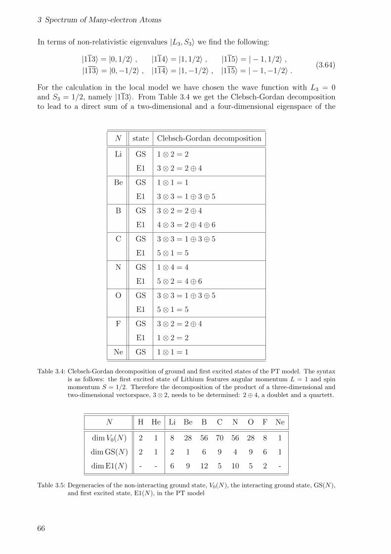
3 Spectrum of Many-electron Atoms
In terms of non-relativistic eigenvalues |L3, S3〉 we find the following:
|113〉 = |0, 1/2〉 , |114〉 = |1, 1/2〉 , |115〉 = | − 1, 1/2〉 ,|113〉 = |0,−1/2〉 , |114〉 = |1,−1/2〉 , |115〉 = | − 1,−1/2〉 . (3.64)
For the calculation in the local model we have chosen the wave function with L3 = 0and S3 = 1/2, namely |113〉. From Table 3.4 we get the Clebsch-Gordan decompositionto lead to a direct sum of a two-dimensional and a four-dimensional eigenspace of the
N state Clebsch-Gordan decomposition
Li GS 1⊗ 2 = 2
E1 3⊗ 2 = 2⊕ 4
Be GS 1⊗ 1 = 1
E1 3⊗ 3 = 1⊕ 3⊕ 5
B GS 3⊗ 2 = 2⊕ 4
E1 4⊗ 3 = 2⊕ 4⊕ 6
C GS 3⊗ 3 = 1⊕ 3⊕ 5
E1 5⊗ 1 = 5
N GS 1⊗ 4 = 4
E1 5⊗ 2 = 4⊕ 6
O GS 3⊗ 3 = 1⊕ 3⊕ 5
E1 5⊗ 1 = 5
F GS 3⊗ 2 = 2⊕ 4
E1 1⊗ 2 = 2
Ne GS 1⊗ 1 = 1
Table 3.4: Clebsch-Gordan decomposition of ground and first excited states of the PT model. The syntaxis as follows: the first excited state of Lithium features angular momentum L = 1 and spinmomentum S = 1/2. Therefore the decomposition of the product of a three-dimensional andtwo-dimensional vectorspace, 3⊗ 2, needs to be determined: 2⊕ 4, a doublet and a quartett.
N H He Li Be B C N O F Ne
dimV0(N) 2 1 8 28 56 70 56 28 8 1
dim GS(N) 2 1 2 1 6 9 4 9 6 1
dim E1(N) - - 6 9 12 5 10 5 2 -
Table 3.5: Degeneracies of the non-interacting ground state, V0(N), the interacting ground state, GS(N),and first excited state, E1(N), in the PT model
66
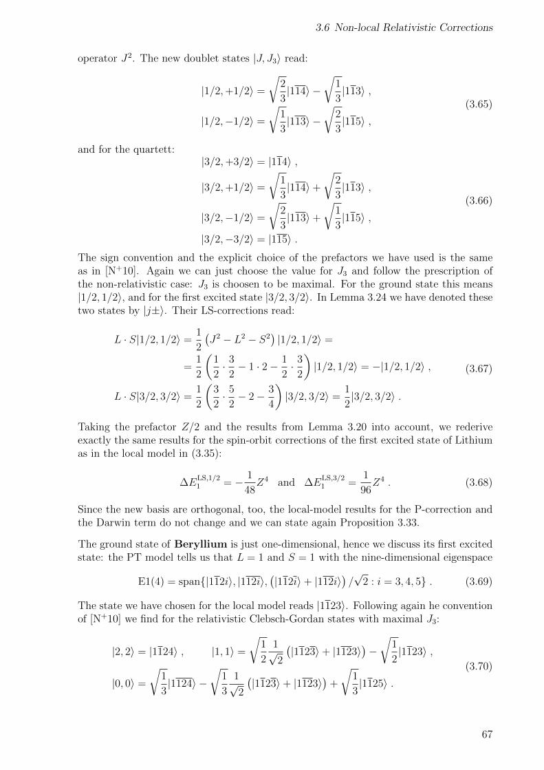
3.6 Non-local Relativistic Corrections
operator J2. The new doublet states |J, J3〉 read:
|1/2,+1/2〉 =
√2
3|114〉 −
√1
3|113〉 ,
|1/2,−1/2〉 =
√1
3|113〉 −
√2
3|115〉 ,
(3.65)
and for the quartett:|3/2,+3/2〉 = |114〉 ,
|3/2,+1/2〉 =
√1
3|114〉+
√2
3|113〉 ,
|3/2,−1/2〉 =
√2
3|113〉+
√1
3|115〉 ,
|3/2,−3/2〉 = |115〉 .
(3.66)
The sign convention and the explicit choice of the prefactors we have used is the sameas in [N+10]. Again we can just choose the value for J3 and follow the prescription ofthe non-relativistic case: J3 is choosen to be maximal. For the ground state this means|1/2, 1/2〉, and for the first excited state |3/2, 3/2〉. In Lemma 3.24 we have denoted thesetwo states by |j±〉. Their LS-corrections read:
L · S|1/2, 1/2〉 =1
2
(J2 − L2 − S2
)|1/2, 1/2〉 =
=1
2
(1
2· 3
2− 1 · 2− 1
2· 3
2
)|1/2, 1/2〉 = −|1/2, 1/2〉 ,
L · S|3/2, 3/2〉 =1
2
(3
2· 5
2− 2− 3
4
)|3/2, 3/2〉 =
1
2|3/2, 3/2〉 .
(3.67)
Taking the prefactor Z/2 and the results from Lemma 3.20 into account, we rederiveexactly the same results for the spin-orbit corrections of the first excited state of Lithiumas in the local model in (3.35):
∆ELS,1/21 = − 1
48Z4 and ∆E
LS,3/21 =
1
96Z4 . (3.68)
Since the new basis are orthogonal, too, the local-model results for the P-correction andthe Darwin term do not change and we can state again Proposition 3.33.
The ground state of Beryllium is just one-dimensional, hence we discuss its first excitedstate: the PT model tells us that L = 1 and S = 1 with the nine-dimensional eigenspace
E1(4) = span|112i〉, |112i〉,(|112i〉+ |112i〉
)/√
2 : i = 3, 4, 5 . (3.69)
The state we have chosen for the local model reads |1123〉. Following again he conventionof [N+10] we find for the relativistic Clebsch-Gordan states with maximal J3:
|2, 2〉 = |1124〉 , |1, 1〉 =
√1
2
1√2
(|1123〉+ |1123〉
)−√
1
2|1123〉 ,
|0, 0〉 =
√1
3|1124〉 −
√1
3
1√2
(|1123〉+ |1123〉
)+
√1
3|1125〉 .
(3.70)
67
3 Spectrum of Many-electron Atoms
From this we find for the eigenvalues of L · S:
L · S|2, 2〉 = |2, 2〉 , L · S|1, 1〉 = −|1, 1〉 , L · S|0, 0〉 = −2|0, 0〉 . (3.71)
Since the P-contribution and Darwin term can be again recycled from our discussion inthe local model, we arrive at the following
Proposition 3.59. In the non-local PT model the relativistic corrections to the groundand first excited state of Beryllium are given by:
∆E0 = − 1
1 + c2
(21
64+ c2 55
192
)Z4 ,
∆E01 = − 67
192Z4 , ∆E1
1 = − 63
192Z4 , ∆E2
1 = − 55
192Z4 ,
where c is given in (3.42).
Remark 3.60. The comparison of the last results in Proposition 3.59 to their localversions in Proposition 3.42 yields deviations of only a few percent: in the ground stateonly the coefficient of c2/(1 + c2) differs: −55/192 + 19/64 ≈ 1.0%.
In the first excited state the deviation for J = 0 reads (−67 + 63)/192 ≈ −2.1%. ForJ = 1 one finds (−63 + 60)/192 ≈ −1.6%, and for J = 2 one has (−55 + 57)/192 ≈ 1.0%.
Note that the deviations for J = 0, 1 lead to a further downwards shift of the finestructure states, whereas for J = 2 the predicted state of the local model is shiftedslightly upwars. However, the deviations are not very large and Figures 3.6 and 3.7still hold, particularly the discussion in Remark 3.43: for instance the new value for therelativistically-corrected energy gap
∆C(J = 0) = − c2
1 + c2
1
16≈ −0.0031 · 10−3 < 0 ,
which is twice the value in the local model (3.47). The qualitative feature that thiscorrection is negative does still hold in the non-local model.
We can also derive the corrections for Boron: again, the P-contribution and the Darwinterm can be used from our discussion of the local model.
Proposition 3.61. In the non-local PT model the relativistic corrections to the groundand first excited state of Boron are given by:
∆E1/20 = − 1
1 + c2
(47
128+ c2 125
384
)Z4 , ∆E
3/20 = − 1
1 + c2
(43
128+ c2 113
384
)Z4 ,
∆E1/21 = −145
384Z4 , ∆E
3/21 − 133
384Z4 , ∆E
5/21 = −113
384Z4 ,
where c is given in (3.49).
Remark 3.62. Again, the deviations between the results in Proposition 3.61 and theirlocal version in Proposition 3.44 are small. The largest deviations occurs for ∆E
1/21 :
(−145 + 133)/384 ≈ 3.1%.
Remark 3.63. As discussed in section 3.5, the experimental ground state of chemicalelements with 7 ≤ N ≤ 10 feature the highest possible value for J to be the lowest fine
68
3.6 Non-local Relativistic Corrections
structure state. In particular, two pairs of elements, namely Boron and Fluorine, andCarbon and Oxygen, have the same ground state symmetry on the non-relativistic level,but the total angular momentum was found experimentally to distinguish the membersof each pair. In the local PT model we have used the parameter N− to describe theelectronic structure. This parameter has made it possible to describe this behavior.
Now, as Table 3.4 shows, for a given angular momentum and spin momentum, theClebsch-Gordan decomposition does not know about the number of electrons. Therefore,the decompositions for Boron and Fluorine lead to the same |J, J3〉 states, hence also tothe same eigenvalues of the operator L · S. In the end the split state with the lowestpossible value for J appears to be the ground state.
We interpret this as follows: the asymptotic vector spaces for the ground states arederived using a perturbative ansatz in the Coulomb interaction between the electrons. Inthe limit Z →∞ the electron-nucleus interaction is the dominant interaction. As alreadystates in Remark 3.32, this limit is actually incompatible with perturbation theory in therelativistic sector. However, we use the operator L · S, with some additional prefactor,which occurs in the non-relativistic limit of Dirac theory for non-degenerate eigenvalues.From experiments it is known that for heavy nuclei, i.e. for atoms or ions which carry alarge nuclear charge Z, the so-called JJ-coupling instead of the LS-coupling is apparent.The physical condition for the LS-coupling is given by large effects of electromagneticinteraction between different electrons, but small effects of the spin-orbit coupling. Sincethe latter ones are proportional to Z4, whereas the electron-electron interaction are pro-portional to Z, compare (3.30), we actually have to implement the JJ-coupling in ourmodel.
69

4 Summary and Conclusion
Questo grandissimo libro [...] – io dico l’universo – [...] e scritto in lingua matematica.1
Galileo Galilei
We state from [FG09b] all asymptotic PT eigenfunctions for the ground states and firstexcited states we have used for our calculations. We also summarize all energy levels andtheir relativistic corrections we have derived in this thesis whithin the local model: Tables4.1, 4.2 and 4.3. A summary which emphasizes the spin structure, described by N±, andthe theoretical J-ordering of the energy levels is shown in Table 4.4.
We have seen that doing perturbation theory in the relativistic sector on the asymptoticPT states asks for a careful treatment of the two limits, since, for a fixed finite value ofthe speed of light, the relativistic effects become dominant for large values of the nuclearcharge. One might treat the two limits, Z → ∞ and c0 → ∞, in such a way that thehierarchy Z c0 is still respected.
The second conceptual question is due to the form of the spin-orbit coupling for N -electron systems. The one-particle LS term emerges in the non-relativistic limit of Diractheory in a rigorous way. However, there is no N -particle Dirac theory; one actuallyhas to implement concepts of quantum fields. In particular, the spatial part of the LSterm, |x|−3, cannot be generalized ad hoc to N -electron systems. In this thesis we haveused a local model which restricts the LS term to the diagonal contributions. Due to theasymptotic states we are dealing with, this seems to be a resonable treatment: we treatboth electric and magnetic interactions between different electrons to be small comparedto the interaction between one electron and the higly charged nucleus. However, therelativistic setup suggests in the first place to have only electromagnetic interactions inmind and not to distinguish between electric and magnetic ones. The local model takesthis aspect consistently into account.
Describing the spin structure by N±, we have been able to model the experimentalfact that for Oxygen and Fluorine the highest possible value for J appears to be theground state, whereas for their dual elements, Carbon and Boron, respectively, the lowestpossible value of J imply the lowest energy. In the semi-empirical Hund’s rules this reveralis described by inserting a minus sign in front of the LS term for elements N = 7, 8, 9, 10.
In conclusion, the local model implements in a consistent way relativistic effects intothe non-relativistic PT model. The treatment of the concurrent limits, Z → ∞ andc0 → ∞, needs to guarantee the applicability of first-order perturbation theory in therelativistic sector. In comparison to experimental data from the NIST database we findgood qualitative agreements for the Z2-scaled spectral gaps. In particular, the predictionof relativistic degeneracies in Lithium or Oxygen are featured by nature.
1This grand book [...] – I mean the universe – [...] is written in the language of mathematics.
71
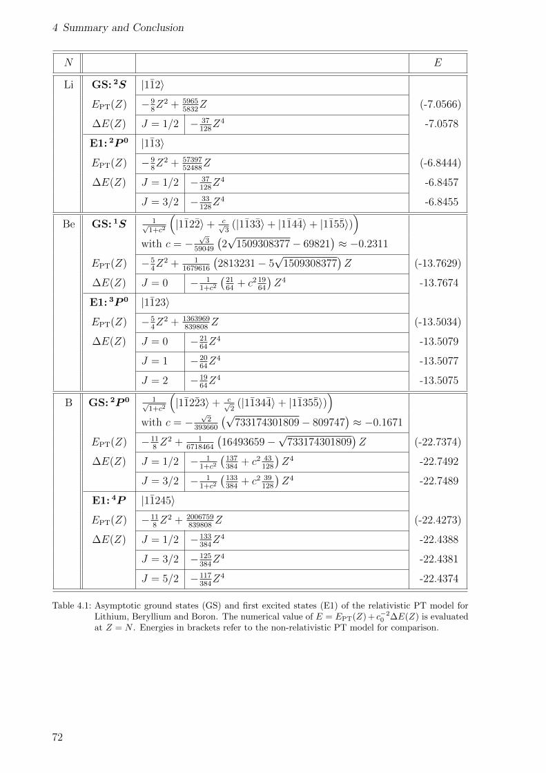
4 Summary and Conclusion
N E
Li GS: 2S |112〉EPT(Z) −9
8Z2 + 5965
5832Z (-7.0566)
∆E(Z) J = 1/2 − 37128Z4 -7.0578
E1: 2P 0 |113〉EPT(Z) −9
8Z2 + 57397
52488Z (-6.8444)
∆E(Z) J = 1/2 − 37128Z4 -6.8457
J = 3/2 − 33128Z4 -6.8455
Be GS: 1S 1√1+c2
(|1122〉+ c√
3(|1133〉+ |1144〉+ |1155〉)
)with c = −
√3
59049
(2√
1509308377− 69821)≈ −0.2311
EPT(Z) −54Z2 + 1
1679616
(2813231− 5
√1509308377
)Z (-13.7629)
∆E(Z) J = 0 − 11+c2
(2164
+ c2 1964
)Z4 -13.7674
E1: 3P 0 |1123〉EPT(Z) −5
4Z2 + 1363969
839808Z (-13.5034)
∆E(Z) J = 0 −2164Z4 -13.5079
J = 1 −2064Z4 -13.5077
J = 2 −1964Z4 -13.5075
B GS: 2P 0 1√1+c2
(|11223〉+ c√
2(|11344〉+ |11355〉)
)with c = −
√2
393660
(√733174301809− 809747
)≈ −0.1671
EPT(Z) −118Z2 + 1
6718464
(16493659−
√733174301809
)Z (-22.7374)
∆E(Z) J = 1/2 − 11+c2
(137384
+ c2 43128
)Z4 -22.7492
J = 3/2 − 11+c2
(133384
+ c2 39128
)Z4 -22.7489
E1: 4P |11245〉EPT(Z) −11
8Z2 + 2006759
839808Z (-22.4273)
∆E(Z) J = 1/2 −133384Z4 -22.4388
J = 3/2 −125384Z4 -22.4381
J = 5/2 −117384Z4 -22.4374
Table 4.1: Asymptotic ground states (GS) and first excited states (E1) of the relativistic PT model forLithium, Beryllium and Boron. The numerical value of E = EPT(Z) + c−2
0 ∆E(Z) is evaluatedat Z = N . Energies in brackets refer to the non-relativistic PT model for comparison.
72
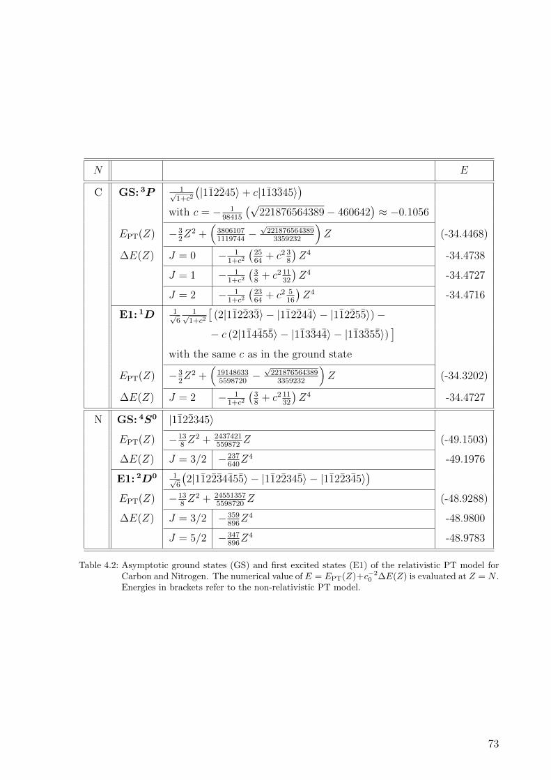
N E
C GS: 3P 1√1+c2
(|112245〉+ c|113345〉
)with c = − 1
98415
(√221876564389− 460642
)≈ −0.1056
EPT(Z) −32Z2 +
(38061071119744
−√
2218765643893359232
)Z (-34.4468)
∆E(Z) J = 0 − 11+c2
(2564
+ c2 38
)Z4 -34.4738
J = 1 − 11+c2
(38
+ c2 1132
)Z4 -34.4727
J = 2 − 11+c2
(2364
+ c2 516
)Z4 -34.4716
E1: 1D 1√6
1√1+c2
[(2|112233〉 − |112244〉 − |112255〉)−− c (2|114455〉 − |113344〉 − |113355〉)
]with the same c as in the ground state
EPT(Z) −32Z2 +
(191486335598720
−√
2218765643893359232
)Z (-34.3202)
∆E(Z) J = 2 − 11+c2
(38
+ c2 1132
)Z4 -34.4727
N GS: 4S0 |1122345〉EPT(Z) −13
8Z2 + 2437421
559872Z (-49.1503)
∆E(Z) J = 3/2 −237640Z4 -49.1976
E1: 2D0 1√6
(2|112234455〉 − |1122345〉 − |1122345〉
)EPT(Z) −13
8Z2 + 24551357
5598720Z (-48.9288)
∆E(Z) J = 3/2 −359896Z4 -48.9800
J = 5/2 −347896Z4 -48.9783
Table 4.2: Asymptotic ground states (GS) and first excited states (E1) of the relativistic PT model forCarbon and Nitrogen. The numerical value of E = EPT(Z)+c−2
0 ∆E(Z) is evaluated at Z = N .Energies in brackets refer to the non-relativistic PT model.
73
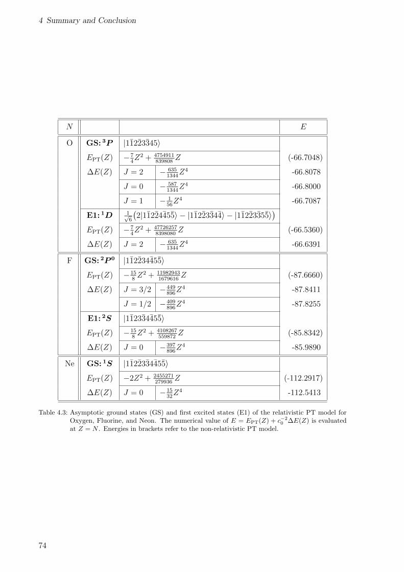
4 Summary and Conclusion
N E
O GS: 3P |11223345〉EPT(Z) −7
4Z2 + 4754911
839808Z (-66.7048)
∆E(Z) J = 2 − 6351344
Z4 -66.8078
J = 0 − 5871344
Z4 -66.8000
J = 1 − 156Z4 -66.7087
E1: 1D 1√6
(2|11224455〉 − |11223344〉 − |11223355〉
)EPT(Z) −7
4Z2 + 47726257
8398080Z (-66.5360)
∆E(Z) J = 2 − 6351344
Z4 -66.6391
F GS: 2P 0 |112234455〉EPT(Z) −15
8Z2 + 11982943
1679616Z (-87.6660)
∆E(Z) J = 3/2 −449896Z4 -87.8411
J = 1/2 −409896Z4 -87.8255
E1: 2S |112334455〉EPT(Z) −15
8Z2 + 4108267
559872Z (-85.8342)
∆E(Z) J = 0 −397896Z4 -85.9890
Ne GS: 1S |1122334455〉EPT(Z) −2Z2 + 2455271
279936Z (-112.2917)
∆E(Z) J = 0 −1532Z4 -112.5413
Table 4.3: Asymptotic ground states (GS) and first excited states (E1) of the relativistic PT model forOxygen, Fluorine, and Neon. The numerical value of E = EPT(Z) + c−2
0 ∆E(Z) is evaluatedat Z = N . Energies in brackets refer to the non-relativistic PT model.
74
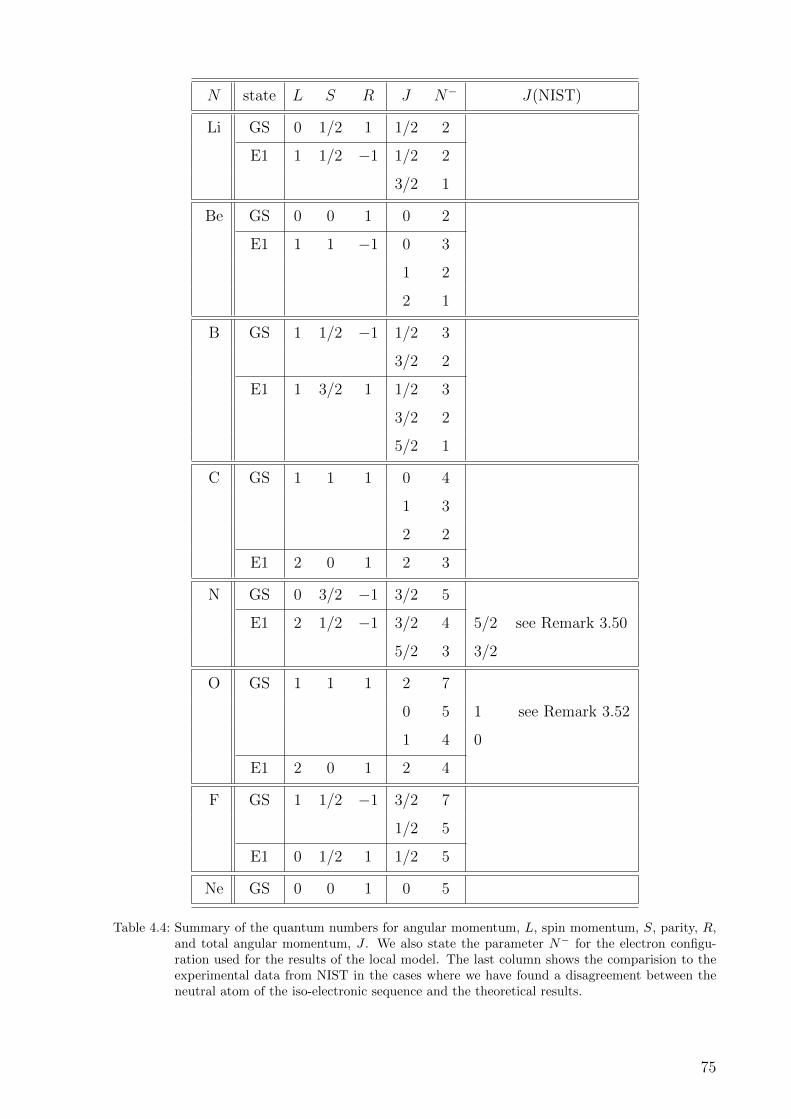
N state L S R J N− J(NIST)
Li GS 0 1/2 1 1/2 2
E1 1 1/2 −1 1/2 2
3/2 1
Be GS 0 0 1 0 2
E1 1 1 −1 0 3
1 2
2 1
B GS 1 1/2 −1 1/2 3
3/2 2
E1 1 3/2 1 1/2 3
3/2 2
5/2 1
C GS 1 1 1 0 4
1 3
2 2
E1 2 0 1 2 3
N GS 0 3/2 −1 3/2 5
E1 2 1/2 −1 3/2 4 5/2 see Remark 3.50
5/2 3 3/2
O GS 1 1 1 2 7
0 5 1 see Remark 3.52
1 4 0
E1 2 0 1 2 4
F GS 1 1/2 −1 3/2 7
1/2 5
E1 0 1/2 1 1/2 5
Ne GS 0 0 1 0 5
Table 4.4: Summary of the quantum numbers for angular momentum, L, spin momentum, S, parity, R,and total angular momentum, J . We also state the parameter N− for the electron configu-ration used for the results of the local model. The last column shows the comparision to theexperimental data from NIST in the cases where we have found a disagreement between theneutral atom of the iso-electronic sequence and the theoretical results.
75

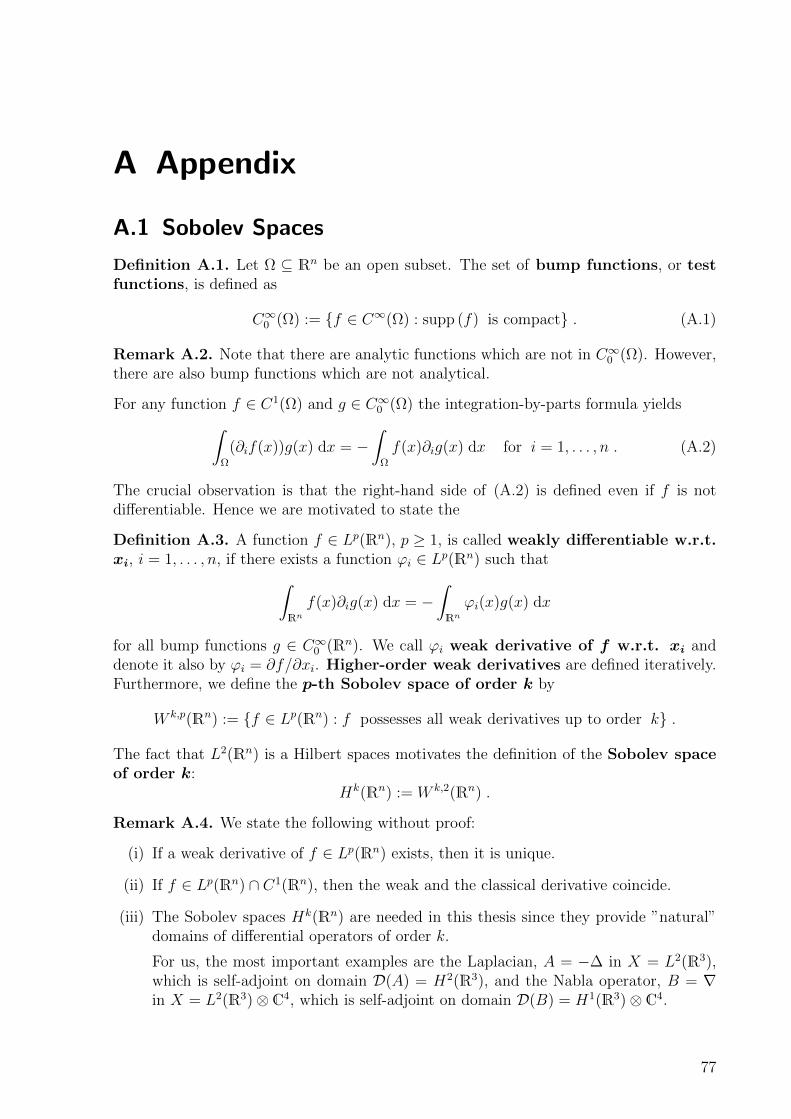
A Appendix
A.1 Sobolev Spaces
Definition A.1. Let Ω ⊆ Rn be an open subset. The set of bump functions, or testfunctions, is defined as
C∞0 (Ω) := f ∈ C∞(Ω) : supp (f) is compact . (A.1)
Remark A.2. Note that there are analytic functions which are not in C∞0 (Ω). However,there are also bump functions which are not analytical.
For any function f ∈ C1(Ω) and g ∈ C∞0 (Ω) the integration-by-parts formula yields∫Ω
(∂if(x))g(x) dx = −∫
Ω
f(x)∂ig(x) dx for i = 1, . . . , n . (A.2)
The crucial observation is that the right-hand side of (A.2) is defined even if f is notdifferentiable. Hence we are motivated to state the
Definition A.3. A function f ∈ Lp(Rn), p ≥ 1, is called weakly differentiable w.r.t.xi, i = 1, . . . , n, if there exists a function ϕi ∈ Lp(Rn) such that∫
Rnf(x)∂ig(x) dx = −
∫Rnϕi(x)g(x) dx
for all bump functions g ∈ C∞0 (Rn). We call ϕi weak derivative of f w.r.t. xi anddenote it also by ϕi = ∂f/∂xi. Higher-order weak derivatives are defined iteratively.Furthermore, we define the p-th Sobolev space of order k by
W k,p(Rn) := f ∈ Lp(Rn) : f possesses all weak derivatives up to order k .
The fact that L2(Rn) is a Hilbert spaces motivates the definition of the Sobolev spaceof order k:
Hk(Rn) := W k,2(Rn) .
Remark A.4. We state the following without proof:
(i) If a weak derivative of f ∈ Lp(Rn) exists, then it is unique.
(ii) If f ∈ Lp(Rn) ∩ C1(Rn), then the weak and the classical derivative coincide.
(iii) The Sobolev spaces Hk(Rn) are needed in this thesis since they provide ”natural”domains of differential operators of order k.
For us, the most important examples are the Laplacian, A = −∆ in X = L2(R3),which is self-adjoint on domain D(A) = H2(R3), and the Nabla operator, B = ∇in X = L2(R3)⊗ C4, which is self-adjoint on domain D(B) = H1(R3)⊗ C4.
77
A Appendix
Definition A.5. Let k, p ∈ N. For f ∈ C∞0 (Rn) the Sobolev norm || · ||k,p is defined as
||f ||k,p :=
∑|σ|≤k
n∑i=1
∣∣∣∣∣∣∣∣∂σif∂xσii
∣∣∣∣∣∣∣∣pp
1/p
, (A.3)
where σ ∈ Nn0 is a multiindex and |σ| := ∑n
i=1 σi = |σ|1.
Theorem A.6. The completion of the space of bump functions, C∞0 (Rn), w.r.t. theSobolev norm, || · ||k,p, is an alternative way to get the Sobolev spaces:
W k,p(Rn) = (C∞0 (Rn), || · ||k,p)||·||k,p
.
Proof. We refer to the literature, for instance [Eva98].
Remark A.7. Sometimes, for instance in [HS96], the Sobolev spaces are defined in thefirst place as completion of C∞0 (Rn).
For investigating the spectrum of the Dirac operator in section 2.2 we need a character-ization of the Sobolev space of order k, Hk(Rn), in terms of the Fourier transformation,or, more precisely, the Plancherel transformation:
Theorem A.8. Let k ∈ N and let P : L2(Rn)→ L2(Rn) denote the isometric Planchereltransformation. For a function f ∈ L2(Rn) the following statements are equivalent:
(i) f ∈ Hk(Rn) ,
(ii)(1 + |x|k
)Pf(x) ∈ L2(Rn) ,
(iii) (1 + |x|2)k/2Pf(x) ∈ L2(Rn) .
Proof. For the equivalence (i) ⇔ (ii) we refer to the literature, for instance [Eva98]. Theimplication (iii) ⇒ (ii) follows immediately. For the other direction (ii) ⇒ (iii) firstly weget
∫Rn|x|2k|Pf(x)| dx <∞. We derive
‖(1 + |x|2
)k/2Pf(x)‖22 =
∫Rn
(1 + |x|2
)k |Pf(x)|2 dx =
∫Rn
k∑l=0
(k
l
)|x|2l|Pf(x)|2 dx ≤
≤ Ck
∫Rnχ(|x| ≤ 1)|Pf(x)|2 dx+ Ck
∫Rnχ(|x| > 1)|x|2k|Pf(x)|2 dx ≤
≤ Ck
(||f ||22 +
∫Rn|x|2k|Pf(x)|2 dx
)<∞ ,
with a k-dependent finite number Ck := (k + 1) maxl=0,...k
(kl
). In the last line we have
used ||Pf ||2 = ||f ||2 <∞.
Remark A.9. The last Theorem A.8 offers the great possibility to extend the definitionof the Sobolev spaces Hk(Rn) also to non-integer values k ≥ 1. Therefore, one can definefor f ∈ L2(Rn): f ∈ Hπ(Rn) :⇔ (1 + |x|π)Pf(x) ∈ L2(Rn). For further reading we referto the literature, for instance [Tar07].
78
A.2 Spherical Harmonics and Laguerre Polynomials
A.2 Spherical Harmonics and Laguerre Polynomials
We consider Schrodinger operators H = −12∆ +V in L2(Rn) on a suitable domain D(H).
The potential V is some real-valued function on x ∈ R. In many physical application thepotential obeys some symmetry properties. They are, for instance, cylindrically symmet-ric, or, as the Coulomb potential V (x) = −Z/|x|, Z ∈ N, even spherically symmetric.Let us restrict to the Coulomb potential and the physical case n = 3. The main ideasof the following derivation can be found in physics textbooks, for instance in [Jac06] or[Sch07]. For classical reading we recommend [AS65].
We switch to the usual spherical coordinates x 7→ (r, θ, ϕ) ∈ [0,∞) × [0, π] × [0, 2π]which are suitable coordinates for isotropic systems. Making the factorization ansatz
ψ =U(r)
rP (θ)Q(ϕ) , (A.4)
and transforming the Laplacian into spherical coordinates, we find for the eigenvalueequation: [
−1
2(∆r + ∆θ,ϕ)− Z
r− E(r)
]U(r)
rP (θ)Q(ϕ) = 0 . (A.5)
The fact that the eigenvalue E(r) is a function only of the radial coordinate comes fromthe spherical symmetry of the Coulomb interaction. We have separated the Laplacianinto a radial, ∆r, and a spherical part, ∆θ,ϕ, with ∆ = ∆r + ∆θ,ϕ:
∆r :=1
r∂2r r =
1
r∂r r ∂r +
1
r∂r = ∂2
r +2
r∂r,
∆θ,ϕ :=1
r2 sin θ∂θ(sin θ ∂θ) +
1
r2 sin2 θ∂2ϕ .
(A.6)
A.2.1 Spherical Harmonics
First we concentrate on the angular part of this equation and consider the Laplace equa-tion
∆ψ = (∆r + ∆θ,ϕ)U(r)
rP (θ)Q(ϕ) = 0 . (A.7)
For ψ 6= 0 this is equivalent to
r2 sin2 θ
U(r)∂2r U(r) +
sin θ
P (θ)∂θ(sin θ ∂θ)P (θ) +
1
Q(ϕ)∂2ϕQ(ϕ) = 0 . (A.8)
Only the third term depends only on ϕ, hence it must be a constant c2 ∈ R:
∂2ϕQ(ϕ) = c2Q(ϕ) ⇒ Q(ϕ) = exp(cϕ) . (A.9)
The periodic boundary condition ψ(·, ·, ϕ) = ψ(·, ·, ϕ + 2π) implies exp(2πc) = 1. Thismeans c ∈ iZ. Therefore we introduce a new constant1 m := −ic ∈ Z, thus
Qm(ϕ) = exp(imϕ) . (A.10)
1This constant m is called magnetic quantum number.
79
A Appendix
Plugging this into (A.8) and dividing by sin2 θ yields:
r2
U(r)∂2r U(r) +
1
sin θ P (θ)∂θ(sin θ ∂θ)P (θ)− m2
sin2 θ= 0 . (A.11)
Only the first term depends only on r. Furthermore, only the second and third termdepends only on θ. Therefore, the first term must be a constant, C ∈ R, and the secondand third term must be the same constant with opposite sign. We arrive at:(
∂2r −
C
r2
)U(r) = 0 ,[
1
sin θ∂θ(sin θ ∂θ) +
(C − m2
sin2 θ
)]P (θ) = 0 .
(A.12)
The differential equation for P is well-known in mathematical physics. We switch tox := cos θ ∈ [−1, 1] and meet the general Legendre equation:[
d
dx
((1− x2)
d
dx
)+
(C − m2
1− x2
)]P (x) = 0 . (A.13)
For m = 0 this equation is called Legendre equation. This case relates to a Q(ϕ) = 1and describes systems with azimuthal symmetry. We address now this case and make for−1 ≤ x ≤ 1 the following power-series ansatz:
P (x) = xα∞∑j=0
ajxj , (A.14)
with aj ∈ R α ∈ R. We have the following
Lemma A.10. Assuming that (A.14) is a solution of the Legendre equation, (A.13) form = 0, one has:
(a) a0 6= 0⇒ α ∈ 0, 1 and a1 6= 0⇒ α ∈ −1, 0 .
(b) For j ≥ 2, the coefficients are recursively given by
aj = aj−2 ·(α + j − 2)(α + j − 1)− C
(α + j − 1)(α + j).
In particular: a0 = 0⇒ a2n = 0 ∀n ∈ N and a1 = 0⇒ a2n+1 = 0 ∀n ∈ N.
(c) P (x) is convergent for all −1 < x < 1.
(d) P (x) is convergent for |x| = 1⇔ C = l(l + 1) for some l ∈ N0.
(e) In the case of (d): α = 0⇔ l is even, α = 1⇔ l is odd.
Proof. The ideas of the proof can be found in [Jac06] and the references therein.
Remark A.11. The decomposition of the constant C = l(l+1) is crucial for the physicalinterpretation2. As the Lemma tells us, it is necessarily that l ∈ N0 in order to make
2This constant l is called angular momentum quantum number.
80
A.2 Spherical Harmonics and Laguerre Polynomials
the power series convergent at x ∈ −1, 1. In this case, the power series reduces to apolynomial function with only odd or even powers of x. They can be cataloged by l. Wefollow the usual convention and normalize these Legendre polynomials by Pl(1) = 1.
Theorem A.12.
(a) The Legendre polynomials (l ∈ N0) are given by Rodrigues’ formula:
Pl(x) =1
2l l!
dl
dxl(x2 − 1)l . (A.15)
(b) The set ⋃l∈N0
Ul : [−1, 1]→ R, Ul(x) :=
√2l + 1
2Pl(x)
is a orthonormal basis of the Hilbert space (L2([−1, 1]), 〈· , ·〉) with 〈Ul, Uk〉 = δl,k.
For a given l ∈ N0 we restrict the constant m ∈ Z to m = 0, 1, . . . , l and define theassociated Legendre polynomials Pm
l : [−1, 1]→ R by
Pml (x) := (−1)m(1− x2)m/2
dm
dxmPl(x) . (A.16)
Theorem A.13.
(a) The associated Legendre polynomials (l ∈ N0, m = 0,±1, . . . ,±l) are given byRodrigues’ formula:
Pml (x) =
(−1)m
2l l!(1− x2)m/2
dl+m
dxl+m(x2 − 1)l . (A.17)
(b) The polynomials with negative m are proportional to those with positive m:
P−|m|l (x) = (−1)|m|
(l − |m|)!(l + |m|)!P
|m|l . (A.18)
(c) The associated Legendre polynomials Pml (l ∈ N0, m = −l,−l + 1, . . . , l − 1, l) are
solutions of the general Legendre equation (A.13).
(d) The set ⋃l∈N0
Uml : [−1, 1]→ R, Ul(x) :=
√2l + 1
2
(l −m)!
(l +m)!Pml (x)
is for all m = −l,−l + 1, . . . , l − 1, l an orthonormal basis of the Hilbert space(L2([−1, 1]), 〈· , ·〉) with 〈Um
l , Umk 〉 = δl,k.
We have already found the solutions Qm(ϕ) = exp(imϕ), m ∈ Z, of the azimuthal angle(A.10). As we know, the set⋃
m∈Z
Um : [0, 2π]→ C, Um(ϕ) =1√2π
exp(imϕ) (A.19)
81
A Appendix
forms an orthonormal basis of the Hilbert space (L2([−1, 1]), 〈· , ·〉) with 〈Um, Un〉 = δm,n.Therefore, the product of the Legendre polynomials Pm
l (cos θ) and the functions Qm(ϕ)(with the corresponding prefactors) form a basis of square-integrable functions on thesurface of a sphere: we define the spherical harmonics Ylm : R2 → C by
Ylm(θ, ϕ) :=1√2π
√2l + 1
2
(l −m)!
(l +m)!Pml (cos θ)eimϕ , (A.20)
again for l ∈ N0 and m = −l,−l + 1, . . . , l − 1, l.
Remark A.14. The prefactors and the orthogonality of both, Pml and Qm, imply that
the spherical harmonics fulfill: 〈Ylm, Ykn〉 = δlkδmn. Furthermore, Ylm(θ + π, ϕ + 2π) =(−1)l+mYlm(θ, ϕ). The periodicity of ϕ is obvious. The changing sign comes from theidentity Pm
l (−x) = (−1)l+mPml (x), which is clear from (A.15) and (A.16).
A.2.2 Laguerre Polynomials
We concentrate now on the radial part of (A.5). Since the Coulomb potential is onlynegative, V (r) = −Z/r < 0, we investigate this eigenvalue equation for E < 03. Usingthe result that P (θ)Q(ϕ) = Ylm(θ, ϕ) are eigenfunctions of the spherical Laplacian, ∆θ,ϕ,with eigenvalue −C/r2 = −l(l + 1)/r2, (A.5) reads:[
−1
2∂2r +
l(l + 1)
2r2− Z
r+ |E|
]u(r) = 0 , (A.21)
for a function u : [0 ,∞)→ R. We have used the first form of the radial Laplacian (A.6).We follow the calculation in [Sch07] and switch to the following quantities:
ρ :=√
2|E|r and ρ0 :=2Z√2|E|
⇒ V
|E| = −ρ0
ρ. (A.22)
Therefore, the eigenvalue equation (A.21) reads:[∂2ρ −
l(l + 1)
ρ2+
ρ
ρ0
− 1
]u(ρ) = 0 . (A.23)
As in the discussion of the spherical part of the Laplacian, we make a power-series ansatz:
u(ρ) = ρl+1e−ρ∞∑k=0
akρk . (A.24)
The condition, that the solution is not exponentially divergent for large ρ, i.e. for large r,implies that there must be some N ∈ N0 such that4 ρ0 = 2(N + l + 1) =: 2n. Thereforen ∈ N and l = 0, 1, . . . , n − 1. From this, we can catalog the eigenvalues by n and find
3Indeed, for E ≥ 0 this eigenvalue equation has no solution. This follows from the fact that σess(H) =[0 ,∞) (see Theorem 2.36), hence E ≥ 0 cannot be an eigenvalue.
4The constant N is called radial quantum number and the constant n is called principal quantumnumber.
82
A.2 Spherical Harmonics and Laguerre Polynomials
directly from (A.22):
|E| = −V ρρ0
=Z√
2|E|r2nr
⇒ 0 > E = − Z2
2n2. (A.25)
For the eigenfunction we consider the general Laguerre equation for Lsr : [0 ,∞)→ R:[x∂2
x + (s+ 1− x)∂x + (r − s)]Lsr(x) = 0 . (A.26)
For s = 0 this equation is called Laguerre equation. We have the following
Theorem A.15.
(a) The associated Laguerre polynomials, Lsr, given by Rodrigues’ formula5
Lsr(x) =ex x−s
(r − s)!dr−s
dxr−sex(e−xxr
),
with r, s ∈ N0, r ≥ s, are solutions of the general Laguerre equation.
(b) Furthermore, the associated Laguerre polynomials are given explicitly by
Lsr(x) =r−s∑k=0
(−1)k(r!)xk
k!(k + s)!(r − k − s)! .
(c) For the normalization one has∫ ∞0
xs+1 e−x [Lsr(x)]2 dx =(2r − s+ 1)(r!)
(r − s)! .
Finally we can state the solution for (A.21) and, what was the claim of this whole section,for (A.5). Ylm denote the spherical harmonics and Lsr denote the associated Laguerrepolynomials.
Theorem A.16. The eigenvalue equation (A.5) with eigenvalue En = −Z2/2n2 < 0 issolved by ψnlm : [0 ,∞)× [0, π]× [0, 2π]→ C with
ψnml(r, θ, ϕ) = Z3/2Rnl(Zr)Ylm(θ, ϕ) ,
where n ∈ N0, l = 0, 1, . . . , n− 1 and m = −l,−l+ 1, . . . , l− 1, l are admissible. Therebywe have defined
Rnl(r) :=U(r)
r=
2
n2
√(n− l − 1)!
(n+ l)!e−r/n
(2r
n
)lL2l+1n+l (2r/n) .
5In the literature there are several conventions for the Laguerre polynomials. Quite frequently they aredenoted by Lk
n(x), with n, k ∈ N0, k ≤ n. These functions coincide with those in our convention whenidentifying s↔ k and n↔ r − s.
83
A Appendix
The l,m–dependent prefactor of Rnl(r) is due to the normalization of Lsr. We want toemphasize at this point, that Rnl(r) is independent of the magnetic quantum number m.Furthermore, expressing the spherical symmetry of the Coulomb potential, the energyeigenvalues En < 0 depend only on the principal quantum number n. However, wehave defined the solutions ψnlm in spherical coordinates. Transforming back to Cartesiancoordinates, these eigenfunctions are functions on R3 and, indeed, square integrable.
A.3 Notations in Relativistic Quantum Mechanics
The Pauli matrices σi, for i = 1, 2, 3, are defined as
σ1 =
(0 11 0
), σ2 =
(0 −ii 0
), σ3 =
(1 00 −1
). (A.27)
All Pauli matrices are traceless, traceσi = 0, and hermitian, σ†i := σT∗i = σi. Even more,
any traceless hermitian 2× 2 matrix can be written as some unique linear combination ofthe Pauli matrices.
The Pauli matrices obey the following commutator relation: [σi, σj] = 2iεijkσk, whereεijk denotes the totally antisymmetric tensor
εijk =
1 (ijk) = (123) or any cyclic permutation,−1 (ijk) = (213) or any cyclic permutation,0 else.
(A.28)
In physics they are closely related to spin-12-particles: the operator describing their spin
angular momentum is given by S = 12σ, compare Definition 3.2. When describing rela-
tivistic Dirac spinors in C4 instead of non-relativistic Weyl spinors in C2, the spin operator
reads S ⊗ 12 = 12
(σ 00 σ
)=: 1
2Σ.
From a group-theoretic point of view, the Pauli matrices are just the infinitesimal gen-erators of the three-dimensional Lie group SU(2). For this enlightening branch of grouptheory we refer to the literature, for instance [FH91] and many physics textbooks. Impor-tant results are Stone’s Theorem, discussed in [RS75], and Nelson’s Theorem, discussedin [Tha92].
84
Bibliography
[AS65] M. Abramowitz and I. A. Stegun. Handbook of Mathematical Functions withFormulas, Graphs, and Mathematical Tables. Dover, 1965.
[CHD05] N. G. Connelly, R. M. Hartshorn, and T. Damhus. Nomenclature of InorganicChemistry: IUPAC Recommendations 2005. Royal Society of Chemistry, 2005.
[Eva98] L. C. Evans. Partial Differential Equations. American Mathematical Society,1998.
[FG09a] G. Friesecke and B. D. Goddard. Asymptotics-Based CI Models for Atoms:Properties, Exact Solution of a Minimal Model for Li to Ne, and Application toAtomic Spectra. Multiscale Modeling & Simulation, 7(4):1876–1897, 2009.
[FG09b] G. Friesecke and B. D. Goddard. Explicit large nuclear charge limit of electronicground states for Li, Be, B, C, N, O, F, Ne and basic aspects of the periodic table.SIAM Journal on Mathematical Analysis, 41:631–664, 2009.
[FG10] G. Friesecke and B. D Goddard. Atomic structure via highly charged ions andtheir exact quantum states. Physical Review A, 81:032516, 2010.
[FH91] W. Fulton and J. Harris. Representation Theory. Springer, 1991.
[Fri03] G. Friesecke. The Multiconfiguration Equations for Atoms and Molecules: ChargeQuantization and Existence of Solutions. Archive for Rational Mechanics andAnalysis, 169(1):35–75, 2003.
[Fri07] G. Friesecke. Quantum Mechanics for Mathematicians. Lecture notes, 2007.
[GGM03] F. Gazzola, H. Ch. Grunau, and E. Mitidieri. Hardy Inequalities with OptimalConstants and Remainder Terms. Transactions of the American MathematicalSociety, 356(6):2149–2168, 2003.
[HS96] P. D. Hislop and I. M. Sigal. Introduction to Spectral Theory with Applicationsto Schrodinger Operators. Springer, 1996.
[Jac06] J. D. Jackson. Klassische Elektrodynamik. de Gruyter, 2006.
[Jen06] F. Jensen. Introduction to Computational Chemistry. Wiley, 2006.
[Kan09] E. Kaniuth. A Course in Commutative Banach Algebras. Springer, 2009.
[N+10] K. Nakamura et al. Review of Particle Physics. Journal of Physics G, 37:075021,2010.
[Pau40] W. Pauli. The Connection between Spin and Statistics. Physical Review,58(8):716–722, 1940.
85
Bibliography
[Per83] P. A. Perry. Scattering Theory by the Enss Method. Mathematical Reports, 1983.
[PS95] M. E. Peskin and D. V. Schroeder. An Introduction to Quantum Field Theory.Westview Press, 1995.
[RS75] M. Reed and B. Simon. II - Fourier Analysis, Self-adjointness. Elsevier, 1975.
[RS78] M. Reed and B. Simon. IV - Analysis of Operators. Elsevier, 1978.
[RS80] M. Reed and B. Simon. I - Functional Analysis. Elsevier, 1980.
[Rud91] W. Rudin. Functional Analysis. McGraw-Hill, 1991.
[Sch05] F. Schwabl. Quantenmechanik fur Fortgeschrittene. Springer, 2005.
[Sch07] F. Schwabl. Quantenmechanik. Springer, 2007.
[Tar07] L. Tartar. An Introduction to Sobolev Spaces and Interpolation Spaces. Springer,2007.
[Tha92] B. Thaller. The Dirac Equation. Springer, 1992.
[Ves69] K. Veselic. The nonrelativistic limit of the Dirac equation and the spectral con-centration. Glasnik Mathematicki, 4:231–240, 1969.
[Yu.10] Yu. Ralchenkom, F.-C. Jou, D. E. Kelleher, A. E. Kramida, A. Musgrove, J.Reader, W. L. Wiese, and K. Olsen. NIST Atomic Spectra Database (version4.0.1) [Online], 2010. Available: http://physics.nist.gov/asd.
86
Acknowledgement
In these final lines I try to express my gratitude to all the people who have supportedme during my studies and particularly during the last six months when working on thisthesis.
During more than five years Prof. Dr. Gero Friesecke has taught me in many lecturesand discussions in both mathematics and physics: at the beginning in the elementarycalculus courses, later on in lectures which have combined abstract mathematical formal-ism and problems arising in physics. I have learnt from him that mathematics which isapplied to physical questions helps to learn more about both issues. I am very thankfulto Prof. Friesecke for his confidence in me and for asking me to work on the perturbationtheory model in this diploma thesis and in the prior project thesis. I also thank you forthe opportunity to attend the workshop at Oberwolfach about “Mathematical Methodsin Quantum Chemistry” in the upcoming month.
During my whole studies I have been accompanied by Stefan Kahler. At the beginningI have known him as a fellow student, then it emerged that we are indeed neighbors, andactually we have become friends. During many night sessions we have discussed problemsarising not only in mathematics or physics and have learnt from each other. Thank youfor all your support, especially for preparing and testing me for upcoming exams and forproofreading my diploma thesis.
I know that I am repeating myself, but, really, it is impossible to write a diploma thesiswithin isolation! Also during my official absence at T39 in the last six months I havefound here always an open door for discussions and meetings. Thank you all very muchfor your support.
Auch wenn ich eine etwas andere Meinung zur Schule, insbesondere zur Mathematik,vertrete, so danke ich Reinhard Mey fur seine wunderbaren Texte, Melodien und Gedanken.Beinahe taglich begleiten sie mich; real oder oft auch rein imaginar.
Last but not least I am indebted to my parents and my sister. Everything I have reachedso far in my life I owe to my family. They have provided a comfortable environment I wasalways able to pursue intensely my interests.
87


![MPA Lecture on Numerical Methods for Cosmologykomatsu/lecturenotes/...relativistic numerical methods already exist [see e.g. 3, 6]. In any case rela-tivistic e ects only a ect the](https://img.pdfslide.us/doc/110x75/5fc398d52bb21d53085e8faa/mpa-lecture-on-numerical-methods-for-cosmology-komatsulecturenotes-relativistic.jpg)