Embed Size (px)
Citation preview
Relativistic effects in Physics andAstrophysics

Contents
1. Topics 1871
2. Participants 18732.1. ICRANet participants . . . . . . . . . . . . . . . . . . . . . . . . 18732.2. Past collaborators . . . . . . . . . . . . . . . . . . . . . . . . . . 1873
3. Brief description 18753.1. Highlights of new results . . . . . . . . . . . . . . . . . . . . . . 1875
3.1.1. The luminosity evolution over the EQTSs in the GRBprompt emission . . . . . . . . . . . . . . . . . . . . . . 1875
3.1.2. The apparent size of EQTSs in the sky . . . . . . . . . . 18773.2. Appendix on previous results . . . . . . . . . . . . . . . . . . . 1877
3.2.1. Exact vs. approximate solutions in GRB afterglows . . 18773.2.2. Exact analytic expressions for the EQTSs in GRBs . . . 18773.2.3. Exact vs. approximate beaming formulas in GRBs . . . 1878
4. Publications on refereed journals 1879
A. The luminosity evolution over the EQTSs in the GRB prompt emis-sion 1881A.1. The Equitemporal surfaces (EQTS) . . . . . . . . . . . . . . . . 1881A.2. The extended afterglow luminosity distribution over the EQTS 1883A.3. Conclusions . . . . . . . . . . . . . . . . . . . . . . . . . . . . . 1883
B. The EQTS apparent radius in the sky 1887B.1. Conclusions . . . . . . . . . . . . . . . . . . . . . . . . . . . . . 1892
C. Exact vs. approximate solutions in GRB afterglows 1893C.1. Differential formulation of the afterglow dynamics equations . 1893C.2. The exact analytic solutions . . . . . . . . . . . . . . . . . . . . 1894C.3. Approximations adopted in the current literature . . . . . . . 1895
C.3.1. The fully radiative case . . . . . . . . . . . . . . . . . . 1896C.3.2. The adiabatic case . . . . . . . . . . . . . . . . . . . . . 1897
C.4. A specific example . . . . . . . . . . . . . . . . . . . . . . . . . 1898
D. Exact analytic expressions for the EQTSs in GRB afterglows 1901D.1. The definition of the EQTSs . . . . . . . . . . . . . . . . . . . . 1901
1869
Contents
D.2. The analytic expressions for the EQTSes . . . . . . . . . . . . . 1906D.2.1. The fully radiative case . . . . . . . . . . . . . . . . . . 1906D.2.2. The adiabatic case . . . . . . . . . . . . . . . . . . . . . 1906D.2.3. Comparison between the two cases . . . . . . . . . . . 1906
D.3. Approximations adopted in the current literature . . . . . . . 1908
E. Exact vs. approximate beaming formulas in GRB afterglows 1913E.1. Analytic formulas for the beaming angle . . . . . . . . . . . . . 1914
E.1.1. The fully radiative regime . . . . . . . . . . . . . . . . . 1914E.1.2. The adiabatic regime . . . . . . . . . . . . . . . . . . . . 1915E.1.3. The comparison between the two solutions . . . . . . . 1915
E.2. Comparison with the existing literature . . . . . . . . . . . . . 1917E.3. An empirical fit of the numerical solution . . . . . . . . . . . . 1919
Bibliography 1921
1870
1. Topics
• The Gamma-Ray Burst (GRB) extended afterglow luminosity evolutionover the equitemporal surfaces (EQTS).
• The apparent radius of the equitemporal surfaces in the sky.
• Exact versus approximate equations of motion in GRB afterglows.
• Exact analytic expressions for the EQTS in GRB afterglows.
• Exact versus approximate beaming formulas in GRB afterglows.
1871


2. Participants
2.1. ICRANet participants
• Carlo Luciano Bianco
• Remo Ruffini
2.2. Past collaborators
• Christian Cherubini (Universita “Campus Biomedico”, Italy)
• Jurgen Ehlers (Max-Plank Institut, Germany)
• Federico Fraschetti (CEA Saclay, France)
• Eliana La Francesca (Undergraduate, Italy)
• Francesco Alessandro Massucci (Undergraduate, Italy)
1873

3. Brief description
3.1. Highlights of new results
3.1.1. The luminosity evolution over the equitemporalsurfaces in the prompt emission of Gamma-Ray Bursts
It is widely accepted that Gamma-Ray Burst (GRB) afterglows originate fromthe interaction of an ultrarelativistically expanding shell into the CircumBurstMedium (CBM). Differences exists on the detailed kinematics and dynamicsof such a shell (see e.g. Bianco and Ruffini, 2005a; Meszaros, 2006, and refs.therein).
Due to the ultrarelativistic velocity of the expanding shell (Lorentz gammafactor γ ∼ 102 − 103), photons emitted at the same time in the laboratoryframe (i.e. the one in which the center of the expanding shell is at rest) fromthe shell surface but at different angles from the line of sight do not reachthe observer at the same arrival time. Therefore, if we were able to resolvespatially the GRB afterglows, we would not see the spherical surface of theshell. We would see instead the projection on the celestial sphere of the EQ-uiTemporal Surface (EQTS), defined as the surface locus of points which aresource of radiation reaching the observer at the same arrival time (see e.g.Couderc, 1939; Rees, 1966; Sari, 1998; Panaitescu and Meszaros, 1998; Gra-not et al., 1999a; Bianco et al., 2001; Bianco and Ruffini, 2004, 2005b, and refs.therein). The knowledge of the exact shape of the EQTSs is crucial, since anytheoretical model must perform an integration over the EQTSs to computeany prediction for the observed quantities (see e.g. Gruzinov and Waxman,1999; Oren et al., 2004; Bianco and Ruffini, 2004, 2005b; Granot et al., 2005;Meszaros, 2006; Huang et al., 2006, 2007, and refs. therein).
One of the key problems is the determination of the angular size of the vis-ible region of each EQTS, as well as the distribution of the luminosity oversuch a visible region. In the current literature it has been shown that in thelatest afterglow phases the luminosity is maximum at the boundaries of thevisible region and that the EQTS must then appear as expanding luminous“rings” (see e.g. Waxman, 1997; Sari, 1998; Panaitescu and Meszaros, 1998;Granot et al., 1999a,b; Waxman et al., 1998; Galama et al., 2003; Granot andLoeb, 2003; Taylor et al., 2004; Granot, 2008, and refs. therein). Such an anal-ysis is applied only in the latest afterglow phases to interpret data from radioobservations (Frail et al., 1997; Waxman et al., 1998; Galama et al., 2003; Tay-
1875
3. Brief description
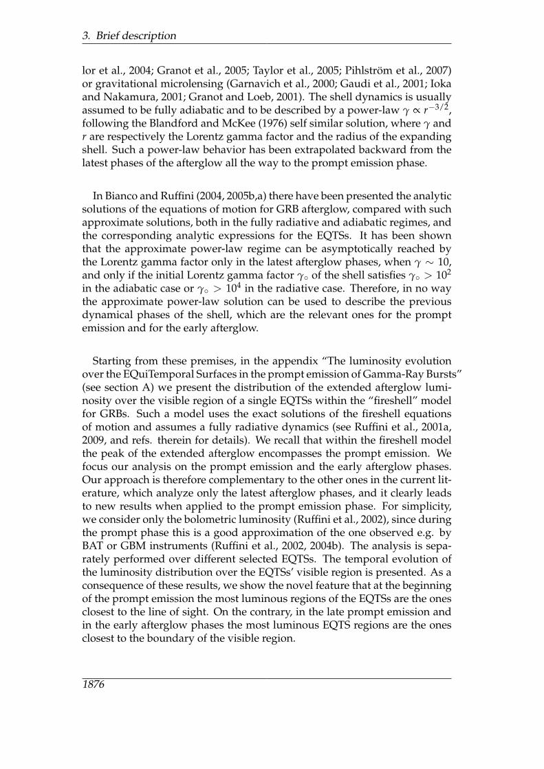
lor et al., 2004; Granot et al., 2005; Taylor et al., 2005; Pihlstrom et al., 2007)or gravitational microlensing (Garnavich et al., 2000; Gaudi et al., 2001; Iokaand Nakamura, 2001; Granot and Loeb, 2001). The shell dynamics is usuallyassumed to be fully adiabatic and to be described by a power-law γ ∝ r−3/2,following the Blandford and McKee (1976) self similar solution, where γ andr are respectively the Lorentz gamma factor and the radius of the expandingshell. Such a power-law behavior has been extrapolated backward from thelatest phases of the afterglow all the way to the prompt emission phase.
In Bianco and Ruffini (2004, 2005b,a) there have been presented the analyticsolutions of the equations of motion for GRB afterglow, compared with suchapproximate solutions, both in the fully radiative and adiabatic regimes, andthe corresponding analytic expressions for the EQTSs. It has been shownthat the approximate power-law regime can be asymptotically reached bythe Lorentz gamma factor only in the latest afterglow phases, when γ ∼ 10,and only if the initial Lorentz gamma factor γ of the shell satisfies γ > 102
in the adiabatic case or γ > 104 in the radiative case. Therefore, in no waythe approximate power-law solution can be used to describe the previousdynamical phases of the shell, which are the relevant ones for the promptemission and for the early afterglow.
Starting from these premises, in the appendix “The luminosity evolutionover the EQuiTemporal Surfaces in the prompt emission of Gamma-Ray Bursts”(see section A) we present the distribution of the extended afterglow lumi-nosity over the visible region of a single EQTSs within the “fireshell” modelfor GRBs. Such a model uses the exact solutions of the fireshell equationsof motion and assumes a fully radiative dynamics (see Ruffini et al., 2001a,2009, and refs. therein for details). We recall that within the fireshell modelthe peak of the extended afterglow encompasses the prompt emission. Wefocus our analysis on the prompt emission and the early afterglow phases.Our approach is therefore complementary to the other ones in the current lit-erature, which analyze only the latest afterglow phases, and it clearly leadsto new results when applied to the prompt emission phase. For simplicity,we consider only the bolometric luminosity (Ruffini et al., 2002), since duringthe prompt phase this is a good approximation of the one observed e.g. byBAT or GBM instruments (Ruffini et al., 2002, 2004b). The analysis is sepa-rately performed over different selected EQTSs. The temporal evolution ofthe luminosity distribution over the EQTSs’ visible region is presented. As aconsequence of these results, we show the novel feature that at the beginningof the prompt emission the most luminous regions of the EQTSs are the onesclosest to the line of sight. On the contrary, in the late prompt emission andin the early afterglow phases the most luminous EQTS regions are the onesclosest to the boundary of the visible region.
1876
3.2. Appendix on previous results
3.1.2. The apparent size of equitemporal surfaces in the sky
A consequence of the results presented above is that we were able to derive ananalytic expression for the temporal evolution, measured in arrival time, ofthe apparent size of the EQTSs in the sky, valid in both the fully radiative andthe adiabatic regimes. Such an expression is presented in the appendix “Theapparent radius of the equitemporal surfaces in the sky” (section B). We willalso discuss analogies and differences with other approaches in the currentliterature which assumes an adiabatic dynamics instead of a fully radiativeone.
3.2. Appendix on previous results
3.2.1. Exact versus approximate solutions in Gamma-RayBurst afterglows
In the appendix “Exact versus approximate solutions in Gamma-Ray Burstafterglows” (section C) we first write the energy and momentum conserva-tion equations for the interaction between the ABM pulse and the Circum-Burst Medium (CBM) in a finite difference formalism, already discussed inthe previous report about “Gamma-Ray Bursts”. We then express these sameequations in a differential formalism to compare our approach with the onesin the current literature. We write the exact analytic solutions of such dif-ferential equations both in the fully radiative and in the adiabatic regimes.We then compare and contrast these results with the ones following fromthe ultra-relativistic approximation widely adopted in the current literature.Such an ultra-relativistic approximation, adopted to apply to Gamma-RayBursts (GRBs) the Blandford and McKee (1976) self-similar solution, led toa simple power-law dependence of the Lorentz gamma factor of the bary-onic shell on the distance. On the contrary, we show that no constant-indexpower-law relations between the Lorentz gamma factor and the distance canexist, both in the fully radiative and in the adiabatic regimes. The exact solu-tion is indeed necessary if one wishes to describe properly all the phases ofthe afterglow including the prompt emission.
3.2.2. Exact analytic expressions for the equitemporalsurfaces in Gamma-Ray Burst afterglows
In the appendix “Exact analytic expressions for the equitemporal surfaces inGamma-Ray Burst afterglows” (section D) we follow the indication by PaulCouderc (1939) who pointed out long ago how in all relativistic expansionsthe crucial geometrical quantities with respect to a physical observer are the“equitemporal surfaces” (EQTSs), namely the locus of source points of the
1877
3. Brief description
signals arriving at the observer at the same time. After recalling the formaldefinition of the EQTSs, we use the exact analytic solutions of the equationsof motion recalled in the previous section to derive the exact analytic expres-sions of the EQTSs in GRB afterglow both in the fully radiative and adiabaticregimes. We then compare and contrast such exact analytic solutions with thecorresponding ones widely adopted in the current literature and computedusing the approximate “ultra-relativistic” equations of motion discussed inthe previous section. We show that the approximate EQTS expressions leadto uncorrect estimates of the size of the ABM pulse when compared to theexact ones. Quite apart from their academic interest, these results are crucialfor the interpretation of GRB observations: all the observables come in factfrom integrated quantities over the EQTSs, and any minor disagreement intheir definition can have extremely drastic consequences on the identificationof the true physical processes.
3.2.3. Exact versus approximate beaming formulas inGamma-Ray Burst afterglows
In the appendix “Exact versus approximate beaming formulas in Gamma-Ray Burst afterglows” (section E) we discuss the possibility that GRBs origi-nate from a beamed emission, one of the most debated issue about the natureof the GRB sources in the current literature after the work by Mao and Yi(1994) (see e.g. Piran, 2005; Meszaros, 2006, and references therein). In par-ticular, on the ground of the theoretical considerations by Sari et al. (1999), itwas conjectured that, within the framework of a conical jet model, one mayfind that the gamma-ray energy released in all GRBs is narrowly clusteredaround 5 × 1050 ergs (Frail et al., 2001). We have never found in our GRBmodel any necessity to introduce a beamed emission. Nevertheless, we haveconsidered helpful and appropriate helping the ongoing research by givingthe exact analytic expressions of the relations between the detector arrivaltime td
a of the GRB afterglow radiation and the corresponding half-openingangle ϑ of the expanding source visible area due to the relativistic beaming.We have done this both in the fully radiative and in the adiabatic regimes, us-ing the exact analytic solutions presented in the previous sections. Again, wehave compared and contrasted our exact solutions with the approximate oneswidely used in the current literature. We have found significant differences,particularly in the fully radiative regime which we consider the relevant onefor GRBs, and it goes without saying that any statement on the existence ofbeaming can only be considered meaningful if using the correct equations.
1878
4. Publications on refereed journals
1. C.L. Bianco, R. Ruffini; “Exact versus approximate equitemporal sur-faces in Gamma-Ray Burst afterglows”; The Astrophysical Journal, 605,L1 (2004).
By integrating the relativistic hydrodynamic equations introduced by Taub wehave determined the exact EQuiTemporal Surfaces (EQTSs) for the Gamma-Ray Burst (GRB) afterglows. These surfaces are compared and contrasted tothe ones obtained, using approximate methods, by Panaitescu and Meszaros(1998); Sari (1998); Granot et al. (1999a).
2. C.L. Bianco, R. Ruffini; “On the exact analytic expressions for the equi-temporal surfaces in Gamma-Ray Burst afterglows”; The AstrophysicalJournal, 620, L23 (2005).
We have recently shown (see Bianco and Ruffini, 2004) that marked differencesexist between the EQuiTemporal Surfaces (EQTSs) for the Gamma-Ray Burst(GRB) afterglows numerically computed by the full integration of the equa-tions of motion and the ones found in the current literature expressed ana-lytically on the grounds of various approximations. In this Letter the exactanalytic expressions of the EQTSs are presented both in the case of fully ra-diative and adiabatic regimes. The new EQTS analytic solutions validate thenumerical results obtained in Bianco and Ruffini (2004) and offer a powerfultool to analytically perform the estimates of the physical observables in GRBafterglows.
3. C.L. Bianco, R. Ruffini; “Exact versus approximate solutions in Gamma-Ray Burst afterglows”; The Astrophysical Journal, 633, L13 (2005).
We have recently obtained the exact analytic solutions of the relativistic equa-tions relating the radial and time coordinate of a relativistic thin uniform shellexpanding in the interstellar medium in the fully radiative and fully adiabaticregimes. We here re-examine the validity of the constant-index power-law re-lations between the Lorentz gamma factor and its radial coordinate, usuallyadopted in the current Gamma-Ray Burst (GRB) literature on the grounds ofan “ultrarelativistic” approximation. Such expressions are found to be math-ematically correct but only approximately valid in a very limited range of thephysical and astrophysical parameters and in an asymptotic regime which isreached only for a very short time, if any, and are shown to be not applicableto GRBs.
1879
4. Publications on refereed journals
4. C.L. Bianco, R. Ruffini; “Exact versus approximate beaming formulaein Gamma-Ray Burst afterglows”; The Astrophysical Journal, 644, L105(2006).
We present the exact analytic expressions to compute, assuming the emittedGamma-Ray Burst (GRB) radiation is not spherically symmetric but is con-fined into a narrow jet, the value of the detector arrival time at which we startto “see” the sides of the jet, both in the fully radiative and adiabatic regimes.We obtain this result using our exact analytic expressions for the EQuiTempo-ral Surfaces (EQTSs) in GRB afterglows. We re-examine the validity of threedifferent approximate formulas currently adopted for the adiabatic regime inthe GRB literature. We also present an empirical fit of the numerical solu-tions of the exact equations, compared and contrasted with the three aboveapproximate formulas. The extent of the differences is such as to require a re-assessment on the existence and entity of beaming in the cases considered inthe current literature, as well as on its consequences on the GRB energetics.
5. C.L. Bianco, F.A. Massucci, R. Ruffini: “The luminosity evolution overthe EQuiTemporal Surfaces in the prompt emission of Gamma-Ray Bursts”;The Astrophysical Journal, submitted (2009).
Due to the ultrarelativistic velocity of the expanding “fireshell” (Lorentz gammafactor γ ∼ 102 − 103), photons emitted at the same time from the fireshellsurface do not reach the observer at the same arrival time. In interpretingGamma-Ray Bursts (GRBs) it is crucial to determine the properties of the EQ-uiTemporal Surfaces (EQTSs): the locus of points which are source of radiationreaching the observer at the same arrival time. In the current literature thisanalysis is performed only in the latest phases of the afterglow. Here we studythe distribution of the GRB bolometric luminosity over the EQTSs, with spe-cial attention to the prompt emission phase. We analyze as well the temporalevolution of the EQTS apparent size in the sky. We use the analytic solutionsof the equations of motion of the fireshell and the corresponding analytic ex-pressions of the EQTSs which have been presented in recent works and whichare valid for both the fully radiative and the adiabatic dynamics. We find thenovel result that at the beginning of the prompt emission the most luminousregions of the EQTSs are the ones closest to the line of sight. On the contrary,in the late prompt emission and in the early afterglow phases the most lumi-nous EQTS regions are the ones closest to the boundary of the visible region.We find as well an expression for the apparent radius of the EQTS in the sky,valid in both the fully radiative and the adiabatic regimes. Such considerationsare essential for the theoretical interpretation of the prompt emission phase ofGRBs.
1880
A. The luminosity evolution overthe EQuiTemporal Surfaces inthe prompt emission ofGamma-Ray Bursts
A.1. The Equitemporal surfaces (EQTS)
For the case of a spherically symmetric fireshell considered in this Letter, theEQTSs are surfaces of revolution about the line of sight. The general expres-sion for their profile, in the form ϑ = ϑ(r), corresponding to an arrival time taof the photons at the detector, can be obtained from (e.g. Bianco and Ruffini,2005b):
cta = ct (r)− r cos ϑ + r? , (A.1.1)
where r? is the initial size of the expanding fireshell, ϑ is the angle betweenthe radial expansion velocity of a point on its surface and the line of sight,t = t(r) is its equation of motion, expressed in the laboratory frame, and c isthe speed of light.
In the case of a fully radiative regime, the dynamics of the system is givenby the following solution of the equations of motion (e.g. Piran, 1999; Biancoand Ruffini, 2005b, and refs. therein):
γ =1 + (Mcbm/MB)
(1 + γ−1
)[1 + (1/2) (Mcbm/MB)]
γ−1 + (Mcbm/MB)
(1 + γ−1
)[1 + (1/2) (Mcbm/MB)]
, (A.1.2)
where γ is the Lorentz gamma factor of the fireshell, Mcbm is the amountof CBM mass swept up within the radius r and γ and MB are respectivelythe values of the Lorentz gamma factor and of the mass of the fireshell atthe beginning of the extended afterglow phase. Correspondingly, the exactanalytic expression for t = t(r) is (Bianco and Ruffini, 2005b):
t (r) = (MB−mi )(r−r)2c√
C+ r
√3C
6cmi A2
[arctan 2r−Ar
Ar√
3− arctan 2−A
A√
3
]+ r
√C
12cmi A2 ln
[A+(r/r)]3(A3+1)[A3+(r/r)3](A+1)3
+ t +
mi r8c√
C
(r4−r4
r4
), (A.1.3)
1881
A. The luminosity evolution over the EQTSs in the GRB prompt emission
100
101
102
1015
1016
1017
1018
1019
Fireshell
Lore
ntz
γ facto
r
Fireshell radius (cm)
Fully radiative regime
Adiabatic regime
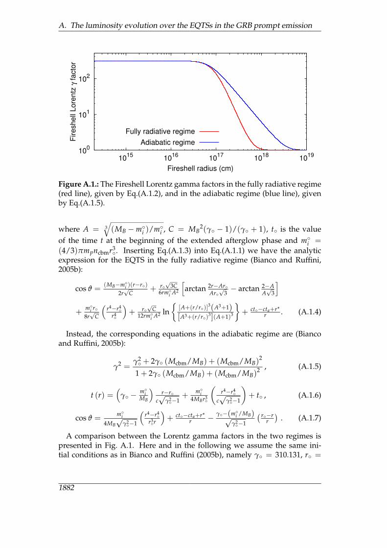
Figure A.1.: The Fireshell Lorentz gamma factors in the fully radiative regime(red line), given by Eq.(A.1.2), and in the adiabatic regime (blue line), givenby Eq.(A.1.5).
where A = 3√(MB −mi )/mi , C = MB
2(γ − 1)/(γ + 1), t is the valueof the time t at the beginning of the extended afterglow phase and mi =(4/3)πmpncbmr3
. Inserting Eq.(A.1.3) into Eq.(A.1.1) we have the analyticexpression for the EQTS in the fully radiative regime (Bianco and Ruffini,2005b):
cos ϑ =(MB−mi )(r−r)
2r√
C+ r
√3C
6rmi A2
[arctan 2r−Ar
Ar√
3− arctan 2−A
A√
3
]+
mi r8r√
C
(r4−r4
r4
)+ r
√C
12rmi A2 ln
[A+(r/r)]3(A3+1)[A3+(r/r)3](A+1)3
+ ct−cta+r?
r . (A.1.4)
Instead, the corresponding equations in the adiabatic regime are (Biancoand Ruffini, 2005b):
γ2 =γ2 + 2γ (Mcbm/MB) + (Mcbm/MB)
2
1 + 2γ (Mcbm/MB) + (Mcbm/MB)2 , (A.1.5)
t (r) =(
γ −miMB
)r−r
c√
γ2−1+
mi4MBr3
(r4−r4
c√
γ2−1
)+ t , (A.1.6)
cos ϑ =mi
4MB√
γ2−1
(r4−r4
r3r
)+ ct−cta+r?
r − γ−(mi /MB)√γ2−1
( r−rr)
. (A.1.7)
A comparison between the Lorentz gamma factors in the two regimes ispresented in Fig. A.1. Here and in the following we assume the same ini-tial conditions as in Bianco and Ruffini (2005b), namely γ = 310.131, r =
1882
A.2. The extended afterglow luminosity distribution over the EQTS
1.943× 1014 cm, t = 6.481× 10³ s, r? = 2.354× 108 cm, ncbm = 1.0 particles/cm3,MB = 1.61× 1030 g.
A.2. The extended afterglow luminositydistribution over the EQTS
Within the fireshell model, the GRB extended afterglow bolometric luminos-ity in an arrival time dta and per unit solid angle dΩ is given by (details inRuffini et al., 2009, and refs. therein):
dEγ
dtadΩ≡∫
EQTSL(r, ϑ, ϕ; ta)dΣ =
∫EQTS
∆ε cos ϑvdt4πΛ4dta
dΣ, (A.2.1)
where ∆ε is the energy density released in the interaction of the ABM pulsewith the CBM measured in the comoving frame, Λ = γ(1− (v/c) cos ϑ) isthe Doppler factor, dΣ is the surface element of the EQTS at arrival time taon which the integration is performed, and it has been assumed the fullyradiative condition. We are here not considering the cosmological redshiftof the source, which is constant during the GRB explosion and therefore itcannot affect the results of the present analysis. We recall that in our casesuch a bolometric luminosity is a good approximation of the one observedin the prompt emission and in the early afterglow by e.g. the BAT or GBMinstruments (Ruffini et al., 2002, 2004b).
We are now going to show how this luminosity is distributed over theEQTSs, i.e. we are going to plot over selected EQTSs the luminosity densityL(r, ϑ, ϕ; ta). The results are represented in Fig. A.2. We chose eight differ-ent EQTSs, corresponding to arrival time values ranging from the promptemission (5 seconds) to the early (1 hour) afterglow phases. For each EQTSwe represent also the boundaries of the visible region due to relativistic colli-mation, defined by the condition (see e.g. Bianco and Ruffini, 2006, and refs.therein):
cos ϑ ≥ v/c . (A.2.2)
We obtain that, at the beginning (ta = 5 seconds), when γ is approximatelyconstant, the most luminous regions of the EQTS are the ones along the lineof sight. However, as γ starts to drop (ta & 30 seconds), the most luminousregions of the EQTSs become the ones closest to the boundary of the visibleregion.
A.3. Conclusions
Within the fireshell model, using the exact analytic expressions for the fireshellequations of motion and for the corresponding EQTSs in the fully radiative
1883
A. The luminosity evolution over the EQTSs in the GRB prompt emission
ta = 5 seconds
0.0x100
1.0x10¹⁶
2.0x10¹⁶
3.0x10¹⁶
Distance (cm)
-4.0x10¹³
-2.0x10¹³
0.0x100
2.0x10¹³
4.0x10¹³
Dis
tance (
cm
)
1025
1026
1027
Lum
inosity d
ensity (
erg
/(s*c
m2))
ta = 10 seconds
0.0x100
2.0x10¹⁶
4.0x10¹⁶
6.0x10¹⁶
Distance (cm)
-1.0x10¹⁴
-5.0x10¹³
0.0x100
5.0x10¹³
1.0x10¹⁴
Dis
tance (
cm
)
1025
1026
1027
Lum
inosity d
ensity (
erg
/(s*c
m2))
ta = 30 seconds
0.0x100
2.0x10¹⁶
4.0x10¹⁶
6.0x10¹⁶
8.0x10¹⁶
1.0x10¹⁷
Distance (cm)
-3.0x10¹⁴
-2.0x10¹⁴
-1.0x10¹⁴
0.0x100
1.0x10¹⁴
2.0x10¹⁴
3.0x10¹⁴
Dis
tance (
cm
)
1024
1025
Lum
inosity d
ensity (
erg
/(s*c
m2))
ta = 1 minute
0.0x100
5.0x10¹⁶
1.0x10¹⁷
1.5x10¹⁷
Distance (cm)
-4.0x10¹⁴
-2.0x10¹⁴
0.0x100
2.0x10¹⁴
4.0x10¹⁴
Dis
tance (
cm
)
1022
1023
1024
Lum
inosity d
ensity (
erg
/(s*c
m2))
ta = 5 minutes
0.0x100
5.0x10¹⁶
1.0x10¹⁷
1.5x10¹⁷
2.0x10¹⁷
Distance (cm)
-1.5x10¹⁵
-1.0x10¹⁵
-5.0x10¹⁴
0.0x100
5.0x10¹⁴
1.0x10¹⁵
1.5x10¹⁵
Dis
tance (
cm
)
1020
1021
1022
Lum
inosity d
ensity (
erg
/(s*c
m2))
ta = 10 minutes
0.0x100
5.0x10¹⁶
1.0x10¹⁷
1.5x10¹⁷
2.0x10¹⁷
Distance (cm)
-2.0x10¹⁵
-1.5x10¹⁵
-1.0x10¹⁵
-5.0x10¹⁴
0.0x100
5.0x10¹⁴
1.0x10¹⁵
1.5x10¹⁵
2.0x10¹⁵
Dis
tance (
cm
)
1019
1020
1021
Lum
inosity d
ensity (
erg
/(s*c
m2))
ta = 30 minutes
0.0x100
5.0x10¹⁶
1.0x10¹⁷
1.5x10¹⁷
2.0x10¹⁷
2.5x10¹⁷
Distance (cm)
-4.0x10¹⁵
-3.0x10¹⁵
-2.0x10¹⁵
-1.0x10¹⁵
0.0x100
1.0x10¹⁵
2.0x10¹⁵
3.0x10¹⁵
4.0x10¹⁵
Dis
tance (
cm
)
1017
1018
1019
Lum
inosity d
ensity (
erg
/(s*c
m2))
ta = 1 hour
0.0x100
5.0x10¹⁶
1.0x10¹⁷
1.5x10¹⁷
2.0x10¹⁷
2.5x10¹⁷
3.0x10¹⁷
Distance (cm)
-6.0x10¹⁵
-4.0x10¹⁵
-2.0x10¹⁵
0.0x100
2.0x10¹⁵
4.0x10¹⁵
6.0x10¹⁵
Dis
tance (
cm
)
1016
1017
1018
Lum
inosity d
ensity (
erg
/(s*c
m2))
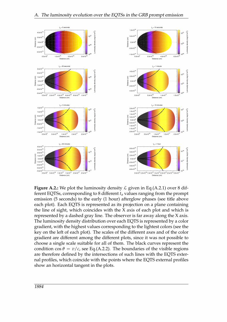
Figure A.2.: We plot the luminosity density L given in Eq.(A.2.1) over 8 dif-ferent EQTSs, corresponding to 8 different ta values ranging from the promptemission (5 seconds) to the early (1 hour) afterglow phases (see title aboveeach plot). Each EQTS is represented as its projection on a plane containingthe line of sight, which coincides with the X axis of each plot and which isrepresented by a dashed gray line. The observer is far away along the X axis.The luminosity density distribution over each EQTS is represented by a colorgradient, with the highest values corresponding to the lightest colors (see thekey on the left of each plot). The scales of the different axes and of the colorgradient are different among the different plots, since it was not possible tochoose a single scale suitable for all of them. The black curves represent thecondition cos ϑ = v/c, see Eq.(A.2.2). The boundaries of the visible regionsare therefore defined by the intersections of such lines with the EQTS exter-nal profiles, which coincide with the points where the EQTS external profilesshow an horizontal tangent in the plots.
1884
A.3. Conclusions
condition, we analyzed the temporal evolution of the distribution of the ex-tended afterglow luminosity over the EQTS during the prompt emission andthe early afterglow phases. We find that, at the beginning of the prompt emis-sion (ta = 5 seconds), when γ is approximately constant, the most luminousregions of the EQTS are the ones along the line of sight. As γ starts to drop(ta & 30 seconds), the most luminous regions of the EQTSs become the onesclosest to the boundary of the visible region. The EQTSs of GRB extendedafterglows should therefore appear in the sky as point-like sources at the be-ginning of the prompt emission but evolving after a few seconds into expand-ing luminous “rings”, with an apparent radius evolving in time and alwaysequal to the maximum transverse EQTS visible radius r⊥.
1885

B. The apparent radius of theequitemporal surfaces in the sky
From sec. A.2 we obtain that within the fireshell model the EQTSs of GRBextended afterglows should appear in the sky as point-like sources at thebeginning of the prompt emission but evolving after a few seconds into ex-panding luminous “rings”, with an apparent radius evolving in time andalways equal to the maximum transverse EQTS visible radius r⊥ which canbe obtained from Eqs.(A.1.1,A.2.2):
r⊥ = r sin ϑcta = ct (r)− r cos ϑ + r?
cos ϑ = v/c. (B.0.1)
where t = t(r) is given by Eq.(A.1.3). With a small algebra we get:r⊥ = r/γ(r)ta = t(r)− (r/c)
√1− γ(r)−2 + (r?/c)
, (B.0.2)
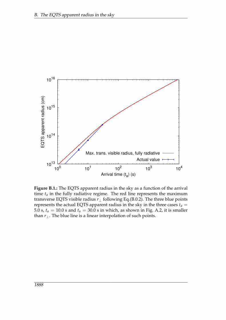
where γ ≡ γ (r) is given by Eq.(A.1.2) and t ≡ t (r) is given by Eq.(A.1.3),since we assumed the fully radiative condition. Eq.(B.0.2) defines parametri-cally the evolution of r⊥ ≡ r⊥ (ta), i.e. the evolution of the maximum trans-verse EQTS visible radius as a function of the arrival time. In Fig. A.2 wesaw that such r⊥ coincides with the actual value of the EQTS apparent ra-dius in the sky only for ta & 30 s, since for ta . 30 s the most luminousEQTS regions are the ones closest to the line of sight (see the first three plotsin Fig. A.2). Therefore, in Fig. B.1 we plot r⊥ given by Eq.(B.0.2) in the fullyradiative regime together with the actual values of the EQTS apparent radiusin the sky taken from Fig. A.2 in the three cases in which they are different.It is clear that, during the early phases of the prompt emission, even the “ex-act solution” given by Eq.(B.0.2) can be considered only an upper limit to theactual EQTS apparent radius in the sky.
In the current literature (see e.g. Sari, 1998; Waxman et al., 1998; Granotet al., 1999a,b; Garnavich et al., 2000; Granot and Loeb, 2001; Gaudi et al.,2001; Galama et al., 2003; Granot and Loeb, 2003; Taylor et al., 2004; Orenet al., 2004; Granot et al., 2005; Granot, 2008) there are no analogous treat-ments, since it is always assumed an adiabatic dynamics instead of a fully ra-diative one and only the lates afterglow phases are addressed. It is usually as-
1887
B. The EQTS apparent radius in the sky
1013
1014
1015
1016
100
101
102
103
104
EQ
TS
appare
nt ra
diu
s (
cm
)
Arrival time (ta) (s)
Max. trans. visible radius, fully radiative
Actual value
Figure B.1.: The EQTS apparent radius in the sky as a function of the arrivaltime ta in the fully radiative regime. The red line represents the maximumtransverse EQTS visible radius r⊥ following Eq.(B.0.2). The three blue pointsrepresents the actual EQTS apparent radius in the sky in the three cases ta =5.0 s, ta = 10.0 s and ta = 30.0 s in which, as shown in Fig. A.2, it is smallerthan r⊥. The blue line is a linear interpolation of such points.
1888
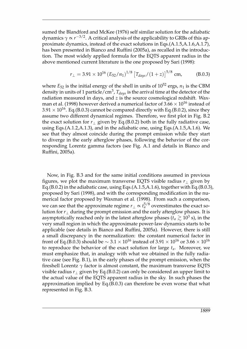
sumed the Blandford and McKee (1976) self similar solution for the adiabaticdynamics γ ∝ r−3/2. A critical analysis of the applicability to GRBs of this ap-proximate dynamics, instead of the exact solutions in Eqs.(A.1.5,A.1.6,A.1.7),has been presented in Bianco and Ruffini (2005a), as recalled in the introduc-tion. The most widely applied formula for the EQTS apparent radius in theabove mentioned current literature is the one proposed by Sari (1998):
r⊥ = 3.91× 10¹⁶ (E52/n1)1/8 [Tdays/(1 + z)
]5/8 cm, (B.0.3)
where E52 is the initial energy of the shell in units of 1052 ergs, n1 is the CBMdensity in units of 1 particle/cm3, Tdays is the arrival time at the detector of theradiation measured in days, and z is the source cosmological redshift. Wax-man et al. (1998) however derived a numerical factor of 3.66× 10¹⁶ instead of3.91× 1016. Eq.(B.0.3) cannot be compared directly with Eq.(B.0.2), since theyassume two different dynamical regimes. Therefore, we first plot in Fig. B.2the exact solution for r⊥ given by Eq.(B.0.2) both in the fully radiative case,using Eqs.(A.1.2,A.1.3), and in the adiabatic one, using Eqs.(A.1.5,A.1.6). Wesee that they almost coincide during the prompt emission while they startto diverge in the early afterglow phases, following the behavior of the cor-responding Lorentz gamma factors (see Fig. A.1 and details in Bianco andRuffini, 2005a).
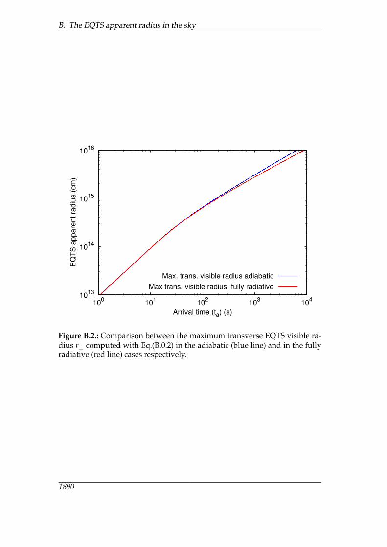
Now, in Fig. B.3 and for the same initial conditions assumed in previousfigures, we plot the maximum transverse EQTS visible radius r⊥ given byEq.(B.0.2) in the adiabatic case, using Eqs.(A.1.5,A.1.6), together with Eq.(B.0.3),proposed by Sari (1998), and with the corresponding modification in the nu-merical factor proposed by Waxman et al. (1998). From such a comparison,we can see that the approximate regime r⊥ ∝ t5/8
a overestimates the exact so-lution for r⊥ during the prompt emission and the early afterglow phases. It isasymptotically reached only in the latest afterglow phases (ta & 103 s), in thevery small region in which the approximate power-law dynamics starts to beapplicable (see details in Bianco and Ruffini, 2005a). However, there is stilla small discrepancy in the normalization: the constant numerical factor infront of Eq.(B.0.3) should be ∼ 3.1× 10¹⁶ instead of 3.91× 10¹⁶ or 3.66× 10¹⁶
to reproduce the behavior of the exact solution for large ta. Moreover, wemust emphasize that, in analogy with what we obtained in the fully radia-tive case (see Fig. B.1), in the early phases of the prompt emission, when thefireshell Lorentz γ factor is almost constant, the maximum transverse EQTSvisible radius r⊥ given by Eq.(B.0.2) can only be considered an upper limit tothe actual value of the EQTS apparent radius in the sky. In such phases theapproximation implied by Eq.(B.0.3) can therefore be even worse that whatrepresented in Fig. B.3.
1889
B. The EQTS apparent radius in the sky
1013
1014
1015
1016
100
101
102
103
104
EQ
TS
appare
nt ra
diu
s (
cm
)
Arrival time (ta) (s)
Max. trans. visible radius adiabatic
Max trans. visible radius, fully radiative
Figure B.2.: Comparison between the maximum transverse EQTS visible ra-dius r⊥ computed with Eq.(B.0.2) in the adiabatic (blue line) and in the fullyradiative (red line) cases respectively.
1890
1013
1014
1015
1016
100
101
102
103
104
EQ
TS
appare
nt ra
diu
s (
cm
)
Arrival time (ta) (s)
Max. trans. visible radius, adiabatic
Sari (1998), adiabatic
Waxman, Kulkarni, Frail (1998), adiabatic
Figure B.3.: The EQTS apparent radius in the sky as a function of the arrivaltime ta in the adiabatic regime. The red line represents the maximum trans-verse EQTS visible radius r⊥ following Eq.(B.0.2). The green line representsEq.(B.0.3) proposed by Sari (1998). The blue line represents the correspond-ing modification in the numerical factor proposed by Waxman et al. (1998).These last two lines are almost coincident on the scale of this plot.
1891
B. The EQTS apparent radius in the sky
B.1. Conclusions
We also derive an exact analytic expression for the maximum transverse EQTSvisible radius r⊥, both in the fully radiative and in the adiabatic conditions,and we compared it with the approximate formulas commonly used in thecurrent literature in the adiabatic case. We found that these last ones can notbe applied in the prompt emission nor in the early afterglow phases. Evenwhen the asymptotic regime is reached (ta & 103 s), it is necessary a cor-rection to the numerical factor in front of the expression given in Eq.(B.0.3)which should be ∼ 3.1× 10¹⁶ instead of 3.91× 10¹⁶ or 3.66× 10¹⁶.
1892
C. Exact versus approximatesolutions in Gamma-Ray Burstafterglows
The consensus has been reached that the afterglow emission originates froma relativistic thin shell of baryonic matter propagating in the CBM and that itsdescription can be obtained from the relativistic conservation laws of energyand momentum. In both our approach and in the other ones in the currentliterature (see e.g. Piran, 1999; Chiang and Dermer, 1999; Ruffini et al., 2003;Bianco and Ruffini, 2005a) such conservations laws are used. The main differ-ence is that in the current literature it is widely adopted an ultra-relativisticapproximation, following the Blandford and McKee (1976) self-similar so-lution, while we use the exact solution of the equations of motion (see theprevious report about “Gamma-Ray Bursts”). We here express such equa-tions in a differential formulation which will be most useful in comparingand contrasting our exact solutions with the ones in the current literature.
C.1. Differential formulation of the afterglowdynamics equations
We recall from the previous report about “Gamma-Ray Bursts”that the rel-ativistic conservation laws of energy and momentum lead to the followingfinite difference expression for the equations of the afterglow dynamics:
∆Eint = ρB1V1
√1 + 2γ1
∆Mcbmc2
ρB1V1+
(∆Mcbmc2
ρB1V1
)2
− ρB1V1
(1 +
∆Mcbmc2
ρB1V1
),
(C.1.1)
γ2 =γ1 +
∆Mcbmc2
ρB1 V1√1 + 2γ1
∆Mcbmc2
ρB1 V1+(
∆Mcbmc2
ρB1 V1
)2. (C.1.2)
Under the limit:∆Mcbmc2
ρB1V1 1 , (C.1.3)
1893
C. Exact vs. approximate solutions in GRB afterglows
and performing the following substitutions:
∆Eint → dEint , γ2 − γ1 → dγ , ∆Mcbm → dMcbm , (C.1.4)
Eqs.(C.1.1,C.1.2) are equivalent to:
dEint = (γ− 1) dMcbmc2 , (C.1.5a)
dγ = −γ2−1M dMcbm , (C.1.5b)
dM = 1−εc2 dEint + dMcbm , (C.1.5c)
dMcbm = 4πmpncbmr2dr , (C.1.5d)
where, we recall, Eint, γ and M are respectively the internal energy, the Lorentzfactor and the mass-energy of the expanding pulse, ncbm is the CBM num-ber density which is assumed to be constant, mp is the proton mass, ε is theemitted fraction of the energy developed in the collision with the CBM andMcbm is the amount of CBM mass swept up within the radius r: Mcbm =(4/3)π(r3 − r3)mpncbm, where r is the starting radius of the baryonic shell.
C.2. The exact analytic solutions
A first integral of these equations has been found in both our work and thecurrent literature (see e.g. Piran, 1999; Chiang and Dermer, 1999; Ruffini et al.,2003; Bianco and Ruffini, 2005a). This leads to expressions for the Lorentzgamma factor as a function of the radial coordinate. In the “fully radiativecondition” (i.e. ε = 1) we have:
γ =1 + (Mcbm/MB)
(1 + γ−1
)[1 + (1/2) (Mcbm/MB)]
γ−1 + (Mcbm/MB)
(1 + γ−1
)[1 + (1/2) (Mcbm/MB)]
, (C.2.1)
while in the “fully adiabatic condition” (i.e. ε = 0) we have:
γ2 =γ2 + 2γ (Mcbm/MB) + (Mcbm/MB)
2
1 + 2γ (Mcbm/MB) + (Mcbm/MB)2 , (C.2.2)
where γ is the initial value of the Lorentz gamma factor of the acceleratedbaryons at the beginning of the afterglow phase.
A major difference between our treatment and the ones in the current liter-ature is that we have integrated the above equations analytically. Thus we ob-tained the explicit analytic form of the equations of motion for the expandingshell in the afterglow for a constant CBM density. For the fully radiative casewe have explicitly integrated the differential equation for r (t) in Eq.(C.2.1),recalling that γ−2 = 1 − [dr/ (cdt)]2, where t is the time in the laboratory
1894
C.3. Approximations adopted in the current literature
reference frame. The new explicit analytic solution of the equations of mo-tion we have obtained for the relativistic shell in the entire range from theultra-relativistic to the non-relativistic regimes is (Bianco and Ruffini, 2005b):
t = MB−mi2c√
C(r− r) + r
√C
12cmi A2 ln
[A+(r/r)]3(A3+1)[A3+(r/r)3](A+1)3
− mi r
8c√
C
+ t +mi r8c√
C
(rr
)4+ r
√3C
6cmi A2
[arctan 2(r/r)−A
A√
3− arctan 2−A
A√
3
](C.2.3)
where we have A = 3√(
MB −mi)
/mi , C = MB2(γ− 1)/(γ+ 1) and mi =
(4/3)πmpncbmr3.
Correspondingly, in the adiabatic case we have (Bianco and Ruffini, 2005b):
t =(
γ −miMB
)r−r
c√
γ2−1+
mi4MBr3
r4−r4
c√
γ2−1+ t . (C.2.4)
C.3. Approximations adopted in the currentliterature
We turn now to the comparison of the exact solutions given in Eqs.(C.2.3)with the approximations used in the current literature. We show that such anapproximation holds only in a very limited range of the physical and astro-physical parameters and in an asymptotic regime which is reached only fora very short time, if any, and that therefore it cannot be used for modelingGRBs. Following Blandford and McKee (1976), a so-called “ultrarelativistic”approximation γ γ 1 has been widely adopted to solve Eqs.(C.1.5)(see e.g. Sari, 1997, 1998; Waxman, 1997; Rees and Meszaros, 1998; Granotet al., 1999a; Panaitescu and Meszaros, 1998; Panaitescu and Meszaros, 1999;Chiang and Dermer, 1999; Piran, 1999; Gruzinov and Waxman, 1999; vanParadijs et al., 2000; Meszaros, 2002, and references therein). This leads tosimple constant-index power-law relations:
γ ∝ r−a , (C.3.1)
with a = 3 in the fully radiative case and a = 3/2 in the fully adiabatic case.
We address now the issue of establishing the domain of applicability of thesimplified Eq.(C.3.1) used in the current literature both in the fully radiativeand adiabatic cases.
1895
C. Exact vs. approximate solutions in GRB afterglows
C.3.1. The fully radiative case
We first consider the fully radiative case. If we assume:
1/ (γ + 1) Mcbm/MB γ/ (γ + 1) < 1 , (C.3.2)
we have that in the numerator of Eq.(C.2.1) the linear term in Mcbm/MB isnegligible with respect to 1 and the quadratic term is a fortiori negligible,while in the denominator the linear term in Mcbm/MB is the leading one.Eq.(C.2.1) then becomes:
γ ' [γ/ (γ + 1)] MB/Mcbm . (C.3.3)
If we multiply the terms of Eq.(C.3.2) by (γ + 1)/γ, we obtain 1/γ (Mcbm/MB)[(γ + 1)/γ] 1, which is equivalent to:
γ [γ/(γ + 1)](MB/Mcbm) 1 , (C.3.4)
or, using Eq.(C.3.3), to:γ γ 1 , (C.3.5)
which is indeed the inequality adopted in the “ultrarelativistic” approxima-tion in the current literature. If we further assume r3 r3
, Eq.(C.3.3) can beapproximated by a simple constant-index power-law as in Eq.(C.3.1):
γ ' [γ/ (γ + 1)] MB/[(4/3)πncbmmpr3
]∝ r−3 . (C.3.6)
We turn now to the range of applicability of these approximations, consis-tently with the inequalities given in Eq.(C.3.2). It then becomes manifest thatthese inequalities can only be enforced in a finite range of Mcbm/MB. Thelower limit (LL) and the upper limit (UL) of such range can be conservativelyestimated: (
McbmMB
)LL
= 102 1γ+1 ,
(McbmMB
)UL
= 10−2 γγ+1 . (C.3.7a)
The allowed range of variability, if it exists, is then given by:(McbmMB
)UL−(
McbmMB
)LL
= 10−2 γ−104
γ+1 > 0 . (C.3.7b)
A necessary condition for the applicability of the above approximations istherefore:
γ > 104 . (C.3.8)
It is important to emphasize that Eq.(C.3.8) is only a necessary condition forthe applicability of the approximate Eq.(C.3.6) but it is not sufficient: Eq.(C.3.6)in fact can be applied only in the very limited range of r values whose upper
1896
C.3. Approximations adopted in the current literature
and lower limits are given in Eq.(C.3.7a). See for explicit examples sectionC.4 below.
C.3.2. The adiabatic case
We now turn to the adiabatic case. If we assume:
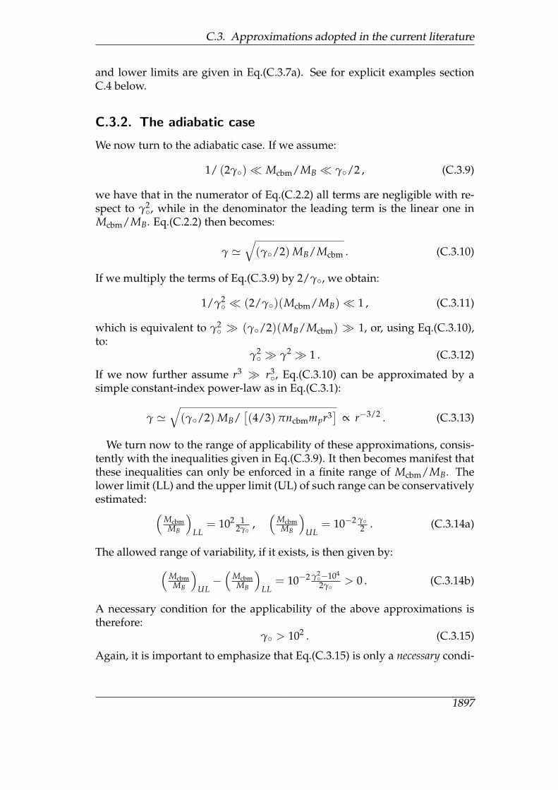
1/ (2γ) Mcbm/MB γ/2 , (C.3.9)
we have that in the numerator of Eq.(C.2.2) all terms are negligible with re-spect to γ2
, while in the denominator the leading term is the linear one inMcbm/MB. Eq.(C.2.2) then becomes:
γ '√(γ/2) MB/Mcbm . (C.3.10)
If we multiply the terms of Eq.(C.3.9) by 2/γ, we obtain:
1/γ2 (2/γ)(Mcbm/MB) 1 , (C.3.11)
which is equivalent to γ2 (γ/2)(MB/Mcbm) 1, or, using Eq.(C.3.10),
to:γ2 γ2 1 . (C.3.12)
If we now further assume r3 r3, Eq.(C.3.10) can be approximated by a
simple constant-index power-law as in Eq.(C.3.1):
γ '√(γ/2) MB/
[(4/3)πncbmmpr3
]∝ r−3/2 . (C.3.13)
We turn now to the range of applicability of these approximations, consis-tently with the inequalities given in Eq.(C.3.9). It then becomes manifest thatthese inequalities can only be enforced in a finite range of Mcbm/MB. Thelower limit (LL) and the upper limit (UL) of such range can be conservativelyestimated: (
McbmMB
)LL
= 102 12γ
,(
McbmMB
)UL
= 10−2 γ2 . (C.3.14a)
The allowed range of variability, if it exists, is then given by:(McbmMB
)UL−(
McbmMB
)LL
= 10−2 γ2−104
2γ> 0 . (C.3.14b)
A necessary condition for the applicability of the above approximations istherefore:
γ > 102 . (C.3.15)
Again, it is important to emphasize that Eq.(C.3.15) is only a necessary condi-
1897
C. Exact vs. approximate solutions in GRB afterglows
100
101
102
Lo
ren
tz γ
0
0.5
1
1.5
2
2.5
3
1014
1015
1016
1017
1018
1019
1020
1021
ae
ff
Radial coordinate (r) (cm)
a = 3.0
a = 1.5
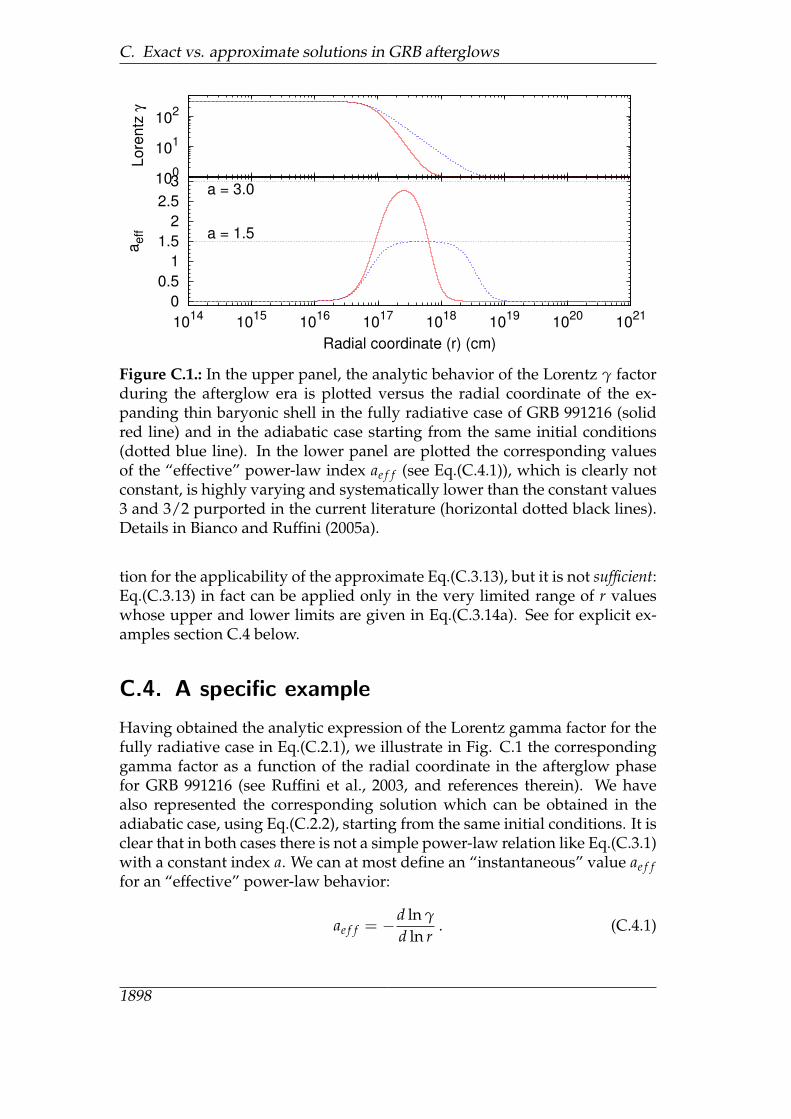
Figure C.1.: In the upper panel, the analytic behavior of the Lorentz γ factorduring the afterglow era is plotted versus the radial coordinate of the ex-panding thin baryonic shell in the fully radiative case of GRB 991216 (solidred line) and in the adiabatic case starting from the same initial conditions(dotted blue line). In the lower panel are plotted the corresponding valuesof the “effective” power-law index ae f f (see Eq.(C.4.1)), which is clearly notconstant, is highly varying and systematically lower than the constant values3 and 3/2 purported in the current literature (horizontal dotted black lines).Details in Bianco and Ruffini (2005a).
tion for the applicability of the approximate Eq.(C.3.13), but it is not sufficient:Eq.(C.3.13) in fact can be applied only in the very limited range of r valueswhose upper and lower limits are given in Eq.(C.3.14a). See for explicit ex-amples section C.4 below.
C.4. A specific example
Having obtained the analytic expression of the Lorentz gamma factor for thefully radiative case in Eq.(C.2.1), we illustrate in Fig. C.1 the correspondinggamma factor as a function of the radial coordinate in the afterglow phasefor GRB 991216 (see Ruffini et al., 2003, and references therein). We havealso represented the corresponding solution which can be obtained in theadiabatic case, using Eq.(C.2.2), starting from the same initial conditions. It isclear that in both cases there is not a simple power-law relation like Eq.(C.3.1)with a constant index a. We can at most define an “instantaneous” value ae f ffor an “effective” power-law behavior:
ae f f = −d ln γ
d ln r. (C.4.1)
1898
C.4. A specific example
100
101
102
103
Lo
ren
tz γ
0
0.5
1
1.5
2
2.5
3
1014
1015
1016
1017
1018
1019
1020
1021
ae
ff
Radial coordinate (r) (cm)
a = 3.0
a = 1.5
100
103
106
Lo
ren
tz γ
0
0.5
1
1.5
2
2.5
3
1014
1015
1016
1017
1018
1019
1020
1021
ae
ff
Radial coordinate (r) (cm)
a = 3.0
a = 1.5
100
102
104
Lo
ren
tz γ
0
0.5
1
1.5
2
2.5
3
1014
1015
1016
1017
1018
1019
1020
1021
ae
ff
Radial coordinate (r) (cm)
a = 3.0
a = 1.5
100
104
108
Lo
ren
tz γ
0
0.5
1
1.5
2
2.5
3
1014
1015
1016
1017
1018
1019
1020
1021
ae
ff
Radial coordinate (r) (cm)
a = 3.0
a = 1.5
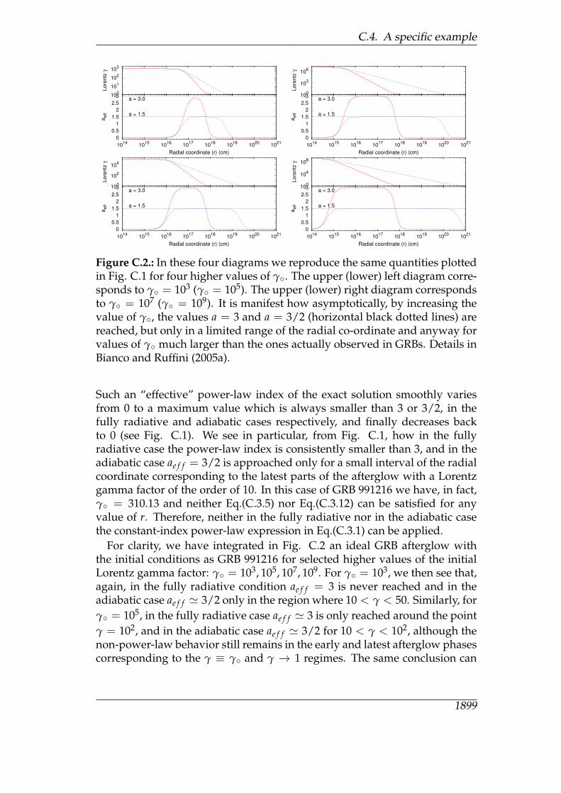
Figure C.2.: In these four diagrams we reproduce the same quantities plottedin Fig. C.1 for four higher values of γ. The upper (lower) left diagram corre-sponds to γ = 103 (γ = 105). The upper (lower) right diagram correspondsto γ = 107 (γ = 109). It is manifest how asymptotically, by increasing thevalue of γ, the values a = 3 and a = 3/2 (horizontal black dotted lines) arereached, but only in a limited range of the radial co-ordinate and anyway forvalues of γ much larger than the ones actually observed in GRBs. Details inBianco and Ruffini (2005a).
Such an “effective” power-law index of the exact solution smoothly variesfrom 0 to a maximum value which is always smaller than 3 or 3/2, in thefully radiative and adiabatic cases respectively, and finally decreases backto 0 (see Fig. C.1). We see in particular, from Fig. C.1, how in the fullyradiative case the power-law index is consistently smaller than 3, and in theadiabatic case ae f f = 3/2 is approached only for a small interval of the radialcoordinate corresponding to the latest parts of the afterglow with a Lorentzgamma factor of the order of 10. In this case of GRB 991216 we have, in fact,γ = 310.13 and neither Eq.(C.3.5) nor Eq.(C.3.12) can be satisfied for anyvalue of r. Therefore, neither in the fully radiative nor in the adiabatic casethe constant-index power-law expression in Eq.(C.3.1) can be applied.
For clarity, we have integrated in Fig. C.2 an ideal GRB afterglow withthe initial conditions as GRB 991216 for selected higher values of the initialLorentz gamma factor: γ = 103, 105, 107, 109. For γ = 103, we then see that,again, in the fully radiative condition ae f f = 3 is never reached and in theadiabatic case ae f f ' 3/2 only in the region where 10 < γ < 50. Similarly, forγ = 105, in the fully radiative case ae f f ' 3 is only reached around the pointγ = 102, and in the adiabatic case ae f f ' 3/2 for 10 < γ < 102, although thenon-power-law behavior still remains in the early and latest afterglow phasescorresponding to the γ ≡ γ and γ → 1 regimes. The same conclusion can
1899
C. Exact vs. approximate solutions in GRB afterglows
be reached for the remaining cases γ = 107 and γ = 109.We like to emphasize that the early part of the afterglow, where γ ≡ γ,
which cannot be described by the constant-index power-law approximation,do indeed corresponds to the rising part of the afterglow bolometric lumi-nosity and to its peak, which is reached as soon as the Lorentz gamma factorstarts to decrease. We have shown (see e.g. Ruffini et al., 2001a, 2003, 2005,and references therein) how the correct identifications of the raising part andthe peak of the afterglow are indeed crucial for the explanation of the ob-served “prompt radiation”. Similarly, the power-law cannot be applied dur-ing the entire approach to the newtonian regime, which corresponds to someof the actual observations occurring in the latest afterglow phases.
1900
D. Exact analytic expressions forthe equitemporal surfaces inGamma-Ray Burst afterglows
D.1. The definition of the EQTSs
For a relativistically expanding spherically symmetric source the “equitem-poral surfaces” (EQTSs, namely the locus of source points of the signals ar-riving at the observer at the same time) are surfaces of revolution about theline of sight. The general expression for their profile, in the form ϑ = ϑ(r),corresponding to an arrival time ta of the photons at the detector, can be ob-tained from (see e.g. Ruffini et al., 2003; Bianco and Ruffini, 2004, 2005b, andFigs. D.1–D.4):
cta = ct (r)− r cos ϑ + r? , (D.1.1)
where r? is the initial size of the expanding source, ϑ is the angle between theradial expansion velocity of a point on its surface and the line of sight, andt = t(r) is its equation of motion, expressed in the laboratory frame, obtainedby the integration of Eqs.(C.1.5). From the definition of the Lorentz gammafactor γ−2 = 1− (dr/cdt)2, we have in fact:
ct (r) =∫ r
0
[1− γ−2 (r′)]−1/2
dr′ , (D.1.2)
where γ(r) comes from the integration of Eqs.(C.1.5).
It is appropriate to underline a basic difference between the apparent su-perluminal velocity orthogonal to the line of sight, v⊥ ' γv, and the appar-ent superluminal velocity along the line of sight, v‖ ' γ2v. In the case ofGRBs, this last one is the most relevant: for a Lorentz gamma factor γ ' 300we have v‖ ' 105c. This is self-consistently verified in the structure of the“prompt radiation” of GRBs (see e.g. Ruffini et al., 2002).
1901
D. Exact analytic expressions for the EQTSs in GRB afterglows
-100
-50
0
50
100
10-2
10-1
100
101
102
103
104
105
106
107
108
Op
en
ing
an
gle
ϑm
ax (
de
gre
es)
Detector arrival time (tad) (s)
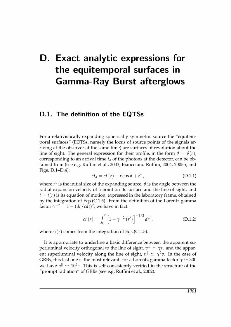
Figure D.1.: Not all values of ϑ are allowed. Only photons emitted at an anglesuch that cos ϑ ≥ (v/c) can be viewed by the observer. Thus the maximumallowed ϑ value ϑmax corresponds to cos ϑmax = (v/c). In this figure weshow ϑmax (i.e. the angular amplitude of the visible area of the ABM pulse)in degrees as a function of the arrival time at the detector for the photonsemitted along the line of sight (see text). In the earliest GRB phases v ∼ c andso ϑmax ∼ 0. On the other hand, in the latest phases of the afterglow the ABMpulse velocity decreases and ϑmax tends to the maximum possible value, i.e.90. Details in Ruffini et al. (2002, 2003).
1902
D.1. The definition of the EQTSs
1012
1013
1014
1015
1016
1017
1018
1019
1014
1015
1016
1017
1018
1019
AB
M p
uls
e v
isib
le a
rea
dia
me
ter
(cm
)
ABM pulse radius (r) (cm)
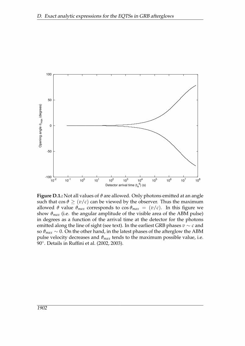
Figure D.2.: The diameter of the visible area is represented as a function ofthe ABM pulse radius. In the earliest expansion phases (γ ∼ 310) ϑmax is verysmall (see Fig. D.3), so the visible area is just a small fraction of the total ABMpulse surface. On the other hand, in the final expansion phases ϑmax → 90
and almost all the ABM pulse surface becomes visible. Details in Ruffini et al.(2002, 2003).
1903
D. Exact analytic expressions for the EQTSs in GRB afterglows
0
5.0×10¹⁷
1.0×10¹⁸
1.5×10¹⁸
0
5.0×10¹⁷
1.0×10¹⁸
1.5×10¹⁸
0 5.0×10¹⁷
1.0×10¹⁸
1.5×10¹⁸
Dis
tance fro
m the E
MB
H (
cm
)
Distance from the EMBH (cm)
Line of sight
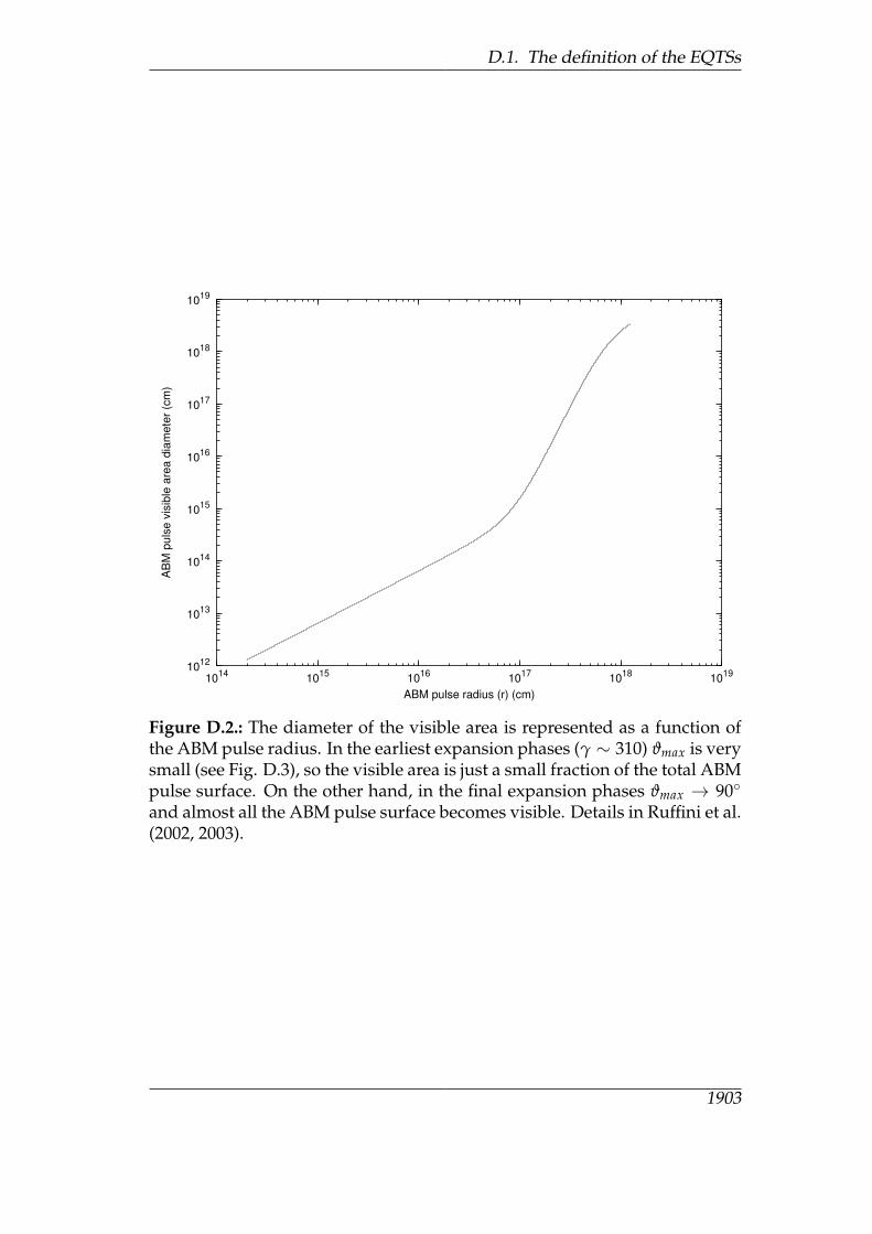
Figure D.3.: This figure shows the temporal evolution of the visible area ofthe ABM pulse. The green half-circles are the expanding ABM pulse at radiicorresponding to different laboratory times. The red curve marks the bound-ary of the visible region. The black hole is located at position (0,0) in thisplot. Again, in the earliest GRB phases the visible region is squeezed alongthe line of sight, while in the final part of the afterglow phase almost all theemitted photons reach the observer. This time evolution of the visible area iscrucial to the explanation of the GRB temporal structure. Details in Ruffiniet al. (2002, 2003).
1904
D.1. The definition of the EQTSs
3.0×10¹⁴
2.0×10¹⁴
1.0×10¹⁴
0
1.0×10¹⁴
2.0×10¹⁴
3.0×10¹⁴
0 2.0×10¹⁶
4.0×10¹⁶
6.0×10¹⁶
8.0×10¹⁶
1.0×10¹⁷
Dis
tan
ce
fro
m t
he
EM
BH
(cm
)
Distance from the EMBH (cm)
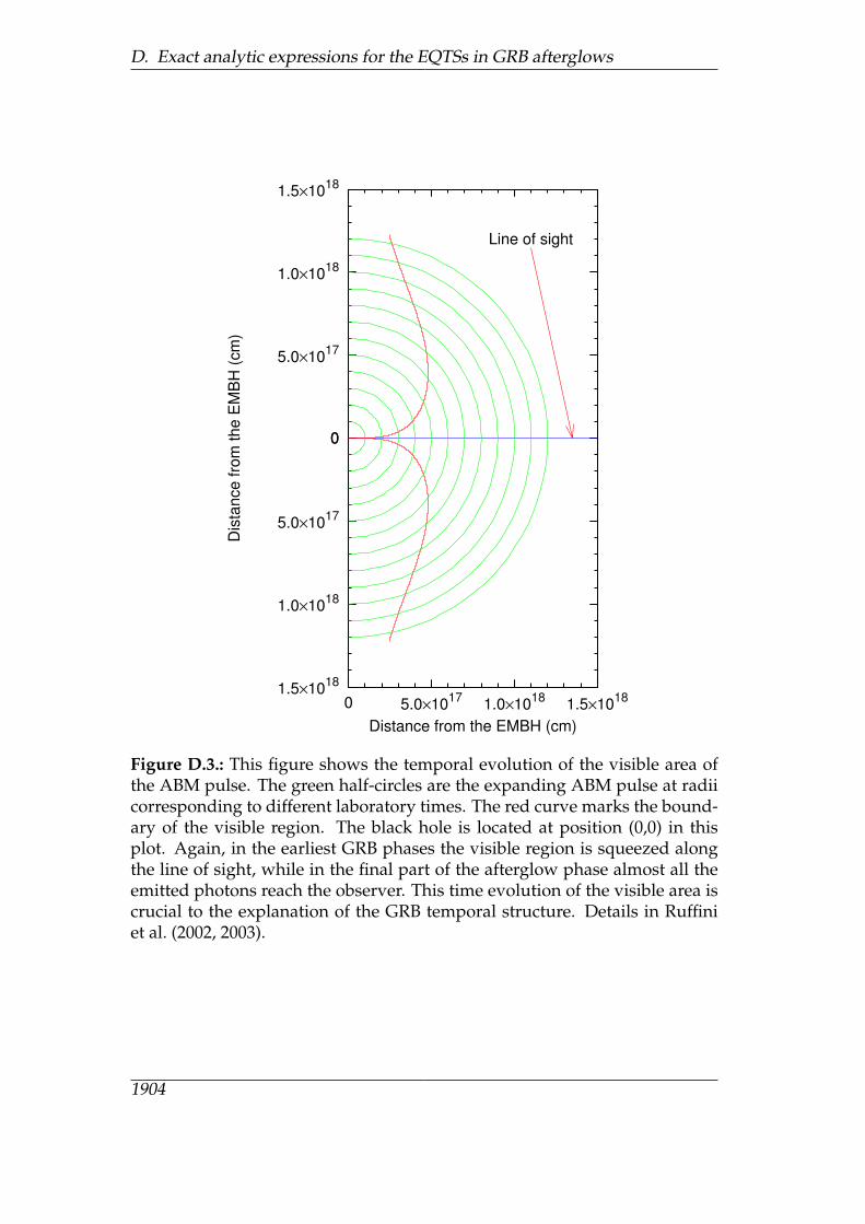
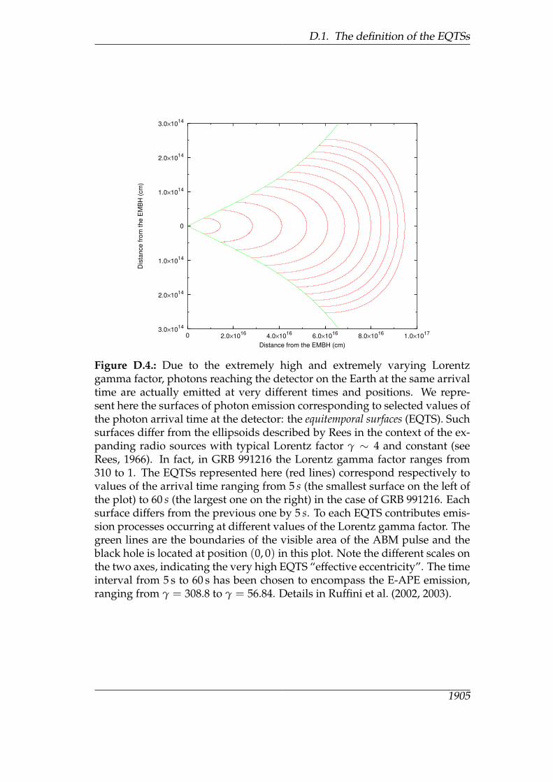
Figure D.4.: Due to the extremely high and extremely varying Lorentzgamma factor, photons reaching the detector on the Earth at the same arrivaltime are actually emitted at very different times and positions. We repre-sent here the surfaces of photon emission corresponding to selected values ofthe photon arrival time at the detector: the equitemporal surfaces (EQTS). Suchsurfaces differ from the ellipsoids described by Rees in the context of the ex-panding radio sources with typical Lorentz factor γ ∼ 4 and constant (seeRees, 1966). In fact, in GRB 991216 the Lorentz gamma factor ranges from310 to 1. The EQTSs represented here (red lines) correspond respectively tovalues of the arrival time ranging from 5 s (the smallest surface on the left ofthe plot) to 60 s (the largest one on the right) in the case of GRB 991216. Eachsurface differs from the previous one by 5 s. To each EQTS contributes emis-sion processes occurring at different values of the Lorentz gamma factor. Thegreen lines are the boundaries of the visible area of the ABM pulse and theblack hole is located at position (0, 0) in this plot. Note the different scales onthe two axes, indicating the very high EQTS “effective eccentricity”. The timeinterval from 5 s to 60 s has been chosen to encompass the E-APE emission,ranging from γ = 308.8 to γ = 56.84. Details in Ruffini et al. (2002, 2003).
1905
D. Exact analytic expressions for the EQTSs in GRB afterglows
D.2. The analytic expressions for the EQTSes
D.2.1. The fully radiative case
The analytic expression for the EQTS in the fully radiative regime can thenbe obtained substituting t(r) from Eq.(C.2.3) in Eq.(D.1.1) (see Bianco andRuffini, 2005b). We obtain:
cos ϑ =MB −mi
2r√
C(r− r) +
mi r8r√
C
[(rr
)4
− 1
]
+r√
C12rmi A2 ln
[A + (r/r)]3 (A3 + 1
)[A3 + (r/r)
3](A + 1)3
+ctr− cta
r
+r?
r+
r√
3C6rmi A2
[arctan
2 (r/r)− AA√
3− arctan
2− AA√
3
], (D.2.1)
where A, C and mi are the same as in Eq.(C.2.3).
D.2.2. The adiabatic case
The analytic expression for the EQTS in the adiabatic regime can then be ob-tained substituting t(r) from Eq.(C.2.4) in Eq.(D.1.1) (see Bianco and Ruffini,2005b). We obtain:
cos ϑ =mi
4MB√
γ2 − 1
[(rr
)3
− rr
]+
ctr
− cta
r+
r?
r−
γ −(mi /MB
)√γ2 − 1
[rr− 1]
. (D.2.2)
D.2.3. Comparison between the two cases
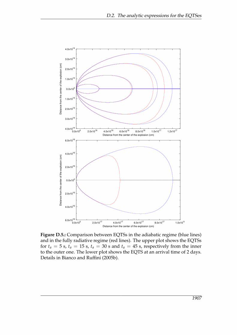
The two EQTSs are represented at selected values of the arrival time ta inFig. D.5, where the illustrative case of GRB 991216 has been used as a proto-type. The initial conditions at the beginning of the afterglow era are in thiscase given by γ = 310, r = 1.94× 1014 cm, t = 6.48× 10³ s, r? = 2.35× 10⁸
cm (see Ruffini et al., 2001b,a, 2002, 2003; Bianco and Ruffini, 2005b).
1906
D.2. The analytic expressions for the EQTSes
4.0x10¹⁴
3.0x10¹⁴
2.0x10¹⁴
1.0x10¹⁴
0.0x100
1.0x10¹⁴
2.0x10¹⁴
3.0x10¹⁴
4.0x10¹⁴
0.0x100
2.0x10¹⁶
4.0x10¹⁶
6.0x10¹⁶
8.0x10¹⁶
1.0x10¹⁷
1.2x10¹⁷
Dis
tance fro
m the c
ente
r of th
e e
xplo
sio
n (
cm
)
Distance from the center of the explosion (cm)
6.0x10¹⁶
4.0x10¹⁶
2.0x10¹⁶
0.0x100
2.0x10¹⁶
4.0x10¹⁶
6.0x10¹⁶
0.0x100
2.0x10¹⁷
4.0x10¹⁷
6.0x10¹⁷
8.0x10¹⁷
1.0x10¹⁸
Dis
tance fro
m the c
ente
r of th
e e
xplo
sio
n (
cm
)
Distance from the center of the explosion (cm)
Figure D.5.: Comparison between EQTSs in the adiabatic regime (blue lines)and in the fully radiative regime (red lines). The upper plot shows the EQTSsfor ta = 5 s, ta = 15 s, ta = 30 s and ta = 45 s, respectively from the innerto the outer one. The lower plot shows the EQTS at an arrival time of 2 days.Details in Bianco and Ruffini (2005b).
1907
D. Exact analytic expressions for the EQTSs in GRB afterglows
D.3. Approximations adopted in the currentliterature
In the current literature two different treatments of the EQTSs exist: one byPanaitescu and Meszaros (1998) and one by Sari (1998) later applied also byGranot et al. (1999a) (see also Piran, 1999, 2000; van Paradijs et al., 2000, andreferences therein).
In both these treatments, instead of the more precise dynamical equationsgiven in Eqs.(C.2.2,C.2.1), the simplified formula, based on the “ultrarela-tivistic” approximation, given in Eq.(C.3.1) has been used. A critical analysiscomparing and contrasting our exact solutions with Eq.(C.3.1) has been pre-sented in the previous section and in Bianco and Ruffini (2005a). As a furtherapproximation, instead of the exact Eq.(D.1.2), they both use the followingexpansion at first order in γ−2:
ct (r) =∫ r
0
[1 +
12γ2 (r′)
]dr′ . (D.3.1)
Correspondingly, instead of the exact Eq.(C.2.4) and Eq.(C.2.3), they find:
t (r) =rc
[1 +
12 (2a + 1) γ2 (r)
], (D.3.2a)
t (r) =rc
[1 +
116γ2 (r)
]. (D.3.2b)
The first expression has been given by Panaitescu and Meszaros (1998) andapplies both in the adiabatic (a = 3/2) and in the fully radiative (a = 3)cases (see their Eq.(2)). The second one has been given by Sari (1998) in theadiabatic case (see his Eq.(2)). Note that the first expression, in the case a =3/2, does not coincide with the second one: Sari (1998) uses a Lorentz gammafactor Γ of a shock front propagating in the expanding pulse, with Γ =
√2γ.
Instead of the exact Eqs.(D.1.1), Panaitescu and Meszaros (1998) and Sari(1998) both uses the following equation:
cta = ct (r)− r cos ϑ , (D.3.3)
where the initial size r? has been neglected. The following approximate ex-
1908
D.3. Approximations adopted in the current literature
pressions for the EQTSs have been then presented:
ϑ = 2 arcsin
12γ
√2γ2cta
r− 1
2a + 1
(rr
)2a , (D.3.4a)
cos ϑ = 1− 116γ2
L
[(rrL
)−1
−(
rrL
)3]
. (D.3.4b)
The first expression has been given by Panaitescu and Meszaros (1998) andapplies both in the adiabatic (a = 3/2) and in the fully radiative (a = 3) cases(see their Eq.(3)). The second expression, where γL ≡ γ(ϑ = 0) over thegiven EQTS and rL = 16γ2
Lcta, has been given by Sari (1998) in the adiabaticcase (see his Eq.(5)).
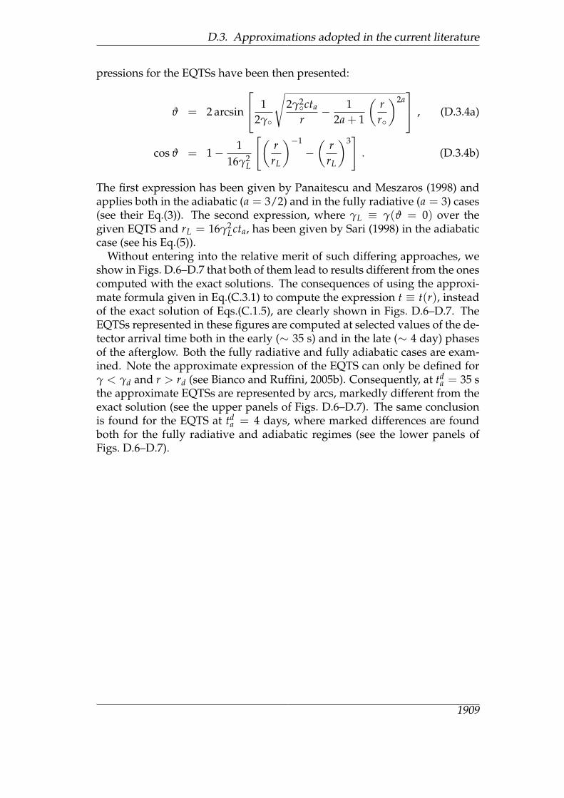
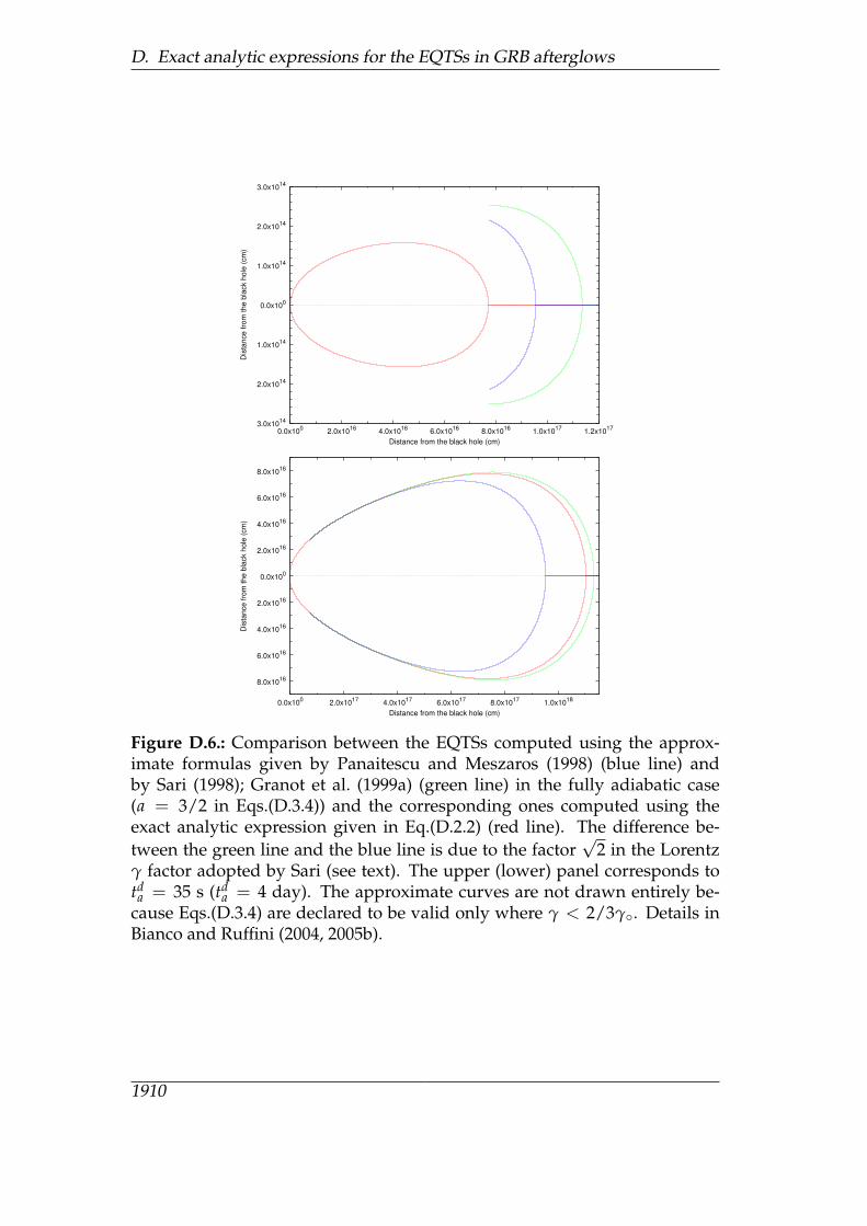
Without entering into the relative merit of such differing approaches, weshow in Figs. D.6–D.7 that both of them lead to results different from the onescomputed with the exact solutions. The consequences of using the approxi-mate formula given in Eq.(C.3.1) to compute the expression t ≡ t(r), insteadof the exact solution of Eqs.(C.1.5), are clearly shown in Figs. D.6–D.7. TheEQTSs represented in these figures are computed at selected values of the de-tector arrival time both in the early (∼ 35 s) and in the late (∼ 4 day) phasesof the afterglow. Both the fully radiative and fully adiabatic cases are exam-ined. Note the approximate expression of the EQTS can only be defined forγ < γd and r > rd (see Bianco and Ruffini, 2005b). Consequently, at td
a = 35 sthe approximate EQTSs are represented by arcs, markedly different from theexact solution (see the upper panels of Figs. D.6–D.7). The same conclusionis found for the EQTS at td
a = 4 days, where marked differences are foundboth for the fully radiative and adiabatic regimes (see the lower panels ofFigs. D.6–D.7).
1909
D. Exact analytic expressions for the EQTSs in GRB afterglows
3.0x10¹⁴
2.0x10¹⁴
1.0x10¹⁴
0.0x100
1.0x10¹⁴
2.0x10¹⁴
3.0x10¹⁴
0.0x100
2.0x10¹⁶
4.0x10¹⁶
6.0x10¹⁶
8.0x10¹⁶
1.0x10¹⁷
1.2x10¹⁷
Dis
tance fro
m the b
lack h
ole
(cm
)
Distance from the black hole (cm)
8.0x10¹⁶
6.0x10¹⁶
4.0x10¹⁶
2.0x10¹⁶
0.0x100
2.0x10¹⁶
4.0x10¹⁶
6.0x10¹⁶
8.0x10¹⁶
0.0x100
2.0x10¹⁷
4.0x10¹⁷
6.0x10¹⁷
8.0x10¹⁷
1.0x10¹⁸
Dis
tance fro
m the b
lack h
ole
(cm
)
Distance from the black hole (cm)
Figure D.6.: Comparison between the EQTSs computed using the approx-imate formulas given by Panaitescu and Meszaros (1998) (blue line) andby Sari (1998); Granot et al. (1999a) (green line) in the fully adiabatic case(a = 3/2 in Eqs.(D.3.4)) and the corresponding ones computed using theexact analytic expression given in Eq.(D.2.2) (red line). The difference be-tween the green line and the blue line is due to the factor
√2 in the Lorentz
γ factor adopted by Sari (see text). The upper (lower) panel corresponds totda = 35 s (td
a = 4 day). The approximate curves are not drawn entirely be-cause Eqs.(D.3.4) are declared to be valid only where γ < 2/3γ. Details inBianco and Ruffini (2004, 2005b).
1910
D.3. Approximations adopted in the current literature
3.0x10¹⁴
2.0x10¹⁴
1.0x10¹⁴
0.0x100
1.0x10¹⁴
2.0x10¹⁴
3.0x10¹⁴
0.0x100
1.0x10¹⁶
2.0x10¹⁶
3.0x10¹⁶
4.0x10¹⁶
5.0x10¹⁶
6.0x10¹⁶
7.0x10¹⁶
8.0x10¹⁶
9.0x10¹⁶
Dis
tan
ce
fro
m t
he
bla
ck h
ole
(cm
)
Distance from the black hole (cm)
6.0x10¹⁶
4.0x10¹⁶
2.0x10¹⁶
0.0x100
2.0x10¹⁶
4.0x10¹⁶
6.0x10¹⁶
0.0x100
1.0x10¹⁷
2.0x10¹⁷
3.0x10¹⁷
4.0x10¹⁷
5.0x10¹⁷
Dis
tan
ce
fro
m t
he
bla
ck h
ole
(cm
)
Distance from the black hole (cm)
Figure D.7.: Comparison between the EQTSs computed using the approx-imate formulas given by Panaitescu and Meszaros (1998) (blue line) in thefully radiative case (a = 3 in the first of Eqs.(D.3.4)) and the correspondingones computed using the exact analytic expression given in Eq.(D.2.1) (redline). The upper (lower) panel corresponds to td
a = 35 s (tda = 4 day). Details
in Bianco and Ruffini (2004, 2005b).
1911

E. Exact versus approximatebeaming formulas inGamma-Ray Burst afterglows
Using the exact solutions introduced in the previous sections, we here in-troduce the exact analytic expressions of the relations between the detectorarrival time td
a of the GRB afterglow radiation and the corresponding half-opening angle ϑ of the expanding source visible area due to the relativisticbeaming (see e.g. Ruffini et al., 2003). Such visible area must be computednot over the spherical surface of the shell, but over the EQuiTemporal Sur-face (EQTS) of detector arrival time td
a , i.e. over the surface locus of pointswhich are source of the radiation reaching the observer at the same arrivaltime td
a (see Bianco and Ruffini, 2004, 2005b, for details). The exact analyticexpressions for the EQTSs in GRB afterglows, which have been presented inEqs.(D.2.2)–(D.2.1) and in Bianco and Ruffini (2005b), are therefore crucial inour present derivation. This approach clearly differs from the ones in thecurrent literature, which usually neglect the contributions of the radiationemitted from the entire EQTS.
The analytic relations between tda and ϑ presented in this section allow to
compute, assuming that the expanding shell is not spherically symmetric butis confined into a narrow jet with half-opening angle ϑ, the value (td
a)jet ofthe detector arrival time at which we start to “see” the sides of the jet. A cor-responding “break” in the observed light curve should occur later than (td
a)jet
(seee.g. Sari et al., 1999). In the current literature, (tda)jet is usually defined as
the detector arrival time at which γ ∼ 1/ϑ, where γ is the Lorentz factor ofthe expanding shell (see e.g. Sari et al., 1999, and also our Eq.(E.1.2) below).In our formulation we do not consider effects of lateral spreadings of the jet.
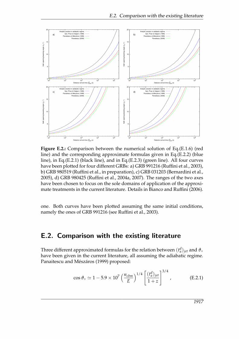
In the current literature, in the case of adiabatic regime, different approxi-mate power-law relations between (td
a)jet and ϑ have been presented, in con-trast to each other (see e.g. Sari et al., 1999; Panaitescu and Meszaros, 1999;Panaitescu, 2006). We show here that in four specific cases of GRBs, encom-passing more than 5 orders of magnitude in energy and more than 2 orders ofmagnitude in CBM density, both the one by Panaitescu and Meszaros (1999)and the one by Sari et al. (1999) overestimate the exact analytic result. A thirdrelation just presented by Panaitescu (2006) slightly underestimate the exactanalytic result. We also present an empirical fit of the numerical solutions
1913
E. Exact vs. approximate beaming formulas in GRB afterglows
of the exact equations for the adiabatic regime, compared and contrastedwith the three above approximate relations. In the fully radiative regime,and therefore in the general case, no simple power-law relation of the kindfound in the adiabatic regime can be established and the general approachwe have outlined has to be followed.
Although evidence for spherically symmetric emission in GRBs is emerg-ing from observations (Sakamoto et al., 2006) and from theoretical argumen-tations (Ruffini et al., 2004b, 2006), it is appropriate to develop here an exacttheoretical treatment of the relation between (td
a)jet and ϑ. This will allow tomake an assessment on the existence and, in the positive case, on the extentof beaming in GRBs, which in turn is going to be essential for establishingtheir correct energetics.
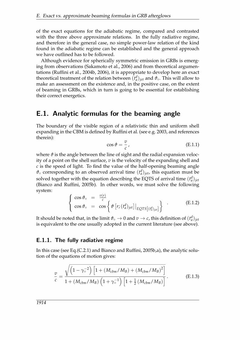
E.1. Analytic formulas for the beaming angle
The boundary of the visible region of a relativistic thin and uniform shellexpanding in the CBM is defined by Ruffini et al. (see e.g. 2003, and referencestherein):
cos ϑ =vc
, (E.1.1)
where ϑ is the angle between the line of sight and the radial expansion veloc-ity of a point on the shell surface, v is the velocity of the expanding shell andc is the speed of light. To find the value of the half-opening beaming angleϑ corresponding to an observed arrival time (td
a)jet, this equation must besolved together with the equation describing the EQTS of arrival time (td
a)jet(Bianco and Ruffini, 2005b). In other words, we must solve the followingsystem: cos ϑ = v(r)
c
cos ϑ = cos
ϑ[r; (td
a)jet]∣∣
EQTS[(tda)jet]
. (E.1.2)
It should be noted that, in the limit ϑ → 0 and v→ c, this definition of (tda)jet
is equivalent to the one usually adopted in the current literature (see above).
E.1.1. The fully radiative regime
In this case (see Eq.(C.2.1) and Bianco and Ruffini, 2005b,a), the analytic solu-tion of the equations of motion gives:
vc=
√(1− γ−2
) [
1 + (Mcbm/MB) + (Mcbm/MB)2]
1 + (Mcbm/MB)(
1 + γ−1) [
1 + 12 (Mcbm/MB)
] . (E.1.3)
1914
E.1. Analytic formulas for the beaming angle
Using the analytic expression for the EQTS given in Bianco and Ruffini (2005b)and in Eq.(D.2.1), Eq.(E.1.2) takes the form (Bianco and Ruffini, 2006):
cos ϑ =
√(1−γ−2
)[1+(Mcbm/MB)+(Mcbm/MB)2]
1+(Mcbm/MB)(1+γ−1 )
[1+ 1
2 (Mcbm/MB)]
cos ϑ =MB−mi
2r√
C(r− r) +
mi r8r√
C
[(rr
)4− 1]
+ r√
C12rmi A2 ln
[A+(r/r)]3(A3+1)[A3+(r/r)3](A+1)3
+ ct
r −c(td
a)jetr(1+z) +
r?r
+ r√
3C6rmi A2
[arctan 2(r/r)−A
A√
3− arctan 2−A
A√
3
](E.1.4)
where t is the value of the time t at the beginning of the afterglow phase,mi = (4/3)πmpncbmr3
, r? is the initial size of the expanding source, A =
[(MB − mi )/mi ]1/3, C = MB
2(γ − 1)/(γ + 1) and z is the cosmologicalredshift of the source.
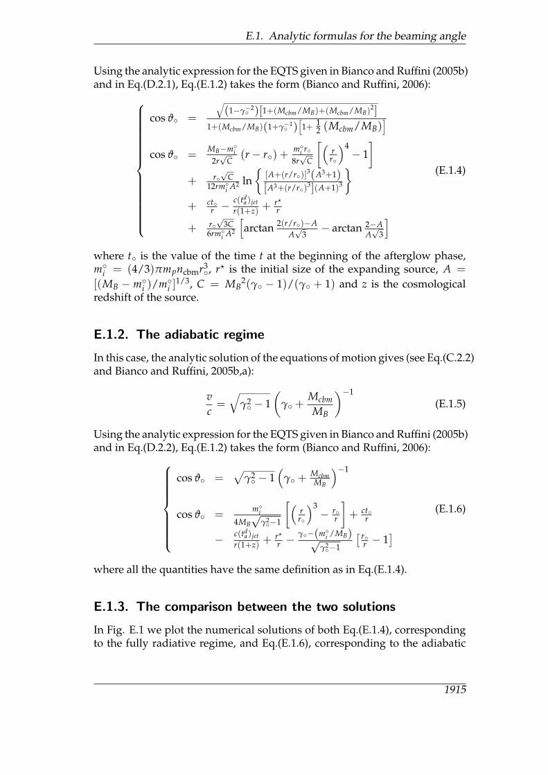
E.1.2. The adiabatic regime
In this case, the analytic solution of the equations of motion gives (see Eq.(C.2.2)and Bianco and Ruffini, 2005b,a):
vc=√
γ2 − 1
(γ +
McbmMB
)−1
(E.1.5)
Using the analytic expression for the EQTS given in Bianco and Ruffini (2005b)and in Eq.(D.2.2), Eq.(E.1.2) takes the form (Bianco and Ruffini, 2006):
cos ϑ =√
γ2 − 1
(γ +
McbmMB
)−1
cos ϑ =mi
4MB√
γ2−1
[(rr
)3− r
r
]+ ct
r
− c(tda)jet
r(1+z) +r?r −
γ−(mi /MB)√γ2−1
[ rr − 1
](E.1.6)
where all the quantities have the same definition as in Eq.(E.1.4).
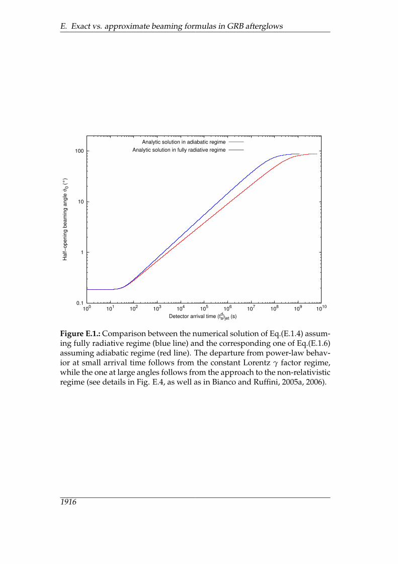
E.1.3. The comparison between the two solutions
In Fig. E.1 we plot the numerical solutions of both Eq.(E.1.4), correspondingto the fully radiative regime, and Eq.(E.1.6), corresponding to the adiabatic
1915
E. Exact vs. approximate beaming formulas in GRB afterglows
0.1
1
10
100
100
101
102
103
104
105
106
107
108
109
1010
Ha
lf−
op
en
ing
be
am
ing
an
gle
ϑ0 (
°)
Detector arrival time (tad)jet (s)
Analytic solution in adiabatic regime
Analytic solution in fully radiative regime
Figure E.1.: Comparison between the numerical solution of Eq.(E.1.4) assum-ing fully radiative regime (blue line) and the corresponding one of Eq.(E.1.6)assuming adiabatic regime (red line). The departure from power-law behav-ior at small arrival time follows from the constant Lorentz γ factor regime,while the one at large angles follows from the approach to the non-relativisticregime (see details in Fig. E.4, as well as in Bianco and Ruffini, 2005a, 2006).
1916
E.2. Comparison with the existing literature
0
5
10
15
20
102
103
104
105
106
Half−
openin
g b
eam
ing a
ngle
ϑ0 (
°)
Detector arrival time (tad)jet (s)
a)
Analytic solution in adiabatic regime
Sari, Piran & Halpern (1999)
Panaitescu & Mészáros (1999)
Panaitescu (2006)
0
5
10
15
20
102
103
104
105
106
Half−
openin
g b
eam
ing a
ngle
ϑ0 (
°)
Detector arrival time (tad)jet (s)
b)
Analytic solution in adiabatic regime
Sari, Piran & Halpern (1999)
Panaitescu & Mészáros (1999)
Panaitescu (2006)
0
5
10
15
20
102
103
104
105
106
Half−
openin
g b
eam
ing a
ngle
ϑ0 (
°)
Detector arrival time (tad)jet (s)
c)
Analytic solution in adiabatic regime
Sari, Piran & Halpern (1999)
Panaitescu & Mészáros (1999)
Panaitescu (2006)
0
5
10
15
20
102
103
104
105
106
Half−
openin
g b
eam
ing a
ngle
ϑ0 (
°)
Detector arrival time (tad)jet (s)
d)
Analytic solution in adiabatic regime
Sari, Piran & Halpern (1999)
Panaitescu & Mészáros (1999)
Panaitescu (2006)
Figure E.2.: Comparison between the numerical solution of Eq.(E.1.6) (redline) and the corresponding approximate formulas given in Eq.(E.2.2) (blueline), in Eq.(E.2.1) (black line), and in Eq.(E.2.3) (green line). All four curveshave been plotted for four different GRBs: a) GRB 991216 (Ruffini et al., 2003),b) GRB 980519 (Ruffini et al., in preparation), c) GRB 031203 (Bernardini et al.,2005), d) GRB 980425 (Ruffini et al., 2004a, 2007). The ranges of the two axeshave been chosen to focus on the sole domains of application of the approxi-mate treatments in the current literature. Details in Bianco and Ruffini (2006).
one. Both curves have been plotted assuming the same initial conditions,namely the ones of GRB 991216 (see Ruffini et al., 2003).
E.2. Comparison with the existing literature
Three different approximated formulas for the relation between (tda)jet and ϑ
have been given in the current literature, all assuming the adiabatic regime.Panaitescu and Meszaros (1999) proposed:
cos ϑ ' 1− 5.9× 10⁷(ncbm
E
)1/4[(td
a)jet
1 + z
]3/4
, (E.2.1)
1917
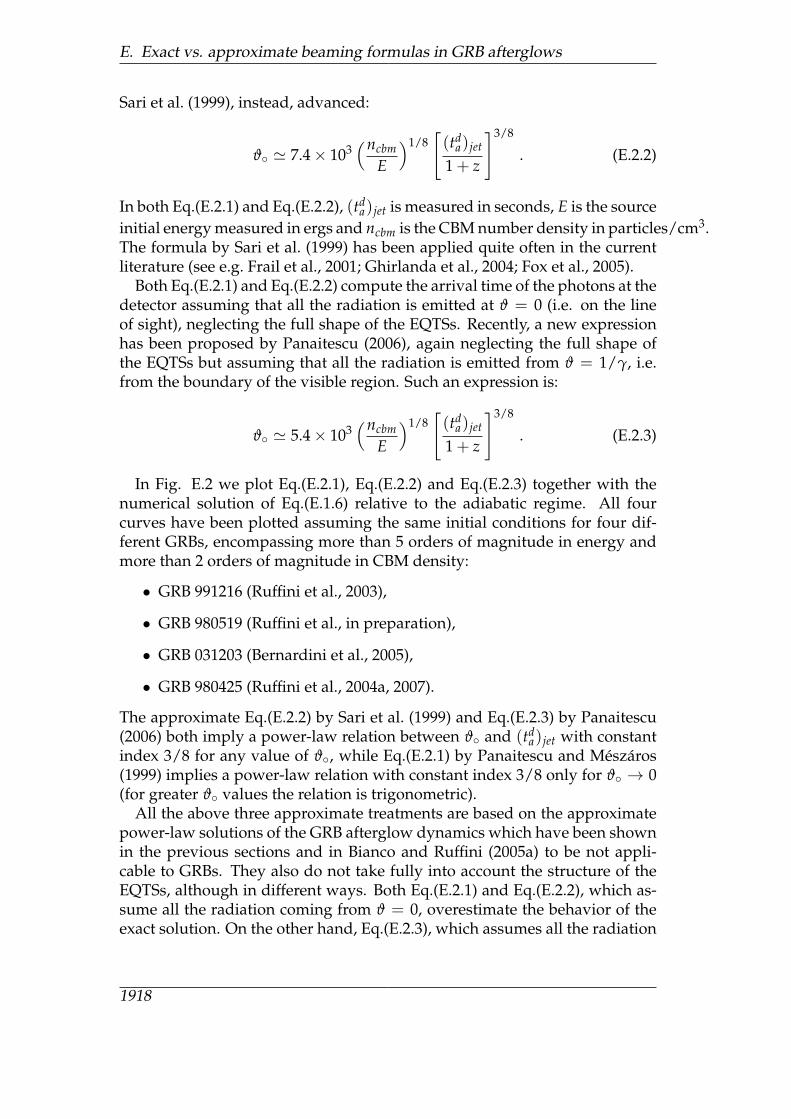
E. Exact vs. approximate beaming formulas in GRB afterglows
Sari et al. (1999), instead, advanced:
ϑ ' 7.4× 10³(ncbm
E
)1/8[(td
a)jet
1 + z
]3/8
. (E.2.2)
In both Eq.(E.2.1) and Eq.(E.2.2), (tda)jet is measured in seconds, E is the source
initial energy measured in ergs and ncbm is the CBM number density in particles/cm3.The formula by Sari et al. (1999) has been applied quite often in the currentliterature (see e.g. Frail et al., 2001; Ghirlanda et al., 2004; Fox et al., 2005).
Both Eq.(E.2.1) and Eq.(E.2.2) compute the arrival time of the photons at thedetector assuming that all the radiation is emitted at ϑ = 0 (i.e. on the lineof sight), neglecting the full shape of the EQTSs. Recently, a new expressionhas been proposed by Panaitescu (2006), again neglecting the full shape ofthe EQTSs but assuming that all the radiation is emitted from ϑ = 1/γ, i.e.from the boundary of the visible region. Such an expression is:
ϑ ' 5.4× 10³(ncbm
E
)1/8[(td
a)jet
1 + z
]3/8
. (E.2.3)
In Fig. E.2 we plot Eq.(E.2.1), Eq.(E.2.2) and Eq.(E.2.3) together with thenumerical solution of Eq.(E.1.6) relative to the adiabatic regime. All fourcurves have been plotted assuming the same initial conditions for four dif-ferent GRBs, encompassing more than 5 orders of magnitude in energy andmore than 2 orders of magnitude in CBM density:
• GRB 991216 (Ruffini et al., 2003),
• GRB 980519 (Ruffini et al., in preparation),
• GRB 031203 (Bernardini et al., 2005),
• GRB 980425 (Ruffini et al., 2004a, 2007).
The approximate Eq.(E.2.2) by Sari et al. (1999) and Eq.(E.2.3) by Panaitescu(2006) both imply a power-law relation between ϑ and (td
a)jet with constantindex 3/8 for any value of ϑ, while Eq.(E.2.1) by Panaitescu and Meszaros(1999) implies a power-law relation with constant index 3/8 only for ϑ → 0(for greater ϑ values the relation is trigonometric).
All the above three approximate treatments are based on the approximatepower-law solutions of the GRB afterglow dynamics which have been shownin the previous sections and in Bianco and Ruffini (2005a) to be not appli-cable to GRBs. They also do not take fully into account the structure of theEQTSs, although in different ways. Both Eq.(E.2.1) and Eq.(E.2.2), which as-sume all the radiation coming from ϑ = 0, overestimate the behavior of theexact solution. On the other hand, Eq.(E.2.3), which assumes all the radiation
1918
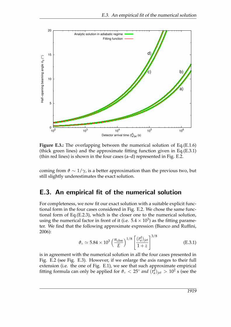
E.3. An empirical fit of the numerical solution
0
5
10
15
20
102
103
104
105
106
Ha
lf−
op
en
ing
be
am
ing
an
gle
ϑ0 (
°)
Detector arrival time (tad)jet (s)
a)
c) b)
d)
Analytic solution in adiabatic regime
Fitting function
Figure E.3.: The overlapping between the numerical solution of Eq.(E.1.6)(thick green lines) and the approximate fitting function given in Eq.(E.3.1)(thin red lines) is shown in the four cases (a–d) represented in Fig. E.2.
coming from ϑ ∼ 1/γ, is a better approximation than the previous two, butstill slightly underestimates the exact solution.
E.3. An empirical fit of the numerical solution
For completeness, we now fit our exact solution with a suitable explicit func-tional form in the four cases considered in Fig. E.2. We chose the same func-tional form of Eq.(E.2.3), which is the closer one to the numerical solution,using the numerical factor in front of it (i.e. 5.4× 10³) as the fitting parame-ter. We find that the following approximate expression (Bianco and Ruffini,2006):
ϑ ' 5.84× 10³(ncbm
E
)1/8[(td
a)jet
1 + z
]3/8
(E.3.1)
is in agreement with the numerical solution in all the four cases presented inFig. E.2 (see Fig. E.3). However, if we enlarge the axis ranges to their fullextension (i.e. the one of Fig. E.1), we see that such approximate empiricalfitting formula can only be applied for ϑ < 25 and (td
a)jet > 102 s (see the
1919
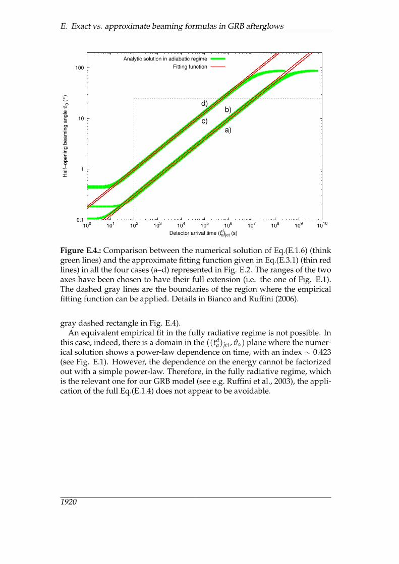
E. Exact vs. approximate beaming formulas in GRB afterglows
0.1
1
10
100
100
101
102
103
104
105
106
107
108
109
1010
Ha
lf−
op
en
ing
be
am
ing
an
gle
ϑ0 (
°)
Detector arrival time (tad)jet (s)
a)
c)
b)d)
Analytic solution in adiabatic regime
Fitting function
Figure E.4.: Comparison between the numerical solution of Eq.(E.1.6) (thinkgreen lines) and the approximate fitting function given in Eq.(E.3.1) (thin redlines) in all the four cases (a–d) represented in Fig. E.2. The ranges of the twoaxes have been chosen to have their full extension (i.e. the one of Fig. E.1).The dashed gray lines are the boundaries of the region where the empiricalfitting function can be applied. Details in Bianco and Ruffini (2006).
gray dashed rectangle in Fig. E.4).An equivalent empirical fit in the fully radiative regime is not possible. In
this case, indeed, there is a domain in the ((tda)jet, ϑ) plane where the numer-
ical solution shows a power-law dependence on time, with an index ∼ 0.423(see Fig. E.1). However, the dependence on the energy cannot be factorizedout with a simple power-law. Therefore, in the fully radiative regime, whichis the relevant one for our GRB model (see e.g. Ruffini et al., 2003), the appli-cation of the full Eq.(E.1.4) does not appear to be avoidable.
1920
Bibliography
BERNARDINI, M.G., BIANCO, C.L., CHARDONNET, P., FRASCHETTI, F.,RUFFINI, R. AND XUE, S.S.Theoretical interpretation of the luminosity and spectral properties of grb031203.ApJ, 634, pp. L29–L32 (2005).
BIANCO, C.L. AND RUFFINI, R.Exact versus approximate equitemporal surfaces in gamma-ray burst af-terglows.ApJ, 605, pp. L1–L4 (2004).
BIANCO, C.L. AND RUFFINI, R.Exact versus approximate solutions in gamma-ray burst afterglows.ApJ, 633, pp. L13–L16 (2005a).
BIANCO, C.L. AND RUFFINI, R.On the exact analytic expressions for the equitemporal surfaces ingamma-ray burst afterglows.ApJ, 620, pp. L23–L26 (2005b).
BIANCO, C.L. AND RUFFINI, R.Exact versus approximate beaming formulae in gamma-ray burst after-glows.ApJ, 644, pp. L105–L108 (2006).
BIANCO, C.L., RUFFINI, R. AND XUE, S.S.The elementary spike produced by a pure e+e− pair-electromagneticpulse from a black hole: The pem pulse.A&A, 368, pp. 377–390 (2001).
BLANDFORD, R.D. AND MCKEE, C.F.Fluid dynamics of relativistic blast waves.Physics of Fluids, 19, pp. 1130–1138 (1976).
CHIANG, J. AND DERMER, C.D.Synchrotron and synchrotron self-compton emission and the blast-wavemodel of gamma-ray bursts.ApJ, 512, pp. 699–710 (1999).
1921
Bibliography
COUDERC, P.Les aureoles lumineuses des novae.Annales d’Astrophysique, 2, p. 271 (1939).
FOX, D.B., FRAIL, D.A., PRICE, P.A., KULKARNI, S.R., BERGER, E., PI-RAN, T., SODERBERG, A.M., CENKO, S.B., CAMERON, P.B., GAL-YAM,A. ET AL.The afterglow of grb 050709 and the nature of the short-hard γ-raybursts.Nature, 437, pp. 845–850 (2005).
FRAIL, D.A., KULKARNI, S.R., NICASTRO, L., FEROCI, M. AND TAYLOR,G.B.The radio afterglow from the γ-ray burst of 8 May 1997.Nature, 389, pp. 261–263 (1997).
FRAIL, D.A., KULKARNI, S.R., SARI, R., DJORGOVSKI, S.G., BLOOM, J.S.,GALAMA, T.J., REICHART, D.E., BERGER, E., HARRISON, F.A., PRICE,P.A. ET AL.Beaming in gamma-ray bursts: Evidence for a standard energy reser-voir.ApJ, 562, pp. L55–L58 (2001).
GALAMA, T.J., FRAIL, D.A., SARI, R., BERGER, E., TAYLOR, G.B. ANDKULKARNI, S.R.Continued Radio Monitoring of the Gamma-Ray Burst 991208.ApJ, 585, pp. 899–907 (2003).
GARNAVICH, P.M., LOEB, A. AND STANEK, K.Z.Resolving Gamma-Ray Burst 000301C with a Gravitational Microlens.ApJ, 544, pp. L11–L15 (2000).
GAUDI, B.S., GRANOT, J. AND LOEB, A.Microlensing and the Surface Brightness Profile of the Afterglow Imageof Gamma-Ray Burst 000301C.ApJ, 561, pp. 178–182 (2001).
GHIRLANDA, G., GHISELLINI, G. AND LAZZATI, D.The collimation-corrected gamma-ray burst energies correlate with thepeak energy of their ν fν spectrum.ApJ, 616, pp. 331–338 (2004).
GRANOT, J.Analytic expressions for the surface brightness profile of gamma-rayburst afterglow images.MNRAS, 390, pp. L46–L50 (2008).
1922
Bibliography
GRANOT, J. AND LOEB, A.Chromatic Signatures in the Microlensing of Gamma-Ray Burst After-glows.ApJ, 551, pp. L63–L66 (2001).
GRANOT, J. AND LOEB, A.Radio Imaging of Gamma-Ray Burst Jets in Nearby Supernovae.ApJ, 593, pp. L81–L84 (2003).
GRANOT, J., PIRAN, T. AND SARI, R.Images and spectra from the interior of a relativistic fireball.ApJ, 513, pp. 679–689 (1999a).
GRANOT, J., PIRAN, T. AND SARI, R.Synchrotron Self-Absorption in Gamma-Ray Burst Afterglow.ApJ, 527, pp. 236–246 (1999b).
GRANOT, J., RAMIREZ-RUIZ, E. AND LOEB, A.Implications of the Measured Image Size for the Radio Afterglow of GRB030329.ApJ, 618, pp. 413–425 (2005).
GRUZINOV, A. AND WAXMAN, E.Gamma-ray burst afterglow: Polarization and analytic light curves.ApJ, 511, pp. 852–861 (1999).
HUANG, Y.F., CHENG, K.S. AND GAO, T.T.Modeling the Optical Afterglow of GRB 030329.ApJ, 637, pp. 873–879 (2006).
HUANG, Y.F., LU, Y., WONG, A.Y.L. AND CHENG, K.S.A Detailed Study on the Equal Arrival Time Surface Effect in Gamma-RayBurst Afterglows.Chin. J. Astron. Astrophys. (ChJAA), 7, pp. 397–404 (2007).
IOKA, K. AND NAKAMURA, T.Microlensing of Collimated Gamma-Ray Burst Afterglows.ApJ, 561, pp. 703–707 (2001).
MAO, S. AND YI, I.Relativistic beaming and gamma-ray bursts.ApJ, 424, pp. L131–L134 (1994).
MESZAROS, P.Theories of gamma-ray bursts.ARAA, 40, pp. 137–169 (2002).
1923
Bibliography
MESZAROS, P.Gamma-ray bursts.Reports of Progress in Physics, 69, pp. 2259–2322 (2006).
OREN, Y., NAKAR, E. AND PIRAN, T.The apparent size of gamma-ray burst afterglows as a test of the fireballmodel.MNRAS, 353, pp. L35–L40 (2004).
PANAITESCU, A.The energetics and environment of the short-grb afterglows 050709 and050724.MNRAS, 367, pp. L42–L46 (2006).
PANAITESCU, A. AND MESZAROS, P.Rings in fireball afterglows.ApJ, 493, p. L31 (1998).
PANAITESCU, A. AND MESZAROS, P.Dynamical evolution, light curves, and spectra of spherical and colli-mated gamma-ray burst remnants.ApJ, 526, pp. 707–715 (1999).
PIHLSTROM, Y.M., TAYLOR, G.B., GRANOT, J. AND DOELEMAN, S.Stirring the Embers: High-Sensitivity VLBI Observations of GRB 030329.ApJ, 664, pp. 411–415 (2007).
PIRAN, T.Gamma-ray bursts and the fireball model.Phys. Rep., 314, pp. 575–667 (1999).
PIRAN, T.Gamma-ray bursts - a puzzle being resolved.Phys. Rep., 333, pp. 529–553 (2000).
PIRAN, T.The physics of gamma-ray bursts.Reviews of Modern Physics, 76, pp. 1143–1210 (2005).
REES, M.J.Appearance of relativistically expanding radio sources.Nature, 211, p. 468 (1966).
REES, M.J. AND MESZAROS, P.Refreshed shocks and afterglow longevity in gamma-ray bursts.ApJ, 496, p. L1 (1998).
1924
Bibliography
RUFFINI, R., AKSENOV, A.G., BERNARDINI, M.G., BIANCO, C.L., CAITO,L., CHARDONNET, P., DAINOTTI, M.G., DE BARROS, G., GUIDA, R., IZZO,L. ET AL.The Blackholic energy and the canonical Gamma-Ray Burst IV: the“long,” “genuine short” and “fake-disguised short” GRBs.In M. Novello and S. Perez Bergliaffa (eds.), XIII Brazilian School on Cosmol-ogy and Gravitation, volume 1132 of American Institute of Physics ConferenceSeries, pp. 199–266 (2009).
RUFFINI, R., BERNARDINI, M.G., BIANCO, C.L., CAITO, L., CHARDONNET,P., DAINOTTI, M.G., FRASCHETTI, F., GUIDA, R., VERESHCHAGIN, G.AND XUE, S.S.The role of grb 031203 in clarifying the astrophysical grb scenario.In S. Grebenev, R. Sunyaev, C. Winkler, A. Parmar and L. Ouwehand (eds.),The 6th Integral Workshop - The Obscured Universe, volume SP-622 of ESASpecial Publication, p. 561 (2007).
RUFFINI, R., BERNARDINI, M.G., BIANCO, C.L., CHARDONNET, P.,FRASCHETTI, F., GURZADYAN, V., VITAGLIANO, L. AND XUE, S.S.The blackholic energy: long and short gamma-ray bursts (new perspec-tives in physics and astrophysics from the theoretical understanding ofgamma-ray bursts, ii).In M. Novello and S.E. Perez Bergliaffa (eds.), XIth Brazilian School of Cos-mology and Gravitation, volume 782 of American Institute of Physics ConferenceSeries, pp. 42–127 (2005).
RUFFINI, R., BERNARDINI, M.G., BIANCO, C.L., CHARDONNET, P.,FRASCHETTI, F. AND XUE, S.S.Grb 980425, sn1998bw and the embh model.Advances in Space Research, 34, pp. 2715–2722 (2004a).
RUFFINI, R., BERNARDINI, M.G., BIANCO, C.L., CHARDONNET, P.,FRASCHETTI, F. AND XUE, S.S.Evidence for isotropic emission in grb991216.Advances in Space Research, 38, pp. 1291–1294 (2006).
RUFFINI, R., BERNARDINI, M.G., BIANCO, C.L., CHARDONNET, P.,FRASCHETTI, F. AND XUE, S.S. (in preparation).
RUFFINI, R., BIANCO, C.L., CHARDONNET, P., FRASCHETTI, F.,GURZADYAN, V. AND XUE, S.S.On the instantaneous spectrum of gamma-ray bursts.IJMPD, 13, pp. 843–851 (2004b).
RUFFINI, R., BIANCO, C.L., CHARDONNET, P., FRASCHETTI, F.,VITAGLIANO, L. AND XUE, S.S.
1925
Bibliography
New perspectives in physics and astrophysics from the theoretical under-standing of gamma-ray bursts.In M. Novello and S.E. Perez Bergliaffa (eds.), Cosmology and Gravitation,volume 668 of American Institute of Physics Conference Series, pp. 16–107(2003).
RUFFINI, R., BIANCO, C.L., CHARDONNET, P., FRASCHETTI, F. AND XUE,S.S.On the interpretation of the burst structure of gamma-ray bursts.ApJ, 555, pp. L113–L116 (2001a).
RUFFINI, R., BIANCO, C.L., CHARDONNET, P., FRASCHETTI, F. AND XUE,S.S.Relative spacetime transformations in gamma-ray bursts.ApJ, 555, pp. L107–L111 (2001b).
RUFFINI, R., BIANCO, C.L., CHARDONNET, P., FRASCHETTI, F. AND XUE,S.S.On the structures in the afterglow peak emission of gamma-ray bursts.ApJ, 581, pp. L19–L22 (2002).
SAKAMOTO, T., BARBIER, L., BARTHELMY, S., CUMMINGS, J., FENI-MORE, E., GEHRELS, N., HULLINGER, D., KRIMM, H., MARKWARDT, C.,PALMER, D. ET AL.Grb 060218/sn 2006aj: Swift-bat fluence and peak flux.GCN, 4822 (2006).
SARI, R.Hydrodynamics of gamma-ray burst afterglow.ApJ, 489, p. L37 (1997).
SARI, R.The observed size and shape of gamma-ray burst afterglow.ApJ, 494, p. L49 (1998).
SARI, R., PIRAN, T. AND HALPERN, J.P.Jets in gamma-ray bursts.ApJ, 519, pp. L17–L20 (1999).
TAYLOR, G.B., FRAIL, D.A., BERGER, E. AND KULKARNI, S.R.The Angular Size and Proper Motion of the Afterglow of GRB 030329.ApJ, 609, pp. L1–L4 (2004).
TAYLOR, G.B., MOMJIAN, E., PIHLSTROM, Y., GHOSH, T. AND SALTER, C.Late-Time Observations of the Afterglow and Environment of GRB030329.ApJ, 622, pp. 986–990 (2005).
1926
Bibliography
VAN PARADIJS, J., KOUVELIOTOU, C. AND WIJERS, R.A.M.J.Gamma-ray burst afterglows.ARAA, 38, pp. 379–425 (2000).
WAXMAN, E.Angular size and emission timescales of relativistic fireballs.ApJ, 491, p. L19 (1997).
WAXMAN, E., KULKARNI, S.R. AND FRAIL, D.A.Implications of the Radio Afterglow from the Gamma-Ray Burst of 1997May 8.ApJ, 497, p. 288 (1998).
1927