Relative Preferences, Happiness and ‘Corrective’

Taxation in General Equilibrium∗

Ali Choudhary§,†, Paul Levine§, Peter McAdam‡, Peter Welz∗∗

§University of Surrey, ‡European Central Bank, ∗∗Sveriges Riksbank

July 30, 2007

Abstract

We study happiness in a general equilibrium model where households make social

comparisons or get habituated to levels of labour-effort they supply and goods they

consume; we call this generalized relative preferences. An important result is that such

preferences do not explain the observation in the literature that happiness, equated to

utility in our model, declines over time. However, Bayesian estimations for the U.S.

and the euro area do support the existence of a society based on such preferences.

In particular, there is evidence that households a) make social comparisons and form

habituation patterns in consumption and b) face peer-pressure when supplying labour

and are aversely affected by it. However, owing to other distortions in product and

labour markets, we find little empirical support for ‘corrective’ taxation as a way of

mitigating the inefficiencies generated by such preferences.

JEL Classification: H21, H32, C11, C52

Keywords: relative preferences, social comparisons, happiness, corrective taxation,

general equilibrium model.

∗Financial support for this research from the ESRC, project no. RES-000-23-1126, is gratefully ac-knowledged. We wish to thank participants at the conference ‘Policies for Happiness’ in Sienna, 14-17June, 2007, for insightful comments and discussion. Levine and Welz thank the Research Department ofthe European Central Bank for its kind hospitality. The opinions expressed are those of the authors anddo not necessarily reflect views of the European Central Bank or Sveriges Riksbank.†Corresponding author: a.choudhary@surrey.ac.uk.

Non-technical summary

The idea that the pursuit of happiness and not just economic growth should be at the

heart of economic policy presents a profound challenge for economists. The startling

message is that despite unprecedented growth in real per-capita income, masses in the

West appear no happier then they were back in 1945. The proposed solution to address

this ‘happiness inertia’ is by way of levying ‘corrective’ taxes. For example, an envy-tax

should enable policy-makers to curb households’ social mannerism, on other hand a detox-

tax may detoxify agents of their habituation to higher levels of income. Such taxes aim

to encourage people to work less in favour of more leisure.

While there is extensive research on the causes of happiness inertia, the correspond-

ing effort on modelling and evaluating those causes to inform policy is scarce. To bridge

that gap, we study happiness in a micro-founded dynamic stochastic general equilibrium

(DSGE) model suitable for quantitative policy analysis where households make social com-

parisons or get habituated to levels of labour-effort they supply and goods they consume.

We thus give emphasis to quantifying the habituation and social aspect of relativity in

consumption and labour supply choice.

The model’s generalised preference structure leads us to consider several model variants

incorporating different forms of relativity as well as a rich set of real and nominal frictions

to capture the possibility of inefficiency in output levels (as predicted by the happiness

literature). Our choice of modelling framework turns out to be important along two

dimensions. First it is micro-founded and therefore captures the optimizing decisions of

agents in an explicit general equilibrium context. Second, since DSGE models provide a

multivariate stochastic process representation of the data they are suitable for estimation.

We choose the Bayesian approach to model estimation in order to find parameter values

for our model simulations. Importantly, this methodology allows us to place probabilities

on each of the competing models that we are analysing. To complete our investigation,

we consider the welfare implications and the optimal level of taxation that may improve

welfare from the perspective of the social planner.

We apply our modelling framework to both the U.S. and euro area economies. Recently,

an intense debate has been triggered about institutions versus preferences as explanations

for their differing economic fortunes. On the one hand institutions, and in particular

tax rates, may be the main explanation for lower labour utilization in Europe, on the

other hand European preferences for leisure may be an important determinant of the

observed downward trend in hours worked. Such debates precisely traverse the realms of

the happiness literature. Thus our results may add some insight in these international

performance debates.

We find that welfare is significantly lower in the case when people make social compar-

isons in consumption and feel obliged to work hard due to external pressure. However, this

is not the case when people make social comparisons in consumption but feel encouraged to

work hard due to external pressure. Second, while it is well known that social comparison

in consumption may involve a negative externality, we demonstrate that for labour supply

the externality can go both ways. A positive externality may arise when people see their

peers working more so that they feel less unhappy about themselves working as much. On

the other hand they may consider this a negative externality if they feel pressure to join

others working more but they would prefer not to. Third, the Bayesian estimations show

that a model with social comparison and habituation in consumption and social compari-

son in labour supply obtain the highest likelihood. Finally, we show that corrective policy

can involve taxes as well as subsidies since outcomes depend on the relative size of the

negative consumption externality and the positive or negative labour-supply externality.

Contents

1 Introduction 1

2 Welfare and Habit 3

2.1 A Simple Classical Model . . . . . . . . . . . . . . . . . . . . . . . . . . . . 3

2.2 Inefficiency and the Social Optimum . . . . . . . . . . . . . . . . . . . . . . 7

2.3 Explaining Patterns of Happiness . . . . . . . . . . . . . . . . . . . . . . . . 8

2.4 Optimal Taxation . . . . . . . . . . . . . . . . . . . . . . . . . . . . . . . . . 10

3 The Empirical Model 12

3.1 Inefficiency in the Empirical Model . . . . . . . . . . . . . . . . . . . . . . . 17

4 Bayesian Estimation of the Empirical Model 18

4.1 Estimation Methodology . . . . . . . . . . . . . . . . . . . . . . . . . . . . . 18

4.2 Specification of Priors . . . . . . . . . . . . . . . . . . . . . . . . . . . . . . 20

4.3 Posterior Estimates . . . . . . . . . . . . . . . . . . . . . . . . . . . . . . . . 21

4.4 Model comparison . . . . . . . . . . . . . . . . . . . . . . . . . . . . . . . . 21

5 Optimal Tax Structure: an Empirical Assessment 24

6 Conclusion 26

A Linearisation about the Zero-Inflation Steady State 30

B Calculation of the Likelihood Function 32

1 Introduction

The idea that the pursuit of happiness and not just economic growth should be at the

heart of economic policy presents a profound challenge for economists. It surfaced from the

culmination of burgeoning empirical research on the subject started by Easterlin (1974),

with the literature more recently surveyed in Kahneman et al. (1999) and Frey and Stutzer

(2001). The startling message is that despite unprecedented growth in real per-capita

income, masses in the West appear no happier then they were back in 1945; we call this

‘happiness inertia’.

The literature identifies the concept of relative preferences agents use in appraising

their wellbeing as a key explanation for such inertia. This in turn takes two forms: social

comparison and habituation. From a social perspective, the relative preferences imply

that an agent is aversely affected by the relative income or consumption levels of other

agents in society. As a result, even though I am getting richer, the fact that my peers

are also getting wealthier makes me appreciate less of what I have, thus explaining the

observed inertia (see Blanchflower and Oswald (2000), Clark and Oswald (1996), Stutzer

(2004) for empirical evidence). The second perspective of relativity relates to habituation.

Here, the joy from higher income and consumption is short-lived and requires, over time,

a further income boost to sustain the happiness (Clark (1999), Di Tella et al. (2003) and

Van Praag and Frijters (1999)).

The proposed solution to address happiness-inertia is by way of levying “corrective”

taxes, Layard (2002, 2005, 2006). On the one hand, an envy-tax should enable policy-

makers to curb households’ social mannerism, and on other hand a detox-tax may detoxify

agents of their habituation to higher levels of income. Such taxes aim to encourage people

to work less in favour of more leisure.

However, while there is extensive research on the causes of such happiness inertia,

the corresponding effort on modelling and evaluating those causes to inform policy leaves

much to be desired1. To bridge that gap, we build on recent advances in micro-founded

dynamic stochastic general equilibrium (DSGE) model suitable for quantitative policy

analysis, e.g., Smets and Wouters (2003); Levin et al. (2005); Coenen et al. (2007). For

the purposes of our study, and consistent with the happiness literature, emphasis is given

to quantifying the habituation and social aspect of relativity in consumption and labour

supply choice. Though the former is relatively well researched, there is sparse evidence

on the latter (see Layard (2002, p. 6) on leisure) despite the well-known “workaholism”

phenomenon (e.g., see Oates (1971)).1Rayo and Becker (2007) study happiness from a biological point of view. Indeed, using an evolutionary

approach, their study is an attempt to explain why people behave in the manner observed by the happinessliterature.

1

This therefore leads us to consider several model variants incorporating different forms

of relativity as well as a rich set of real and nominal frictions to capture the possibility

of inefficiency in output levels (as predicted by the happiness literature). Our choice

of modelling framework turns out to be important along two dimensions. First it is

micro-founded and therefore captures the optimizing decisions of agents in an explicit

general equilibrium context. Second, since DSGE models provide a multivariate stochastic

process representation of the data they are suitable for estimation. Hence, in order to

find parameter values for our model simulations we choose the Bayesian approach to

model estimation which builds on the likelihood function derived from the DSGE model.

The approach allows to integrate a priori information on parameters and uncertainty

about this information in a formally stringent way. From a practical point of view this

means, that the researcher cannot only incorporate his view about the economically most

sensible location of parameter values but he can also choose to which degree parameters are

calibrated and to which degree their values are determined by the data. It has also been

shown (An and Schorfheide, 2007) that this approach is useful to address potential model

misspecification and identification problems. In addition, and more important for the

purpose of this paper, the approach is particularly suitable for formal model comparison

by means of their posterior odds. That is, using the Bayesian framework we are able to

place probabilities on each of the 12 competing models that we are analysing.2 Due to

these advantages the Bayesian estimation approach has recently gained attraction in the

analysis of a stochastic growth and business cycle models and is in use for the analysis of

policy scenarios as well as projection exercises at a number of central banks. To complete

our investigation, we consider the welfare implications and the optimal level of taxation

that may improve welfare from the perspective of the social planner.

Notably, our modelling framework applies to both the U.S. and euro area economies. In

recent years, an intense debate has been triggered about institutions versus preferences as

explanations for their differing economic fortunes. Prescott (2004) argues that institutions,

and in particular tax rates, are the main explanation for lower labour utilization in Europe,

whilst Blanchard (2004) suggests that European preferences for leisure are an important

determinant of the observed downward trend in hours. Such debates precisely traverse

the realms of the happiness literature. Thus our results may add some insight in these

international performance debates.

Some fresh results deserve brief mentioning. First, the manner in which welfare reacts

to habits in either consumption or labour supply in a micro-founded model is more complex

than previously thought. For example, welfare is significantly lower in the case when

people make social comparisons in consumption and feel obliged to work hard due to2Kass and Raftery (1995) provide a survey on model comparisons based on posterior probabilities.

2

external pressure. However, this is not the case when people make social comparisons in

consumption but feel encouraged to work hard due to external pressure. Second, while it

is well known that social comparison in consumption may involve a negative externality,

we demonstrate that for labour supply the externality can go both ways. When I see

my peers working more I feel either less unhappy about me working as much - a positive

externality - or I may feel pressure to join them which I would prefer not to exist - a negative

externality. Third, the Bayesian estimations show that a model with social comparison

and habituation in consumption and social comparison in labour supply obtain the highest

likelihood. Finally, we show that corrective policy can involve taxes as well as subsidies

since outcomes depend on the relative size of the negative consumption externality and

the positive or negative labour-supply externality.

The paper is organized as follows. The main ideas of the paper are set out in Section 2

using a simple classical macroeconomic model that incorporates variants of the relativity-

approach in consumption and labour supply. Such a model is too simplistic to be reconciled

with data, so Section 3 turns to a more general dynamic stochastic general equilibrium

model along the line of Smets and Wouters (2003) and Christiano et al. (2005). Section 4

provides Bayesian estimates for a 12 variants of the model. Section 5 looks at the taxation

implications. Section 6 concludes.

2 Welfare and Habit

2.1 A Simple Classical Model

Can standard economic theory which incorporates social habit and habituation explain

observed trends in happiness across time and countries and ‘happiness inertia’ in partic-

ular? Does habit imply a case for corrective taxes? To address these questions we utilize

a simple, essentially classical, macroeconomic model in which consumers display this be-

haviour. There are three sources of inefficiency in the model that require corrective taxes

or subsidies: market power in the product market from the existence of differentiated

goods; market power in the labour market from the existence of differentiated labour and

external habit in both consumption and labour.

First consider household behaviour. The welfare of a representative household r at

time 0 is given by the expected intertemporal utility E0[W0] where

W0 =∞∑t=0

βt

[(Ct(r)−HC,t)1−σ

1− σ− κL

(Lt(r)−HL,t)1+φ

1 + φ− κX

X1+ϕt

1 + ϕ+ u(Gt)

]. (1)

In (1), β is the household’s discount factor, Ct(r) is an index of consumption, Lt(r) are

3

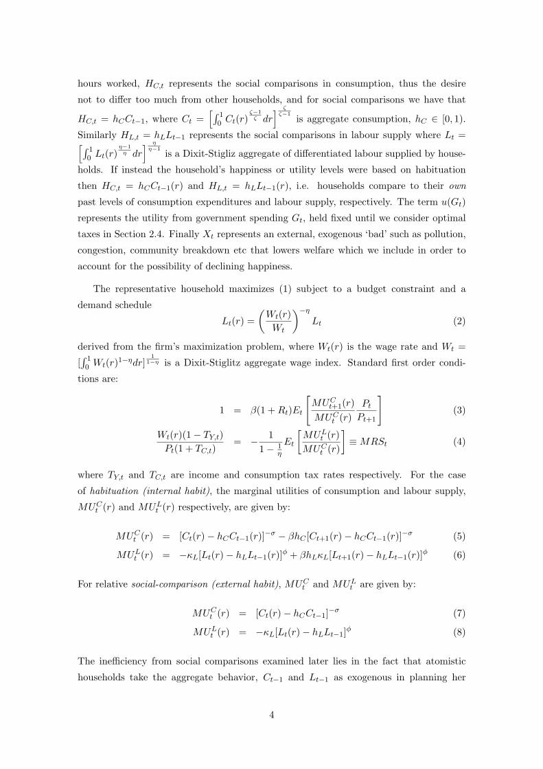
hours worked, HC,t represents the social comparisons in consumption, thus the desire

not to differ too much from other households, and for social comparisons we have that

HC,t = hCCt−1, where Ct =[∫ 1

0 Ct(r)ζ−1ζ dr

] ζζ−1

is aggregate consumption, hC ∈ [0, 1).

Similarly HL,t = hLLt−1 represents the social comparisons in labour supply where Lt =[∫ 10 Lt(r)

η−1η dr

] ηη−1

is a Dixit-Stigliz aggregate of differentiated labour supplied by house-

holds. If instead the household’s happiness or utility levels were based on habituation

then HC,t = hCCt−1(r) and HL,t = hLLt−1(r), i.e. households compare to their own

past levels of consumption expenditures and labour supply, respectively. The term u(Gt)

represents the utility from government spending Gt, held fixed until we consider optimal

taxes in Section 2.4. Finally Xt represents an external, exogenous ‘bad’ such as pollution,

congestion, community breakdown etc that lowers welfare which we include in order to

account for the possibility of declining happiness.

The representative household maximizes (1) subject to a budget constraint and a

demand schedule

Lt(r) =(Wt(r)Wt

)−ηLt (2)

derived from the firm’s maximization problem, where Wt(r) is the wage rate and Wt =

[∫ 1

0 Wt(r)1−ηdr]1

1−η is a Dixit-Stiglitz aggregate wage index. Standard first order condi-

tions are:

1 = β(1 +Rt)Et

[MUCt+1(r)MUCt (r)

PtPt+1

](3)

Wt(r)(1− TY,t)Pt(1 + TC,t)

= − 11− 1

η

Et

[MULt (r)MUCt (r)

]≡MRSt (4)

where TY,t and TC,t are income and consumption tax rates respectively. For the case

of habituation (internal habit), the marginal utilities of consumption and labour supply,

MUCt (r) and MULt (r) respectively, are given by:

MUCt (r) = [Ct(r)− hCCt−1(r)]−σ − βhC [Ct+1(r)− hCCt−1(r)]−σ (5)

MULt (r) = −κL[Lt(r)− hLLt−1(r)]φ + βhLκL[Lt+1(r)− hLLt−1(r)]φ (6)

For relative social-comparison (external habit), MUCt and MULt are given by:

MUCt (r) = [Ct(r)− hCCt−1]−σ (7)

MULt (r) = −κL[Lt(r)− hLLt−1]φ (8)

The inefficiency from social comparisons examined later lies in the fact that atomistic

households take the aggregate behavior, Ct−1 and Lt−1 as exogenous in planning her

4

lifetime consumption and labour supply. In fact the internal habit case reduces to that

with external habit if household fail to perceive the effect.3

In (3), the Keynes-Ramsey condition, Rt is the nominal rate of interest. In (4) which

equates the marginal rate of substitution with the real disposable wage, TY,t is the income

tax rate and TC,t is the consumption tax rate. The mark-up 11− 1

η

reflects the market power

of the household in the labour market.

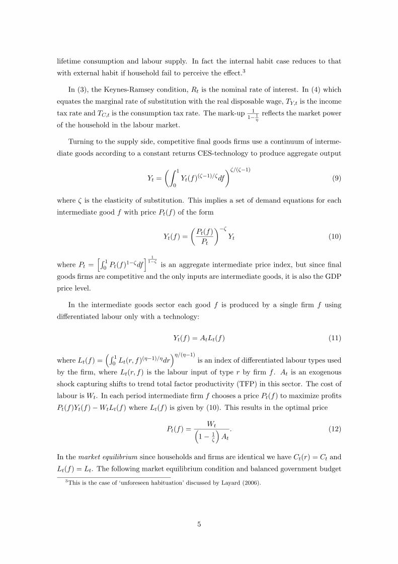
Turning to the supply side, competitive final goods firms use a continuum of interme-

diate goods according to a constant returns CES-technology to produce aggregate output

Yt =(∫ 1

0Yt(f)(ζ−1)/ζdf

)ζ/(ζ−1)

(9)

where ζ is the elasticity of substitution. This implies a set of demand equations for each

intermediate good f with price Pt(f) of the form

Yt(f) =(Pt(f)Pt

)−ζYt (10)

where Pt =[∫ 1

0 Pt(f)1−ζdf] 1

1−ζ is an aggregate intermediate price index, but since final

goods firms are competitive and the only inputs are intermediate goods, it is also the GDP

price level.

In the intermediate goods sector each good f is produced by a single firm f using

differentiated labour only with a technology:

Yt(f) = AtLt(f) (11)

where Lt(f) =(∫ 1

0 Lt(r, f)(η−1)/ηdr)η/(η−1)

is an index of differentiated labour types used

by the firm, where Lt(r, f) is the labour input of type r by firm f . At is an exogenous

shock capturing shifts to trend total factor productivity (TFP) in this sector. The cost of

labour is Wt. In each period intermediate firm f chooses a price Pt(f) to maximize profits

Pt(f)Yt(f)−WtLt(f) where Lt(f) is given by (10). This results in the optimal price

Pt(f) =Wt(

1− 1ζ

)At. (12)

In the market equilibrium since households and firms are identical we have Ct(r) = Ct and

Lt(f) = Lt. The following market equilibrium condition and balanced government budget3This is the case of ‘unforeseen habituation’ discussed by Layard (2006).

5

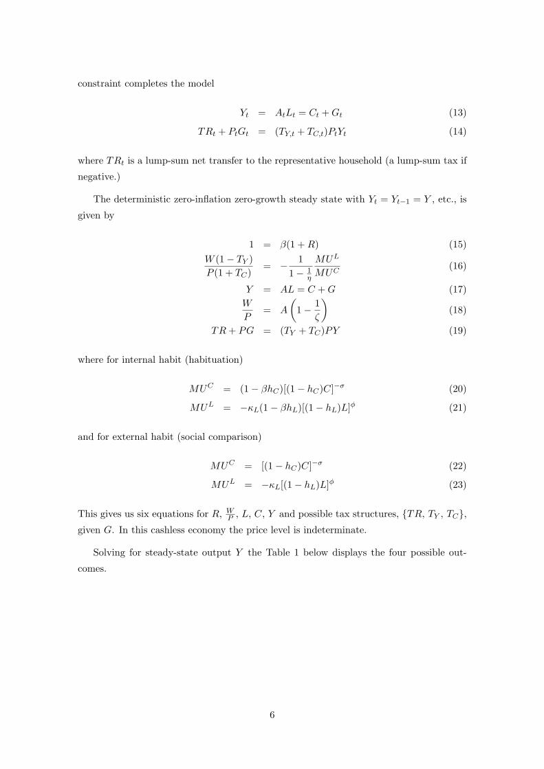
constraint completes the model

Yt = AtLt = Ct +Gt (13)

TRt + PtGt = (TY,t + TC,t)PtYt (14)

where TRt is a lump-sum net transfer to the representative household (a lump-sum tax if

negative.)

The deterministic zero-inflation zero-growth steady state with Yt = Yt−1 = Y , etc., is

given by

1 = β(1 +R) (15)W (1− TY )P (1 + TC)

= − 11− 1

η

MUL

MUC(16)

Y = AL = C +G (17)W

P= A

(1− 1

ζ

)(18)

TR+ PG = (TY + TC)PY (19)

where for internal habit (habituation)

MUC = (1− βhC)[(1− hC)C]−σ (20)

MUL = −κL(1− βhL)[(1− hL)L]φ (21)

and for external habit (social comparison)

MUC = [(1− hC)C]−σ (22)

MUL = −κL[(1− hL)L]φ (23)

This gives us six equations for R, WP , L, C, Y and possible tax structures, TR, TY , TC,given G. In this cashless economy the price level is indeterminate.

Solving for steady-state output Y the Table 1 below displays the four possible out-

comes.

6

Table 1: Equilibrium conditions in the Simple Model

Labour supply

Internal habit/Habituation

External habit/Social comparison

Consumption

Internal habit/Habituation Γ = Υ1−βhC

1−βhL Γ = Υ(1− βhC)

External habit/Social comparison

Γ = Υ 11−βhL Γ = Υ

where

Γ ≡(

1− G

Y

)σY φ+σ

Υ ≡(1− TY )

(1− 1

η

)(1− 1

ζ

)A1+φ

κL(1 + TC)(1− hL)φ(1− hC)σ

The market equilibrium in the steady state, given G, is then characterized by Y,C, Lgiven by (17), and the respective conditions in Table 1 with possible tax structures

TR, TY , TC satisfying the government budget constraint (19).4

2.2 Inefficiency and the Social Optimum

To examine the inefficiency of this deterministic steady state we consider the social plan-

ner’s problem obtained by maximizing

W0 =∞∑t=0

βt

[(Ct − hCCt−1)1−σ

1− σ− κL

(Lt − hLLt−1)1+φ

1 + φ− κX

X1+ϕt

1 + ϕ+ u(Gt)

](24)

with respect to Ct, Lt and Gt subject to the resource constraint:

Yt = AtLt = Ct +Gt

By analogy with private consumption we specialize the function u(Gt) by assuming

u(Gt) = κG(Gt − hGGt−1)1−σ

1− σ(25)

4The ‘tax wedge’ is 1+TY1−TC

− 1 ' TY + TC for small tax rates.

7

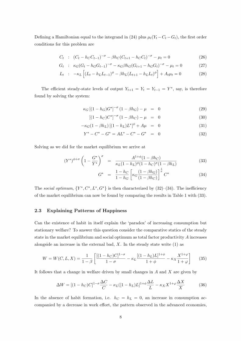
Defining a Hamiltonian equal to the integrand in (24) plus µt(Yt−Ct−Gt), the first order

conditions for this problem are

Ct : (Ct − hCCt−1)−σ − βhC(Ct+1 − hCCt)−σ − µt = 0 (26)

Gt : κG(Gt − hGGt−1)−σ − κGβhG(Gt+1 − hGGt)−σ − µt = 0 (27)

Lt : −κL[(Lt − hLLt−1)φ − βhL(Lt+1 − hLLt)φ

]+Atµt = 0 (28)

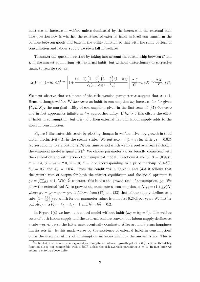
The efficient steady-state levels of output Yt+1 = Yt = Yt−1 = Y ∗, say, is therefore

found by solving the system:

κG [(1− hG)G∗]−σ (1− βhG)− µ = 0 (29)

[(1− hC)C∗]−σ (1− βhC)− µ = 0 (30)

−κG(1− βhL) [(1− hL)L∗]φ +Aµ = 0 (31)

Y ∗ − C∗ −G∗ = AL∗ − C∗ −G∗ = 0 (32)

Solving as we did for the market equilibrium we arrive at

(Y ∗)φ+σ

(1− G∗

Y ∗

)σ=

A1+φ(1− βhC)κL(1− hL)φ(1− hC)σ(1− βhL)

(33)

G∗ =1− hC1− hG

[κG

(1− βhG)(1− βhC)

] 1σ

C∗ (34)

The social optimum, Y ∗, C∗, L∗, G∗ is then characterized by (32)–(34). The inefficiency

of the market equilibrium can now be found by comparing the results in Table 1 with (33).

2.3 Explaining Patterns of Happiness

Can the existence of habit in itself explain the ‘paradox’ of increasing consumption but

stationary welfare? To answer this question consider the comparative statics of the steady

state in the market equilibrium and social optimum as total factor productivity A increases

alongside an increase in the external bad, X. In the steady state write (1) as

W = W (C,L,X) =1

1− β

[[(1− hC)C]1−σ

1− σ− κL

[(1− hL)L]1+φ

1 + φ− κX

X1+ϕ

1 + ϕ

](35)

It follows that a change in welfare driven by small changes in A and X are given by

∆W = [(1− hC)C]1−σ∆CC− κL([1− hL)L]1+φ∆L

L− κXX1+ϕ∆X

X(36)

In the absence of habit formation, i.e. hC = hL = 0, an increase in consumption ac-

companied by a decrease in work effort, the pattern observed in the advanced economies,

8

must see an increase in welfare unless dominated by the increase in the external bad.

The question now is whether the existence of external habit in itself can transform the

balance between goods and bads in the utility function so that with the same pattern of

consumption and labour supply we see a fall in welfare?

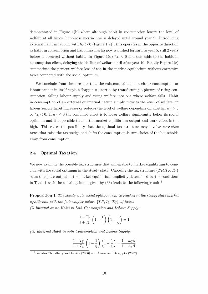
To answer this question we start by taking into account the relationship between C and

L in the market equilibrium with external habit, but without distortionary or corrective

taxes, to rewrite (36) as

∆W = [(1−hC)C]1−σ

1 +(σ − 1)

(1− 1

ζ

)(1− 1

η

)(1− hL)

cy(1 + φ)(1− hC)

∆CC−κXX1+ϕ∆X

X. (37)

We next observe that estimates of the risk aversion parameter σ suggest that σ > 1.

Hence although welfare W decreases as habit in consumption hC increases for for given

C,L,X, the marginal utility of consumption, given in the first term of (37) increases

and in fact approaches infinity as hC approaches unity. If hL > 0 this offsets the effect

of habit in consumption, but if hL < 0 then external habit in labour supply adds to the

effect in consumption.

Figure 1 illustrates this result by plotting changes in welfare driven by growth in total

factor productivity At in the steady state. We put at+1 = (1 + gA)at with gA = 0.025

(corresponding to a growth of 2.5% per time period which we interpret as a year (although

the empirical model is quarterly).5 We choose parameter values broadly consistent with

the calibration and estimation of our empirical model in sections 4 and 5: β = (0.99)4,

σ = 1.4, φ = ϕ = 2.0, η = 3, ζ = 7.65 (corresponding to a price mark-up of 15%),

hC = 0.7 and hL = ±0.5. From the conditions in Table 1 and (33) it follows that

the growth rate of output for both the market equilibrium and the social optimum is

gY = 1+φφ+σgA < 1. With G

Y constant, this is also the growth rate of consumption, gC . We

allow the external bad Xt to grow at the same rate as consumption so Xt+1 = (1 + gX)Xt

where gX = gC = gY = gG. It follows from (17) and (33) that labour supply declines at a

rate(

1− 1+φφ+σ

)gA which for our parameter values is a modest 0.29% per year. We further

put A(0) = X(0) = kL = kG = 1 and GY = G∗

Y ∗ = 0.2.

In Figure 1(a) we have a standard model without habit (hC = hL = 0). The welfare

costs of both labour supply and the external bad are convex, but labour supply declines at

a rate −gL gX so the latter must eventually dominate. After around 3 years happiness

inertia sets in. Is this made worse by the existence of external habit in consumption?

Since the marginal utility of consumption increases with hC the answer is no. This is5Note that this cannot be interpreted as a long-term balanced growth path (BGP) because the utility

function (1) is not compatible with a BGP unless the risk aversion parameter σ = 1. In fact later weestimate σ to be above unity.

9

demonstrated in Figure 1(b) where although habit in consumption lowers the level of

welfare at all times, happiness inertia now is delayed until around year 9. Introducing

external habit in labour, with hL > 0 (Figure 1(c)), this operates in the opposite direction

as habit in consumption and happiness inertia now is pushed forward to year 5, still 2 years

before it occurred without habit. In Figure 1(d) hL < 0 and this adds to the habit in

consumption effect, delaying the decline of welfare until after year 10. Finally Figure 1(e)

summarizes the percent welfare loss of the in the market equilibrium without corrective

taxes compared with the social optimum.

We conclude from these results that the existence of habit in either consumption or

labour cannot in itself explain ‘happiness-inertia’ by transforming a picture of rising con-

sumption, falling labour supply and rising welfare into one where welfare falls. Habit

in consumption of an external or internal nature simply reduces the level of welfare; in

labour supply habit increases or reduces the level of welfare depending on whether hL > 0

or hL < 0. If hL ≤ 0 the combined effect is to lower welfare significantly below its social

optimum and it is possible that in the market equilibrium output and work effort is too

high. This raises the possibility that the optimal tax structure may involve corrective

taxes that raise the tax wedge and shifts the consumption-leisure choice of the households

away from consumption.

2.4 Optimal Taxation

We now examine the possible tax structures that will enable to market equilibrium to coin-

cide with the social optimum in the steady state. Choosing the tax structure TR, TY , TCso as to equate output in the market equilibrium implicitly determined by the conditions

in Table 1 with the social optimum given by (33) leads to the following result:6

Proposition 1 The steady state social optimum can be reached in the steady state market

equilibrium with the following structure TR, TY , TC of taxes:

(i) Internal or no Habit in both Consumption and Labour Supply:

1− TY1 + TC

(1− 1

η

)(1− 1

ζ

)= 1

(ii) External Habit in both Consumption and Labour Supply:

1− TY1 + TC

(1− 1

η

)(1− 1

ζ

)=

1− hCβ1− hLβ

6See also Choudhary and Levine (2006) and Arrow and Dasgupta (2007).

10

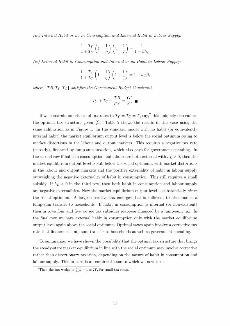
(iii) Internal Habit or no in Consumption and External Habit in Labour Supply:

1− TY1 + TC

(1− 1

η

)(1− 1

ζ

)=

11− βhL

(iv) External Habit in Consumption and Internal or no Habit in Labour Supply:

1− TY1 + TC

(1− 1

η

)(1− 1

ζ

)= 1− hCβ,

where TR, TY , TC satisfies the Government Budget Constraint

TY + TC −TR

PY=G∗

Y ∗

If we constrain our choice of tax rates to TY = TC = T , say,7 this uniquely determines

the optimal tax structure given G∗

Y ∗ . Table 2 shows the results in this case using the

same calibration as in Figure 1. In the standard model with no habit (or equivalently

internal habit) the market equilibrium output level is below the social optimum owing to

market distortions in the labour and output markets. This requires a negative tax rate

(subsidy), financed by lump-sum taxation, which also pays for government spending. In

the second row if habit in consumption and labour are both external with hL > 0, then the

market equilibrium output level is still below the social optimum, with market distortions

in the labour and output markets and the positive externality of habit in labour supply

outweighing the negative externality of habit in consumption. This still requires a small

subsidy. If hL < 0 in the third row, then both habit in consumption and labour supply

are negative externalities. Now the market equilibrium output level is substantially above

the social optimum. A large corrective tax emerges that is sufficient to also finance a

lump-sum transfer to households. If habit in consumption is internal (or non-existent)

then in rows four and five we see tax subsidies reappear financed by a lump-sum tax. In

the final row we have external habit in consumption only with the market equilibrium

output level again above the social optimum. Optimal taxes again involve a corrective tax

rate that finances a lump-sum transfer to households as well as government spending.

To summarize: we have shown the possibility that the optimal tax structure that brings

the steady-state market equilibrium in line with the social optimum may involve corrective

rather than distortionary taxation, depending on the nature of habit in consumption and

labour supply. This in turn is an empirical issue to which we now turn.7Then the tax wedge is 1+T

1−T − 1 ' 2T , for small tax rates.

11

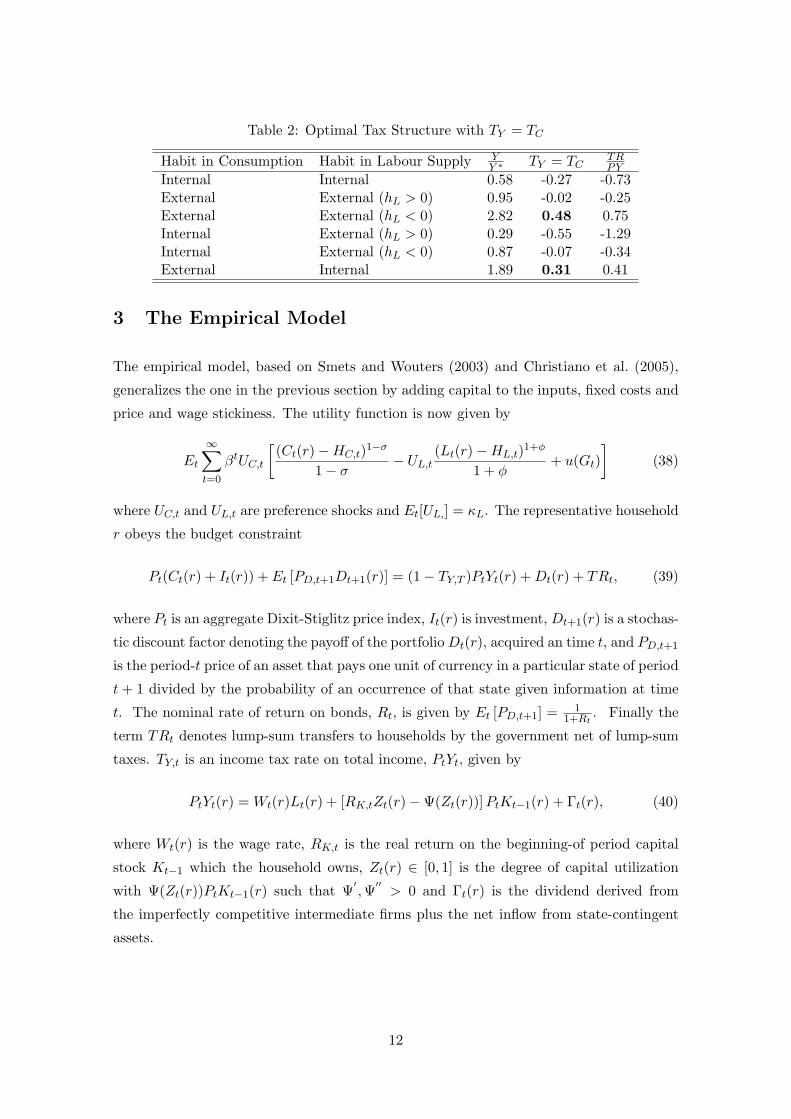
Table 2: Optimal Tax Structure with TY = TC

Habit in Consumption Habit in Labour Supply YY ∗ TY = TC

TRPY

Internal Internal 0.58 -0.27 -0.73External External (hL > 0) 0.95 -0.02 -0.25External External (hL < 0) 2.82 0.48 0.75Internal External (hL > 0) 0.29 -0.55 -1.29Internal External (hL < 0) 0.87 -0.07 -0.34External Internal 1.89 0.31 0.41

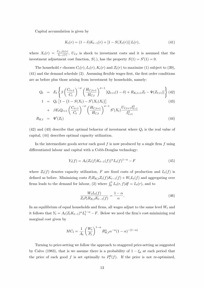
3 The Empirical Model

The empirical model, based on Smets and Wouters (2003) and Christiano et al. (2005),

generalizes the one in the previous section by adding capital to the inputs, fixed costs and

price and wage stickiness. The utility function is now given by

Et

∞∑t=0

βtUC,t

[(Ct(r)−HC,t)1−σ

1− σ− UL,t

(Lt(r)−HL,t)1+φ

1 + φ+ u(Gt)

](38)

where UC,t and UL,t are preference shocks and Et[UL,] = κL. The representative household

r obeys the budget constraint

Pt(Ct(r) + It(r)) + Et [PD,t+1Dt+1(r)] = (1− TY,T )PtYt(r) +Dt(r) + TRt, (39)

where Pt is an aggregate Dixit-Stiglitz price index, It(r) is investment, Dt+1(r) is a stochas-

tic discount factor denoting the payoff of the portfolioDt(r), acquired an time t, and PD,t+1

is the period-t price of an asset that pays one unit of currency in a particular state of period

t + 1 divided by the probability of an occurrence of that state given information at time

t. The nominal rate of return on bonds, Rt, is given by Et [PD,t+1] = 11+Rt

. Finally the

term TRt denotes lump-sum transfers to households by the government net of lump-sum

taxes. TY,t is an income tax rate on total income, PtYt, given by

PtYt(r) = Wt(r)Lt(r) + [RK,tZt(r)−Ψ(Zt(r))]PtKt−1(r) + Γt(r), (40)

where Wt(r) is the wage rate, RK,t is the real return on the beginning-of period capital

stock Kt−1 which the household owns, Zt(r) ∈ [0, 1] is the degree of capital utilization

with Ψ(Zt(r))PtKt−1(r) such that Ψ′,Ψ′′> 0 and Γt(r) is the dividend derived from

the imperfectly competitive intermediate firms plus the net inflow from state-contingent

assets.

12

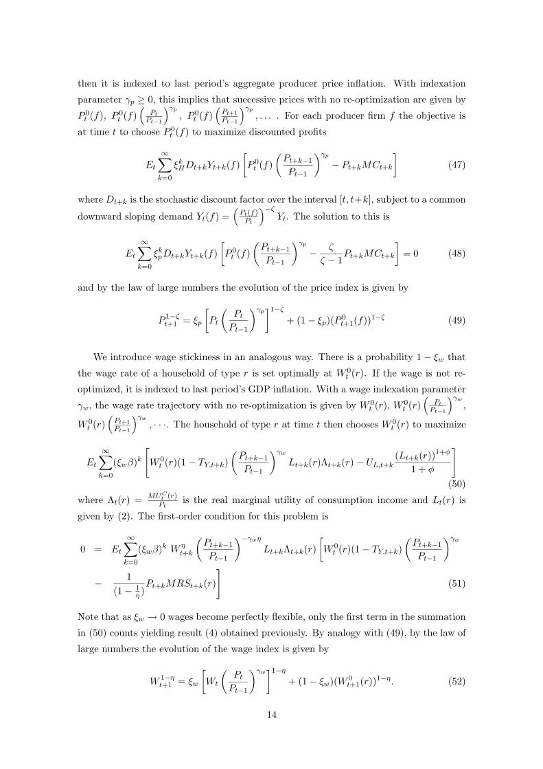
Capital accumulation is given by

Kt(r) = (1− δ)Kt−1(r) + [1− S(Xt(r))] It(r), (41)

where Xt(r) = UI,tIt(r)It−1(r) , UI,t is shock to investment costs and it is assumed that the

investment adjustment cost function, S(.), has the property S(1) = S′(1) = 0.

The household r chooses Ct(r), Lt(r),Kt(r) and Zt(r) to maximize (1) subject to (39),

(41) and the demand schedule (2). Assuming flexible wages first, the first order conditions

are as before plus those arising from investment by households, namely:

Qt = Et

β

(Ct+1

Ct

)−σ (HC,t+1

HC,t

)σ−1

[Qt+1(1− δ) +RK,t+1Zt −Ψ(Zt+1)]

(42)

1 = Qt[1−

(1− S(Xt)− S′(Xt)Xt

)](43)

+ βEtQt+1

(Ct+1

Ct

)−σ (HC,t+1

HC,t

)σ−1

S′(Xt)UI,t+1I

2t+1

I2t+1

RK,t = Ψ′(Zt) (44)

(42) and (43) describe that optimal behavior of investment where Qt is the real value of

capital, (44) describes optimal capacity utilization.

In the intermediate goods sector each good f is now produced by a single firm f using

differentiated labour and capital with a Cobb-Douglas technology:

Yt(f) = At(Zt(f)Kt−1(f))αLt(f)1−α − F (45)

where Zt(f) denotes capacity utilization, F are fixed costs of production and Lt(f) is

defined as before. Minimizing costs PtRK,tZt(f)Kt−1(f) +WtLt(f) and aggregating over

firms leads to the demand for labour, (2) where∫ 1

0 Lt(r, f)df = Lt(r), and to

WtLt(f)ZtPtRK,tKt−1(f)

=1− αα

. (46)

In an equilibrium of equal households and firms, all wages adjust to the same level Wt and

it follows that Yt = At(ZtKt−1)αL1−αt −F . Below we need the firm’s cost-minimizing real

marginal cost given by

MCt =1At

(Wt

Pt

)1−αRαK,tα

−α(1− α)−(1−α)

Turning to price-setting we follow the approach to staggered price-setting as suggested

by Calvo (1983), that is we assume there is a probability of 1 − ξp at each period that

the price of each good f is set optimally to P 0t (f). If the price is not re-optimized,

13

then it is indexed to last period’s aggregate producer price inflation. With indexation

parameter γp ≥ 0, this implies that successive prices with no re-optimization are given by

P 0t (f), P 0

t (f)(

PtPt−1

)γp, P 0

t (f)(Pt+1

Pt−1

)γp, . . . . For each producer firm f the objective is

at time t to choose P 0t (f) to maximize discounted profits

Et

∞∑k=0

ξkHDt+kYt+k(f)[P 0t (f)

(Pt+k−1

Pt−1

)γp− Pt+kMCt+k

](47)

where Dt+k is the stochastic discount factor over the interval [t, t+k], subject to a common

downward sloping demand Yt(f) =(Pt(f)Pt

)−ζYt. The solution to this is

Et

∞∑k=0

ξkpDt+kYt+k(f)[P 0t (f)

(Pt+k−1

Pt−1

)γp− ζ

ζ − 1Pt+kMCt+k

]= 0 (48)

and by the law of large numbers the evolution of the price index is given by

P 1−ζt+1 = ξp

[Pt

(PtPt−1

)γp]1−ζ+ (1− ξp)(P 0

t+1(f))1−ζ (49)

We introduce wage stickiness in an analogous way. There is a probability 1− ξw that

the wage rate of a household of type r is set optimally at W 0t (r). If the wage is not re-

optimized, it is indexed to last period’s GDP inflation. With a wage indexation parameter

γw, the wage rate trajectory with no re-optimization is given by W 0t (r), W 0

t (r)(

PtPt−1

)γw,

W 0t (r)

(Pt+1

Pt−1

)γw, · · ·. The household of type r at time t then chooses W 0

t (r) to maximize

Et

∞∑k=0

(ξwβ)k[W 0t (r)(1− TY,t+k)

(Pt+k−1

Pt−1

)γwLt+k(r)Λt+k(r)− UL,t+k

(Lt+k(r))1+φ

1 + φ

](50)

where Λt(r) = MUCt (r)Pt

is the real marginal utility of consumption income and Lt(r) is

given by (2). The first-order condition for this problem is

0 = Et

∞∑k=0

(ξwβ)k W ηt+k

(Pt+k−1

Pt−1

)−γwηLt+kΛt+k(r)

[W 0t (r)(1− TY,t+k)

(Pt+k−1

Pt−1

)γw− 1

(1− 1η )Pt+kMRSt+k(r)

](51)

Note that as ξw → 0 wages become perfectly flexible, only the first term in the summation

in (50) counts yielding result (4) obtained previously. By analogy with (49), by the law of

large numbers the evolution of the wage index is given by

W 1−ηt+1 = ξw

[Wt

(PtPt−1

)γw]1−η+ (1− ξw)(W 0

t+1(r))1−η. (52)

14

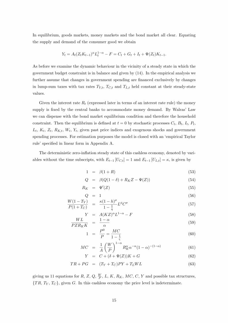
In equilibrium, goods markets, money markets and the bond market all clear. Equating

the supply and demand of the consumer good we obtain

Yt = At(ZtKt−1)αL1−αt − F = Ct +Gt + It + Ψ(Zt)Kt−1.

As before we examine the dynamic behaviour in the vicinity of a steady state in which the

government budget constraint is in balance and given by (14). In the empirical analysis we

further assume that changes in government spending are financed exclusively by changes

in lump-sum taxes with tax rates TY,t, TC,t and TL,t held constant at their steady-state

values.

Given the interest rate Rt (expressed later in terms of an interest rate rule) the money

supply is fixed by the central banks to accommodate money demand. By Walras’ Law

we can dispense with the bond market equilibrium condition and therefore the household

constraint. Then the equilibrium is defined at t = 0 by stochastic processes Ct, Bt, It, Pt,

Lt, Kt, Zt, RK,t, Wt, Yt, given past price indices and exogenous shocks and government

spending processes. For estimation purposes the model is closed with an ‘empirical Taylor

rule’ specified in linear form in Appendix A.

The deterministic zero-inflation steady state of this cashless economy, denoted by vari-

ables without the time subscripts, with Et−1 [UC,t] = 1 and Et−1 [UL,t] = κ, is given by

1 = β(1 +R) (53)

Q = β(Q(1− δ) +RKZ −Ψ(Z)) (54)

RK = Ψ′(Z) (55)

Q = 1 (56)W (1− TY )P (1 + TC)

=κ(1− h)σ

1− 1η

LφCσ (57)

Y = A(KZ)αL1−α − F (58)WL

PZRKK=

1− αα

(59)

1 =P 0

P=

MC

1− 1ζ

(60)

MC =1A

(W

P

)1−αRαKα

−α(1− α)−(1−α) (61)

Y = C + (δ + Ψ(Z))K +G (62)

TR+ PG = (TY + TC)PY + TLWL (63)

giving us 11 equations for R, Z, Q, WP , L, K, RK , MC, C, Y and possible tax structures,

TR, TY , TC, given G. In this cashless economy the price level is indeterminate.

15

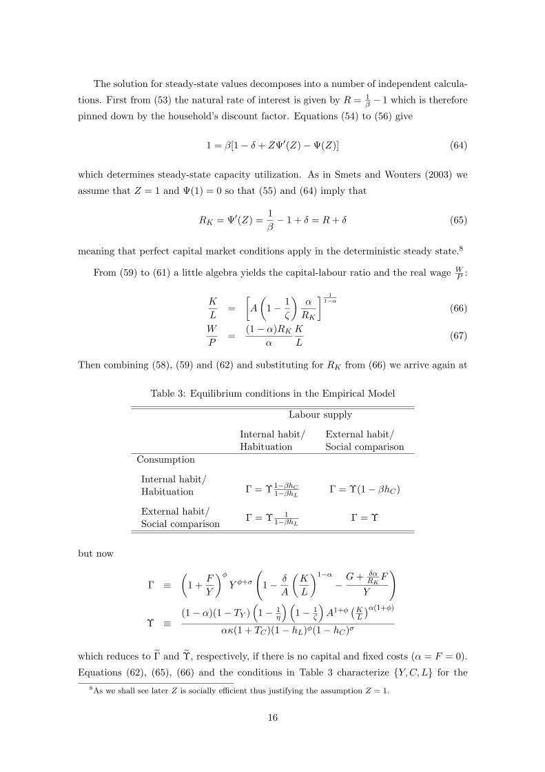
The solution for steady-state values decomposes into a number of independent calcula-

tions. First from (53) the natural rate of interest is given by R = 1β − 1 which is therefore

pinned down by the household’s discount factor. Equations (54) to (56) give

1 = β[1− δ + ZΨ′(Z)−Ψ(Z)] (64)

which determines steady-state capacity utilization. As in Smets and Wouters (2003) we

assume that Z = 1 and Ψ(1) = 0 so that (55) and (64) imply that

RK = Ψ′(Z) =1β− 1 + δ = R+ δ (65)

meaning that perfect capital market conditions apply in the deterministic steady state.8

From (59) to (61) a little algebra yields the capital-labour ratio and the real wage WP :

K

L=

[A

(1− 1

ζ

)α

RK

] 11−α

(66)

W

P=

(1− α)RKα

K

L(67)

Then combining (58), (59) and (62) and substituting for RK from (66) we arrive again at

Table 3: Equilibrium conditions in the Empirical Model

Labour supply

Internal habit/Habituation

External habit/Social comparison

Consumption

Internal habit/Habituation Γ = Υ1−βhC

1−βhL Γ = Υ(1− βhC)

External habit/Social comparison

Γ = Υ 11−βhL Γ = Υ

but now

Γ ≡(

1 +F

Y

)φY φ+σ

(1− δ

A

(K

L

)1−α−G+ δα

RKF

Y

)

Υ ≡(1− α)(1− TY )

(1− 1

η

)(1− 1

ζ

)A1+φ

(KL

)α(1+φ)

ακ(1 + TC)(1− hL)φ(1− hC)σ

which reduces to Γ and Υ, respectively, if there is no capital and fixed costs (α = F = 0).

Equations (62), (65), (66) and the conditions in Table 3 characterize Y,C, L for the8As we shall see later Z is socially efficient thus justifying the assumption Z = 1.

16

steady state of the market equilibrium of the empirical model.

3.1 Inefficiency in the Empirical Model

The social planner’s problem for the deterministic case is now obtained by maximizing

Ω0 =∞∑t=0

βt[

(Ct − hCCt−1)1−σ

1− σ− κG

(Lt − hLLt−1)1+φ

1 + φ+ u(Gt)

]

with respect to Ct, Kt, Lt and Zt subject to the resource constraint:

Yt = At(ZtKt−1)αL1−αt = Ct +Gt +Kt − (1− δ)Kt−1 + Ψ(Zt)Kt−1

Solving this problem as for the model with no capital we arrive at

1 = β[1− δ + Z∗Ψ′(Z∗)−Ψ(Z∗)] (68)

Hence Z∗ = Z = 1 and R∗K = RK = R+ δ = 1β − 1 + δ. Thus the market rate of capacity

utilization is efficient. However,

K∗

L∗=[Aα

RK

] 11−α

>K

L=[(

1− 1ζ

)Aα

RK

] 11−α

(69)

and the market capital-labour ratio is below the social optimum. The socially optimal level

of output is now found from

(1 +

F ∗

Y ∗

)φ(Y ∗)φ+σ

[1− δ

A

(K∗

L∗

)1−α−G∗ + δα

RKF ∗

Y ∗

]σ

=(1− α)A1+φ

(K∗

L∗

)α(1+φ)(1− βhC)

ακ(1− hL)φ(1− hC)σ(1− βhL)(70)

The inefficiency of the natural rate of output can now be found by comparing the

results in Table 3 with (70). Since Y φ+δ is an increasing function of Y , we arrive at9

9This generalizes the result in Choudhary and Levine (2006) which considered the same model, butwithout capital as in Section 2.

17

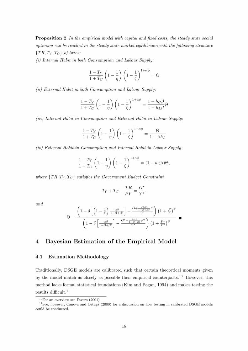
Proposition 2 In the empirical model with capital and fixed costs, the steady state social

optimum can be reached in the steady state market equilibrium with the following structure

TR, TY , TC of taxes:

(i) Internal Habit in both Consumption and Labour Supply:

1− TY1 + TC

(1− 1

η

)(1− 1

ζ

)1+αφ

= Θ

(ii) External Habit in both Consumption and Labour Supply:

1− TY1 + TC

(1− 1

η

)(1− 1

ζ

)1+αφ

=1− hCβ1− hLβ

Θ

(iii) Internal Habit in Consumption and External Habit in Labour Supply:

1− TY1 + TC

(1− 1

η

)(1− 1

ζ

)1+αφ

=Θ

1− βhL

(iv) External Habit in Consumption and Internal Habit in Labour Supply:

1− TY1 + TC

(1− 1

η

)(1− 1

ζ

)1+αφ

= (1− hCβ)Θ,

where TR, TY , TC satisfies the Government Budget Constraint

TY + TC −TR

PY=G∗

Y ∗.

and

Θ =

(1− δ

[(1− 1

ζ

)αβ

1−β+βδ

]−

G+ δαβ1−β+βδ

F

Y

)(1 + F

Y

)φ(

1− δ[

αβ1−β+βδ

]−

G∗+ δαβ1−β+βδ

F ∗

Y ∗

)(1 + F ∗

Y ∗

)φ

4 Bayesian Estimation of the Empirical Model

4.1 Estimation Methodology

Traditionally, DSGE models are calibrated such that certain theoretical moments given

by the model match as closely as possible their empirical counterparts.10 However, this

method lacks formal statistical foundations (Kim and Pagan, 1994) and makes testing the

results difficult.11

10For an overview see Favero (2001).11See, however, Canova and Ortega (2000) for a discussion on how testing in calibrated DSGE models

could be conducted.

18

Following Sargent (1989), and preceding the Bayesian literature, the common praxis

was to estimate DSGE models with maximum likelihood (ML). For instance McGrattan

(1994) analyzes the effects of taxation in an estimated business cycle model and Leeper and

Sims (1994) and Kim (2000) estimated DSGE models for the analysis of monetary policy.

Well known problems arising with this method are that parameters take on corner solutions

or implausible values, and that the likelihood function may be flat in some dimensions.

GMM estimation is a popular alternative for estimating intertemporal models (Galı and

Gertler, 1999). However, Christiano and Haan (1996) show by estimating a business cycle

model on U.S. data that GMM estimators often do not have the distributions implied

by asymptotic theory. In addition, Linde (2005) finds that parameters in a simple New

Keynesian model are likely to be estimated imprecisely and with bias.

The Bayesian approach taken in this paper follows work by DeJong et al. (2000a,b),

Otrok (2001), Smets and Wouters (2003) 12 and can be seen as a combination of likelihood

methods and the calibration methodology. Bayesian analysis allows formally incorporating

uncertainty and prior information regarding the parametrisation of the model by combin-

ing the likelihood with a prior density for the parameters of interest. The moments of the

prior density can be based on results from earlier microeconometric or macroeconometric

studies, that is appropriate values could be employed as the means or modes of the prior

density, while a priori uncertainty can be expressed by choosing the appropriate prior

variance. For example, the restriction that AR(1)-coefficients lie within the unit interval

can be implemented by choosing a prior density that covers only that interval, such as a

truncated normal or a beta density. This strategy may help to mitigate numerical prob-

lems stemming e.g. from a flat likelihood function as estimates of the maximum likelihood

are pulled towards values that the researcher would consider sensible a priori. This effect

will be stronger when the data carry little information about a certain parameter, that is

the likelihood is relatively flat whereas the effect will only be moderate when the likelihood

is very peaked.

By Bayes’ theorem, the posterior density ϕ(ξ | Y ) is related to prior and likelihood as

follows

ϕ(ξ | Y ) =f(Y | ξ)π(ξ)

f(Y )∝ f(Y | ξ)π(ξ) = L(ξ | Y )π(ξ),

where π(ξ) denotes the prior density of the parameter vector ξ, L(ξ | Y ) ≡ f(Y | ξ) is

the likelihood of the sample Y and f(Y ) =∫f(Y | ξ)π(ξ)dξ is the unconditional sample

density. The unconditional sample density does not depend on the unknown parameters

and consequently serves only as a proportionality factor that can be neglected for estima-

tion purposes. In this context it becomes clear that the main difference between ‘classical’12There are by now numerous applications of the approach, for example Adolfson et al. (2005, 2007),

Justiniano and Preston (2004), Lubik and Schorfheide (2004) and Rabanal and Rubio-Ramırez (2005).

19

and Bayesian statistics is a matter of conditioning. Likelihood-based non-Bayesian meth-

ods condition on the unknown parameters ξ and compare f(Y | ξ) with the observed

data. Bayesian methods condition on the observed data and use the full distribution

f(ξ, Y ) = f(Y | ξ)π(ξ) and require specification of a prior density π(ξ).

Computation of the posterior distribution ϕ(ξ | Y ) requires calculating the likelihood

and then multiplying by the prior density. The likelihood function can be computed

with the Kalman filter using the state-space representation of the solution to the rational

expectations model. The method is explained in some detail in Appendix B.

4.2 Specification of Priors

In specifying the prior density for the parameter vector we assume that all parameters are

independently distributed of each other, i.e.

π(ξ) =n∏i=1

πi(ξi),

where ξi, i = 1, .., n denotes elements in ξ. 13

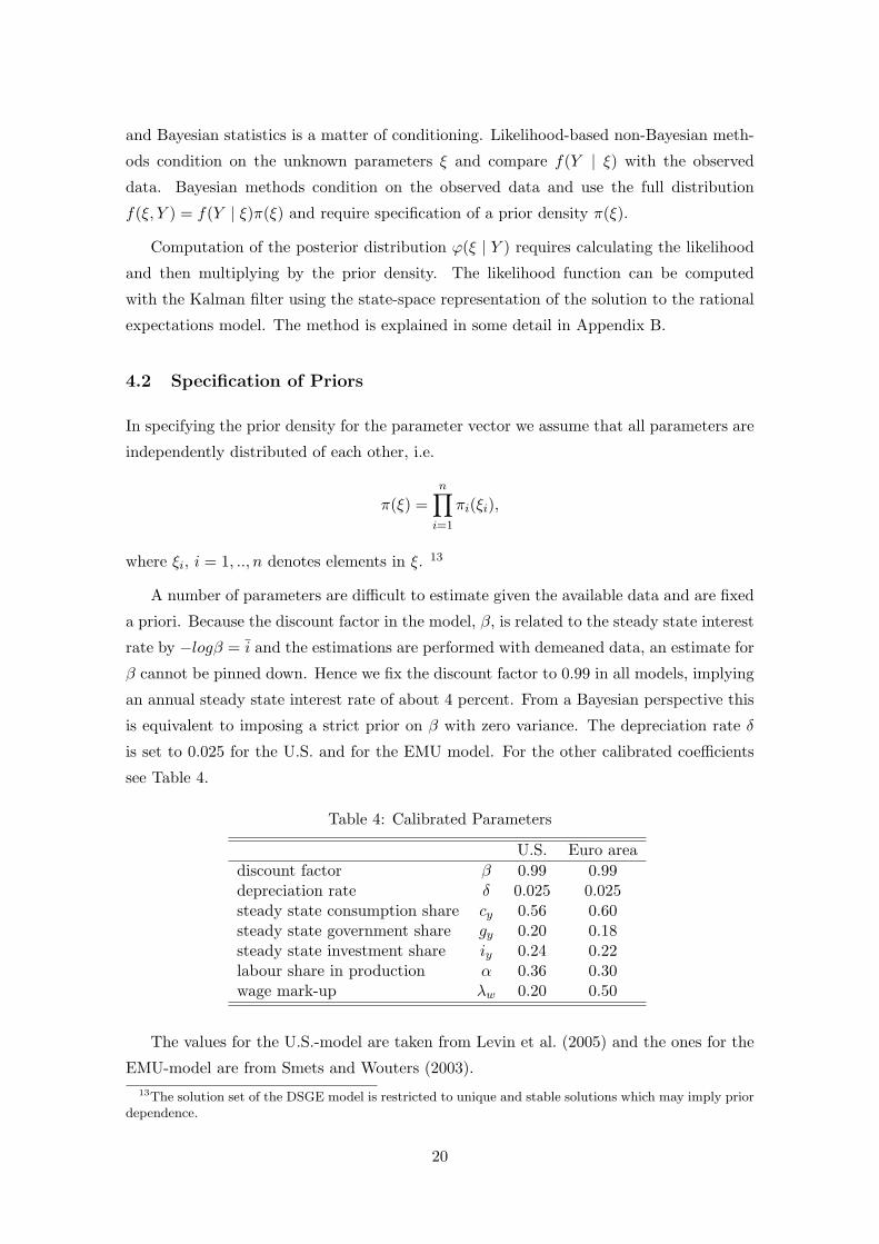
A number of parameters are difficult to estimate given the available data and are fixed

a priori. Because the discount factor in the model, β, is related to the steady state interest

rate by −logβ = i and the estimations are performed with demeaned data, an estimate for

β cannot be pinned down. Hence we fix the discount factor to 0.99 in all models, implying

an annual steady state interest rate of about 4 percent. From a Bayesian perspective this

is equivalent to imposing a strict prior on β with zero variance. The depreciation rate δ

is set to 0.025 for the U.S. and for the EMU model. For the other calibrated coefficients

see Table 4.

Table 4: Calibrated Parameters

U.S. Euro areadiscount factor β 0.99 0.99depreciation rate δ 0.025 0.025steady state consumption share cy 0.56 0.60steady state government share gy 0.20 0.18steady state investment share iy 0.24 0.22labour share in production α 0.36 0.30wage mark-up λw 0.20 0.50

The values for the U.S.-model are taken from Levin et al. (2005) and the ones for the

EMU-model are from Smets and Wouters (2003).13The solution set of the DSGE model is restricted to unique and stable solutions which may imply prior

dependence.

20

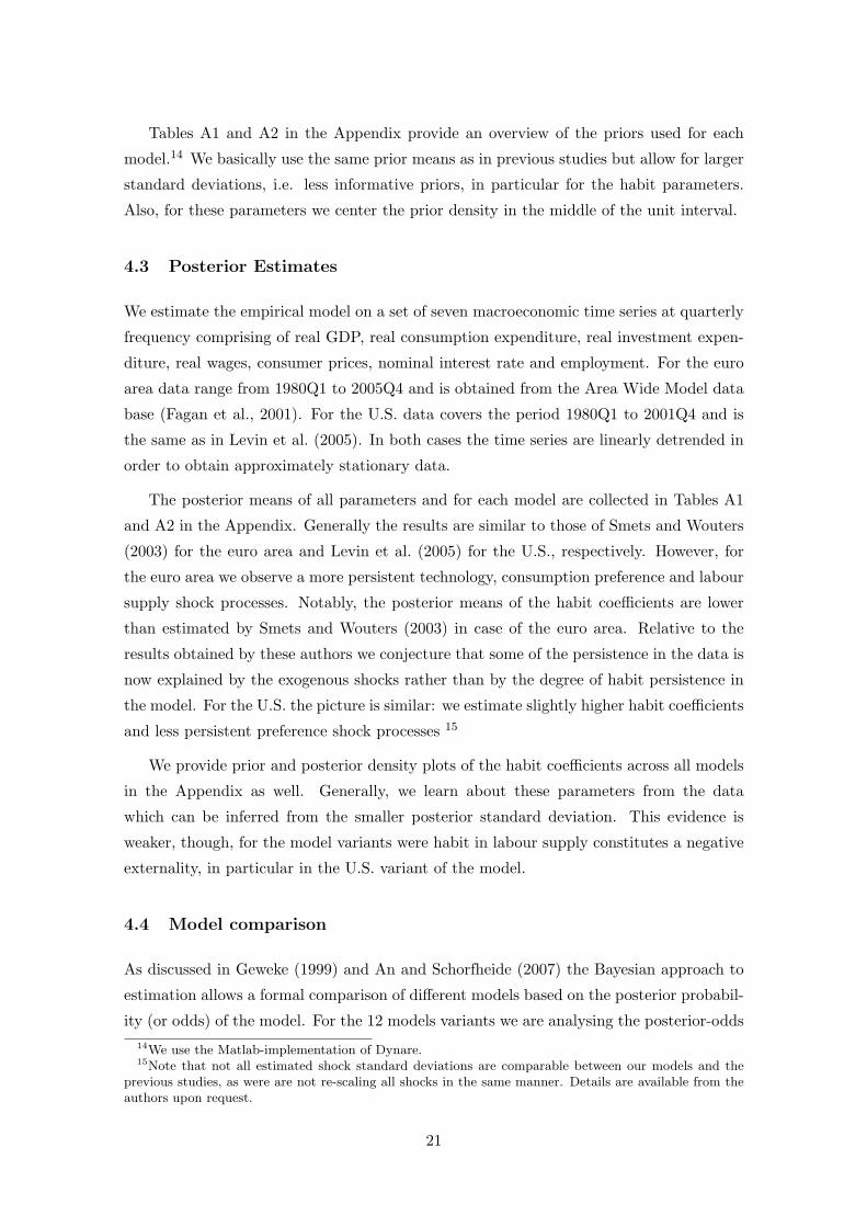
Tables A1 and A2 in the Appendix provide an overview of the priors used for each

model.14 We basically use the same prior means as in previous studies but allow for larger

standard deviations, i.e. less informative priors, in particular for the habit parameters.

Also, for these parameters we center the prior density in the middle of the unit interval.

4.3 Posterior Estimates

We estimate the empirical model on a set of seven macroeconomic time series at quarterly

frequency comprising of real GDP, real consumption expenditure, real investment expen-

diture, real wages, consumer prices, nominal interest rate and employment. For the euro

area data range from 1980Q1 to 2005Q4 and is obtained from the Area Wide Model data

base (Fagan et al., 2001). For the U.S. data covers the period 1980Q1 to 2001Q4 and is

the same as in Levin et al. (2005). In both cases the time series are linearly detrended in

order to obtain approximately stationary data.

The posterior means of all parameters and for each model are collected in Tables A1

and A2 in the Appendix. Generally the results are similar to those of Smets and Wouters

(2003) for the euro area and Levin et al. (2005) for the U.S., respectively. However, for

the euro area we observe a more persistent technology, consumption preference and labour

supply shock processes. Notably, the posterior means of the habit coefficients are lower

than estimated by Smets and Wouters (2003) in case of the euro area. Relative to the

results obtained by these authors we conjecture that some of the persistence in the data is

now explained by the exogenous shocks rather than by the degree of habit persistence in

the model. For the U.S. the picture is similar: we estimate slightly higher habit coefficients

and less persistent preference shock processes 15

We provide prior and posterior density plots of the habit coefficients across all models

in the Appendix as well. Generally, we learn about these parameters from the data

which can be inferred from the smaller posterior standard deviation. This evidence is

weaker, though, for the model variants were habit in labour supply constitutes a negative

externality, in particular in the U.S. variant of the model.

4.4 Model comparison

As discussed in Geweke (1999) and An and Schorfheide (2007) the Bayesian approach to

estimation allows a formal comparison of different models based on the posterior probabil-

ity (or odds) of the model. For the 12 models variants we are analysing the posterior-odds14We use the Matlab-implementation of Dynare.15Note that not all estimated shock standard deviations are comparable between our models and the

previous studies, as were are not re-scaling all shocks in the same manner. Details are available from theauthors upon request.

21

of model Mi is defined by

POi =pif(YT |Mi)∑

j=1,.....,12 pjf(YT |Mj), (71)

where pi and pj are the prior model probabilities assigned to be equal to 1/12 for each

model.

f(YT |Mi) denotes the marginal likelihood of a model i that is defined by

f(YT |Mi) =∫

Ξϕ(ξ|Mi)f(YT |ξ,Mi)dξ, (72)

where ϕ(ξ|Mi) is the prior density for model Mi and f(YT |ξ,Mi) is the data density of

modelMi given the parameter vector ξ. Integrating out the parameter vector, the marginal

likelihood gives information about the overall likelihood of the model given the data.

The selection criteria is then to choose the model with the highest posterior probability,

as posterior odds has the desirable property of asymptotically favouring the DSGE model

that is closest to the true data-generating process in the Kullback-Leibler sense (see An

and Schorfheide (2007) for a discussion)

This methodology is now applied to an analysis the 12 variants of for the U.S. and the

euro area. The variants are listed in Table 5.

Table 5: Variants of Estimated Models

Model Consumption Labour SupplyExternality

1 No No2 External No3 Internal No4 No External +5 No Internal +6 Internal Internal +7 External External +8 Internal External +9 External Internal +10 No External −11 External External −12 Internal External −

External: External Habit or Social ComparisonInternal: Internal Habit or HabituationPositive Externality in Labour Supply: hL > 0Negative Externality in Labour Supply: hL < 0

To give an example of how Table 5 works, Models 7 and 11 refer to the case with social

22

comparison in consumption and labour supply. In the former model we have a positive

externality in labour supply while the latter has negative externality.

The Bayesian estimates for the models’ probabilities are summarized in Table 6 below.

Key parameters values were discussed in the section before and we provide details of other

parameters namely hC and hL in Tables 7 and 8.

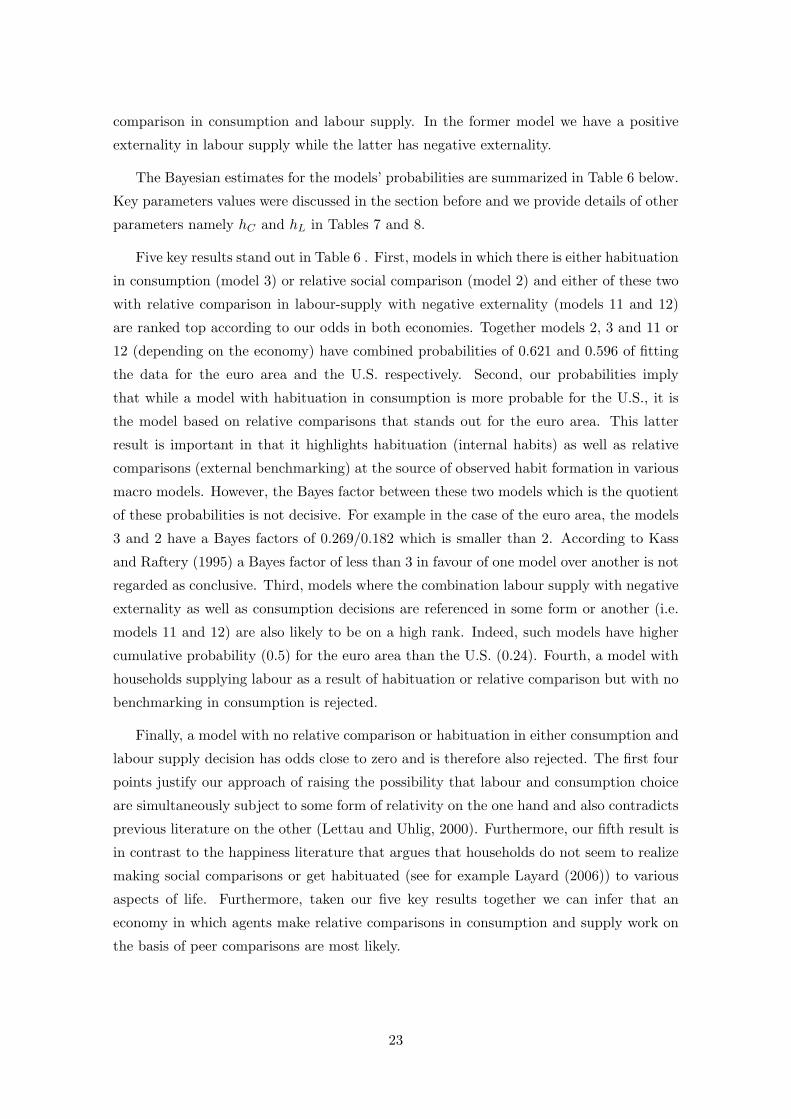
Five key results stand out in Table 6 . First, models in which there is either habituation

in consumption (model 3) or relative social comparison (model 2) and either of these two

with relative comparison in labour-supply with negative externality (models 11 and 12)

are ranked top according to our odds in both economies. Together models 2, 3 and 11 or

12 (depending on the economy) have combined probabilities of 0.621 and 0.596 of fitting

the data for the euro area and the U.S. respectively. Second, our probabilities imply

that while a model with habituation in consumption is more probable for the U.S., it is

the model based on relative comparisons that stands out for the euro area. This latter

result is important in that it highlights habituation (internal habits) as well as relative

comparisons (external benchmarking) at the source of observed habit formation in various

macro models. However, the Bayes factor between these two models which is the quotient

of these probabilities is not decisive. For example in the case of the euro area, the models

3 and 2 have a Bayes factors of 0.269/0.182 which is smaller than 2. According to Kass

and Raftery (1995) a Bayes factor of less than 3 in favour of one model over another is not

regarded as conclusive. Third, models where the combination labour supply with negative

externality as well as consumption decisions are referenced in some form or another (i.e.

models 11 and 12) are also likely to be on a high rank. Indeed, such models have higher

cumulative probability (0.5) for the euro area than the U.S. (0.24). Fourth, a model with

households supplying labour as a result of habituation or relative comparison but with no

benchmarking in consumption is rejected.

Finally, a model with no relative comparison or habituation in either consumption and

labour supply decision has odds close to zero and is therefore also rejected. The first four

points justify our approach of raising the possibility that labour and consumption choice

are simultaneously subject to some form of relativity on the one hand and also contradicts

previous literature on the other (Lettau and Uhlig, 2000). Furthermore, our fifth result is

in contrast to the happiness literature that argues that households do not seem to realize

making social comparisons or get habituated (see for example Layard (2006)) to various

aspects of life. Furthermore, taken our five key results together we can infer that an

economy in which agents make relative comparisons in consumption and supply work on

the basis of peer comparisons are most likely.

23

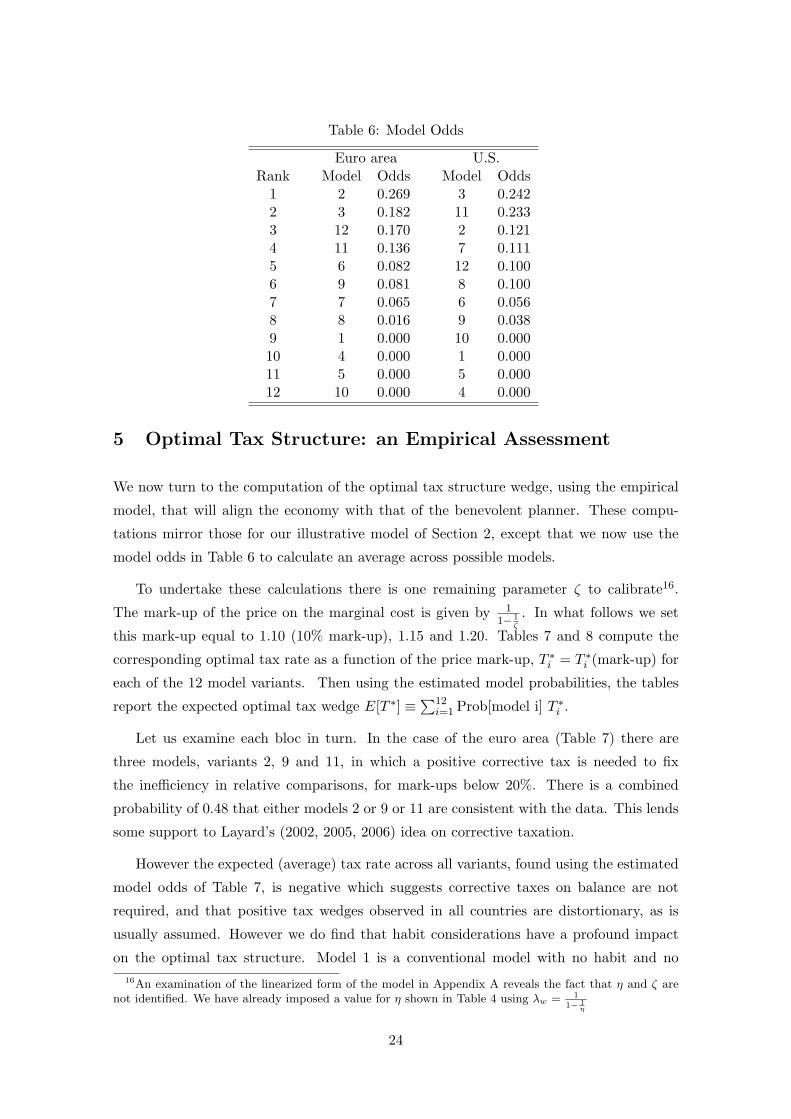
Table 6: Model Odds

Euro area U.S.Rank Model Odds Model Odds

1 2 0.269 3 0.2422 3 0.182 11 0.2333 12 0.170 2 0.1214 11 0.136 7 0.1115 6 0.082 12 0.1006 9 0.081 8 0.1007 7 0.065 6 0.0568 8 0.016 9 0.0389 1 0.000 10 0.00010 4 0.000 1 0.00011 5 0.000 5 0.00012 10 0.000 4 0.000

5 Optimal Tax Structure: an Empirical Assessment

We now turn to the computation of the optimal tax structure wedge, using the empirical

model, that will align the economy with that of the benevolent planner. These compu-

tations mirror those for our illustrative model of Section 2, except that we now use the

model odds in Table 6 to calculate an average across possible models.

To undertake these calculations there is one remaining parameter ζ to calibrate16.

The mark-up of the price on the marginal cost is given by 11− 1

ζ

. In what follows we set

this mark-up equal to 1.10 (10% mark-up), 1.15 and 1.20. Tables 7 and 8 compute the

corresponding optimal tax rate as a function of the price mark-up, T ∗i = T ∗i (mark-up) for

each of the 12 model variants. Then using the estimated model probabilities, the tables

report the expected optimal tax wedge E[T ∗] ≡∑12

i=1 Prob[model i] T ∗i .

Let us examine each bloc in turn. In the case of the euro area (Table 7) there are

three models, variants 2, 9 and 11, in which a positive corrective tax is needed to fix

the inefficiency in relative comparisons, for mark-ups below 20%. There is a combined

probability of 0.48 that either models 2 or 9 or 11 are consistent with the data. This lends

some support to Layard’s (2002, 2005, 2006) idea on corrective taxation.

However the expected (average) tax rate across all variants, found using the estimated

model odds of Table 7, is negative which suggests corrective taxes on balance are not

required, and that positive tax wedges observed in all countries are distortionary, as is

usually assumed. However we do find that habit considerations have a profound impact

on the optimal tax structure. Model 1 is a conventional model with no habit and no16An examination of the linearized form of the model in Appendix A reveals the fact that η and ζ are

not identified. We have already imposed a value for η shown in Table 4 using λw = 1

1− 1η

24

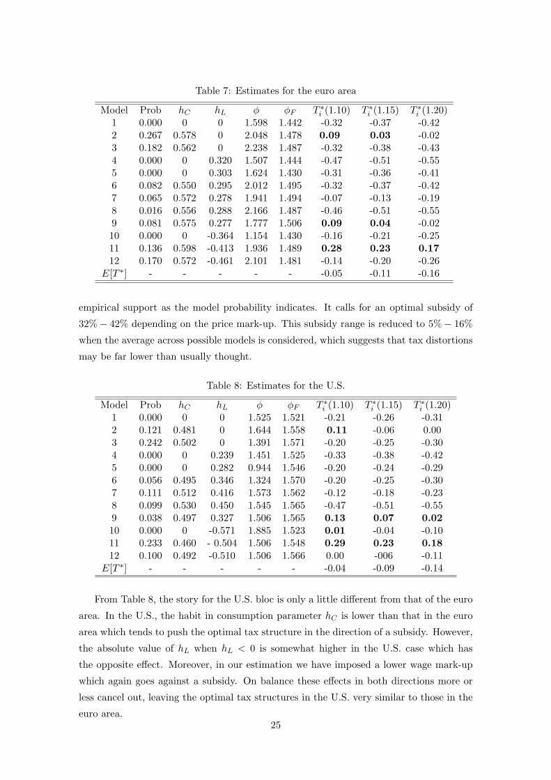
Table 7: Estimates for the euro area

Model Prob hC hL φ φF T ∗i (1.10) T ∗i (1.15) T ∗i (1.20)1 0.000 0 0 1.598 1.442 -0.32 -0.37 -0.422 0.267 0.578 0 2.048 1.478 0.09 0.03 -0.023 0.182 0.562 0 2.238 1.487 -0.32 -0.38 -0.434 0.000 0 0.320 1.507 1.444 -0.47 -0.51 -0.555 0.000 0 0.303 1.624 1.430 -0.31 -0.36 -0.416 0.082 0.550 0.295 2.012 1.495 -0.32 -0.37 -0.427 0.065 0.572 0.278 1.941 1.494 -0.07 -0.13 -0.198 0.016 0.556 0.288 2.166 1.487 -0.46 -0.51 -0.559 0.081 0.575 0.277 1.777 1.506 0.09 0.04 -0.0210 0.000 0 -0.364 1.154 1.430 -0.16 -0.21 -0.2511 0.136 0.598 -0.413 1.936 1.489 0.28 0.23 0.1712 0.170 0.572 -0.461 2.101 1.481 -0.14 -0.20 -0.26

E[T ∗] - - - - - -0.05 -0.11 -0.16

empirical support as the model probability indicates. It calls for an optimal subsidy of

32%− 42% depending on the price mark-up. This subsidy range is reduced to 5%− 16%

when the average across possible models is considered, which suggests that tax distortions

may be far lower than usually thought.

Table 8: Estimates for the U.S.

Model Prob hC hL φ φF T ∗i (1.10) T ∗i (1.15) T ∗i (1.20)1 0.000 0 0 1.525 1.521 -0.21 -0.26 -0.312 0.121 0.481 0 1.644 1.558 0.11 -0.06 0.003 0.242 0.502 0 1.391 1.571 -0.20 -0.25 -0.304 0.000 0 0.239 1.451 1.525 -0.33 -0.38 -0.425 0.000 0 0.282 0.944 1.546 -0.20 -0.24 -0.296 0.056 0.495 0.346 1.324 1.570 -0.20 -0.25 -0.307 0.111 0.512 0.416 1.573 1.562 -0.12 -0.18 -0.238 0.099 0.530 0.450 1.545 1.565 -0.47 -0.51 -0.559 0.038 0.497 0.327 1.506 1.565 0.13 0.07 0.0210 0.000 0 -0.571 1.885 1.523 0.01 -0.04 -0.1011 0.233 0.460 - 0.504 1.506 1.548 0.29 0.23 0.1812 0.100 0.492 -0.510 1.506 1.566 0.00 -006 -0.11

E[T ∗] - - - - - -0.04 -0.09 -0.14

From Table 8, the story for the U.S. bloc is only a little different from that of the euro

area. In the U.S., the habit in consumption parameter hC is lower than that in the euro

area which tends to push the optimal tax structure in the direction of a subsidy. However,

the absolute value of hL when hL < 0 is somewhat higher in the U.S. case which has

the opposite effect. Moreover, in our estimation we have imposed a lower wage mark-up

which again goes against a subsidy. On balance these effects in both directions more or

less cancel out, leaving the optimal tax structures in the U.S. very similar to those in the

euro area.25

6 Conclusion

In this paper we use a dynamic general-equilibrium model to study happiness theoretically

and empirically. In particular, following on from the happiness literature, we examine the

role of relative preferences, that affect the choices of consumption and labour supply,

play in explaining the ‘happiness inertia.’ Our theoretical implies that habits and social

comparison in consumption and labour supply can only provide a partial explanation to

the problem of ‘happiness inertia.’ Bayesian estimations of our models empirically support

the ideas of habituation and relative comparison in consumption and peer comparison in

labour supply. Generally, our results find little empirical support for taxation as a method

for mitigating the inefficiencies that exist in our models. Indeed, in most cases of our

estimations the optimal tax wedge is negative implying a distortionary and not corrective

effect of taxation. However it is still the case that the presence of social comparisons

means taxes are less distortionary than otherwise. There is one exception however. A

model in which households make social comparisons and face peer pressure at work was

found to have relatively high probability to match the data with a positive tax policy

recommendation. On average, though, taxes are found to be (slightly) distortionary and

in fact add to the inefficiencies that reduce output and work effort below that of the social

planner.

26

References

Adolfson, M., Lasseen, S., Linde, J., and Villani, M. (2005). The role of sticky pricesin an open economy DSGE model: a Bayesian investigation. Journal of the EuropeanEconomic Association, 3(2-3):444–457.

Adolfson, M., Lasseen, S., Linde, J., and Villani, M. (2007). Bayesian estimation of anopen economy DSGE model with incomplete pass-through. Journal of InternationalEconomics (forthcoming).

An, S. and Schorfheide, F. (2007). Bayesian analysis of DSGE models. EconometricReviews, 26(2-4):113–172.

Arrow, K. J. and Dasgupta, P. (2007). Conspicuous consumption, inconspicuous leisure.Paper prepared for the James Meade Centenary meeting, July 12-13, 2007, Bank ofEngland.

Blanchard, O. J. (2004). The economic future of Europe. Journal of Economic Perspec-tives, 18:3–26.

Blanchflower, D. G. and Oswald, A. J. (2000). Well-being over time in Britain and theUSA. NBER Working Paper No. 7487.

Calvo, G. (1983). Staggered prices in a utility maximising framework. Journal of MonetaryEconomics, 12(3):383–398.

Canova, F. and Ortega, E. (2000). Testing calibrated general equilibrium models. InMariano, R., Schuerman, T., and Weeks, M., editors, Simulation-based Inference inEconometrics: Methods and Applications. Cambridge University Press.

Choudhary, A. M. and Levine, P. (2006). Idle worship. Economics Letters, 90(1):77–83.

Christiano, L., Eichenbaum, M., and Evans, C. (2005). Nominal rigidities and the dynamiceffects of a shock to monetary policy. Journal of Political Economy, 118(1):1–45.

Christiano, L. and Haan, W. D. (1996). Small sample properties of GMM for businesscycle analysis. Journal of Business and Economic Statistics, 14(3):309–327.

Clark, A. (1999). Are wages habit forming, evidence from micro data. Journal of EconomicBehaviour and Organisation, 39(2):179–200.

Clark, A. and Oswald, A. J. (1996). Satisfaction and comparison income. Journal ofPublic Economics, 61(3):359–381.

Coenen, G., McAdam, P., and Straub, R. (2007). Tax reform and labour-market perfor-mance in the euro area: a simulation-based analysis using the New Area Wide Model.Journal of Economic Dynamics and Control.

DeJong, D., Ingram, B., and Whiteman, C. (2000a). A Bayesian approach to dynamicmacroeconomics. Journal of Econometrics, 98(2):203–223.

DeJong, D., Ingram, B., and Whiteman, C. (2000b). Keynesian impulses versus Solowresiduals: identifying sources of business cycle fluctuations. Journal of Applied Econo-metrics, 15(3):311–329.

27

Di Tella, R., MacCulloch, R., and Oswald, A. J. (2003). The macroeconomics of happiness.Review of Economics and Statistics, 85(4):793–809.

Easterlin, R. A. (1974). Does economic growth improve the human lot? some evidence. InDavid, P. A. and Reder, M. W., editors, Nations and Households in Economic Growth:Essays in Honor of Moses Abramowitz. New York Academic Press.

Fagan, G., Henry, J., and Mestre, R. (2001). An area-wide model AWM of the euro area.Working Paper No. 42, European Central Bank.

Favero, C. (2001). Applied Macroeconometrics. Oxford University Press.

Frey, B. S. and Stutzer, A. (2001). Happiness and Economics: How the Economy andInstitutions Affect Human Well-Being. Princeton University Press.

Galı, J. and Gertler, M. (1999). Inflation dynamics: a structural econometric analysis.Journal of Monetary Economics, 44(2):195–222.

Geweke, J. (1999). Using simulation methods for Bayesian econometric models: inference,development and communication. Econometric Reviews, 18(1):1–126.

Harvey, A. C. (1989). Forecasting, Structural Time Series Models and the Kalman Filter.Cambridge University Press.

Justiniano, A. and Preston, B. (2004). Small open economy DSGE models: specification,estimation and model fit. Manuscript IMF.

Kahneman, D., Diener, E., and Schwarz, N. (1999). Well-Being: The Foundations ofHedonic Pshchology. Russell Sage Foundation, New York.

Kass, R. E. and Raftery, A. E. (1995). Bayes factors. Journal of the American StatisticalAssociation, 90(430):773–795.

Kim, J. (2000). Constructing and estimating a realistic optimising model of monetarypolicy. Journal of Monetary Economics, 45(2):329–360.

Kim, K. and Pagan, A. (1994). The econometric analysis of calibrated macroeconomicmodels. In Pesaran, H. and Wickens, M., editors, Handbook of Applied Econometrics,volume 1. Blackwell Press, London.

Layard, R. (2002). Rethinking public economics: the implication of rivalry and habit.Mimeo, Centre for Economic Performance, London School of Economics.

Layard, R. (2005). Happiness: Lessons from a New Science. Penguin, New York andLondon.

Layard, R. (2006). Happiness and public policy: a challenge to the profession. EconomicJournal, 116(510):C24–C33.

Leeper, E. and Sims, C. A. (1994). Towars a modern macroeconomic model usable forpolicy analysis. NBER Macroeconomics Annual, pages 81–118.

Lettau, M. and Uhlig, H. (2000). Can habit formation be reconciled with business cyclefacts? Review of Economic Dynamics, 3(1):79–99.

28

Levin, A. T., Onatski, A., Williams, J. C., and Williams, N. (2005). Monetary policyunder uncertainty in micro-founded macroeconometric models. NBER MacroeconomicsAnnual.

Lubik, T. A. and Schorfheide, F. (2004). Testing for indeterminacy: an application toU.S. monetary policy. American Economic Review, 94(1):190–217.

McGrattan, E. R. (1994). The macroeconomic effects of distortionary taxation. Journalof Monetary Economics, 33(3):573–601.

Oates, W. E. (1971). Confessions of a Workaholic: The Facts about Work Addiction.World, New York.

Otrok, C. (2001). On measuring the welfare cost of business cycles. Journal of MonetaryEconomics, 47(1):61–92.

Prescott, E. C. (2004). Why do Americans work so much more than Europeans? FedrealReserve Bank of Minneapolis Quarterly Review, 28:2–13.

Rabanal, P. and Rubio-Ramırez, J. F. (2005). Comparing new Keynesian models of thebusiness cycle: a Bayesian approach. Journal of Monetary Economics, 52(6):1151–1166.

Rayo, L. and Becker, G. S. (2007). Evolutionary efficiency and happiness. Journal ofPolitical Economy, 115(2):302–337.

Sargent, T. (1989). Two models of measurements and the investment accelerator. Journalof Political Economy, 97(2):251–287.

Smets, F. and Wouters, R. (2003). An estimated dynamic stochastic general equilibriummodel of the euro area. Journal of the European Economic Association, 1(5):1123–1175.

Stutzer, A. (2004). The role of income aspirations in individual happiness. Journal ofEconomic Behaviour and Organization, 54(1):89–109.

Van Praag, B. M. and Frijters, P. (1999). The measurement of welfare and well-being:the leyden approach. In Kahneman, D., Diener, E., and Schwarz, N., editors, TheFoundations of Hedonic Psychology. Russell Sage Foundation, New York.

29

Appendices

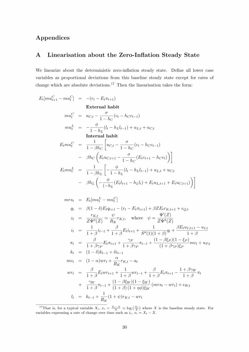
A Linearisation about the Zero-Inflation Steady State

We linearize about the deterministic zero-inflation steady state. Define all lower case

variables as proportional deviations from this baseline steady state except for rates of

change which are absolute deviations.17 Then the linearisation takes the form:

Et[muCt+1 −muCt ] = −(rt − Etπt+1)

External habit

muCt = uC,t −σ

1− hC(ct − hCct−1)

muLt = − φ

1− hL(lt − hLlt−1) + uL,t + uC,t

Internal habit

EtmuCt =

11− βhC

[uC,t −

σ

1− hC(ct − hCct−1)

− βhC

(EtuC,t+1 −

σ

1− hC(Etct+1 − hCct)

)]Etmu

Lt =

11− βhL

[− φ

1− hL(lt − hLlt−1) + uL,t + uC,t

− βhL

(− φ

(−hL(Etlt+1 − hLlt) + EtuL,t+1 + EtuC,t+1)

)]

mrst = Et[muLt −muCt ]

qt = β(1− δ)Etqt+1 − (rt − Etπt+1) + βZEtrK,t+1 + εQ,t

zt =rK,t

ZΨ′′(Z)=

ψ

RKrK,t, where ψ =

Ψ′(Z)ZΨ′′(Z)

it =1

1 + βit−1 +

β

1 + βEtit+1 +

1S′′(1)(1 + β)

qt +βEtuI,t+1 − uI,t

1 + β

πt =β

1 + βγPEtπt+1 +

γP1 + βγP

πt−1 +(1− βξP )(1− ξP )

(1 + βγP )ξPmct + uP,t

kt = (1− δ)kt−1 + δit−1

mct = (1− α)wrt +α

RKrK,t − at

wrt =β

1 + βEtwrt+1 +

11 + β

wrt−1 +β

1 + βEtπt+1 −

1 + βγW1 + β

πt

+γW

1 + βπt−1 +

(1− βξW )(1− ξW )(1 + β) (1 + ηφ)ξW

(mrst − wrt) + εW,t

lt = kt−1 +1RK

(1 + ψ)rK,t − wrt

17That is, for a typical variable Xt, xt = Xt−XX

' log(XtX

)where X is the baseline steady state. For

variables expressing a rate of change over time such as it, xt = Xt −X.

30

yt = cyct + gygt + iyit + kyψrK,t

yt = φF

[at + α(

ψ

RKrK,t + kt−1) + (1− α)lt

], where φF = 1 +

F

Y

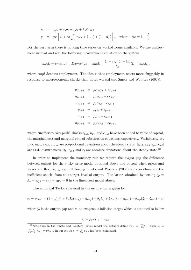
For the euro area there is no long time series on worked hours available. We use employ-

ment instead and add the following measurement equation to the system

emplt = emplt−1 + Etemplt+1 − emplt +(1− βξe)(1− ξe)

ξe(lt − emplt),

where empl denotes employment. The idea is that employment reacts more sluggishly in

response to macroeconomic shocks than hours worked (see Smets and Wouters (2003)).

uC,t+1 = ρCuC,t + εC,t+1

uL,t+1 = ρLuL,t + εL,t+1

uI,t+1 = ρIuI,t + εI,t+1

gt+1 = ρggt + εg,t+1

at+1 = ρaat + εa,t+1

uP,t+1 = ρPuP,t + εP,t+1

where “inefficient cost-push” shocks εQ,t, uP,t and εW,t have been added to value of capital,

the marginal cost and marginal rate of substitution equations respectively. Variables yt, ct,

mct, uC,t, uN,t, at, gt are proportional deviations about the steady state. [εC,t, εN,t, εg,t, εa,t]

are i.i.d. disturbances. πt, rK,t and rt are absolute deviations about the steady state.18

In order to implement the monetary rule we require the output gap the difference

between output for the sticky price model obtained above and output when prices and

wages are flexible, yt say. Following Smets and Wouters (2003) we also eliminate the

inefficient shocks from this target level of output. The latter, obtained by setting ξp =

ξw = εQ,t = εP,t = εW,t = 0 in the linearized model above.

The empirical Taylor rule used in the estimation is given by

rt = ρrt−1 + (1− ρ)[πt + θπEt(πt+j − πt+j) + θyyt] + θ∆π(πt − πt−1) + θ∆y(yt − yt−1) + εt

where yt is the output gap and πt an exogenous inflation target which is assumed to follow

πt = ρππt−1 + επ,t.

18Note that in the Smets and Wouters (2003) model the authors define rK,t =rK,tRK

. Then zt =Ψ′(Z)ZΨ′′(Z)

rK,t = ψrK,t. In our set-up zt = ψRK

rK,t has been eliminated.

31

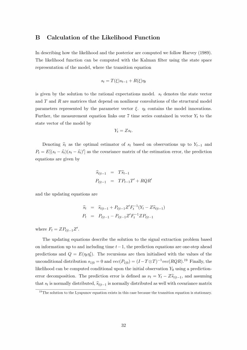
B Calculation of the Likelihood Function

In describing how the likelihood and the posterior are computed we follow Harvey (1989).

The likelihood function can be computed with the Kalman filter using the state space

representation of the model, where the transition equation

st = T (ξ)st−1 +R(ξ)ηt

is given by the solution to the rational expectations model. st denotes the state vector

and T and R are matrices that depend on nonlinear convolutions of the structural model

parameters represented by the parameter vector ξ. ηt contains the model innovations.

Further, the measurement equation links our 7 time series contained in vector Yt to the

state vector of the model by

Yt = Zst.

Denoting st as the optimal estimator of st based on observations up to Yt−1 and

Pt = E[(st − st)(st − st)′] as the covariance matrix of the estimation error, the prediction

equations are given by

st|t−1 = T st−1

Pt|t−1 = TPt−1T′ +RQR′

and the updating equations are

st = st|t−1 + Pt|t−1Z′F−1t (Yt − Zst|t−1)

Pt = Pt|t−1 − Pt|t−1Z′F−1t ZPt|t−1

where Ft = ZPt|t−1Z′.

The updating equations describe the solution to the signal extraction problem based

on information up to and including time t−1, the prediction equations are one-step ahead

predictions and Q = E(ηtη′t). The recursions are then initialised with the values of the

unconditional distribution s1|0 = 0 and vec(P1|0) = (I−T⊗T )−1vec(RQR).19 Finally, the

likelihood can be computed conditional upon the initial observation Y0 using a prediction-

error decomposition. The prediction error is defined as νt = Yt − Zst|t−1, and assuming

that st is normally distributed, st|t−1 is normally distributed as well with covariance matrix

19The solution to the Lyapunov equation exists in this case because the transition equation is stationary.

32

Pt|t−1. It follows that the log-likelihood can be written as

logL(Y |ξ) = −12

NT log 2π −

T∑t=1

log |Ft| −T∑t=1

ν ′tF−1t νt

.

Computation of the log-posterior distribution ϕ(ξ|Y ) requires calculating the log-likelihood

and then adding the log-prior density evaluated at ξ. The likelihood itself is computed

by applying the Kalman filter recursions to the above state space system after solving the

model given values of the elements in the parameter vector ξ.

33

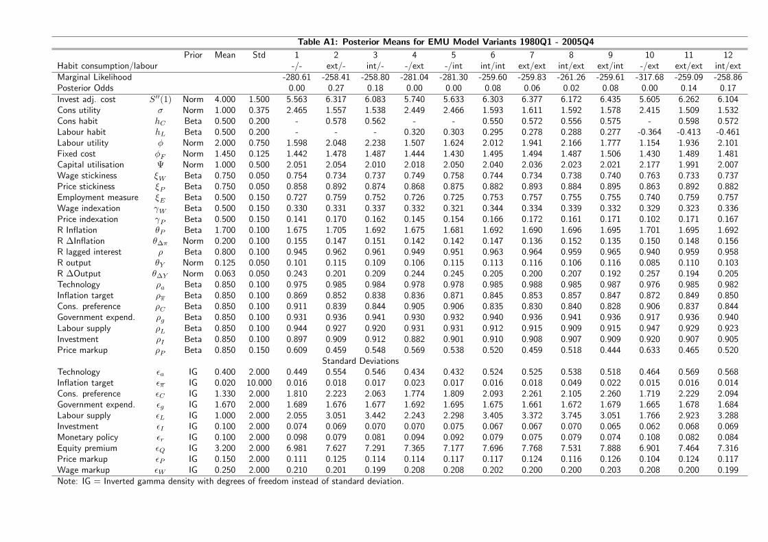
Table A1: Posterior Means for EMU Model Variants 1980Q1 - 2005Q4Prior Mean Std 1 2 3 4 5 6 7 8 9 10 11 12

Habit consumption/labour -/- ext/- int/- -/ext -/int int/int ext/ext int/ext ext/int -/ext ext/ext int/extMarginal Likelihood -280.61 -258.41 -258.80 -281.04 -281.30 -259.60 -259.83 -261.26 -259.61 -317.68 -259.09 -258.86Posterior Odds 0.00 0.27 0.18 0.00 0.00 0.08 0.06 0.02 0.08 0.00 0.14 0.17Invest adj. cost S00(1) Norm 4.000 1.500 5.563 6.317 6.083 5.740 5.633 6.303 6.377 6.172 6.435 5.605 6.262 6.104Cons utility Norm 1.000 0.375 2.465 1.557 1.538 2.449 2.466 1.593 1.611 1.592 1.578 2.415 1.509 1.532Cons habit hC Beta 0.500 0.200 - 0.578 0.562 - - 0.550 0.572 0.556 0.575 - 0.598 0.572Labour habit hL Beta 0.500 0.200 - - - 0.320 0.303 0.295 0.278 0.288 0.277 -0.364 -0.413 -0.461Labour utility Norm 2.000 0.750 1.598 2.048 2.238 1.507 1.624 2.012 1.941 2.166 1.777 1.154 1.936 2.101Fixed cost F Norm 1.450 0.125 1.442 1.478 1.487 1.444 1.430 1.495 1.494 1.487 1.506 1.430 1.489 1.481Capital utilisation Norm 1.000 0.500 2.051 2.054 2.010 2.018 2.050 2.040 2.036 2.023 2.021 2.177 1.991 2.007Wage stickiness W Beta 0.750 0.050 0.754 0.734 0.737 0.749 0.758 0.744 0.734 0.738 0.740 0.763 0.733 0.737Price stickiness P Beta 0.750 0.050 0.858 0.892 0.874 0.868 0.875 0.882 0.893 0.884 0.895 0.863 0.892 0.882Employment measure E Beta 0.500 0.150 0.727 0.759 0.752 0.726 0.725 0.753 0.757 0.755 0.755 0.740 0.759 0.757Wage indexation W Beta 0.500 0.150 0.330 0.331 0.337 0.332 0.321 0.344 0.334 0.339 0.332 0.329 0.323 0.336Price indexation P Beta 0.500 0.150 0.141 0.170 0.162 0.145 0.154 0.166 0.172 0.161 0.171 0.102 0.171 0.167R Ination P Beta 1.700 0.100 1.675 1.705 1.692 1.675 1.681 1.692 1.690 1.696 1.695 1.701 1.695 1.692R Ination Norm 0.200 0.100 0.155 0.147 0.151 0.142 0.142 0.147 0.136 0.152 0.135 0.150 0.148 0.156R lagged interest Beta 0.800 0.100 0.945 0.962 0.961 0.949 0.951 0.963 0.964 0.959 0.965 0.940 0.959 0.958R output Y Norm 0.125 0.050 0.101 0.115 0.109 0.106 0.115 0.113 0.116 0.106 0.116 0.085 0.110 0.103R Output Y Norm 0.063 0.050 0.243 0.201 0.209 0.244 0.245 0.205 0.200 0.207 0.192 0.257 0.194 0.205Technology a Beta 0.850 0.100 0.975 0.985 0.984 0.978 0.978 0.985 0.988 0.985 0.987 0.976 0.985 0.982Ination target Beta 0.850 0.100 0.869 0.852 0.838 0.836 0.871 0.845 0.853 0.857 0.847 0.872 0.849 0.850Cons. preference C Beta 0.850 0.100 0.911 0.839 0.844 0.905 0.906 0.835 0.830 0.840 0.828 0.906 0.837 0.844Government expend. g Beta 0.850 0.100 0.931 0.936 0.941 0.930 0.932 0.940 0.936 0.941 0.936 0.917 0.936 0.940Labour supply L Beta 0.850 0.100 0.944 0.927 0.920 0.931 0.931 0.912 0.915 0.909 0.915 0.947 0.929 0.923Investment I Beta 0.850 0.100 0.897 0.909 0.912 0.882 0.901 0.910 0.908 0.907 0.909 0.920 0.907 0.905Price markup P Beta 0.850 0.150 0.609 0.459 0.548 0.569 0.538 0.520 0.459 0.518 0.444 0.633 0.465 0.520

Standard DeviationsTechnology a IG 0.400 2.000 0.449 0.554 0.546 0.434 0.432 0.524 0.525 0.538 0.518 0.464 0.569 0.568Ination target IG 0.020 10.000 0.016 0.018 0.017 0.023 0.017 0.016 0.018 0.049 0.022 0.015 0.016 0.014Cons. preference C IG 1.330 2.000 1.810 2.223 2.063 1.774 1.809 2.093 2.261 2.105 2.260 1.719 2.229 2.094Government expend. g IG 1.670 2.000 1.689 1.676 1.677 1.692 1.695 1.675 1.661 1.672 1.679 1.665 1.678 1.684Labour supply L IG 1.000 2.000 2.055 3.051 3.442 2.243 2.298 3.405 3.372 3.745 3.051 1.766 2.923 3.288Investment I IG 0.100 2.000 0.074 0.069 0.070 0.070 0.075 0.067 0.067 0.070 0.065 0.062 0.068 0.069Monetary policy r IG 0.100 2.000 0.098 0.079 0.081 0.094 0.092 0.079 0.075 0.079 0.074 0.108 0.082 0.084Equity premium Q IG 3.200 2.000 6.981 7.627 7.291 7.365 7.177 7.696 7.768 7.531 7.888 6.901 7.464 7.316Price markup P IG 0.150 2.000 0.111 0.125 0.114 0.114 0.117 0.117 0.124 0.116 0.126 0.104 0.124 0.117Wage markup W IG 0.250 2.000 0.210 0.201 0.199 0.208 0.208 0.202 0.200 0.200 0.203 0.208 0.200 0.199Note: IG = Inverted gamma density with degrees of freedom instead of standard deviation.

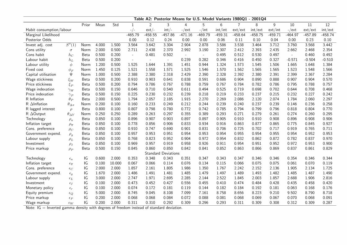
Table A2: Posterior Means for U.S. Model Variants 1980Q1 - 2001Q4Prior Mean Std 1 2 3 4 5 6 7 8 9 10 11 12

Habit consumption/labour -/- ext/- int/- -/ext -/int int/int ext/ext int/ext ext/int -/ext ext/ext int/extMarginal Likelihood -465.79 -458.55 -457.86 -471.16 -469.79 -459.31 -458.64 -458.75 -459.71 -464.97 -457.89 -458.74Posterior Odds 0.00 0.12 0.24 0.00 0.00 0.06 0.11 0.10 0.04 0.00 0.23 0.10Invest adj. cost S00(1) Norm 4.000 1.500 3.564 3.642 3.304 2.904 2.878 3.586 3.538 3.464 3.712 3.760 3.568 3.442Cons utility Norm 2.000 0.500 2.711 2.438 2.370 2.992 3.190 2.307 2.412 2.393 2.435 2.662 2.468 2.354Cons habit hC Beta 0.500 0.200 - 0.481 0.502 - - 0.495 0.512 0.530 0.497 - 0.460 0.492Labour habit hL Beta 0.500 0.200 - - - 0.239 0.282 0.346 0.416 0.450 0.327 -0.571 -0.504 -0.510Labour utility Norm 1.200 0.500 1.525 1.644 1.391 1.451 0.944 1.324 1.573 1.545 1.506 1.665 1.648 1.384Fixed cost F Norm 1.450 0.125 1.521 1.558 1.571 1.525 1.546 1.570 1.562 1.565 1.565 1.523 1.548 1.566Capital utilisation Norm 1.000 0.500 2.388 2.380 2.318 2.429 2.390 2.328 2.392 2.380 2.391 2.399 2.367 2.284Wage stickiness W Beta 0.500 0.200 0.910 0.903 0.641 0.838 0.591 0.686 0.904 0.890 0.888 0.907 0.904 0.570Price stickiness P Beta 0.500 0.200 0.794 0.786 0.767 0.788 0.759 0.767 0.784 0.782 0.786 0.795 0.788 0.757Wage indexation W Beta 0.500 0.150 0.646 0.710 0.540 0.611 0.494 0.525 0.719 0.698 0.702 0.644 0.708 0.468Price indexation P Beta 0.500 0.150 0.225 0.230 0.232 0.239 0.218 0.219 0.233 0.237 0.215 0.232 0.227 0.242R Ination P Beta 2.000 0.500 1.794 2.057 2.185 1.915 2.270 2.269 2.086 2.120 2.074 1.784 2.060 2.297R Ination Norm 0.200 0.100 0.160 0.233 0.249 0.212 0.244 0.239 0.240 0.237 0.239 0.146 0.236 0.258R lagged interest Beta 0.800 0.100 0.807 0.798 0.780 0.772 0.742 0.785 0.794 0.799 0.796 0.818 0.804 0.770R Output Y Norm 0.250 0.250 0.289 0.263 0.297 0.355 0.389 0.293 0.271 0.279 0.261 0.274 0.260 0.295Technology a Beta 0.850 0.100 0.896 0.907 0.903 0.897 0.897 0.905 0.910 0.910 0.908 0.896 0.908 0.906Ination target Beta 0.850 0.100 0.778 0.856 0.906 0.833 0.934 0.916 0.863 0.877 0.865 0.775 0.845 0.927Cons. preference C Beta 0.850 0.100 0.910 0.747 0.690 0.901 0.831 0.706 0.725 0.702 0.717 0.919 0.765 0.711Government expend. g Beta 0.850 0.100 0.957 0.953 0.951 0.954 0.953 0.954 0.955 0.954 0.955 0.954 0.952 0.953Labour supply L Beta 0.850 0.100 0.768 0.823 0.952 0.904 0.972 0.954 0.832 0.862 0.872 0.782 0.837 0.970Investment I Beta 0.850 0.100 0.969 0.957 0.919 0.958 0.926 0.911 0.954 0.951 0.952 0.972 0.953 0.900Price markup P Beta 0.500 0.150 0.845 0.860 0.850 0.842 0.841 0.852 0.863 0.866 0.869 0.837 0.861 0.829

Standard DeviationsTechnology a IG 0.600 2.000 0.353 0.348 0.343 0.351 0.347 0.343 0.347 0.346 0.346 0.354 0.346 0.344Ination target IG 0.100 10.000 0.067 0.066 0.114 0.076 0.134 0.115 0.066 0.075 0.075 0.061 0.070 0.119Cons. preference C IG 2.000 2.000 1.857 2.161 1.805 1.986 1.350 1.767 2.242 2.152 2.136 1.905 2.134 1.725Government expend. g IG 1.670 2.000 1.486 1.491 1.481 1.485 1.479 1.497 1.489 1.493 1.482 1.485 1.487 1.490Labour supply L IG 3.000 2.000 2.747 1.971 2.695 2.285 2.144 2.522 1.845 2.003 1.857 2.688 1.906 2.816Investment I IG 0.100 2.000 0.473 0.452 0.427 0.556 0.455 0.410 0.474 0.484 0.428 0.435 0.458 0.420Monetary policy r IG 0.100 2.000 0.074 0.172 0.181 0.119 0.144 0.182 0.184 0.192 0.181 0.063 0.168 0.176Equity premium Q IG 5.000 2.000 8.745 9.045 8.108 7.099 7.161 8.758 8.656 8.223 9.210 9.502 8.790 8.718Price markup P IG 0.200 2.000 0.068 0.068 0.084 0.072 0.088 0.081 0.068 0.069 0.067 0.070 0.068 0.091Wage markup W IG 0.200 2.000 0.311 0.310 0.292 0.309 0.296 0.293 0.311 0.309 0.308 0.312 0.309 0.287Note: IG = Inverted gamma density with degrees of freedom instead of standard deviation.

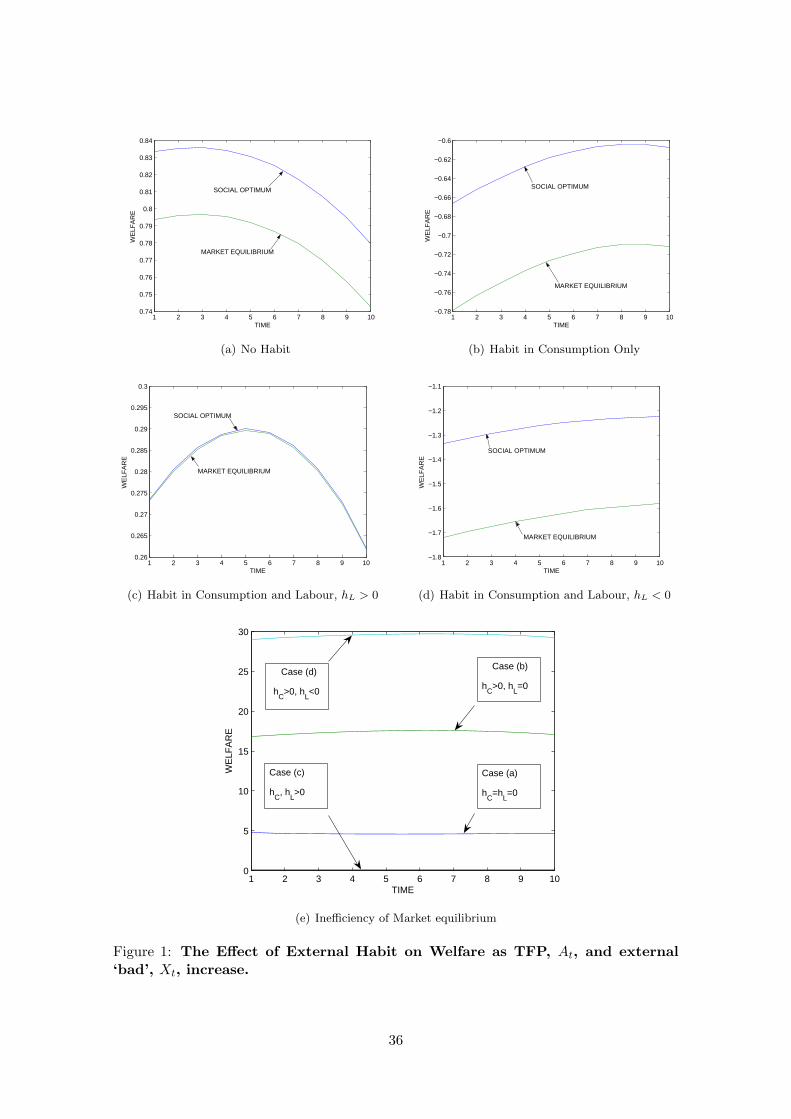
1 2 3 4 5 6 7 8 9 100.74

0.75

0.76

0.77

0.78

0.79

0.8

0.81

0.82

0.83

0.84

TIME

WE

LFA

RE

MARKET EQUILIBRIUM

SOCIAL OPTIMUM

(a) No Habit

1 2 3 4 5 6 7 8 9 10−0.78

−0.76

−0.74

−0.72

−0.7

−0.68

−0.66

−0.64

−0.62

−0.6

TIME

WE

LFA

RE

SOCIAL OPTIMUM

MARKET EQUILIBRIUM

(b) Habit in Consumption Only

1 2 3 4 5 6 7 8 9 100.26

0.265

0.27

0.275

0.28

0.285

0.29

0.295

0.3

TIME

WE

LFA

RE

MARKET EQUILIBRIUM

SOCIAL OPTIMUM

(c) Habit in Consumption and Labour, hL > 0

1 2 3 4 5 6 7 8 9 10−1.8

−1.7

−1.6

−1.5

−1.4

−1.3

−1.2

−1.1

TIME

WE

LFA

RE

MARKET EQUILIBRIUM

SOCIAL OPTIMUM

(d) Habit in Consumption and Labour, hL < 0

1 2 3 4 5 6 7 8 9 100

5

10

15

20

25

30

TIME

WE

LFA

RE

Case (b)

hC

>0, hL=0

Case (a)

hC

=hL=0

Case (d)

hC

>0, hL<0

Case (c)

hC

, hL>0

(e) Inefficiency of Market equilibrium

Figure 1: The Effect of External Habit on Welfare as TFP, At, and external‘bad’, Xt, increase.

36

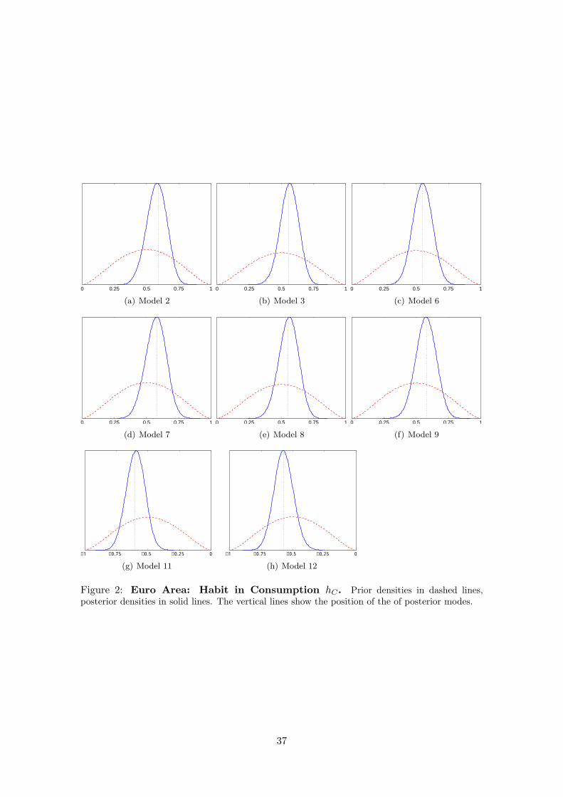
0 0.25 0.5 0.75 1

(a) Model 2

0 0.25 0.5 0.75 1

(b) Model 3

0 0.25 0.5 0.75 1

(c) Model 6

0 0.25 0.5 0.75 1

(d) Model 7

0 0.25 0.5 0.75 1

(e) Model 8

0 0.25 0.5 0.75 1

(f) Model 9

−1 −0.75 −0.5 −0.25 0

(g) Model 11

−1 −0.75 −0.5 −0.25 0

(h) Model 12

Figure 2: Euro Area: Habit in Consumption hC . Prior densities in dashed lines,posterior densities in solid lines. The vertical lines show the position of the of posterior modes.

37

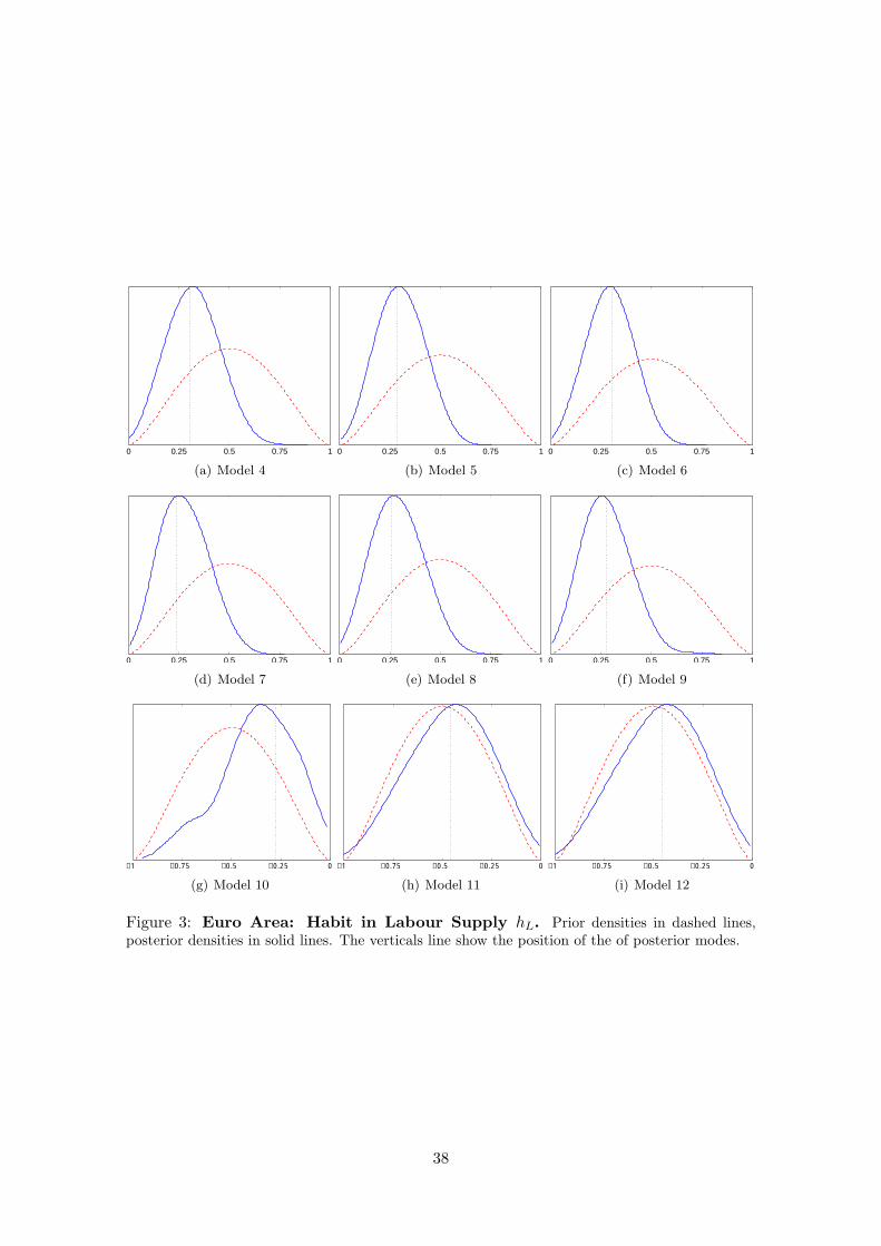
0 0.25 0.5 0.75 1

(a) Model 4

0 0.25 0.5 0.75 1

(b) Model 5

0 0.25 0.5 0.75 1

(c) Model 6

0 0.25 0.5 0.75 1

(d) Model 7

0 0.25 0.5 0.75 1

(e) Model 8

0 0.25 0.5 0.75 1

(f) Model 9

−1 −0.75 −0.5 −0.25 0

(g) Model 10

−1 −0.75 −0.5 −0.25 0

(h) Model 11

−1 −0.75 −0.5 −0.25 0

(i) Model 12

Figure 3: Euro Area: Habit in Labour Supply hL. Prior densities in dashed lines,posterior densities in solid lines. The verticals line show the position of the of posterior modes.

38

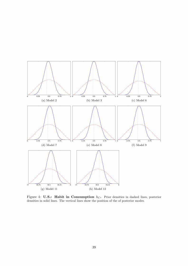
0 0.25 0.5 0.75 1

(a) Model 2

0 0.25 0.5 0.75 1

(b) Model 3

0 0.25 0.5 0.75 1

(c) Model 6

0 0.25 0.5 0.75 1

(d) Model 7

0 0.25 0.5 0.75 1

(e) Model 8

0 0.25 0.5 0.75 1

(f) Model 9

−1 −0.75 −0.5 −0.25 0

(g) Model 11

−1 −0.75 −0.5 −0.25 0

(h) Model 12

Figure 4: U.S.: Habit in Consumption hC . Prior densities in dashed lines, posteriordensities in solid lines. The vertical lines show the position of the of posterior modes.

39

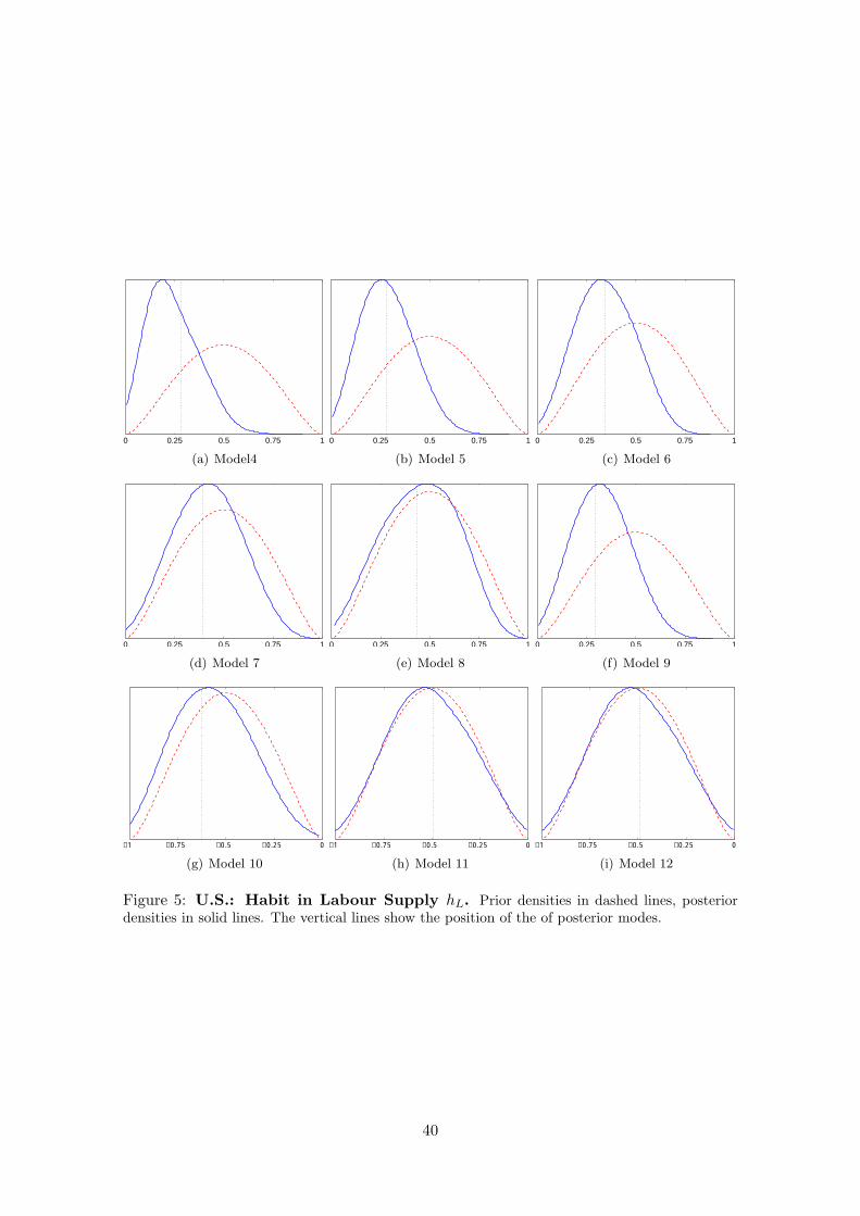
0 0.25 0.5 0.75 1

(a) Model4

0 0.25 0.5 0.75 1

(b) Model 5

0 0.25 0.5 0.75 1

(c) Model 6

0 0.25 0.5 0.75 1

(d) Model 7

0 0.25 0.5 0.75 1

(e) Model 8

0 0.25 0.5 0.75 1

(f) Model 9

−1 −0.75 −0.5 −0.25 0

(g) Model 10

−1 −0.75 −0.5 −0.25 0

(h) Model 11

−1 −0.75 −0.5 −0.25 0

(i) Model 12

Figure 5: U.S.: Habit in Labour Supply hL. Prior densities in dashed lines, posteriordensities in solid lines. The vertical lines show the position of the of posterior modes.

40