Relation Between Cash Rate

8/8/2019 Relation Between Cash Rate

http://slidepdf.com/reader/full/relation-between-cash-rate 1/37

THE LINK BETWEEN THE CASH RATE AND MARKET

INTEREST RATES

Philip Lowe

Research Discussion Paper

9504

May 1995

Economic Analysis Department

Reserve Bank of Australia

An earlier version of this paper was prepared for the autumn meeting of central bank

economists held by the Bank for International Settlements on 16-17 November

1993. I am indebted to Geoff Shuetrim and Nick de Roos for invaluable research

assistance and to colleagues at the Reserve Bank of Australia for comments and

discussion. The views are those of the author and are not necessarily those of the

Reserve Bank of Australia.



i

ABSTRACT

This paper explores the relationship between the cash rate and interest rates set by

financial intermediaries and interest rates set in auction markets. It presents

estimates of the average degree of pass-through of cash rate changes to these other

interest rates. It also presents a model of the spread between banks' lending rates

and the cash rate, and then uses the model to analyse developments in bank lending

spreads over recent years.

The paper argues that while banks' average lending spreads did not widen in the

early 1990s, the margin between lending rates and the cash rate did increase. It

examines the reasons for this change, paying particular attention to the roles played

by changes in the structure of banks' liabilities, changes in default probabilities and

changes in the degree of competition. The large lending spreads at the margin have

led to intensification of competition, particularly in the market for housing loans.

While these competitive pressures took some time to emerge, they are now playing

a role in the narrowing of margins.



ii

TABLE OF CONTENTS

1. Introduction 1

2. The Operation of Monetary Policy 3

3. The Pass-Through of Changes in the Cash Rate 4

3.1 Short-Term Money-Market Rates 9

3.2 Rates on Long-Term Securities 10

3.3 Deposit Rates 12

3.4 Lending Rates 13

4. What Determines the Degree of Pass-Through? 16

5. Conclusion 29

Appendix 1: Unit Root Tests 31

Appendix 2: Data 32

References 34



THE LINK BETWEEN THE CASH RATE AND MARKET

INTEREST RATES

Philip Lowe

1. INTRODUCTION

As an operating objective, Australian monetary policy is directed at affecting the

interest rate paid on overnight funds (the "cash rate"). The eventual impact that

changes in this interest rate have on the business cycle and inflation depends upon

how the changes are transmitted to other interest rates in the economy, and then

how those interest rates affect economic activity. This paper explores the first link in this chain - that is, the relationship between the cash rate and money-market

interest rates, bond rates and the interest rates paid and charged by financial

intermediaries.1 Given the importance of changes in lending rates in the monetary

transmission mechanism, the paper pays particular attention to the link between the

cash rate and banks' indicator lending rates.

In textbook discussions of the monetary transmission mechanism, the focus is

typically on the relationship between "the" interest rate and the real economy. Inreality, there is a whole range of interest rates that affects economic activity. While

the levels of the various interest rates tend to move together in the long run,

considerable divergence between movements often occurs in the short run. This is

seen most clearly in the shape of the yield curve, where sometimes, changes in

interest rates at the short end of the yield curve lead to long-term interest rates

moving in the opposite direction. Less dramatically, at the short end of the curve,

the interest rates paid and charged by intermediaries on variable-rate deposits/loans

seldom move immediately one for one with changes in the cash rate. The resulting

change in intermediaries' interest rate margins has been the subject of considerable

debate and comment over recent years.2

Many factors influence the reaction of market interest rates to changes in the cash

rate. For rates determined in auction markets, expectations of future changes in the

1 See Grenville (1993) for a recent summary of the details of the second link in the transmission

mechanism.

2 See for example Blundell-Wignall (1994), Harper (1994) and Moore (1994).



2

cash rate and expectations of future inflation are particularly important. For lending

and deposit rates set by intermediaries, the degree of competition is important, as

are the perceived riskiness of lending, the structure of intermediaries' liabilities and

the magnitude of operating costs and bank fees.

The spread between the average interest rate charged by banks and their average

cost of funds has shown little change over the past decade. By international

standards, this spread is relatively high, although this largely compensates for the

fact that fee and non-interest income is relatively low.3 While the comparison of

average deposit and lending rates is important for assessing bank profitability,

examining changes in spreads between lending rates and the marginal cost of funds

(approximated by the cash rate) can help in understanding the dynamics of bank

competition.

The spreads between lending rates and the cash rate tend to fluctuate more than

average spreads. In the late 1980s, the spread between the banks' typical indicator

rate for business lending and the cash rate, averaged around 2 per cent. This spread

widened to over 4 per cent in late 1991, only narrowing significantly in late 1994.

Large movements have also occurred in the spread between the standard interest

rate on variable-rate mortgages and the cash rate. These changes in marginal

lending spreads have had little impact on the average spread, as the margin betweenthe cash rate and deposit rates narrowed around the same time that the marginal

lending spreads widened.

The relatively large marginal lending spreads in the early 1990s meant that lending

for housing, in particular, was very profitable. Initially this was not reflected in

widespread profitability of the banking sector, as many banks were suffering the

consequences of the bad loans made in the late 1980s, and the adverse effects of a

change in the structure of their deposits. As the bad debts problem receded, the

profitability of lending became increasingly apparent. A number of new competitors

entered the market and existing institutions shaved their margins, particularly for

new customers.

The intensification in the degree of competition, especially from new entrants, has

been particularly evident in the market for housing finance. This competition, while

3 For a more detailed discussion of average interest rate margins see Reserve Bank of Australia

(1994).



3

taking time to develop, has played some role in the recent narrowing of margins.

The entry of new providers of finance for small business has been much slower,

despite the existence of relatively large margins. To a considerable extent this

reflects the difficulty in developing the capability to undertake the necessary

information assessment needed for successful lending to small business. In contrast,

lending for housing requires the collection and evaluation of relatively few pieces of

information, and the resulting lower information costs have allowed finance

providers to enter the housing-finance market in response to profitable opportunities

at the margin.

The remainder of this paper analyses the relationship between the cash rate and

market interest rates. Section 2 briefly describes the role that the cash rate plays in

the operating procedures for Australian monetary policy. Section 3 examines theextent to which, on average, changes in the cash rate are "passed through" to other

interest rates in the economy. Section 4 presents a model of the relationship

between the cash rate and bank lending rates and then analyses the factors that have

led to recent changes in the spreads between key indicator lending rates and the

cash rate. Finally, Section 5 presents a summary and conclusions.

2. THE OPERATION OF MONETARY POLICY

Monetary policy operates via the Bank influencing the interest rate paid on

overnight funds (the "cash rate").4 Changes in this rate affect the entire structure of

interest rates in the economy. The Bank's influence over the cash rate comes from

its ability to control the availability of funds used to settle transactions between

financial institutions. By undertaking open market operations, principally in

government securities with less than one year to maturity, the Bank controls the

availability of settlement funds and hence the interest rate paid on overnight

deposits.5

Prior to January 1990, the Bank did not announce its desired level for the cash rate.

Instead it signalled the desired level by operating in the market for settlement funds,

which meant that there was considerable daily volatility in the cash rate. This

4 See Rankin (1992) for a detailed description of the structure of the market for overnight funds.

5 Securities are traded outright and through repurchase agreements. On occasions, the Bank also utilises the foreign currency swap market.



4

operating system had the advantage of allowing policy to be changed in a relatively

low-key manner, but it had the disadvantage of sometimes making it difficult for the

market and others to distinguish between noise and a change in policy.

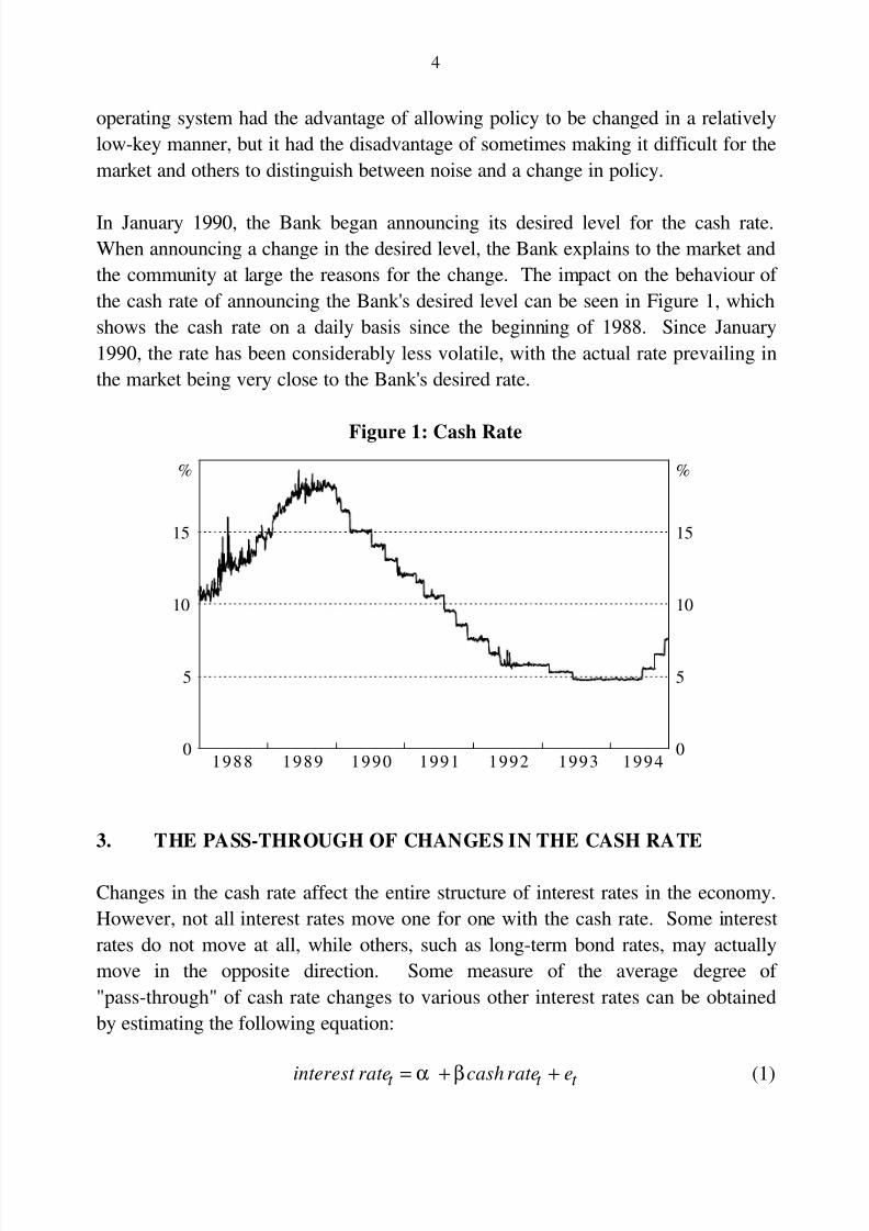
In January 1990, the Bank began announcing its desired level for the cash rate.

When announcing a change in the desired level, the Bank explains to the market and

the community at large the reasons for the change. The impact on the behaviour of

the cash rate of announcing the Bank's desired level can be seen in Figure 1, which

shows the cash rate on a daily basis since the beginning of 1988. Since January

1990, the rate has been considerably less volatile, with the actual rate prevailing in

the market being very close to the Bank's desired rate.

Figure 1: Cash Rate

0

5

10

15

0

5

10

15

% %

1994199319921991199019891988

3. THE PASS-THROUGH OF CHANGES IN THE CASH RATE

Changes in the cash rate affect the entire structure of interest rates in the economy.

However, not all interest rates move one for one with the cash rate. Some interest

rates do not move at all, while others, such as long-term bond rates, may actually

move in the opposite direction. Some measure of the average degree of

"pass-through" of cash rate changes to various other interest rates can be obtained

by estimating the following equation:

interest rate cash rate et t t = + +α β (1)



5

If pass-through is instantaneous and complete, β should be insignificantly different

from one. In practice, the pass-through of cash rate changes may not be

instantaneous. In particular, rates widely advertised by the banks may take longer

to adjust than rates determined in continuously operating auction markets. To allow

for this possibility, we also estimate the following model:

interest rate cash rate interest rate cash ratet ii

t i ii

t i t t = + ∑ + ∑ + +=

−=

−α γ ϕ δ ε0

3

0

3∆ ∆ (2)

The long-run response of the relevant interest rate to a change in the cash rate is

given by the parameter δ.



6

Table 1: Interest Rate Pass-Through

Levels1 Differences1Long-Run

α β R2 α β R

2Pass-Through2

(δ )

Money-market rates

3-6-month CD 0.32(0.14)

0.97(0.02)

0.98 -0.03(0.03)

0.70(0.07)

0.54 0.97(0.03)

90-day bank bill 0.09(0.15)

0.99(0.01)

0.99 -0.01(0.02)

0.88(0.06)

0.68 0.91(0.09)

180-day bank bill 0.39(0.25)

0.96(0.02)

0.98 -0.02(0.04)

0.67(0.10)

0.40 0.87(0.16)

13-week treasury note 0.24(0.18)

0.94(0.02)

0.98 -0.03(0.05)

0.68(0.11)

0.32 0.94(0.02)

Long-term bonds

2-year treasury bonds 2.89(0.44)

0.70(0.03)

0.93 -0.02(0.05)

0.27(0.08)

0.07 0.70(0.08)


0.56(0.04)

0.90 -0.02(0.05)

0.18(0.09)

0.03 0.55(0.09)


0.46(0.04)

0.85 -0.02(0.04)

0.11(0.09)

0.01 0.46(0.07)

Deposit rates

Cash management trust -0.72(0.20)

0.96(0.02)

0.98 -0.06(0.05)

0.31(0.09)

0.20 1.06(0.09)

Low-balance accounts -0.82(0.20)

0.55(0.02)

0.98 -0.05(0.03)

0.27(0.08)

0.19 0.56(0.03)

High-balance accounts -0.25(0.25)

0.77(0.02)

0.95 -0.06(0.03)

0.22(0.09)

0.18 0.85(0.12)

1-month fixed deposit 1.08(0.26)

0.75(0.03)

0.94 -0.05(0.05)

0.22(0.10)

0.05 0.78(0.02)

1-year fixed deposit 1.54(0.30)

0.78(0.03)

0.96 -0.02(0.04)

0.34(0.10)

0.25 0.75(0.10)

Lending rates

Business indicator rate 5.07(0.12)

0.83(0.01)

0.99 -0.03(0.03)

0.58(0.07)

0.62 0.89(0.08)

Housing rate 6.89(0.38)

0.56(0.04)

0.88 -0.02(0.04)

0.11(0.05)

0.02 0.65(0.03)

Personal instalment rate 13.10(0.47)

0.52(0.04)

0.88 -0.03(0.04)

0.09(0.04)

0.02 0.68(0.06)

Credit card rate 17.33(1.40)

0.36(0.10)

0.35 -0.06(0.05)

0.01(0.05)

-0.01 1.85(1.09)

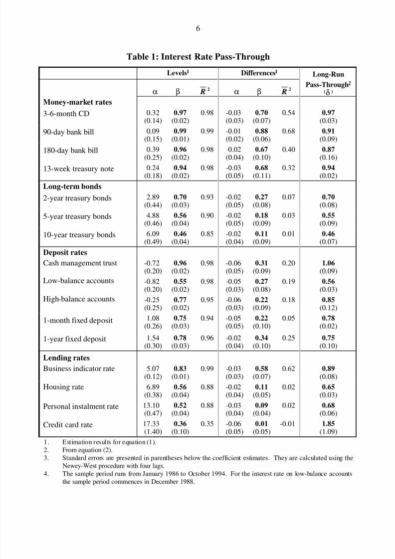
1. Estimation results for equation (1).2. From equation (2).3. Standard errors are presented in parentheses below the coefficient estimates. They are calculated using the

Newey-West procedure with four lags.4. The sample period runs from January 1986 to October 1994. For the interest rate on low-balance accounts

the sample period commences in December 1988.



7

Equation (1) is estimated by ordinary least squares and equation (2) by instrumental

variables using monthly data over the period from January 1986 to October 1994.6

The sample period is constrained by the fact that prior to April 1985 most lending

rates were the subject of regulation.7 We chose January 1986 as the starting point

to allow for a period of adjustment to the deregulated environment. Equation (1) is

estimated in both levels and differences. The results are reported in Table 1. For

the autoregressive distributed lag model we simply report the estimate of the

long-run response.8

In discussing the extent of "pass-through" it is useful to distinguish among four

classes of interest rates:

• short-term money-market rates;

• rates on long-term securities;

• deposit rates;

• lending rates.

We discuss each of these in turn. Figure 2 shows the various interest rates.

6 In estimating (2), the lagged interest rate is used as the instrument for the current change in the

interest rate.

7 While the regulation of most lending rates was lifted in April 1985, the ceiling on new owner-occupied housing loans was not removed until April 1986. The interest rate on overdraftsgreater than $50,000 was lifted in February 1972. In February 1976, the threshold level was

increased to $100,000. Interest rate ceilings on all trading and savings bank deposits wereremoved in December 1980.

8 We take an agnostic view with respect to the order of integration of the various interest rates.Appendix 1 reports the results of unit root tests using the Augmented Dickey-Fuller test. Forall interest rates it is not possible to reject the unit root null hypothesis. The Appendix also

reports the results of co-integration tests (using the Unrestricted Error-Correction Model)between the cash rate and various interest rates. For some interest rates it is possible to rejectthe null hypothesis that the rate is co-integrated with the cash rate while for others it is not

possible to do so. Given the relatively low power of the tests, especially when the sampleperiod is relatively short, the results should be interpreted with caution. If interest rates areindeed non-stationary, it would be surprising if some rates were co-integrated with the cash

rate, while others were not. It would also be surprising if the true long-run response wassubstantially different from one.



8

Figure 2: Interest Rates

4

8

12

16

20

24

Cash rate

3-6 month CDs

180-day bank bills

13-week treasury notes

Money-market rates% %

0

4

8

12

16

20

24Cash rate

Low-balance a/c

High-balance a/c

Cash mgt trusts

1-month fixed dep

1-year fixed dep

0

4

8

12

16

20

24

Cash rate

Business indicator rate

Housing rate

Personal instalment rate

Credit card rate

Lending ratesDeposit rates%%

4

8

12

16

20

24

Cash rate

2-yr treasury bonds

5-yr treasury bonds

10-yr treasury bonds

Long-term bonds

19911988 199419911988 1994



9

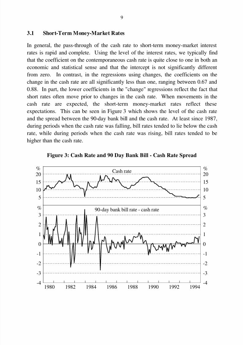
3.1 Short-Term Money-Market Rates

In general, the pass-through of the cash rate to short-term money-market interest

rates is rapid and complete. Using the level of the interest rates, we typically find

that the coefficient on the contemporaneous cash rate is quite close to one in both aneconomic and statistical sense and that the intercept is not significantly different

from zero. In contrast, in the regressions using changes, the coefficients on the

change in the cash rate are all significantly less than one, ranging between 0.67 and

0.88. In part, the lower coefficients in the "change" regressions reflect the fact that

short rates often move prior to changes in the cash rate. When movements in the

cash rate are expected, the short-term money-market rates reflect these

expectations. This can be seen in Figure 3 which shows the level of the cash rate

and the spread between the 90-day bank bill and the cash rate. At least since 1987,during periods when the cash rate was falling, bill rates tended to lie below the cash

rate, while during periods when the cash rate was rising, bill rates tended to be

higher than the cash rate.

Figure 3: Cash Rate and 90 Day Bank Bill - Cash Rate Spread

5

10

15

20

5

1015

20

-4

-3

-2

-1

0

1

2

3

-4

-3

-2

-1

0

1

2

3

Cash rate

90-day bank bill rate - cash rate

19941992199019881986198419821980

% %

% %



10

3.2 Rates on Long-Term Securities

The relationship between the cash rate and the longer end of the yield curve is more

complex. Changes in the cash rate affect the expected future level of short rates,

and thus the current level of long rates, in two ways. The first channel is oftenreferred to as the liquidity effect - lower short rates today imply lower short rates for

some period into the future. As a result, the lower short rates today put downward

pressure on long-term bond rates. The second channel works primarily through

changing expectations of future inflation. If a lowering of the cash rate generates

expectations of higher future inflation, short-term rates will be expected to increase

at some point in the future. This will put upward pressure on nominal long-term

bond rates that may offset the impact of lower short rates in the near term.

The second block of Table 1 reports the interest rate pass-through regressions for

two, five and ten-year government bonds. The long-run pass-through coefficient

and the coefficient on the cash rate in the "levels" regressions are positive for all

three rates, but the size of the coefficients declines the longer is the maturity of the

security. On average, over the sample period, higher cash rates have tended to be

associated with higher rates on government bonds. Given that the liquidity effect is

relatively more important the shorter is the maturity, it is not surprising that the rates

on shorter maturities are more responsive to changes in the cash rate than is the

10-year rate.

The results using the changes in interest rates are less clear cut, particularly for the

ten-year bond. The two-year bond is the only one to have a significant positive

coefficient on changes in the current cash rate. The contrasting results from the

levels and difference equations suggest that while long-term bonds eventually move

in the same direction as the cash rate, the timing of movements in the cash rate and

bond rates often differs. Indeed, the relationship between bond rates and the cash

rate changes through time. During some periods, bond rates tend to move in thesame direction as the cash rate, while during others, they move in the opposite

direction.

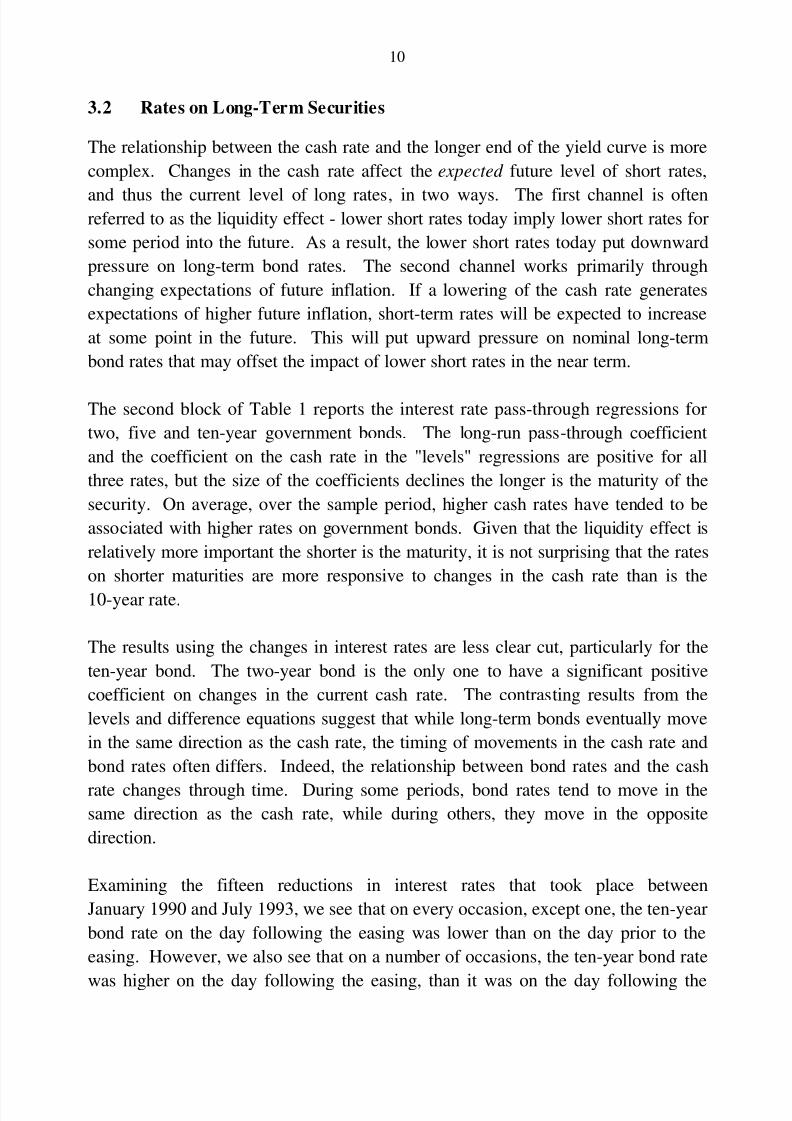
Examining the fifteen reductions in interest rates that took place between

January 1990 and July 1993, we see that on every occasion, except one, the ten-year

bond rate on the day following the easing was lower than on the day prior to the

easing. However, we also see that on a number of occasions, the ten-year bond rate

was higher on the day following the easing, than it was on the day following the



11

previous easing (see Figure 4). In particular, the reductions in the first three

quarters of 1990 saw some net increase in long-term bond rates. In contrast, from

the last quarter of 1990, bond rates tended to move in the same downward direction

as the cash rate. To a large extent, this change in behaviour can be attributed to a

progressive reduction in inflation expectations. The easings in the first three

quarters of 1990 were made prior to progress on inflation being widely apparent.

However, from late 1990 onwards, it became clearer that the economy was weaker

than had been expected and that there had been a structural break in inflation.

Accordingly, reductions in the cash rate did not lead to expectations of higher future

inflation, and bond rates fell.

More recently, long-term bond rates increased by about 3 percentage points over the

first half of 1994, despite no change in the cash rate. This increase reflected higherexpected future short rates, as expectations of future real rates and future inflation

were revised upwards. When the cash rate was increased by 2.75 percentage points

between August and December 1994, long bond rates rose by a further 1 percentage

point. At the end of 1994, however, long bond rates were below their levels in early

October 1994, even though cash rates had risen by 2 percentage points over that

period. Clearly, while cash rates and bond rates tend to move together over the

longer term, expectations about future inflation can lead to very weak short-run

linkages between changes in the cash rate and bond yields.

An additional factor influencing the relationship between the short and long ends of

the yield curve is the behaviour of world real long-term interest rates. Australia

cannot isolate itself from the effects of a change in world real long interest rates,

particularly due to changes in world inflation and savings-investment patterns.

Higher world real long interest rates mean higher Australian real long rates. While

such a change might be expected to eventually flow through to short rates (reversing

the direction of "causation" discussed above), this process may be drawn out over a

considerable period of time.



12

Figure 4: Yield Curve (Day After Policy Change)

Overnight 6 months 3 years 10 years4

6

8

10

12

14

16

Overnight 6 months 3 years 10 years4

6

8

10

12

14

16

24 January 1990

5 April 1990

16 February 1990

3 August 1990

16 October 1990

5 April 1991

19 December 1990

17 May 1991

4 September 1991

7 May 1992

9 January 1992

7 November 1991

9 July 1992

24 March 1993

2 August 1993

18 August 1994

25 October 1994

15 December 1994

% %

3.3 Deposit Rates

We now turn to an examination of the relationship between the cash rate and deposit

rates. We examine three different classes of deposits: cash management trusts,transaction - investment accounts and fixed deposits. The estimation results are

presented in the third block of Table 1. The cash management trusts have the most

responsive interest rates. This is hardly surprising as they invest almost entirely in

short-term money-market instruments. The interest rates on these accounts behave

similarly to the money-market rates, with the exception that, on average, the rates

paid by cash management trusts tend to be slightly lower than the cash rate (the

intercept is significantly less than zero). This reflects the management expenses of

the trust.



13

The picture is somewhat different for the interest rates paid on the transaction -

investment accounts. These rates adjust much less to changes in the cash rate than

do the money-market interest rates. The interest rates paid on the low-balance

accounts are particularly sticky. Competition for these accounts is relatively

limited. They tend to have high operating costs and the accounts are held by

depositors with relatively low interest-rate sensitivity. Competition for accounts

with larger balances is more aggressive, and hence deposit rates on these accounts

tend to move more closely in line with the rates on alternative investments such as

cash management trusts. Nevertheless, the adjustment in rates appears to be slower

than that for money-market rates. The pass-through of cash rate changes to

one-month and one-year fixed deposits is similar to that for the high-balance

transaction accounts, although the long-run pass-through appears smaller. The

estimates of α also indicate that, on average, these fixed deposits pay a higher rateof interest than that paid on transaction accounts.

3.4 Lending Rates

Finally, we turn to the lending rates. Changes in the cash rate are not always passed

through completely and immediately into lending rates. This can be seen in the final

section of Table 1. It shows quite different degrees of pass-through for the four loan

rates examined. The stickiest interest rate is the rate on credit cards. Between

January 1986 and October 1994, the credit card rate ranged between 14.4 per centand 24.7 per cent whereas the cash rate varied in a range between 4.75 per cent and

18.9 per cent. The rates on personal instalment finance and housing loans also tend

not to move one for one with the cash rate. This is the case in both the short run

and the long run. Finally, while the business indicator rate is the least sticky loan

rate, changes in the cash rate do not appear to be always completely passed through.

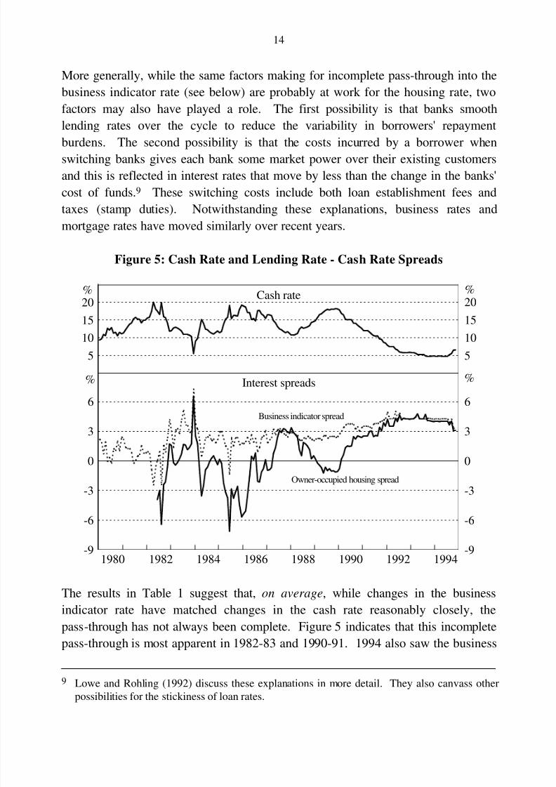
Figure 5 shows the spreads between the business indicator rate and the cash rate

and between the owner-occupied housing rate and the cash rate. It also shows the

level of the cash rate. Given the lower pass-through of changes in the cash rate to

the housing rate, it is hardly surprising that the housing - cash rate spread has been

more volatile than the business indicator - cash rate spread. When cash rates

reached their 1982, 1985 and 1989 peaks, the housing rate actually lay below the

cash rate. In the earlier episodes, the large negative spread was in part a direct

result of the regulation of housing interest rates and in 1989, the fact that mortgage

rates did not move up one for one with the cash rate, partly reflected changes in the

arrangements for banks' Non-callable Deposits with the Reserve Bank.



14

More generally, while the same factors making for incomplete pass-through into the

business indicator rate (see below) are probably at work for the housing rate, two

factors may also have played a role. The first possibility is that banks smooth

lending rates over the cycle to reduce the variability in borrowers' repayment

burdens. The second possibility is that the costs incurred by a borrower when

switching banks gives each bank some market power over their existing customers

and this is reflected in interest rates that move by less than the change in the banks'

cost of funds.9 These switching costs include both loan establishment fees and

taxes (stamp duties). Notwithstanding these explanations, business rates and

mortgage rates have moved similarly over recent years.

Figure 5: Cash Rate and Lending Rate - Cash Rate Spreads

5

10

15

20

5

10

15

20

-9

-6

-3

0

3

6

-9

-6

-3

0

3

6

Cash rate

Interest spreads

Business indicator spread

Owner-occupied housing spread

19941992199019881986198419821980

% %

% %

The results in Table 1 suggest that, on average, while changes in the business

indicator rate have matched changes in the cash rate reasonably closely, the

pass-through has not always been complete. Figure 5 indicates that this incomplete

pass-through is most apparent in 1982-83 and 1990-91. 1994 also saw the business

9 Lowe and Rohling (1992) discuss these explanations in more detail. They also canvass other

possibilities for the stickiness of loan rates.



15

indicator rate move by less than the cash rate, unwinding much of the increase in the

spread in 1990-91. Outside these periods, changes in the indicator rate appear to

have matched changes in the cash rate quite closely. Overall, relative to the size of

the changes in the cash rate, changes in the margin have been relatively small.

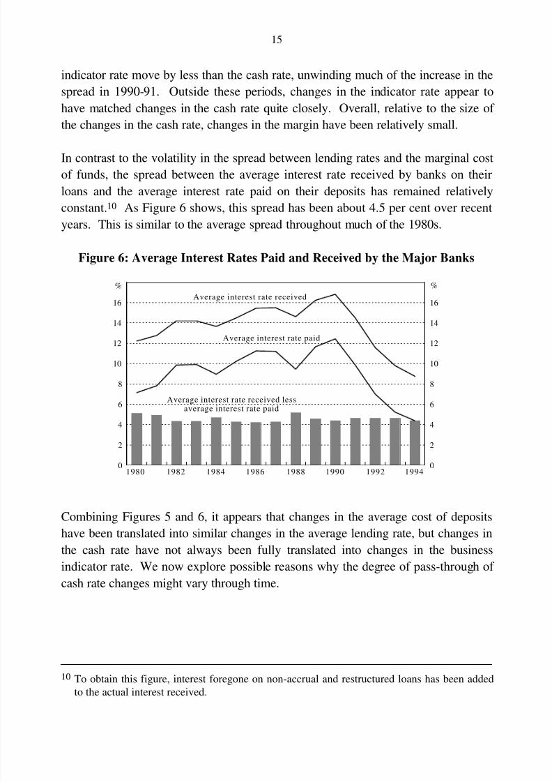
In contrast to the volatility in the spread between lending rates and the marginal cost

of funds, the spread between the average interest rate received by banks on their

loans and the average interest rate paid on their deposits has remained relatively

constant.10 As Figure 6 shows, this spread has been about 4.5 per cent over recent

years. This is similar to the average spread throughout much of the 1980s.

Figure 6: Average Interest Rates Paid and Received by the Major Banks

0

2

4

6

8

10

12

14

16

0

2

4

6

8

10

12

14

16Average interest rate received

Average interest rate paid

Average interest rate received less

average interest rate paid

19941992199019881986198419821980

% %

Combining Figures 5 and 6, it appears that changes in the average cost of deposits

have been translated into similar changes in the average lending rate, but changes in

the cash rate have not always been fully translated into changes in the businessindicator rate. We now explore possible reasons why the degree of pass-through of

cash rate changes might vary through time.

10 To obtain this figure, interest foregone on non-accrual and restructured loans has been added

to the actual interest received.



16

4. WHAT DETERMINES THE DEGREE OF PASS-THROUGH?

What factors determine the degree to which a change in the cash rate is passed

through to banks' indicator lending rates? Below we focus on the following three

(not mutually exclusive) explanations:

(i) the structure of banks' deposits and interest rates;

(ii) the riskiness of bank lending;

(iii) the degree of competition in banking.

We use the following simple framework to examine how these factors might affect

the relationship between indicator lending rates and the cash rate. By assuming thatthe loan rate is set to equalise the expected return from the loan with the cost of the

providing the loan (including the return on capital) we have:

r p q r r cl c d + = + + − + +α α( ) ( )( )1 1 1 (3)

where: r l = loan rate;

p = probability that interest is paid;

q = probability that the loan principal is repaid;

α = capital requirement;

r c = rate of return to capital;

r d = interest rate paid on deposits;

c = administrative costs of providing a loan (less fee income).

The expected gross return from lending one dollar (the left hand side of (3)) consists

of two components: the expected interest payments (r l p) and the expected principal

repayment (q). If there is no default risk ( p = q = 1), the gross return from lending

one dollar will be r l+1.

The "cost" of providing the loan is given by the right hand side of (3). Each dollar

of loans is funded using a fraction α of capital and 1-α of deposits. Thus, the cost

of providing the loan consists of three components: the amount that must be paid to



17

the owners of the capital ( ( ))α 1+ r c

, the amount that must be paid to depositors

(( )( ))1 1− +α r d

and operating or administrative costs (c).

Re-arranging (3), we obtain an expression for the lending rate:

r r r c q

plc d =

+ − + + −

α α( ) ( )1 1(4)

So far we have treated all deposits as attracting the same interest rate (r d ). As

discussed above, the costs of various types of deposits do not always move

together, with short-term money-market interest rates moving much more closely

with the cash rate than do rates on many other classes of deposits. For the sake of

simplicity, we assume that there are two types of deposits; deposits that attract an

interest rate equal to the cash rate and deposits that attract lower and less variable

interest rates than the cash rate. Thus, the average cost of deposits is given by:

r r r d cash low= + −β β( )1 (5)

where: r cash = cash rate;

r low = average interest rate on the low-interest rate deposits.

Substituting (5) into (4) and rearranging we can obtain an expression for the

difference between the lending rate and the cash rate. This is given by the

following:

r r p

r r c q r r p r l cash c d cash low cash− = − + + − − − − + −1

1 1 1α β( ) ( ) ( )( ) ( ) (6)

From this equation it can be seen that the spread between the lending rate and thecash rate will increase if:

(i) the required return to capital increases relative to the average rate on bank

deposits (i.e., r c-r d increases);

(ii) the share of loans funded by capital increases (i.e., α increases);

(iii) administrative costs increase (i.e., c increases);



18

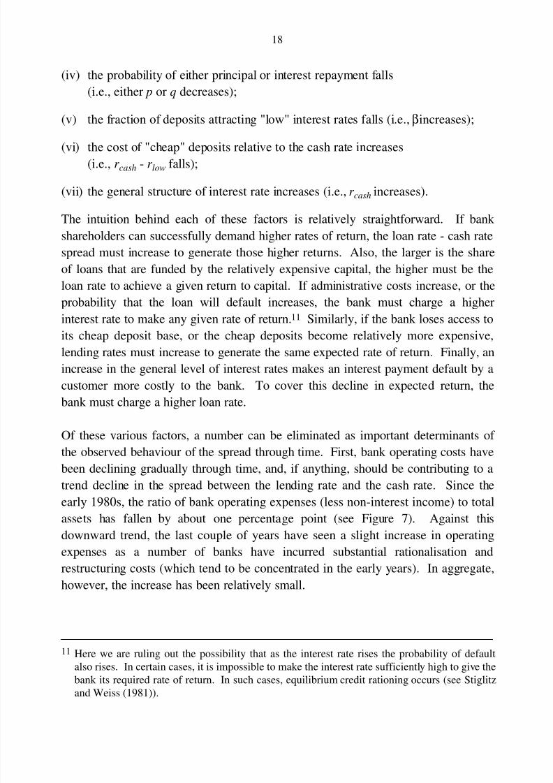
(iv) the probability of either principal or interest repayment falls

(i.e., either p or q decreases);

(v) the fraction of deposits attracting "low" interest rates falls (i.e., βincreases);

(vi) the cost of "cheap" deposits relative to the cash rate increases

(i.e., r cash - r low falls);

(vii) the general structure of interest rate increases (i.e., r cash increases).

The intuition behind each of these factors is relatively straightforward. If bank

shareholders can successfully demand higher rates of return, the loan rate - cash rate

spread must increase to generate those higher returns. Also, the larger is the share

of loans that are funded by the relatively expensive capital, the higher must be theloan rate to achieve a given return to capital. If administrative costs increase, or the

probability that the loan will default increases, the bank must charge a higher

interest rate to make any given rate of return.11 Similarly, if the bank loses access to

its cheap deposit base, or the cheap deposits become relatively more expensive,

lending rates must increase to generate the same expected rate of return. Finally, an

increase in the general level of interest rates makes an interest payment default by a

customer more costly to the bank. To cover this decline in expected return, the

bank must charge a higher loan rate.

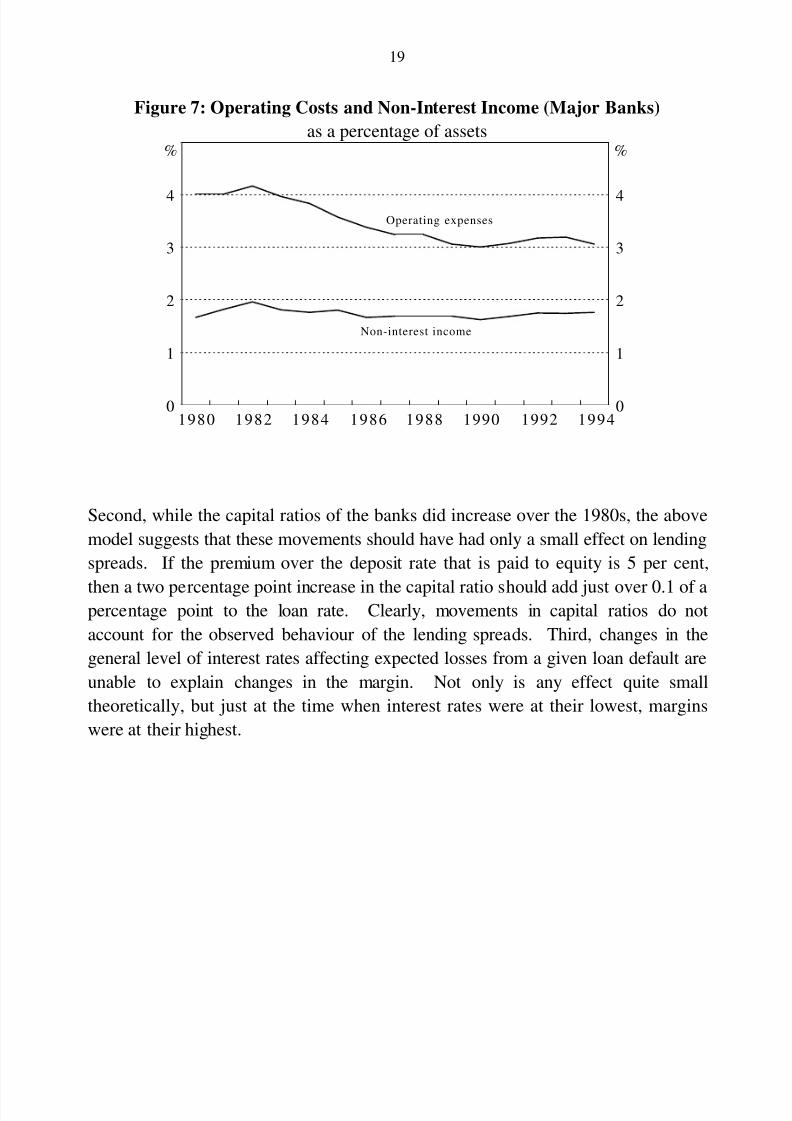
Of these various factors, a number can be eliminated as important determinants of

the observed behaviour of the spread through time. First, bank operating costs have

been declining gradually through time, and, if anything, should be contributing to a

trend decline in the spread between the lending rate and the cash rate. Since the

early 1980s, the ratio of bank operating expenses (less non-interest income) to total

assets has fallen by about one percentage point (see Figure 7). Against this

downward trend, the last couple of years have seen a slight increase in operating

expenses as a number of banks have incurred substantial rationalisation andrestructuring costs (which tend to be concentrated in the early years). In aggregate,

however, the increase has been relatively small.

11 Here we are ruling out the possibility that as the interest rate rises the probability of default

also rises. In certain cases, it is impossible to make the interest rate sufficiently high to give the

bank its required rate of return. In such cases, equilibrium credit rationing occurs (see Stiglitzand Weiss (1981)).



19

Figure 7: Operating Costs and Non-Interest Income (Major Banks)

as a percentage of assets

0

1

2

3

4

0

1

2

3

4

% %

19941992199019881986198419821980

Operating expenses

Non-interest income

Second, while the capital ratios of the banks did increase over the 1980s, the above

model suggests that these movements should have had only a small effect on lending

spreads. If the premium over the deposit rate that is paid to equity is 5 per cent,

then a two percentage point increase in the capital ratio should add just over 0.1 of apercentage point to the loan rate. Clearly, movements in capital ratios do not

account for the observed behaviour of the lending spreads. Third, changes in the

general level of interest rates affecting expected losses from a given loan default are

unable to explain changes in the margin. Not only is any effect quite small

theoretically, but just at the time when interest rates were at their lowest, margins

were at their highest.



20

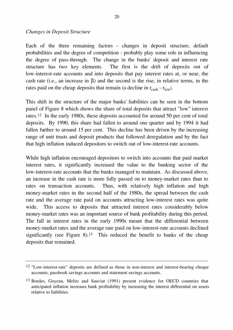
Changes in Deposit Structure

Each of the three remaining factors - changes in deposit structure, default

probabilities and the degree of competition - probably play some role in influencing

the degree of pass-through. The change in the banks' deposit and interest rate

structure has two key elements. The first is the drift of deposits out of

low-interest-rate accounts and into deposits that pay interest rates at, or near, the

cash rate (i.e., an increase in β) and the second is the rise, in relative terms, in the

rates paid on the cheap deposits that remain (a decline in rcash - rlow).

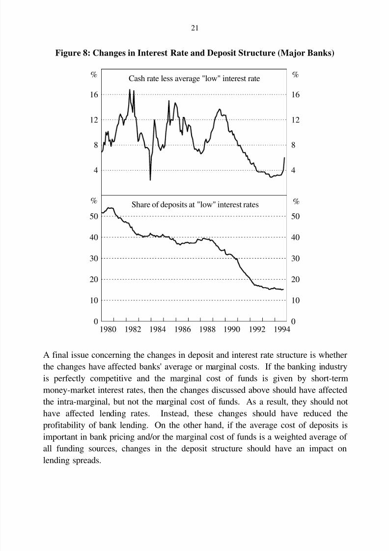
This shift in the structure of the major banks' liabilities can be seen in the bottom

panel of Figure 8 which shows the share of total deposits that attract "low" interest

rates.12 In the early 1980s, these deposits accounted for around 50 per cent of totaldeposits. By 1990, this share had fallen to around one quarter and by 1994 it had

fallen further to around 15 per cent. This decline has been driven by the increasing

range of unit trusts and deposit products that followed deregulation and by the fact

that high inflation induced depositors to switch out of low-interest-rate accounts.

While high inflation encouraged depositors to switch into accounts that paid market

interest rates, it significantly increased the value to the banking sector of the

low-interest-rate accounts that the banks managed to maintain. As discussed above,an increase in the cash rate is more fully passed on to money-market rates than to

rates on transaction accounts. Thus, with relatively high inflation and high

money-market rates in the second half of the 1980s, the spread between the cash

rate and the average rate paid on accounts attracting low-interest rates was quite

wide. This access to deposits that attracted interest rates considerably below

money-market rates was an important source of bank profitability during this period.

The fall in interest rates in the early 1990s meant that the differential between

money-market rates and the average rate paid on low-interest-rate accounts declined

significantly (see Figure 8).13 This reduced the benefit to banks of the cheap

deposits that remained.

12 "Low-interest-rate" deposits are defined as those in non-interest and interest-bearing cheque

accounts, passbook savings accounts and statement savings accounts.

13 Bordes, Goyeau, Melitz and Sauviat (1991) present evidence for OECD countries that

anticipated inflation increases bank profitability by increasing the interest differential on assetsrelative to liabilities.



21

Figure 8: Changes in Interest Rate and Deposit Structure (Major Banks)

4

8

12

16

4

8

12

16

0

10

20

30

40

50

0

10

20

30

40

50

% %

% %

Cash rate less average "low" interest rate

Share of deposits at "low" interest rates

19941992199019881986198419821980

A final issue concerning the changes in deposit and interest rate structure is whether

the changes have affected banks' average or marginal costs. If the banking industry

is perfectly competitive and the marginal cost of funds is given by short-term

money-market interest rates, then the changes discussed above should have affected

the intra-marginal, but not the marginal cost of funds. As a result, they should not

have affected lending rates. Instead, these changes should have reduced the

profitability of bank lending. On the other hand, if the average cost of deposits is

important in bank pricing and/or the marginal cost of funds is a weighted average of

all funding sources, changes in the deposit structure should have an impact on

lending spreads.



22

Certainly Figure 6 suggests that the average cost of bank deposits has been an

important factor in the pricing of bank loans. The reduction in the cash rate between

1990 and 1993 was larger than the reduction in the average cost of deposits due to

the stickiness of many deposit rates. Because average deposit rates adjust less than

the cash rate, loan rates also adjust less than the cash rate. As a result, the spread

between the cash rate and the loan rate widened as the cash rate fell. This

explanation leaves unresolved the important question of bank competition. To some

extent, the combination of lower inflation and increased competition for deposits

should have led to a reduction in the difference between the average interest rate

received and paid, and in so doing, reduced the profitability of core lending

business. Working in the other direction, strong demand for housing loans may

have meant that banks could maintain these margins. These issues are discussed in

more detail below.

The Riskiness of Lending

The second factor that probably plays some role in influencing the degree of

pass-through is the perceived riskiness of bank lending. In Figure 5, the lending

spread appears to behave counter-cyclically - in particular, the periods of slow

economic activity are associated with the largest lending spreads. If periods of

recessed activity are associated with a higher probability of loan default (that is, alower p or q) then it is natural for lending spreads to widen in recessions.

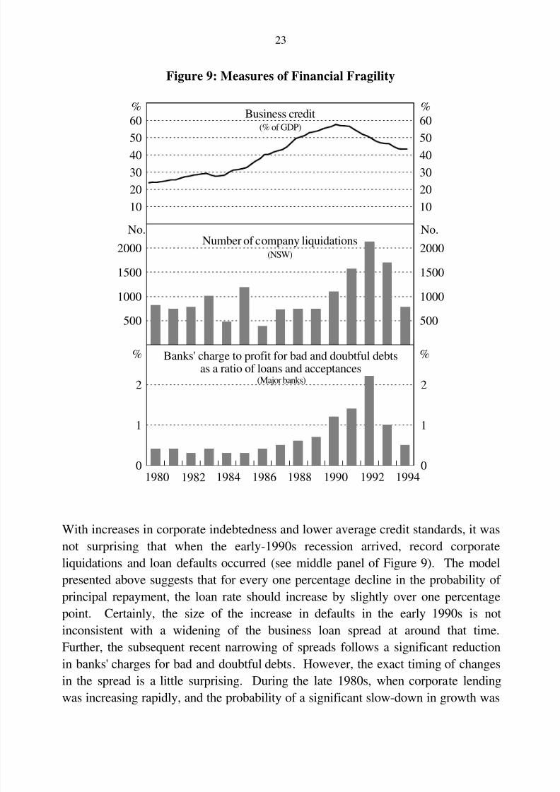
Prior to deregulation of the financial markets, banks had to ration credit. Those

customers with the highest credit rating stood at the front of the queue. As a result,

loan defaults were relatively rare (see bottom panel of Figure 9). Following

deregulation, the need for regulation-induced credit rationing no longer existed and

banks engaged in aggressive competition for business. On the demand side,

increasing asset prices and the weakening of financial constraints saw significant

increases in demand for intermediated finance from the corporate sector. These

increased demands were willingly met by the newly deregulated banking sector.

The result of this process was a significant increase in the gearing of the corporate

sector and an increase in the ratio of business credit outstanding to GDP (see top

panel of Figure 9).



23

Figure 9: Measures of Financial Fragility

10

20

30

4050

60

10

20

30

4050

60

500

10001500

2000

500

10001500

2000

0

1

2

0

1

2

% %

% %

Business credit(% of GDP)

Number of company liquidations(NSW)

Banks' charge to profit for bad and doubtful debtsas a ratio of loans and acceptances

(Major banks)

No.No.

1994199219901988198619841980 1982

With increases in corporate indebtedness and lower average credit standards, it was

not surprising that when the early-1990s recession arrived, record corporate

liquidations and loan defaults occurred (see middle panel of Figure 9). The model

presented above suggests that for every one percentage decline in the probability of

principal repayment, the loan rate should increase by slightly over one percentage

point. Certainly, the size of the increase in defaults in the early 1990s is not

inconsistent with a widening of the business loan spread at around that time.

Further, the subsequent recent narrowing of spreads follows a significant reduction

in banks' charges for bad and doubtful debts. However, the exact timing of changes

in the spread is a little surprising. During the late 1980s, when corporate lending

was increasing rapidly, and the probability of a significant slow-down in growth was



24

rising, there was no widening of the spread. Certainly with hindsight it appears that

during the final stages of the boom, lending was becoming more and more risky as

the likelihood of a fall in asset prices and a recession increased. However, it was

only after the recession hit, and the banks experienced record bad debts, that

spreads widened. Similarly, margins have narrowed only after bad debts expenses

have declined. This suggests that the banks may have been under-pricing risk

during the late 1980s and over-pricing risk in the first half of the 1990s.14

If changes in the riskiness of bank lending are responsible for change in margins, it

suggests that banks have not been undertaking "dynamic provisioning"; that is, at

the top of a boom, they have not increased loan margins and provisions in

expectation of higher future loan defaults and they have not reduced margins and

provisions at the bottom of the cycle. Instead it appears that pricing andprovisioning is static, with margins only being changed once a change in default

experience actually occurs.

Competition

A third possible explanation for the widening of the spread between the business

indicator rate and the cash rate in the early 1990s is that banks were attempting to

earn higher real rates of return on new and existing loans. With a number of bankssuffering considerable losses as a result of their lending decisions in the second half

of the 1980s, there may have been pressure to partially offset these losses by

earning higher rates of return on loans that were actually being serviced (although

the data on average spreads do not lend support to this view). In addition, while

deposit rates declined as inflation fell, it is sometimes argued that there is

considerable inertia in firms' (including banks') expected nominal return on equity,

so that expected returns on bank lending did not fall as quickly as deposit rates. To

the extent that banks are able to increase r r c d

− (the premium that equity earns),

lending margins must increase.

This explanation of widening spreads, as does the explanation based on changes in

the structure of banks deposits, rests on a departure from the textbook model of

perfect competition. In this model, price (in this case, lending rates) should equal 14 One piece of evidence that, in the past, banks have not accurately assessed risk is that when

banks moved from "rationers" of credit under the regulated system to credit "marketers" under

the deregulated system, they did not substantially increase general provisions for bad debts,despite the move further out the risk spectrum.



25

the marginal cost of the extra loan. It should not be possible for banks to widen

spreads either to increase their rate of return, or to protect a given rate of return

from the adverse effects associated with a change in deposit structure.

As is the case in goods markets there is no consensus as to whether the degree of

competition in loan markets is pro or counter-cyclical. If the degree of competition

is procyclical (that is, competition for a loan of a given quality is more intense in the

upswing) then lending margins should narrow in booms and widen in recessions. In

the recession of the early 1990s, lending margins stayed high for a longer period

than was previously the case - the business indicator spread and the owner-occupied

housing spread first reached 4 per cent in early 1992 and were still around that level

2½ years later. It was only in the last quarter of 1994 that both spreads came back

down under 4 per cent.

Certainly, a spread of 4 per cent between the variable-rate mortgage interest rate

and the cash rate is not consistent with the simple perfect competition framework.

In that framework, a spread of 4 per cent between the business indicator rate and the

cash rate also appears high, although a proper assessment in this case is complicated

by the difficulty in determining risks and the margins over/under the indicator rate

that the banks' charge.

Suppose that the cash rate is the marginal costs of funds and that the rate is

4.75 per cent (as it was for much of 1994). Further, suppose that the market return

on equity is 15 per cent and that each dollar of housing loan is funded by 92 cents of

deposits and 8 cents of capital, and that administrative costs (less fees) on a loan

amount to 1¾ per cent. Further, assume that the probability of default is 0.5 per

cent (p = q = 0.995). Using equation (4), the equilibrium loan rate is 7.86 per cent.

For most of the time that the cash rate was 4.75 per cent, the standard mortgage

interest rate was around 8.75 per cent. While altering the assumptions changes the

calculated lending rates, quite large and unrealistic changes to the assumptions must

be made to generate a spread of 4 per cent and, at the same time, maintain moderate

returns on equity. This suggests that lending for housing was particularly profitable

at these spreads. This is evidenced by a number of regional banks specialising in

housing lending earning high after-tax rates of return in 1993/94.

In textbook markets of perfect competition, high rates of return get bid away very

quickly, either by existing firms lowering their prices, or by new firms entering the

market. In banking, as in many other real world markets, these forces do not always



26

operate so quickly. Three characteristics of banking contracts are particularly

important in understanding the dynamics of competition in response to profitable

opportunities at the margin. The first is that banking contracts tend to be long-term

contracts, which rely heavily on information. The second is that, historically,

intermediation and transactions services have not been priced separately by banks.

The third is that changing an indicator rate changes the interest rate paid, not just by

new customers, but also by all previous customers who still have loans outstanding.

The textbook world of price equals marginal cost is one of auction markets with no

long-term contracts, no customer loyalty, perfect information and no joint provision

of products. In contrast, loan contracts are characterised by imperfect information,

typically last for a number of years and involve the provision of some payment

services. Further, largely as a legacy of financial regulation, customer loyalty to aparticular bank has been relatively high in Australia. Of these departures from the

textbook world, perhaps the most important is the long-term nature of loan contacts.

This departure allows lenders to smooth the loan interest rate over the course of the

interest-rate cycle to reduce the variability in repayment burdens. This means that

margins widen at the trough of the cash rate cycle, and narrow at the peak. This

outcome need not be inconsistent with perfect competition. It may be optimal for

both sides of the contract, particularly if borrowers dislike cash-flow volatility more

than lenders, and the writing of more explicit contracts is difficult and costly.

In the medium term, however, it may be difficult to sustain this form of interest rate

smoothing. The smoothing means that at the trough of an interest rate cycle,

margins are large. This allows other institutions to offer lending rates below the

smoothed lending rates. If customers can switch lenders for only a small cost, it

pays to switch to an institution offering an interest rate closer to marginal cost, but

then to switch back to the original lender towards the peak of the interest rate cycle.

This possibility may make it unprofitable for lenders to smooth lending rates over

the interest rate cycle, unless substantial switching costs are imposed. In the

absence of these costs, it is likely that, eventually, price will follow marginal cost

more closely than has been the case in the past. This is particularly the case for

housing loans, as information about borrowers is less costly to obtain and assess

than is information about business borrowers. This makes it relatively easy for

customers with housing loans to switch banks. For small business, switching is

more difficult because of information asymmetries. At the trough of the cycle it may

be difficult for the new bank to assess whether a borrower is leaving the existing



27

bank to take advantage of a lower interest rate, or because the existing bank is

withdrawing credit following a deterioration in the business's creditworthiness.

Another important banking-industry deviation from the textbook world is the joint

provision and pricing of distinctly different services. In particular, for many years,

banks have jointly provided both intermediation and payment services. While

payment services have historically been seen as "free", they have not been without

cost. In its 1994 Annual Report, the Reserve Bank of Australia (p. 32) noted that

the high "interest margin is being used to subsidise other types of activity,

particularly those concerned with payments transactions." This subsidisation has

opened the window for new entrants to split the provision of loans and payments

services. Unencumbered by the need to offer transaction accounts to their

borrowers, new entrants can offer loans at rates lower than those of the banks. Inthe longer term this represents a considerable problem for the banks, for if the

subsidisation continues, the banks will end up with a disproportionate share of

customers that are heavy uses of subsidised payment services. The resulting

pressure on bank profitability is likely to see banks make greater use of fees,

resulting in a reduction in average margins, and loan rates that move more closely

with banks' marginal costs of funds.

A third factor influencing the dynamics of competition is the fact that a change inthe indicator rate affects not just new borrowers but also existing borrowers. Thus,

in reducing an indicator rate in response to profitable lending opportunities, banks

must weigh the benefit of increased demand for new loans, against the loss of

revenue on existing loans. As the profitability of new loans increased in the early

1990s, banks attempted to differentiate between existing and new customers by

introducing "honeymoon" rates or "special-deals" for a limited period of time (most

often one year). These special rates offered new borrowers a temporary discount on

the standard indicator rate, after which the loan rate reverted to the indicator rate.

By 1993, the competition between banks on these special rates had become intense,

with some banks offering discounts of up to 3.25 percentage points off the standard

rate for housing loans. The bulk of new housing loans was written at discounted

rates, while existing customers continued to pay the higher variable loan rate.

This type of price discrimination is only sustainable if the banks' existing customers

do not switch lenders to take advantage of another bank's special offer for new

customers. While loan establishment fees and mortgage stamp duty introduce costs

to switching, the special offers were often sufficiently attractive to make it



28

worthwhile to do so. It is likely that the willingness of customers to switch banks

played some role in the narrowing of the spread between the variable loan rate and

the cash rate in the last quarter of 1994.

The introduction of new providers of finance, particularly housing finance, has also

influenced the dynamics of competition. Two types of non-bank lenders have

entered the market for mortgages - mortgage originators and mortgage lenders.

Mortgage originators arrange loans but then pass the loans on for securitisation,

while mortgage lenders keep the loans on their own balance sheets. These new

providers of finance have typically offered interest rates 1 per cent below the

standard variable loan rate. They tend to have lower overhead costs than the banks,

often relying on mobile loan managers rather than operating an extensive branch

network. Over recent years, the lower operating costs, together with the highmargin between the banks' variable loan rate and marginal cost of funds, meant that

these new providers could undercut the banks and still return satisfactory rates of

return.

The undercutting of the existing institutions by new entrants has also been helped by

the fact that the new entrants do not have an established book of loans whose

interest rates are reduced when the standard variable rate falls. Over recent years,

established institutions with lower than average operating costs could have reducedtheir standard variable lending rates (relative to their competitors) and gained

market share. However, this would have meant earning a lower rate of return on the

whole stock of existing loans, rather than just on new loans. New entrants were not

constrained in this way and have been a principal catalyst for greater competition in

the market.

From the perspective of the textbook, it took a relatively long time for these new

providers of loans to enter the market. This reflects a number of factors. First,

much of the household sector is quite conservative and is reluctant to take out a

housing loan from an institution with which it is not familiar. The loyalty to a

particular bank that was a legacy of credit rationing in earlier decades, also reduced

the willingness of customers to borrow from new entrants. Second, the start-up

costs for new entrants are relatively high. These include marketing and advertising

costs to gain name recognition, information technology costs and systems and

staffing costs. Before incurring these costs, those providing the financing for the

new entrants require that the profit opportunities that they are to exploit, will not

disappear quickly. Third, new institutions are typically at a disadvantage regarding



29

information collection and assessment. The existing institutions have knowledge

about the credit worthiness of their customers that is not available to the new

entrants. For housing lending, this is not a major problem as credit assessment can

be undertaken using a relatively small number of easily observed and assessable

pieces of information. For lending to small business, the asymmetry of information

between existing lenders and potential lenders is more problematic and makes

successful entry more difficult.

5. CONCLUSION

For changes in the cash rate to have an effect on economic activity and inflation, the

changes must be passed through to market interest rates. For some interest rates,the pass-through is complete and often instantaneous, while for others, the

pass-through is slow and less than complete. In markets where competition is weak

and where customers' decisions are not very interest-rate sensitive, changes in the

cash rate have relatively little effect on interest rates. There is also sometimes only

a small effect on interest rates and yields on long-term deposits and securities. For

these rates, the pass-through depends very much on how movements in the cash rate

affect the outlook for future changes in the cash rate and inflation.

Given the importance of banks in the financial intermediation process, the reaction

of bank lending rates to movements in the cash rate is particularly important. In the

early 1990s, as the cash rate was reduced, lending rates did not fall one-for-one, and

as a result, the spread between lending rates and the cash rate widened. In late

1994, this spread narrowed again, but at the end of 1994 it remained above the

average level of the late 1980s.

Determining the relative importance of the various factors driving changes in bank

lending margins is a difficult task, for the various factors are not independent of one

another. Bank profitability was significantly reduced in the early 1990s, reflecting

high bad debts expenses, but also an adverse change in the structure of the bank's

liabilities. To some extent, the effects of these developments were not fully

reflected in bank profitability due to the increased spreads between lending rates

and short-term money-market interest rates.

In the early 1990s, the relatively large spreads between loan rates and short-term

money-market rates meant that, at the margin, bank lending (in particular, housing



30

lending) was highly profitable. In response, banks competed aggressively for new

loans, but attempted to maintain the profitability of existing loans by offering lower

margins only to new borrowers. This saw a number of new providers of finance

enter the market and offer the same discounted interest rate to all customers. While

it took some time for these new entrants to become established, they have now

gained a small market share and provide potentially important discipline on the rate-

setting behaviour of the existing institutions. The willingness of customers to switch

to these new providers and to switch banks to take advantage of discounts for new

customers has also placed downward pressure on lending spreads.

These new providers of finance have less of a competitive advantage as market

interest rates move up. Banks have access to retail deposits whose interest rates are

relatively insensitive to changes in the cash rate. When market interest rates arelow, the benefit of the retail deposit base is small and, as a result, spreads at the

margin tend to be higher. As market rates rise, the benefit gained from the retail

deposits increases. This allows banks to reduce the spread between loan rates and

money-market rates and, in doing so, put more competitive pressure on the new

entrants who rely much more heavily on funds that attract money-market rates.

Nevertheless, in the medium term, if new entrants have lower operating costs than

the traditional providers of housing finance, lending margins should continue tonarrow over time, as the new lower-cost firms attract an increasing market share.

The challenge for the traditional institutions is to reduce their operating costs, so

that their return on equity can be maintained despite the narrowing of margins.

Ways to do this include removing cross-subsidies between lending and payments

functions and implementing more efficient fee structures. In the medium-term, the

entry of new institutions that directly link their loan rates to money-market interest

rates, can also make it more difficult for intermediaries to provide loans whose

variable-rate interest rates do not move closely with money-market rates. This

suggests that over time, variable rate lending rates will come to move more in line

with changes in the cash rate.



31

APPENDIX 1: UNIT ROOT TESTS

The null hypothesis of a unit root is tested using the Augmented Dickey-Fuller test.

This involves estimating the following equation and testing the null hypothesis

H0:ρ=0.

∆ ∆ y y yt t i t i t i

m= + + +∑− −

=α ρ γ ε1

1

The null hypothesis of no co-integration between the cash rates and each of the

interest rates is tested using the unrestricted error-correction model. This involves

estimating the following equation and testing the null hypothesis H0:ϕ=0.

∆ ∆ ∆ y y x y xt t t t i t i t i

m

i

m= + + + + +∑∑− − − −

==α ϕ φ β θ ε1 1

01

The table below reports the t-statistics for the unit roots and co-integration tests.

Table A1: Unit Root and Co-integration Tests

Unit root tests Co-integration tests

m=4 m=6 m=1 m=2 m=4 m=6

Cash rate -0.72 -1.08 n.a. n.a. n.a. n.a.

Money-market rates

3-6-month CD -0.79 -1.08 -3.28 -2.53 -2.37 -1.70

90-day bank bill -0.84 -1.20 -3.77 -2.10 -0.77 -0.61

180-day bank bill -0.94 -1.40 -2.30 -1.35 -0.74 -0.4513-week treasury note -0.86 -1.89 -2.59 -2.69 -2.96 -4.42

Long-term bonds

2-year treasury bonds -1.06 -1.59 -1.68 -1.68 -1.82 -0.77

5-year treasury bonds -1.08 -1.54 -1.85 -2.09 -1.97 -1.2810-year treasury bonds -1.11 -1.67 -1.96 -2.33 -2.50 -2.25

Deposit rates

Cash management trust -0.69 -2.58 1.62 1.66 0.64 1.99

Low-balance accounts -0.89 -1.28 -2.35 -2.55 -2.17 -1.59High-balance accounts -0.95 -1.44 -3.59 -2.73 -1.20 -0.45

1-month fixed deposit -1.58 -1.60 -2.29 -2.03 -1.69 -1.251-year fixed deposit -1.35 -1.64 -2.72 -2.60 -1.36 -1.03

Lending rates

Business indicator rate -1.02 -1.30 -2.50 -2.29 -1.46 -1.47Housing rate -1.26 -1.68 -2.79 -4.03 -4.11 -3.84Personal instalment rate -0.48 -0.70 -2.36 -2.73 -2.73 -2.61

Credit card rate 0.40 -0.06 -1.44 -2.32 -1.57 -1.531. The t-statistics have been calculated using the White procedure.2. The critical values for the augmented Dickey-Fuller tests are 2.89 (5 per cent) and 2.59 (10 per cent). The

critical values for the test of co-integration using the Unrestricted Error-Correction Model have not beentabulated, however they lie between the Dickey-Fuller critical values and the standard critical values.



32

APPENDIX 2: DATA

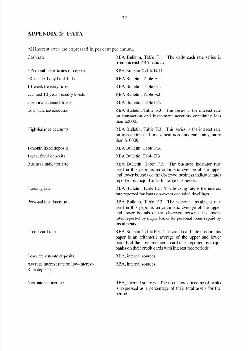
All interest rates are expressed in per cent per annum.

Cash rate RBA Bulletin, Table F.1. The daily cash rate series is

from internal RBA sources.

3-6-month certificates of deposit RBA Bulletin, Table B.11.

90 and 180-day bank bills RBA Bulletin, Table F.1.

13-week treasury notes RBA Bulletin, Table F.1.

2, 5 and 10-year treasury bonds RBA Bulletin, Table F.2.

Cash management trusts RBA Bulletin, Table F.4.

Low-balance accounts RBA Bulletin, Table F.3. This series is the interest rate

on transaction and investment accounts containing less

than $2000.High-balance accounts RBA Bulletin, Table F.3. This series is the interest rate

on transaction and investment accounts containing more

than $10000.

1-month fixed deposits RBA Bulletin, Table F.3.

1-year fixed deposits RBA Bulletin, Table F.3.

Business indicator rate RBA Bulletin, Table F.3. The business indicator rate

used in this paper is an arithmetic average of the upper

and lower bounds of the observed business indicator rates

reported by major banks for large businesses.

Housing rate RBA Bulletin, Table F.3. The housing rate is the interest

rate reported for loans on owner occupied dwellings.

Personal instalment rate RBA Bulletin, Table F.3. The personal instalment rate

used in this paper is an arithmetic average of the upper

and lower bounds of the observed personal instalment

rates reported by major banks for personal loans repaid by

instalments.

Credit card rate RBA Bulletin, Table F.3. The credit card rate used in this

paper is an arithmetic average of the upper and lower

bounds of the observed credit card rates reported by major

banks on their credit cards with interest free periods.

Low-interest-rate deposits RBA, internal sources.

Average interest rate on low-interest- RBA, internal sources.

Rate deposits

Non-interest income RBA, internal sources. The non interest income of banks

is expressed as a percentage of their total assets for the

period.



33

Operating expenses RBA, internal sources. The operating expenses are

expressed as a percentage of banks total assets for the

period.

Charge to profit by banks for bad and RBA, internal sources. The charge to profit is expressed

doubtful debts as a percentage of loans and acceptances. It is anaggregate for the major banks. The data are based on

reports published by banks at the end of their financial

years. For most banks these reports are published at end

September. One bank's financial year ends in June.



34

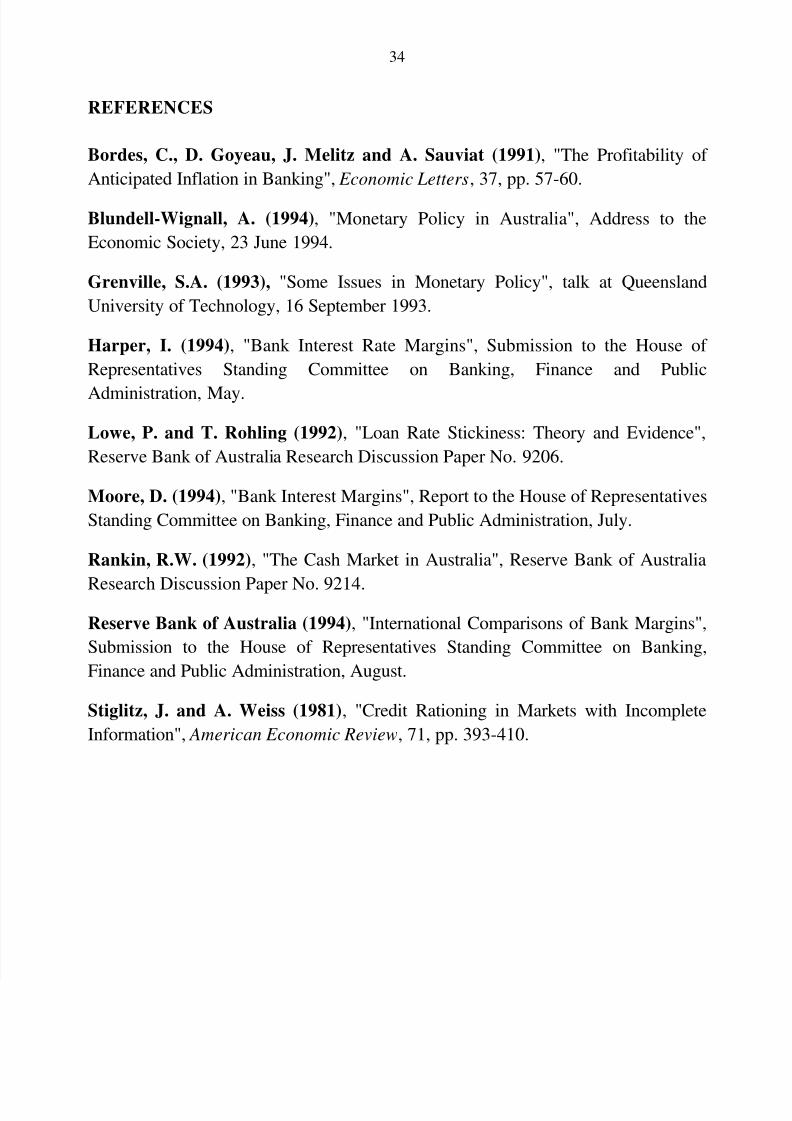
REFERENCES

Bordes, C., D. Goyeau, J. Melitz and A. Sauviat (1991), "The Profitability of

Anticipated Inflation in Banking", Economic Letters, 37, pp. 57-60.

Blundell-Wignall, A. (1994), "Monetary Policy in Australia", Address to the

Economic Society, 23 June 1994.

Grenville, S.A. (1993), "Some Issues in Monetary Policy", talk at Queensland

University of Technology, 16 September 1993.

Harper, I. (1994), "Bank Interest Rate Margins", Submission to the House of

Representatives Standing Committee on Banking, Finance and Public

Administration, May.

Lowe, P. and T. Rohling (1992), "Loan Rate Stickiness: Theory and Evidence",

Reserve Bank of Australia Research Discussion Paper No. 9206.

Moore, D. (1994), "Bank Interest Margins", Report to the House of Representatives

Standing Committee on Banking, Finance and Public Administration, July.

Rankin, R.W. (1992), "The Cash Market in Australia", Reserve Bank of Australia

Research Discussion Paper No. 9214.

Reserve Bank of Australia (1994), "International Comparisons of Bank Margins",

Submission to the House of Representatives Standing Committee on Banking,

Finance and Public Administration, August.

Stiglitz, J. and A. Weiss (1981), "Credit Rationing in Markets with Incomplete

Information", American Economic Review, 71, pp. 393-410.

Documents

Relation Between Cash Rate