REIT Capital Budgeting and Equity Marginal Q*

Brent W. Ambrose The Pennsylvania State University

and

Dong Wook Lee

Korea University Business School

April 23, 2008

Abstract

Equity marginal q is the change in market value of a company’s equity in conjunction with a one-unit unexpected change in its asset base. Hence, it is a profitability index that evaluates a firm’s capital budgeting decisions at the margin. In this paper, we estimate the equity marginal q for real estate-managing public corporations, namely, real estate investment trusts (REITs), in an attempt to understand how the various costs and benefits of being a public corporation play a role in managing this important asset class. After controlling for equity issuance and leverage that can mechanically affect the equity marginal q ratio, we find that REITs with greater idiosyncratic volatility and higher stock turnover have a higher equity marginal q, confirming the information and liquidity benefits of public stock markets. In addition, the holdings of institutional investors and their investment horizons are respectively positively related to equity marginal q, suggesting that monitoring power is attributable mostly to institutions with a long-term perspective. Finally, firm size is found to be negatively related to equity marginal q. Keywords: real estate investment trusts (REITs); capital budgeting; equity marginal q ratio * This study is funded by the Real Estate Research Institute (RERI) 2007 research grant. Dong Wook Lee also acknowledges the financial support from the Asian Institute of Corporate Governance at Korea University Business School. We are grateful to Jim Clayton and Jim Shilling for their valuable comments and suggestions. Any remaining errors are our own.

1. Introduction

Real estate is an important asset class in the economy. Not only does real estate account for a

large fraction of the national wealth and consumption (Mills 1987; Hendershott 1989), but

investing in real estate is also known to lead the business cycle (Green 1997). Reflecting real

estate’s importance in the economy, many investors also utilize this asset class as a portfolio

diversification tool due to its low correlation with other assets. Consequently, it is crucial to

understand how real estate is invested and managed in the economy.

Given the nature of real estate and real estate investment, its ownership by public

corporations (REITs) has both advantages and disadvantages. On one hand, as real estate entails

large fixed investment, public corporations may have an advantage over private peers through

better access to capital. Furthermore, equity trading in public markets may provide valuable

managerial information and foster its production. In addition, REITs offer a readily transferable

ownership interest in real estate. On the other hand, however, various agency problems inherent

in a public company can create adverse effects. Related, it is also possible that investing in real

estate requires area-specific information that is subtle and hard to communicate by nature: A large

public corporation may not be as efficient as its private peer in dealing with this type of

information.

Consequently, we examine the efficiency of REIT investment in real estate properties. For

public corporations, a relatively precise measure of investment efficiency is available because the

value of the company is determined and observed in the public securities market. More precisely,

by examining the change in market value of those securities in conjunction with a one-unit

unexpected change in the REIT asset base, one can measure how outside investors weigh the

return on their investment in REITs against the return on their alternative investment

opportunities such as direct private investment in real estate. Recognized as the marginal q ratio

by Durnev, Morck, and Yeung (2004; DMY hereafter), this metric is the profitability index of the

marginal investment from the perspective of outside capital providers. In this paper, we

1

particularly focus on equity capital providers by positing an equity-maximizing firm with long-

term debt outstanding.1 Specifically, we estimate the equity marginal q ratio for REITs, and

associate our estimates with various proxies for the costs and benefits of being a public company

in managing assets.

Several unique features of REITs justify our application of equity marginal q. First, REITs

are subject to a mandatory payout policy (at least 90% of earnings) and, in return, avoid paying

corporate tax. It thus follows that REITs raise capital externally and at the same time have fewer

reasons to use debt or prefer it to equity. Therefore, it is instructive to examine how equity value

changes in response to investment decisions. This also alleviates the problems that arise from the

lack of market value information for debt securities.

The absence of corporate tax also makes investment decisions more transparent. In general,

one important consideration in the capital budgeting process is the marginal tax rate – i.e., how

much tax liabilities increase for a one-dollar extra profit from a new project. Unfortunately, the

marginal tax rate is not observable to researchers, so they have difficulty understanding exactly

how corporate managers take into account these tax effects (see, e.g., Graham and Mills 2007).

With REITs, however, this is not an issue, since REITs do not pay corporate tax. Moreover, the

fact that REIT assets are traded (albeit infrequently) in the secondary market and thus their value

is observed with relatively greater precision also contributes to the transparency of REIT

investment decisions.

It is also noteworthy that since 1990 the U.S. REIT sector has been mostly in a growth stage,

suggesting that over-investment could be a potential concern. This observation warrants a

marginal, rather than average, metric for an investment efficiency measure. It also facilitates the

interpretation of equity marginal q, since growth options justify a q ratio that is higher than one

(or other optimal level). In other words, the joint-hypothesis problem is significantly mitigated

1 For example, Henessy (2004) postulates the same corporate goal.

2

with REITs. Finally, focusing on this particular industry allows us to utilize the rich firm-level

dispersion, while controlling for various (and often unknown) industry-level characteristics.

Using the universe of equity REITs listed on the NYSE, AMEX, or Nasdaq for the period

from 1993 to 2005, we find that the equity marginal q ratio for the REIT sector is of the order of

0.45, meaning that a one-dollar unexpected increase in asset base is associated with a 45-cent

increase in the market value of equity. Before making any inference, we need to take into

consideration several mechanical factors affecting our estimation. First, leverage will likely bias

downward the equity marginal q ratio, since an increase in corporate assets first accrues to debt

holders before contributing to equity value. Second, equity issuance activities may affect our

estimates as we use the total, not per-share, market value of equity. Finally, it should be noted

that REITs, at the time of going public, can record their properties either at the then current value

or at the historical value, creating a situation in which two otherwise identical REITs have

different book asset values. Although not necessarily a bias in a certain direction, this noise will

be particularly stronger among young REITs whose asset values are still affected by their asset-

recording decision upon IPO.

Analysis of the sub-samples sorted by leverage, equity issuance, or post-IPO age reveals that

equity issuance, and firm age to a weaker extent, are positively related to equity marginal q. In

contrast, leverage does not appear to affect our q estimates. The lack of a leverage effect is in

fact reasonable given the known efforts of REITs to maintain their target capital structure by

issuing equity when they have more debt (e.g., Brown and Riddiough 2003): that is, high leverage

REITs are subject to two countervailing effects on their equity marginal q.

When we examine the temporal variation in the sector’s equity marginal q ratio, we find that

it is mostly explained by the sector’s equity issuance activities, its growth opportunities, and the

general bond market condition as measured by the credit risk premium. Additionally, although

we find a significantly lower equity marginal q for diversified REITs, their time-varying presence

does not explain the time-variation in the sector’s equity marginal q ratio.

3

After examining the time-variation and the mechanical forces behind the marginal equity q,

we begin our in-depth analysis of the estimated equity marginal q ratio by associating it with

various proxies for the costs and benefits of being public. We find that the equity marginal q at

the individual firm level (i.e., individual deviations from the sector average) is correlated with the

proxies for the signaling and monitoring mechanisms of public stock markets. First of all, firm-

specific stock return volatility, a common proxy for private information produced in the stock

market, is found to be positively related to equity marginal q. This variable is motivated on the

grounds that private information held by informed traders tends to be firm-specific rather than

market- or industry-wide, and thus a greater contribution of firm-specific shocks to stock return

volatility indicates greater presence of informed traders (e.g., Durnev, Morck, and Yeung 2004).

Our finding is hence consistent with public stock markets helping managers make better

investment decisions by providing managerial information such as the cost of equity capital

(Chen, Goldstein, and Jiang 2007). The liquidity benefit of a public company is also confirmed,

since the stock turnover is positively related to equity marginal q.

Institutional ownership is similarly positively related to equity marginal q, consistent with the

finding of Harzell, Sun, and Titman (2006) that institutions play a monitoring role. Perhaps more

important, the investment horizon of the institutional investors is also positively related to equity

marginal q, implying that the beneficial monitoring stems mostly from institutions with a long-

term perspective. Finally, larger firm size is associated with a lower equity marginal q.

To more directly address the counter-argument that the observed equity marginal q for the

sector is at the optimal level and thus any deviation from it should be viewed as a sign of

inefficient capital budgeting decisions, we examine the deviation squared rather than the

deviation itself. Our results further make this counter-argument implausible, as the estimated

coefficients lead to a disturbing interpretation. For example, institutional ownership is positively

related to the deviation squared, which would have to be interpreted as having more institutions

as equity holders being associated with a poorer investment decisions.

4

In summary, our analysis shows that managing real estate in a public corporation is beneficial

under some conditions. More precisely, information emerges as an important consideration, and

a good governance system should be in place to mitigate the agency problems. We also find it

crucial to engage equity holders with a long-term perspective. This latter implication will be

particularly important given the long-lived nature of real estate properties.

This paper proceeds as follows. In the next section, we detail our sample and data. Section 3

first provides the theoretical background of equity marginal q and then reports the equity

marginal q estimate for the REIT sector along with a discussion of the associated estimation

issues. Section 4 examines the time-series patterns of the sector marginal q ratio, and conducts

the cross-sectional analysis using the individual firm level data. Finally, Section 5 concludes the

paper.

2. Sample and data

To construct the sample, we begin with all equity REITs ever listed on the NYSE, AMEX, or

Nasdaq between 1993 and 2005, as identified by the CRSP/Ziman database. In order to be

included in the analysis, we require each REIT to have at least 45 weekly stock returns on CRSP

for a given year, along with the accounting data from Compustat needed for marginal q

estimation.2 Finally, we exclude firm-year observations whose annual change in gross asset (the

sum of total assets and depreciation) is greater than 300 percent.3 The first line of Table 1 reports

the number of REITs in our sample. The maximum number of REITs in a given year is 181, and

no year has fewer than 104. Typically, we have 155 REITs during a year.

2 As an alternative to using the accounting book value of assets, we use the net asset value from a different data source, namely the SNL database. These results are discussed in Section 3.2. 3 Truncation of extreme observations is also found in other studies. For example, Gentry and Mayer (2003) and Hartzell, Sun, and Titman (2006) eliminate the observations whose annual asset growth rate is greater than 100 percent. Our use of a higher cutoff (i.e., 300 percent) biases the estimated q ratio upwards by allowing for the stock price response to a larger asset value change. In Section 3.1, we report the marginal q estimates based on alternative truncation cutoff levels.

5

The second panel of Table 1 reports the summary statistics of the variables required for

estimating the equity marginal q. Specifically, Et is the closing stock price (#199) times the

number of shares outstanding (#25) in year t; At is total assets (#6) plus depreciation (#125) in

year t; and Dt is cash dividends (#127) plus stock repurchases (#115) in year t. The sample

statistics show that our marginal q estimates are not caused by extreme values of these variables.

The annual change in the market value of equity relative to the beginning-of-the-year gross total

assets (ΔEt/At-1) ranges from -55 percent to 174 percent with the mean of 14 percent. The ratio of

equity market value to total assets (Et-1/At-1) also shows no extreme values; it ranges from 5

percent to 209 percent with the mean value of 62 percent. Finally, disbursements to equity

holders account for approximately 6 percent of total assets.

3. Equity marginal q of REIT sector

3.1. Theoretical background of equity marginal q

DMY have the following definition of marginal q ratio:

][][1)1(

1010

PIECNPVE

rcfE

CKVq

tt

t =+=⎥⎥⎦

⎤

⎢⎢⎣

⎡

+=

ΔΔ

= ∑∞

=

& , (1)

where cft is the cash flows at t from the marginal project, C0 is its initial capital outlay, and r is

the risk-adjusted discount rate. The last term PI stands for the profitability index, and all the

expectations (denoted by E [.]) are from the perspective of outside investors. To estimate

marginal q, the authors rewrite the above equation as follows:

)ˆˆ1()ˆˆ1(

,,1,,

,,1,,

,1,

,1,,

δ tjtjtjtj

tjtjtjtj

tjttj

tjttjtj gAA

drVVAEAVEVq

−+−−+−

=−−

=−

−

−

−& , (2)

where V is the market value of firm j and A is its stock of capital goods. Et-1 is the expectation

operator at time t-1 (it does not represent equity), is the expected return from owning the

firm, is the disbursements to investors, is the expected rate of spending on capital

r tjˆ ,

d tjˆ , g tjˆ ,

6

goods, and is the expected depreciation rate on those capital goods. The authors obtain the

regression equation for marginal q estimation by cross-multiplying and simplifying the above

equation.

δ̂ ,tj

In equation (2), it is possible to use equity value only as the numerator if an equity-

maximizing corporate manager is assumed (DMY; p.75). Specifically, this alternative approach

implies:

)ˆˆ1()ˆˆ1(

,,1,,

,,1,,

,1,

,1,,

δ tjtjtjtj

tjtjtjtj

tjttj

tjttjtj gAA

drSSAEASESq

−+−−+−

=−−

=−

−

−

−& , (3)

where S denotes the market value of equity, and and are defined accordingly for equity,

not for equity plus debt. With similar cross-multiplications and simplifications, this equation is

equivalent to:

r tjˆ , d tjˆ ,

uAD

ASr

AAAqgq

ASS

tjtj

tjj

tj

tjj

tj

tjtjjjjj

tj

tjtj,

1,

,

1,

1,

1,

1,,

1,

1,, )( +++−

+−−=−

−−

−

−

−

−

− ξδ && (4)

or

uAD

AS

AA

AS

tjtj

tj

tj

tj

tj

tj

tj

tj,

1,

,2

1,

1,1

1,

,0

1,

, +++Δ+=Δ−−

−

−−

βββα , (5)

where Dj = Sj,t-1dj. Equation (5) shows that the coefficient for the asset change isolates the

marginal q from the perspective of equity holders.4

4 We also discuss Hennessy’s (2004) version of equity marginal q. By assuming a constant return to scale and a price-taking firm, he starts with firm-value average q, which is equivalent to firm-value marginal q with the two assumptions (see Hayashi 1982):

KKDKS

KQ0

000000

),(),(),( εεε+

≡ .

Hennessy shows the following relationship between average Q and equity’s marginal q:

KKR

KQKq0

000000

),(),(),( εεε −= ,

where the second term in the right-hand side represents the normalized current market value of total default recoveries (R). In other words, his version of equity marginal q is the market value of equity (S) plus some of the market value of debt (D – R), divided by the capital stock (K). To obtain this ratio at the margin without making the assumptions of constant return to scale and price-taking firm, we need to consider how

7

3.2. Equity marginal q estimates

To obtain the equity marginal q ratio, we employ the equation (5) (with some modification

suggested by Ferreira and Laux (2007)). Specifically for REITs, we estimate:

εβββα tjtj

tj

tj

tj

tj

tj

tj

tj

AD

AE

AA

AE

,1,

,2

1,

1,1

1,

,0

1,

, +++Δ+=Δ−−

−

−−

, (6)

where Ej,t is the market value of REIT j’s common equity at time t, Aj,t is the book value of the

gross total assets of REIT j at time t, and Dj,t is the cash dividends and repurchases of REIT j at

time t. The coefficient for ΔAt/ΔAt-1 (i.e., β0) corresponds to the estimated equity marginal q ratio,

that is, the change in equity market value in response to the contemporaneous one-unit

unexpected change in asset base. As detailed in the previous sub-section, the expected change in

asset value is lumped together with the marginal q in the intercept. The coefficient for Et/At-1 (i.e.,

β1) corresponds to the expected increase in equity. Finally, β2 reflects the impact of dividends on

changes in equity.

We estimate equation (6) via three methods to ensure robustness of our estimates. First, we

follow the Fama-MacBeth (1973) method by estimating the equation each year and then

averaging the yearly estimates over time (while adjusting the test statistics for the serial

correlation). Second, we estimate the equation as a panel with year fixed effects (i.e., 12 year

dummy variables) while allowing for correlations among observations from the same REIT.

Third, we estimate the equation as a pooled GLS with the White (1980) covariance estimator.

nS a d D – R change respectively in response to a one-unit change in K. In his model setup, D – R is

[ ]∫ −T rt dtbeE0

, where b is the periodic debt payment and T is the point in time when the firm goes

bankrupt. Consequently, D – R is not a function of K, and thus his version of equity marginal q without the two assumptions would be consistent with ours, which is:

KKS

KqΔ

Δ=

0

0000

),(),( εε .

8

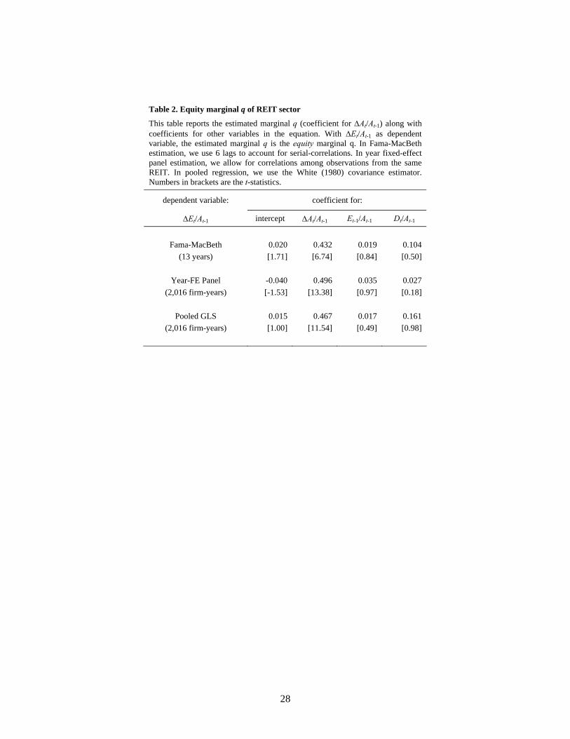
Table 2 reports the results. The Fama-MacBeth estimate for equity marginal q is 0.432,

meaning that for the one-dollar increase in REIT gross total assets at the margin, the equity

market value increases by 43.2 cents. This magnitude is robust across the three estimation

methods, as the panel estimate of the equity marginal q is 0.496 and its pooled GLS estimate is

0.467. All three marginal q estimates are statistically different from one (as well as from zero) at

the 1 percent level.5

The original argument by Tobin (1969) is that a less-than-one equity marginal q ratio implies

that the value of the marginal project from the perspective of equity holders is smaller than its

costs because the company has exhausted its positive-NPV projects and is now engaging in

negative-NPV projects (i.e., over-investment).6 Conversely, a higher-than-one equity marginal q

implies that equity value increases more than one dollar for the one-dollar investment at the

margin; hence, the company is under-investing. This interpretation, however, is not correct if the

marginal project is correlated with the company’s growth options and the equity value changes in

response to changes in these growth prospects. More specifically, as the numerator of the q ratio

includes the option value of the project as well as its cash flows, a higher-than-one q ratio can be 5 In an unreported result, the alternative cutoff level of 100 percent for annual total asset change yielded a much lower equity marginal q of 0.344 (Fama-MacBeth), 0.352 (panel), and 0.310 (pooled GLS) with a smaller sample of 1,908 firm-year observations over 13 years. With the cutoff level of 500 percent, the three estimation methods produced respectively 0.463, 0.566, and 0.536. Using the cutoff of 1,000 percent, we obtained the similar equity marginal q estimates between 0.440 and 0.499. Finally, without any cutoff, the panel and pooled GLS estimates were respectively 0.612 and 0.593, while the Fama-MacBeth estimate was 0.481. In an unreported result, we also used the net asset value, which is defined as the value of total assets minus total liabilities, and also includes property management and partnership incomes. Hence, this measure can correctly reflect the recent trend that several large REITs have entered the property management business on behalf of other investment companies such as pension funds. This asset management activity will not appear on the balance sheet (i.e. book value of assets) unless the REIT has a stake in the properties (or the delegating funds themselves). The cost of using the NAV is that the number of REITs is reduced almost by 30 percent. Such limited sample size is the typical cost of using the net asset value versus accounting book value. For example, Hartzell, Sun, and Titman (2006), while acknowledging the potential advantage of using the net asset value, use the accounting book value to maintain the breadth of their sample. They report that the correlation coefficient between net asset-based average q and book value-based average q is as high as 0.92. We found that the NAV-based equity marginal q ratio ranges from 0.138 to 0.311, which are lower than our book value-based q estimates. 6 This interpretation assumes that a manager takes projects in the order of their net present values. This assumption is not unrealistic even if one considers the agency problems associated with managerial discretion. As in Stulz (1990), perquisites enjoyed by managers are likely to increase with corporate resources, which will increase with the net present values of the projects that the manager takes.

9

consistent with efficient investment decision. In the next section, we discuss this consideration

and others affecting the optimal level of marginal equity q in greater detail.

Regarding the coefficient for Et/At-1 (i.e., β1), since we use the stock price changes net of the

disbursement, our estimates reflect the investor’s expected capital gain and equity issuance.

Across the three estimation methods, we find β1 to be between 0.017 and 0.035. Given the

substantial dividend payouts to REIT shareholders, the estimated increase in equity value of

approximately 2 percent to 3 percent per year is not unreasonable. For example, Capozza and

Seguin (2003) report that the annual capital gain is of the order of 2 percent.

Finally, the construction of equation (6) suggests that the coefficient for Dt/At-1 (i.e., β2)

should equal -1.0 in principle, since a one-dollar dividend mechanically reduces the stock price

by the same amount. However, as is noted by DMY, different tax brackets across REIT

shareholders may make this coefficient different from one. Uniquely, REITs also pay as much as

90 percent of their earnings as dividend and, as a consequence, frequently issue new equity.

Hence, our estimate is likely to be different from minus one. The signs of our coefficient

estimates for this variable turn out to be all positive, although they are not significant.

3.3. Estimation issues

3.3.1. Downward biases in equity marginal q

Several mechanical factors may affect the equity marginal q ratio. Among others, leverage

could introduce a downward bias, since debt holders have a senior claim on the firm’s assets. In

other words, any increase in corporate assets will accrue to equity holders only after debt holder

claims are satisfied; hence, it is possible that our seemingly low equity marginal q estimate

reflects the use of leverage by REITs. To understand the leverage effect, it is instructive to refer

to equation (1). In the original firm-value q ratio, the numerator represents the cash flows

accruing to all capital providers (i.e., equity holders and debt holders) discounted at the weighted

average costs of capital. It is a textbook result that this “firm value” is the same as the “equity

10

value” which is the cash flows accruing to equity holders discounted at the cost of equity capital,

as long as the default probability is zero. Intuitively, this is expected as the value of debt is

positively bounded, so any incremental cash flows belong to equity holders as long as the debt

payments are covered. As a result, as long as a non-zero default probability exists, the equity

marginal q will be lower than the firm-value marginal q. Also, its optimal level cannot be one;

instead, it should be below one (Hennessy 2004).

Another mechanical factor behind the equity marginal q is the equity issuance activities.

Note that we use the total market value of equity, as opposed to the per-share price, to estimate

equity marginal q. Consequently, an increase in the number of shares can mechanically raise the

q ratio even if the stock price does not change.

In fact, leverage and equity issuance are closely related. Prior studies have shown that REITs

maintain their target capital structure, meaning that greater equity is issued by high-leverage firms

(e.g., Brown and Riddiough 2003). Hence, on one hand, higher leverage represents a greater

claim by debt holders to corporate cash flows and thus reduces equity marginal q. On the other

hand, high leverage causes more equity to be issued, making the equity marginal q higher.

Finally, in estimating the equity marginal q, we rely on the accounting book value of assets.

REITs, at the time of going public, record their properties either at the then current value or at the

historical value, creating a situation in which two otherwise identical REITs have different book

asset values. For example, if the historical value is lower than the market value, then REITs that

recorded the IPO assets at historical value will have a lower asset base and thus a higher equity

marginal q. If the historical value is higher, then we would have the opposite result. In either

case, this effect will be more pronounced among young REITs, since their decisions at the time of

the IPO have the lingering effect on the book value of their assets.

To address the above three factors, we construct sub-samples sorted by leverage, equity

issuance, or post-IPO age, and examine whether equity marginal q is different in these

11

dimensions. Specifically, we estimate the following equation using leverage- or equity issuance-

sorted sub-samples:

εβββαα tjtj

tj

tj

tjk

hmkk

tj

tj

hmkkk

tj

tj

AD

AAD

AAD

AE

,1,

,2

1,

,

.,0

1,

,0

,1,

, ++Δ+Δ++=Δ−−=−=−

∑∑ , (7)

where Dk is the dummy variable for one of the three sub-sample k (either m (median) or h (high)).

In this specification, the “low” sub-sample serves as the baseline. In other words, β0 is the equity

marginal q for the low-leverage sub-sample, and (β0+β0,k) is the equity marginal q for the sub-

sample k (m or h). The test statistic associated with β0,k thus determines the statistical difference

in equity marginal q between the sub-sample k and the benchmark sub-sample. We do not have

such concern with post-IPO age-sorted sub-samples, so we estimate the following equation:

εββββαα tjtj

tj

tj

tj

tj

tjk

hmkk

tj

tj

hmkkk

tj

tj

AD

AE

AAD

AAD

AE

,1,

,2

1,

1,1

1,

,

.,0

1,

,0

,1,

, +++Δ+Δ++=Δ−−

−

−=−=−∑∑ . (8)

Table 3 reports β0, β0+β0,m, and β0+β0,h from the three estimation methods, along with the

number of REITs in each sub-sample and their average of the sorting variable. In the left panel of

the table, it is quite striking that the leverage ratio-sorted sub-samples show little difference in

their equity marginal q. Even though their leverage ratios are meaningfully different (24 percent,

45 percent, and 65 percent respectively for the low-, medium-, and high-leverage ratio sub-

samples), their equity marginal q ratios are relatively similar. Specifically, the low-leverage ratio

sub-sample has an equity marginal q ratio between 0.388 and 0.482, depending on the estimation

method. Similarly, the equity marginal q ratios for the medium- and high-leverage ratio sub-

samples are, respectively, between 0.475 and 0.508 and between 0.434 and 0.513.

The no-result for leverage-sorted sub-samples is likely to be due to the fact that high leverage

REITs issue more equity, undoing the leverage effect on equity marginal q. As in prior studies,

we confirm that leverage and equity issuances are positively correlated. Hence, the middle panel

reports the q ratio for the equity issuance-sorted sub-samples. We observe a clear difference in

equity marginal q between the sub-samples, especially between low- and high-issuance sub-

12

samples. This result not only confirms our conjecture of the equity issuance effect, but also helps

rationalize the leverage effect.

In the right panel, we report the results for age-sorted sub-sample. Although not as strong as

the issuance-sorted sub-samples, there is a difference in q ratio in the dimension of post-IPO age.

Specifically, older REITs seem to have a higher q ratio, emphasizing the need to control for firm

age in the subsequent analysis.

3.3.2. Optimal level of equity marginal q

It is typically assumed that the optimal marginal q is one. Applying this to equity marginal q

ratio, it means that the one-dollar marginal investment is worth just one dollar to equity holders,

making the profitability index unity. In practice, however, various complications can cause the

optimal level to deviate from one, besides the obvious effect of leverage. As detailed by DMY (p.

77), it is virtually impossible to consider all the complications ex ante and adjust the optimal level.

However, the authors identify several important complications including the role of taxes, the

aggregation of investment projects, and the impact of growth options.

First, we consider the effect of taxes. A company can retain and reinvest earnings, converting

dividends income into capital gains. In this case, the differential between income and capital gain

tax rates can affect both the optimal level of q and its empirical estimates. Using a capital gain

tax rate of 14 percent and a dividend tax rate of 33 percent and also assuming that the marginal

investor is tax-exempt half of the time, DMY estimate the tax effect to be approximately 1.15.7

In other words, if the estimated equity marginal q is, say, 0.8, then equity holders in fact perceive

the one-dollar marginal investment to be worth 92 cents (0.8 times 1.15). In addition, the optimal

level of marginal q is elevated to 1.15. With REIT, however, most of the cash flows accruing to

equity holders are in the form of dividends, so the differential tax rates will not be economically

important. 7 ½*1 + ½*[(1–0.14)/(1–0.33)] ⇔ 1.15.

13

Second, since we use the annual changes in total assets as a measure of investment, it is

possible that marginal and non-marginal projects are lumped together. As the company is likely

to take the projects with higher net present values first, this aggregation will inflate the estimated

marginal q. To illustrate, suppose that the marginal project has zero-NPV (i.e., marginal q is 1)

and the previous project had a slightly positive NPV (its marginal q is, say, 1.1). If we aggregate

the two projects, then our q estimate will be between 1 and 1.1, which is higher than the true

marginal q of 1. The implication is that our marginal q estimate is higher than the true marginal q

of the sector. Hence, this consideration alone would not allow us to argue that the REIT sector is

operating at its optimum.

Finally, stock market valuations may reflect changes in the value of growth options as well as

that of the marginal investment. This scenario is particularly plausible when the marginal project

(or aggregated investment projects) is correlated with future growth options. As a result, the

optimal marginal q level does not have to be one when growth options are present and their value

changes. Although it is generally unclear how this consideration affects the optimal level of the q

ratio and its empirical estimate, REITs uniquely allow us to conjecture the direction of the biases

associated with this option feature for the following two reasons. First, REITs have been mostly

in the growth stage. Second, due to irreversibility of real estate investment, growth option value

is particularly important in REIT valuation. Consequently, the optimal q ratio for the REIT sector

is likely to be higher than the case of regular, industrial firms.

In summary, it is generally assumed that there exists an optimal level of q (e.g., unity) and

any deviation from it indicates inefficient investment. This creates a joint-hypothesis problem,

since a researcher first has to find the optimal q level in spite of various real world complications.

REITs uniquely help avoid this joint-hypothesis problem, since the sector has been growing most

of the sample period and real estate investment, due to its nature, entails the option feature. For

example, a higher equity marginal q than the sector average can be interpreted as a healthy sign of

capital budgeting.

14

4. Sector-wide and firm-level analysis of equity marginal q of REIT sector

In this section, we first examine the time-series trend in the REIT sector equity marginal q.

Since we have a short time-series (13 years), the sector-wide temporal variation in equity

marginal q is not our main interest. However, an understanding of how it varies over time and

what factors affect such temporal changes is a prerequisite for our later analysis of equity

marginal q at the individual firm level. Following the sector-wide time-series analysis, we

introduce the cross-section dispersion, with emphasis on the effect of the signaling and

monitoring mechanisms of public stock markets on individual equity marginal q ratios.

4.1. Time-series and cross-sectional patterns of equity marginal q

To first detect time-trends, we estimate yearly marginal q ratios. Specifically, we estimate

equation (6) every year to obtain the year-specific equity marginal q ratio. In the left panel of

Table 4, the year-by-year equity marginal q ratio declines significantly from 0.840 at the

beginning of the sample period to 0.154 by 2000. It then rebounds somewhat by the end of the

sample period. The 2005 estimate of equity marginal q of 0.363 is, however, approximately less

than one half of its initial level.

In the right panel, we estimate the equity marginal q for each of the property types. Their

equity marginal q ratios are estimated through the panel and the pooled GLS versions of equation

(6) by adding the interactive terms between the dummy variables for each property focus and the

percentage changes in gross total assets.8 Interestingly, there is no meaningful (and statistically

significant) difference in equity marginal q across different property types. The only exception is

the group of diversified REITs whose q ratio is significantly lower than the sector average. It

may appear surprising that most property types have similar equity marginal q ratios. However,

8 We do not use the Fama-MacBeth method due to the limited number of observations within a year for each investment style or property type.

15

our results can be interpreted that there are no arbitrage opportunities as different property types

are similarly profitable at the margin.

As discussed in the previous section, there are at least three variables that can potentially

explain the observed time-variation of the sector’s equity marginal q ratio. One is the growth

opportunities of the REIT sector, since the equity marginal q will reflect the option value as well

as the cash flows from the marginal project. Another factor is the equity issuance activity,

because it mechanically increases the number of shares (and thus the total market value of equity

assuming no change in the per-share price). The third one is the credit quality of the REIT sector,

as it represents the default likelihood (which reduces the equity marginal q ratio for the sector).

We construct each of the three variables at the sector level. Specifically, the growth

opportunity and equity issuance are respectively the cross-sectional averages of the lagged equity

market value scaled by lagged assets and of the individual equity issuances. For credit quality,

unfortunately only a few REITs have this information available. However, Brown and Riddiough

(2003) show that the REIT bond market is integrated into the broader bond market. Based on this

finding, we use the credit risk premium at the general bond market level (Moody’s Baa yield in

excess of 10-year Treasury yield) as a proxy for REIT sector credit quality. In addition to these

three variables, we include the number of diversified REITs, since we observed that they have a

significantly lower equity marginal q. Hence, it is possible that some of the time-variation is

attributable to the varying presence of diversified REITs.

Before proceeding further, we stress, again, that we do not attempt to make any meaningful

inference from our results, since there are only 13 observations. Instead, we just want to make

sure that we have an understanding of the temporal variation in equity marginal q during the

sample period, so that we can focus on firm-level variation in the subsequent analysis without

missing information in other dimensions.

The first panel of Table 5 reports the correlation coefficients between the four variables. As

might be expected, the credit risk premium, albeit obtained from the general bond market, is

16

significantly and negatively correlated with the growth opportunity variable. Other correlations

are not significant, except for those with the number of diversified REITs; this variable is

significantly correlated with all other three variables.

In the second panel, we estimate a regression of year-by-year sector q ratios (those that are

reported in the left panel of Table 4) on the above variables. Consistent with Table 3 results, the

equity issuance variable enters the regression with a positive and significant coefficient. Growth

opportunities, measured at the beginning of a given year, are also positively related to equity

marginal q that is estimated during the year. The credit default premium is negatively, albeit

statistically marginally, related to the sector’s q ratio, confirming that role of default likelihood in

determining equity marginal q ratio. Given the small number of observations and only a few

explanatory variables, the R-squared is quite impressive. Across the four specifications, the R-

squared is around 50 percent. Hence, it seems to be justified that we focus on firm-level variation

as long as we control for equity issuance, growth opportunities, and credit quality.

4.2. Equity marginal q and public stock markets -- Variables

Public corporations and their (dis)advantage over the private peers is not a new research topic.

Back in the 1980s, going private transactions (leveraged buyouts) triggered numerous studies ,

and the recent de-listings and privatization led by private equity funds has re-ignited this line of

research. Augmented with the IPO studies, we now have a good theoretical guidance for the

costs and benefits of being a public corporation (e.g., Bharath and Dittmar 2007; Boot, Gopalan,

and Thakor 2006). We thus build on those studies to identify proxies for the costs and benefits of

being public that are suited for REITs.

Bharath and Dittmar (2007) show that information and liquidity are two most important

considerations in remaining public (i.e., not choosing to be private), and they are particularly

relevant for REITs. Regarding information, it is well documented that uncertainty plays an

important role in real estate investment due to its irreversibility and “delayability” (Holland et al.

17

2000). Hence, information generated outside the company will help make sound capital

budgeting decisions by resolving uncertainty associated with real estate investment. Here, the

relevant information is the one that is not held by corporate manager. Based on this discussion,

we first employ the idiosyncratic stock return volatility, defined as 1 – R2. We obtain the R2 from

the year-by-year regression of the weekly stock returns of individual REITs on the value-

weighted portfolio of common (i.e., non-REIT) stocks and the value-weighted portfolio of all

sample REITs.9 This variable represents the proportion of REIT stock returns that is not

explained by the general stock market-wide or the REIT sector-wide shocks. It is also equivalent

to the volatility of the regression residuals divided by the volatility of the REIT stock returns.

Recent studies establish this variable as a measure of the amount of private information generated

in the stock market (e.g., Durnev, Morck, and Yeung 2004; Chen, Goldstein, Jiang 2007). The

rationale is that private information held by informed traders tends to be firm-specific rather than

market- or industry-wide; consequently, a greater contribution of firm-specific shocks to stock

return volatility can indicate greater participation of informed traders and thus greater amount of

their private information in the stock price.

Institutional ownership can be another proxy for information. At the same time, however, it

will gauge how much monitoring is at work for the corporate manager. As public corporations

naturally have diffused ownership (oftentimes held by uninformed, passive investors) and thus

are subject to agency problems associated with managerial discretion, institutional investors can

exert monitoring power and help improve the governance of REIT management (Hartzell, Sun,

and Titman 2006). Along this line, we also include insider ownership as measured by the

company common shares held by the top executives (CEO, CFO, COO, and presidents).

A related issue is the investment horizon of equity holders, because their horizons have an

impact on the managerial horizon and thus the investment decisions (e.g., Shleifer and Vishny

9 At least 45 weekly returns are used for this yearly regression, since we already screen the sample using this requirement.

18

1990). Recently, Gaspar, Massa, and Mantos (2004) devise a measure of investor short-termism

using the institutional holdings data, and find that their short-termism measure is related to the

frequency and premium of corporate takeovers in the U.S. We thus borrow their measure to see

whether investor horizon is related to equity marginal q ratio of REITs. Given the long-lived

nature of real estate properties, this horizon issue is potentially important.

Regarding liquidity, we use the daily average of stock turnover. In general, a public

corporation is desirable due to its readily transferable ownership. This benefit will be particularly

useful if the assets managed by the company are otherwise hard to access but an exposure to them

is valuable. Real estate properties meet these two conditions, and thus the liquidity of REITs will

be one important determinant of the evaluation of REIT investments by equity holders. We also

use the bid-ask spread of REIT stock prices as another liquidity measure. However, this variable

can also be interpreted as a measure of the efficiency in REIT stock valuation. As a widely

accepted proxy for information asymmetries among investors, a stock with a smaller bid-ask

spread can be considered to have a more reliable stock price that is closer to its fundamental value.

Along with the stock market-related firm characteristics, we control for leverage and debt

maturity. Viewed as a call option on corporate cash flows, equity value will be affected by the

debt amount and its maturity. We thus include these two variables in the firm-level analysis. For

the maturity variable, the limited data availability forces us to only calculate the fraction of total

debt that is due in more than one year. As discussed earlier, equity value as a call option on

corporate cash flows is particularly sensitive to the default probability, so we need to include the

credit quality for individual REITs. Unfortunately, this information is only scantly available. As

an alternative, we use a variable that is commonly used for credit rating decision, namely, interest

coverage ratio as measure by: (net income + depreciation and amortization + interest expenses) /

(interest expenses + preferred dividends).

19

Finally, we include firm size, post-IPO age, and a dummy variable for diversified REITs.

Since REIT size has increased significantly over time, we scale it by the inflation index (base

year: 1992).

4.3. Equity marginal q and public stock markets -- Summary statistics

Table 6 reports the above variables, along with the firm-level equity marginal q. It is difficult

to directly estimate the firm-level equity marginal q ratio, so we follow Ferreira and Laux (2007)

by using the individual deviations from the sector marginal q as a measure of individual marginal

q. Specifically, we use the residuals from the pooled GLS version of equation (6) as a measure of

equity marginal q at the individual firm level.10

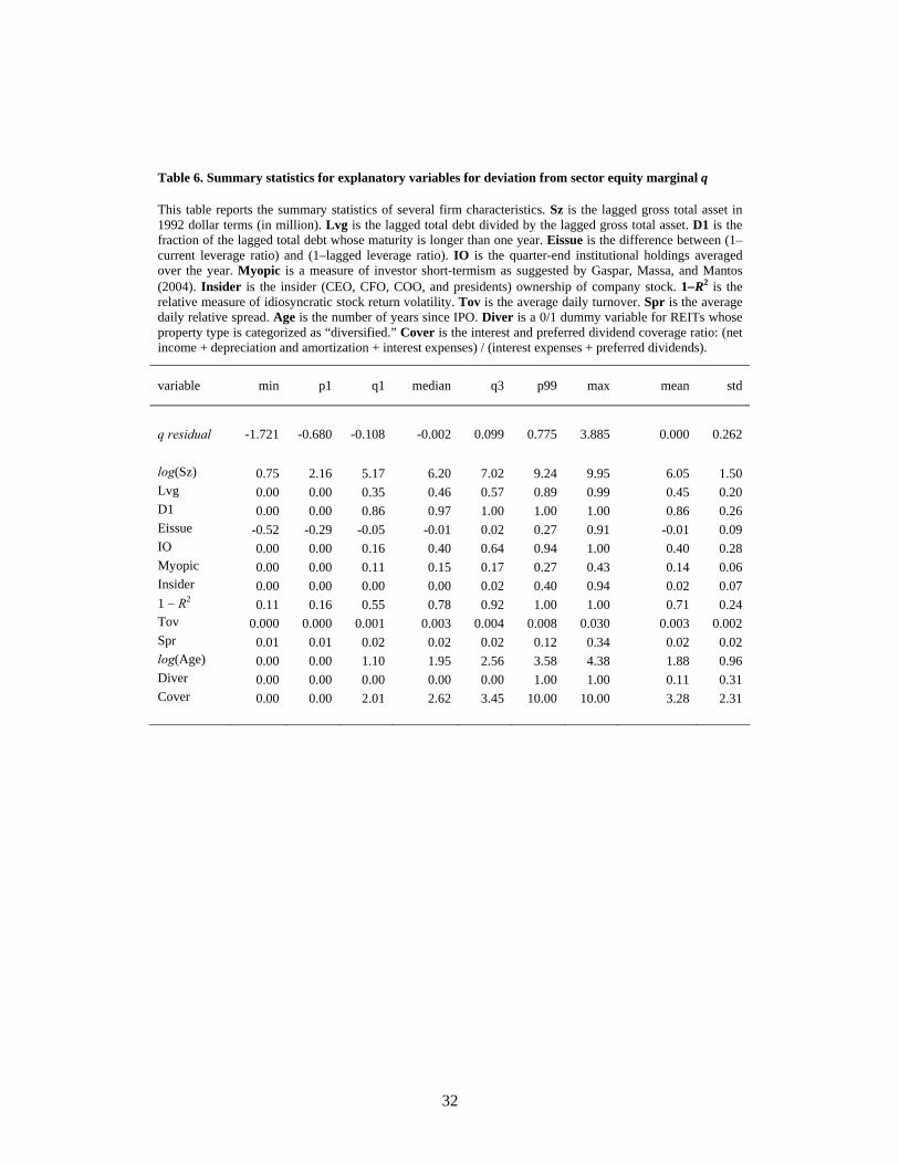
The first line of Table 6 reports the residuals from the sector equity marginal q estimation.

By construction, the mean value of the residuals is zero. However, they have extreme values at

both ends: the minimum value is -1.721 and the maximum is 3.885. To prevent these outliers

from affecting our results, we truncate the residuals at the 1st and the 99th percentiles;

consequently, the residuals used in the second-step regression range from -0.680 to 0.775.

Summary statistics of other variables are also reported in Table 6. For leverage, institutional

ownership, and insider ownership, we treat as missing if the value is greater than one. The

coverage ratio cannot be calculated when the company has no debt and does not pay any

preferred dividend (note that some of our sample REITs have no debt.) Thus, we winsorize this

variable at 10. Also, we winsorize it at 0 for REITs that have negative earnings.

Table 7 reports the correlation coefficient between the variables. Not surprisingly, most of

them are highly correlated. Among them, leverage and coverage ratio have a correlation

coefficient as high as -0.675, so having them together in one regression can be problematic.

Similarly, firm size is highly correlated with many of other firm characteristics. Hence, we will

10 We do not use the year fixed-effect panel method, since we want to directly observe and control for the time effects.

20

examine whether the regression coefficients are sensitive to including firm size. We additionally

attempt to mitigate the multicollinearity by first estimating the univariate regressions.

4.4. Equity marginal q and public stock markets -- Analysis

Table 8 reports the univariate regression results. As mentioned earlier, this is to address the

potential multicollinearity due to high correlation between the variables. However, the univariate

results should be interpreted with caution, since the true effect of a certain variable can be

isolated only when the effects of other variables are correctly controlled for.

Of the 13 variables that we initially consider, leverage, insider ownership, bid-ask spread, and

the dummy for diversified REITs do not appear promising. The p-values of the coefficients for

those variables, all based on the White (1980) covariance estimator, range from 0.377 to 0.958.

In contrast, equity issuance, investor short-termism, turnover, age, and coverage ratio are highly

significantly related to equity marginal q ratio at the individual firm level. Frm size, debt

maturity, institutional ownership, and idiosyncratic volatility are marginally significantly related

to equity marginal q ratio.

The coefficient sign for each of the variables is intuitive. A positive coefficient for equity

issuance is expected, as it increases the number of shares and thus raises the equity marginal q

ratio. The investor short-termism measure carries a negative coefficient, meaning that institutions

with a short-term perspective have an adverse effect on capital budgeting decisions. Stock

turnover is positively related to equity marginal q, confirming the liquidity benefit of being public.

Coverage ratio enters the regression with a positive sign, since a greater value for this variable

means a lower likelihood of default (i.e., greater cash flows accruing to equity holders and thus a

higher equity marginal q). A weakly negative coefficient for firm size suggests that larger REITs

over-invest compared to their smaller peers. A negative coefficient for debt maturity means that

REITs with short-term debt make better investment decisions. Finally, a positive coefficient for

21

institutional ownership and idiosyncratic volatility implies that there is a monitoring effect and

that information generated in stock markets helps managers make good investment decisions.

Table 9 reports the multivariate regression results. In Model (1), the variables that were

significant in the univariate regression continue to be significantly related to equity marginal q.11

In addition, institutional ownership and idiosyncratic volatility dramatically increase their

statistical significance with the same positive coefficient. When firm size is added (Model (2)),

the coefficients for other variables hardly change, and firm size itself enters the regression with a

significant and negative coefficient. These variables combined explain about 21 percent of the

variation of the dependent variable.

To better understand in which dimension those variables have the explanatory power, we

employ three more specifications. As noted at the bottom of the table, we first introduce firm

fixed effects to focus on the explanatory power of the variables for the within-firm variation. We

then replace the firm fixed effects with year fixed effects to turn our attention to within-year,

cross-sectional variation. Finally, we include both sets of fixed effects as the final regression

specification.

Comparing Models (3) and (4), we find that idiosyncratic volatility, stock turnover, and firm

age explain the within-firm variation, but not the within-year, cross-sectional dispersion of equity

marginal q ratios. In contrast, coverage ratio only explains the within-year variation. Firm size,

equity issuance, institutional ownership, and investor short-termism are significantly related to

equity marginal q in both specifications. Finally, Model (5) includes both firm and year fixed

effects, so that the coefficients are estimated based on the entire firm-year observations while

their firm- or year-specific effects are taken into account. In this specification, firm size and the

investor short-termism measure continue to be negatively related to equity marginal q. Equity

11 In estimating the multivariate regressions, we drop several variables that are not significant univariately but are highly correlated with other potentially useful variables. Specifically, we choose to drop leverage and debt maturity due to its correlation with the coverage ratio. Firm size is highly correlated with most of other variables, so we estimation two specifications, one with firm size and the other without.

22

issuance and institutional ownership also maintain their statistical significance with a positive

coefficient. However, idiosyncratic volatility and stock turnover become only marginally

significant, suggesting that they explain the time-series change in equity marginal q for a given

REIT.12

5. Conclusions

In this paper, we estimate the equity marginal q ratio for the REIT sector to examine whether

the REIT capital budgeting decisions are well aligned with the interests of shareholders. In

particular, we examine how the various signaling and monitoring mechanisms of public stock

markets are related to the degree of such alignment. REITs are a good setting for this

investigation since the type of assets under their management, namely, real estate properties,

allow for a more precise estimate for asset value and thus for q ratio. In addition, since REITs are

publicly traded securitization vehicles for assets that are important in asset allocation and

portfolio diversification, the results have the potential to provide broader implications for the

portfolio choice problem.

Our analysis shows that the equity marginal q at the individual firm level (i.e., individual

deviations from the sector average) is correlated with the proxies for the signaling and monitoring

mechanisms of public stock markets. Specifically, after controlling for equity issuance and

leverage that can mechanically affect the equity marginal q ratio, we find that REITs with greater

idiosyncratic volatility and higher stock turnover have a higher equity marginal q, confirming the

information and liquidity benefits of public stock markets. In addition, the holdings of

institutional investors and their investment horizons are respectively positively related to equity

12 In an unreported result, we examined the deviation squared in an attempt to more directly address the counter-argument that the observed equity marginal q for the sector is at the optimal level and thus any deviation from it should be viewed as a sign of inefficient capital budgeting decisions. We found that most of our variables preserve the sign of their coefficient and oftentimes lead to disturbing interpretations. For example, institutional ownership is positively related to the deviation squared, which would have to be interpreted as having more institutions as equity holders being associated with a poorer investment decision.

23

marginal q, suggesting that monitoring power is attributable mostly to institutions with a long-

term perspective. Finally, firm size is found to be negatively related to equity marginal q.

24

References

Bharath, S. and A. Dittmar, 2007, Why do firms use private equity to opt out of public markets? Journal of Finance, forthcoming.

Boot, Arnoud, Radhakrishnan Gopalan, and Anjan V. Thakor, 2006, The Entrepreneur's Choice between Private and Public Ownership, Journal of Finance, forthcoming.

Brealey, Richard, Stewart Myers, and Franklin Allen, 2006, Corporate Finance, 8th ed., McGraw-Hill.

Brown, D. and T. Riddiough, 2003, Financing choice and liability structure of real estate investment trusts, Real Estate Economics, 313-346.

Capozza, D. and P. Seguin, 2003, Special Issue: Real estate investment trusts—Foreword form the guest editors, Real Estate Economics, 305-311.

Chen, Qi, Itay Goldstein, and Wei Jiang, Price Informativeness and Investment Sensitivity to Stock Price, Review of Financial Studies, May 2007; 20: 619 - 650.

Durnev, Art., Randall Morck, and Bernard Yeung, 2004, Value-Enhancing Capital Budgeting and Firm-specific Stock Return Variation, Journal of Finance, 65-105.

Durnev, Art., Randall Morck, and Bernard Yeung, 2004, Value-Enhancing Capital Budgeting and Firm-specific Stock Return Variation, Journal of Finance, 65-105.

Durnev, Art., Randall Morck, Bernard Yeung, and Paul Zarowin, 2003, Does greater firm-specific return variation mean more or less informed stock price?, Journal of Accounting Research, 797-836.

Fama, E., MacBeth, J., 1973, Risk, Return, and Equilibrium: Empirical Tests, Journal of Political Economy 71, 607-636.

Ferreira, Miguel and Paul Laux, 2007, Corporate Governance, Idiosyncratic Risk, and Information Flow, Journal of Finance 62 (2007), 951-989.

Gasper, José-Miguel, Massimo Massa, and Pedro Matos, 2005, Shareholder investment horizons and the market for corporate control, Journal of Financial Economics, 135-165.

Gentry, William and Christopher Mayer, 2003, What can we learn about investment and capital structure with a better measure of q?, Unpublished working paper, Columbia University.

Graham, J. and L. Mills, 2007, Using tax return data to simulate corporate marginal tax rates, NBER Working Paper No. W13709.

Green, R., 1997, Follow the leader: How changes in residential and non-residential investment predict changes in GDP, Real Estate Economics, 253-270.

25

Hartzell, Jay, Libo Sun, and Sheridan Titman, 2006, The effect of corporate governance on investment: Evidence from Real Estate Investment Trusts, Real Estate Economics, 343-376.

Hayashi, Fumio, 1982, Tobin’s marginal q and average q: A neoclassical interpretation, Econometrica, 213-224.

Hendershott, P., 1989, Comment on social returns to housing and other fixed capital, Journal of the American Real Estate and Urban Economics Association, 212-217.

Hennessy, Christopher, 2004, Tobin’s Q, debt overhang, and investment, Journal of Finance, 1717-1742.

Mills, E., 1987, Has the United States overinvested in housing?, Journal of the American Real Estate and Urban Economics Association, 601-616.

Shleifer. A. and R. Vishny, 1990, Equilibrium short horizons of investors and firms, American Economic Review, 148-153.

Stulz, René M., 1990, Managerial discretion and optimal financing policies, Journal of Financial Economics, 3-28.

Tobin, J., 1969, A general equilibrium approach to monetary theory, Journal of Money, Credit and Banking, 15-29.

White, H., 1980, A heteroskedasticity-consistent covariance matrix estimator and a direct test for heteroskedasticity, Econometrica, 817-838.

26

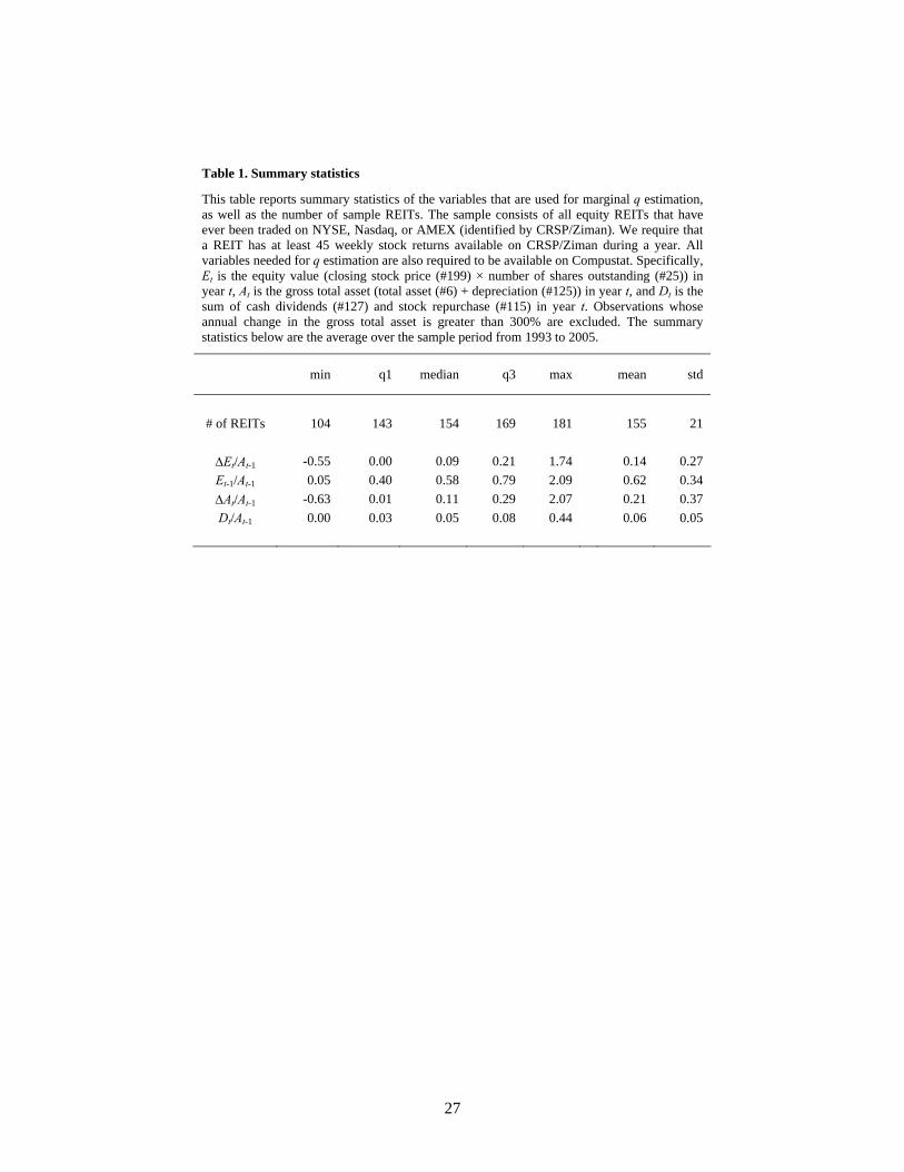
Table 1. Summary statistics

This table reports summary statistics of the variables that are used for marginal q estimation, as well as the number of sample REITs. The sample consists of all equity REITs that have ever been traded on NYSE, Nasdaq, or AMEX (identified by CRSP/Ziman). We require that a REIT has at least 45 weekly stock returns available on CRSP/Ziman during a year. All variables needed for q estimation are also required to be available on Compustat. Specifically, Et is the equity value (closing stock price (#199) × number of shares outstanding (#25)) in year t, At is the gross total asset (total asset (#6) + depreciation (#125)) in year t, and Dt is the sum of cash dividends (#127) and stock repurchase (#115) in year t. Observations whose annual change in the gross total asset is greater than 300% are excluded. The summary statistics below are the average over the sample period from 1993 to 2005.

min q1 median q3 max mean std

# of REITs 104 143 154 169 181 155 21

ΔEt/At-1 -0.55 0.00 0.09 0.21 1.74 0.14 0.27 Et-1/At-1 0.05 0.40 0.58 0.79 2.09 0.62 0.34 ΔAt/At-1 -0.63 0.01 0.11 0.29 2.07 0.21 0.37 Dt/At-1 0.00 0.03 0.05 0.08 0.44 0.06 0.05

27

28

Table 2. Equity marginal q of REIT sector

This table reports the estimated marginal q (coefficient for ΔAt/At-1) along with coefficients for other variables in the equation. With ΔEt/At-1 as dependent variable, the estimated marginal q is the equity marginal q. In Fama-MacBeth estimation, we use 6 lags to account for serial-correlations. In year fixed-effect panel estimation, we allow for correlations among observations from the same REIT. In pooled regression, we use the White (1980) covariance estimator. Numbers in brackets are the t-statistics.

dependent variable: coefficient for:

ΔEt/At-1 intercept ΔAt/At-1 Et-1/At-1 Dt/At-1

Fama-MacBeth 0.020 0.432 0.019 0.104

(13 years) [1.71] [6.74] [0.84] [0.50]

Year-FE Panel -0.040 0.496 0.035 0.027 (2,016 firm-years) [-1.53] [13.38] [0.97] [0.18]

Pooled GLS 0.015 0.467 0.017 0.161

(2,016 firm-years) [1.00] [11.54] [0.49] [0.98]

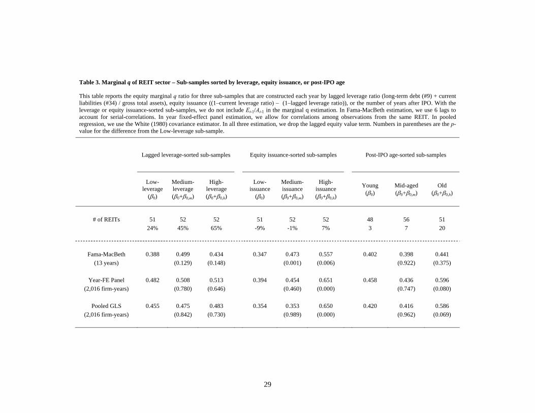
Table 3. Marginal q of REIT sector – Sub-samples sorted by leverage, equity issuance, or post-IPO age

This table reports the equity marginal q ratio for three sub-samples that are constructed each year by lagged leverage ratio (long-term debt (#9) + current liabilities (#34) / gross total assets), equity issuance ((1–current leverage ratio) – (1–lagged leverage ratio)), or the number of years after IPO. With the leverage or equity issuance-sorted sub-samples, we do not include Et-1/At-1 in the marginal q estimation. In Fama-MacBeth estimation, we use 6 lags to account for serial-correlations. In year fixed-effect panel estimation, we allow for correlations among observations from the same REIT. In pooled regression, we use the White (1980) covariance estimator. In all three estimation, we drop the lagged equity value term. Numbers in parentheses are the p-value for the difference from the Low-leverage sub-sample.

Lagged leverage-sorted sub-samples Equity issuance-sorted sub-samples

Post-IPO age-sorted sub-samples

Low-

leverage (β0)

Medium-leverage (β0+β0,m)

High-leverage (β0+β0,h)

Low-

issuance (β0)

Medium- issuance (β0+β0,m)

High- issuance (β0+β0,h)

Young

(β0) Mid-aged (β0+β0,m)

Old (β0+β0,h)

# of REITs 51 52 52 51 52 52 48 56 51

24% 45% 65% -9% -1% 7% 3 7 20

Fama-MacBeth 0.388 0.499 0.434 0.347 0.473 0.557 0.402 0.398 0.441 (13 years) (0.129) (0.148) (0.001) (0.006) (0.922) (0.375)

Year-FE Panel 0.482 0.508 0.513 0.394 0.454 0.651 0.458 0.436 0.596

(2,016 firm-years) (0.780) (0.646) (0.460) (0.000) (0.747) (0.080)

Pooled GLS 0.455 0.475 0.483 0.354 0.353 0.650 0.420 0.416 0.586 (2,016 firm-years) (0.842) (0.730) (0.989) (0.000) (0.962) (0.069)

29

Table 4. Equity marginal q by year or by property type

This table reports the estimated marginal q for the REIT sector by year and property type. For the year-by-year results, we estimate the equation each year. For the property type results, we utilize either the year fixed-effect model or the pooled GLS.

By year By property type

year OLS Property type Year-FE Panel

Pooled GLS

1993 (n=104) 0.840 Industrial/Office (n=43) 0.553 0.524 1994 (n=146) 0.294 Health Care (n=12) 0.445 0.399 1995 (n=181) 0.535 Lodging/Resort (n=12) 0.528 0.528 1996 (n=176) 0.686 Residential (n=27) 0.553 0.531 1997 (n=164) 0.727 Retail (n=38) 0.460 0.431 1998 (n=169) 0.260 Diversified (n=17) 0.234 0.199 1999 (n=180) 0.185 Unclassified (n=6) 0.498 0.384 2000 (n=166) 0.154 2001 (n=154) 0.569 2002 (n=143) 0.357 2003 (n=143) 0.475 2004 (n=142) 0.171 2005 (n=148) 0.363 Average 0.432 Average 0.496 0.467

30

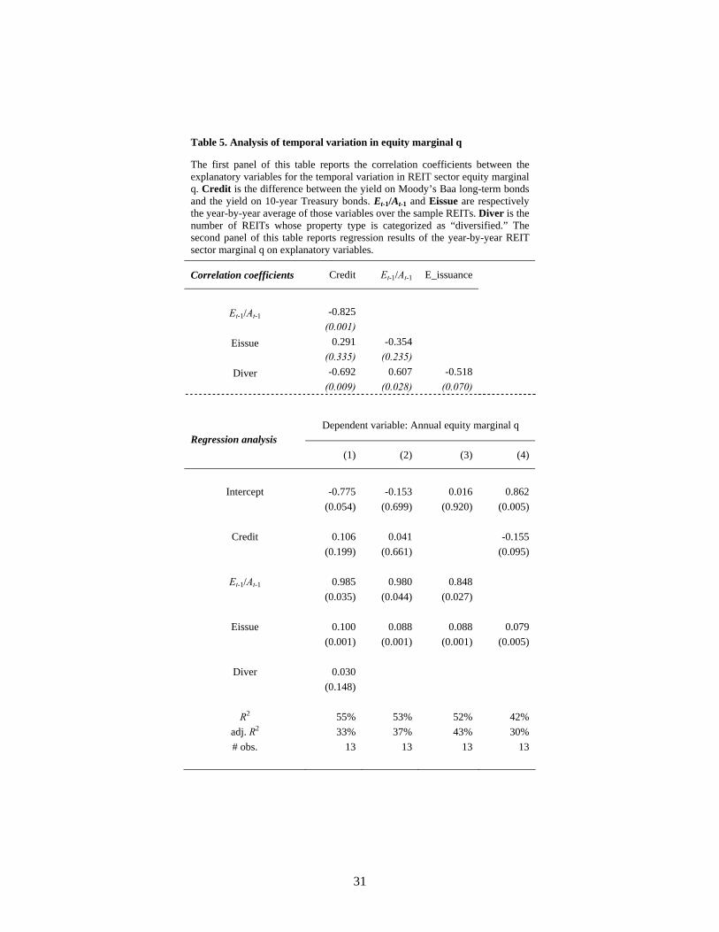
Table 5. Analysis of temporal variation in equity marginal q

The first panel of this table reports the correlation coefficients between the explanatory variables for the temporal variation in REIT sector equity marginal q. Credit is the difference between the yield on Moody’s Baa long-term bonds and the yield on 10-year Treasury bonds. Et-1/At-1 and Eissue are respectively the year-by-year average of those variables over the sample REITs. Diver is the number of REITs whose property type is categorized as “diversified.” The second panel of this table reports regression results of the year-by-year REIT sector marginal q on explanatory variables.

Correlation coefficients Credit Et-1/At-1 E_issuance

Et-1/At-1 -0.825

(0.001) Eissue 0.291 -0.354

(0.335) (0.235) Diver -0.692 0.607 -0.518

(0.009) (0.028) (0.070)

Dependent variable: Annual equity marginal q Regression analysis

(1) (2) (3) (4)

Intercept -0.775 -0.153 0.016 0.862

(0.054) (0.699) (0.920) (0.005)

Credit 0.106 0.041 -0.155 (0.199) (0.661) (0.095)

Et-1/At-1 0.985 0.980 0.848 (0.035) (0.044) (0.027)

Eissue 0.100 0.088 0.088 0.079 (0.001) (0.001) (0.001) (0.005)

Diver 0.030 (0.148)

R2 55% 53% 52% 42% adj. R2 33% 37% 43% 30% # obs. 13 13 13 13

31

32

Table 6. Summary statistics for explanatory variables for deviation from sector equity marginal q

This table reports the summary statistics of several firm characteristics. Sz is the lagged gross total asset in 1992 dollar terms (in million). Lvg is the lagged total debt divided by the lagged gross total asset. D1 is the fraction of the lagged total debt whose maturity is longer than one year. Eissue is the difference between (1–current leverage ratio) and (1–lagged leverage ratio). IO is the quarter-end institutional holdings averaged over the year. Myopic is a measure of investor short-termism as suggested by Gaspar, Massa, and Mantos (2004). Insider is the insider (CEO, CFO, COO, and presidents) ownership of company stock. 1−R2 is the relative measure of idiosyncratic stock return volatility. Tov is the average daily turnover. Spr is the average daily relative spread. Age is the number of years since IPO. Diver is a 0/1 dummy variable for REITs whose property type is categorized as “diversified.” Cover is the interest and preferred dividend coverage ratio: (net income + depreciation and amortization + interest expenses) / (interest expenses + preferred dividends).

variable min p1 q1 median q3 p99 max mean std

q residual -1.721 -0.680 -0.108 -0.002 0.099 0.775 3.885 0.000 0.262 log(Sz) 0.75 2.16 5.17 6.20 7.02 9.24 9.95 6.05 1.50 Lvg 0.00 0.00 0.35 0.46 0.57 0.89 0.99 0.45 0.20 D1 0.00 0.00 0.86 0.97 1.00 1.00 1.00 0.86 0.26 Eissue -0.52 -0.29 -0.05 -0.01 0.02 0.27 0.91 -0.01 0.09 IO 0.00 0.00 0.16 0.40 0.64 0.94 1.00 0.40 0.28 Myopic 0.00 0.00 0.11 0.15 0.17 0.27 0.43 0.14 0.06 Insider 0.00 0.00 0.00 0.00 0.02 0.40 0.94 0.02 0.07 1 − R2 0.11 0.16 0.55 0.78 0.92 1.00 1.00 0.71 0.24 Tov 0.000 0.000 0.001 0.003 0.004 0.008 0.030 0.003 0.002 Spr 0.01 0.01 0.02 0.02 0.02 0.12 0.34 0.02 0.02 log(Age) 0.00 0.00 1.10 1.95 2.56 3.58 4.38 1.88 0.96 Diver 0.00 0.00 0.00 0.00 0.00 1.00 1.00 0.11 0.31 Cover 0.00 0.00 2.01 2.62 3.45 10.00 10.00 3.28 2.31

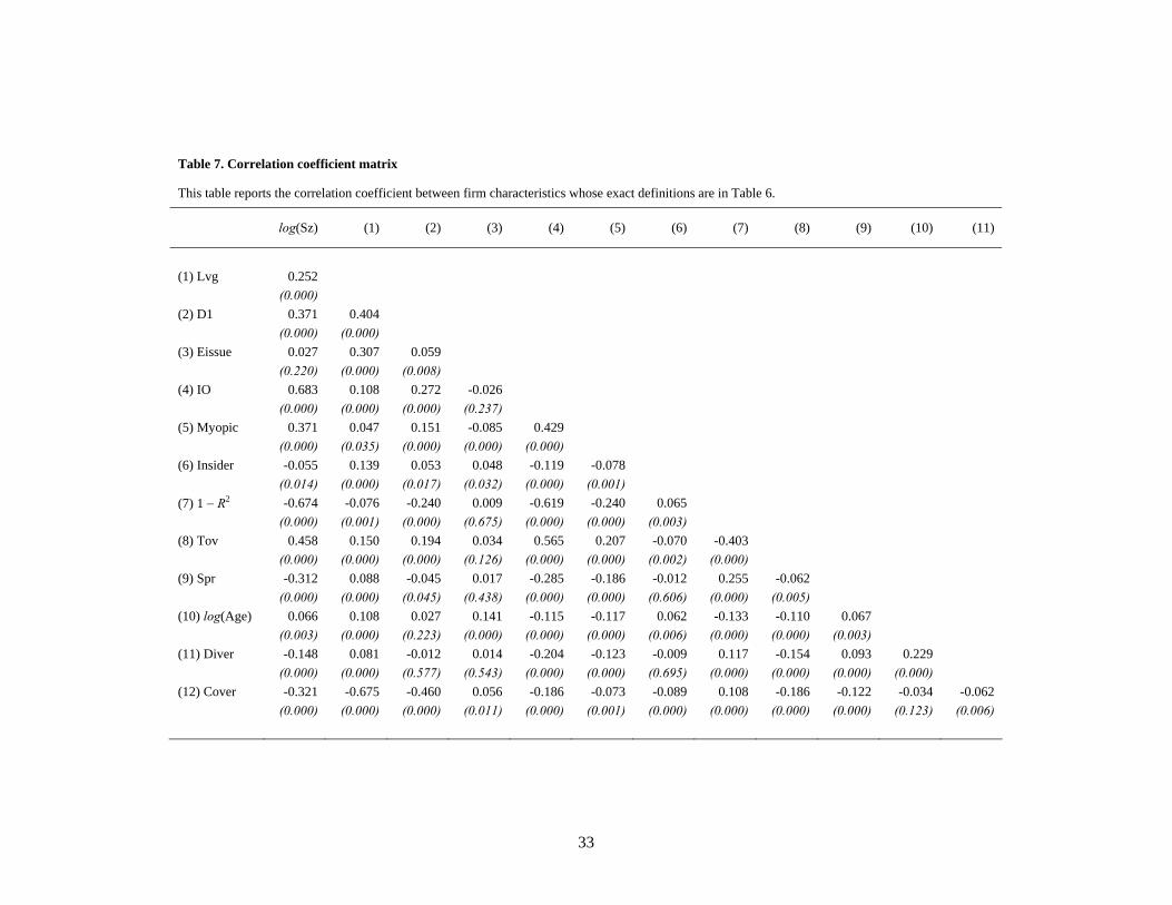
Table 7. Correlation coefficient matrix

This table reports the correlation coefficient between firm characteristics whose exact definitions are in Table 6.

log(Sz) (1) (2) (3) (4) (5) (6) (7) (8) (9) (10) (11)

(1) Lvg 0.252 (0.000) (2) D1 0.371 0.404 (0.000) (0.000) (3) Eissue 0.027 0.307 0.059 (0.220) (0.000) (0.008) (4) IO 0.683 0.108 0.272 -0.026 (0.000) (0.000) (0.000) (0.237) (5) Myopic 0.371 0.047 0.151 -0.085 0.429 (0.000) (0.035) (0.000) (0.000) (0.000) (6) Insider -0.055 0.139 0.053 0.048 -0.119 -0.078 (0.014) (0.000) (0.017) (0.032) (0.000) (0.001) (7) 1 − R2 -0.674 -0.076 -0.240 0.009 -0.619 -0.240 0.065 (0.000) (0.001) (0.000) (0.675) (0.000) (0.000) (0.003) (8) Tov 0.458 0.150 0.194 0.034 0.565 0.207 -0.070 -0.403 (0.000) (0.000) (0.000) (0.126) (0.000) (0.000) (0.002) (0.000) (9) Spr -0.312 0.088 -0.045 0.017 -0.285 -0.186 -0.012 0.255 -0.062 (0.000) (0.000) (0.045) (0.438) (0.000) (0.000) (0.606) (0.000) (0.005) (10) log(Age) 0.066 0.108 0.027 0.141 -0.115 -0.117 0.062 -0.133 -0.110 0.067 (0.003) (0.000) (0.223) (0.000) (0.000) (0.000) (0.006) (0.000) (0.000) (0.003) (11) Diver -0.148 0.081 -0.012 0.014 -0.204 -0.123 -0.009 0.117 -0.154 0.093 0.229 (0.000) (0.000) (0.577) (0.543) (0.000) (0.000) (0.695) (0.000) (0.000) (0.000) (0.000) (12) Cover -0.321 -0.675 -0.460 0.056 -0.186 -0.073 -0.089 0.108 -0.186 -0.122 -0.034 -0.062 (0.000) (0.000) (0.000) (0.011) (0.000) (0.001) (0.000) (0.000) (0.000) (0.000) (0.123) (0.006)

33

Table 8. Univariate regressions of deviation from sector equity marginal q on firm characteristics

This table reports regression results of the residuals between the 1st and 99th percentiles on firm characteristics.

(1) (2) (3) (4) (5) (6) (7) (8) (9) (10) (11) (12) (13)

Intercept 0.024 -0.003 0.022 0.009 -0.014 0.027 -0.003 -0.020 -0.020 0.001 -0.030 -0.003 -0.041 (0.203) (0.804) (0.206) (0.034) (0.045) (0.023) (0.511) (0.095) (0.017) (0.875) (0.008) (0.570) (0.000) log(Sz) -0.005 (0.116) Lvg -0.001 (0.958) D1 -0.030 (0.119) Eissue 0.912 (0.000) IO 0.027 (0.083) Myopic -0.222 (0.003) Insider -0.027 (0.658) 1 − R2 0.023 (0.156) Tov 5.771 (0.042) Spr -0.203 (0.377) log(Age) 0.014 (0.006) Diver -0.010 (0.457) Cover 0.011 (0.000) R-squares 0.1% 0.0% 0.2% 17.2% 0.1% 0.5% 0.0% 0.1% 0.3% 0.0% 0.5% 0.0% 1.8% # of obs. 1976 1970 1975 1975 1973 1976 1966 1976 1976 1976 1976 1976 1976

34

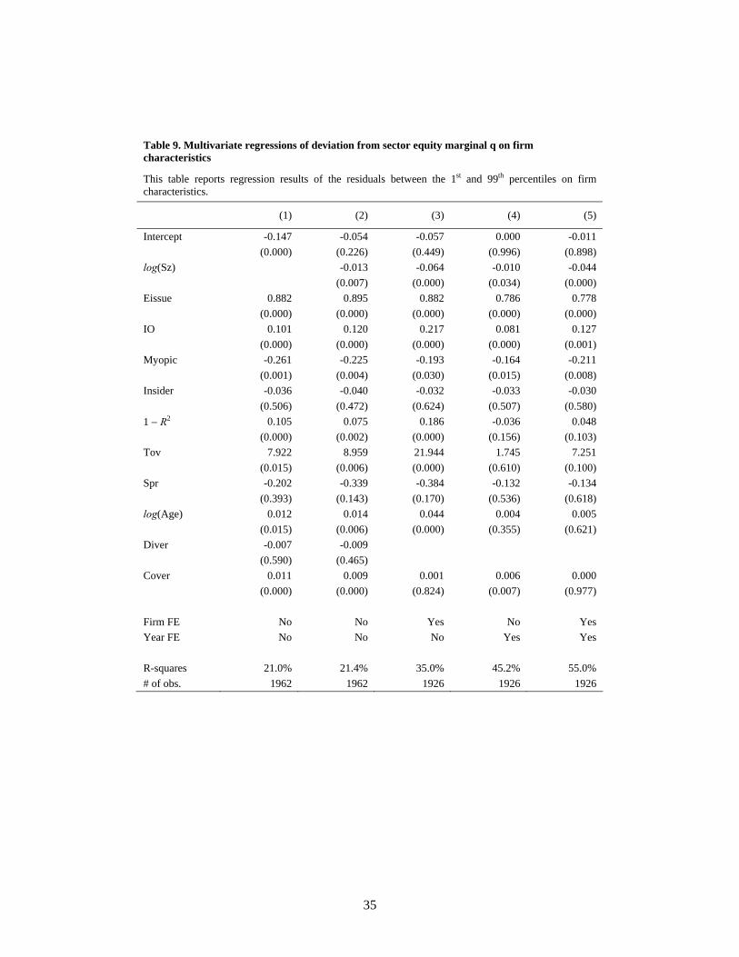
Table 9. Multivariate regressions of deviation from sector equity marginal q on firm characteristics

This table reports regression results of the residuals between the 1st and 99th percentiles on firm characteristics.

(1) (2) (3) (4) (5)

Intercept -0.147 -0.054 -0.057 0.000 -0.011 (0.000) (0.226) (0.449) (0.996) (0.898) log(Sz) -0.013 -0.064 -0.010 -0.044 (0.007) (0.000) (0.034) (0.000) Eissue 0.882 0.895 0.882 0.786 0.778 (0.000) (0.000) (0.000) (0.000) (0.000) IO 0.101 0.120 0.217 0.081 0.127 (0.000) (0.000) (0.000) (0.000) (0.001) Myopic -0.261 -0.225 -0.193 -0.164 -0.211 (0.001) (0.004) (0.030) (0.015) (0.008) Insider -0.036 -0.040 -0.032 -0.033 -0.030 (0.506) (0.472) (0.624) (0.507) (0.580) 1 − R2 0.105 0.075 0.186 -0.036 0.048 (0.000) (0.002) (0.000) (0.156) (0.103) Tov 7.922 8.959 21.944 1.745 7.251 (0.015) (0.006) (0.000) (0.610) (0.100) Spr -0.202 -0.339 -0.384 -0.132 -0.134 (0.393) (0.143) (0.170) (0.536) (0.618) log(Age) 0.012 0.014 0.044 0.004 0.005 (0.015) (0.006) (0.000) (0.355) (0.621) Diver -0.007 -0.009 (0.590) (0.465) Cover 0.011 0.009 0.001 0.006 0.000 (0.000) (0.000) (0.824) (0.007) (0.977) Firm FE No No Yes No Yes Year FE No No No Yes Yes R-squares 21.0% 21.4% 35.0% 45.2% 55.0% # of obs. 1962 1962 1926 1926 1926

35