Reinforcement Learning

Yishay Mansour

Tel-Aviv University

2

Outline

• Goal of Reinforcement Learning

• Mathematical Model (MDP)

• Planning

3

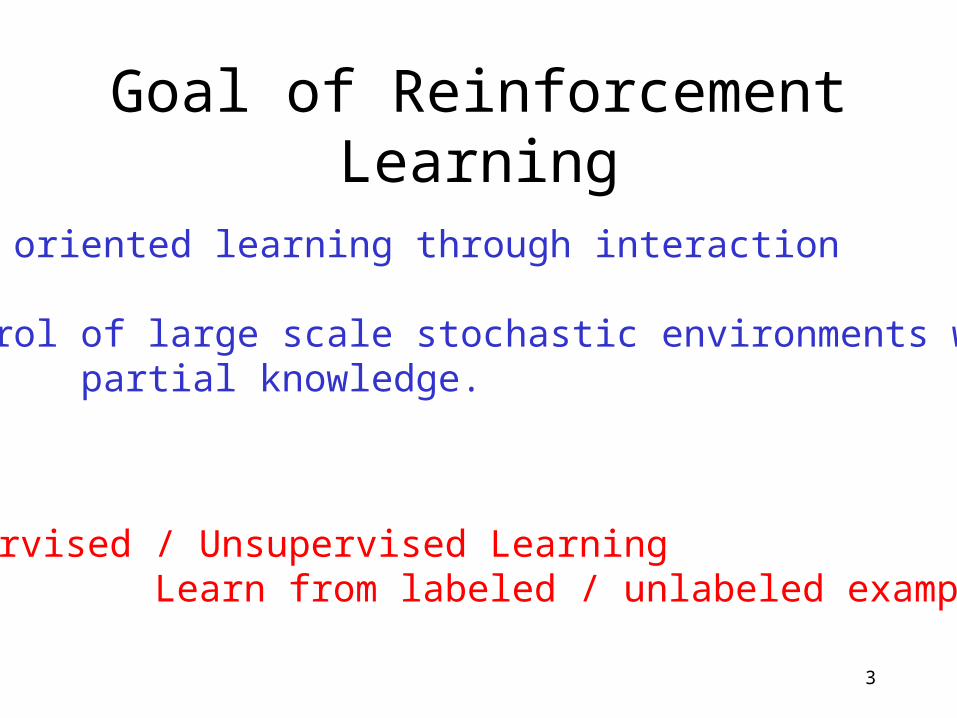
Goal of Reinforcement Learning

Goal oriented learning through interaction

Control of large scale stochastic environments with partial knowledge.

Supervised / Unsupervised Learning Learn from labeled / unlabeled examples

4

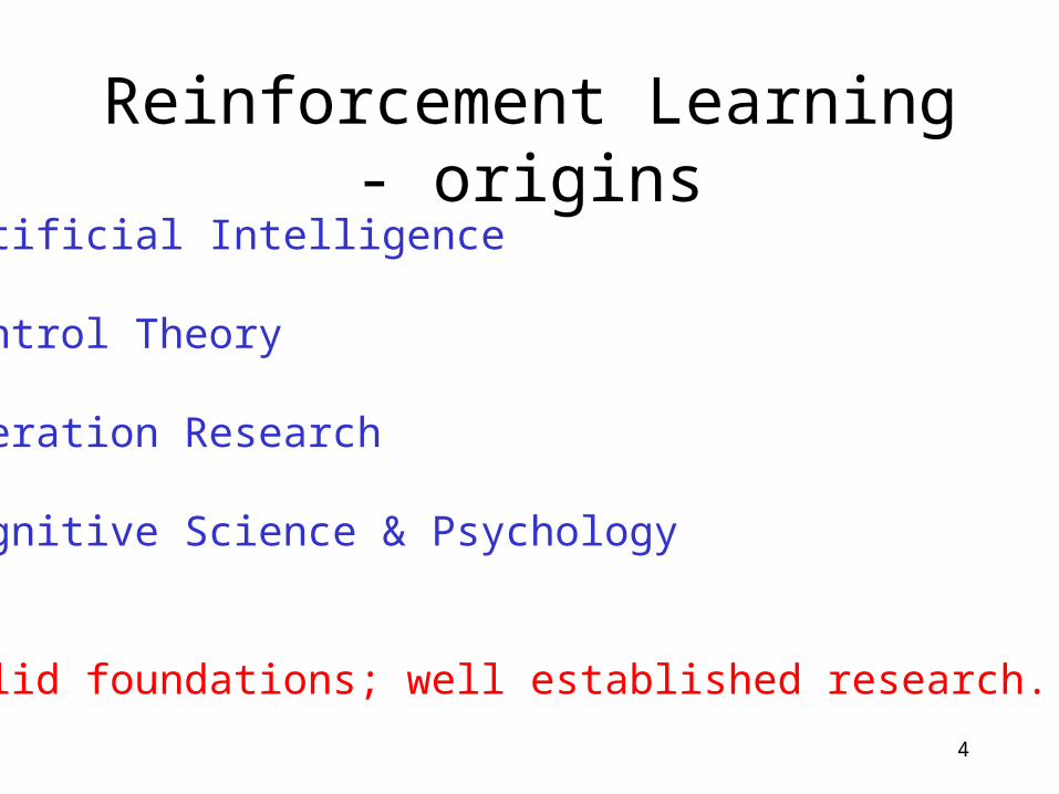
Reinforcement Learning - originsArtificial Intelligence

Control Theory

Operation Research

Cognitive Science & Psychology

Solid foundations; well established research.

5

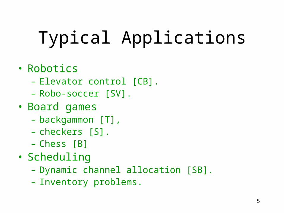
Typical Applications

• Robotics– Elevator control [CB].– Robo-soccer [SV].

• Board games– backgammon [T], – checkers [S].– Chess [B]

• Scheduling– Dynamic channel allocation [SB].– Inventory problems.

6

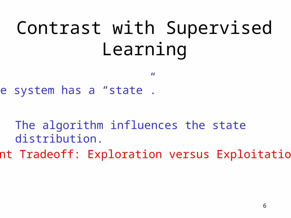
Contrast with Supervised Learning

The system has a “state”.

The algorithm influences the state distribution.

Inherent Tradeoff: Exploration versus Exploitation.

7

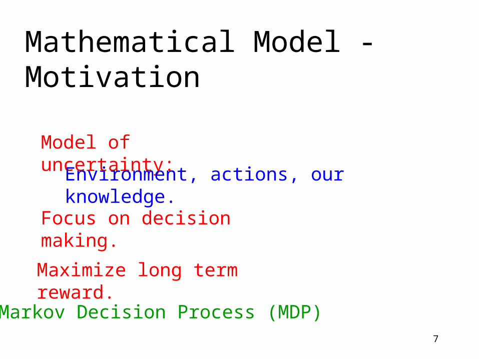
Mathematical Model - Motivation

Model of uncertainty:

Environment, actions, our knowledge.

Focus on decision making.

Maximize long term reward.

Markov Decision Process (MDP)

8

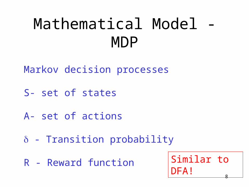
Mathematical Model - MDP

Markov decision processes

S- set of states

A- set of actions

- Transition probability

R - Reward function Similar to DFA!

9

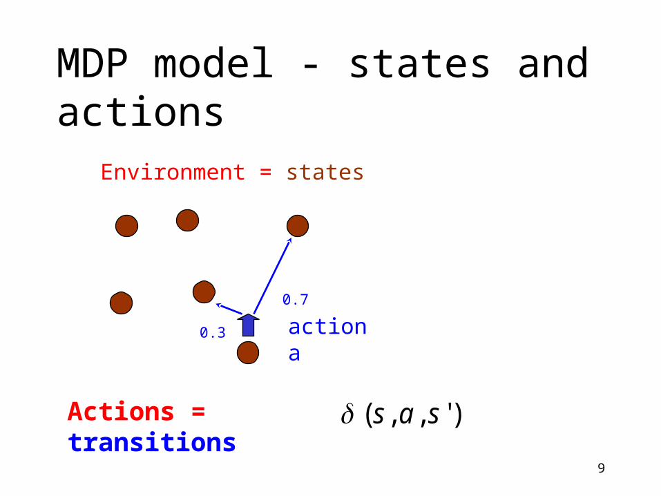
MDP model - states and actions

Actions = transitions

action a

)',,( sas

Environment = states

0.3

0.7

10

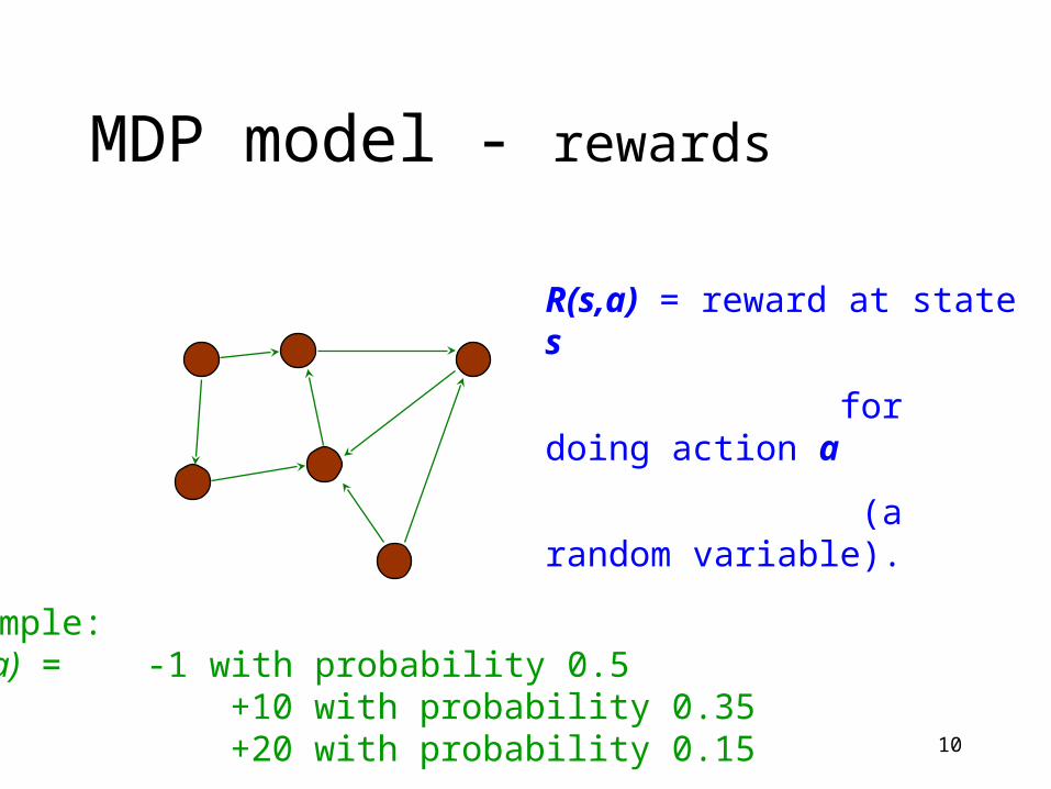
MDP model - rewards

R(s,a) = reward at state s

for doing action a

(a random variable).

Example:R(s,a) = -1 with probability 0.5 +10 with probability 0.35 +20 with probability 0.15

11

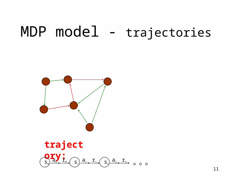
MDP model - trajectories

trajectory:

s0a0 r0 s1

a1 r1 s2a2 r2

12

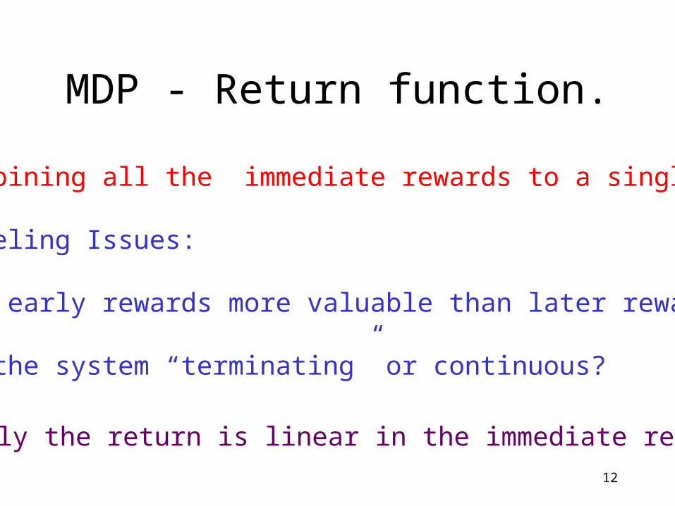
MDP - Return function.

Combining all the immediate rewards to a single value.

Modeling Issues:

Are early rewards more valuable than later rewards?

Is the system “terminating” or continuous?

Usually the return is linear in the immediate rewards.

13

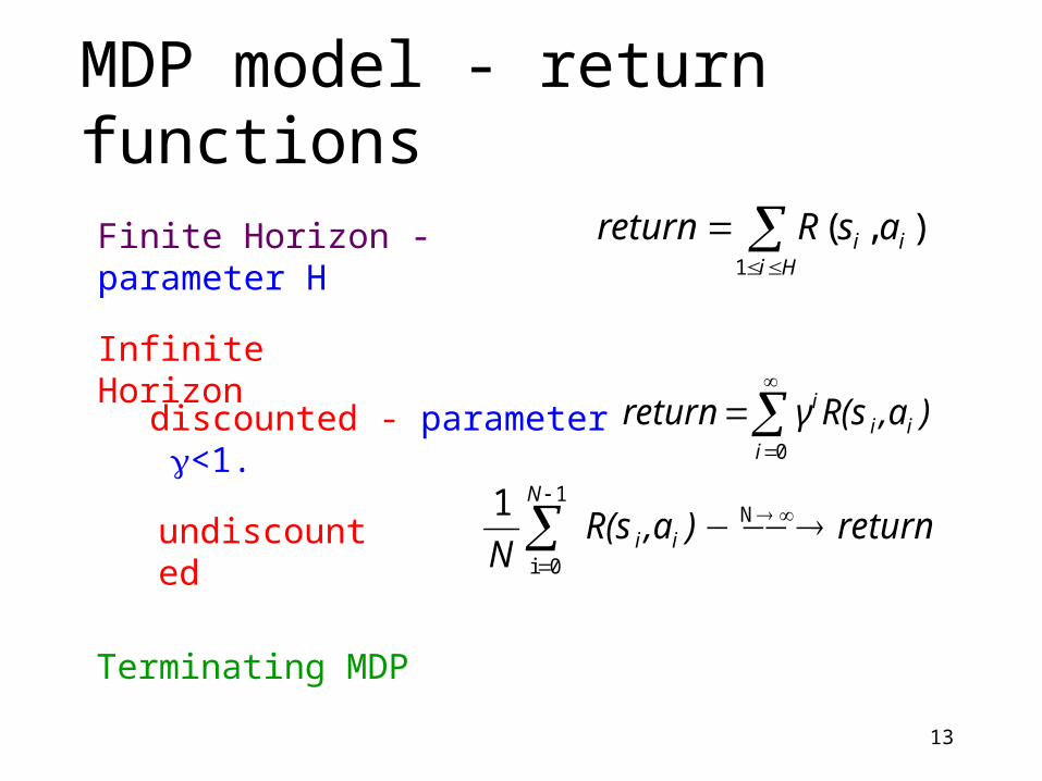
MDP model - return functions

Finite Horizon - parameter H ),(1

iHi

i asRreturn

Infinite Horizon

discounted - parameter <1. ),aR(sγreturn iii

i

0

undiscounted return),aR(sN ii

N

N

1

0i

1

Terminating MDP

14

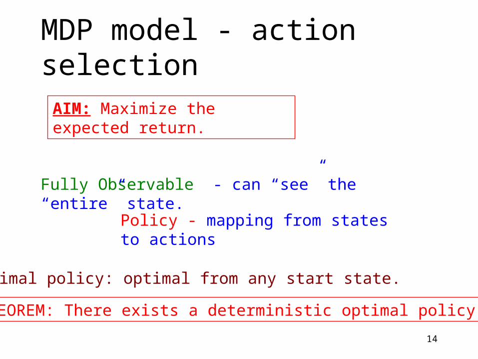
MDP model - action selection

Policy - mapping from states to actions

Fully Observable - can “see” the “entire” state.

AIM: Maximize the expected return.

Optimal policy: optimal from any start state.

THEOREM: There exists a deterministic optimal policy

15

Contrast with Supervised Learning

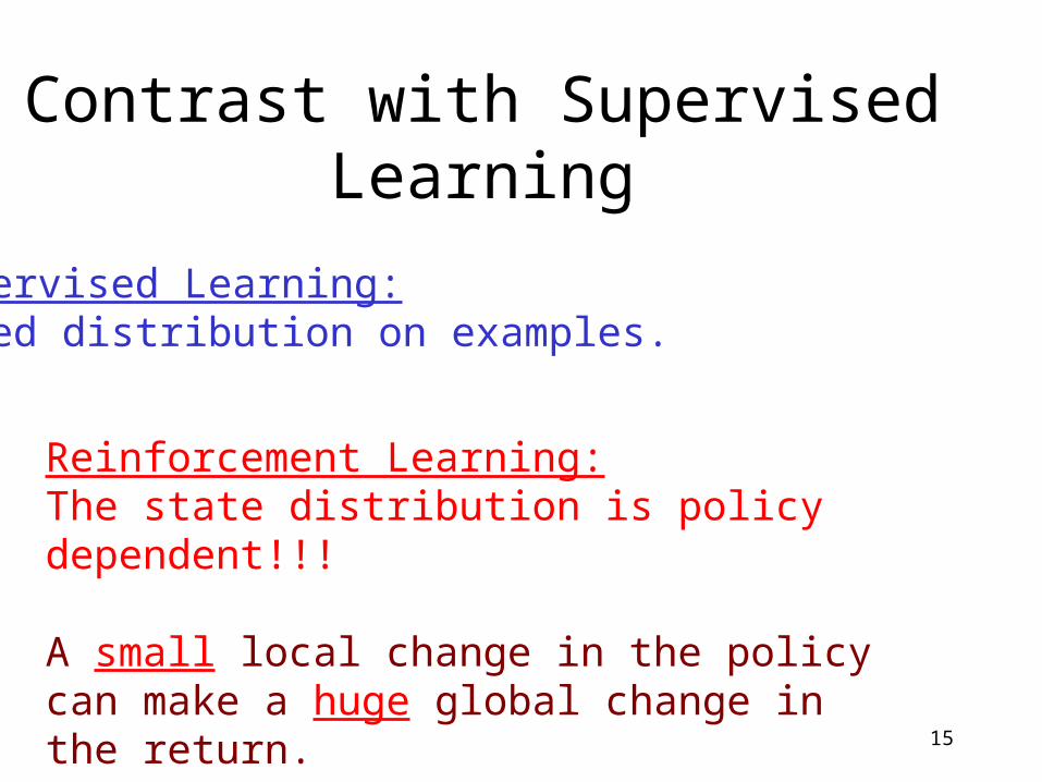
Supervised Learning:Fixed distribution on examples.

Reinforcement Learning:The state distribution is policy dependent!!!

A small local change in the policy can make a huge global change in the return.

16

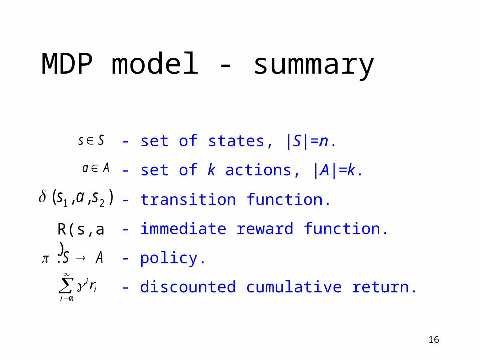
MDP model - summary

- set of states, |S|=n.

- set of k actions, |A|=k.

- transition function.

- immediate reward function.

- policy.

- discounted cumulative return.

),,( 21 sas

Ss

Aa

R(s,a)

AS :

ii

ir

0

17

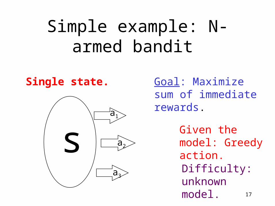
Simple example: N- armed bandit

Single state.

a1

a2

a3

s

Goal: Maximize sum of immediate rewards.

Difficulty: unknown model.

Given the model: Greedy action.

18

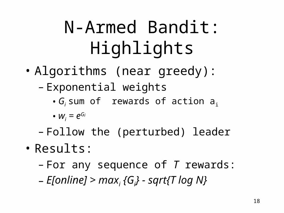
N-Armed Bandit: Highlights

• Algorithms (near greedy):– Exponential weights

• Gi sum of rewards of action ai

• wi = eGi

– Follow the (perturbed) leader

• Results:– For any sequence of T rewards:

– E[online] > maxi {Gi} - sqrt{T log N}

19

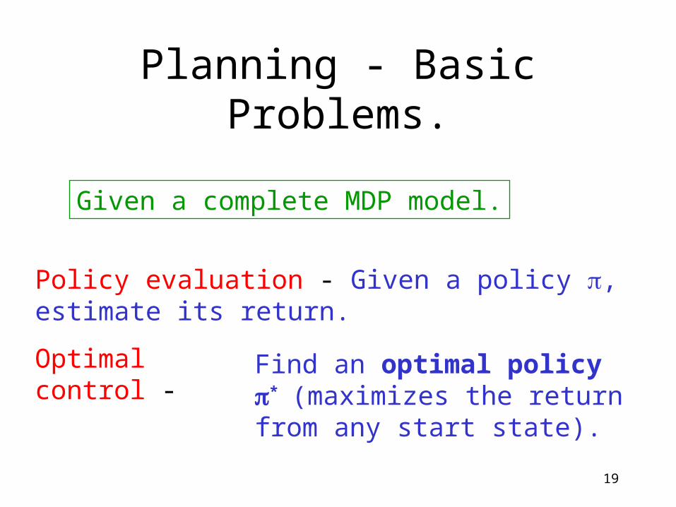
Planning - Basic Problems.

Policy evaluation - Given a policy , estimate its return.

Optimal control - Find an optimal policy *(maximizes the return from any start state).

Given a complete MDP model.

20

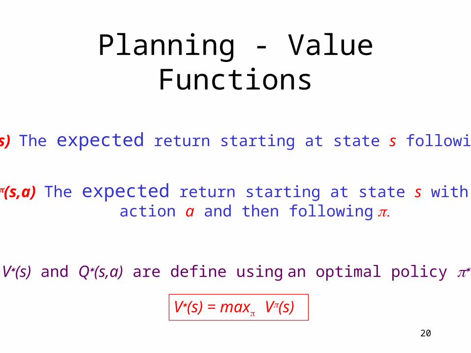
Planning - Value Functions

V(s) The expected return starting at state s following

Q(s,a) The expected return starting at state s with action a and then following

V(s) and Q(s,a) are define using an optimal policy .

V(s) = max V(s)

21

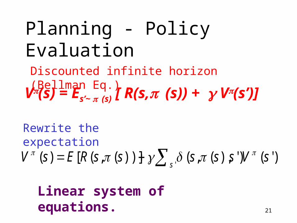
Planning - Policy Evaluation

Discounted infinite horizon (Bellman Eq.)

Rewrite the expectation

)'()'),(,())](,([)('

sVsssssREsVs

Linear system of equations.

V(s) = Es’~ (s) [ R(s,(s)) + V(s’)]

22

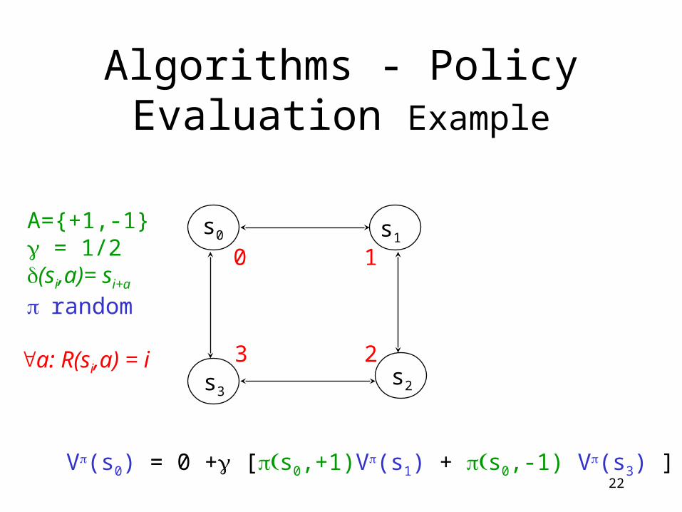
Algorithms - Policy Evaluation Example

A={+1,-1} = 1/2(si,a)= si+a

random

s0 s1

s3s2

0 1

23

V(s0) = 0 + [s0,+1)V(s1) + s0,-1) V(s3) ]

a: R(si,a) = i

23

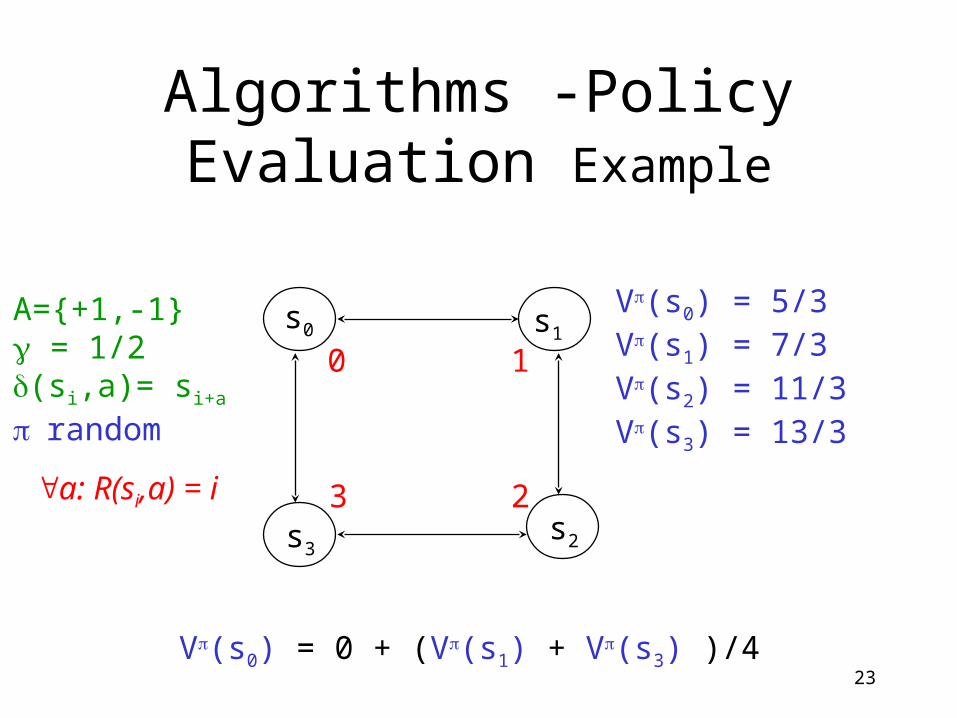
Algorithms -Policy Evaluation Example

A={+1,-1} = 1/2(si,a)= si+a

random

s0 s1

s3s2

a: R(si,a) = i

0 1

23

V(s0) = 0 + (V(s1) + V(s3) )/4

V(s0) = 5/3V(s1) = 7/3V(s2) = 11/3V(s3) = 13/3

24

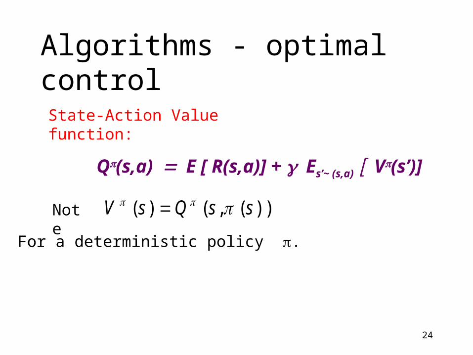
Algorithms - optimal control

State-Action Value function:

Note ))(,()( ssQsV

Q(s,a)E [ R(s,a)] + Es’~ (s,a) V(s’)]

For a deterministic policy .

25

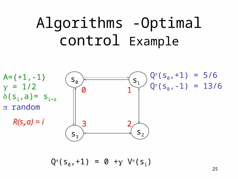
Algorithms -Optimal control Example

A={+1,-1} = 1/2(si,a)= si+a

random

s0 s1

s3s2

R(si,a) = i

0 1

23

Q(s0,+1) = 0 + V(s1)

Q(s0,+1) = 5/6Q(s0,-1) = 13/6

26

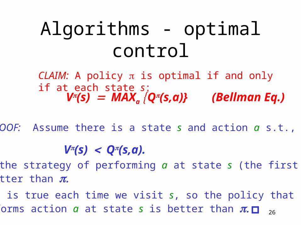
Algorithms - optimal control

CLAIM: A policy is optimal if and only if at each state s:

V(s)MAXa Q(s,a)} (Bellman Eq.)

PROOF: Assume there is a state s and action a s.t.,

V(s)Q(s,a).Then the strategy of performing a at state s (the first time)is better than This is true each time we visit s, so the policy thatperforms action a at state s is better than

27

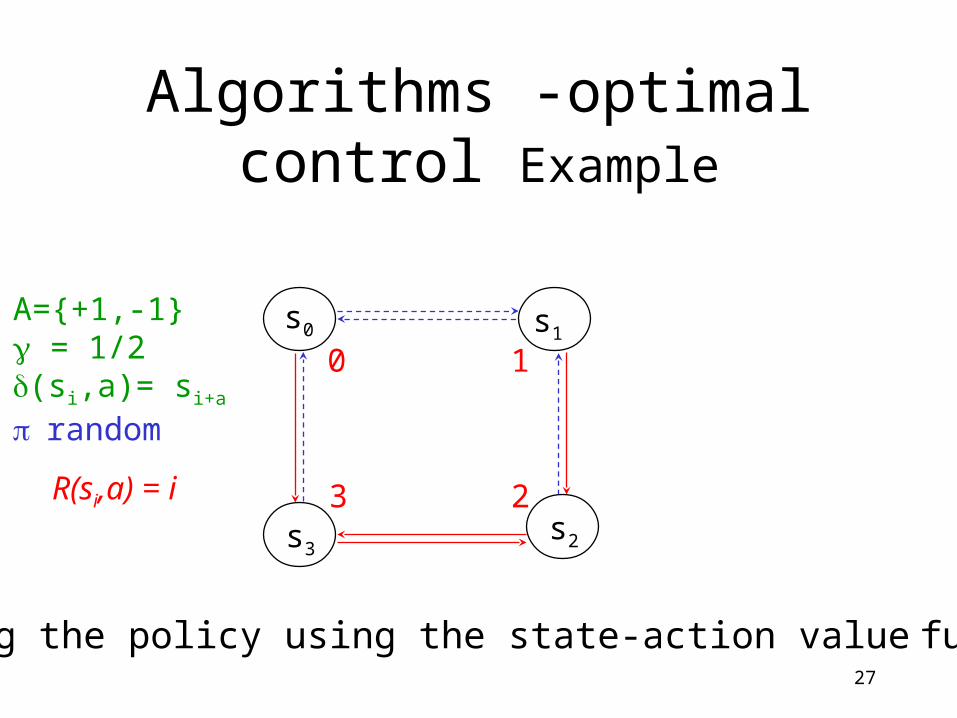
Algorithms -optimal control Example

A={+1,-1} = 1/2(si,a)= si+a

random

s0 s1

s3s2

R(si,a) = i

0 1

23

Changing the policy using the state-action value function.

28

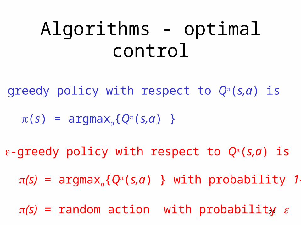
Algorithms - optimal control

The greedy policy with respect to Q(s,a) is

(s) = argmaxa{Q(s,a) }

The -greedy policy with respect to Q(s,a) is

(s) = argmaxa{Q(s,a) } with probability 1- and

(s) = random action with probability

29

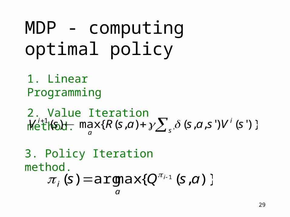
MDP - computing optimal policy

1. Linear Programming

2. Value Iteration method.

)},({maxarg)( 1 asQs i

ai

)}'( )',,(),({max)('

1 sVsasasRsVs

i

a

i

3. Policy Iteration method.

30

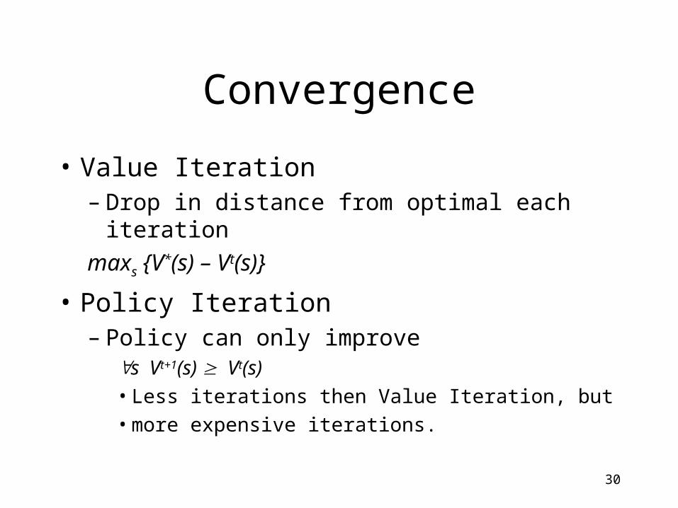
Convergence

• Value Iteration – Drop in distance from optimal each iteration

maxs {V*(s) – Vt(s)}

• Policy Iteration– Policy can only improve

s Vt+1(s) Vt(s)

• Less iterations then Value Iteration, but

• more expensive iterations.

31

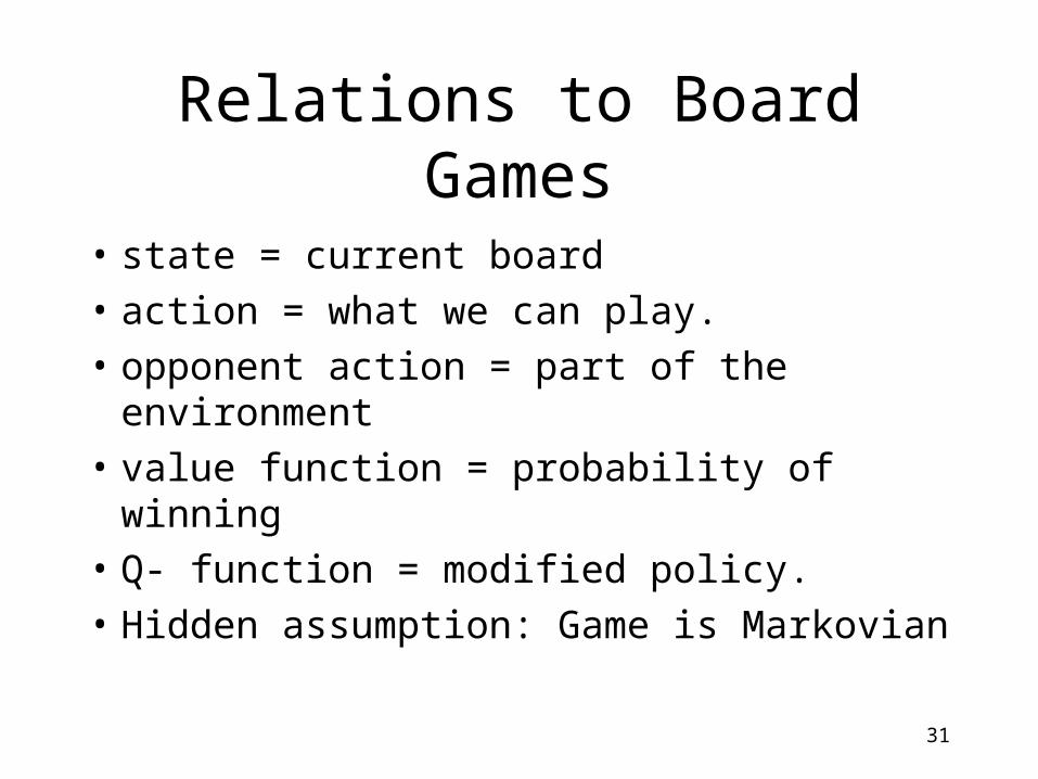
Relations to Board Games

• state = current board

• action = what we can play.

• opponent action = part of the environment

• value function = probability of winning

• Q- function = modified policy.

• Hidden assumption: Game is Markovian

32

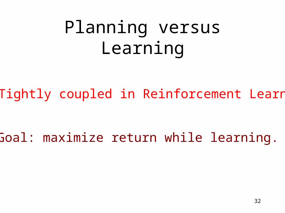
Planning versus Learning

Tightly coupled in Reinforcement Learning

Goal: maximize return while learning.

33

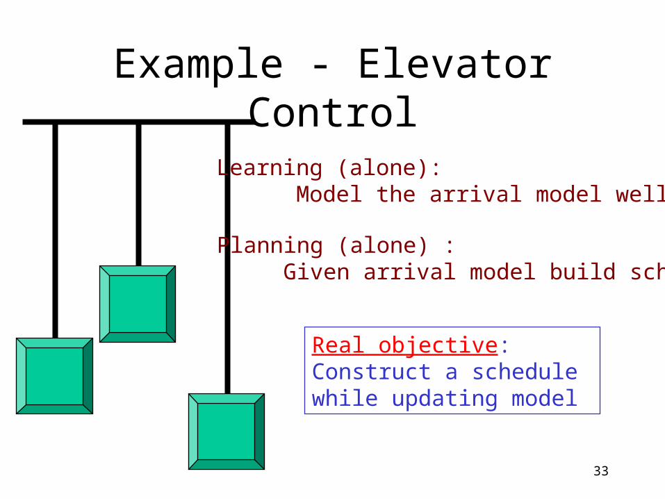
Example - Elevator Control

Planning (alone) : Given arrival model build schedule

Learning (alone): Model the arrival model well.

Real objective: Construct a schedule while updating model

34

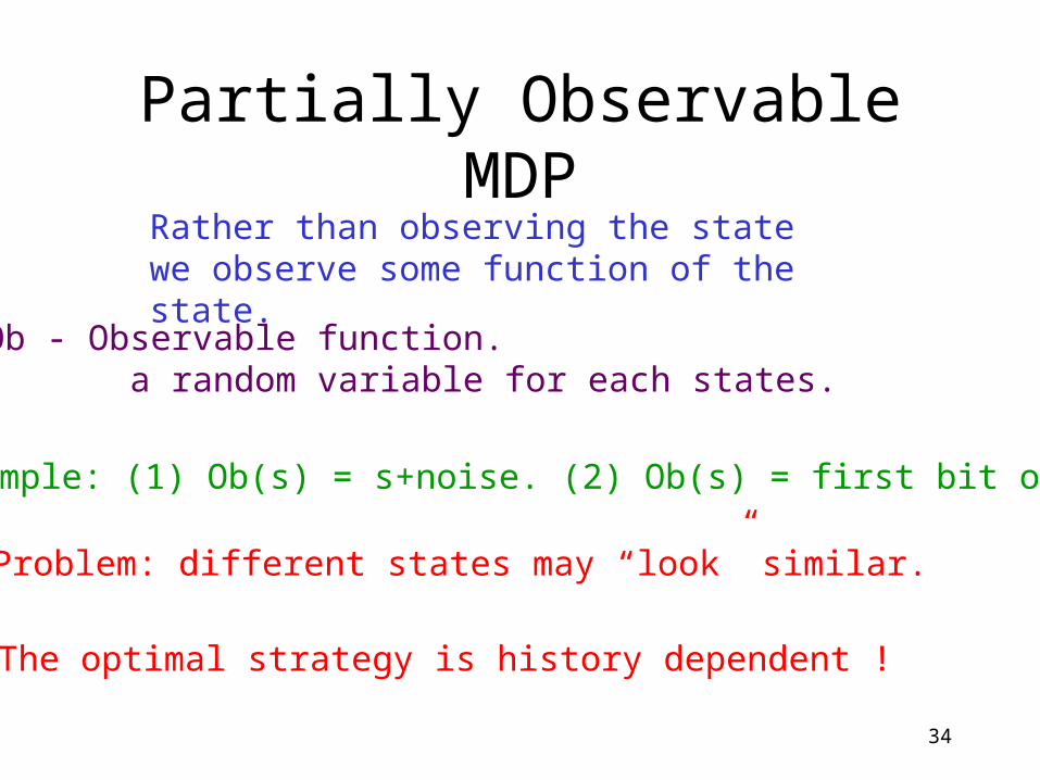
Partially Observable MDPRather than observing the state we observe some function of the state.

Ob - Observable function. a random variable for each states.

Problem: different states may “look” similar.

The optimal strategy is history dependent !

Example: (1) Ob(s) = s+noise. (2) Ob(s) = first bit of s.

35

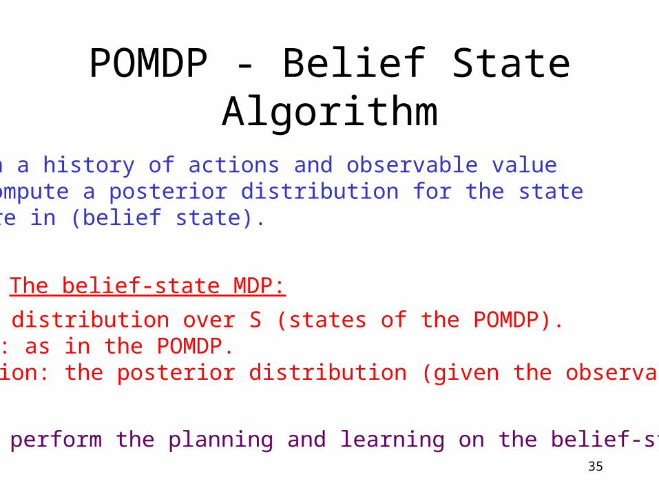
POMDP - Belief State Algorithm

Given a history of actions and observable valuewe compute a posterior distribution for the statewe are in (belief state).

The belief-state MDP:

States: distribution over S (states of the POMDP).actions: as in the POMDP.Transition: the posterior distribution (given the observation)

We can perform the planning and learning on the belief-state MDP.

36

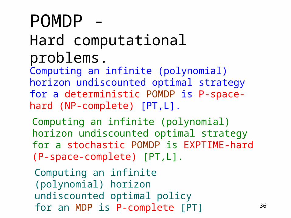
POMDP - Hard computational problems.

Computing an infinite (polynomial) horizon undiscounted optimal strategy for a deterministic POMDP is P-space-hard (NP-complete) [PT,L].

Computing an infinite (polynomial) horizon undiscounted optimal strategy for a stochastic POMDP is EXPTIME-hard (P-space-complete) [PT,L].

Computing an infinite (polynomial) horizon undiscounted optimal policy for an MDP is P-complete [PT] .

37

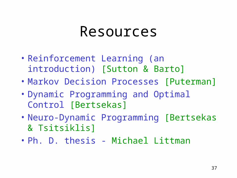
Resources

• Reinforcement Learning (an introduction) [Sutton & Barto]

• Markov Decision Processes [Puterman]

• Dynamic Programming and Optimal Control [Bertsekas]

• Neuro-Dynamic Programming [Bertsekas & Tsitsiklis]

• Ph. D. thesis - Michael Littman