Embed Size (px)
Citation preview
1
How to be a Bayesian without believing
Yoav Freund
Joint work with Rob Schapire and Yishay Mansour
2
Motivation
• Statistician: “Are you a Bayesian or a Frequentist?”
• Yoav: “I don’t know, you tell me…”• I need a better answer….
3
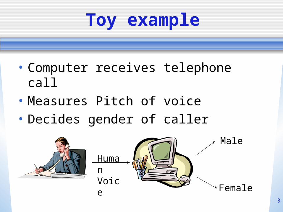
Toy example
• Computer receives telephone call• Measures Pitch of voice• Decides gender of caller
HumanVoice
Male
Female
4
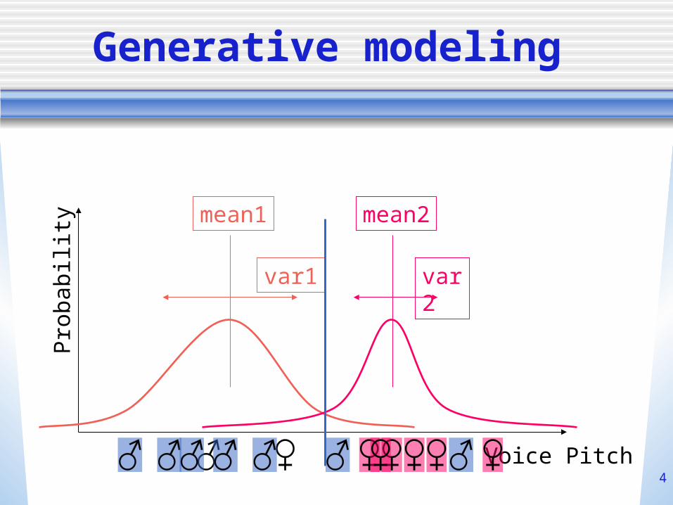
Generative modeling
Voice Pitch
Pro
babi
lity
mean1
var1
mean2
var2
5
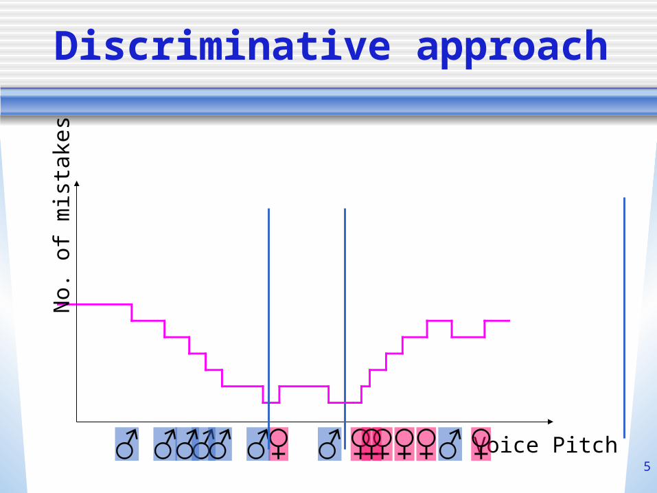
Discriminative approach
Voice Pitch
No.
of
mis
take
s
6
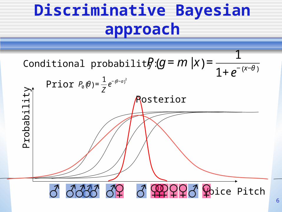
Discriminative Bayesian approach
Voice Pitch
Pro
babi
lity
Conditional probability:
€
P g = m | x( ) =1
1+ e− x−θ( )
Prior
€
P0 θ( ) =1
Ze− θ−a( )
2
Posterior
7
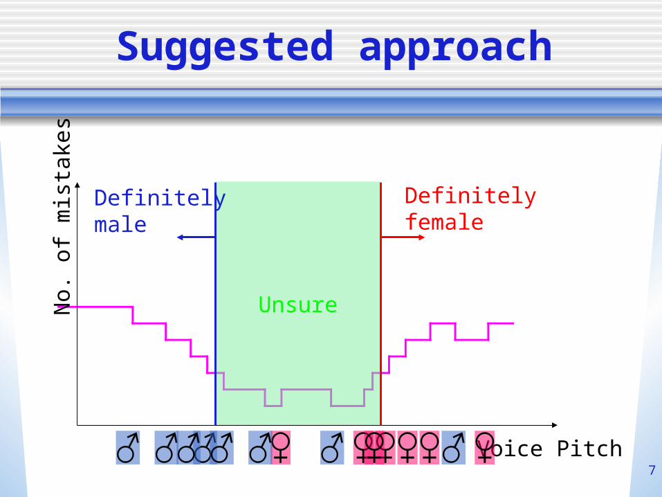
Suggested approach
Voice Pitch
No.
of
mis
take
s
Unsure
Definitelyfemale
Definitelymale
8
Formal Frameworks
For stating theorems regarding the dependence of the generalization error on the size of the training set.
9
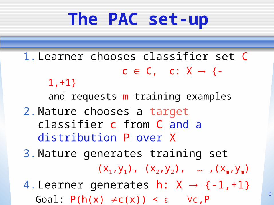
The PAC set-up
1. Learner chooses classifier set C c C, c: X {-1,+1}
and requests m training examples
2. Nature chooses a target classifier c from C and a distribution P over X
3. Nature generates training set(x1,y1), (x2,y2), … ,(xm,ym)
4. Learner generates h: X {-1,+1} Goal: P(h(x) c(x)) < c,P
10
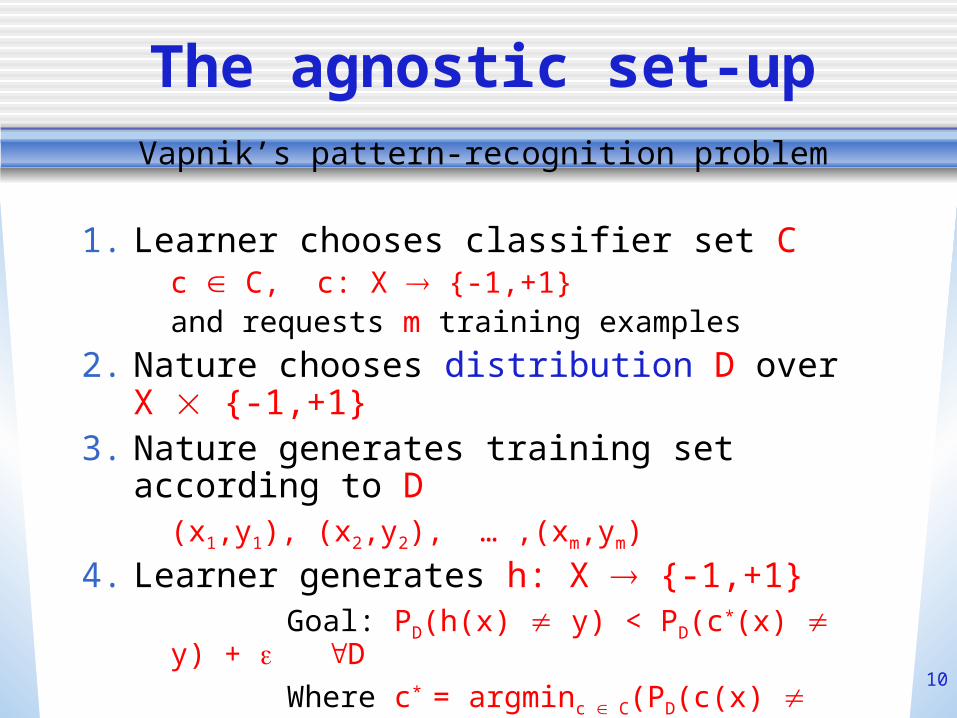
The agnostic set-up
1. Learner chooses classifier set C c C, c: X {-1,+1}
and requests m training examples
2. Nature chooses distribution D over X {-1,+1}
3. Nature generates training set according to D
(x1,y1), (x2,y2), … ,(xm,ym)
4. Learner generates h: X {-1,+1} Goal: PD(h(x) y) < PD(c*(x) y) +
D Where c* = argminc C(PD(c(x) y))
Vapnik’s pattern-recognition problem
11
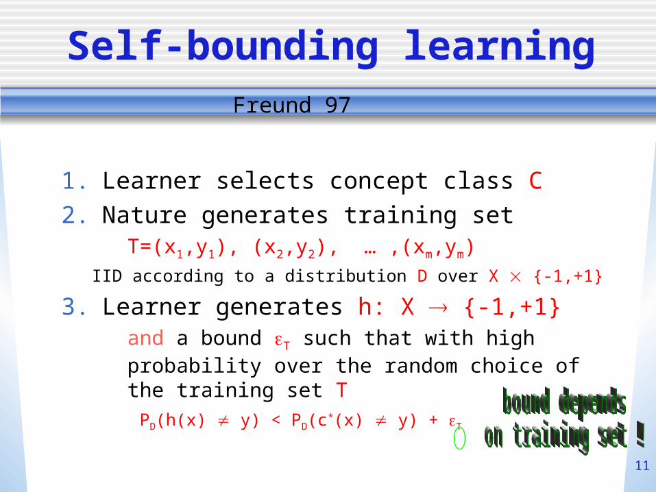
Self-bounding learning
1. Learner selects concept class C2. Nature generates training set
T=(x1,y1), (x2,y2), … ,(xm,ym)IID according to a distribution D over X {-1,+1}
3. Learner generates h: X {-1,+1} and a bound T such that with high probability over the random choice of the training set T
PD(h(x) y) < PD(c*(x) y) + T
Freund 97
12
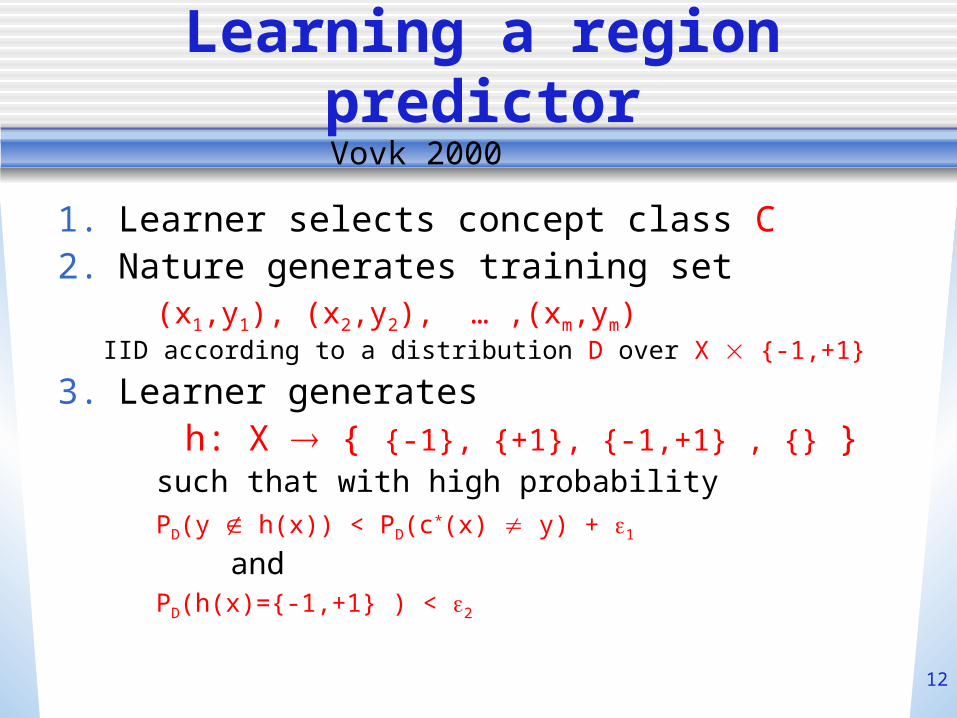
Learning a region predictor
1. Learner selects concept class C2. Nature generates training set
(x1,y1), (x2,y2), … ,(xm,ym)IID according to a distribution D over X {-1,+1}
3. Learner generates h: X { {-1}, {+1}, {-1,+1} , {} }
such that with high probability PD(y h(x)) < PD(c*(x) y) + 1
and PD(h(x)={-1,+1} ) < 2
Vovk 2000
13
Intuitions
The rough idea
14
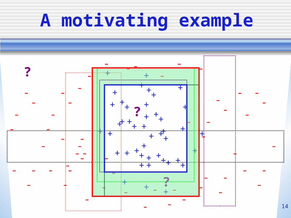
A motivating example
-
-
-+
+
+
++
+
++
++
-
-
-
-
-
-
-
-
-
--
-
-
-
-
-
--
-
-
-
-
-
-
--
-
-
-
-
-
--
-
--
-
-
-
-
-
-
+
++
+
++
+
+
++
+
++
+ +
++
+
+
+
+
+
++
+
++
+
+
++
+
++
+--
-
-- -
--
---
--
?
?
?
15
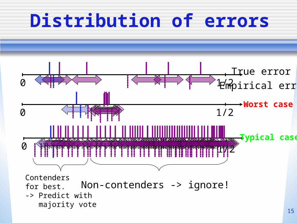
Distribution of errors
0 1/2True error
Empirical error
0 1/2Worst case
Contendersfor best.-> Predict with majority vote
Non-contenders -> ignore!
0 1/2Typical case

16
Main result
Finite concept class
17
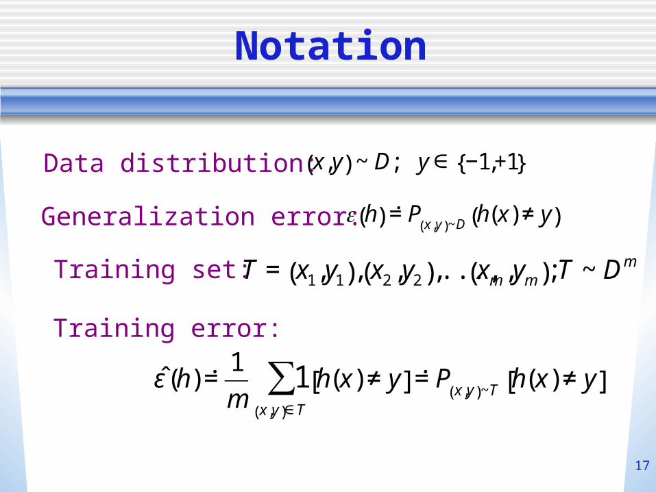
Notation
€
x,y( ) ~ D; y ∈ −1,+1{ }Data distribution:
€
h( ) ˙ = P x,y( )~D h(x) ≠ y( )Generalization error:
€
T = x1,y1( ), x2 ,y2( ),..., xm ,ym( ); T ~ DmTraining set:
€
ˆ ε (h) ˙ = 1
m1 h(x) ≠ y[ ]
x,y( )∈T
∑ ˙ = P x,y( )~T h(x) ≠ y[ ]
Training error:
18
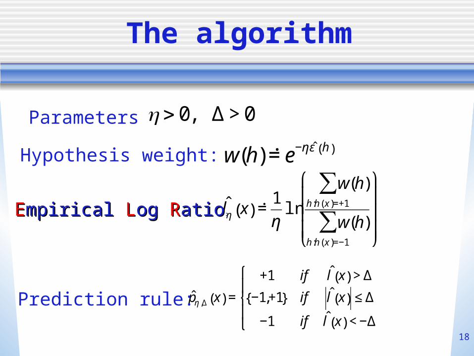
The algorithm
€
η > 0, Δ > 0Parameters
€
w(h) ˙ = e−η ˆ ε h( )Hypothesis weight:
€
ˆ l η x( ) ˙ = 1
ηln
w(h)h:h ( x)=+1
∑
w(h)h:h ( x)=−1
∑
⎛
⎝
⎜ ⎜ ⎜
⎞
⎠
⎟ ⎟ ⎟
EEmpirical mpirical LLog og RRatioatio::
€
ˆ p η ,Δ x( ) =
+1 if ˆ l x( ) > Δ
−1,+1{ } if ˆ l x( ) ≤ Δ
−1 if ˆ l x( ) < −Δ
⎧
⎨ ⎪
⎩ ⎪
Prediction rule:
19
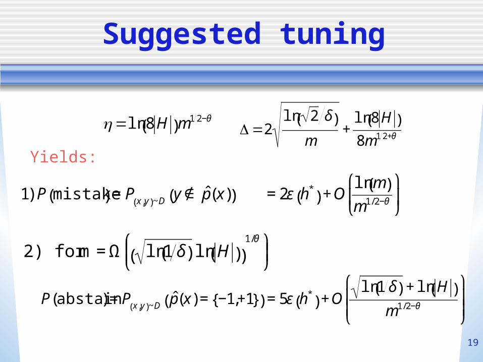
Suggested tuning
€
η=ln 8 H( )m1 2−θ
€
Δ=2ln 2 δ( )
m+
ln 8 H( )
8m1 2+θ
€
P(abstain) = P x,y( )~Dˆ p (x) = −1,+1{ }( ) = 5ε h*
( ) +Oln 1 δ( ) + ln H( )
m1/2−θ
⎛
⎝ ⎜ ⎜
⎞
⎠ ⎟ ⎟
€
2) for m = Ω ln 1 δ( ) ln H( )( )1/θ ⎛
⎝ ⎜
⎞ ⎠ ⎟
Yields:
€
1) P mistake( ) = P x,y( )~D y ∉ ˆ p (x)( ) = 2ε h*( ) +O
ln m( )m1/2−θ
⎛
⎝ ⎜
⎞
⎠ ⎟
20
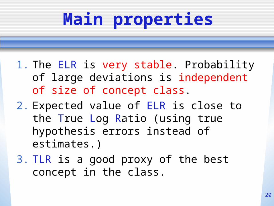
Main properties
1. The ELR is very stable. Probability of large deviations is independent of size of concept class.
2. Expected value of ELR is close to the True Log Ratio (using true hypothesis errors instead of estimates.)
3. TLR is a good proxy of the best concept in the class.
21
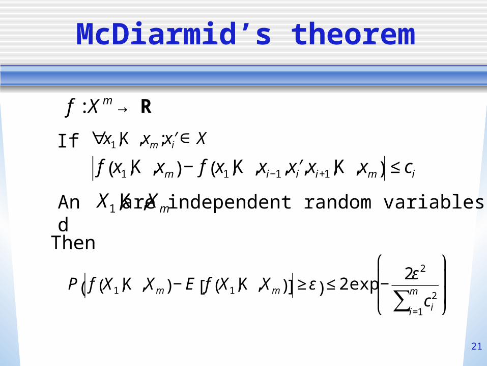
McDiarmid’s theorem
€
f : X m →R
€
∀x1,K ,xm; ′ x i ∈ X
€
f x1,K ,xm( ) − f x1,K ,xi−1, ′ x i ,xi+1,K ,xm( ) ≤ ci
If
And
€
X1,K ,Xm are independent random variables
Then
€
P f X1,K ,Xm( ) − E f X1,K ,Xm( )[ ] ≥ ε( ) ≤ 2exp −2ε 2
ci2
i=1
m
∑
⎛
⎝
⎜ ⎜
⎞
⎠
⎟ ⎟
22
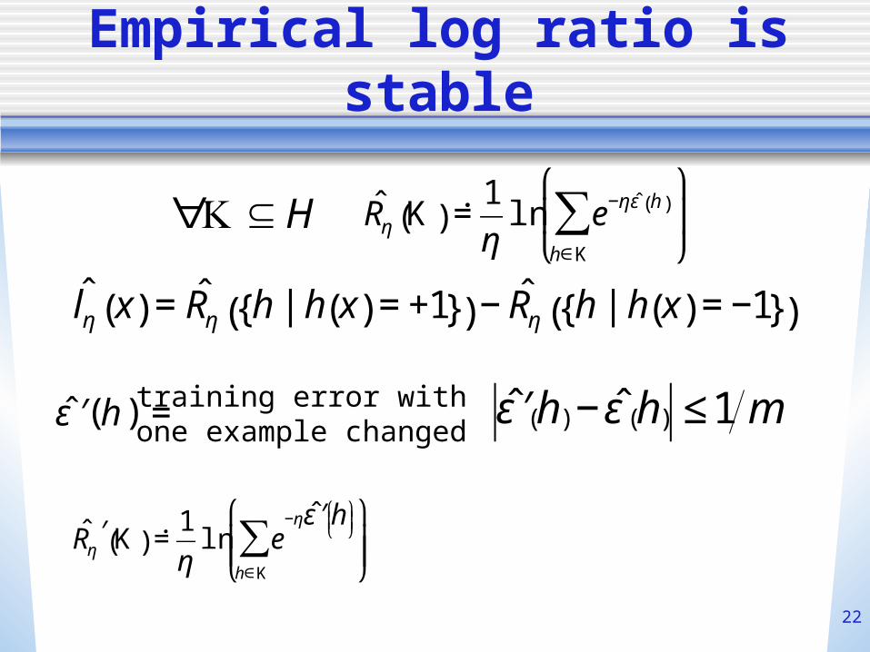
Empirical log ratio is stable
€
ˆ ′ ε h( ) = training error with one example changed
€
ˆ ′ ε h( ) − ˆ ε h( ) ≤ 1 m
€
ˆ R η′ K( ) ˙ = 1
ηln e
−η ˆ ′ ε h ⎛ ⎝ ⎜
⎞ ⎠ ⎟
h∈K
∑ ⎛
⎝ ⎜ ⎜
⎞
⎠ ⎟ ⎟
€
ˆ l η x( ) = ˆ R η h | h x( ) = +1{ }( ) − ˆ R η h | h x( ) = −1{ }( )
€
ˆ R η K( ) ˙ = 1
ηln e−η ˆ ε h( )
h∈K
∑ ⎛
⎝ ⎜
⎞
⎠ ⎟
€
∀K ⊆H
23
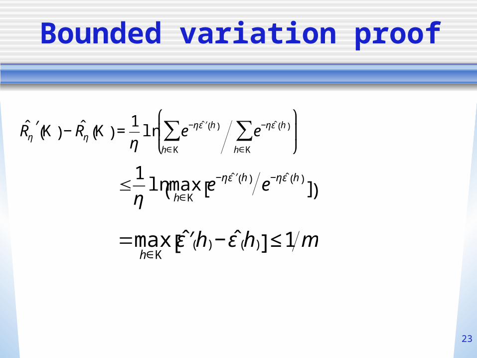
Bounded variation proof
€
ˆ R η′ K( ) − ˆ R η K( ) =1
ηln e−η ˆ ′ ε h( )
h∈K
∑ e−η ˆ ε h( )
h∈K
∑ ⎛
⎝ ⎜
⎞
⎠ ⎟
€
≤1
ηln max
h∈Ke−η ˆ ′ ε h( ) e−η ˆ ε h( )
[ ]( )
€
=maxh∈K
ˆ ′ ε h( ) − ˆ ε h( )[ ] ≤ 1 m

24
Infinite concept classes
Geometry of the concept class

25
Infinite concept classes
• Stated bounds are vacuous.• How to approximate a infinite class
with a finite class?• Unlabeled examples give useful
information.
26
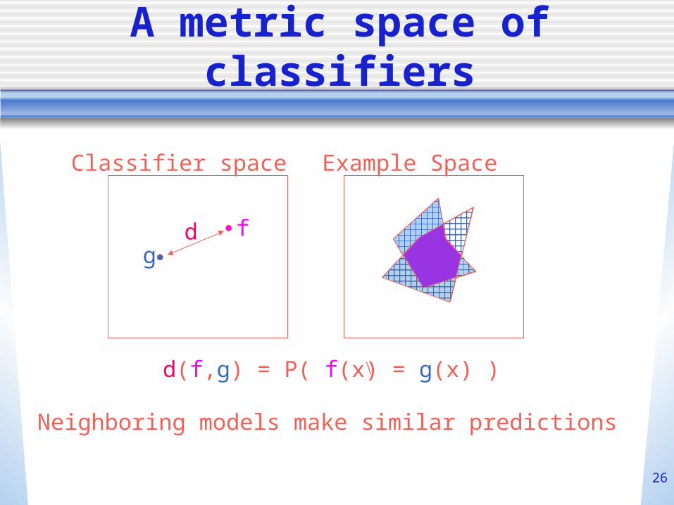
A metric space of classifiers
gf
Classifier space Example Space
d
d(f,g) = P( f(x) = g(x) )
Neighboring models make similar predictions
27
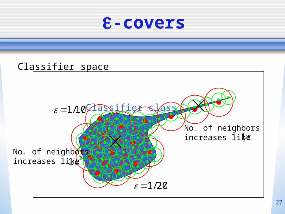
-covers
Classifier space
Classifier class
€
=1/10
€
=1/20
No. of neighborsincreases like
€
1 ε
No. of neighborsincreases like
€
1 ε 2
28
Computational issues
• How to compute the -cover?• We can use unlabeled examples to
generate cover.• Estimate prediction by ignoring
concepts with high error.
29
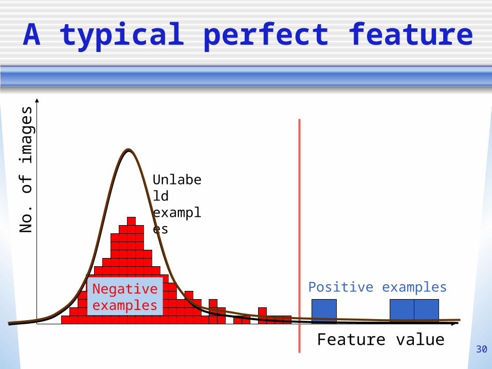
Application: comparing perfect features
• 45,000 features• Training Examples:
102 negative 2-10 positive 104 unlabeled
• >1 features have zero training error.• Which feature(s) should we use?• How to combine them?
30
A typical perfect feature
Feature value
No.
of
imag
es
Negativeexamples
Positive examples
Unlabeldexamples
31
Pseudo-Bayes for single threhold
• Set of possible thresholds is uncountably infinite
• Using an -cover over thresholds • Equivalent to using the distribution of
unlabeled examples as the prior distribution over the set of thresholds.
32
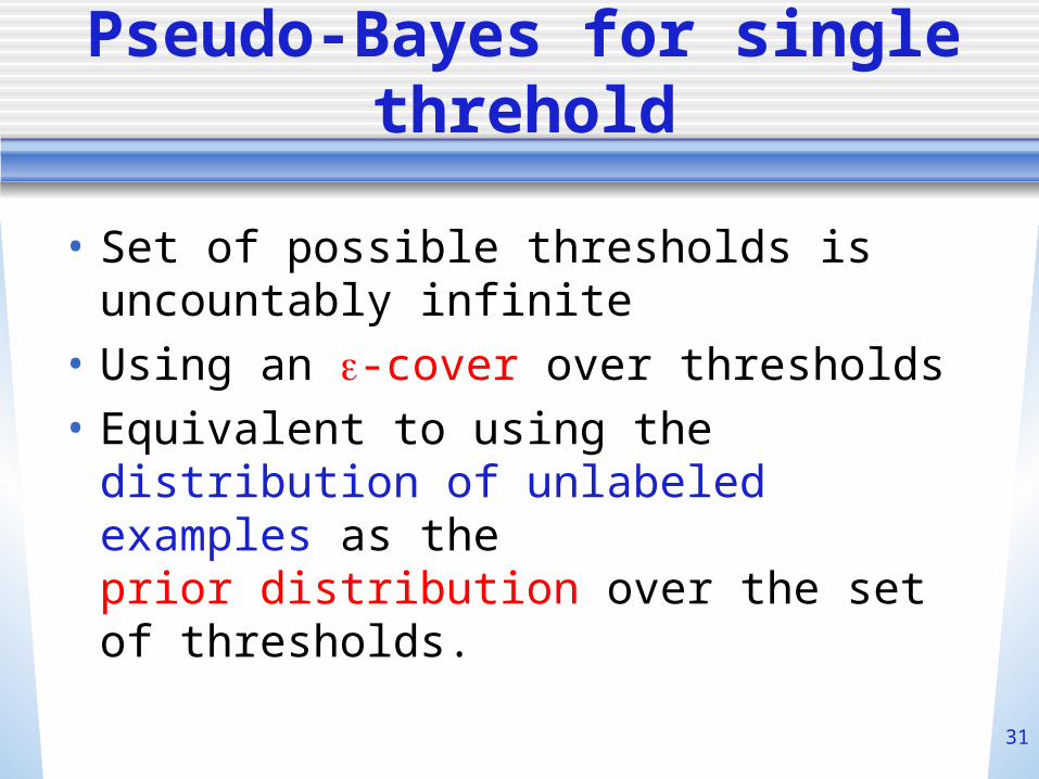
What it will do
Feature value
Negativeexamples
Prior weights Error factor
-10
+1
33
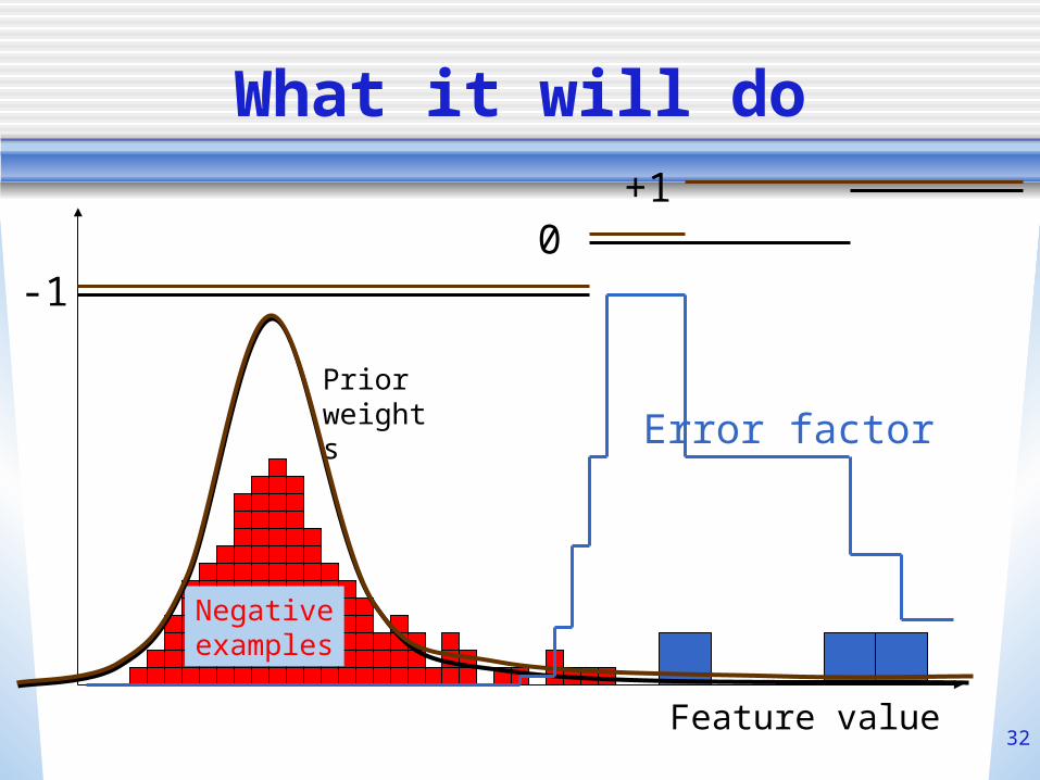
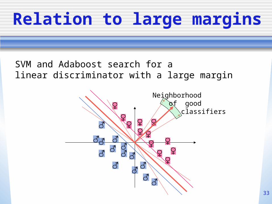
Relation to large margins
Neighborhood of good classifiers
SVM and Adaboost search for a linear discriminator with a large margin
34
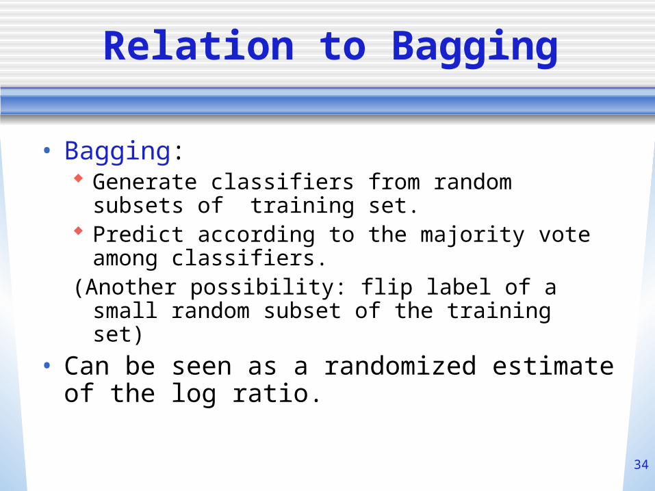
Relation to Bagging
• Bagging: Generate classifiers from random subsets of
training set. Predict according to the majority vote among
classifiers.(Another possibility: flip label of a small random
subset of the training set)
• Can be seen as a randomized estimate of the log ratio.
35
Bias/Variance for classification
• Bias: error of predicting with the sign of the True Log Ratio (infinite training set).
• Variance: additional error from predicting with the sign of the Empirical Log Ratio which is based on a finite training sample.

36
New directions
How a measure of confidence can help in practice
37
Face Detection
• Paul Viola and Mike Jones developed a face detector that can work in real time (15 frames per second).
QuickTime™ and aYUV420 codec decompressorare needed to see this picture.
38
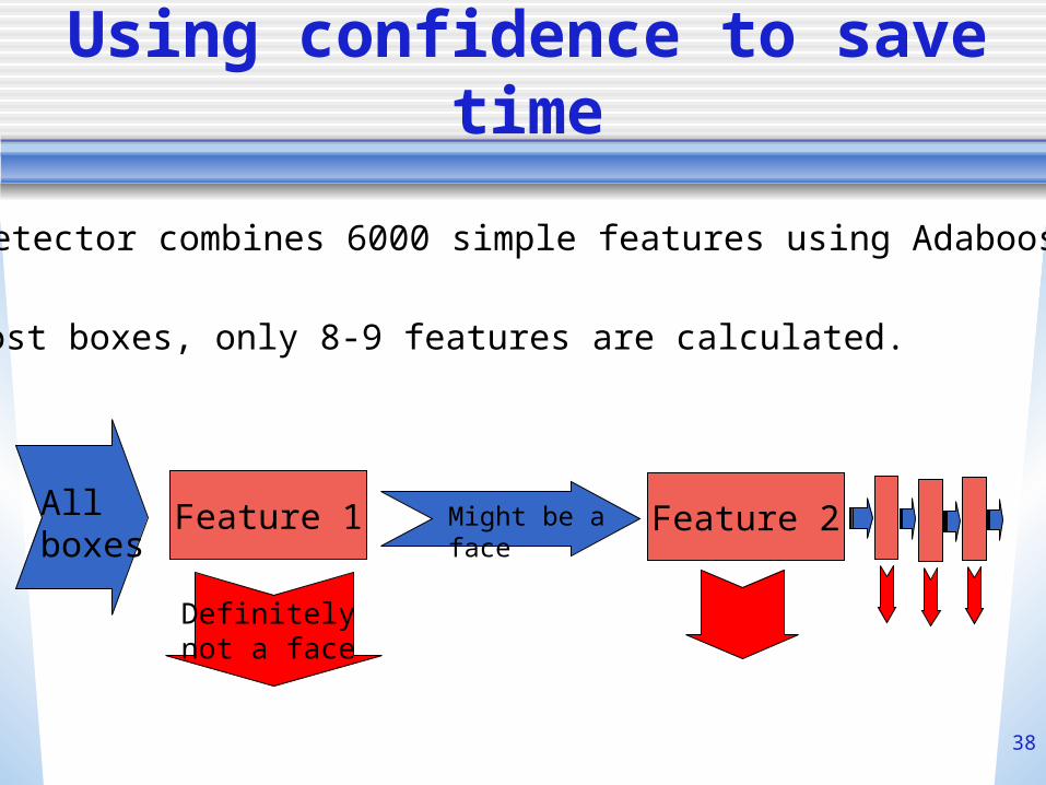
Using confidence to save time
The detector combines 6000 simple features using Adaboost.
In most boxes, only 8-9 features are calculated.
Feature 1Allboxes
Definitely not a face
Might be a face
Feature 2
39
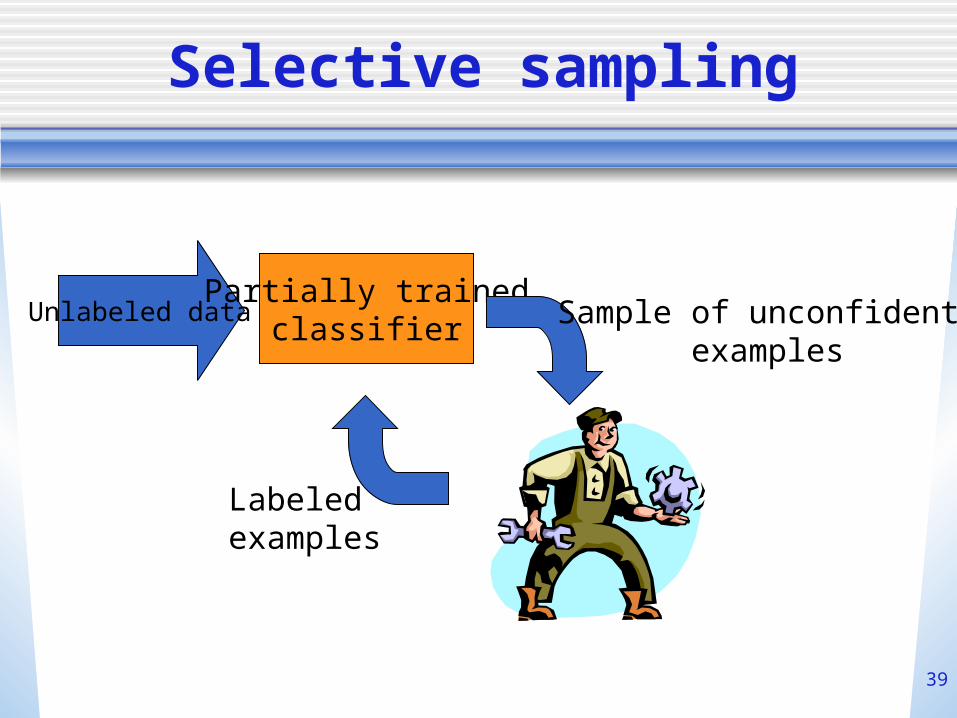
Selective sampling
Unlabeled dataPartially trained
classifier Sample of unconfident examples
Labeledexamples
40
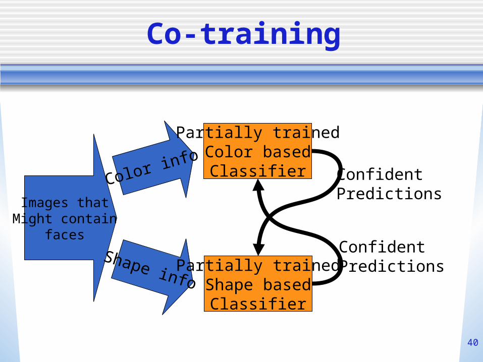
Co-training
Images thatMight contain
faces
Color info
Shape info
Partially trainedColor basedClassifier
Partially trainedShape based
Classifier
Confident Predictions
Confident Predictions
41
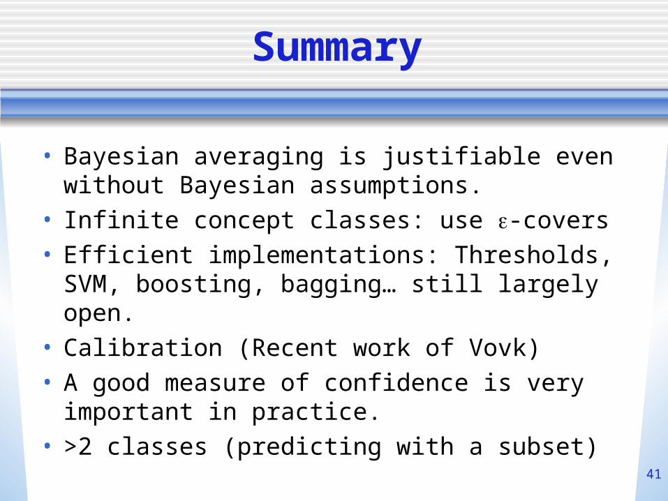
Summary
• Bayesian averaging is justifiable even without Bayesian assumptions.
• Infinite concept classes: use -covers• Efficient implementations: Thresholds, SVM,
boosting, bagging… still largely open.• Calibration (Recent work of Vovk)• A good measure of confidence is very
important in practice.• >2 classes (predicting with a subset)