Reinforcement Learning and the Power Law of

Practice: Some Analytical Results1.

Antonella Ianni2

University of Southampton (U.K.),

February, 12, 2002

1The author thanks D. Balkenborg, T. Börgers, J. Hofbauer, G. Mailath, R. Sarin,

J. Välimäki, seminar participants at the 2001 North American Winter Meetings of the

Econometric Society, at the University of Exeter and at the University of Southampton for

useful comments, and the ESRC for financial support under Research Grant R00022370.2Address for Correspondence: Department of Economics, University of Southamp-

ton, Southampton SO17 1BJ, U.K.. e-mail: a.ianni@soton.ac.uk

Abstract

Erev and Roth (1998) among others provide a comprehensive analysis of experimental

evidence on learning in games, based on a stochastic model of learning that accounts

for two main elements: the Law of Effect (positive reinforcement of actions that

perform well) and the Power Law of Practice (learning curves tend to be steeper

initially). This note complements this literature by providing an analytical study of

the properties of such learning models. Specifically, the paper shows that:

a) up to an error term, the stochastic process is driven by a system of discrete

time difference equations of the replicator type. This carries an analogy with Börgers

and Sarin (1997), where reinforcement learning accounts only for the Law of Effect.

b) if the trajectories of the system of replicator equations converge sufficiently fast,

then the probability that all realizations of the learning process over a possibly infinite

spell of time lie within a given small distance of the solution path of the replicator

dynamics becomes, from some time on, arbitrarily close to one. Fast convergence, in

the form of exponential convergence, is shown to hold for any strict Nash equilibrium

of the underlying game.

JEL: C72, C92, D83.

1 Introduction

Over the last decade there has been a growing body of research within the field of

experimental economics aimed at analyzing learning in games. Unlike field data,

experimental data allow to focus on the dynamics of the learning process of a well

specified and controlled interactive setting, where subjects are typically required to

play exactly the same game repeatedly over time, often with varying opponents.

Hence the main source of the observed dynamics is the learning process. A question

that has received increasing attention is that of how people learn to play games.

Various learning models, such as reinforcement learning (Roth and Erev (1995) and

Erev and Roth (1998) among others), belief based learning, such as various versions of

fictitious play (Fudenberg and Levine (1995) and (1998) among others) and experience

weighted attraction learning (Camerer and Ho (1999) among others) have been fitted

to the data generated by experiments. These different approaches share the common

feature that they aim at providing a learning based foundation to equilibrium theory,

by relying heavily on empirical investigation of available data.

The family of stochastic learning theories known as (positive) reinforcement seem

to perform particularly well in explaining observed behaviour in a variety of interac-

tive settings. Although specific models differ, the underlying idea of these theories

is that actions that performed well in the recent past will tend to be adopted with

higher probability by individuals who repeatedly face the same interactive environ-

ment. Specifically, the basic specification of a reinforcement learning model accounts

for two main elements: the Law of Effect (positive reinforcement learning) and the

Power Law of Practice (learning curves tend to be steeper initially). Within a grow-

ing area of research in experimental economics, Roth and Erev (1995), Erev and

Roth (1998), Sarin and Vahid (1998), Felthovich (2000), Mookherjhee and Sopher

(1997) among others provide a comprehensive analysis of experimental results that

are shown to be well explained (ex-ante and ex-post) by these models.

Despite their wide applications, very little is known on the analytical properties of

the class of reinforcement learning models. Results to date in this area include Borgers

and Sarin (1997) who study the properties of a reinforcement model that accounts

1

only for the Law of Effect; Posh (1997) who analyzes a reinforcement learning model

applied to an underlying Matching Penny game; Rustichini (1999) who characterizes

the asymptotic properties of a reinforcement model defined in a non-interactive setting

and Hopkins (2000) who investigates the asymptotic properties of a perturbed version

of a reinforcement learning model in a two-player setting.

This note contributes to this literature in that it studies the asymptotic behaviour

of reinforcement learning models, as well as the dynamics of their sample paths over

time. Specifically this paper shows that: a) up to an error term the behaviour of the

stochastic process is well described by a system of discrete time difference equation

of the replicator type (Lemma 1) and b) if the trajectories of the system of replicator

equations converge sufficiently fast, then the probability that all realization of the

learning process over a given spell of time lie within a given small distance of the

solution path of the replicator dynamics becomes arbitrarily close to one, from some

time on (Theorem 1). In particular, the paper shows that the conditions of which in b)

above are always satisfied in proximity of a strict Nash equilibrium of the underlying

game (Remark 1). Hence, if the initial condition with which the learning process

is started lies within the basin of attraction of a strict Nash equilibrium, then the

learning process converges with probability one to that Nash equilibrium.

The objective of the paper is achieved by modeling the learning process in terms of

a non-linear urn scheme that formalizes the stochastic process of individual learning.

As an example consider a situation where a finite number of players are to play

repeatedly over time a normal form game with strictly positive payoffs. Suppose

that, at each round of play, players choose actions probabilistically in the following

way: player i’s behaviour is described by an urn of infinite capacity containing balls

of as many colours, as actions available; each action is chosen with probability equal

to the proportion of balls of the corresponding coulour in the urn. Furthermore,

suppose that the proportions of balls in the urns are updated through time to reflect

the payoff obtained by players in the interaction. If player i has sampled a colour j-

ball at time t, played action j at time t and received a positive payoff, then she would

add a number of colour j-balls, exactly equal to the payoff that she got, to her urn.

As a result, at time t + 1, the proportions of balls in her urn will be different from

2

what they were at time t. In particular, the proportion of colour j (vs. colour k 6= j)balls will be higher (vs. lower) than it was, since action j has been played and has

produced a positive payoff (vs. action k has not been played and has not produced

any payoff). This formalizes a positive reinforcement effect of actions that are played,

commonly referred to as the Law of Effect. Moreover, the increase in the proportion

of colour j-balls will be decreasing in the total number of balls in the urn, meaning

that an action taken at an early stage of the learning process will have a stronger

effect on the proportion than the same action taken at a later stage. This formalizes

the fact that learning curves are steeper initially, a property usually labelled as the

Law of Practice.

Despite its simple formulation, this model generates quite a complex dynamics,

the study of which is the object of this paper. Understanding the analytical properties

of this widely used learning model is also essential as it allows to address some of the

issues noted below.

A first question that arises is whether in this model players’ behaviour becomes

stationary over time: in other words will the proportions of balls in the urn that

defines choice behaviour on the part of players converge to a limit? Posh (1997)

shows that the answer to this question is ’not necessarily so’. He studies a two player

reinforcement learning model where players repeatedly play aMatching Pennies game.

His model is analogous to the one sketched above, except that, at each time t, the

total number of balls in each urn is renormalized to t. The paper shows that, with

positive probability, this learning process cycles around the orbits of the corresponding

deterministic replicator equation. It is interesting to notice that the Law of Practice

plays a key role here. To see this, consider the same model but where, at each

time t, the total number of balls in each urn is renormalized to a constant K (other

things being left equal). Hence, the relative effect of the choice of an action on choice

probabilities is constant over time (or in other word there is no Law of Practice at

work). This different renormalization makes the model analogous to the one studied

in Börgers and Sarin (1997). Although analogous in motivation, this model produces

different results: by taking a continuous time limit, the authors show that for any

underlying game being played players will, eventually and with probability one, play

3

a pure strategy. Hence, for an underlying Matching Penny game, limit behaviour

converges1.

A second question is whether the behavioural specification of reinforcement learn-

ing model leads to optimal choices. For example, suppose there is a ’best’ action that,

when chosen, delivers the highest possible payoff. Will players who repeatedly face

this environment eventually learn to choose it? Rustichini (1998) studies the optimal

properties of a single agent reinforcement learning model that accounts for the Law of

Effect, as well as for the Law of Practice. He shows that in a linear adjustment model

like the one we consider, the process governing the proportions of balls in the urns

converges almost surely to the action that maximizes the expected payoff (where the

expectation is taken over the states of the world), whenever such an action is unique2.

This optimality property does not necessarily carry over to an interactive setting. In

fact, a key assumption in Rustichini’s paper is that ’nature’, when generating ran-

dom states of the world, does so according to an ergodic (invariant) process; this is in

general not the case in an interactive setting, where players’ behaviour may display

phenomena of lock in and path-dependence in choices. Consistently with this intu-

ition, the already mentioned Börgers and Sarin (1997) reinforcement learning model

can, with positive probability, be locked into any suboptimal state at the boundary

of the simplex. However, by explicitly modeling the Power Law of Practice, results

can be substantially strengthened to recover optimality properties of the learning al-

gorithm. Namely, a direct implication of the results we obtain in this paper is that, if

the underlying game admits a Nash equilibrium in strictly dominant strategies, then

starting from any (interior) initial condition and from some time on, any realization

of the learning process will remain arbitrarily close to that Nash equilibrium.

A third point that is worth noticing relates to underlying games that admit mul-

tiple Nash equilibria. Issues of multiplicity are endemic in many interactive settings,

a leading example being the class of coordination games. Within the literature on

learning and evolution, traditional approaches to equilibrium selection often rely on

modeled ergodicity properties of the underlying dynamic process (as for example in

Kandori, Mailath and Rob (1993) and Young (1993)). A reinforcement learning model

is, by its mere definition, non-ergodic: players’ behaviour is path-dependent and as

4

such can be absorbed in different steady configurations of play, depending on the

initial condition with which the learning process is started. A first step in handling

issues of multiplicity in a path-dependent setting relies on the full characterization

of the basins of attraction of different absorbing states (or, more generally, ergodic

sets). For a reinforcement learning model that incorporates only the Law of Effect

this connection cannot be easily established: Börgers and Sarin (1997) Remark 3

observes that, starting from any interior initial condition, the process can reach any

of its absorbing states with positive probability. On the contrary, this paper shows

that, once the Power Law of Practice is modeled, the learning process will converge

to a strict Nash equilibrium of the underlying game whenever its initial condition lies

within its basin of attraction, in a suitably defined neighbourhood.

A point raised by the above questions is that the qualitative features of the sto-

chastic process generated by learning models based on the Law of Effect are very

sensitive to whether the model also incorporates the Law of Practice. One way to

introduce a taxonomy is to notice that under the Law of Practice, the process shows

decreasing gains, in the sense that the magnitude of state transitions is decreasing

over time, while in the absence of such an effect, the process exhibits constant gains,

meaning that the effect on the state of each action choice is constant at any point

in time. Models that formalize decreasing gains typically arise endogeneously in the

framework of fictitious play (see Fudenberg and Kreps (1993), Fudenberg and Levine

(1998), Kaniovski and Young (1995), Benaim (1999) and Benaim and Hirsch (1999b)).

Constant gains are instead prominent in evolutionary models (see Binmore (1992),

Boylan (1995), Binmore, Samuelson and Vaughan (1995), Binmore and Samuelson

(1997), Benaim and Hirsch (1999a), Corradi and Sarin (2000), Benaim and Weibull

(2000)).

In the reinforcement learning model we study in this paper gains decrease endo-

geneously, since the relative effect of payoffs from the interaction on action choices

becomes smaller as players gain more experience in the learning routine. Since pay-

offs are random, so are the updated weights given to payoffs experienced at any

given point in time. Furthermore, since different players may get different streams

of payoffs over time, each player’s learning process may display a different sequence

5

of decreasing gains. However, once such sequences are renormalized to a common

scale (which can for example be the realized sequence of gains of a given player), the

results of this paper show that any realisation of the learning process can be suitably

approximated by a replicator dynamics, whenever the solutions of the latter converge

sufficiently fast. In fact, this condition is shown to hold in a neighbourhood of any

strict Nash equilibrium. Hence, if the learning process is started in proximity of a

strict Nash equilibrium, the probability that any of its realization lie within a small

distance from the solution path of the replicator dynamics, over a possibly infinite

spell of time, becomes arbitrarily close to one, from some time on. Hence the paper

sheds some light on the asymptotics of the reinforcement learning process, as well as

on its evolution over time.

The results we obtain rely on stochastic approximation techniques (Ljung (1978),

Arthur et al. (1987), (1988)) to establish the close connection between the rein-

forcement learning process and the underlying deterministic replicator equation. By

explicitly modeling the Power Law of Practice we are able to track the magnitude

of the jumps of the stochastic process, to obtain the desired result. Since replicator

dynamics have been studied extensively in biology, as well as in economics (see for

example Hofbauer and Sigmund (1998) and Weibull (1995)), results known in that

area are then used to establish that the property we require holds for any strict Nash

equilibrium of the underlying game.

The paper is organized as follows. Section 2 describes the reinforcement learning

model we study; Section 3 states the main result of the paper, the proof of which is

contained in the Appendix; and Section 4 contains some concluding remarks.

2 The model

Consider an N -player, m-action normal form game G ≡ (i = 1, ..., N;Ai; πi), whereAi = j = 1, ...,m is player i’s action space and πi : ×iAi ≡ A → < is player i’spayoff function3. Given a strategy profile a ≡ (a1, ..., ai, ..., aN) ∈ A, we denote byπi(a) the payoff to player i when a is played. For a given player i, we conventionally

denote a generic profile of action a as (ai, a−i) where the subscript −i refers to all

6

players other than i. Hence πi(j, a−i) is the payoff to player i when (s)he chooses

action j and all other players play according to a−i.

We shall think of player i’s behaviour as being characterized by urn i, an urn of

infinite capacity containing γi balls, bij > 0 of which are of colour j ∈ 1, 2, ...,m.Clearly γi ≡Pj b

ij > 0. We denote by x

ij ≡ bij/γi the proportion of colour j balls in

urn i. Player i behaves probabilistically in the sense that we take the composition

of urn i to determine i’s action choices and postulate that xij is the probability with

which player i chooses action j.

Behaviour evolves over time in response to payoff consideration in the following

way. Let xij(n) be the probability with which player i chooses action j at step n =

0, 1, 2.... . Suppose that a(n) ≡ [j, a−i(n)] is the profile of actions played at step nand πi(j, a−i(n)) shortened to πij(n) is the corresponding payoff gained by player i

who chose action j at step n. Then exactly πij(n) balls of colour j are added to urn

i at step n. At step n+ 1 the resulting composition of urn i, will be:

xij(n+ 1) ≡ bij(n+ 1)

γi(n+ 1)=bij(n) + π

ij(n)

γi(n) + πij(n)(1)

xik(n+ 1) ≡ bik(n+ 1)

γi(n+ 1)=

bik(n)

γi(n) + πij(n)for k 6= j

If payoffs are positive (as will be assumed throughout) the above new urn compo-

sition reflects two facts: first the proportion of balls of colour j (vs. k 6= j) increases(vs. decreases) from step n to step n + 1, formalizing a positive (vs. negative) rein-

forcement for action j (vs. action k), and second, since γi appears at the denominator,

the strength of the aforementioned reinforcement is decreasing in the total number

of balls in urn i.We label the first effect as reinforcement and we refer to the second

as the law of practice.

It is instructive to rewrite (1) by recalling that bij(n) ≡ xij(n)γi(n), as:

xij(n+ 1) = xij(n)

·1− πij(n)

γi(n) + πij(n)

¸+

πij(n)

γi(n) + πij(n)(2)

xik(n+ 1) = xik(n)

·1− πij(n)

γi(n) + πij(n)

¸for k 6= j

This shows that conditional upon a(n) ≡ [ai(n) = j, a−i(n)] being played at step n,player i updates her state by taking a weighted average of her old state and a unit

7

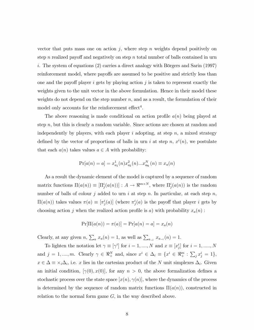
vector that puts mass one on action j, where step n weights depend positively on

step n realized payoff and negatively on step n total number of balls contained in urn

i. The system of equations (2) carries a direct analogy with Börgers and Sarin (1997)

reinforcement model, where payoffs are assumed to be positive and strictly less than

one and the payoff player i gets by playing action j is taken to represent exactly the

weights given to the unit vector in the above formulation. Hence in their model these

weights do not depend on the step number n, and as a result, the formulation of their

model only accounts for the reinforcement effect4.

The above reasoning is made conditional on action profile a(n) being played at

step n, but this is clearly a random variable. Since actions are chosen at random and

independently by players, with each player i adopting, at step n, a mixed strategy

defined by the vector of proportions of balls in urn i at step n, xi(n), we postulate

that each a(n) takes values a ∈ A with probability:

Pr[a(n) = a] = x1a1(n)x2a2

(n)...xNaN(n) ≡ xa(n)

As a result the dynamic element of the model is captured by a sequence of random

matrix functions Π(a(n)) ≡ [Πij(a(n))] : A → <m×N , where Πij(a(n)) is the randomnumber of balls of colour j added to urn i at step n. In particular, at each step n,

Π(a(n)) takes values π(a) ≡ [πij(a)] (where πij(a) is the payoff that player i gets bychoosing action j when the realized action profile is a) with probability xa(n) :

Pr[Π(a(n)) = π(a)] = Pr[a(n) = a] = xa(n)

Clearly, at any given n,P

a xa(n) = 1, as well asP

a−ixa−i

(n) = 1.

To lighten the notation let γ ≡ [γi] for i = 1, ...., N and x ≡ [xij ] for i = 1, ....., Nand j = 1, ....,m. Clearly γ ∈ <N+ and, since xi ∈ ∆i ≡ xi ∈ <m+ :

Pj x

ij = 1,

x ∈ ∆ ≡ ×i∆i, i.e. x lies in the cartesian product of the N unit simplexes ∆i. Given

an initial condition, [γ(0), x(0)], for any n > 0, the above formalization defines a

stochastic process over the state space [x(n), γ(n)], where the dynamics of the process

is determined by the sequence of random matrix functions Π(a(n)), constructed in

relation to the normal form game G, in the way described above.

8

We call such a process a stochastic urn dynamics U :

U ≡ (i = 1, .., N; [x(n), γ(n)];Π(a(n));n > 0)

for the underlying game G:

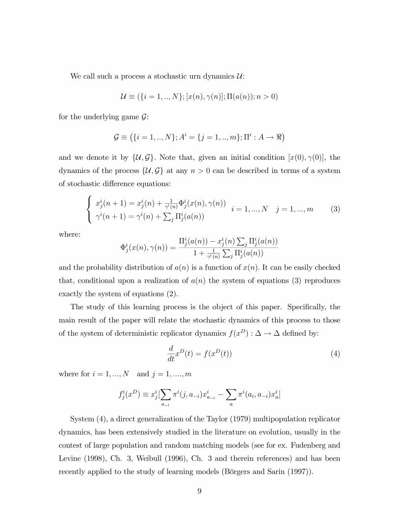
G ≡ ¡i = 1, .., N;Ai = j = 1, ..,m;Πi : A→ <¢and we denote it by U ,G. Note that, given an initial condition [x(0), γ(0)], thedynamics of the process U ,G at any n > 0 can be described in terms of a systemof stochastic difference equations: xij(n+ 1) = x

ij(n) +

1γi(n)

Φij(x(n), γ(n))

γi(n+ 1) = γi(n) +P

j Πij(a(n))

i = 1, ...,N j = 1, ...,m (3)

where:

Φij(x(n), γ(n)) =Πij(a(n))− xij(n)

Pj Π

ij(a(n))

1 + 1γi(n)

Pj Π

ij(a(n))

and the probability distribution of a(n) is a function of x(n). It can be easily checked

that, conditional upon a realization of a(n) the system of equations (3) reproduces

exactly the system of equations (2).

The study of this learning process is the object of this paper. Specifically, the

main result of the paper will relate the stochastic dynamics of this process to those

of the system of deterministic replicator dynamics f(xD) : ∆→ ∆ defined by:

d

dtxD(t) = f(xD(t)) (4)

where for i = 1, ..., N and j = 1, ....,m

f ij(xD) ≡ xij [

Xa−i

πi(j, a−i)xia−i−Xa

πi(ai, a−i)xia]

System (4), a direct generalization of the Taylor (1979) multipopulation replicator

dynamics, has been extensively studied in the literature on evolution, usually in the

contest of large population and random matching models (see for ex. Fudenberg and

Levine (1998), Ch. 3, Weibull (1996), Ch. 3 and therein references) and has been

recently applied to the study of learning models (Börgers and Sarin (1997)).

9

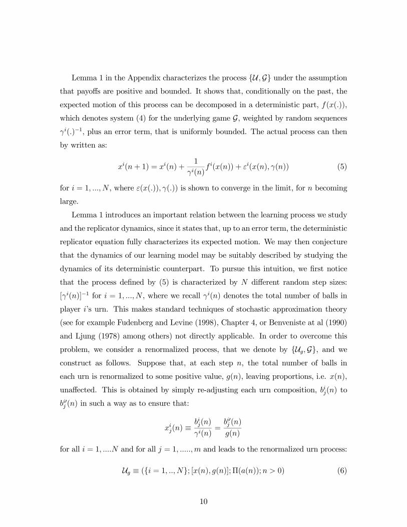
Lemma 1 in the Appendix characterizes the process U ,G under the assumptionthat payoffs are positive and bounded. It shows that, conditionally on the past, the

expected motion of this process can be decomposed in a deterministic part, f(x(.)),

which denotes system (4) for the underlying game G, weighted by random sequences

γi(.)−1, plus an error term, that is uniformly bounded. The actual process can then

by written as:

xi(n+ 1) = xi(n) +1

γi(n)f i(x(n)) + εi(x(n), γ(n)) (5)

for i = 1, ..., N , where ε(x(.)), γ(.)) is shown to converge in the limit, for n becoming

large.

Lemma 1 introduces an important relation between the learning process we study

and the replicator dynamics, since it states that, up to an error term, the deterministic

replicator equation fully characterizes its expected motion. We may then conjecture

that the dynamics of our learning model may be suitably described by studying the

dynamics of its deterministic counterpart. To pursue this intuition, we first notice

that the process defined by (5) is characterized by N different random step sizes:

[γi(n)]−1 for i = 1, ...,N , where we recall γi(n) denotes the total number of balls in

player i’s urn. This makes standard techniques of stochastic approximation theory

(see for example Fudenberg and Levine (1998), Chapter 4, or Benveniste at al (1990)

and Ljung (1978) among others) not directly applicable. In order to overcome this

problem, we consider a renormalized process, that we denote by Ug,G, and weconstruct as follows. Suppose that, at each step n, the total number of balls in

each urn is renormalized to some positive value, g(n), leaving proportions, i.e. x(n),

unaffected. This is obtained by simply re-adjusting each urn composition, bij(n) to

bi0j (n) in such a way as to ensure that:

xij(n) ≡bij(n)

γi(n)=bi0j (n)g(n)

for all i = 1, ....N and for all j = 1, .....,m and leads to the renormalized urn process:

Ug ≡ (i = 1, .., N; [x(n), g(n)];Π(a(n));n > 0) (6)

10

which dynamics is defined by: xij(n+ 1) = xij(n) +

1g(n)Φij(x(n), g(n))

g(n)i = 1, ..., N j = 1, ...,m

where Φij(., .) is as defined in (3).

By this doing, the sequence of step sizes of the renormalized process becomes

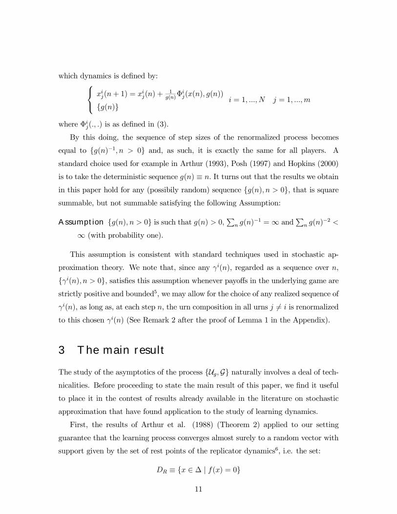
equal to g(n)−1, n > 0 and, as such, it is exactly the same for all players. Astandard choice used for example in Arthur (1993), Posh (1997) and Hopkins (2000)

is to take the deterministic sequence g(n) ≡ n. It turns out that the results we obtainin this paper hold for any (possibily random) sequence g(n), n > 0, that is squaresummable, but not summable satisfying the following Assumption:

Assumption g(n), n > 0 is such that g(n) > 0,Pn g(n)−1 =∞ and

Pn g(n)

−2 <

∞ (with probability one).

This assumption is consistent with standard techniques used in stochastic ap-

proximation theory. We note that, since any γi(n), regarded as a sequence over n,

γi(n), n > 0, satisfies this assumption whenever payoffs in the underlying game arestrictly positive and bounded5, we may allow for the choice of any realized sequence of

γi(n), as long as, at each step n, the urn composition in all urns j 6= i is renormalizedto this chosen γi(n) (See Remark 2 after the proof of Lemma 1 in the Appendix).

3 The main result

The study of the asymptotics of the process Ug,G naturally involves a deal of tech-nicalities. Before proceeding to state the main result of this paper, we find it useful

to place it in the contest of results already available in the literature on stochastic

approximation that have found application to the study of learning dynamics.

First, the results of Arthur et al. (1988) (Theorem 2) applied to our setting

guarantee that the learning process converges almost surely to a random vector with

support given by the set of rest points of the replicator dynamics6, i.e. the set:

DR ≡ x ∈ ∆ | f(x) = 0

11

whenever this consists of isolated points. As it is well known, this set typically includes

all the Nash equilibria of the underlying game G, as well as all the vertices of thesimplex ∆. Results on ‘attainability’ (i.e. convergence with positive probability to a

given rest point) within this literature (Arthur et al. (1988), Pemantle (1990)) apply

only to interior solutions, and are not of straightforward extension to the boundaries

of the simplex ∆.

Sufficient conditions that guarantee that the process does not oscillate between

different isolated rest points in DR typically require the existence of a Ljapunov func-

tion for the system (4). Theorem 1 of Ljung (1978) provides convergence conditions,

that do straightforwardly apply to our setting whenever a Ljapunov function can be

identified. Hence, convergence of the reinforcement learning process obtains for wide

classes of underlying games (see Hofbauer and Sigmund (1988) and Weibull (1995)

among others on the study of Ljapunov convergence for some classes of games).

Theorem 2 of Ljung (1978) details conditions under which the process converges

with probability one to the subset of stable rest points, i.e. the set:

DS ≡ x ∈ ∆ | f(x) = 0 and the Jacobian Df(x) hasonly eigenvalues with strictly negative real part

This set is particularly important in the study of the properties of the reinforce-

ment learning model when applied to an interactive setting, since it consists of all,

and only those, strict Nash equilibria of the underlying game. Unfortunately, the

result of Ljung (1978) is not easily applicable to our reinforcement learning model (in

particular condition D1 of Ljung (1978) cannot be easily checked).

As described below, whenever it applies, our result relates the trajectories of

the system of replicator dynamics (4) to the asymptotic paths of the reinforcement

learning model defined by (3). By doing this, we are able to show that, provided the

process is started within the basin of attraction of an asymptotically stable rest point

(and any strict Nash equilibrium is as such), the probability with which such a rest

point is reached can be made arbitrarily close to one.

Let I = nl | l ≥ 0 be a collection of indices such that 0 < n0 < n1 < .... < nl<.... . Let x(n0), x(n1), .....x(nl), .... denote the realizations of the stochastic process

12

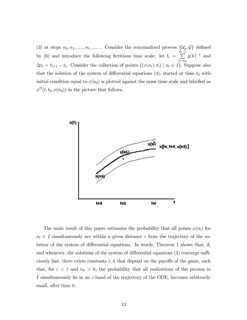
(3) at steps n0, n1, ....., nl, ..... . Consider the renormalized process Ug,G definedby (6) and introduce the following fictitious time scale: let tl =

nl−1Pk=n0

g(k)−1 and

∆tl = tl+1 − tl. Consider the collection of points (x(nl), tl) | nl ∈ I. Suppose alsothat the solution of the system of differential equations (4), started at time t0 with

initial condition equal to x(n0) is plotted against the same time scale and labelled as

xD(t, t0, x(n0)) in the picture that follows.

The main result of this paper estimates the probability that all points x(nl) for

nl ∈ I simultaneously are within a given distance ε from the trajectory of the so-

lution of the system of differential equations. In words, Theorem 1 shows that, if,

and whenever, the solutions of the system of differential equations (4) converge suffi-

ciently fast, there exists constants ε, n that depend on the payoffs of the game, such

that, for ε < ε and n0 > n, the probability that all realizations of the process in

I simultaneously lie in an ε-band of the trajectory of the ODE, becomes arbitrarily

small, after time n.

13

Theorem 1 Consider the stochastic process Ug,G (defined by system (6)). Supposepayoffs of G are bounded and strictly positive. Let the system of ODE (4) denote a

system of deterministic replicator dynamics and xD(t, t0, x) denote any time t ≥ 0

solution, when the initial condition is taken to be x at time t0. Suppose that the

following property holds over a compact set D ⊆ ∆:¯xD(t+∆t, t, x+∆x)− xD(t+∆t, t, x)¯ ≤ (1− λ∆t) |∆x| (7)

with 0 < λ < 1 and |.| denoting the Euclidean norm.Then, for all x(n0) ∈ D, there exists constants C, ε, n that depend on the game G,

such that, for ε < ε and n0 > n:

Pr

·supnl∈I

¯x(nl)− xD(tnl

, tn0 , x(n0)¯> ε

¸≤ C

ε2

NXj=n0

1

g(j)2(8)

for nl ∈ I = n0, n1, ...... N, where N = supI nl.

The above Theorem shows that the learning process stays close to the correspond-

ing trajectory of the replicator dynamics with higher probability as n0 increases, for a

given ε. The intuition behind the result is that the common gain sequence g(.)−1 of

the process Ug,G can be rescaled in such a way as to guarantee that the process x(.)stays close to xD(.) with an arbitrary high degree of precision. Notice that, since the

RHS of inequality (8) is square summable, the statement holds for any N , possibly

infinite.

Next, condition (7) is shown to hold for any strict Nash equilibrium of the under-

lying game G:

Remark 1 Let x∗ be a strict Nash equilibrium of G and denote its basin of attractionby:

B(x∗) ≡ x ∈ ∆ | limt→∞

xD(t, t0, x) = x∗

Then there exist an open set Br ≡ x ∈ ∆ | |x− x∗| < r ⊆ B(x∗) such that condition(7) stated in Theorem 1 holds in Br.

14

A straightforward implication of the above Remark is that if the stochastic process

Ug,G is started in a suitably defined neighbourhood of a strict Nash equilibrium,then the probability with which the process converges to that Nash equilibrium can

be made arbitrarily close to one.

3.1 Outline of the Proof of Theorem 1

The main result relies on a series of Lemmas.

As already mentioned, Lemma 1 shows that, whenever payoffs are positive and

bounded, the motion of the stochastic system xi(n) is driven by the deterministic

system of f i(x(n)), rescaled by a random sequence γi(n)−1, up to a convergent error

term. The key to the proof of convergence is the coupling of the error term with

the sum of a supermartingale and a quadratically integrable martingale, defined in

relation to the sigma-algebra generated by xi(k), γi(k); k = 1, ..., n. Lemma 1

applied to Ug,G allows us to re-write the process as:

xi(j(n)) = xi(n) +

j(n)−1Xs=n

1

g(s)f i(x(s)) +

j(n)−1Xs=n

εi(x(s)), g(s))

for j(n) ≥ n+1, where the last term can be made arbitrarily small by an appropriatechoice of n, since it is the difference between two converging martingales.

Lemma 2 then proceeds to show that if the process Ug,G is, at step n of itsdynamics, within a small ρ-neighbourhood of some value x, then it will remain within

a ρ-neighbourhood of x for some time after n. As such, Lemma 2 provides information

about the local behaviour of the stochastic process x(.) around x0, by characterizing

an upper bound to the spell of re-scaled time within which the process stays in a

neighbourhood of x0.

The intuition used to derive global results runs as follows. Suppose time t re-

alization of the process, x0, belongs to some interval A. Within a time interval ∆t

two factors determine the subsequent values of the process: a) the deterministic part

of the dynamics, i.e. the functions f(x(t)) started with f(x(t)) in A and b) the

noise component. If the trajectories of f(x) converge, then after this time interval,

f(x(t +∆t)) will be in some interval B ⊂ A, for all x that started in A. Hence the

15

distance between any two such trajectories will decrease over this time interval, the

more so, the longer is the time interval. According to Lemma 2, the realization of the

stochastic process will differ from the corresponding trajectories by a small quantity,

say ±C, the more so, the smaller is the time interval. Hence the stochastic processwill not diverge from its deterministic counterpart if B + 2C ≤ A. In order for thisto hold, the time interval ∆t needs to be large enough to let the trajectories of the

deterministic part converge sufficiently, but small enough to limit the noise effect.

To this aim, Lemma 3 shows that if the realization of our process x(.) lies within

ε distance from the corresponding trajectory of xD(.) at time nl, then this will also

be true at time nl+1, provided ε is small enough to guarantee that ∆tl is

a) big enough for any two trajectories of xD(.) to converge sufficiently, and

b) small enough to limit second order effects and the effects of the noise.

To conclude the proof of Theorem 1 it is then sufficient to estimate the probability

that Lemma 2 holds simultaneously for all nl.

4 Conclusions

This paper studies the analytical properties of a reinforcement learning model that

incorporates the Law of Effect (positive reinforcement of actions that perform well),

as well as the Law of Practice (the magnitude of the reinforcement effect decays

over repetitions of the game). The learning process models interaction, among a

finite set of players faced with a normal form game, that takes place repeatedly over

time. The main contribution to the literature relies on the full characterization of

the asymptotic paths of the learning process in terms of the trajectories of a system

of replicator dynamics applied to the underlying game. Regarding the asymptotics

of the process, the paper shows that if the reinforcement learning model is started in

a neighbourhood of a strict Nash equilibrium, then convergence to that equilibrium

takes place with probability arbitrarily close to one. As for the dynamics of the

process, the results show that, from some time on, any realization of the learning

process will be arbitrarily close to the trajectory of the replicator dynamics started

with the same initial condition.

16

The convergence result we obtain relies on two main facts: first by explicitly mod-

elling the Law of Practice, we are able to construct a fictituous time scale over which

any realization of the process can be studied; second, the observation that whenever

the solution of the system of replicator dynamics converge exponentially fast, the

deterministic part of the process drives the stochastic dynamics. Both requirements

are shown to be essential to establish the result.

17

Appendix

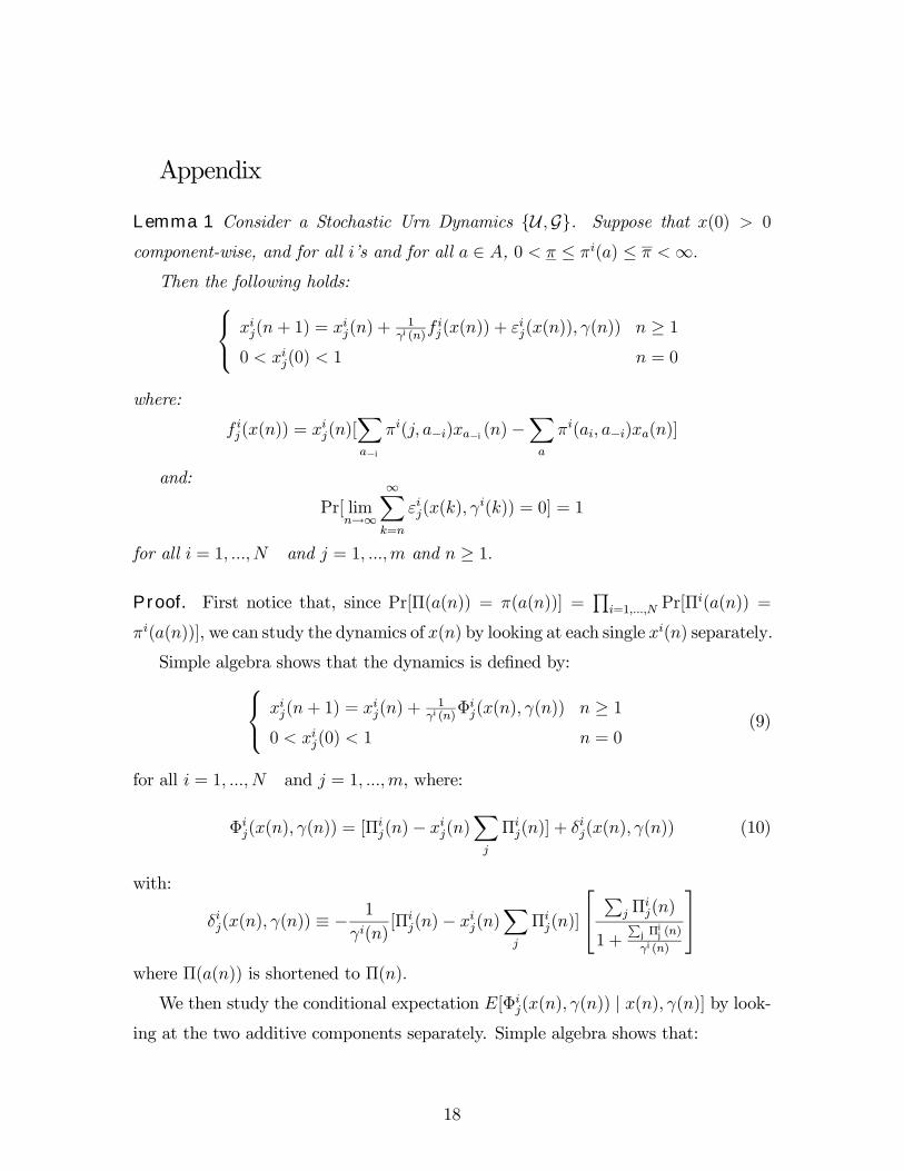
Lemma 1 Consider a Stochastic Urn Dynamics U ,G. Suppose that x(0) > 0

component-wise, and for all i’s and for all a ∈ A, 0 < π ≤ πi(a) ≤ π <∞.Then the following holds: xij(n+ 1) = x

ij(n) +

1γi(n)

f ij(x(n)) + εij(x(n)), γ(n)) n ≥ 1

0 < xij(0) < 1 n = 0

where:

f ij(x(n)) = xij(n)[

Xa−i

πi(j, a−i)xa−i(n)−

Xa

πi(ai, a−i)xa(n)]

and:

Pr[ limn→∞

∞Xk=n

εij(x(k), γi(k)) = 0] = 1

for all i = 1, ...,N and j = 1, ...,m and n ≥ 1.

Proof. First notice that, since Pr[Π(a(n)) = π(a(n))] =Qi=1,...,N Pr[Π

i(a(n)) =

πi(a(n))], we can study the dynamics of x(n) by looking at each single xi(n) separately.

Simple algebra shows that the dynamics is defined by: xij(n+ 1) = xij(n) +

1γi(n)

Φij(x(n), γ(n)) n ≥ 10 < xij(0) < 1 n = 0

(9)

for all i = 1, ..., N and j = 1, ...,m, where:

Φij(x(n), γ(n)) = [Πij(n)− xij(n)

Xj

Πij(n)] + δij(x(n), γ(n)) (10)

with:

δij(x(n), γ(n)) ≡ −1

γi(n)[Πij(n)− xij(n)

Xj

Πij(n)]

Pj Π

ij(n)

1 +P

j Πij(n)

γi(n)

where Π(a(n)) is shortened to Π(n).

We then study the conditional expectation E[Φij(x(n), γ(n)) | x(n), γ(n)] by look-ing at the two additive components separately. Simple algebra shows that:

18

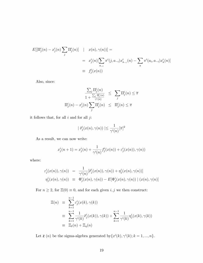
E[[Πij(n)− xij(n)Xj

Πij(n)] | x(n), γ(n))] =

= xij(n)[Xa−i

πi(j, a−i)xia−i(n)−

Xa

πi(ai, a−i)xia(n)]

≡ f ij(x(n))

Also, since: Pj Π

ij(n)

1 +P

j Πij(n)

γi(n)

≤Xj

Πij(n) ≤ π

Πij(n)− xij(n)Xj

Πij(n) ≤ Πij(n) ≤ π

it follows that, for all i and for all j:

| δij(x(n), γ(n)) |≤1

γi(n)[π]2

As a result, we can now write:

xij(n+ 1) = xij(n) +

1

γi(n)f ij(x(n)) + ε

ij(x(n)), γ(n))

where:

εij(x(n)), γ(n)) =1

γi(n)[δij(x(n)), γ(n)) + η

ij(x(n), γ(n))]

ηij(x(n), γ(n)) ≡ Φij(x(n), γ(n))− E[Φij(x(n), γ(n)) | (x(n), γ(n)]

For n ≥ 2, for Ξ(0) ≡ 0, and for each given i, j we then construct:

Ξ(n) ≡n−1Xk=1

εij(x(k), γ(k))

≡n−1Xk=1

1

γi(k)δij(x(k)), γ(k)) +

n−1Xk=1

1

γi(k)ηij(x(k), γ(k))

≡ Ξδ(n) + Ξη(n)

Let z(n) be the sigma-algebra generated byxi(k), γi(k); k = 1, ..., n.

19

Note that:

Ξδ(n+ 1) = Ξδ(n) +1

γi(n)δij(x(n), γ(n))

Ξη(n+ 1) = Ξη(n) +1

γi(n)ηij(x(n), γ(n))

and since by construction, δij is bounded as in eq. (4), it follows that:

Ξδ(n+ 1) ≤ Ξδ(n) +π2

γi(n)2≤ Ξδ(n) + π2

gi(n)2

where gi(n) = γi(0) + nπ is deterministic.

Hence, we can construct an auxiliary stochastic process:

Z(n) ≡ Ξδ(n) + π2Xk≥n

1

gi(k)2

where the series of which in the second term converges, and show that this is a

supermartingale relative to z(n). In fact:

E[Z(n+ 1) | z(n)] =

= E[Ξδ(n+ 1) | z(n)] + π2Xk≥n+1

1

gi(k)2

≤ Ξδ(n) + π2 1

gi(n)2+ π2

Xk≥n+1

1

gi(k)2

= Ξδ(n) + π2Xk≥n

1

gi(k)2≡ Z(n)

By the convergence theorem for supermartingales, there exists a random variable

Z(∞) and, for n → ∞, Z(n) converges pointwise to Z(∞) with probability one.Hence, also Ξδ(n) converges to Ξδ(∞) with probability one.With regard to Ξη(n), since E[ηij(x(n), γ(n)) | z(n)] = 0, Ξη(n) is a quadratically

integrable martingale relative to z(n). Hence (see for ex. Karlin and Taylor (1975),

p. 282), there exists a random variable Ξη(∞) and Ξη(n)→ Ξη(∞) for n→∞ a.s..

Since Ξ(∞)− Ξ(n) ≡P∞k=n ε

ij(x(k), γ

i(k)), the assert follows.

20

Remark 2 Let Ω∗ be a subspace of the sample space of the process x(n), γ(n) suchthat the assumptions of Lemma 1 hold. For a given initial condition [x(0), γ(0)], con-

sider a fixed realization ω∗ ∈ Ω∗ and the corresponding sequence x(n,ω∗), γ(n,ω∗).Any component of the vector γ(n,ω∗) ≡ [γi(n,ω∗), i = 1, 2, ..., N ], regarded as a

sequence over n, satisfies the following:

0 <1

γi(0) + nπ≤ 1

γi(n,ω∗)≤ 1

γi(0) + nπ

Hence:

limn→∞

1

γi(n,ω∗)= 0

∞Xn=0

1

γi(n,ω∗)=∞

∞Xn=0

1

(γi(n,ω∗))2<∞

As a result, any sequence γi(n,ω∗), n > 0 satisfies Assumption 2, for any i and forany realization ω∗.

Lemma 2 Consider the stochastic process Ug,G under the assumptions of Lemma1. Define the number m(n,∆t) such that

limn→∞

m(n,∆t)−1Xk=n

1

g(k)= ∆t

Assume that, for ρ = ρ(x0) > 0 and sufficiently small, x(n) ∈ B(x0, ρ) = x :|x− x0| < ρ. Then there exists a value ∆t0(x0, ρ) and a number N0 = N0(x0, ρ) suchthat, for ∆t < ∆t0 and n > N0, x(k) ∈ B(x0, ρ) for all n ≤ k ≤ m(n,∆t).

Proof. By Lemma 1, for j(n) ≥ n+ 1, the process Ug,G can be re-written as:

x(j(n)) = x(n) +

j(n)−1Xs=n

1

g(s)f(x0) +

j(n)−1Xs=n

1

g(s)[f(x(s))− f(x0)] +

j(n)−1Xs=n

ε(x(s)), g(s))

and an upper bound for x(j(n)) can be constructed as follows.

21

Since the function f is Lipschitz in x:

j(n)−1Xs=n

1

g(s)|f(x(s))− f(x0)| ≤ L max

n≤k≤j(n)−1| x(k)− x0 |

j(n)−1Xs=n

1

g(s)

where L is global Lipschitz constant. Hence, by letting ∆t(n, j(n)) ≡j(n)−1Ps=n

g(s)−1 we

obtain:

|x(j(n))| ≤ |x(n)|+∆t(n, j(n)) | f(x0) | +

+∆t(n, j(n))L maxn≤k≤j(n)−1

| x(k)− x0 | + (11)

+

¯¯j(n)−1Xs=n

ε(x(s), g(s))

¯¯

As for the last term, from Lemma 1 we know that, for all α > 0 there exists an

n = n(α) such that for all n > n(α) with probability one:¯¯j(n)−1Xs=n

ε(x(s), g(s))

¯¯ ≤ α

since these are differences between converging martingales.

Now consider j(n) = m(n,∆t), where m is such that limn→∞∆t(n,m(n,∆t)) =

∆t. Note that the numberm is finite for any n and for any∆t <∞, sincePs g(s)−1 =

∞ andP

s g(s)−2 < ∞ by assumption. Denote

¯Pj(n)−1s=n ε(x(s), g(s))

¯by α(n) and

suppose x(k) ∈ B(x0, 2ρ) for all n ≤ k ≤ m(n,∆t)− 1.Inequality (11) states that:

|x(m)| ≤ |x(n)|+∆t | f(x0) | +∆t2ρL+ α(n)

Hence:

|x(m)− x0| ≤ |x(m)− x(n)|+ |x(n)− x0|≤ ∆t |f(x0)|+∆t2Lρ+ α(n) + ρ

22

and as a result, we can choose N0(ρ) = n(ρ2) such that, for all n > N0,α(n) <

ρ2

and ∆t0(x0, ρ) = ρ2(|f(x0)|+2Lρ)−1 > 0 and show that, for all ∆t < ∆t0 and n > N0 :

|x(m)− x0| ≤ ρ

2+ρ

2+ ρ = 2ρ

Hence if x(k) ∈ B(x0, 2ρ) for all n ≤ k ≤ m − 1, this implies that also x(m) ∈B(x0, 2ρ). By induction it then follows that x(k) remains in B(x0, 2ρ) also for all k upto m(n,∆t)− 1.

Lemma 3 Beyond the assumptions of Lemma 2, suppose that the system of ODE (4)

satisfies property (7) on a compact set D ⊆ ∆. Suppose x(nl) ∈ D with probability

one, and xD0 (l) ∈ D.Then,

if¯xD0 (l)− x(nl)

¯ ≤ ε, also ¯xD0 (l + 1)− x(nl+1)¯ ≤ εfor λε

2L≤ ∆tl ≤ 3λε

2L, where 0 < λ < 1, L is the Lipschitz constant of f(.) on D, and

0 < ε < ε = minq(6λ2)−14ρL, (3λ)−12L∆t0 with ∆t0 = infx∈D,ρ=ρ(x)∆t0(x, ρ) > 0

defined in Lemma 2.

Proof. Let I = nl | l ≥ 0 be a collection of indices such that 0 < n0 < n1 < .... <nl< nl+1 < ..... and let ∆tl = tl+1 − tl, with tl =

nl−1Pk=n0

g(k)−1. Lemma 1 states that

the value of the process at time nl+1 is given by:

x(nl+1) = x(nl) +∆tlf(x(nl)) + α(nl)

and Lemma 2 shows that, for ∆tl small and nl large, α(nl) < ρ/2, meaning that

if the process is started at x(nl), it stays close to it for some time.

Solve the system of differential equations (4) from tl to tl + ∆tl Since f(.) is

Lipschitz continuous: ¯xD(t+∆t, t, x)− (x+∆tf(x))¯ ≤ L∆t2

where xD(t+∆t, t, x) denotes the solution at time t+∆t, when the initial condition

is taken to be x at time t and L is a constant.

23

Now take x(nl) = x and compute the distance between the stochastic process at

step nl+1, x(nl+1), and the differential equation at time tl+1, with initial condition x

at time tl, xD(tl+1, tl, x) shortened to xDl (l + 1) :¯x(nl+1)− xDl (l + 1)

¯=

¯x(nl) +∆tlf(x(nl)) + α(nl)− xDl (l + 1)

¯≤ L∆t2 + α(nl)

As a result:¯xD0 (l + 1)− x(nl+1)

¯ ≤ ¯xD0 (l + 1)− xDl (l + 1)

¯+¯xDl (l + 1)− x(nl+1)

¯≤ ¯

xD0 (l + 1)− xDl (l + 1)¯+ L∆t2l + α(nl) (12)

where the first term is the distance between two trajectories of the ODE, one started

at x(n0) and one at x(nl) at time t0 and tl respectively, and the second term is the

distance between the ODE and the stochastic process at time tl+1. We know from

Lemma 2 that the last two terms on the RHS of (12) can be made arbitrarily small

by an appropriate choice of ∆tl and nl. We also know that, if the two trajectories

of which in the first term of the RHS of (12) converge, their distance will become

increasingly small. An assumption that is sufficient to establish the result that follows

requires: ¯xD(t+∆t, t, x+∆x)− xD(t+∆t, t, x)¯ ≤ (1− λ∆t) |∆x| (13)

with 0 < λ < 1. If property (7) holds, then:¯xD0 (l + 1)− xDl (l + 1)

¯ ≤ (1− λ∆tl) ¯xD0 (l)− x(nl)¯and as a result, inequality (12) can be rewritten as:¯

xD0 (l + 1)− x(nl+1)¯ ≤ (1− λ∆tl) ¯xD0 (l)− x(nl)¯+ L∆t2l + α(nl) (14)

We can now show that, if x(nl) lies in an ε-neighbourhood of the trajectory of the

ODE, so will x(nl+1), for a suitable choice of ε and ∆t.

Under the assumptions of this Lemma, inequality (14) yields:¯xD0 (l + 1)− x(nl+1)

¯ ≤ (1− λ∆tl)ε+ L∆t2l + α(nl)24

By Lemma 2 α(nl) < r(ε) ≡ λ2ε234L

< ρ2, which holds for 0 < ε <

q4ρL6λ2 as assumed.

Hence:

(1− λ∆tl)ε+ L∆t2l + α(nl) ≤ ε− λ∆tlε+ L∆t2l +λ2ε23

4L

= ε+ L

·µ∆tl − λε

2L

¶µ∆tl − 3λε

2L

¶¸< ε

as stated.

We also need to show that for λε(2L)−1 ≤ ∆tl ≤ 3λε(2L)−1, ∆tl also satisfies

Lemma 2, i.e. ∆tl < ∆t0(x, ρ) for all x ∈ D. The radius ρ depends on x and is ameasure of how fast f(x) changes in a neighbourhood of x. Since f(x) is Lipschit z

and D is compact, this radius will have a positive lower bound, as x moves in D. Let

this be ρ > 0. Hence:

∆t0 = infx∈D

∆t0(x) ≡ infx∈D

µρ

2[|f(x)|+ 2Lρ]¶> 0

and since ε < (3λ)−12L∆t0 by assumption, the assert follows.

Proof of Theorem 1

To proof the Theorem we need to estimate the probability that Lemma 2 holds

for all nl ∈ I. To this aim note that:

Pr

·supnl∈I

¯x(nl)− xD0 (l)

¯ ≤ ε¸ = Pr ·supnl∈I

α(nl) < r(ε)

¸where, as before xD0 (l) ≡ xD(tl, t0, x(n0)).From Lemma 2:

α(nl) ≡ |ε(x(nl), g(nl))| ≡¯¯nlX

k=n0

ε(x(k), g(k))−nl−1Xk=n0

ε(x(k), g(k))

¯¯

and from Lemma 1:

E[εij(x(k), g(k)] ≤π2

g(k)2

As a result:

α(nl) ≤√NM sup

isupjεij(x(k), g(k) ≤

√NM

π2

g(nl)2

E[α(nl)] ≤√NM

π2

g(nl)2

25

By Chebyshev’s inequality:

Pr [α(nl) > r(ε)] ≤√NM

r(ε)

π2

g(nl)2

Hence:

Pr[α(nl) ≥ r(ε);nl > n0, nl ∈ I] ≤ C

ε2

NXj=n0

1

g(j)2

where C = (3λ2)−14L√NMπ2 since r(ε) ≡ (4L)−1λ2ε2. In the statement of the

theorem n = N0(ρ), defined in Lemma 2 and ε = min(3λ)−12L,p(6λ)−14ρL asfrom Lemma 3.

Proof of Remark 1

To prove the statement we need to show that every strict Nash equilibrium satisfies

condition (7), i.e.:¯xD(t+∆t, t, x+∆x)− xD(t+∆t, t, x)¯ ≤ (1− λ∆t) |∆x| (15)

This condition holds if the system of ODE (4) admits the following quadratic Ljapunov

function (see, for example, Ljung (1977)):

V (∆x, t) = |∆x|2 (a)

d

dtV (∆x, t) < −C |∆x|2 C > 0 (b)

Suppose x∗ is a strict Nash equilibrium and w.l.g. let x∗ = 0. Consider the

linearization of the system (4) around x∗ = 0 :

d

dtxD(t) = Ax+ g(x)

where A ≡ Df(x)|x∗=0 denotes the Jacobian matrix of f(x) at x∗ and limx→0 g(x)|x| = 0.

From Ritzberger and Weibull (1995), Proposition 2, we know that a Nash equilibrium

is asymptotically stable in the replicator dynamics if and only if it is strict. Hence

we also know that all the eigenvalues of A at x∗ have negative real part and (see for

example Walter (1998), p. 321) we can consider the following scalar product in <Nm:

hx, yi =∞Z0

(eAtx, eAty)dt

26

and choose:

V (x, t) = hx, xi

which satisfies condition (a). The scalar product (4) also satisfies condition (b), since:

d

dtV (x, t) ≤ − |x|2 + 2 hx, g(x)i ≤ − |x|2 + 2

phx, xi

phg(x), g(x)i

By the equivalence of norms in <N , there exists a c > 0 s.t.phx, xi ≤ c |x|. For

r > 0, consider an open ball Br = x ∈ ∆ : |x| < r such that Br ⊂ D and

|g(x)| ≤ (1/(4c2)) |x| in Br. Then:d

dtV (x, t) ≤ − |x|2 + 2c2 |x| |g(x)| ≤ −1

2|x|2 ≤ − 1

2c2V (x, t) in Br

which shows that condition (b) holds.

27

Notes1A result along these lines is also obtained in Beggs (2001), where the author shows that strategies

converge in constant-sum games with a unique equilibrium and in 2-by-2 games also if they are mixed.

2Rustichini’s result is of interest as it also indirectly complements the literature on non-linear

urn processes (see for example Arthur et al. (1988a), Pemantle (1990) and the application of the

latter in Benaim and Hirsh (1999), Theorem 5.1) by providing sufficient conditions for attainability

and unattainability of fixed points at the boundary of the simplex.

3We hereby assume that each player’s action space has exactly the same cardinality (i.e. m).

This is purely for notational convenience.

4One immediate relation between Börgers and Sarin (1997)’s model and the one we study, can

be drawn as follows. Let f(x,Π) denote a standard discrete time system of replicator equations

for an underlying game with strictly positive payoff functions Π. At step n of the repetition of the

game, suppose γi(n) = n for all is and consider the following renormalization of the payoffs of the

game: eΠ ≡ Π

n+Π: A→ (0, 1)

These renormalized payoffs clearly satisfy Borgers and Sarin’s assumption; hence their result of

Section 2 applies and the expected motion of the system (2), conditional upon step n being reached

is given by:

E[x(n+ 1) | x(n) = x, γ(n) = n] = x+ f(x, eΠ)i.e. is given by a replicator dynamics in the renormalized variables eΠ. It is worth noticing

that, since asymmetric replicator dynamics are not invariant under positive affine transformations

of payoffs, in general, the solution orbits of f(x, eΠ) differ from those of f(x,Π). However, since:

Π

n+Π=Π

n− Π2

n2 + nΠ

the renormalization is the sum of a °(n−1) component that affects all payoffs for all players in

the same fashion, and hence only alters the speed at which the state moves along the orbits, and

a °(n−2) component which is instead payoff specific. Hence, up to an °(n−2) error term, the

expected increment of the process, x, given x(n), is given by n times f(x,Π), i.e.:

E[xi(n+ 1) | x(n) = x, γ(n) = n] = xi +1

nf i(x,Π) +°(n−2)

5If, for any profile of actions a, 0 < π ≤ πi(a) ≤ π <∞, then the random variable γi(n) is such

that:

γi(0) + nπ ≤ γi(n) ≤ γi(0) + nπ

28

for any n, with probability one.

6Convergence in the sense that:

infx∈DR

|x(t)− x|→ 0 for t→∞

29

REFERENCES

Arthur, W.B. (1993), “On designing economic agents that behave like human

agents," Journal of Evolutionary Economics, 3, 1-22.

Arthur, W.B. Yu., M. Ermoliev and Yu. Kaniovski (1987), “Non-linear Urn

Processes: Asymptotic Behavior and Applications," mimeo, IIASAWP-87-85.

Arthur, W.B. Yu., M. Ermoliev and Yu. Kaniovski (1988), “Non-linear Adap-

tive Processes of Growth with General Increments: Attainable and Unattainable

Components of Terminal Set.," mimeo, IIASA WP-88-86.

Beggs, A.W. (2001), “On the Convergence of Reinforcement Learning.," mimeo,

Oxford University.

Benaim, M. (1999), “Dynamics of Stochastic Approximation, Le Seminaire de

Probabilite’, Springer Lecture Notes in Mathematics.

Benaim, M. and M. Hirsch (1999a), “Stochastic Approximation algorithms with

constant step size whose average is cooperative," Annals of Applied Probability,

9, 216-241.

Benaim, M. and M. Hirsch (1999b), “Mixed Equilibria and dynamical systems

arising from fictitious play in perturbed games," Games and Economic Behav-

ior, 29, 36-72.

Benaim, M and J. Weibull (2000), “Deterministic Approximation of Stochastic

Evolution in Games," mimeo, Stockholm School of Economics.

Benveniste, A., Metivier, M. and P. Priouret (1990), “Adaptive Algorithms

and Stochastic Approximation, . Springer-Verlag.

Binmore, K., Samuelson, L. and R. Vaughan (1995), “Musical Chairs: Mod-

elling noisy evolution," Games and Economic Behavior, 11, 1-35.

30

Binmore, K. and L. Samuelson (1997), “Muddling through: Noisy equilibrium

selection," Journal of Economic Theory, 74, 235-265.

Binmore, K. and L. Samuelson (1999), “Evolutionary Drift and Equilibrium

Selection," Review of Economic Studies, 66, 363-393.

Börgers, T. and R. Sarin (1997), “Learning Through Reinforcement and Repli-

cator Dynamics," Journal of Economic Theory, 77, 1-14.

Boylan R. (1995), “Continuous approximation of dynamical systems with ran-

domly mathced individuals," Journal of Economic Theory, 66, 615-625.

Bush, R.R. and F. Mosteller (1955), “Stochastic Models for Learning, . New

York: Wiley.

Camerer, C. and T.H. Ho (1999), “Experience-Weighted Attraction Learning

in Normal Form Games," Econometrica, 67(4), 827-874.

Corradi V. and R. Sarin (1999), “Continuous approximations of stochastic evo-

lutionary game dynamics," Journal of Economic Theory„ ?, ?-?.

Cross, J.G. (1973), “A Stochastic LearningModel of Economic Behavior," Quaterly

Journal of Economics, 87, 239-266.

Cross, J.G. (1983), “A Theory of Adaptive Economic Behavior, . Cambridge:

Cambridge University Press.

Erev, I. and A.E. Roth (1998), “Predicting How People Play Games: Rein-

forcement Learning in Experimental Games with Unique, Mixed Strategy Equi-

libria," American Economic Review, 88(4), 848-881.

Feltovich, N. (2000), “Reinforcement-based vs. belief-based learning models in

experimental asymmetric information games," Econometrica, 68, 605-641.

Fudenberg D. and D. Kreps (1993), “Learning Mixed Equilibria," Games and

economic Behavior, 5, 320-367.

31

Fudenberg D. and D. Levine (1995), “Consistency and Cautious Fictitious Play,"

Journal of Economic Dynamic and Control, 19, 1065-1089.

Fudenberg D. and D. Levine (1998), “Theory of Learning in Games, . MIT

Press.

Hill, B.M., Lane, D. and W. Sudderth (1980), “A strong law for some gen-

eralized urn processes," The Annals of Probability, 8, 214-226.

Hofbauer J. and K. Sigmund (1988), “The Thoery of Evolution and Dynamical

Systems, . Cambridge University Press.

Hopkins, E. (2000), “Two competing models of how people learn in games,"

mimeo, University of Edinburg (fortcoming in Econometrica).

Kandori, M., G. Mailath and R. Rob (1993), “Learning, Mutations, and Long

Run Equilibria in Games," Econometrica, 61, 29-56.

Kaniovski Y. and P. Young (1995), “Learning dynamics in games with sto-

chastic perturbations," Games and Economic Behavior, 11, 330-363.

Karlin, S. and H. Taylor (1981), “A Second Course in Stochastic Processes, .

Academic Press.

Ljung, L. (1977), “Analysis of recursive stochastic algorithms," IEEE Trans.

Automatic Control, AC22, 551-575.

Ljung, L. (1978), “Strong Convergence of a Stochastic Approximation Algorithm,"

Annals of Probability, 6, 680-696.

Mookherjee, D. and B. Sopher (1997), “Learning and decision costs in exper-

imental constant sum games," Games and Economic Behavior, 19, 97-132.

Pemantle, R. (1990), “Non-convergence to unstable points in urn models and

stochastic approximation," The Annals of Probability, 18, 698-712.

32

Posh, M. (1997), “Cycling in a stochastic learning algorithm for normal form

games," Journal of Evolutionary Dynamics, 7, 193-207.

Ritzberger K. and J. Weibull (1995), “Evolutionary Selection in normal form

games," Econometrica, 63, 1371-1399.

Roth, A. and I. Erev (1995), “Learning in Extensive Form Games: Experimen-

tal Data and Simple Dynamic Models in the Intermediate Term," Games and

Economic Behavior, 8(1), 164-212.

Rustichini, A. (1999), “Optimal Properties of Stimulus-Response Learning Mod-

els," Games and Economic Behavior, 29, 244-273.

Sarin, R. and F. Vahid (1998), “Predicting how people play games: a procedu-

rally rational model of choice.," mimeo, Texas AM University.

Taylor, P. (1979), “Evolutionary stable strategies with two types of player,"

Journal of Applied Probability, 16, 76-83.

Young, H. P. (1993), “The Evolution of Conventions," Econometrica, 61, 57-84.

Walter, W. (1998), “Ordinary Differential Equations, . Springer-Verlag.

Weibull J. (1995), “Evolutionary Game Theory, . MIT Press.

33