Embed Size (px)
Citation preview
Reinforcement Learning
Inverse Reinforcement Learning
LfD, imitation learning/behavior cloning, apprenticeship learning, IRL.
Hung NgoMLR Lab, University of Stuttgart
Outline
• Learning from Demonstrations (LfD)
• Behavioral Cloning/Imitation Learning
• Inverse Reinforcement Learning (IRL) Algorithms
2/14
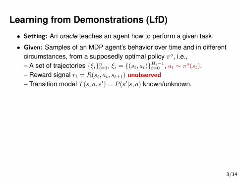
Learning from Demonstrations (LfD)
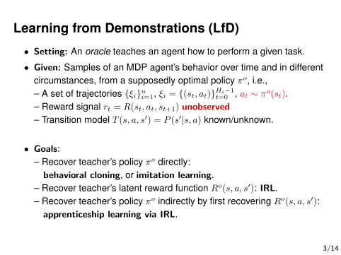
• Setting: An oracle teaches an agent how to perform a given task.
• Given: Samples of an MDP agent’s behavior over time and in differentcircumstances, from a supposedly optimal policy πo, i.e.,– A set of trajectories {ξi}ni=1, ξi = {(st, at)}Hi−1
t=0 , at ∼ πo(st).– Reward signal rt = R(st, at, st+1) unobserved
– Transition model T (s, a, s′) = P (s′|s, a) known/unknown.
• Goals:– Recover teacher’s policy πo directly:
behavioral cloning, or imitation learning.– Recover teacher’s latent reward function Ro(s, a, s′): IRL.– Recover teacher’s policy πo indirectly by first recovering Ro(s, a, s′):
apprenticeship learning via IRL.
3/14
Learning from Demonstrations (LfD)
• Setting: An oracle teaches an agent how to perform a given task.
• Given: Samples of an MDP agent’s behavior over time and in differentcircumstances, from a supposedly optimal policy πo, i.e.,– A set of trajectories {ξi}ni=1, ξi = {(st, at)}Hi−1
t=0 , at ∼ πo(st).– Reward signal rt = R(st, at, st+1) unobserved
– Transition model T (s, a, s′) = P (s′|s, a) known/unknown.
• Goals:– Recover teacher’s policy πo directly:behavioral cloning, or imitation learning.
– Recover teacher’s latent reward function Ro(s, a, s′): IRL.– Recover teacher’s policy πo indirectly by first recovering Ro(s, a, s′):apprenticeship learning via IRL.
3/14
Behavioral cloning
• Formulated as a supervised-learning problem– Given training data {ξi}ni=1, ξi = {(st, at)}Hi−1
t=0 , at ∼ πo(st).– Learn policy mapping πo : S → A.– Solved using SVM, (deep) ANN, etc.
• Behavioral cloning/IL: can only mimic the trajectory of the teacher,– no transfer w.r.t. task (e.g., env. changed but similar goals),– may fail in non-Markovian environments
(e.g. in driving; sometimes states from several time-steps needed).
• IRL vs. behavioral cloning: Ro vs. πo. Why not recover V πo
instead?– reward function is more succint (easily generalizable/transferrable)– values are trajectory dependent
4/14
Why IRL?
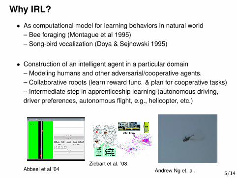
• As computational model for learning behaviors in natural world– Bee foraging (Montague et al 1995)– Song-bird vocalization (Doya & Sejnowski 1995)
• Construction of an intelligent agent in a particular domain– Modeling humans and other adversarial/cooperative agents.– Collaborative robots (learn reward func. & plan for cooperative tasks)– Intermediate step in apprenticeship learning (autonomous driving,driver preferences, autonomous flight, e.g., helicopter, etc.)
Abbeel et al ’04Ziebart et al. ’08
Andrew Ng et. al.
5/14
Why IRL?
• As computational model for learning behaviors in natural world– Bee foraging (Montague et al 1995)– Song-bird vocalization (Doya & Sejnowski 1995)
• Construction of an intelligent agent in a particular domain– Modeling humans and other adversarial/cooperative agents.– Collaborative robots (learn reward func. & plan for cooperative tasks)– Intermediate step in apprenticeship learning (autonomous driving,driver preferences, autonomous flight, e.g., helicopter, etc.)
Abbeel et al ’04Ziebart et al. ’08
Andrew Ng et. al. 5/14

Example: Urban Navigation
picture from a tutorial of Pieter Abbeel.
6/14
IRL Formulation #1: Small, Discrete MDPs
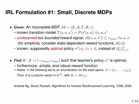
• Given: An incomplete MDPM = 〈S,A, T,R, γ〉.– known transition model T (s, a, s′) = P (s′|s, a),∀s, a, s′
– unobserved but bounded reward signal, |R(s, a, s′)| ≤ rmax,∀s, a, s′
(for simplicity, consider state-dependent reward functions, R(s))– known, supposedly optimal policy πo(s),∀s ∈ S, instead of {ξi}ni=1.
• Find R : S → [−rmax, rmax] such that teacher’s policy πo is optimal,– furthermore: simple, and robust reward function– Notes: in the following we fix an enumeration on the state space: S = {s1, . . . , s|S|}.
Then R is a column vector in R|S|, with Ri = R(si).
Andrew Ng, Stuart Russell: Algorithms for Inverse Reinforcement Learning. ICML 2000.
7/14
IRL Formulation #1: Small, Discrete MDPs
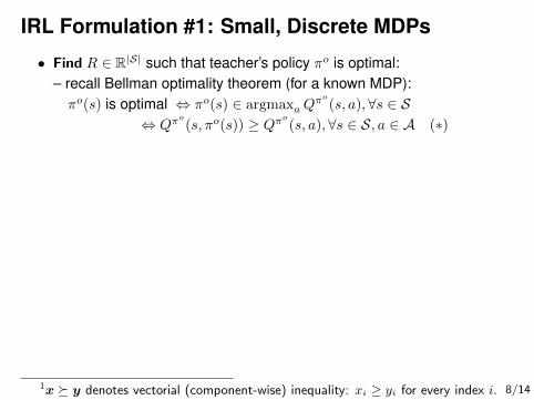
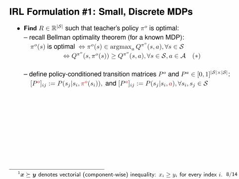
• Find R ∈ R|S| such that teacher’s policy πo is optimal:– recall Bellman optimality theorem (for a known MDP):πo(s) is optimal ⇔ πo(s) ∈ argmaxaQ
πo
(s, a),∀s ∈ S⇔ Qπ
o
(s, πo(s)) ≥ Qπo
(s, a),∀s ∈ S, a ∈ A (∗)
– define policy-conditioned transition matrices P o and P a ∈ [0, 1]|S|×|S|:[P o]ij := P (sj |si, πo(si)), and [P a]ij := P (sj |si, a),∀si, sj ∈ S
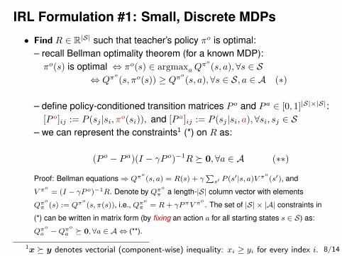
– we can represent the constraints1 (*) on R as:
(P o − P a)(I − γP o)−1R � 0,∀a ∈ A (∗∗)
Proof: Bellman equations⇒ Qπo(s, a) = R(s) + γ
∑s′ P (s′|s, a)V π
o(s′), and
V πo
= (I − γP o)−1R. Denote by Qπo
π a length-|S| column vector with elements
Qπo
π (s) := Qπo(s, π(s)), i.e., Qπ
o
π = R+ γPπV πo
. The set of |S| × |A| constraints in
(*) can be written in matrix form (by fixing an action a for all starting states s ∈ S) as:
Qπo
o −Qπo
a � 0, ∀a ∈ A ⇔ (**).
1x � y denotes vectorial (component-wise) inequality: xi ≥ yi for every index i. 8/14
IRL Formulation #1: Small, Discrete MDPs
• Find R ∈ R|S| such that teacher’s policy πo is optimal:– recall Bellman optimality theorem (for a known MDP):πo(s) is optimal ⇔ πo(s) ∈ argmaxaQ
πo
(s, a),∀s ∈ S⇔ Qπ
o
(s, πo(s)) ≥ Qπo
(s, a),∀s ∈ S, a ∈ A (∗)
– define policy-conditioned transition matrices P o and P a ∈ [0, 1]|S|×|S|:[P o]ij := P (sj |si, πo(si)), and [P a]ij := P (sj |si, a),∀si, sj ∈ S
– we can represent the constraints1 (*) on R as:
(P o − P a)(I − γP o)−1R � 0,∀a ∈ A (∗∗)
Proof: Bellman equations⇒ Qπo(s, a) = R(s) + γ
∑s′ P (s′|s, a)V π
o(s′), and
V πo
= (I − γP o)−1R. Denote by Qπo
π a length-|S| column vector with elements
Qπo
π (s) := Qπo(s, π(s)), i.e., Qπ
o
π = R+ γPπV πo
. The set of |S| × |A| constraints in
(*) can be written in matrix form (by fixing an action a for all starting states s ∈ S) as:
Qπo
o −Qπo
a � 0, ∀a ∈ A ⇔ (**).
1x � y denotes vectorial (component-wise) inequality: xi ≥ yi for every index i. 8/14
IRL Formulation #1: Small, Discrete MDPs
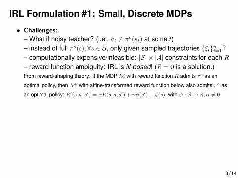
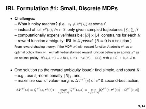
• Challenges:
– What if noisy teacher? (i.e., at 6= πo(st) at some t)– instead of full πo(s),∀s ∈ S, only given sampled trajectories {ξi}ni=1?– computationally expensive/infeasible: |S| × |A| constraints for each R– reward function ambiguity: IRL is ill-posed! (R = 0 is a solution.)From reward-shaping theory: If the MDPM with reward function R admits πo as an
optimal policy, thenM′ with affine-transformed reward function below also admits πo as
an optimal policy: R′(s, a, s′) = αR(s, a, s′) + γψ(s′)− ψ(s), with ψ : S → R, α 6= 0.
• One solution (to the reward ambiguity issue): find simple, and robust R,– e.g., use `1-norm penalty ||R||1, and– maximize sum of value-margins ∆V π
o
(s) of πo & second-best action,
∆V πo(s) = Qπ
o(s, πo(s))− max
a6=πo(s)Qπ
o(s, a) = min
a6=πo(s)[Qπ
o(s, πo(s))−Qπ
o(s, a)]
9/14
IRL Formulation #1: Small, Discrete MDPs
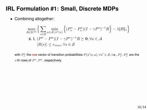
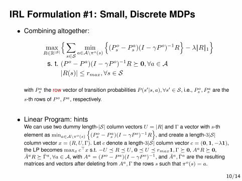
• Combining altogether:
maxR∈R|S|
{∑s∈S
mina∈A\πo(s)
{(P os − P as )(I − γP o)−1R
}− λ||R||1
}s. t. (P o − P a)(I − γP o)−1R � 0,∀a ∈ A
|R(s)| ≤ rmax,∀s ∈ S
with Pas the row vector of transition probabilities P (s′|s, a), ∀s′ ∈ S, i.e., P os , Pas are the
s-th rows of P o, Pa, respectively.
• Linear Program: hintsWe can use two dummy length-|S| column vectors U = |R| and Γ a vector with s-thelement as mina∈A\πo(s)
{(P os − Pas )(I − γP o)−1R
}, and create a length-3|S|
column vector x = (R,U,Γ). Let c denote a length-3|S| column vector c = (0,1,−λ1),the LP becomes maxx c>x s.t. −U � R � U , 0 � U � rmax1,Γ � 0, AaR � 0,AaR � Γa, ∀a ∈ A, with Aa = (P o − Pa)(I − γP o)−1, and Aa, Γa are the resultingmatrices and vectors after deleting from Aa,Γ the rows s such that πo(s) = a.
10/14
IRL Formulation #1: Small, Discrete MDPs
• Combining altogether:
maxR∈R|S|
{∑s∈S
mina∈A\πo(s)
{(P os − P as )(I − γP o)−1R
}− λ||R||1
}s. t. (P o − P a)(I − γP o)−1R � 0,∀a ∈ A
|R(s)| ≤ rmax,∀s ∈ S
with Pas the row vector of transition probabilities P (s′|s, a), ∀s′ ∈ S, i.e., P os , Pas are the
s-th rows of P o, Pa, respectively.
• Linear Program: hintsWe can use two dummy length-|S| column vectors U = |R| and Γ a vector with s-thelement as mina∈A\πo(s)
{(P os − Pas )(I − γP o)−1R
}, and create a length-3|S|
column vector x = (R,U,Γ). Let c denote a length-3|S| column vector c = (0,1,−λ1),the LP becomes maxx c>x s.t. −U � R � U , 0 � U � rmax1,Γ � 0, AaR � 0,AaR � Γa, ∀a ∈ A, with Aa = (P o − Pa)(I − γP o)−1, and Aa, Γa are the resultingmatrices and vectors after deleting from Aa,Γ the rows s such that πo(s) = a.
10/14
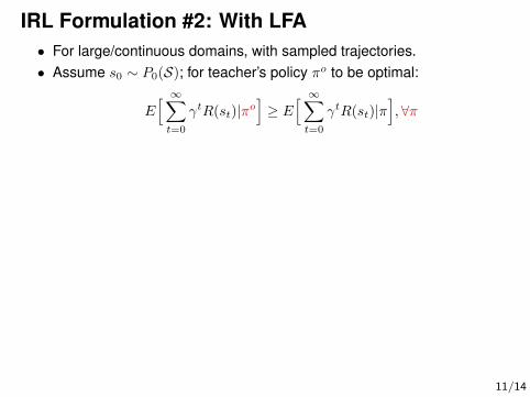
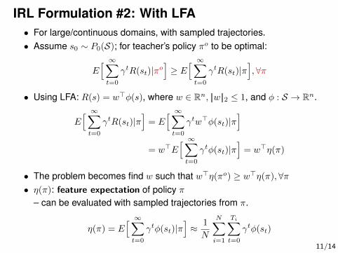
IRL Formulation #2: With LFA• For large/continuous domains, with sampled trajectories.• Assume s0 ∼ P0(S); for teacher’s policy πo to be optimal:
E[ ∞∑t=0
γtR(st)|πo]≥ E
[ ∞∑t=0
γtR(st)|π],∀π
• Using LFA: R(s) = w>φ(s), where w ∈ Rn, ||w||2 ≤ 1, and φ : S → Rn.
E[ ∞∑t=0
γtR(st)|π]
= E[ ∞∑t=0
γtw>φ(st)|π]
= w>E[ ∞∑t=0
γtφ(st)|π]
= w>η(π)
• The problem becomes find w such that w>η(πo) ≥ w>η(π),∀π• η(π): feature expectation of policy π
– can be evaluated with sampled trajectories from π.
η(π) = E[ ∞∑t=0
γtφ(st)|π]≈ 1
N
N∑i=1
Ti∑t=0
γtφ(st)
11/14

Apprenticeship learning: Literature
Pieter Abbeel, Andrew Ng: Apprenticeship learning via inverse RL. ICML’04Pieter Abbeel et al.: An Application of RL to Aerobatic Helicopter Flight. NIPS’06.Ratliff, Nathanet al., “Maximum margin planning.” ICML’06Ziebart, Brian D., et al. Maximum Entropy Inverse Reinforcement Learning. AAAI’08Adam Coates et al.. Apprenticeship learning for helicopter control. Commun. ACM’09
12/14
Apprenticeship learning via IRL: Max-margin
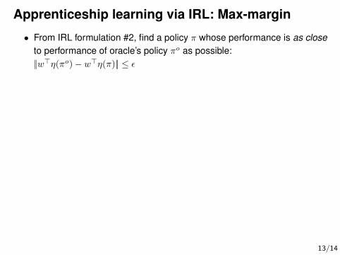
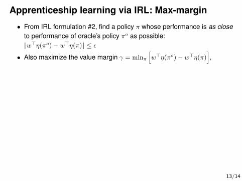
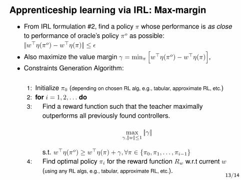
• From IRL formulation #2, find a policy π whose performance is as closeto performance of oracle’s policy πo as possible:||w>η(πo)− w>η(π)|| ≤ ε
• Also maximize the value margin γ = minπ
[w>η(πo)− w>η(π)
],
• Constraints Generation Algorithm:
1: Initialize π0 (depending on chosen RL alg, e.g., tabular, approximate RL, etc.)2: for i = 1, 2, . . . do3: Find a reward function such that the teacher maximally
outperforms all previously found controllers.
maxγ,||w||≤1
||γ||
s.t. w>η(πo) ≥ w>η(π) + γ,∀π ∈ {π0, π1, . . . , πi−1}4: Find optimal policy πi for the reward function Rw w.r.t current w
(using any RL algs, e.g., tabular, approximate RL, etc.).
13/14
Apprenticeship learning via IRL: Max-margin
• From IRL formulation #2, find a policy π whose performance is as closeto performance of oracle’s policy πo as possible:||w>η(πo)− w>η(π)|| ≤ ε
• Also maximize the value margin γ = minπ
[w>η(πo)− w>η(π)
],
• Constraints Generation Algorithm:
1: Initialize π0 (depending on chosen RL alg, e.g., tabular, approximate RL, etc.)2: for i = 1, 2, . . . do3: Find a reward function such that the teacher maximally
outperforms all previously found controllers.
maxγ,||w||≤1
||γ||
s.t. w>η(πo) ≥ w>η(π) + γ,∀π ∈ {π0, π1, . . . , πi−1}4: Find optimal policy πi for the reward function Rw w.r.t current w
(using any RL algs, e.g., tabular, approximate RL, etc.).13/14
Other Resources– Excellent survey on LfD and various formulationshttp://www.scholarpedia.org/article/Robot_learning_by_demonstration/ ,
see also section ~/Current_Work
– Pieter Abbeel’s simulated highway drivinghttp://ai.stanford.edu/~pabbeel//irl/
– MLR Lab’s learning to open doorhttps://www.youtube.com/watch?v=bn_sv5A1BhQ
– Relational activity processes for toolbox assembly task LfDhttps://www.youtube.com/watch?v=J6qt8Pi3zYg
14/14

Appendix: Quick Review on Convex Optimization
• Slides from Marc Toussaint’s Introduction to Optimization lectures
https://ipvs.informatik.uni-stuttgart.de/mlr/marc/teaching/index.html
• Solvers: CVX (MATLAB), CVXOPT (Python), etc.
– https://en.wikipedia.org/wiki/Linear_programming
– http://cvxr.com, http://cvxopt.org
15/14
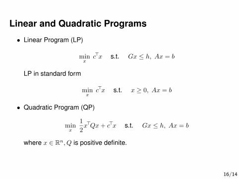
Linear and Quadratic Programs
• Linear Program (LP)
minx
c>x s.t. Gx ≤ h, Ax = b
LP in standard form
minx
c>x s.t. x ≥ 0, Ax = b
• Quadratic Program (QP)
minx
1
2x>Qx+ c>x s.t. Gx ≤ h, Ax = b
where x ∈ Rn, Q is positive definite.
16/14
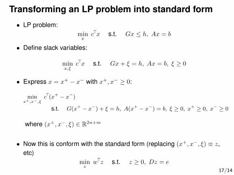
Transforming an LP problem into standard form
• LP problem:minx
c>x s.t. Gx ≤ h, Ax = b
• Define slack variables:
minx,ξ
c>x s.t. Gx+ ξ = h, Ax = b, ξ ≥ 0
• Express x = x+ − x− with x+, x− ≥ 0:
minx+,x−,ξ
c>(x+ − x−)
s.t. G(x+ − x−) + ξ = h, A(x+ − x−) = b, ξ ≥ 0, x+ ≥ 0, x− ≥ 0
where (x+, x−, ξ) ∈ R2n+m
• Now this is conform with the standard form (replacing (x+, x−, ξ) ≡ z,etc)
minz
w>z s.t. z ≥ 0, Dz = e
17/14
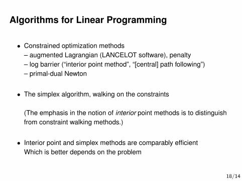
Algorithms for Linear Programming
• Constrained optimization methods– augmented Lagrangian (LANCELOT software), penalty– log barrier (“interior point method”, “[central] path following”)– primal-dual Newton
• The simplex algorithm, walking on the constraints
(The emphasis in the notion of interior point methods is to distinguishfrom constraint walking methods.)
• Interior point and simplex methods are comparably efficientWhich is better depends on the problem
18/14
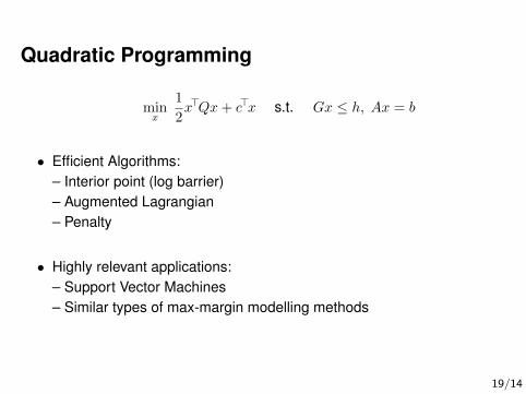
Quadratic Programming
minx
1
2x>Qx+ c>x s.t. Gx ≤ h, Ax = b
• Efficient Algorithms:– Interior point (log barrier)– Augmented Lagrangian– Penalty
• Highly relevant applications:– Support Vector Machines– Similar types of max-margin modelling methods
19/14
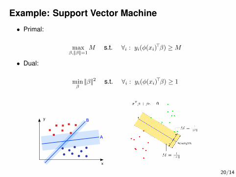
Example: Support Vector Machine
• Primal:
maxβ,||β||=1
M s.t. ∀i : yi(φ(xi)>β) ≥M
• Dual:
minβ||β||2 s.t. ∀i : yi(φ(xi)
>β) ≥ 1
y
x
A
B
20/14