Embed Size (px)
Citation preview
1
© 2004, Ronald J. Williams
Reinforcement Learning and Markov Decision
ProcessesRonald J. Williams
CSG220, Spring 2007
Contains a few slides adapted from two related Andrew Mooretutorials found at http://www.cs.cmu.edu/~awm/tutorials
© 2004, Ronald J. Williams Reinforcement Learning: Slide 2
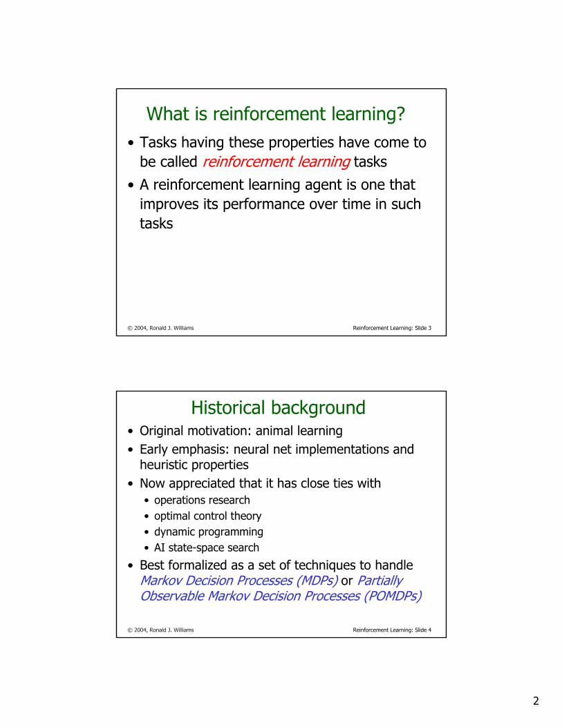
What is reinforcement learning?Key Features:• Agent interacts continually with its environment• Agent has access to performance measure, not
told how it should behave“That was a 3.5”
• Performance measure depends on sequence of actions chosen“Hmm, I wonder where I went wrong ...”• Temporal credit assignment problem
• Not everything known to the agent in advance=> learning required
2
© 2004, Ronald J. Williams Reinforcement Learning: Slide 3
What is reinforcement learning?• Tasks having these properties have come to
be called reinforcement learning tasks
• A reinforcement learning agent is one that improves its performance over time in such tasks
© 2004, Ronald J. Williams Reinforcement Learning: Slide 4
Historical background• Original motivation: animal learning• Early emphasis: neural net implementations and
heuristic properties• Now appreciated that it has close ties with
• operations research• optimal control theory• dynamic programming• AI state-space search
• Best formalized as a set of techniques to handle Markov Decision Processes (MDPs) or Partially Observable Markov Decision Processes (POMDPs)
3
© 2004, Ronald J. Williams Reinforcement Learning: Slide 5
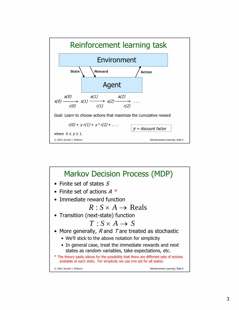
a(0) a(1) a(2)s(0) s(1) s(2) . . .
r(0) r(1) r(2)
Goal: Learn to choose actions that maximize the cumulative reward
r(0) + γ r(1) + γ 2 r(2) + . . .
where 0 ≤ γ ≤ 1.
Reinforcement learning task
Agent
EnvironmentState Reward Action
γ = discount factor
© 2004, Ronald J. Williams Reinforcement Learning: Slide 6
Markov Decision Process (MDP)• Finite set of states S• Finite set of actions A *• Immediate reward function
• Transition (next-state) function
• More generally, R and T are treated as stochastic• We’ll stick to the above notation for simplicity• In general case, treat the immediate rewards and next
states as random variables, take expectations, etc.* The theory easily allows for the possibility that there are different sets of actions
available at each state. For simplicity we use one set for all states.
Reals: →× ASR
SAST →×:
4
© 2004, Ronald J. Williams Reinforcement Learning: Slide 7
Markov Decision Process• If no rewards and only one action, this is
just a Markov chain• Sometimes also called a Controlled Markov
Chain• Overall objective is to determine a policy
such that some measure of cumulative reward is optimized
AS →:π
© 2004, Ronald J. Williams Reinforcement Learning: Slide 8
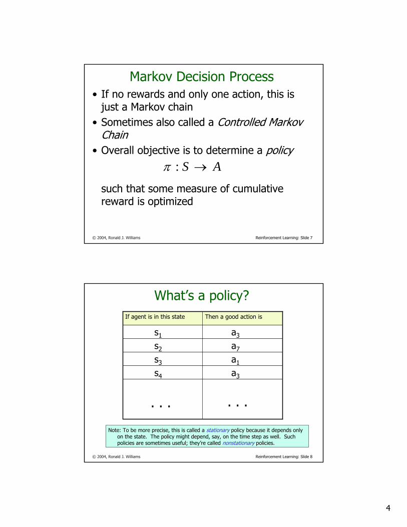
What’s a policy?
a3s4
a1s3
a7s2
a3s1
Then a good action isIf agent is in this state
. . . . . .
Note: To be more precise, this is called a stationary policy because it depends only on the state. The policy might depend, say, on the time step as well. Such policies are sometimes useful; they’re called nonstationary policies.
5
© 2004, Ronald J. Williams Reinforcement Learning: Slide 9
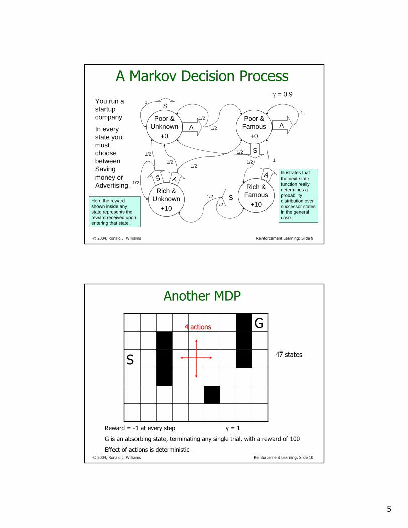
A Markov Decision ProcessYou run a startup company.
In every state you must choose between Saving money or Advertising.
γ = 0.9
Poor &Unknown
+0
Rich &Unknown
+10
Rich &Famous
+10
Poor &Famous
+0
S
AA
S
AA
S
S1
1
1
1/2
1/2
1/2
1/2
1/2
1/2
1/2
1/2
1/2
1/2
Here the reward shown inside any state represents the reward received upon entering that state.
Illustrates that the next-state function really determines a probability distribution over successor states in the general case.
© 2004, Ronald J. Williams Reinforcement Learning: Slide 10
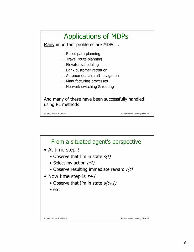
Another MDP
S
G
Reward = -1 at every step γ = 1
G is an absorbing state, terminating any single trial, with a reward of 100
Effect of actions is deterministic
4 actions
47 states
6
© 2004, Ronald J. Williams Reinforcement Learning: Slide 11
Applications of MDPsMany important problems are MDPs….
… Robot path planning… Travel route planning… Elevator scheduling… Bank customer retention… Autonomous aircraft navigation… Manufacturing processes… Network switching & routing
And many of these have been successfully handled using RL methods
© 2004, Ronald J. Williams Reinforcement Learning: Slide 12
From a situated agent’s perspective• At time step t
• Observe that I’m in state s(t)• Select my action a(t)• Observe resulting immediate reward r(t)
• Now time step is t+1• Observe that I’m in state s(t+1)• etc.
7
© 2004, Ronald J. Williams Reinforcement Learning: Slide 13
Value Functions• It turns out that
• RL theory• MDP theory• AI game-tree search
all agree on the idea that evaluating states is a useful thing to do.
• A (state) value function V is any function mapping states to real numbers:
Reals: →SV
© 2004, Ronald J. Williams Reinforcement Learning: Slide 14
A special value function: the return• For any policy , define the return to be the
function assigning to each state the quantity
where• s(0) = s• each action a(t) is chosen according to • each subsequent s(t+1) arises from the transition
function T• each immediate reward r(t) is determined by the
immediate reward function R• is a given discount factor in [0, 1]
π
∑∞
=
=0
)()(t
t trsV γπ Reminder: Use expected values in the stochastic case.
Reals: →SV π
γ
π
8
© 2004, Ronald J. Williams Reinforcement Learning: Slide 15
Technical remarks• If the next state and/or immediate reward
functions are stochastic, then the r(t) values are random variables and the return is defined as the expectation of this sum
• If the MDP has absorbing states, the sum may actually be finite• We stick with this infinite sum notation for the
sake of generality• The discount factor can be taken to be 1 in
absorbing-state MDPs• The formulation we use is called infinite-horizon
© 2004, Ronald J. Williams Reinforcement Learning: Slide 16
Why the discount factor?• Models idea that future rewards are not
worth quite as much the longer into the future they’re received• used in economic models
• Also models situations where there is a nonzero fixed probability 1-γ of termination at any time
• Makes the math work out nicely• with bounded rewards, sum guaranteed to be
finite even in infinite-horizon case
9
© 2004, Ronald J. Williams Reinforcement Learning: Slide 17
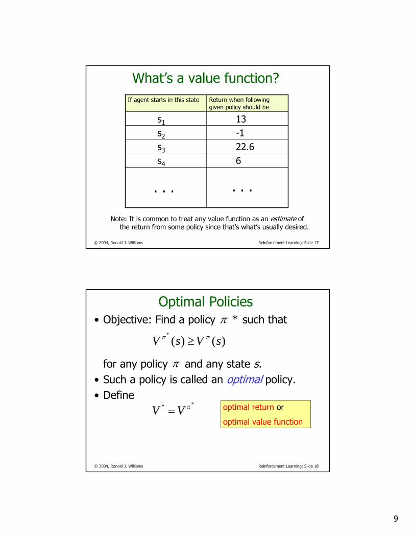
What’s a value function?
6s4
22.6s3
-1s2
13s1
Return when following given policy should be
If agent starts in this state
. . . . . .
Note: It is common to treat any value function as an estimate of the return from some policy since that’s what’s usually desired.
© 2004, Ronald J. Williams Reinforcement Learning: Slide 18
Optimal Policies• Objective: Find a policy such that
for any policy and any state s.• Such a policy is called an optimal policy.• Define
*π
π
)()(*
sVsV ππ ≥
** πVV = optimal return or
optimal value function
10
© 2004, Ronald J. Williams Reinforcement Learning: Slide 19
Interesting factFor every MDP there exists an optimal policy.
It’s a policy such that for every possible start state there is no better option than to follow the policy.
Can you see why this is true?
© 2004, Ronald J. Williams Reinforcement Learning: Slide 20
Finding an Optimal PolicyIdea One:
Run through all possible policies.Select the best.
What’s the problem ??
11
© 2004, Ronald J. Williams Reinforcement Learning: Slide 21
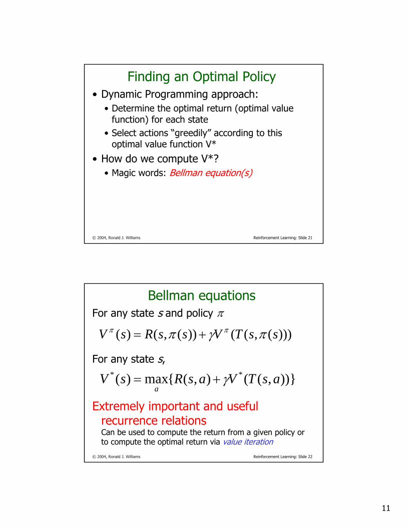
Finding an Optimal Policy• Dynamic Programming approach:
• Determine the optimal return (optimal value function) for each state
• Select actions “greedily” according to this optimal value function V*
• How do we compute V*?• Magic words: Bellman equation(s)
© 2004, Ronald J. Williams Reinforcement Learning: Slide 22
Bellman equationsFor any state s and policy
For any state s,
Extremely important and useful recurrence relationsCan be used to compute the return from a given policy or to compute the optimal return via value iteration
)))(,(())(,()( ssTVssRsV πγπ ππ +=
π
))},((),({max)( ** asTVasRsVa
γ+=
12
© 2004, Ronald J. Williams Reinforcement Learning: Slide 23
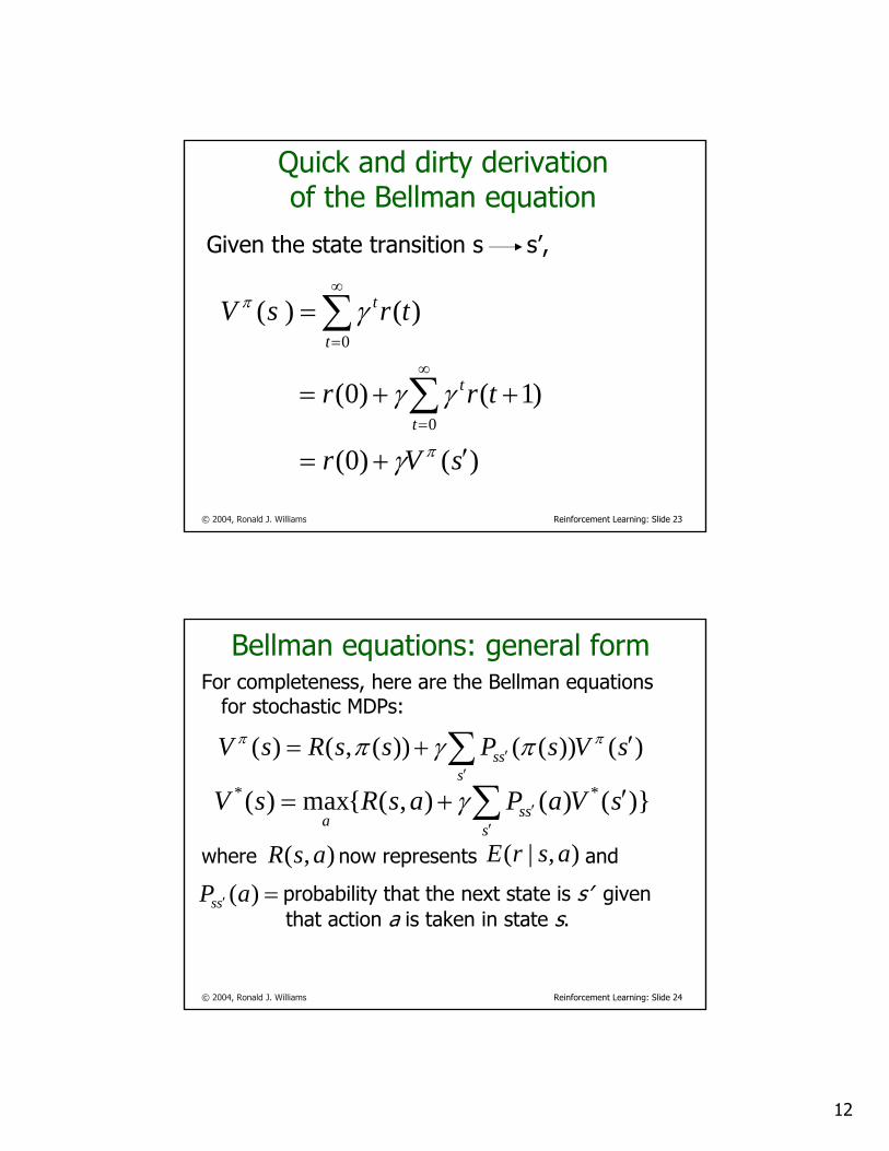
Quick and dirty derivationof the Bellman equation
Given the state transition s s’,
)()0(
)1()0(
)()(
0
0
sVr
trr
trsV
t
t
t
t
′+=
++=
=
∑
∑∞
=
∞
=
π
π
γ
γγ
γ
© 2004, Ronald J. Williams Reinforcement Learning: Slide 24
Bellman equations: general formFor completeness, here are the Bellman equations
for stochastic MDPs:
where now represents and
probability that the next state is s’ given that action a is taken in state s.
)())(())(,()( sVsPssRsVs
ss ′+= ∑′
′ππ πγπ
)}()(),({max)( ** sVaPasRsVs
ssa′+= ∑
′′γ
=′ )(aPss
),( asR ),|( asrE
13
© 2004, Ronald J. Williams Reinforcement Learning: Slide 25
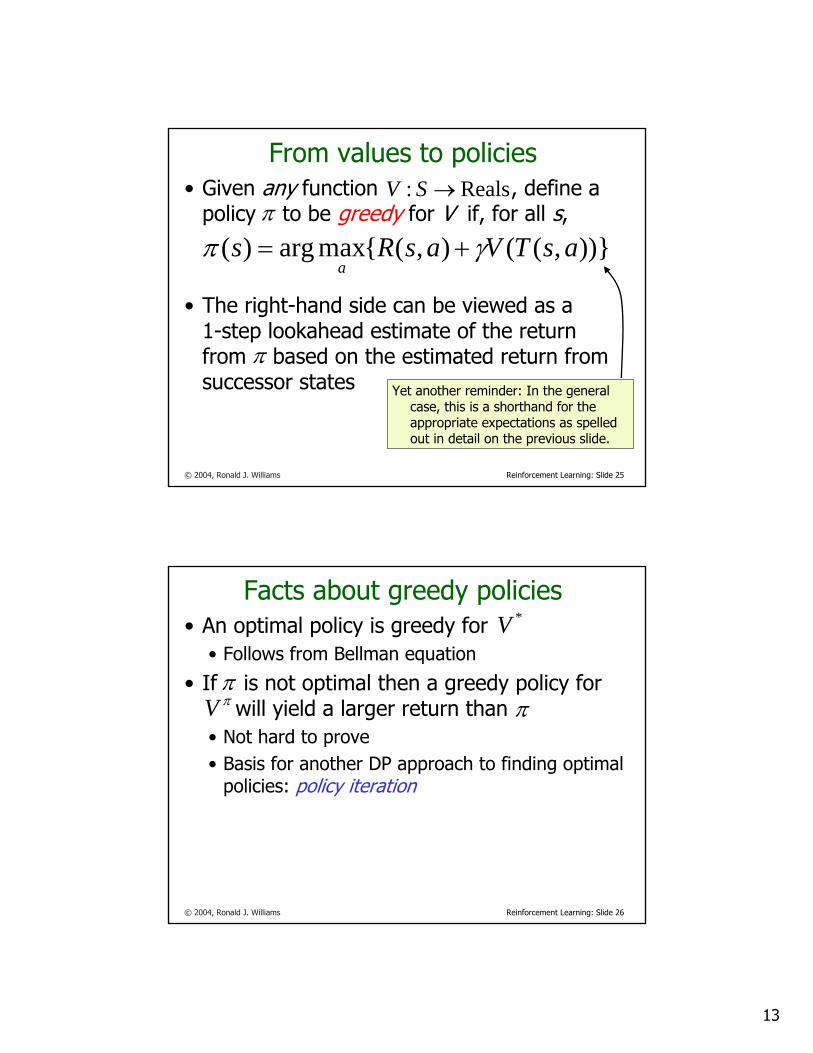
From values to policies• Given any function , define a
policy to be greedy for V if, for all s,
• The right-hand side can be viewed as a1-step lookahead estimate of the return from based on the estimated return from successor states
π))},((),({maxarg)( asTVasRs
aγπ +=
πYet another reminder: In the general
case, this is a shorthand for the appropriate expectations as spelled out in detail on the previous slide.
Reals: →SV
© 2004, Ronald J. Williams Reinforcement Learning: Slide 26
Facts about greedy policies• An optimal policy is greedy for
• Follows from Bellman equation
• If is not optimal then a greedy policy forwill yield a larger return than
• Not hard to prove• Basis for another DP approach to finding optimal
policies: policy iteration
*V
πππV
14
© 2004, Ronald J. Williams Reinforcement Learning: Slide 27
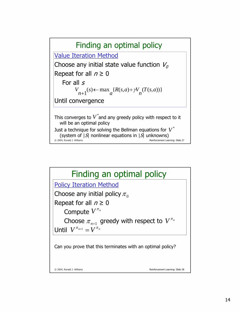
Finding an optimal policyValue Iteration MethodChoose any initial state value function V0
Repeat for all n ≥ 0For all s
Until convergence
This converges to and any greedy policy with respect to it will be an optimal policy
Just a technique for solving the Bellman equations for (system of |S| nonlinear equations in |S| unknowns)
*V
))},((),({max)(1 asTnVasRasnV γ+←+
*V
© 2004, Ronald J. Williams Reinforcement Learning: Slide 28
Finding an optimal policyPolicy Iteration MethodChoose any initial policy Repeat for all n ≥ 0
Compute Choose greedy with respect to
Until
Can you prove that this terminates with an optimal policy?
1+nπ
0π
nV π
nV π
nn VV ππ =+1
15
© 2004, Ronald J. Williams Reinforcement Learning: Slide 29
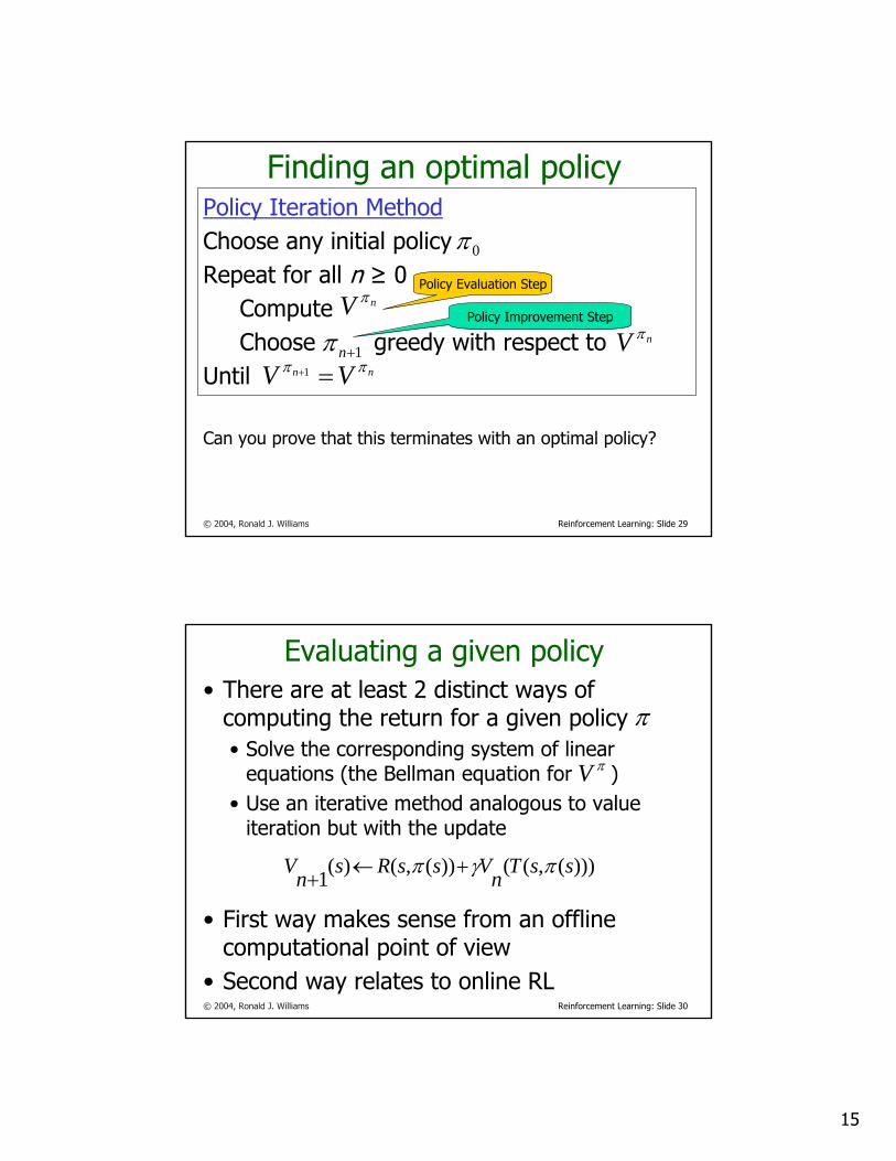
Finding an optimal policyPolicy Iteration MethodChoose any initial policy Repeat for all n ≥ 0
Compute Choose greedy with respect to
Until
Can you prove that this terminates with an optimal policy?
1+nπ
0π
nV π
nV π
nn VV ππ =+1
Policy Evaluation Step
Policy Improvement Step
© 2004, Ronald J. Williams Reinforcement Learning: Slide 30
Evaluating a given policy• There are at least 2 distinct ways of
computing the return for a given policy• Solve the corresponding system of linear
equations (the Bellman equation for )• Use an iterative method analogous to value
iteration but with the update
• First way makes sense from an offline computational point of view
• Second way relates to online RL
π
πV
)))(,(())(,()(1 ssTnVssRsnV πγπ +←+
16
© 2004, Ronald J. Williams Reinforcement Learning: Slide 31
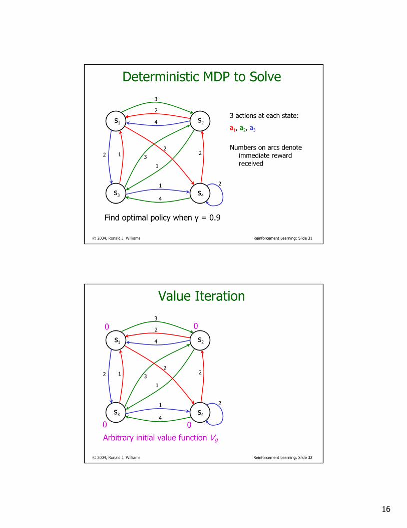
Deterministic MDP to Solve
3 actions at each state:
a1, a2, a3
Numbers on arcs denote immediate reward received
3
2
4
2 1 3
1
2
1
4
2
2
s1 s2
s3 s4
Find optimal policy when γ = 0.9
© 2004, Ronald J. Williams Reinforcement Learning: Slide 32
Value Iteration3
2
4
2 1 3
1
2
1
4
2
2
s1 s2
s3 s4
Arbitrary initial value function V0
0 0
0 0
17
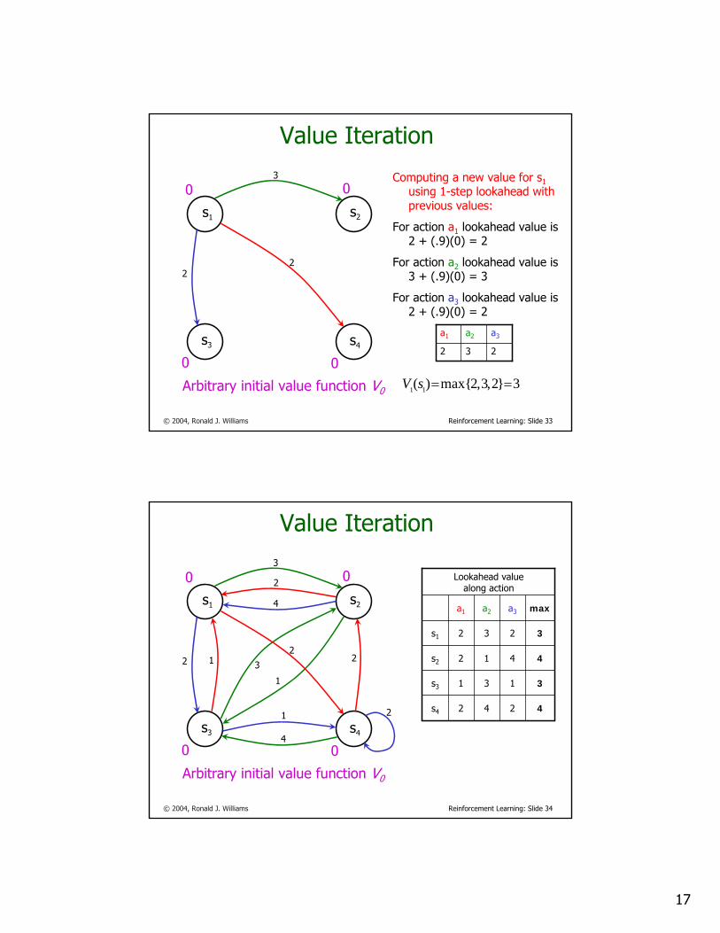
© 2004, Ronald J. Williams Reinforcement Learning: Slide 33
Value Iteration3
22
s1 s2
s3 s4
Arbitrary initial value function V0
0 0
0 0
Computing a new value for s1 using 1-step lookahead with previous values:
For action a1 lookahead value is2 + (.9)(0) = 2
For action a2 lookahead value is3 + (.9)(0) = 3
For action a3 lookahead value is2 + (.9)(0) = 2
3}2,3,2max{)( 11 ==sV
232
a3a2a1
© 2004, Ronald J. Williams Reinforcement Learning: Slide 34
Value Iteration3
2
4
2 1 3
1
2
1
4
2
2
s1 s2
s3 s4
Arbitrary initial value function V0
0 0
0 0
4242s4
3131s3
4412s2
3232s1
maxa3a2a1
Lookahead valuealong action
18
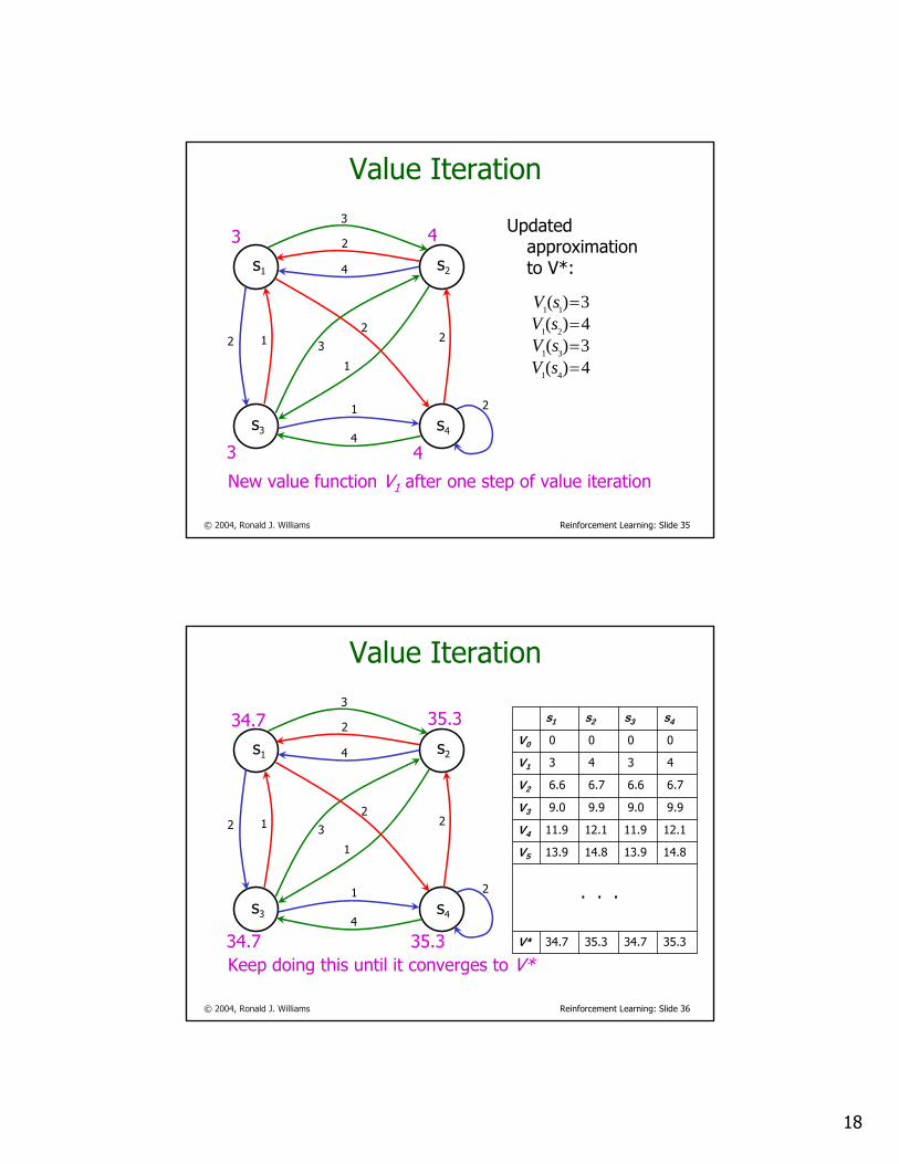
© 2004, Ronald J. Williams Reinforcement Learning: Slide 35
Value Iteration3
2
4
2 1 3
1
2
1
4
2
2
s1 s2
s3 s4
New value function V1 after one step of value iteration
3 4
3 4
4)(3)(4)(3)(
41
31
21
11
====
sVsVsVsV
Updated approximation to V*:
© 2004, Ronald J. Williams Reinforcement Learning: Slide 36
Value Iteration3
2
4
2 1 3
1
2
1
4
2
2
s1 s2
s3 s4
Keep doing this until it converges to V*
34.7 35.3
34.7 35.3
14.813.914.813.9V5
35.334.735.334.7V*
12.111.912.111.9V4
9.99.09.99.0V3
6.76.66.76.6V2
4343V1
0000V0
s4s3s2s1
. . .
19
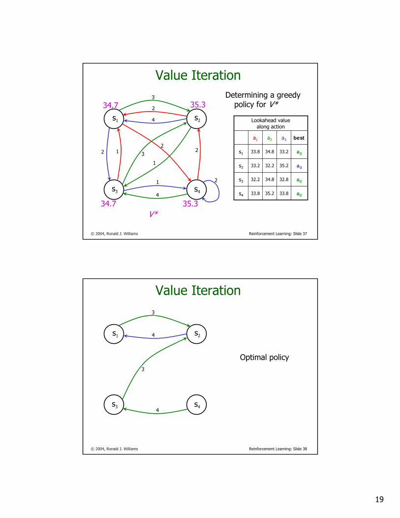
© 2004, Ronald J. Williams Reinforcement Learning: Slide 37
Value Iteration3
2
4
2 1 3
1
2
1
4
2
2
s1 s2
s3 s4
V*
34.7 35.3
34.7 35.3a233.835.233.8s4
a232.834.832.2s3
a335.232.233.2s2
a233.234.833.8s1
besta3a2a1
Lookahead valuealong action
Determining a greedy policy for V*
© 2004, Ronald J. Williams Reinforcement Learning: Slide 38
Value Iteration3
4
3
4
s1 s2
s3 s4
Optimal policy
20
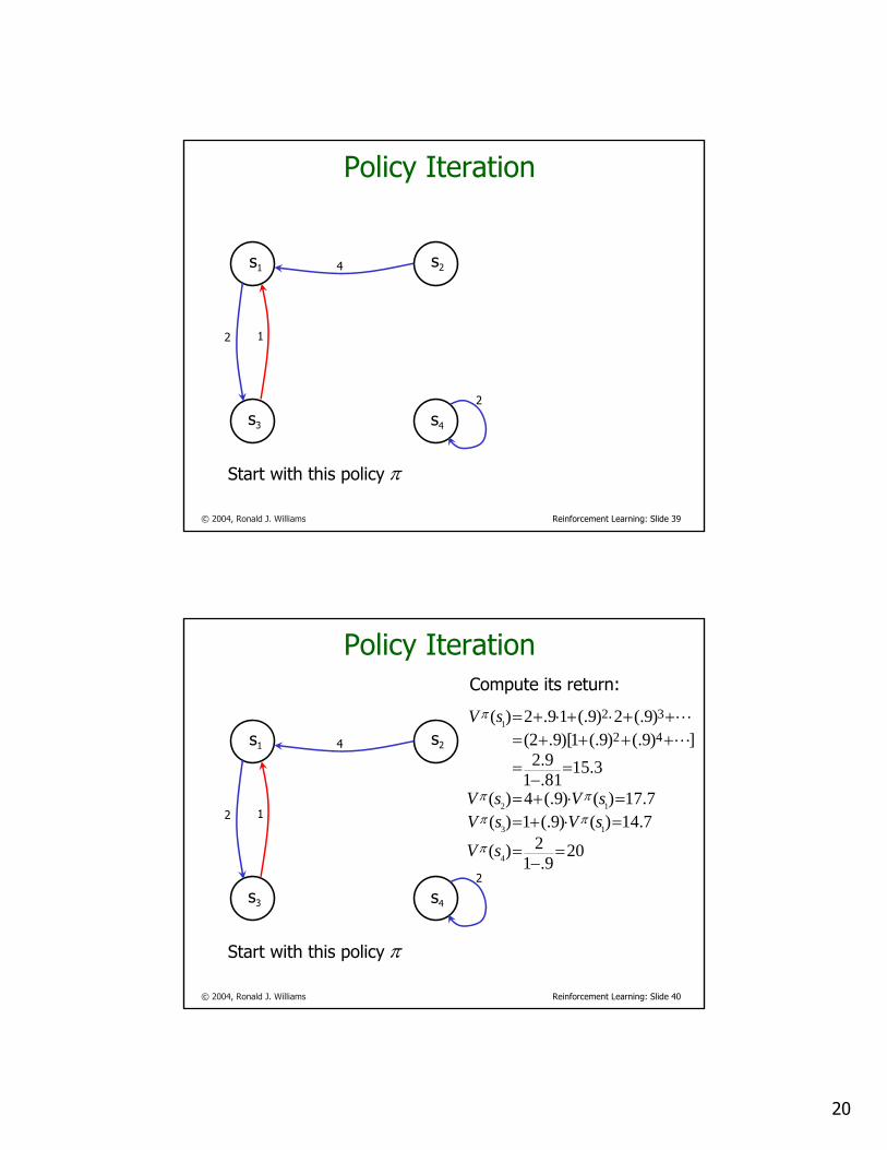
© 2004, Ronald J. Williams Reinforcement Learning: Slide 39
Policy Iteration
4
2 1
2
s1 s2
s3 s4
Start with this policy π
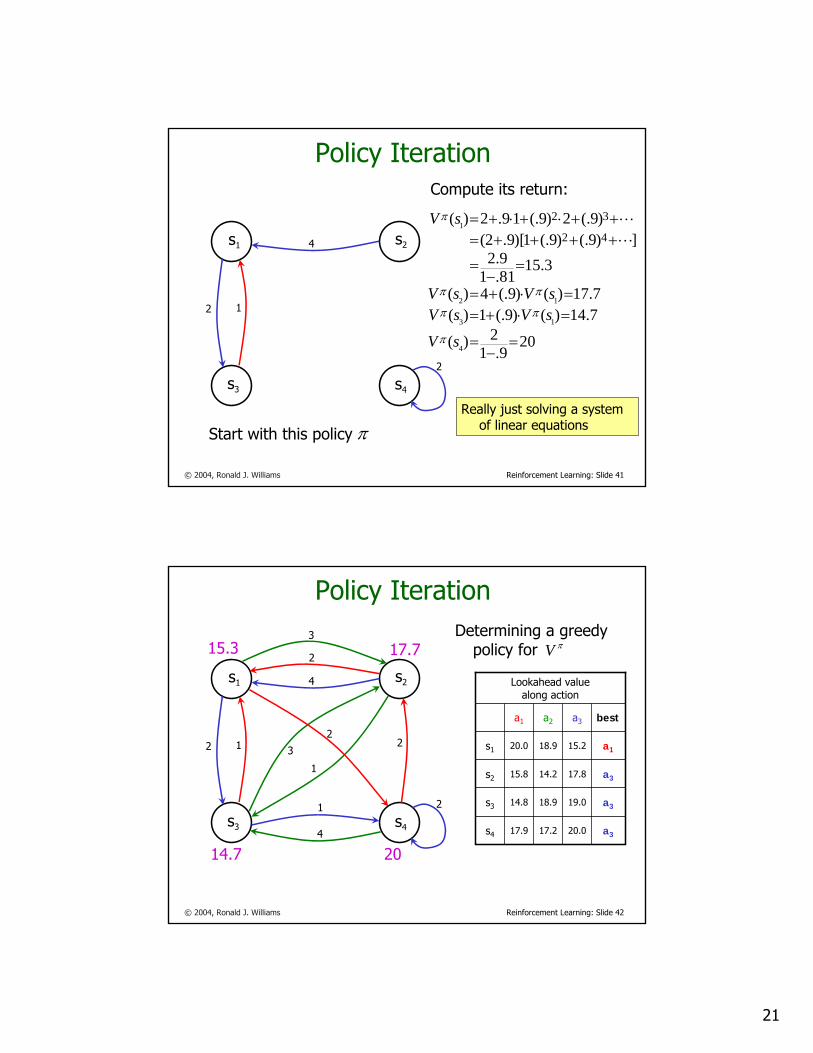
© 2004, Ronald J. Williams Reinforcement Learning: Slide 40
Policy Iteration
4
2 1
2
s1 s2
s3 s4
Start with this policy
209.1
2)(
7.14)()9(.1)(7.17)()9(.4)(
3.1581.19.2
])9(.)9(.1)[9.2()9(.2)9(.19.2)(
4
13
12
1
42
32
=−
=
=⋅+==⋅+=
=−
=
++++=++⋅+⋅+=
sV
sVsVsVsV
sV
π
ππ
ππ
π
L
L
π
Compute its return:
21
© 2004, Ronald J. Williams Reinforcement Learning: Slide 41
Policy Iteration
4
2 1
2
s1 s2
s3 s4
Start with this policy
209.1
2)(
7.14)()9(.1)(7.17)()9(.4)(
3.1581.19.2
])9(.)9(.1)[9.2()9(.2)9(.19.2)(
4
13
12
1
42
32
=−
=
=⋅+==⋅+=
=−
=
++++=++⋅+⋅+=
sV
sVsVsVsV
sV
π
ππ
ππ
π
L
L
πReally just solving a system
of linear equations
Compute its return:
© 2004, Ronald J. Williams Reinforcement Learning: Slide 42
Policy Iteration3
2
4
2 1 3
1
2
1
4
2
2
s1 s2
s3 s4
15.3 17.7
14.7 20
a320.017.217.9s4
a319.018.914.8s3
a317.814.215.8s2
a115.218.920.0s1
besta3a2a1
Lookahead valuealong action
Determining a greedy policy for πV
22
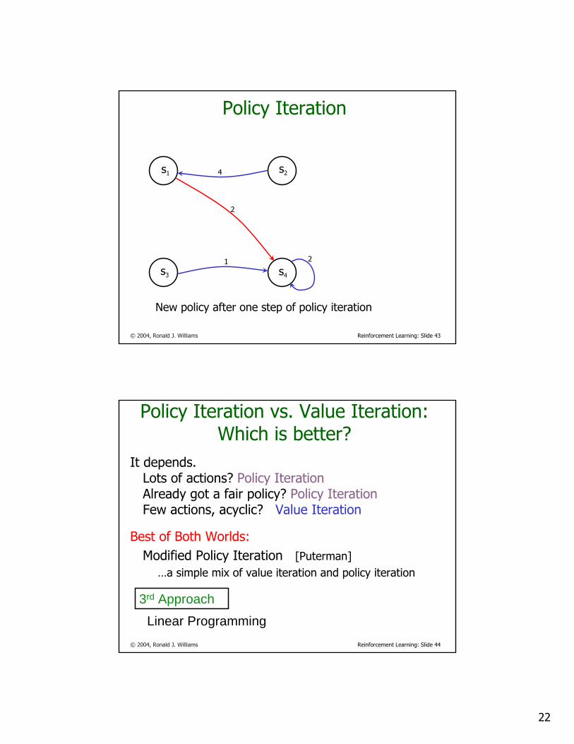
© 2004, Ronald J. Williams Reinforcement Learning: Slide 43
Policy Iteration
4
2
1 2
s1 s2
s3 s4
New policy after one step of policy iteration
© 2004, Ronald J. Williams Reinforcement Learning: Slide 44
Policy Iteration vs. Value Iteration: Which is better?
It depends.Lots of actions? Policy IterationAlready got a fair policy? Policy IterationFew actions, acyclic? Value Iteration
Best of Both Worlds:Modified Policy Iteration [Puterman]
…a simple mix of value iteration and policy iteration
3rd Approach
Linear Programming
23
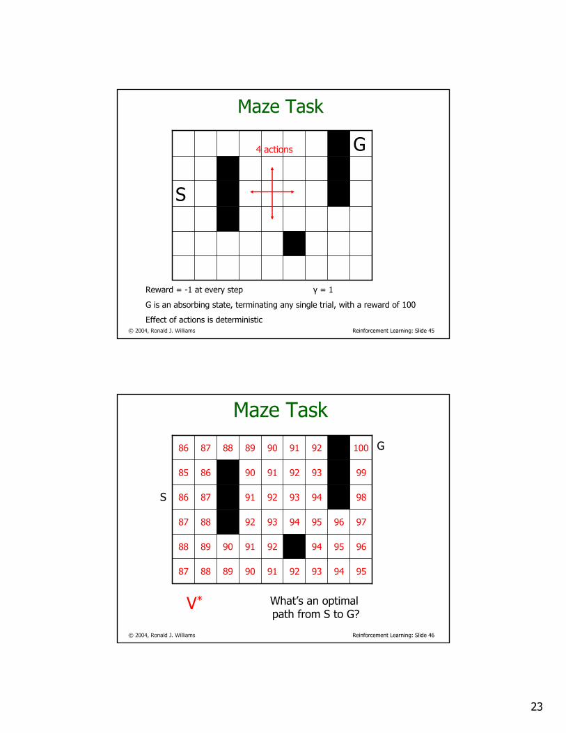
© 2004, Ronald J. Williams Reinforcement Learning: Slide 45
Maze Task
S
G
Reward = -1 at every step γ = 1
G is an absorbing state, terminating any single trial, with a reward of 100
Effect of actions is deterministic
4 actions
© 2004, Ronald J. Williams Reinforcement Learning: Slide 46
Maze Task
959493929190898887
9695949291908988
9796959493928887
989493 92918786
99939291908685
10092919089888786
V* What’s an optimal path from S to G?
S
G
24
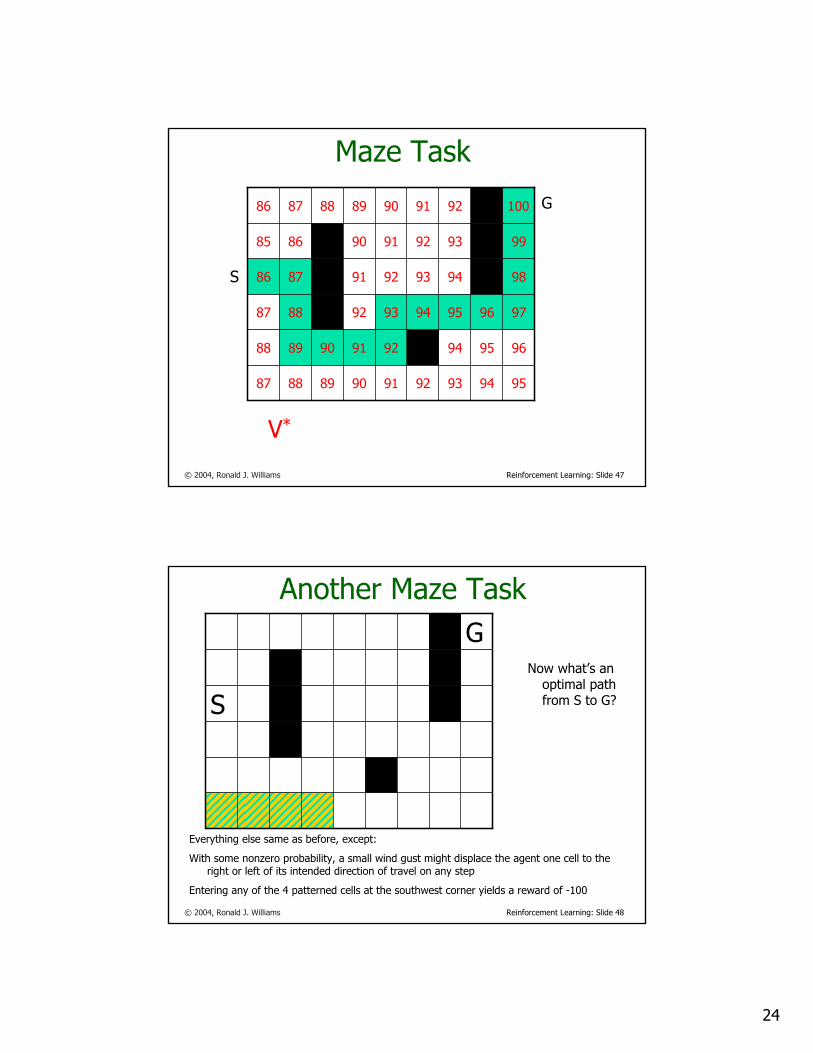
© 2004, Ronald J. Williams Reinforcement Learning: Slide 47
Maze Task
959493929190898887
9695949291908988
9796959493928887
989493 92918786
99939291908685
10092919089888786
V*
S
G
© 2004, Ronald J. Williams Reinforcement Learning: Slide 48
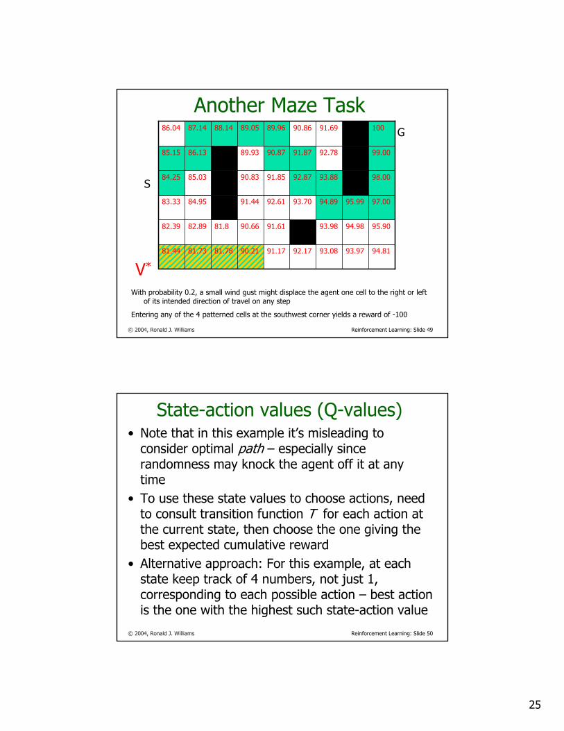
Another Maze Task
S
G
Everything else same as before, except:
With some nonzero probability, a small wind gust might displace the agent one cell to the right or left of its intended direction of travel on any step
Entering any of the 4 patterned cells at the southwest corner yields a reward of -100
Now what’s an optimal path from S to G?
25
© 2004, Ronald J. Williams Reinforcement Learning: Slide 49
Another Maze Task
94.8193.9793.0892.1791.1790.2181.7881.7381.44
95.9094.9893.9891.6190.6681.882.8982.39
97.0095.9994.8993.7092.6191.4484.9583.33
98.0093.8892.8791.8590.8385.0384.25
99.0092.7891.8790.8789.9386.1385.15
10091.6990.8689.9689.0588.1487.1486.04
With probability 0.2, a small wind gust might displace the agent one cell to the right or left of its intended direction of travel on any step
Entering any of the 4 patterned cells at the southwest corner yields a reward of -100
S
G
V*
© 2004, Ronald J. Williams Reinforcement Learning: Slide 50
State-action values (Q-values)• Note that in this example it’s misleading to
consider optimal path – especially since randomness may knock the agent off it at any time
• To use these state values to choose actions, need to consult transition function T for each action at the current state, then choose the one giving the best expected cumulative reward
• Alternative approach: For this example, at each state keep track of 4 numbers, not just 1, corresponding to each possible action – best action is the one with the highest such state-action value
26
© 2004, Ronald J. Williams Reinforcement Learning: Slide 51
Q-Values• For any policy , define
by
where the initial state s(0) = s, the initial actiona(0) = a, and all subsequent states, actions, and rewards arise from the transition, policy, and reward functions, respectively.
• Just like except that action a is taken as the very first step and only after this is policyfollowed
• Bellman equations can be rewritten in terms ofQ-values
π
∑∞
=
=0
)(),(t
t trasQ γπ
Reals: →× ASQπ
πVπ
Once again, the correct expression for a general MDP should use expected values here
© 2004, Ronald J. Williams Reinforcement Learning: Slide 52
Q-Values (cont.)• Define , where is an optimal policy. • There is a corresponding Bellman equation for
since
• Given any state-action value function Q, define a policy to be greedy for Q if
for all s.• An optimal policy is greedy for• Ultimately just a convenient reformulation of the
Bellman equation
** πQQ = *π*Q
),(max)( ** asQsV a=
π),(maxarg)( asQs a=π
*Q
Why it’s convenient will become apparent once we start discussing learning
27
© 2004, Ronald J. Williams Reinforcement Learning: Slide 53
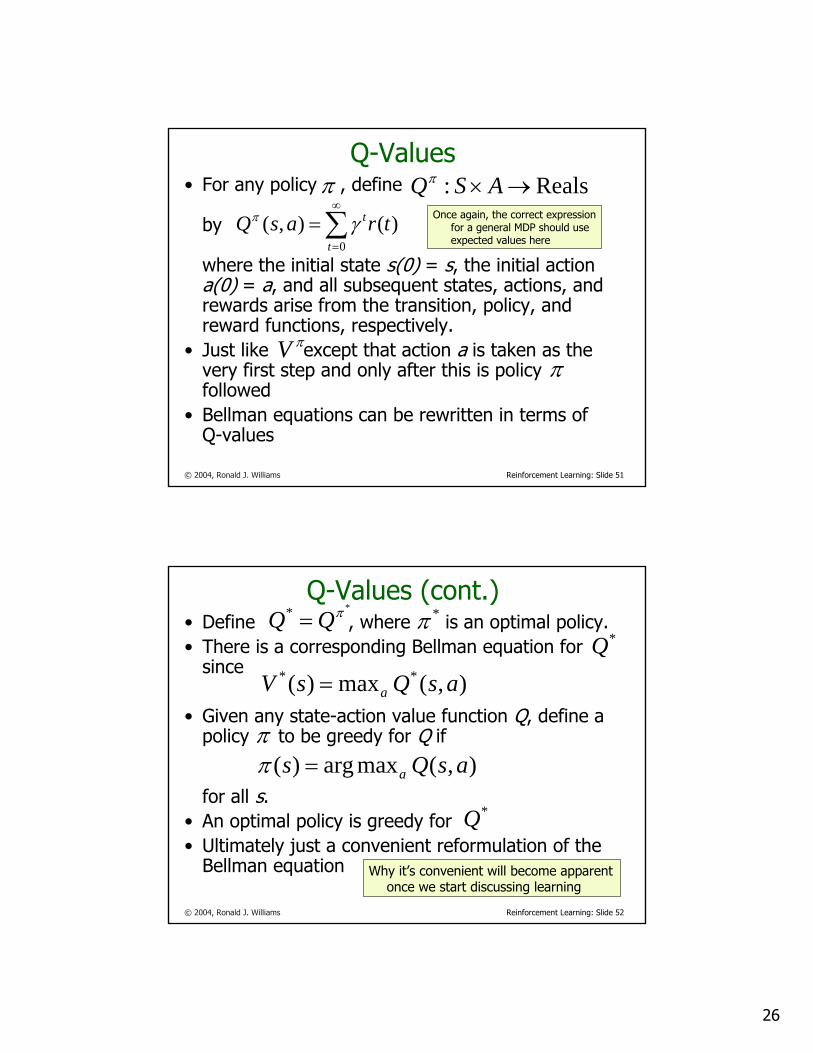
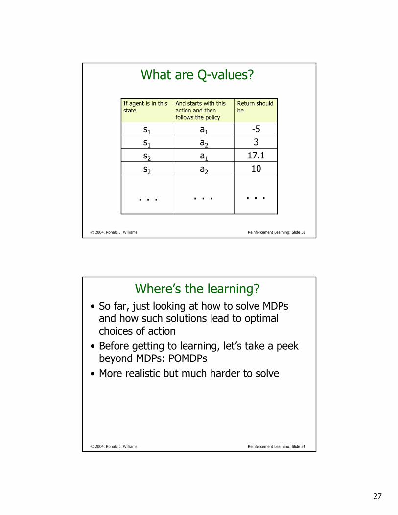
What are Q-values?
10a2s2
17.1a1s2
3a2s1
-5a1s1
Return should be
And starts with this action and then follows the policy
If agent is in this state
. . . . . .. . .
© 2004, Ronald J. Williams Reinforcement Learning: Slide 54
Where’s the learning?• So far, just looking at how to solve MDPs
and how such solutions lead to optimal choices of action
• Before getting to learning, let’s take a peek beyond MDPs: POMDPs
• More realistic but much harder to solve
28
© 2004, Ronald J. Williams Reinforcement Learning: Slide 55
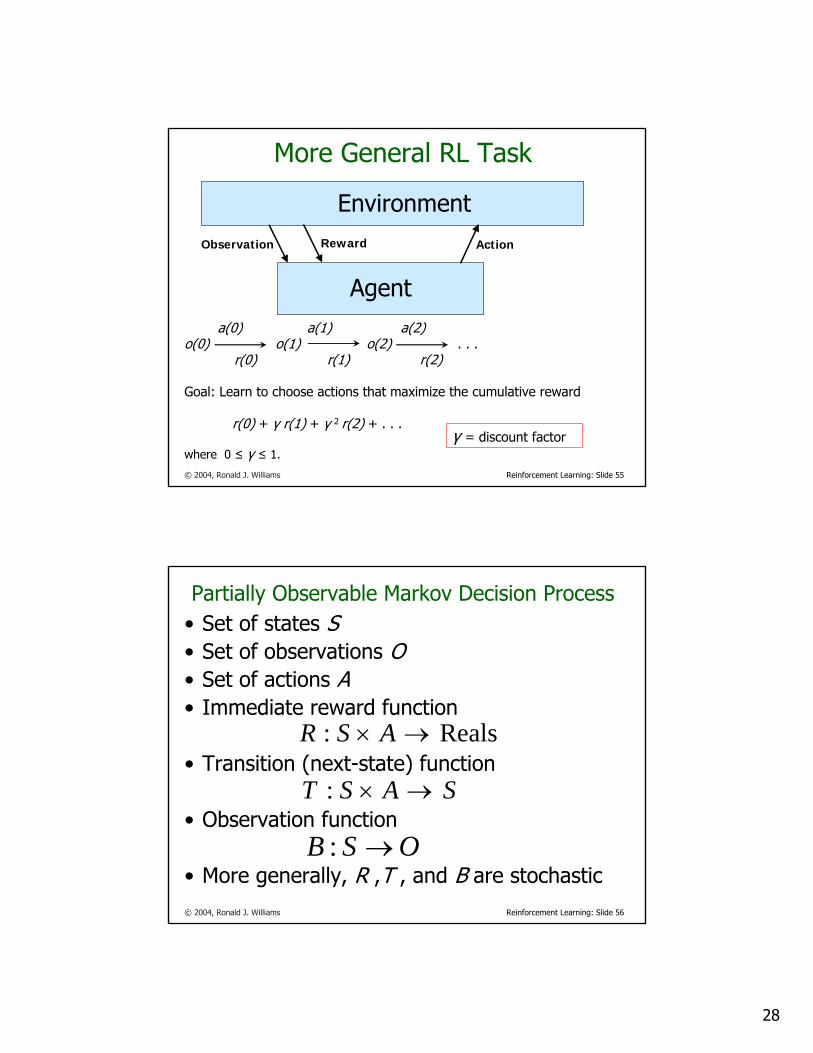
a(0) a(1) a(2)o(0) o(1) o(2) . . .
r(0) r(1) r(2)
Goal: Learn to choose actions that maximize the cumulative reward
r(0) + γ r(1) + γ 2 r(2) + . . .
where 0 ≤ γ ≤ 1.
More General RL Task
γ = discount factor
Agent
EnvironmentObservation Reward Action
© 2004, Ronald J. Williams Reinforcement Learning: Slide 56
Partially Observable Markov Decision Process• Set of states S• Set of observations O• Set of actions A• Immediate reward function
• Transition (next-state) function
• Observation function
• More generally, R ,T , and B are stochastic
Reals: →× ASR
SAST →×:
OSB →:
29
© 2004, Ronald J. Williams Reinforcement Learning: Slide 57
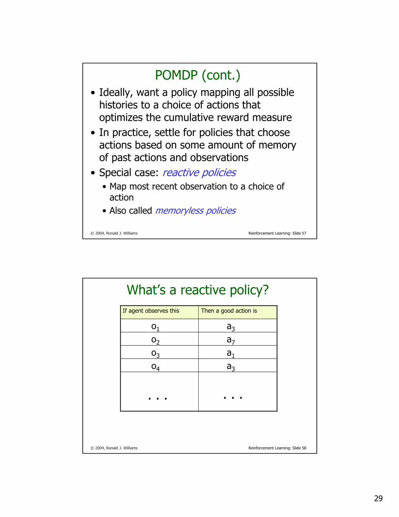
POMDP (cont.)• Ideally, want a policy mapping all possible
histories to a choice of actions that optimizes the cumulative reward measure
• In practice, settle for policies that choose actions based on some amount of memory of past actions and observations
• Special case: reactive policies• Map most recent observation to a choice of
action• Also called memoryless policies
© 2004, Ronald J. Williams Reinforcement Learning: Slide 58
What’s a reactive policy?
a3o4
a1o3
a7o2
a3o1
Then a good action isIf agent observes this
. . . . . .
30
© 2004, Ronald J. Williams Reinforcement Learning: Slide 59
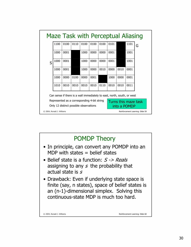
Maze Task with Perceptual Aliasing
001100100010011000100010001000101010
00010000100000010000010000001000
00010010000000100000100000011000
1001000100000000100000011000
1001000100000000100000011000
11010101010001000100011001001100
Can sense if there is a wall immediately to east, north, south, or west
Represented as a corresponding 4-bit string
Only 12 distinct possible observations
G
S
Turns this maze task into a POMDP
© 2004, Ronald J. Williams Reinforcement Learning: Slide 60
POMDP Theory• In principle, can convert any POMDP into an
MDP with states = belief states• Belief state is a function: S -> Reals
assigning to any s the probability that actual state is s
• Drawback: Even if underlying state space is finite (say, n states), space of belief states is an (n-1)-dimensional simplex. Solving this continuous-state MDP is much too hard.
31
© 2004, Ronald J. Williams Reinforcement Learning: Slide 61
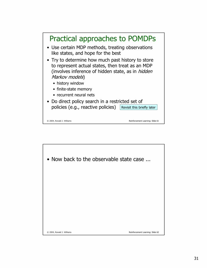
Practical approaches to POMDPs• Use certain MDP methods, treating observations
like states, and hope for the best• Try to determine how much past history to store
to represent actual states, then treat as an MDP (involves inference of hidden state, as in hidden Markov models)• history window• finite-state memory• recurrent neural nets
• Do direct policy search in a restricted set of policies (e.g., reactive policies) Revisit this briefly later
© 2004, Ronald J. Williams Reinforcement Learning: Slide 62
• Now back to the observable state case ...
32
© 2004, Ronald J. Williams Reinforcement Learning: Slide 63
AI state space planning• Traditionally, true world model available a priori• Consider all possible sequences of actions starting
from current state up to some horizon – forms a tree
• Evaluate the states reached at the leaves• Find the best, and choose the first action in that
sequence• How should non-terminal states be evaluated?
• V* would be ideal• But then only 1 step of lookahead would be necessary
• Usual perspective: use depth of search to make up for imperfections in state evaluation
• In control engineering, called receding horizoncontroller
© 2004, Ronald J. Williams Reinforcement Learning: Slide 64
Once again, where’s the learning?• Patience – we’re almost there
33
© 2004, Ronald J. Williams Reinforcement Learning: Slide 65
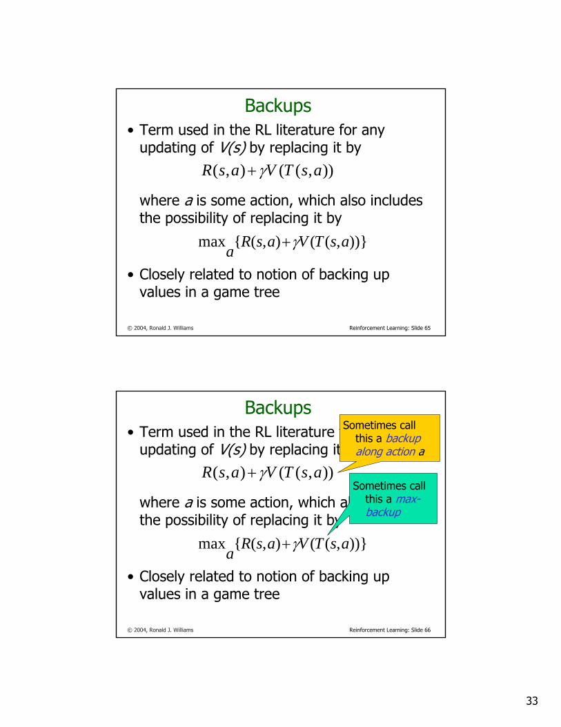
Backups• Term used in the RL literature for any
updating of V(s) by replacing it by
where a is some action, which also includes the possibility of replacing it by
• Closely related to notion of backing up values in a game tree
)),((),( asTVasR γ+
))},((),({max asTVasRa γ+
© 2004, Ronald J. Williams Reinforcement Learning: Slide 66
Backups• Term used in the RL literature for any
updating of V(s) by replacing it by
where a is some action, which also includes the possibility of replacing it by
• Closely related to notion of backing up values in a game tree
)),((),( asTVasR γ+
))},((),({max asTVasRa γ+
Sometimes call this a backupalong action a
Sometimes call this a max-backup
34
© 2004, Ronald J. Williams Reinforcement Learning: Slide 67
Backups• The operation of backing up values is one of
the primary links between MDP theory and RL methods
• Some key facts making these classical MDP algorithms relevant to online learning • value iteration consists solely of (max-)backup
operations• policy evaluation step in policy iteration can be
performed solely with backup operations (along the policy)
• backups modify the value at a state solely based on the values at successor states
© 2004, Ronald J. Williams Reinforcement Learning: Slide 68
Synchronous vs. asynchronous• The value iteration and policy iteration algorithms
demonstrated here use synchronous backups, but asynchronous backups (implementable by “updating in place”) can also be shown to work
• Value iteration and policy iteration can be seen as two ends of a spectrum
• Many ways of interleaving backup steps and policy improvement steps can be shown to work, but not all (Williams & Baird, 1993)
35
© 2004, Ronald J. Williams Reinforcement Learning: Slide 69
Generalized Policy Iteration• GPI coined to apply to the wide range of RL
algorithms that combine simultaneous updating of values and policies in intuitively reasonable ways
• It is known that not every possible GPI algorithm converges to an optimal policy
• However, only known counterexamples are contrived
• Remains an open question whether some of the ones found successful in practice are mathematically guaranteed to work
© 2004, Ronald J. Williams Reinforcement Learning: Slide 70
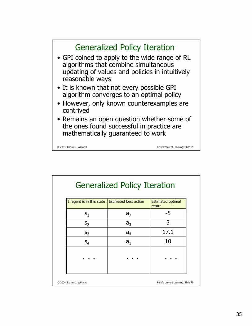
Generalized Policy Iteration
10a1s4
17.1a4s3
3a3s2
-5a7s1
Estimated optimal return
Estimated best actionIf agent is in this state
. . . . . .. . .
36
© 2004, Ronald J. Williams Reinforcement Learning: Slide 71
Learning – Finally!• Almost everything we’ve discussed so far is
“classical” MDP (or POMDP) theory• Transition, reward functions known a priori• Issue is purely one of (off-line) planning
• Four ways RL theory goes beyond this• Assume transition and/or reward functions not known a
priori – must be discovered through environmental interactions
• Try to address tasks for which classical approach is intractable
• Take seriously the idea that policy and/or values not represented simply using table lookup
• Even when T and R are known, only do a kind of online planning in parts of state space actually experienced
© 2004, Ronald J. Williams Reinforcement Learning: Slide 72
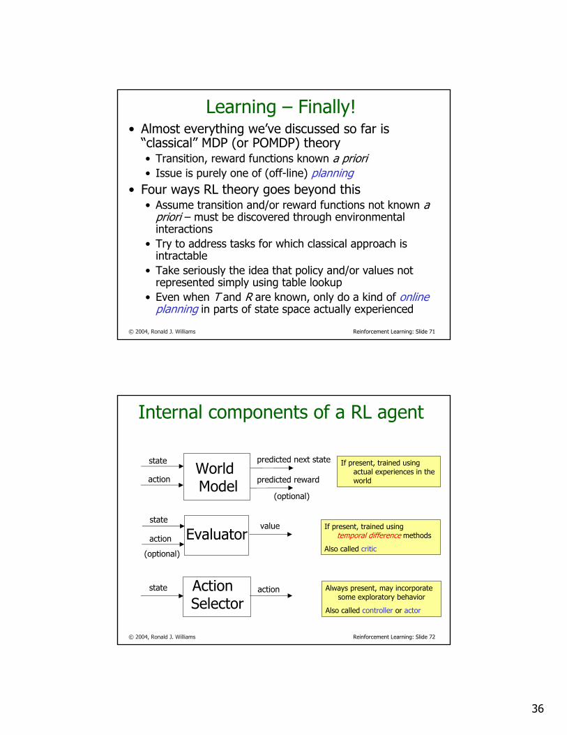
Internal components of a RL agent
Action Selector
state action
Evaluatorstate
action
(optional)
value
If present, trained using actual experiences in the world
WorldModel
state
action
predicted next state
predicted reward
(optional)
If present, trained usingtemporal difference methods
Also called critic
Always present, may incorporate some exploratory behavior
Also called controller or actor
37
© 2004, Ronald J. Williams Reinforcement Learning: Slide 73
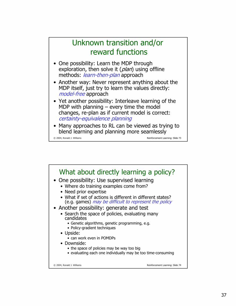
Unknown transition and/orreward functions
• One possibility: Learn the MDP through exploration, then solve it (plan) using offline methods: learn-then-plan approach
• Another way: Never represent anything about the MDP itself, just try to learn the values directly: model-free approach
• Yet another possibility: Interleave learning of the MDP with planning – every time the model changes, re-plan as if current model is correct: certainty-equivalence planning
• Many approaches to RL can be viewed as trying to blend learning and planning more seamlessly
© 2004, Ronald J. Williams Reinforcement Learning: Slide 74
What about directly learning a policy?• One possibility: Use supervised learning
• Where do training examples come from?• Need prior expertise• What if set of actions is different in different states?
(e.g. games) may be difficult to represent the policy• Another possibility: generate and test
• Search the space of policies, evaluating many candidates
• Genetic algorithms, genetic programming, e.g.• Policy-gradient techniques
• Upside:• can work even in POMDPs
• Downside:• the space of policies may be way too big• evaluating each one individually may be too time-consuming
38
© 2004, Ronald J. Williams Reinforcement Learning: Slide 75
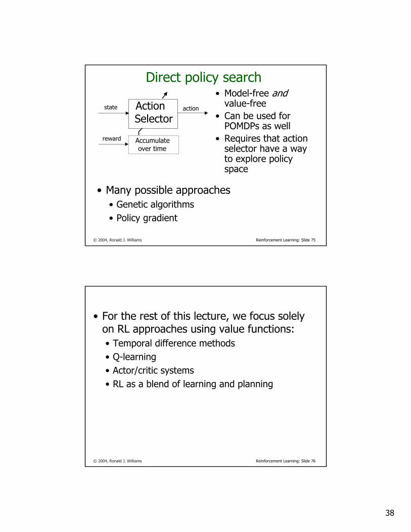
Direct policy search• Model-free and
value-free• Can be used for
POMDPs as well• Requires that action
selector have a way to explore policy space
Action Selector
state action
Accumulate over time
reward
• Many possible approaches• Genetic algorithms• Policy gradient
© 2004, Ronald J. Williams Reinforcement Learning: Slide 76
• For the rest of this lecture, we focus solely on RL approaches using value functions:• Temporal difference methods• Q-learning• Actor/critic systems• RL as a blend of learning and planning
39
© 2004, Ronald J. Williams Reinforcement Learning: Slide 77
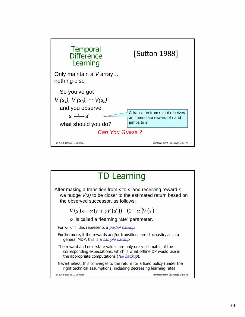
Temporal Difference Learning
Only maintain a V array…nothing else
So you’ve gotV (s1), V (s2), ··· V(sn)
and you observes r s’
what should you do?Can You Guess ?
[Sutton 1988]
A transition from s that receives an immediate reward of r and jumps to s’
© 2004, Ronald J. Williams Reinforcement Learning: Slide 78
TD LearningAfter making a transition from s to s’ and receiving reward r,
we nudge V(s) to be closer to the estimated return based on the observed successor, as follows:
( ) ( )( ) ( ) ( )
s1ssα
αγα VVrV −+′+←is called a “learning rate” parameter.
For this represents a partial backup.
Furthermore, if the rewards and/or transitions are stochastic, as in a general MDP, this is a sample backup.
The reward and next-state values are only noisy estimates of the corresponding expectations, which is what offline DP would use in the appropriate computations (full backup).
Nevertheless, this converges to the return for a fixed policy (under the right technical assumptions, including decreasing learning rate)
1 <α
40
© 2004, Ronald J. Williams Reinforcement Learning: Slide 79
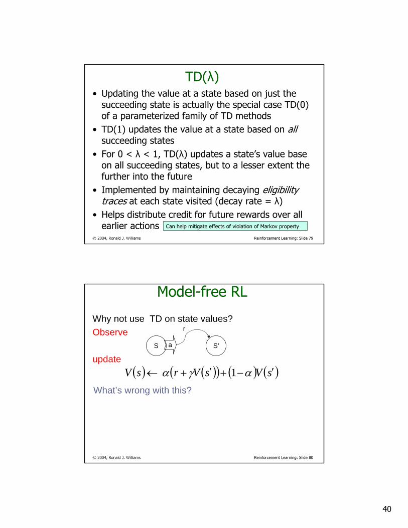
TD(λ)• Updating the value at a state based on just the
succeeding state is actually the special case TD(0) of a parameterized family of TD methods
• TD(1) updates the value at a state based on allsucceeding states
• For 0 < λ < 1, TD(λ) updates a state’s value base on all succeeding states, but to a lesser extent the further into the future
• Implemented by maintaining decaying eligibility traces at each state visited (decay rate = λ)
• Helps distribute credit for future rewards over all earlier actions Can help mitigate effects of violation of Markov property
© 2004, Ronald J. Williams Reinforcement Learning: Slide 80
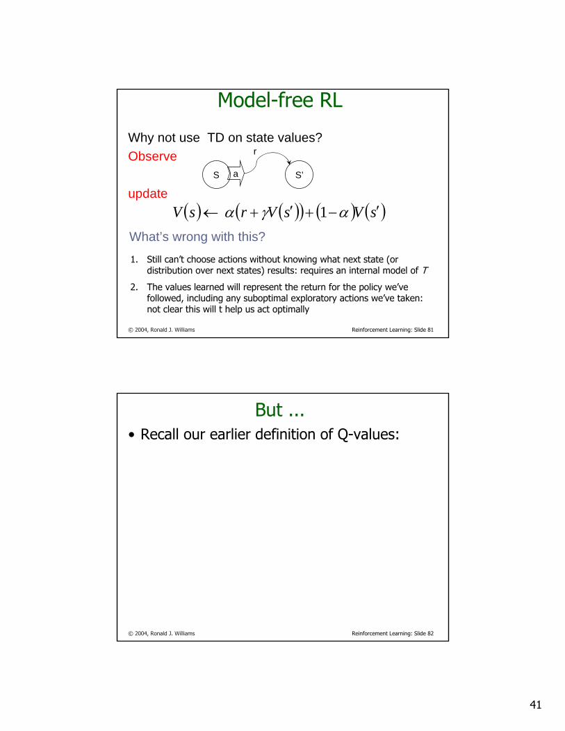
Model-free RL
Why not use TD on state values?Observe
updateS a S’
r
( ) ( )( ) ( ) ( )sVsVrsV ′−+′+← αγα 1 What’s wrong with this?
41
© 2004, Ronald J. Williams Reinforcement Learning: Slide 81
Model-free RL
Why not use TD on state values?Observe
updateS a S’
r
( ) ( )( ) ( ) ( )sVsVrsV ′−+′+← αγα 1 What’s wrong with this?
1. Still can’t choose actions without knowing what next state (or distribution over next states) results: requires an internal model of T
2. The values learned will represent the return for the policy we’ve followed, including any suboptimal exploratory actions we’ve taken: not clear this will t help us act optimally
© 2004, Ronald J. Williams Reinforcement Learning: Slide 82
But ...• Recall our earlier definition of Q-values:
42
© 2004, Ronald J. Williams Reinforcement Learning: Slide 83
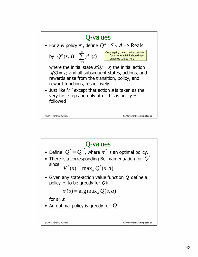
Q-values• For any policy , define
by
where the initial state s(0) = s, the initial actiona(0) = a, and all subsequent states, actions, and rewards arise from the transition, policy, and reward functions, respectively.
• Just like except that action a is taken as the very first step and only after this is policyfollowed
π
∑∞
=
=0
)(),(t
t trasQ γπ
Reals: →× ASQπ
πVπ
Once again, the correct expression for a general MDP should use expected values here
© 2004, Ronald J. Williams Reinforcement Learning: Slide 84
Q-values• Define , where is an optimal policy. • There is a corresponding Bellman equation for
since
• Given any state-action value function Q, define a policy to be greedy for Q if
for all s.• An optimal policy is greedy for
** πQQ = *π*Q
),(max)( ** asQsV a=
π),(maxarg)( asQs a=π
*Q
43
© 2004, Ronald J. Williams Reinforcement Learning: Slide 85
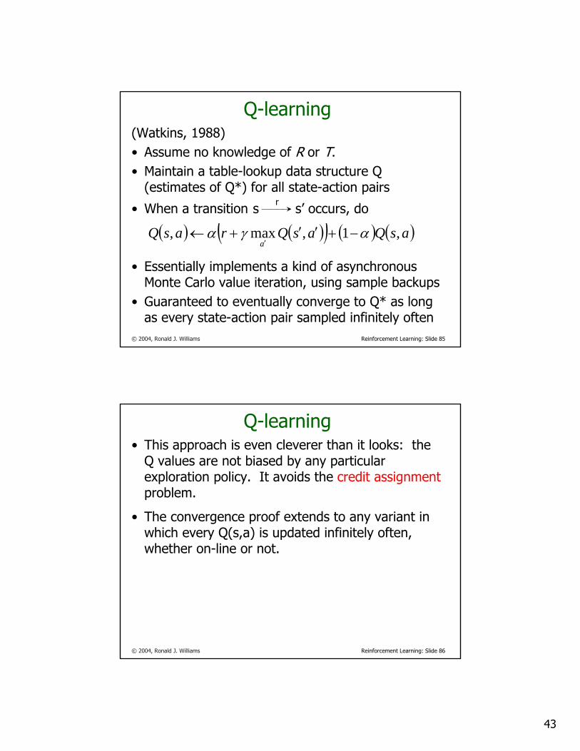
Q-learning(Watkins, 1988)• Assume no knowledge of R or T.• Maintain a table-lookup data structure Q
(estimates of Q*) for all state-action pairs
• When a transition s r s’ occurs, do
• Essentially implements a kind of asynchronous Monte Carlo value iteration, using sample backups
• Guaranteed to eventually converge to Q* as long as every state-action pair sampled infinitely often
( ) ( )( ) ( ) ( )asQasQrasQa
,1,max, αγα −+′′+←′
© 2004, Ronald J. Williams Reinforcement Learning: Slide 86
Q-learning• This approach is even cleverer than it looks: the
Q values are not biased by any particular exploration policy. It avoids the credit assignmentproblem.
• The convergence proof extends to any variant in which every Q(s,a) is updated infinitely often, whether on-line or not.
44
© 2004, Ronald J. Williams Reinforcement Learning: Slide 87
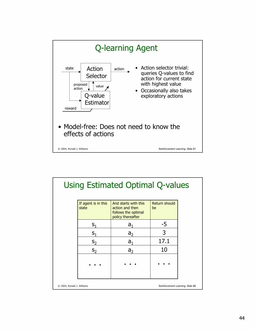
Q-learning Agent
• Action selector trivial: queries Q-values to find action for current state with highest value
• Occasionally also takes exploratory actions
• Model-free: Does not need to know the effects of actions
Q-value Estimator
Action Selector
state action
proposed action
value
reward
© 2004, Ronald J. Williams Reinforcement Learning: Slide 88
Using Estimated Optimal Q-values
10a2s2
17.1a1s2
3a2s1
-5a1s1
Return should be
And starts with this action and then follows the optimal policy thereafter
If agent is in this state
. . . . . .. . .
45
© 2004, Ronald J. Williams Reinforcement Learning: Slide 89
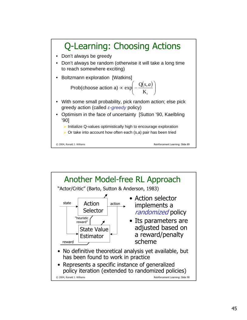
Q-Learning: Choosing Actions• Don’t always be greedy• Don’t always be random (otherwise it will take a long time
to reach somewhere exciting)
• Boltzmann exploration [Watkins]
Prob(choose action a)
• With some small probability, pick random action; else pick greedy action (called ε-greedy policy)
• Optimism in the face of uncertainty [Sutton ’90, Kaelbling ’90]
Initialize Q-values optimistically high to encourage explorationOr take into account how often each (s,a) pair has been tried
( )⎟⎟⎠
⎞⎜⎜⎝
⎛−∝
t
asK
,Qexp
© 2004, Ronald J. Williams Reinforcement Learning: Slide 90
Another Model-free RL Approach
• Action selector implements a randomized policy
• Its parameters are adjusted based on a reward/penalty scheme
• No definitive theoretical analysis yet available, but has been found to work in practice
• Represents a specific instance of generalized policy iteration (extended to randomized policies)
State Value Estimator
Action Selector
state action
“heuristic reward”
reward
“Actor/Critic” (Barto, Sutton & Anderson, 1983)
46
© 2004, Ronald J. Williams Reinforcement Learning: Slide 91
Learning or planning?• Classical DP emphasis for optimal control
• Dynamics and reward structure known• Off-line computation
• Traditional RL emphasis• Dynamics and/or reward structure initially
unknown• On-line learning
• Computation of an optimal policy off-line with known dynamics and reward structure can be regarded as planning
© 2004, Ronald J. Williams Reinforcement Learning: Slide 92
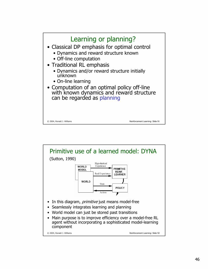
Primitive use of a learned model: DYNA
• In this diagram, primitive just means model-free • Seamlessly integrates learning and planning• World model can just be stored past transitions• Main purpose is to improve efficiency over a model-free RL
agent without incorporating a sophisticated model-learning component
(Sutton, 1990)
47
© 2004, Ronald J. Williams Reinforcement Learning: Slide 93
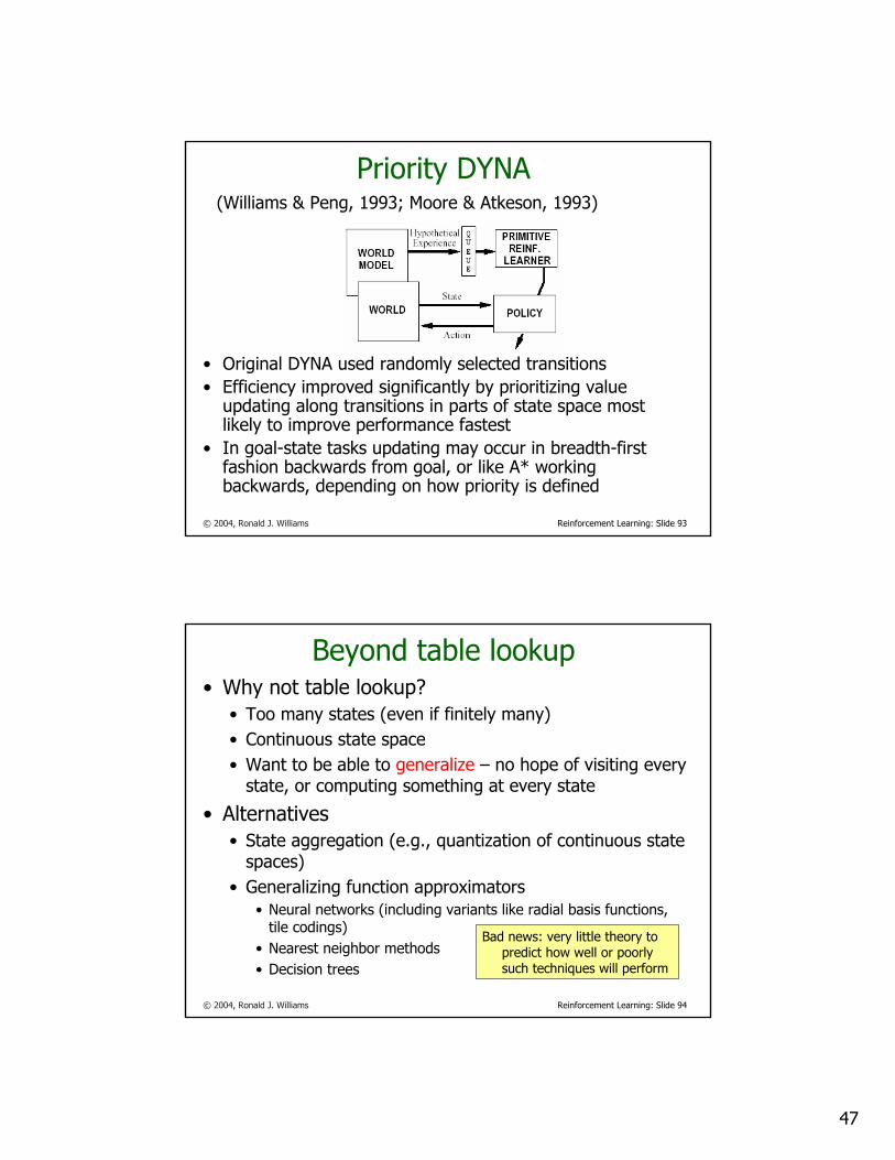
Priority DYNA
• Original DYNA used randomly selected transitions• Efficiency improved significantly by prioritizing value
updating along transitions in parts of state space most likely to improve performance fastest
• In goal-state tasks updating may occur in breadth-first fashion backwards from goal, or like A* working backwards, depending on how priority is defined
(Williams & Peng, 1993; Moore & Atkeson, 1993)
© 2004, Ronald J. Williams Reinforcement Learning: Slide 94
Beyond table lookup• Why not table lookup?
• Too many states (even if finitely many)• Continuous state space• Want to be able to generalize – no hope of visiting every
state, or computing something at every state
• Alternatives• State aggregation (e.g., quantization of continuous state
spaces)• Generalizing function approximators
• Neural networks (including variants like radial basis functions,tile codings)
• Nearest neighbor methods• Decision trees
Bad news: very little theory to predict how well or poorly such techniques will perform

48
© 2004, Ronald J. Williams Reinforcement Learning: Slide 95
Challenges• How do we apply these techniques to infinite (e.g.,
continuous), or even just very large, state spaces?• Pole-balancer• Truck backer-upper• Mountain car (or puck-on-a-hill)• Bioreactor• Acrobot• Multi-jointed snake• Continuous mazes
• Two basic approaches for continuous state spaces• Quantize (to obtain a finite-state approximation)
• One promising approach: adaptive partitioning• Use function approximators (nearest-neighbor, neural
networks, radial basis functions, tile codings, etc.)
Together with finite-state mazes of various kinds, these tasks have become benchmark test problems for RL techniques
© 2004, Ronald J. Williams Reinforcement Learning: Slide 96
Pole balancer

49
© 2004, Ronald J. Williams Reinforcement Learning: Slide 97
Truck backer-upper
© 2004, Ronald J. Williams Reinforcement Learning: Slide 98
Puck on a hill (or “mountain car”)

50
© 2004, Ronald J. Williams Reinforcement Learning: Slide 99
Bioreactor
inflow rate = w contains nutrients
outflow rate = w
contains cells c1 and nutrients c2
© 2004, Ronald J. Williams Reinforcement Learning: Slide 100
Acrobot
51
© 2004, Ronald J. Williams Reinforcement Learning: Slide 101
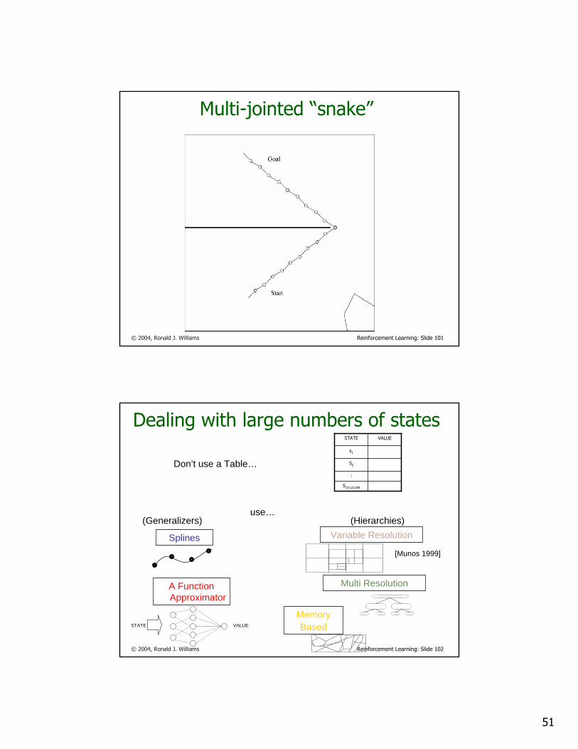
Multi-jointed “snake”
© 2004, Ronald J. Williams Reinforcement Learning: Slide 102
Dealing with large numbers of states
S15122189
:
S2
s1
VALUESTATE
Don’t use a Table…
use…(Generalizers) (Hierarchies)
Splines
A Function Approximator
Variable Resolution
Multi Resolution
MemoryBasedSTATE VALUE
[Munos 1999]
52
© 2004, Ronald J. Williams Reinforcement Learning: Slide 103
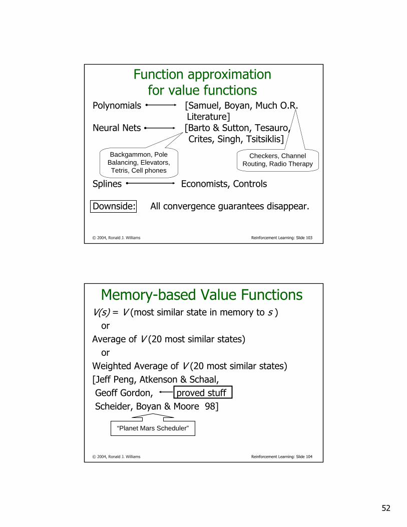
Function approximationfor value functions
Polynomials [Samuel, Boyan, Much O.R.Literature]
Neural Nets [Barto & Sutton, Tesauro, Crites, Singh, Tsitsiklis]
Splines Economists, Controls
Downside: All convergence guarantees disappear.
Backgammon, Pole Balancing, Elevators, Tetris, Cell phones
Checkers, Channel Routing, Radio Therapy
© 2004, Ronald J. Williams Reinforcement Learning: Slide 104
Memory-based Value FunctionsV(s) = V (most similar state in memory to s )
orAverage of V (20 most similar states)
orWeighted Average of V (20 most similar states)[Jeff Peng, Atkenson & Schaal,Geoff Gordon, proved stuffScheider, Boyan & Moore 98]
“Planet Mars Scheduler”
53
© 2004, Ronald J. Williams Reinforcement Learning: Slide 105
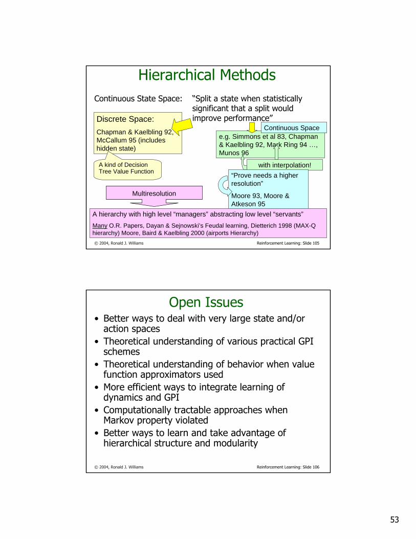
Hierarchical MethodsContinuous State Space: “Split a state when statistically
significant that a split would improve performance”
e.g. Simmons et al 83, Chapman & Kaelbling 92, Mark Ring 94 …, Munos 96
with interpolation!“Prove needs a higher resolution”
Moore 93, Moore & Atkeson 95
Discrete Space:Chapman & Kaelbling 92, McCallum 95 (includes hidden state)
A kind of Decision Tree Value Function
Multiresolution
A hierarchy with high level “managers” abstracting low level “servants”Many O.R. Papers, Dayan & Sejnowski’s Feudal learning, Dietterich 1998 (MAX-Q hierarchy) Moore, Baird & Kaelbling 2000 (airports Hierarchy)
Continuous Space
© 2004, Ronald J. Williams Reinforcement Learning: Slide 106
Open Issues• Better ways to deal with very large state and/or
action spaces• Theoretical understanding of various practical GPI
schemes• Theoretical understanding of behavior when value
function approximators used• More efficient ways to integrate learning of
dynamics and GPI• Computationally tractable approaches when
Markov property violated• Better ways to learn and take advantage of
hierarchical structure and modularity
54
© 2004, Ronald J. Williams Reinforcement Learning: Slide 107
Valuable References• Books
• Bertsekas, D. P. & Tsitsiklis, J. N. (1996). Neuro-Dynamic Programming. Belmont, MA: Athena Scientific
• Sutton, R. S. & Barto, A. G. (1998). Reinforcement Learning: An Introduction. Cambridge, MA: MIT Press
• Survey paper• Kaelbling, L. P., Littman, M. & Moore, A. (1996).
“Reinforcement learning: a survey,” Journal of Artificial Intelligence Research, Vol. 4, pp. 237-285. (Available as a link off the main Andrew Moore tutorials web page.)
© 2004, Ronald J. Williams Reinforcement Learning: Slide 108
What You Should Know• Definition of an MDP (and a POMDP)• How to solve an MDP
• using value iteration• using policy iteration
• Model-free learning (TD) for predicting delayed rewards
• How to formulate RL tasks as MDPs (or POMDPs)
• Q-learning (including being able to work through small simulated examples of RL)