CSE599i: Online and Adaptive Machine Learning Winter 2018 ...Lecture 17: Reinforcement Learning, Finite Markov Decision Processes 2 De nition 1. (Finite Markov decision processes)

CSE599i: Online and Adaptive Machine Learning Winter 2018

Lecture 17: Reinforcement Learning, Finite Markov Decision ProcessesLecturer: Kevin Jamieson Scribes: Aida Amini, Kousuke Ariga, James Ferguson, Yujia Wu

Disclaimer: These notes have not been subjected to the usual scrutiny reserved for formal publications.They may be distributed outside this class only with the permission of the Instructor.

1 Finite Markov decision processes

Finite Markov decision processes (MDPs) [1] [2], are an extension of multi-armed bandit problems. In MDPs,just like bandit problems, we aim at maximizing the total rewards, or equivalently minimizing the regret, bydeciding the action every time step. Unlike multi-armed bandit, however, MDPs have states. You can thinkof MDPs as a set of multi-armed bandit problems, where you are forced to change the bandit machine afterevery play based on the probabilities that corresponds to each arm. What makes MDPs interesting is thatthe number of arms and the payout settings are different for each machine. It implies that you should stayat the machine which pays out better to receive better return. Therefore, our basic goal is to estimate thevalue of each state in terms of the total future reward and identify the actions that get you there.

In this section, we formulate finite MDPs and introduce several solutions based on dynamic programming.Here we assume all the necessary information about the problem is provided, however, as we’ll see in latersections, it is not the case in general reinforcement learning problems. We present approaches for theseincompletely characterized MDPs in the section 2.

1.1 Multi-armed bandit problem

Let’s review the multi-armed bandit problem briefly as a stepping stone to MDPs. The basic premise of themulti-armed bandit problem is that you are repeatedly faced with a choice of k different actions that canbe taken. Upon taking an action, you receive a numerical reward, Rt, drawn from some distribution basedon the action taken, Rt ∼ R(a), and are once again given the same choice of k actions. Choosing an actionand receiving a reward occurs in a single time step. Your objective is to maximize the expected total rewardafter some fixed number of time steps. Suppose we have a k-armed bandit, and each of the k actions has anunderlying value or an expected reward, which can be formulated as:

Q∗(a) = E[Rt|At = a]

where At is the action selected on time step t, and Rt is the corresponding reward. If you know the expectedvalue of each action, the planning in multi-armed bandit problem is reduced to selecting the arm with thehighest value. Otherwise, you need to estimate the values. Let’s denote the estimated value of action a attime step t as Qt(a). Then, our goal is to estimate the value of each action, i.e. get Qt(a) close to Q∗(a),while maximizing the total rewards, which makes action selection tricky. On one hand, you want to try allthe actions many times to get better estimates, but at the same time, you want to choose actions with highestimates to get better total rewards. This is known as the exploration-exploitation trade-off.

We have already learned major algorithms for the multi-armed bandit problems such as UCB1 [3] andThompson sampling [4]. Refer to previous lecture notes for a general introduction of stochastic multi-armedbandit problems and their algorithms.

1.2 MDPs formulation

We begin with some definitions and notations to formulate MDPs. The definitions are retrieved from [5]with some modifications in terms of notations and phrasing.

1

https://courses.cs.washington.edu/courses/cse599i/18wi/resources/lecture3/lecture3.pdf

Lecture 17: Reinforcement Learning, Finite Markov Decision Processes 2

Definition 1. (Finite Markov decision processes) A finite Markov decision process is defined as a tripletMD = (X ,A,P0), where X is the finite non-empty set of states, A is the finite non-empty set of actions,and P0 is the transition probability kernel.

Definition 2. (Transition probability kernel) The transition probability kernel P0 assigns each state-actionpair (x, a) ∈ X ×A a probability measure over the next state and the reward X ×R, where R ⊂ R is boundedby some constant. We shall denote the probability measure by P0(·|x, a).

Definition 3. (Immediate reward function) The immediate reward function r : X×A → R gives the expectedreward received when action a ∈ A is chosen in state x ∈ X regardless of the resulting state. Formally,

r(x, a) =∑y

∫s

sP0(y, s|x, a)ds

where s is over the reward space R and y is over the next state space X .

Definition 4. (Behavior) The decision maker can select its actions at any stage based on the observedhistory. A rule describing the way the actions are selected is called a behavior.

Definition 5. (Return) The return underlying a behavior is defined as some specific function of the rewardsequence. In this note, we consider return with some discount rate, γ such that

Gt = Rt+1 + γRt+2 + γ2Rt+3 + · · ·

=

∞∑k=0

γkRt+k+1,

where Rt ∼ R(x, a) is the reward at time-step t, and 0 ≤ γ < 1 is the discount rate. The discount rate putsexponentially smaller weights on the future rewards.

With these notations, the discounted finite MDPs can be described as follows.

At every time step t = 1, 2, ...:

• Choose action At ∈ A.

• Transition state as (Xt+1, Rt+1) ∼ P0(·|Xt, At).

• Observe (Xt+1, Rt+1).

Objective: Maximize the expected return.

1.3 Policies and value functions

Given the transition probability kernel, a naive way of finding the optimal behavior is to try out all thepossible sequences of actions and identify the one that induces the highest return. However, this is generallyinfeasible because the number of potential sequences increases exponentially with the amount of time steps.A better approach is to limit the search space to policies, instead of general behaviors, and use value functionsto efficiently evaluate them.

Definition 6. (Stationary policy) Stationary policies are a subset of behaviors where the decision makerconsiders only the current state to determine the action, and thus, the decision does not depend on the timestep. Formally, a policy π maps each state to a probability distribution over actions.


A stationary policy defines a probability distribution over actions a ∈ A for each state x ∈ X . Let Π be theset of all stationary policies, and from now on we refer to a stationary policy simply as a policy for brevity.Fixing player’s behavior to a policy π in MDPs gives rise to what is called a Markov reward processes(MRPs). We do not need MRPs in this section, but it will come in handy in section 2.

Definition 7. (Markov reward processes) Markov reward processes are MDPs where all the decision makingis already accounted for by a policy. Formally, an MRP is defined as the pair MR = (X ,Pπ0 ), where

Pπ0 (·|x) =∑a∈AP0(·|x, a)π(a|x).

We now define two kinds of value functions: state-value function and action-value function.

Definition 8. (State-value function) The state-value function V π : X → R, underlying some fixed policyπ ∈ Π in an MDP maps a starting state x to the expected return. Formally,

V π(x) = Eπ[Gt|Xt = x

], x ∈ X ,

where Xt is selected at random such that P(Xt = x) > 0 holds for all states x.

The condition on Xt makes the conditional expectation in V π(x) well defined. Similarly, we can defineaction-value functions.

Definition 9. (Action-value function) The action-value function Qπ : X × A → R, underlying a policyπ ∈ Π in MDP maps a pair of a starting state x and the first action to the expected return. Formally,

Qπ(x, a) = Eπ[Gt|Xt = x,At = a

], x ∈ X , a ∈ A,

where Xt and At are randomly selected such that P(Xt = x) > 0 and P(At = a) > 0 respectively.

A policy is optimal if it achieves the optimal expected return in all states, and it has been proved that therealways exists at least one optimal policy [6]. Formally,

∃π∗ ∈ Π : π∗ = arg maxπ

V π(x), ∀x

Optimal value functions map a state or a state-action pair to the expected return that is achieved by followingthe optimal policy, and they are denoted by V ∗ and Q∗. The optimal state-value functions and action-valuefunctions are related by the following equations:

V ∗(x) = supa∈A

Q∗(x, a), x ∈ X

Q∗(x, a) = r(x, a) + γ∑y∈XP(x, a, y)V ∗(y), x ∈ X , a ∈ A. (1)

where P is defined as follows.

Definition 10. (State transition probability kernel) The state transition probability kernel P gives any triplet(x, a, y) ∈ X ×A×X a probability of moving from state x to some other state y provided that action a waschosen in state x. i.e.

P(x, a, y) =

∫r

P0(y × r|x, a)dr.

Lastly, there is an important relation between optimal policies and optimal value functions. Notice that anypolicy π ∈ Π which satisfies the following equality is optimal by the definition of value functions.∑

a∈Aπ(a|x)Q∗(x, a) = V ∗(x), x ∈ X


To have this equation hold, the policy must be concentrated on the set of actions that maximize Q∗(x, ·).It means that a policy that deterministically chooses the action that maximizes Q∗(x, ·) for all states isoptimal. Consequently, the knowledge of the optimal action-value function Q∗ alone is sufficient for findingan optimal policy. Besides, by equation 1, the knowledge of the optimal value-function V ∗ is sufficient toact optimally in MDPs.

Now, the question is how to find V ∗ or Q∗. If MDPs are completely specified, we can solve them exactlyby dynamic programming as we explain in section 1.5. Otherwise, we can predict the dynamics models byestimation methods such as TD and Monte Carlo, which will be described in section 2.1, or even estimatethe optimal value function directly as described in section 2.3.

1.4 Bellman equations

A fundamental property of value functions is that they satisfy recursive relationships. Let’s begin with asimilar and easier example of recursive relationships of returns.

Gt = Rt+1 + γRt+2 + γ2Rt+3 + · · ·= Rt+1 + γ(Rt+2 + γRt+3 + · · · )= Rt+1 + γGt+1

A similar recursive relationships between the value of the current state and that of the possible successorstates hold for any policy π and state x. Fix an MDPMD = (X ,A,P′), a discount factor γ, and deterministicpolicy π ∈ Π. Let r be the immediate reward function of MD. Then, V π satisfies the functional equationcalled the Bellman equation.

V π(x) = Eπ[Gt|Xt = x

]= Eπ

[Rt+1 + γGt+1|Xt = x

]= r(x, π(x)) + γ

∑y∈XP(x, π(x), y)V π(y).

This Bellman equation is for deterministic policies where π : X → A, however, you can easily generalize thisfor stochastic policies by replacing π with a and taking the summation over it. The optimal value functionsatisfies a specific case of the Bellman equation, namely, the Bellman optimality equation.

V ∗(x) = r(x, π∗(x)) + γ∑y∈XP(x, π∗(x), y)V ∗(y)

= supa∈A

{r(x, a) + γ

∑y∈XP(x, a, y)V ∗(y)

}.

1.5 Planning in complete MDPs

Recall that our objective is to maximize the expected return from an MDP, and to this end, we want toknow the optimal policy. Also, we can easily obtain the optimal policy once we have found the optimal valuefunction as discussed in the section 1.3. Therefore, if we can learn the optimal value function, we can achieveour goal. In this section, we describe two methods to find the optimal value function V ∗: value iterationand policy iteration.

For now, let’s assume that we know the transition probability kernel. Then, we can use dynamic pro-gramming to solve the Bellman equation for the optimal value function. In fact, Bellman equation is alsoknown as the dynamic programming equation, and it was formulated by Richard Bellman as the necessarycondition for optimality associated with dynamic programming [7]. Moreover, the term dynamic program-ming is generally used as the algorithmic method that nests smaller decision problems inside larger decisionstoday, however, it was originally invented by Bellman for the very purpose of describing MDPs [8].


Dynamic programming is computationally expensive. Additionally, having knowledge of the completemodel is a very strong assumption. Nevertheless, it is an essential foundation for understanding the rein-forcement learning algorithms that will be presented in section 2. In the rest of this section, we present valueiteration and policy iteration algorithms and analyze them.

1.5.1 Value iteration

We begin with defining an operator.

Definition 11. (Bellman optimality operator) For any value function V ∈ RX , Bellman optimality operator,T ∗ : RX → RX is defined by

(T ∗V )(x) = supa∈A

{r(x, a) + γ

∑y∈XP(x, a, y)V (y)

}.

If you compare the definition of Bellman optimality equation and Bellman optimality operator, it is obviousthat the optimal value function V ∗ is the solution to

V = T ∗V.

Note that the above equation cannot be solved analytically because T ∗ contains the sup operation. Instead,value iteration considers the dynamical system Vk+1 = T ∗Vk based on the Bellman optimality operator andvalue functions, and seeks the optimal value function as the fixed point of the dynamical system, whichsatisfies the Bellman optimality equation. Once it finds the optimal value function, the optimal policy canbe extracted as discussed in the section 1.3.

The algorithm is very simple. We start with an arbitrary V0 and in each iteration we let

Vk+1 = T ∗Vk.

Then, the sequence {Vk}∞k=0 will converge to V ∗. The natural question is why Vk converges to V ∗ with thisalgorithm. We prove that the algorithm indeed converges to the unique optimal solution V ∗, i.e. the uniquefixed point of V = T ∗V under the assumption that expected return is calculated over an infinite horizonwith some discount. The proof is largely retrieved from [5] and [9].

Definition 12. (Convergence in norm) Let V = (V, || · ||) be a normed vector space. Let vn ∈ V be asequence of vectors (n ∈ N). The sequence (vn;n ≥ 0) is said to converge to the vector v in the norm || · || iflimn→∞ ||vn − v|| = 0. This will be denoted by vn →||·|| v.

Note that in a d-dimensional vector space vn →||·|| v is the same as requiring that for each 1 ≤ i ≤d, vn,i → vi (here vn,i denotes the i-th component of vn). However, this does not hold for infinite dimensionalvector spaces. Take for example X = [0, 1] and the space of bounded functions over X . Let

fn(x) =

{1, if x < 1

n ;

0, otherwise.

Define f so that f(x) = 0 if x 6= 0 and f(0) = 1. Then fn(x) → f(x) for each x (i.e., fn converges to f(x)pointwise). However, ||fn − f ||∞ = 1 6→ 0.

If we have a sequence of real-numbers (an;n ≥ 0), we can test if the sequence converges without theknowledge of the limiting value by verifying if it is a Cauchy sequence, i.e., whether limn→∞ supm≥n |an −am = 0|. (‘Sequences with vanishing oscillations’ is possibly a more descriptive name for Cauchy sequenceof reals assumes a limit. The extension of the concept of Cauchy sequences to normed vector spaces isstraightforward:

Definition 13. (Cauchy sequence) Let (vn;n ≥ 0) be a sequence of vectors of a normed vectorspace V =(V, || · ||). Then vn is called a Cauchy-sequence if limn→∞ supm≥n ||vn − vm|| = 0.


Normed vector spaces where all Cauchy sequences are convergent are special: one can find examples ofnormed vector spaces such that some of the Cauchy sequences in the vector space do not have a limit.

Definition 14. (Completeness) A normed vector space V is called complete if every Cauchy sequence in Vis convergent in the norm of the vector space.

To pay tribute to Banach, the great Polish mathematician of the first half of the 20th century, we have thefollowing definition.

Definition 15. (Banach space) A complete, normed vector space is called a Banach space.

One powerful result in the theory of Banach spaces concerns contraction mappings, or contraction operators.These are special Lipschitzian mappings:

Definition 16. (L-Lipschitz) Let V = (V, || · ||) be a normed vector space. A mapping T : V → V is calledL-Lipschitz if for any u, v ∈ V ,

||Tu− Tv|| ≤ L||u− v||.

A mapping T is called a non-expansion if it is Lipschitzian with L ≤ 1. It is called a contraction if it isLipschitzian with L < 1. In this case, L is called the contraction factor of T and T is called an L-contraction.

Note that if T is Lipschitz, it is also continuous in the sense that if vn →||·|| v then also Tvn →||·|| Tv. Thisis because ||Tvn − Tv|| ≤ L||vn − v|| → 0 as n→∞.

Definition 17. (Fixed point) Let T : V → V be some mapping. The vector v ∈ V is called a fixed point ofT if Tv = v.

Theorem 1. (Banach’s fixed-point theorem, Contraction mapping) Let V be a Banach space and T : V → Vbe a contraction mapping. Then T has a unique fixed point. Further, for any v0 ∈ V , if vn+1 = Tvn thenvn →||·|| v, where v is the unique fixed point of T and the convergence is geometric:

||vn − v|| ≤ γn||v0 − v||.

Proof:Pick any v0 ∈ V and define vn as in the statement of the theorem. We first demonstrate that (vn) convergesto some vector. Then we will show that this vector is a fixed point of T . Finally, we show that T has a singlefixed point.

Assume that T is a γ-contraction. To show that (vn) converges it suffices to show that (vn) is a Cauchysequence (since V is a Banach, i.e., complete normed vector-space). We have

||vn+k − vn|| = ||Tvn−1+k − Tvn−1||≤ γ||vn−1+k − vn−1|| = γ||Tvn−2+k − Tvn−2||≤ γ2||vn−2+k − vn−2||...

≤ γn||vk − v0||.

Now,||vk − v0|| ≤ ||vk − vk−1||+ ||vk−1 − vk−2||+ · · ·+ ||v1 + v0||

and, by the same logic as used before, ||vi − vi−1|| ≤ γi−1||v1 − v0||. Hence,

||vk − v0|| ≤ (γk−1 + γk−2 + · · ·+ 1)||v1 − v0|| ≤1

1− γ||v1 − v0||.

Thus,

||vn+k − vn|| ≤ γn(1

1− γ||v1 − v0||),


and solimn→∞

supk≥0||vn+k − vn|| = 0,

showing that (vn;n ≥ 0) is indeed a Cauchy sequence. Let v be its limit. Now, let us go back to the definitionof the sequence (vn;n ≥ 0):

vn+1 = Tvn.

Taking the limits of both sides, on the one hand, we get that vn+1 →||·|| v. On the other hand, Tvn →||·|| Tv,since T is a contraction, hence it is continuous. Thus, the left-hand side converges to v, while the right-handside converges to Tv, while the left and right-hand sides are equal. Therefore, we must have v = Tv, showingthat v is a fixed point of T .

Let us consider the problem of uniqueness of the fixed point of T . Let us assume that v, v′ are both fixedpoints of T . Then, ||v − v′|| = ||Tv − Tv′|| ≤ γ||v − v′||, or (1 − γ)||v − v′|| ≤ 0. Since a norm takes onlynon-negative values and γ < 1, we get that ||v − v′|| = 0. Thus, v − v′ = 0, or v = v′, finishing the proof ofthe first part of the statement.

For the second part, we have

||vn − v|| = ||Tvn−1 − Tv||≤ γ||vn−1 − v|| = γ||Tvn−2 − Tv||≤ γ2||vn−2 − v||

...

≤ γn||v0 − v||. �

Lemma 1. (Monotonicity of Bellman optimality operator)

V (x) ≤ V ′(x) =⇒ T ∗V (x) ≤ T ∗V ′(x), x ∈ X

Proof:

T ∗V (x) = supa∈A

{r(x, a) + γ


}≤ supa∈A

{r(x, a) + γ

∑y∈XP(x, a, y)V ′(y)

}= T ∗V ′(x) �

Lemma 2. (Additivity of Bellman optimality operator) Let d ∈ R and 1 ∈ RX be a vector of all ones, then

T ∗(V + d1)(x) = T ∗V (x) + γd1.

Proof:

Note that the expectation of constant is itself. Therefore,

T (V + d)(x) = supa∈A

{r(x, a) + γ

∑y∈XP(x, a, y)(V (y) + d)

}= supa∈A

{r(x, a) + γ

∑y∈XP(x, a, y)V (y) + γd

}= T ∗V (x) + γd �

Corollary 1. Bellman optimality operator is contraction mapping in || · ||∞norm:

||T ∗V − T ∗V ′||∞ ≤ γ||V − V ′||∞.


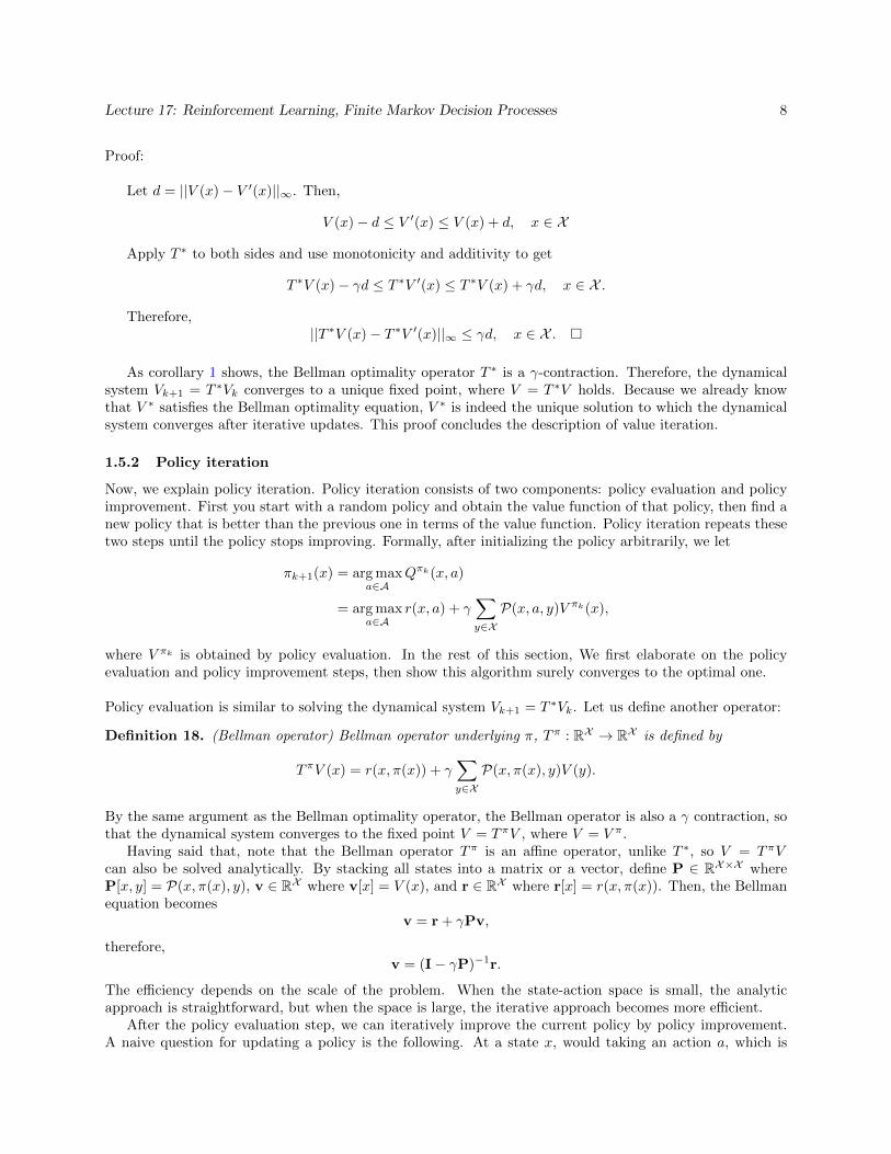
Proof:

Let d = ||V (x)− V ′(x)||∞. Then,

V (x)− d ≤ V ′(x) ≤ V (x) + d, x ∈ X

Apply T ∗ to both sides and use monotonicity and additivity to get

T ∗V (x)− γd ≤ T ∗V ′(x) ≤ T ∗V (x) + γd, x ∈ X .

Therefore,||T ∗V (x)− T ∗V ′(x)||∞ ≤ γd, x ∈ X . �

As corollary 1 shows, the Bellman optimality operator T ∗ is a γ-contraction. Therefore, the dynamicalsystem Vk+1 = T ∗Vk converges to a unique fixed point, where V = T ∗V holds. Because we already knowthat V ∗ satisfies the Bellman optimality equation, V ∗ is indeed the unique solution to which the dynamicalsystem converges after iterative updates. This proof concludes the description of value iteration.

1.5.2 Policy iteration

Now, we explain policy iteration. Policy iteration consists of two components: policy evaluation and policyimprovement. First you start with a random policy and obtain the value function of that policy, then find anew policy that is better than the previous one in terms of the value function. Policy iteration repeats thesetwo steps until the policy stops improving. Formally, after initializing the policy arbitrarily, we let

πk+1(x) = arg maxa∈A

Qπk(x, a)

= arg maxa∈A

r(x, a) + γ∑y∈XP(x, a, y)V πk(x),

where V πk is obtained by policy evaluation. In the rest of this section, We first elaborate on the policyevaluation and policy improvement steps, then show this algorithm surely converges to the optimal one.

Policy evaluation is similar to solving the dynamical system Vk+1 = T ∗Vk. Let us define another operator:

Definition 18. (Bellman operator) Bellman operator underlying π, Tπ : RX → RX is defined by

TπV (x) = r(x, π(x)) + γ∑y∈XP(x, π(x), y)V (y).

By the same argument as the Bellman optimality operator, the Bellman operator is also a γ contraction, sothat the dynamical system converges to the fixed point V = TπV , where V = V π.

Having said that, note that the Bellman operator Tπ is an affine operator, unlike T ∗, so V = TπVcan also be solved analytically. By stacking all states into a matrix or a vector, define P ∈ RX×X whereP[x, y] = P(x, π(x), y), v ∈ RX where v[x] = V (x), and r ∈ RX where r[x] = r(x, π(x)). Then, the Bellmanequation becomes

v = r + γPv,

therefore,v = (I− γP)−1r.

The efficiency depends on the scale of the problem. When the state-action space is small, the analyticapproach is straightforward, but when the space is large, the iterative approach becomes more efficient.

After the policy evaluation step, we can iteratively improve the current policy by policy improvement.A naive question for updating a policy is the following. At a state x, would taking an action a, which is


different from the current policy π(x), increase the expected return? In other words, is Qπ(x, a) greaterthan V π(x)? If so, intuitively, it would be better to have a new policy π′ that selects a every time when x isencountered, i.e. π′(x) = a. This intuition is correct and can be proved as a special case of a general resultcalled the policy improvement theorem. See [5] for the proof.

Proposition 1. (Policy improvement) Let π and π′ be any pair of deterministic policies such that,

Qπ(x, π′(x)) ≥ V π(x), ∀x.

Then the policy π′ must be as good as, or better than, π. That is, it must obtain greater or equal expectedreturn from all states x ∈ X :

V π′(x) ≥ V π(x).

This result can be applied to updates in all states and all possible actions. We can consider selecting ateach state the action that appears the best according to Qπ(x, a), i.e. following the new greedy policyπ′(x) = arg maxaQ

π(x, a). According to the proposition 1, the greedy policy is no worse than the originalpolicy.

Once a policy, π, has been improved using V π to yield a better policy, π′, we can then compute V π′

and improve the policy again to yield an even better π′′. We can thus obtain a sequence of monotonicallyimproving policies by repetition of policy evaluation and policy improvement. Because a finite MDP has onlya finite number of policies, this process must converge to an optimal policy in a finite number of iterations.

1.5.3 Value iteration vs. policy iteration

Finally, we present the pseudo code for value iteration and policy iteration and a brief analysis.

Algorithm 1 Value iteration

Require: P is the state transition probability kernel, r is the immediate reward function1. Initialize array V arbitrarily2. Update values for each state until convergencewhile ∆ > ε do

∆← 0for each x ∈ X do

U(x)← V (x)V (x)← maxa∈A

{r(x, a) + γ

∑y∈X P(x, a, y)U(y)

}∆← max(∆, |U(x)− V (x)|)

end forend while3. Output a deterministic policy, π, such that

π(x) = arg maxa∈A

{r(x, a) + γ


}

Value iteration is obtained by applying the Bellman optimality operator to the value function in aniterative manner (algorithm 1, step 2), and it eventually converges to the optimal value. We can get theoptimal policy out of it as the one that is greedy with respect to the optimal value function for every state(algorithm 1, step 3).


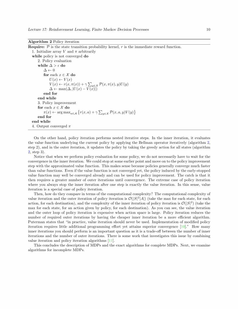
Algorithm 2 Policy iteration

Require: P is the state transition probability kernel, r is the immediate reward function.1. Initialize array V and π arbitrarilywhile policy is not converged do

2. Policy evaluationwhile ∆ > ε do

∆← 0for each x ∈ X do

U(x)← V (x)V (x)← r(x, π(x)) + γ

∑y∈X P(x, π(x), y)U(y)

∆← max(∆, |U(x)− V (x)|)end for

end while3. Policy improvementfor each x ∈ X do

π(x)← arg maxa∈A{r(x, a) + γ

∑y∈X P(x, a, y)V (y)

}end for

end while4. Output converged π

On the other hand, policy iteration performs nested iterative steps. In the inner iteration, it evaluatesthe value function underlying the current policy by applying the Bellman operator iteratively (algorithm 2,step 2), and in the outer iteration, it updates the policy by taking the greedy action for all states (algorithm2, step 3).

Notice that when we perform policy evaluation for some policy, we do not necessarily have to wait for theconvergence in the inner iteration. We could stop at some earlier point and move on to the policy improvementstep with the approximated value function. This makes sense because policies generally converge much fasterthan value functions. Even if the value function is not converged yet, the policy induced by the early-stoppedvalue function may well be converged already and can be used for policy improvement. The catch is that itthen requires a greater number of outer iterations until convergence. The extreme case of policy iterationwhere you always stop the inner iteration after one step is exactly the value iteration. In this sense, valueiteration is a special case of policy iteration.

Then, how do they compare in terms of the computational complexity? The computational complexity ofvalue iteration and the outer iteration of policy iteration is O(|S|2|A|) (take the max for each state, for eachaction, for each destination), and the complexity of the inner iteration of policy iteration is O(|S|2) (take themax for each state, for an action given by policy, for each destination). As you can see, the value iterationand the outer loop of policy iteration is expensive when action space is large. Policy iteration reduces thenumber of required outer iterations by having the cheaper inner iteration be a more efficient algorithm.Puterman states that “in practice, value iteration should never be used. Implementation of modified policyiteration requires little additional programming effort yet attains superior convergence [10].” How manyinner iterations you should perform is an important question as it is a trade-off between the number of inneriterations and the number of outer iterations. There is some work that investigates this issue by combiningvalue iteration and policy iteration algorithms [11].

This concludes the description of MDPs and the exact algorithms for complete MDPs. Next, we examinealgorithms for incomplete MDPs.


2 Reinforcement learning

2.1 Predicting value functions

In reinforcement learning, if a perfect model is not thrown, meaning, an MDP is not be completely specified,then we need to apply some estimation methods to predict the model before policy iteration. In this section,we consider the problem of estimating the value function underlying an MRP (see definition 7). An MRParises when you fix a policy π for your MDP.

Value prediction problems arise in a number of ways: Estimating the probability of some future event,the expected time until some event occurs, or the (action-)value function underlying some policy in an MDPare all value prediction problems. Specific applications include estimating the failure probability of a largepower grid [12] or estimating taxi-out times of flights at busy airports [13].

The value of a state is defined as the expectation of the random return when the process is startedfrom the given state. The so-called Monte-Carlo method computes an average over multiple independentrealizations started from each state to estimate this value for each state. However, this method can sufferfrom high variance of the returns, which means the quality of estimates could be poor. Also, when interactingwith a system in a closed-loop fashion (i.e., when estimation happens while interacting with the system), itmight be impossible to reset the state of the system to some particular state. In this case, the Monte-Carlotechnique cannot be applied without introducing some additional bias. Temporal difference (TD) learningis a method that can be used to address these issues.

2.1.1 TD in finite state spaces

The unique feature of TD learning is that it uses bootstrapping: predictions are used as targets duringthe course of learning. In this section, we first introduce the most basic TD(0) algorithm and explainhow bootstrapping works (see Algorithm 3). Next, we compare TD learning to Monte-Carlo methods (seeAlgorithm 4). Finally, we present the TD(λ) algorithm that unifies the two approaches (see Algorithm 5),where λ is a hyperparameter of the algorithms.

Here we consider only the case of finite MRPs, when computing the value-estimates of all the states iscomputationally intractable. This is known as the tabular case in the reinforcement learning literature. Wewill discuss the infinite case in section 2.1.2.

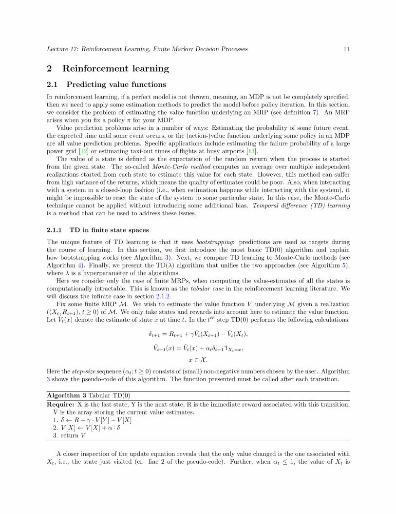
Fix some finite MRP M. We wish to estimate the value function V underlying M given a realization((Xt, Rt+1), t ≥ 0) ofM. We only take states and rewards into account here to estimate the value function.Let Vt(x) denote the estimate of state x at time t. In the tth step TD(0) performs the following calculations:

δt+1 = Rt+1 + γVt(Xt+1)− Vt(Xt),

Vt+1(x) = Vt(x) + αtδt+11Xt=x,

x ∈ X .

Here the step-size sequence (αt; t ≥ 0) consists of (small) non-negative numbers chosen by the user. Algorithm3 shows the pseudo-code of this algorithm. The function presented must be called after each transition.

Algorithm 3 Tabular TD(0)

Require: X is the last state, Y is the next state, R is the immediate reward associated with this transition,V is the array storing the current value estimates.1. δ ← R+ γ · V [Y ]− V [X]2. V [X]← V [X] + α · δ3. return V

A closer inspection of the update equation reveals that the only value changed is the one associated withXt, i.e., the state just visited (cf. line 2 of the pseudo-code). Further, when αt ≤ 1, the value of Xt is


moved towards the target Rt+1 + γVt(Xt+1). Since the target depends on the estimated value function, thealgorithm uses bootstrapping. The term temporal difference in the name of the algorithm comes from thatδt+1 is defined as the difference between values of states corresponding to successive time steps.

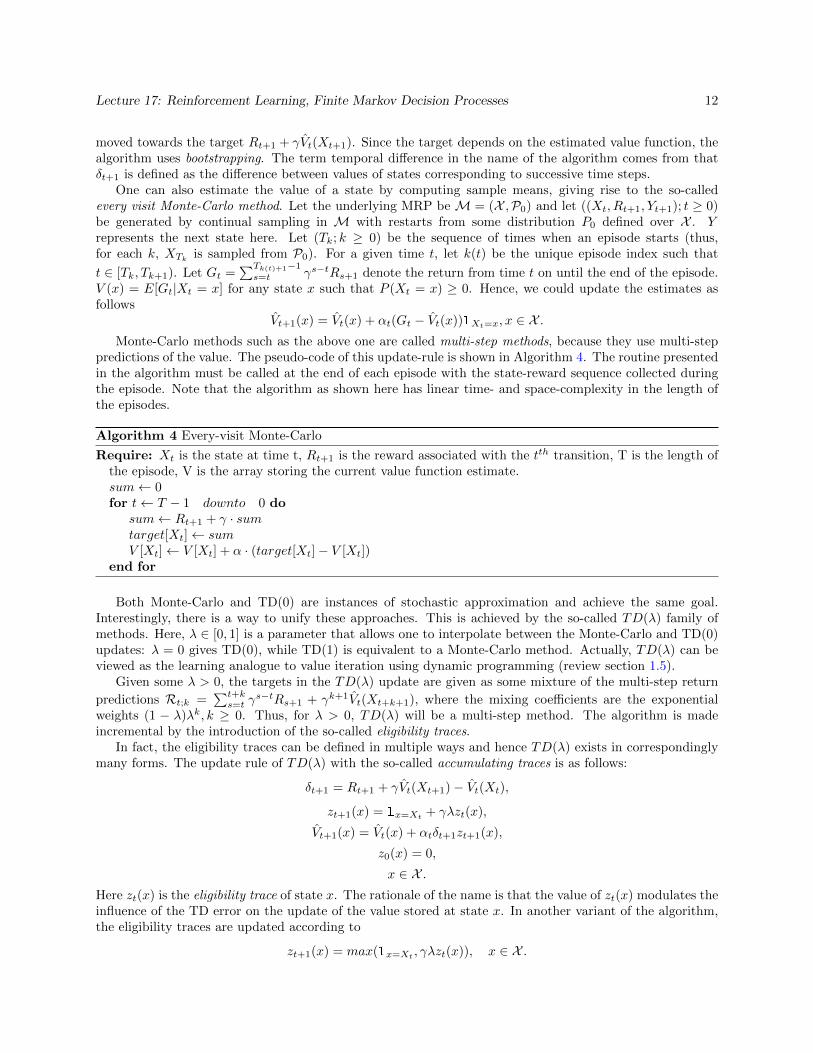
One can also estimate the value of a state by computing sample means, giving rise to the so-calledevery visit Monte-Carlo method. Let the underlying MRP be M = (X ,P0) and let ((Xt, Rt+1, Yt+1); t ≥ 0)be generated by continual sampling in M with restarts from some distribution P0 defined over X . Yrepresents the next state here. Let (Tk; k ≥ 0) be the sequence of times when an episode starts (thus,for each k, XTk is sampled from P0). For a given time t, let k(t) be the unique episode index such that

t ∈ [Tk, Tk+1). Let Gt =∑Tk(t)+1−1s=t γs−tRs+1 denote the return from time t on until the end of the episode.

V (x) = E[Gt|Xt = x] for any state x such that P (Xt = x) ≥ 0. Hence, we could update the estimates asfollows

Vt+1(x) = Vt(x) + αt(Gt − Vt(x))1Xt=x, x ∈ X .Monte-Carlo methods such as the above one are called multi-step methods, because they use multi-step

predictions of the value. The pseudo-code of this update-rule is shown in Algorithm 4. The routine presentedin the algorithm must be called at the end of each episode with the state-reward sequence collected duringthe episode. Note that the algorithm as shown here has linear time- and space-complexity in the length ofthe episodes.

Algorithm 4 Every-visit Monte-Carlo

Require: Xt is the state at time t, Rt+1 is the reward associated with the tth transition, T is the length ofthe episode, V is the array storing the current value function estimate.sum← 0for t← T − 1 downto 0 do

sum← Rt+1 + γ · sumtarget[Xt]← sumV [Xt]← V [Xt] + α · (target[Xt]− V [Xt])

end for

Both Monte-Carlo and TD(0) are instances of stochastic approximation and achieve the same goal.Interestingly, there is a way to unify these approaches. This is achieved by the so-called TD(λ) family ofmethods. Here, λ ∈ [0, 1] is a parameter that allows one to interpolate between the Monte-Carlo and TD(0)updates: λ = 0 gives TD(0), while TD(1) is equivalent to a Monte-Carlo method. Actually, TD(λ) can beviewed as the learning analogue to value iteration using dynamic programming (review section 1.5).

Given some λ > 0, the targets in the TD(λ) update are given as some mixture of the multi-step return

predictions Rt;k =∑t+ks=t γ

s−tRs+1 + γk+1Vt(Xt+k+1), where the mixing coefficients are the exponentialweights (1 − λ)λk, k ≥ 0. Thus, for λ > 0, TD(λ) will be a multi-step method. The algorithm is madeincremental by the introduction of the so-called eligibility traces.

In fact, the eligibility traces can be defined in multiple ways and hence TD(λ) exists in correspondinglymany forms. The update rule of TD(λ) with the so-called accumulating traces is as follows:

δt+1 = Rt+1 + γVt(Xt+1)− Vt(Xt),

zt+1(x) = 1x=Xt + γλzt(x),

Vt+1(x) = Vt(x) + αtδt+1zt+1(x),

z0(x) = 0,

x ∈ X .Here zt(x) is the eligibility trace of state x. The rationale of the name is that the value of zt(x) modulates theinfluence of the TD error on the update of the value stored at state x. In another variant of the algorithm,the eligibility traces are updated according to

zt+1(x) = max(1x=Xt , γλzt(x)), x ∈ X .


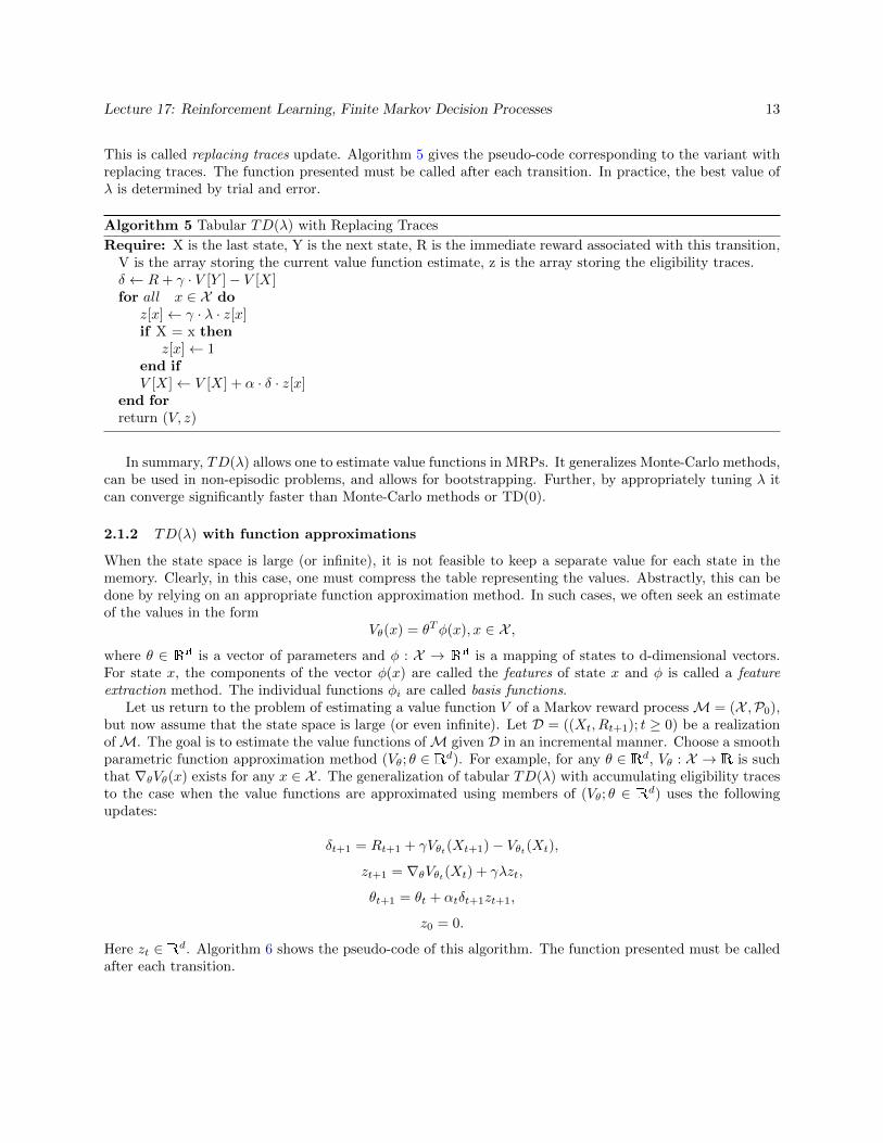
This is called replacing traces update. Algorithm 5 gives the pseudo-code corresponding to the variant withreplacing traces. The function presented must be called after each transition. In practice, the best value ofλ is determined by trial and error.

Algorithm 5 Tabular TD(λ) with Replacing Traces

Require: X is the last state, Y is the next state, R is the immediate reward associated with this transition,V is the array storing the current value function estimate, z is the array storing the eligibility traces.δ ← R+ γ · V [Y ]− V [X]for all x ∈ X do

z[x]← γ · λ · z[x]if X = x then

z[x]← 1end ifV [X]← V [X] + α · δ · z[x]

end forreturn (V, z)

In summary, TD(λ) allows one to estimate value functions in MRPs. It generalizes Monte-Carlo methods,can be used in non-episodic problems, and allows for bootstrapping. Further, by appropriately tuning λ itcan converge significantly faster than Monte-Carlo methods or TD(0).

2.1.2 TD(λ) with function approximations

When the state space is large (or infinite), it is not feasible to keep a separate value for each state in thememory. Clearly, in this case, one must compress the table representing the values. Abstractly, this can bedone by relying on an appropriate function approximation method. In such cases, we often seek an estimateof the values in the form

Vθ(x) = θTφ(x), x ∈ X ,

where θ ∈ Rd is a vector of parameters and φ : X → Rd is a mapping of states to d-dimensional vectors.

For state x, the components of the vector φ(x) are called the features of state x and φ is called a featureextraction method. The individual functions φi are called basis functions.

Let us return to the problem of estimating a value function V of a Markov reward processM = (X ,P0),but now assume that the state space is large (or even infinite). Let D = ((Xt, Rt+1); t ≥ 0) be a realizationofM. The goal is to estimate the value functions ofM given D in an incremental manner. Choose a smoothparametric function approximation method (Vθ; θ ∈ Rd). For example, for any θ ∈ Rd, Vθ : X → R is suchthat ∇θVθ(x) exists for any x ∈ X . The generalization of tabular TD(λ) with accumulating eligibility tracesto the case when the value functions are approximated using members of (Vθ; θ ∈ Rd) uses the followingupdates:

δt+1 = Rt+1 + γVθt(Xt+1)− Vθt(Xt),

zt+1 = ∇θVθt(Xt) + γλzt,

θt+1 = θt + αtδt+1zt+1,

z0 = 0.

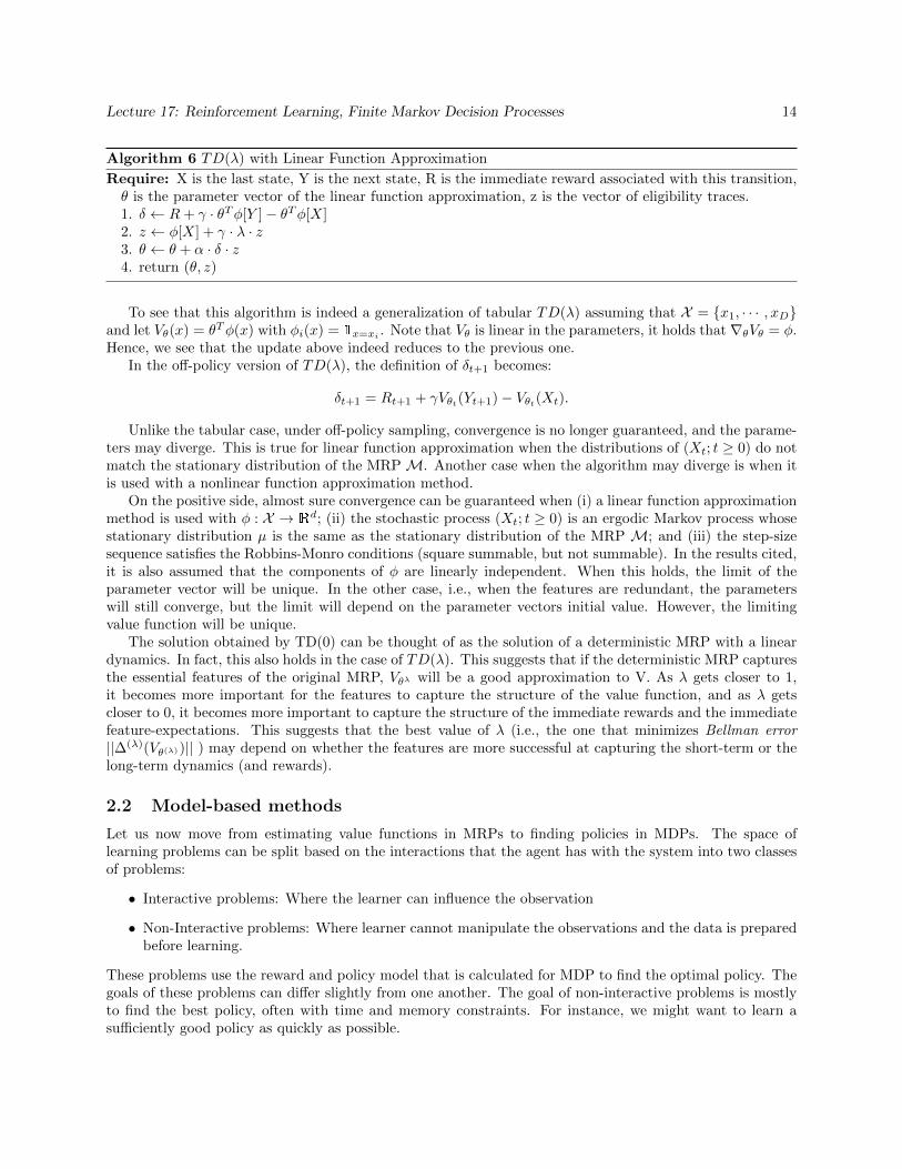
Here zt ∈ Rd. Algorithm 6 shows the pseudo-code of this algorithm. The function presented must be calledafter each transition.


Algorithm 6 TD(λ) with Linear Function Approximation

Require: X is the last state, Y is the next state, R is the immediate reward associated with this transition,θ is the parameter vector of the linear function approximation, z is the vector of eligibility traces.1. δ ← R+ γ · θTφ[Y ]− θTφ[X]2. z ← φ[X] + γ · λ · z3. θ ← θ + α · δ · z4. return (θ, z)

To see that this algorithm is indeed a generalization of tabular TD(λ) assuming that X = {x1, · · · , xD}and let Vθ(x) = θTφ(x) with φi(x) = 1x=xi . Note that Vθ is linear in the parameters, it holds that ∇θVθ = φ.Hence, we see that the update above indeed reduces to the previous one.

In the off-policy version of TD(λ), the definition of δt+1 becomes:

δt+1 = Rt+1 + γVθt(Yt+1)− Vθt(Xt).

Unlike the tabular case, under off-policy sampling, convergence is no longer guaranteed, and the parame-ters may diverge. This is true for linear function approximation when the distributions of (Xt; t ≥ 0) do notmatch the stationary distribution of the MRPM. Another case when the algorithm may diverge is when itis used with a nonlinear function approximation method.

On the positive side, almost sure convergence can be guaranteed when (i) a linear function approximationmethod is used with φ : X → R

d; (ii) the stochastic process (Xt; t ≥ 0) is an ergodic Markov process whosestationary distribution µ is the same as the stationary distribution of the MRP M; and (iii) the step-sizesequence satisfies the Robbins-Monro conditions (square summable, but not summable). In the results cited,it is also assumed that the components of φ are linearly independent. When this holds, the limit of theparameter vector will be unique. In the other case, i.e., when the features are redundant, the parameterswill still converge, but the limit will depend on the parameter vectors initial value. However, the limitingvalue function will be unique.

The solution obtained by TD(0) can be thought of as the solution of a deterministic MRP with a lineardynamics. In fact, this also holds in the case of TD(λ). This suggests that if the deterministic MRP capturesthe essential features of the original MRP, Vθλ will be a good approximation to V. As λ gets closer to 1,it becomes more important for the features to capture the structure of the value function, and as λ getscloser to 0, it becomes more important to capture the structure of the immediate rewards and the immediatefeature-expectations. This suggests that the best value of λ (i.e., the one that minimizes Bellman error||∆(λ)(Vθ(λ))|| ) may depend on whether the features are more successful at capturing the short-term or thelong-term dynamics (and rewards).

2.2 Model-based methods

Let us now move from estimating value functions in MRPs to finding policies in MDPs. The space oflearning problems can be split based on the interactions that the agent has with the system into two classesof problems:

• Interactive problems: Where the learner can influence the observation

• Non-Interactive problems: Where learner cannot manipulate the observations and the data is preparedbefore learning.

These problems use the reward and policy model that is calculated for MDP to find the optimal policy. Thegoals of these problems can differ slightly from one another. The goal of non-interactive problems is mostlyto find the best policy, often with time and memory constraints. For instance, we might want to learn asufficiently good policy as quickly as possible.


Interactive learning problems can be further split up based on their goals. The first class of problems areonline learning problems, whose goal is to increase online performance, such as number of optimal solutionsor reward gain.

Another category of interactive problems is active learning. Its goal is to find the best policy for theproblem, similar to the non-interactive problems. The main difference between the two category is that inactive learning problems, the agent can influence the input in favor of finding a better policy. Specifically,based on what examples have been seen so far, the agent can adjust its sampling strategy more towardseither exploration exploitation.

In the following section we will consider problems of online learning and active learning, for the bothscenario of having a bandit(i.e. an MDP with single state) and normal MDPs.

2.2.1 Online learning in Bandits

In this section we first look closely at the problem of online learning in bandits. Bandits are MDPs with onlyone state and multiple actions. Once we have learned an optimal value function, we want to follow a greedyapproach to guarantee the best results. However, during training, before the value function has converged,taking a greedy approach can cause the learner to get stuck in a local optimum. Thus each learner shouldbe able to explore by trying sub-optimal actions. However, we also don’t want the learner to spend all itstime taking sub-optimal actions, so we want to limit how many explore actions the learner takes. There area variety of methods for choosing how to balance exploration and exploitation.

ε-Greedy Method In this method we choose to explore with probability of some ε ∈ [0, 1]. Specifically,with probability ε take a random action, and with probability 1 − ε take the optimal action. Typically, εdecays over time, allowing the learner to eventually hone in on the optimal policy.

Boltzmann exploration The main difference between this strategy and the ε-Greedy one is that in thismethod we can take the values of each action into account. With this strategy the action at each stage ischosen according to the following distribution:

π(a) =exp(βQt(a))∑

a′∈A exp(βQt(a′))

In the equation above, Qt(a) is the sample mean of action a up to time t, and β is a parameter thatdetermines the exploration-exploitation trade-off. The intuition behind this formula is to weight actionsaccording to their relative values. Higher values of β result in a greedier policy, with β →∞ resulting in thegreedy policy of always selecting the optimal action.

Optimism in the face of uncertainty While the previous two approaches can be competitive withmore complicated methods, there is no known automated way of properly adjusting the parameters ε or βto achieve optimal performance. This approach is potentially a better implementation of the exploration-exploitation strategy. According to this strategy the learner should choose an action that has the highestvalue for the upper confidence bound. The main intuition is to check the history of each action and choosethem based on how well they get rewarded over a period of time with consideration of the current reward.There are different method for calculating the upper bound but the best one is UCB1. According to thatthe upper bound can be computed as below.

Ut(a) = rt(a) +R

√2 log t

nt(a)

In the equation above nt(a) is the number of times that action a is chosen until time t, rt(a) shows theaverage reward of taking action a until time t, and R is an upper bound for the observed rewards. If weknow that the variance of reward values are not high we can replace R with estimates of the variance as


it will be a better upper bound. Using this UCB as a sampling strategy is done in two stages: select andupdate. In the select phase, we choose the action that has the highest upper bound. During the update stagewe update the count and average reward based on the selected action.

2.2.2 Online learning in MDPs

Now lets consider the problem of online learning for MDPs. The goal that we are pursuing here is to minimizethe regret. Regret is the difference between the total reward that our learner receives and the optimal rewardthat the learner could have received. Let’s consider the MDP that has all the states connected (unichain)and the immediate rewards are all in the interval of [0,1]. For a fixed policy, π on this MDP, we can definea stationary distribution over the states which we will call µπ(x). Therefore the average reward for policy πwould be:

ρπ =∑x∈X

(µπ(x))(r(x, π(x)))

Here r is the reward function for taking action π(x) at state x. If we call the optimal long-time rewardρ∗ = arg max

πρπ then we can define the regret to be:

RAT = Tρ∗ −RAT

In equation above RAT is regret and RAT is the reward of using some learning algorithm A until time T .

As can be seen above, minimizing the regret is exactly maximizing the total reward obtained over time.

UCRL2 There exists an algorithm called UCRL2 [14] that achieves logarithmic regret with respect totime. In order to describe this algorithm in detail we have to go over some definitions:

Definition 19. (Diameter) The diameter is the largest number of steps, in expectation under a policyminimizes the number of steps, that is needed to get to some state starting from some other state. In otherwords this is a longest path in the markov chain. Note that if an MDP has any states that are not reachablefrom some other state, the diameter is infinite.

Definition 20. (Gap) The gap is the difference between the optimal policy and the second optimal perfor-mance.

By setting the confidence parameter to λ = 1/(3T ), the expected regret of the UCLR2 algorithm is:

E[RUCRL2(λ)T ] = O(

D2|X|2|A| log(T )

g)

Where D is the diameter of the MDP, and g is the gap. This expected regret can be used in the situationswhere we have a high value for g. For small g since the value of the expected regret gets large there wouldbe no point for using the bound with small T . In those cases there is an alternative expected regret definedas:

E[RUCRL2(λ)T ] = O(D|X|

√|A|T log(T ))

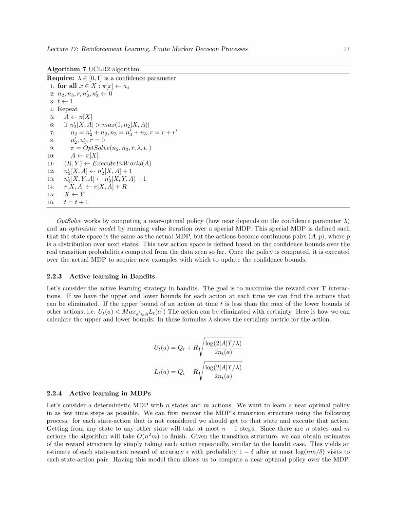
UCRL2 algorithm has two steps. In the first step each action is executed and the next state and reward arecalculated. This algorithm constructs confidence intervals around the estimates of the transition probabilitiesand immediate reward function. These define a set of plausible MDPs. One upside of this algorithm is thatit waits to update the policy until sufficient information has been obtained, as can be seen in line 6 of thepseudo-code below. Here, n2 is a counter for (state, action) pairs, n3 is a counter for (state, action, nextstate) triples. n′2 and n′3 count the number of times each pair/triple has been seen since the last update. rkeeps track of the rewards obtained for starting with each (state, action) pair.


Algorithm 7 UCLR2 algorithm.

Require: λ ∈ [0, 1] is a confidence parameter1: for all x ∈ X : π[x]← a12: n2, n3, r, n

′2, n′3 ← 0

3: t← 14: Repeat5: A← π[X]6: if n′2[X,A] > max(1, n2[X,A])7: n2 = n′2 + n2, n3 = n′3 + n3, r = r + r′

8: n′2, n′3, r = 0

9: π = OptSolve(n2, n3, r, λ, t, )10: A← π[X]11: (R, Y )← ExecuteInWorld(A)12: n′2[X,A]← n′2[X,A] + 113: n′3[X,Y,A]← n′3[X,Y,A] + 114: r[X,A]← r[X,A] +R15: X ← Y16: t = t+ 1

OptSolve works by computing a near-optimal policy (how near depends on the confidence parameter λ)and an optimistic model by running value iteration over a special MDP. This special MDP is defined suchthat the state space is the same as the actual MDP, but the actions become continuous pairs (A, p), where pis a distribution over next states. This new action space is defined based on the confidence bounds over thereal transition probabilities computed from the data seen so far. Once the policy is computed, it is executedover the actual MDP to acquire new examples with which to update the confidence bounds.

2.2.3 Active learning in Bandits

Let’s consider the active learning strategy in bandits. The goal is to maximize the reward over T interac-tions. If we have the upper and lower bounds for each action at each time we can find the actions thatcan be eliminated. If the upper bound of an action at time t is less than the max of the lower bounds ofother actions, i.e. Ut(a) < Maxa′∈ALt(a

′) The action can be eliminated with certainty. Here is how we can

calculate the upper and lower bounds: In these formulas λ shows the certainty metric for the action.

Ut(a) = Qt +R

√log(2|A|T/λ)

2nt(a)

Lt(a) = Qt −R

√log(2|A|T/λ)

2nt(a)

2.2.4 Active learning in MDPs

Let’s consider a deterministic MDP with n states and m actions. We want to learn a near optimal policyin as few time steps as possible. We can first recover the MDP’s transition structure using the followingprocess: for each state-action that is not considered we should get to that state and execute that action.Getting from any state to any other state will take at most n − 1 steps. Since there are n states and mactions the algorithm will take O(n2m) to finish. Given the transition structure, we can obtain estimatesof the reward structure by simply taking each action repeatedly, similar to the bandit case. This yields anestimate of each state-action reward of accuracy ε with probability 1 − δ after at most log(nm/δ) visits toeach state-action pair. Having this model then allows us to compute a near optimal policy over the MDP.


Specifically, we can compute an ε-optimal policy in at most n2m + 4e log(nm/δ)/((1 − γ)2ε)2 steps, wheree ≤ n2m is the number of time steps to visit all state-action pairs.

There is currently no similar result for active learning in stochastic MDPs.

2.3 Model-free methods

Let us now discuss a set of methods that approximate the action-value function, Q(x, a), directly, rather thanestimating the state-value function, V (x). Because these methods directly learn the action-value functionwithout estimating a model of the MDP’s transition or reward structures, they are known as “Model-free”approaches.

Assuming we are able to learn a near-optimal Q function, we can give a lower bound on value of a policy,π that is greedy w.r.t. Q. As shown in [15], the value of policy π can be bounded as follows:

V π(x) ≥ V ∗(x)− 2

1− γ||Q−Q∗||∞ , x ∈ X

Which shows that as the learned Q function approaches Q∗, the value, V π of following a greedy policy withrespect to the laerned Q function approaches V ∗.

2.3.1 Q-learning

The first model-free approach for learning policies is Q-learning. Similar to the methods described above,Q-learning can be applied in both finite and infinite MDPs. We first look at the finite setting, and thengeneralize that with various function approximations to apply the approach to the infinite setting.

Finite MDPs Q-learning was first introduced in [16], and uses the TD approach to estimate the Qfunction. Upon observing a transition (Xt, At, Rt+1, Yt+1), the estimates are updated as follows:

δt+1(Q) = Rt+1 + γ maxa′∈A

Q(Yt+1, a′)−Q(Xt, At),

Qt+1(x, a) = Qt(x, a) + αtδt+1(Qt)1{x=Xt,a=At}

It is proven in [?] that the above updates will converge if appropriate learning rates, αt are used. It issimple to see that when it converges, it converges to the optimal Q∗. At convergence, it is necessary thatE[δt+1(Q)|Xt, At] = 0. Using the fact that (Yt+1, Rt+1) ∼ P0(·|Xt, At), we can break this expectation downas follows

E[δt+1(Q)|Xt, At] = E[Rt+1 + γ maxa′∈A

Qt(Yt+1, a′)−Qt(Xt, At)]

= r(Xt, At) + γ∑y∈XP(Xt, At, y) sup

a′∈AQt(y, a

′)−Qt(Xt, At)

= T ∗Qt(Xt, At)−Qt(Xt, At)

Thus, when these updates converge, we get that T ∗Qt(x, a) = Qt(x, a), which is satisfied by Qt = Q∗.Additionally, using the above equation, we can see that

E[Qt+1(Xt, At)|Xt, At] = (1− αt)Qt(Xt, At) + αtT∗Qt(Xt, At)

which shows that the expected update at each timestep is simply taking steps according to the Bellmanoptimality operator given the observed state-action pair.

Some of the benefits of Q-learning include its simplicity, as well as the fact that it is able to make use ofarbitrary training data, as long as in the limit all state-action pairs are updated infinitely often. Similar tothe exploration-exploitation trade-off seen in section 2.2.1, ε-greedy or Boltzmann approaches are often usedto sample actions in the closed-loop setting.


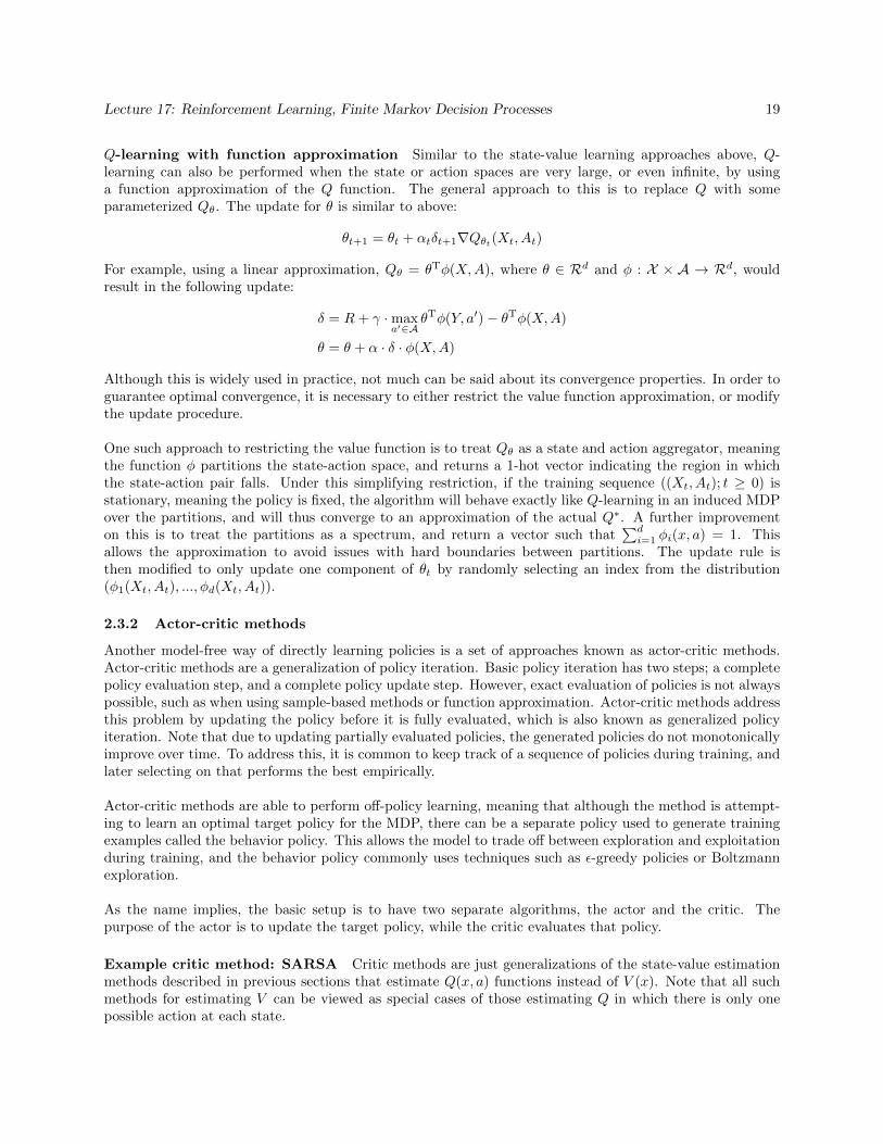
Q-learning with function approximation Similar to the state-value learning approaches above, Q-learning can also be performed when the state or action spaces are very large, or even infinite, by usinga function approximation of the Q function. The general approach to this is to replace Q with someparameterized Qθ. The update for θ is similar to above:

θt+1 = θt + αtδt+1∇Qθt(Xt, At)

For example, using a linear approximation, Qθ = θTφ(X,A), where θ ∈ Rd and φ : X × A → Rd, wouldresult in the following update:

δ = R+ γ ·maxa′∈A

θTφ(Y, a′)− θTφ(X,A)

θ = θ + α · δ · φ(X,A)

Although this is widely used in practice, not much can be said about its convergence properties. In order toguarantee optimal convergence, it is necessary to either restrict the value function approximation, or modifythe update procedure.

One such approach to restricting the value function is to treat Qθ as a state and action aggregator, meaningthe function φ partitions the state-action space, and returns a 1-hot vector indicating the region in whichthe state-action pair falls. Under this simplifying restriction, if the training sequence ((Xt, At); t ≥ 0) isstationary, meaning the policy is fixed, the algorithm will behave exactly like Q-learning in an induced MDPover the partitions, and will thus converge to an approximation of the actual Q∗. A further improvementon this is to treat the partitions as a spectrum, and return a vector such that

∑di=1 φi(x, a) = 1. This

allows the approximation to avoid issues with hard boundaries between partitions. The update rule isthen modified to only update one component of θt by randomly selecting an index from the distribution(φ1(Xt, At), ..., φd(Xt, At)).

2.3.2 Actor-critic methods

Another model-free way of directly learning policies is a set of approaches known as actor-critic methods.Actor-critic methods are a generalization of policy iteration. Basic policy iteration has two steps; a completepolicy evaluation step, and a complete policy update step. However, exact evaluation of policies is not alwayspossible, such as when using sample-based methods or function approximation. Actor-critic methods addressthis problem by updating the policy before it is fully evaluated, which is also known as generalized policyiteration. Note that due to updating partially evaluated policies, the generated policies do not monotonicallyimprove over time. To address this, it is common to keep track of a sequence of policies during training, andlater selecting on that performs the best empirically.

Actor-critic methods are able to perform off-policy learning, meaning that although the method is attempt-ing to learn an optimal target policy for the MDP, there can be a separate policy used to generate trainingexamples called the behavior policy. This allows the model to trade off between exploration and exploitationduring training, and the behavior policy commonly uses techniques such as ε-greedy policies or Boltzmannexploration.

As the name implies, the basic setup is to have two separate algorithms, the actor and the critic. Thepurpose of the actor is to update the target policy, while the critic evaluates that policy.

Example critic method: SARSA Critic methods are just generalizations of the state-value estimationmethods described in previous sections that estimate Q(x, a) functions instead of V (x). Note that all suchmethods for estimating V can be viewed as special cases of those estimating Q in which there is only onepossible action at each state.


One such method is SARSA, named such due to making use of the current State, current Action, nextReward, next State, and next Action. Basic SARSA is just TD(0) applied to state-action pairs, and can beused to evaluate a specific policy. It follows the update below.

δt+1(Q) = Rt+1 +Q(Yt+1, At+1)−Q(Xt, At)

Qt+1(x, a) = Qt(x, a) + αtδt+1(Qt)1{x=Xt,a=At}

This is very similar to Q-learning. The primary difference is that SARSA updates the Q function basedon the next action taken according to the behavior policy, while Q-learning uses the greedy action. Thispotentially results in slightly different convergence values. For example, using an ε-greedy behavior policywith fixed ε, the expected value under Q-learning will be the optimal action value, Q(st, at) = max

aQ(st, a),

while the expected value under SARSA is the weighted sum of the average action value and the optimalaction value, Q(st, at) = ε

∑aQ(st, a) + (1− ε) max

aQ(st, a).

Additionally, as SARSA is just TD(0) for state-action pairs, it can be also be extended to SARSA(λ), anduse function approximation. These extensions are subject to the same limitations as in the TD(λ) case.

Example actor method: Greedy policy improvement The actor portion of actor-critic methods isresponsible for improving a policy given the results of the critic’s evaluation. The simplest such method is tosimply take a greedy approach w.r.t. the action-value function returned by the critic. Note that with finiteaction space, this policy can be computed as needed, allowing it to run in very large state spaces.

References

[1] Richard Bellman. A markovian decision process. Journal of Mathematics and Mechanics, pages 679–684,1957.

[2] Ronald A Howard. Dynamic programming and Markov processes. Wiley for The Massachusetts Instituteof Technology, 1964.

[3] Peter Auer, Nicolo Cesa-Bianchi, and Paul Fischer. Finite-time analysis of the multiarmed banditproblem. Machine learning, 47(2-3):235–256, 2002.

[4] William R Thompson. On the likelihood that one unknown probability exceeds another in view of theevidence of two samples. Biometrika, 25(3/4):285–294, 1933.

[5] Csaba Szepesvari. Algorithms for reinforcement learning. Synthesis lectures on artificial intelligenceand machine learning, 4(1):1–103, 2010.

[6] Eugene A Feinberg. Total expected discounted reward mdps: existence of optimal policies. WileyEncyclopedia of Operations Research and Management Science, 2011.

[7] Richard Bellman. Dynamic programming. Courier Corporation, 2013.

[8] Stuart Dreyfus. Richard bellman on the birth of dynamic programming. Operations Research, 50(1):48–51, 2002.

[9] Emo Todorov. Markov decision processes and bellman equations. 2014.

[10] Martin L Puterman. Markov decision processes: discrete stochastic dynamic programming. John Wiley& Sons, 2014.

[11] Elena Pashenkova, Irina Rish, and Rina Dechter. Value iteration and policy iteration algorithms formarkov decision problem. In AAAI96: Workshop on Structural Issues in Planning and Temporal Rea-soning. Citeseer, 1996.


[12] Mannor S. Frank, J. and D. Precup. Reinforcement learning in the presence of rare events. Proceedingsof the 25th In- ternational Conference Machine Learning (ICML 2008), 307.

[13] Ganesan R. Sherry L. Balakrishna, P. and B. Levy. Estimating taxi-out times with a reinforcementlearning algorithm. 27th IEEE/AIAA Digital Avionics Systems Conference, pages 3.D.3–1–3.D.3–12,2008.

[14] Peter Auer, Thomas Jaksch, and Ronald Ortner. Near-optimal regret bounds for reinforcement learning.Journal of Machine Learning Research, 11:1563–1600, 2010.

[15] Satinder P Singh and Richard C Yee. An upper bound on the loss from approximate optimal-valuefunctions. Machine Learning, 16(3):227–233, 1994.

[16] C. J. C. H. Watkins. Learning from Delayed Rewards. PhD thesis, King’s College, Cambridge, UK,1989.

Documents

CSE599i: Online and Adaptive Machine Learning Winter 2018 ...Lecture 17: Reinforcement Learning, Finite Markov Decision Processes 2 De nition 1. (Finite Markov decision processes)