1

REINFORCEMENT-FREE DECKS USING A MODIFIED STRUT-AND-TIE MODEL 1

2

Han Ug Bae, Michael G. Oliva, Lawrence C. Bank 3

Department of Civil and Environmental Engineering, University of Wisconsin-Madison, 2205 4

Engineering Hall, 1415 Engineering Drive, Madison, WI 53706. 5

6

Biography: Han Ug Bae is a postdoctoral fellow in Civil and Environmental Engineering at 7

University of Wisconsin-Madison. He received his BS and MS from Yonsei University, Seoul, 8

Korea and PhD from University of Wisconsin-Madison. His research interests include strut-and-tie 9

models, development of highway bridge design methods and bridge construction. 10

Michael G. Oliva is a Professor in the Department of Civil and Environmental Engineering at 11

University of Wisconsin-Madison. He received his BS from University of Wisconsin-Madison; MS 12

and PhD from University of California, Berkeley. His research interests include highway bridges, 13

reinforced-precast-prestressed concrete design and earthquake resistance. 14

ACI member Lawrence C. Bank is a Professor in the Department of Civil and Environmental 15

Engineering at University of Wisconsin-Madison. He received his BS from Technion- Israel 16

Institute of Technology, Haifa, Israel; MS and PhD from Columbia University. He is a member of 17

ACI committee 440 (Fiber Reinforced Polymer Reinforcement). His research interests include FRP 18

composites in structural engineering, mechanics of composite materials and innovative bridge 19

construction. 20

21

ABSTRACT 22

This paper describes an application of a modified strut-and-tie model (STM) for determining the 23

strength of reinforcement-free bridge decks on concrete wide flange girders. The method could also 24

be applied to other short span restrained concrete slabs. The concept presented for the 25

reinforcement-free bridge deck includes a combination of removing steel reinforcement, utilizing 26

2

compressive membrane action in the deck by tying girders together, and introducing a 1

polypropylene fiber to control shrinkage cracks. An analysis method for these reinforcement-free 2

decks using a modified STM that considers geometrical nonlinearity is proposed. The model 3

provides a 2D axisymmetric representation of the behavior of the reinforcement-free deck and it is 4

capable of capturing punching and flexural failure. Comparisons to nonlinear FEM analysis results 5

were made to verify the proposed analysis method. A design load appropriate for reinforcement-free 6

bridge decks is proposed. 7

8

Keywords: strut-and-tie model; reinforcement-free deck; punching shear; precast prestressed 9

girder; bridge decks; compressive membrane action; deck analysis; and wide flange concrete girder. 10

11

INTRODUCTION 12

The strut-and-tie model (STM) developed by Schlaich et al.1 is considered to be a powerful new 13

model for design and analysis of disturbed or discontinuous regions (D-regions) where geometrical 14

or structural complexity exists in concrete members. The model is recognized in ACI 3182 and 15

numerous investigations and modifications of the method have been performed.3-6 16

The STM can be used for a restrained short span bridge deck on girders since the deck behaves like 17

a D-region. Concentrated forces develop where the girder supports the deck and at the center of the 18

span under a wheel load. Compressive membrane action (CMA) develops in the restrained deck and 19

changes the failure mode from a flexural failure to a punching shear failure, enhancing the capacity, 20

if sufficient lateral restraint is provided.7 Lateral restraint in the deck around the loaded region 21

inhibits rotation, which is accompanied by translation in the plane of the deck, and leads to an 22

enhancement of the flexural capacity of the deck. Analysis methods to predict the enhanced 23

capacity of the restrained deck have been suggested by a number of researchers.8,9 These methods 24

only consider the punching failure mode, but flexural failure can also occur if there is insufficient 25

lateral restraint. 26

3

One application of CMA has been in steel-free bridge decks in Canada.10,11 Another application of 1

CMA for decks has been in a bridge using a reinforcement-free deck on concrete wide flange 2

girders that was built in Wisconsin.12 Considering the development of a strut system in the 3

restrained deck showed that conventional flexural steel reinforcement deck could be eliminated. The 4

mechanism considers CMA in the deck obtained by the natural high lateral stiffness of wide flanged 5

precast concrete girders with special ties between girders provided by steel rods through their webs 6

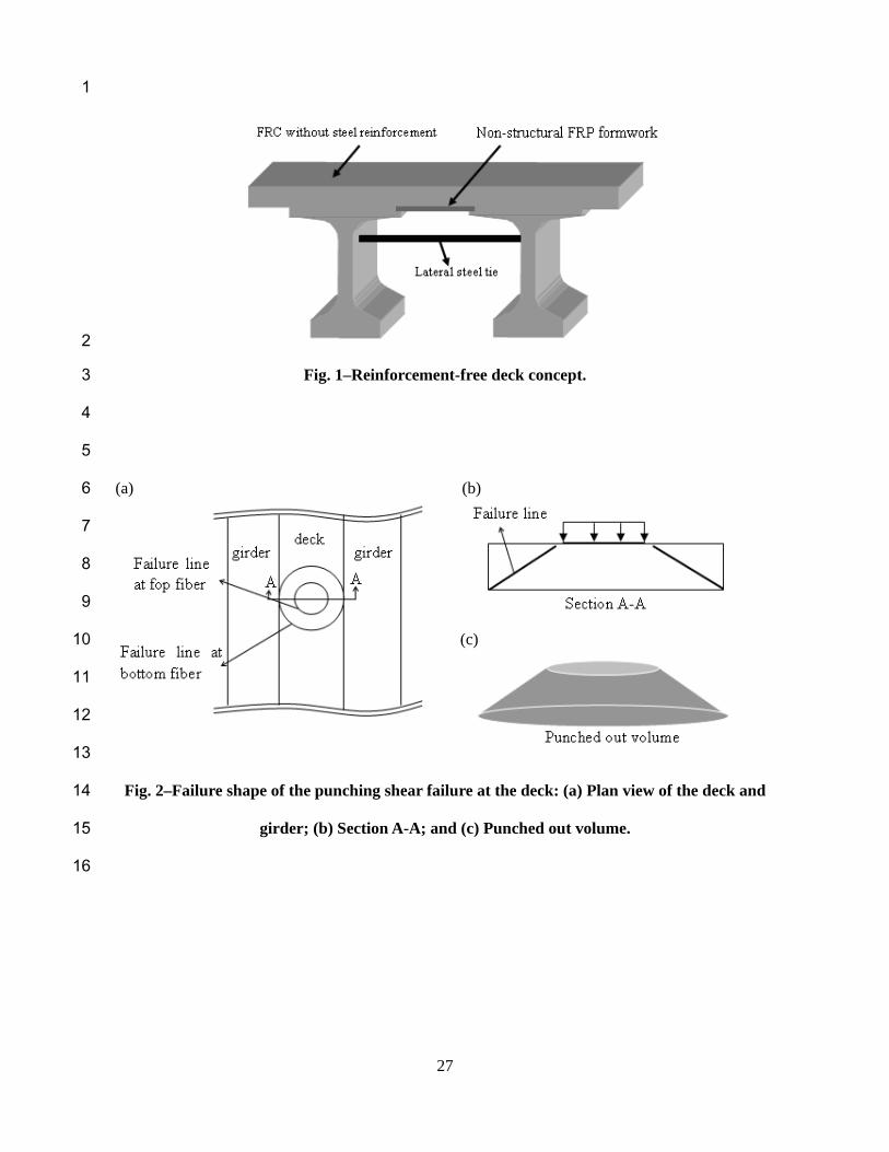
(Fig. 1). Polypropylene fiber, at a volume fraction of 0.32 %, was added to the concrete mix to help 7

control early plastic shrinkage.13 Laboratory experiments14 indicated that the deck had sufficient 8

service and ultimate capacities to resist vehicular loads, without flexural reinforcing, leading to 9

construction of the prototype bridge on a U.S. Highway.12 10

In this paper, a modified STM is developed to predict the strength of this type of reinforcement-free 11

bridge deck. The existing methods of STM analysis described by ACI 3182 cannot be used directly 12

to analyze this restrained deck since the punching shear failure behavior of the deck occurs in 3 13

dimensions and the existing methods cannot capture the enhancement of the flexural strength as a 14

function of the degree of restraint provided. 15

For special permit trucks, unlike the AASHTO design truck, the wheel loadings may have a 16

different effect on a deck. A strength check (low cycle short term behavior) is, however, possible 17

using the proposed STM without any modification (except for the calculation of the effective 18

flexural strip width of the deck; longitudinal wheel spacing should be used when the spacing is less 19

than the effective width) if the spacings of the wheels are not narrower than the clear deck span. 20

21

RESEARCH SIGNIFICANCE 22

A new method to predict the strength of reinforcement-free bridge decks is presented. Traditional 23

bridge deck analysis and design is based on flexural failure. Since most bridge decks actually fail in 24

punching shear under heavy wheel loading, it is evident that improved strength estimations are 25

needed. The proposed method is capable of capturing punching or flexural failure of the restrained 26

4

bridge deck between girders while previously developed analytical models only capture one of the 1

failure modes. This new model is a practical and effective method to replace time consuming FEM 2

analysis. 3

4

CURRENT DECK DESIGN STRENGTH 5

The American Association of State Highway and Transportation Officials (AASHTO)15 provides 6

guidelines for designing or calculating the strength of bridge decks based on the deck flexural 7

resistance between supporting girders. Tests of decks7,11,14,16,17 have shown that failure actually 8

occurs with punching under wheels at loads of approximately five times the AASHTO design 9

service wheel load (with impact). 10

Coincidentally research on fatigue of concrete decks using moving loads has found that failure can 11

occur after 100 million cycles of load at values as low as 14% of the static ultimate capacity of the 12

deck.18 In other words, if the deck is expected to resist 100 million cycles of moving wheel load the 13

design static capacity should be 700% of the fatigue wheel load. The AASHTO fatigue wheel live 14

load, including dynamic load allowance (15 %) and a fatigue load factor (0.75), is 13.8 kips (61.4 15

kN)15. The fatigue design load would then be equal to 97 kips (431 kN). This is also approximately 16

five times the service wheel load – or the capacity now being achieved with a flexural design 17

approach. The fatigue design load is a governing design load since the AASHTO design strength 18

load used in flexural design, including load factor (1.75), dynamic load allowance (33%) and 19

multiple presence factor (1.2) from AASHTO LRFD15, is 44.7 kips (198.8 kN). To achieve the same 20

fatigue life as attained with the current AASHTO flexural design, the capacity of a deck calculated 21

using the modified STM estimate method described here is regarded as sufficient if it can resist a 97 22

kip (431 kN) vehicle wheel load. 23

24

DESCRIPTION OF MODIFIED STM FOR RESTRAINED CONCRETE DECKS 25

The modified STM proposed here for predicting bridge deck strength differs from standard STM in 26

5

that it provides a 2D axisymmetric representation of the behavior of a restrained 3-D bridge deck 1

and in that it is analyzed using 2nd order methods to include geometric nonlinearity of the deck 2

behavior. A detailed description of the proposed model is provided here. 3

4

Geometrical configuration of the model 5

To solve the model in an axisymmetric configuration, the rectangular loaded area from a vehicle 6

wheel is transformed to an equivalent circle, having diameter D, with the same area9 as the actual 7

wheel contact area - shown in Equation (1). 8

bd

D4

(1) 9

This is acceptable since the punching failure of bridge decks generally occurs with a cone shaped 10

failure surface as shown in Fig. 2, even though the loaded area is close to rectangular.9 11

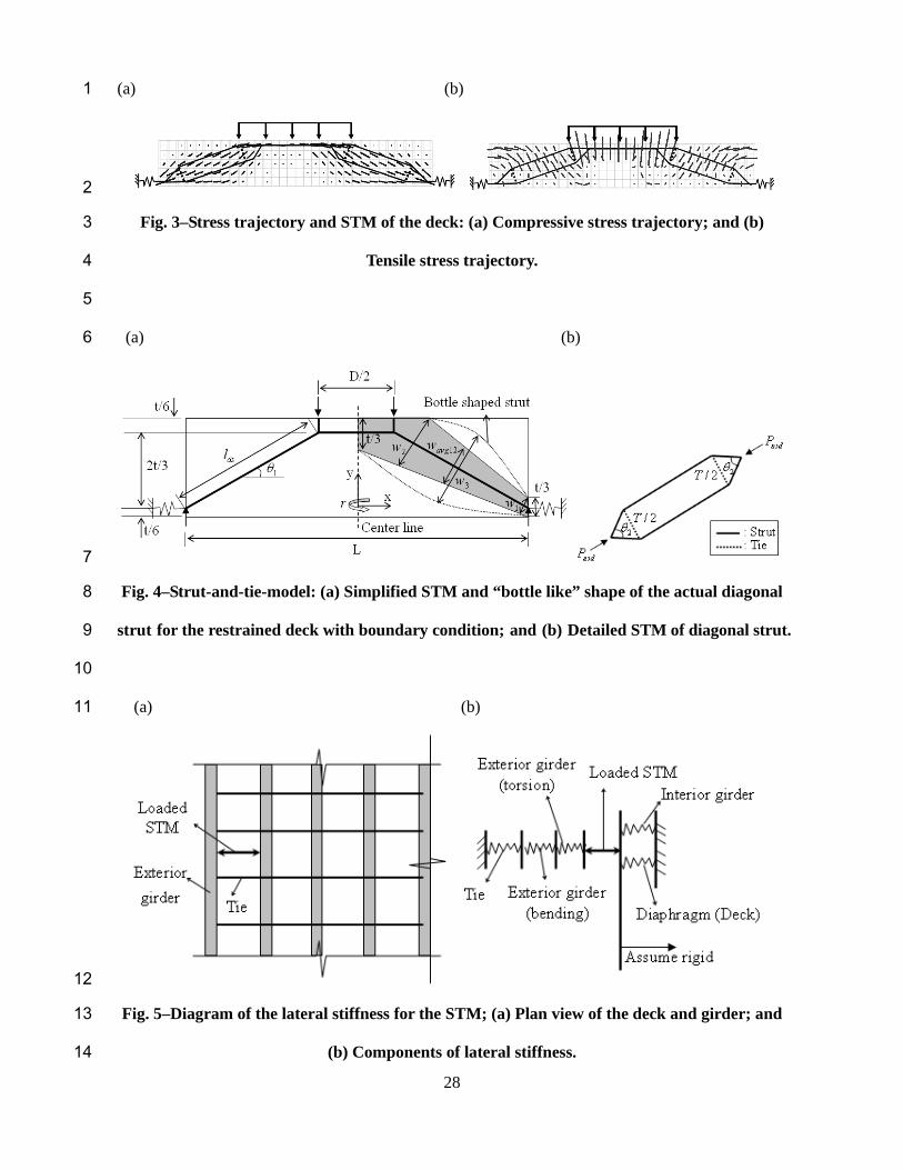
The STM shown in Fig. 3 is constructed assuming that flexural cracking at the negative moment 12

region near the girder has already developed. The compressive and tensile stress trajectories at the 13

failure load level (visible as discrete lines) predicted by a FEM analysis along section A-A of Fig. 2 14

are shown in Fig. 3 and lead to the suggested STM superimposed over the stress lines. The solid 15

lines of the STM represent struts in compression and the dotted lines represent ties (across the 16

struts) in tension. A spring in the lateral direction is placed at the left and right bottom sides of the 17

model, at the deck supports, to simulate axial restraint from adjoining structural elements. 18

The model shown in Fig. 3 is based on an assumption that that the punching failure surface reaches 19

the edge of the girder. From the results of FEM deck modeling, this assumption appears valid for 20

restrained decks thicker than 7 in. (178 mm) with clear deck spans less than 5 ft. (1524 mm). This 21

limitation does not hinder the practical application of the modified STM since the minimum 22

thickness deck prescribed in the AASHTO LRFD bridge design specification15 is 7 in. (178 mm) 23

and the clear deck span in a bridge with wide flange concrete girders rarely exceeds 5 ft. (1524 mm). 24

It is possible to replace the detailed modeling of the diagonal struts shown in Fig. 4(b) with a single 25

6

diagonal strut as shown in Fig. 4(a) as will be described later. The single diagonal strut represents a 1

half portion of the failure surface in Fig. 2(c). The stiffness of the springs at each side of the 2D 2

STM represent the radial outward stiffness caused by restraint from the adjoining slab over a half of 3

the failure line at the bottom fiber shown in Fig. 2(a). 4

Locations for the top and bottom ends of the diagonal strut were determined using a linear bending 5

stress distribution and are shown in Fig. 4(a). The vertical locations of the top lateral strut and the 6

bottom end of the diagonal strut were assumed at the resultants of triangular compressive stress 7

distributions at mid-span where positive moment occurs and near the girder where negative moment 8

occurs, respectively. These placements coincided well with the center of gravity of the compressive 9

stress distribution at these locations predicted from a nonlinear FEM analysis close to the failure 10

load level. 11

The length of the diagonal strut, dsl , and the angle of inclination of the diagonal strut, 1 , can be 12

calculated using the dimensions from Figs. 2 and 4. The average width of the diagonal strut, dsw , 13

that represents the 3-D circumferential surface in the r direction shown in Fig. 4(a) can be 14

calculated as the average of the top and the bottom half circumference of the cone of Fig. 2. 15

L

Dwds 24

(2) 16

It is also necessary to find the width of the diagonal strut for the model in x-y plane (wavg) in Fig. 17

4(a). The width of the diagonal strut at its bottom and its top can be calculated as, 18

11 cos3

tw , 112 cos

3sin

2 tD

w (3) 19

An average width of the diagonal strut (wavg) is taken as the average of the average width of the 20

widths at the two ends and the maximum width of the bottle shaped strut (w3) as shown in Equation 21

(4). The maximum width (w3) of the actual bottle shaped strut shown in Fig. 4(a) must be found 22

from the compressive stress field using a FEM analysis. This analysis has already been completed14 23

for decks on bridges with wide flange concrete girders and the values for w3 can be calculated using 24

7

Table 1. 1

)2

(2

13

21 www

wavg

(4) 2

The average cross-sectional area of the diagonal strut can then be calculated as, 3

dsavgds wwA (5) 4

5

Stiffness of the spring in the model 6

The stiffness of the lateral spring at the supports in the model is a combination of the lateral tie 7

stiffness, the bending stiffness of the girder about its weak axis, the torsional stiffness of the girder, 8

and the in-plane stiffness of the adjoining slab. These components behave like springs in series as 9

shown in Fig. 5 since the deck is restrained by the girders and the girders are restrained by the ties. 10

To be conservative, spring stiffness was just calculated for a deck span adjacent to an external girder 11

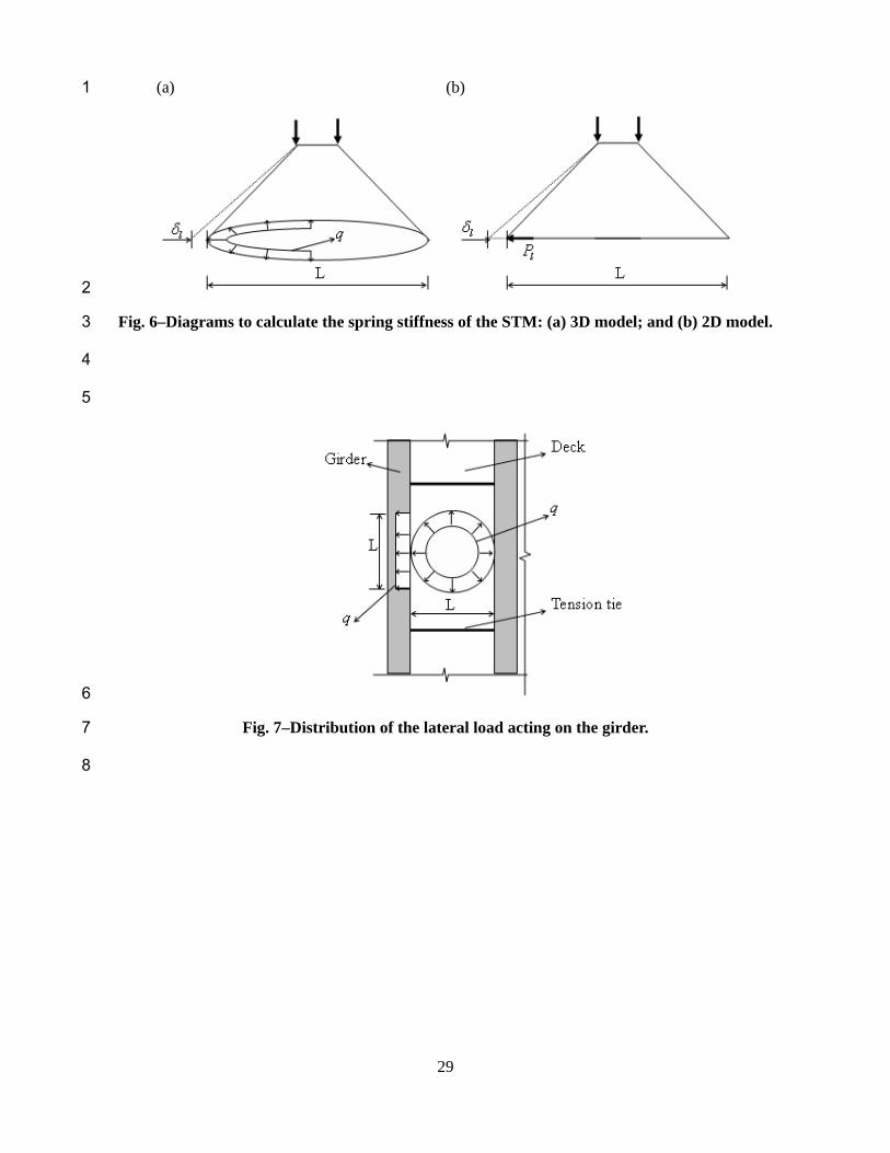
since the lowest lateral restraint occurs at this location. A diagram used to calculate the stiffness of 12

the springs on the exterior side of the 2D STM is shown in Fig. 6. Two approximations are made 13

here: 1) around one half of the bottom of the conical failure surface the restraint is taken as similar 14

to that on the side toward the exterior girder and 2) around the other half the adjacent deck material 15

is assumed to be rigid. The first assumption is judged to be conservative and it appears to be 16

reasonable since the shear failure will start at the location nearest to the exterior girder and then 17

propagate circumferentially. This was found from the observation of the nonlinear FEM analysis, 18

though difficult to see in actual load testing because of the rapid crack growth. The second 19

assumption is made since that side is restrained by a relatively rigid large deck acting as a flat 20

horizontal diaphragm as shown in Fig. 5. 21

The displacement l in Fig. 6 represents the lateral displacement at the bottom left of the exterior 22

strut due to a combination of elongation of the tie, lateral flexural displacement of the girder and 23

torsional rotation of the girder. These deformations are caused by a vertical force which induces a 24

unit distributed load q in the radial direction in the 3D model. The sum of radial outward thrust in 25

8

the form of a single force in the 2D model can be calculated as, 1

LqPl 2

(6) 2

The stiffness of the spring at the bottom left side of the 2D model would be given by Equation (7) 3

using Equation (6) if l were known. 4

ll

ll

LqPK

2 (7) 5

6

Tension tie contribution to spring stiffness: 7

The lateral stiffness provided by the tension ties, ttK , in resisting a single vehicle wheel can be 8

calculated from Equation (8) assuming that the girder is rigid. The tension ties for a particular deck 9

span are anchored on the opposite sides of the girder webs. The length is then Sg, the girder spacing 10

plus the web thickness tw. If the spacing of ties is St, spacing of vehicle axles is Sw, and tie area is At 11

then the stiffness is given as, 12

wwgt

sttt S

tSS

EAK

)( (8) 13

The total transverse lateral force resisted by the ties, due to a single vehicle wheel load, can be 14

calculated as the clear span of the deck (L) times the unit distributed load (q) as shown in Fig. 7. 15

The lateral displacement l due to the elongation of the ties alone can be calculated from the total 16

force divided by the lateral stiffness of the tension ties as, 17

wst

wgt

ttlt SEA

qtSLS

K

qL )(

(9) 18

The stiffness of the spring at the bottom left side of the 2D model, ltK , as contributed by the lateral 19

tension ties is found using Equations (7) and (9) as, 20

wwgt

st

ltlt S

tSS

EALqK

)(22

(10) 21

22

9

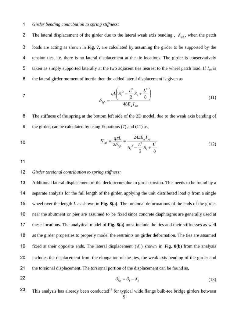
Girder bending contribution to spring stiffness: 1

The lateral displacement of the girder due to the lateral weak axis bending , blg , when the patch 2

loads are acting as shown in Fig. 7, are calculated by assuming the girder to be supported by the 3

tension ties, i.e. there is no lateral displacement at the tie locations. The girder is conservatively 4

taken as simply supported laterally at the two adjacent ties nearest to the wheel patch load. If Iyg is 5

the lateral girder moment of inertia then the added lateral displacement is given as 6

ygg

tt

lgb IE

LS

LSqL

48

82

323

(11) 7

The stiffness of the spring at the bottom left side of the 2D model, due to the weak axis bending of 8

the girder, can be calculated by using Equations (7) and (11) as, 9

82

24

2 323 L

SL

S

IELqK

tt

ygg

lgblgb

(12) 10

11

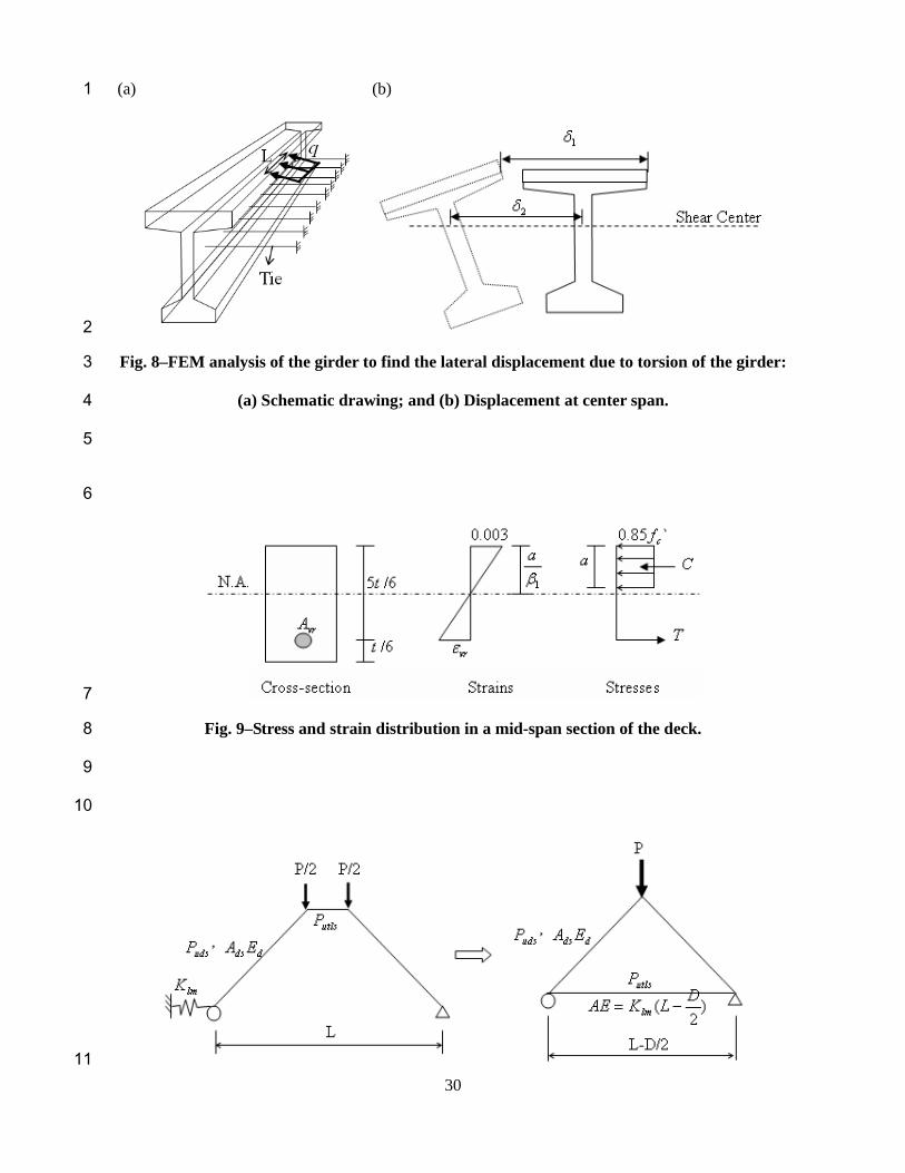
Girder torsional contribution to spring stiffness: 12

Additional lateral displacement of the deck occurs due to girder torsion. This needs to be found by a 13

separate analysis for the full length of the girder, applying the unit distributed load q from a single 14

wheel over the length L as shown in Fig. 8(a). The torsional deformations of the ends of the girder 15

near the abutment or pier are assumed to be fixed since concrete diaphragms are generally used at 16

these locations. The analytical model of Fig. 8(a) must include the ties and their stiffnesses as well 17

as the girder properties to properly model the restraints on girder deformation. The ties are assumed 18

fixed at their opposite ends. The lateral displacement ( 1 ) shown in Fig. 8(b) from the analysis 19

includes the displacement from the elongation of the ties, the weak axis bending of the girder and 20

the torsional displacement. The torsional portion of the displacement can be found as, 21

21 lgt (13) 22

This analysis has already been conducted14 for typical wide flange bulb-tee bridge girders between 23

10

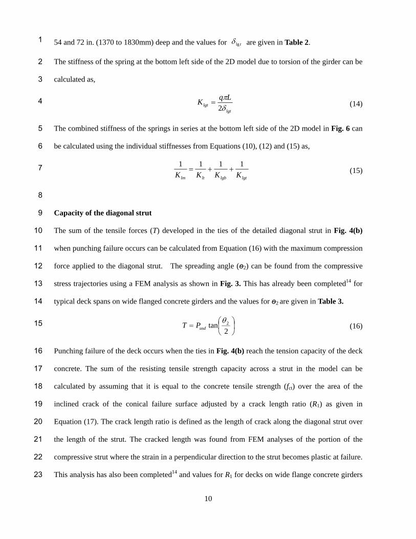
54 and 72 in. (1370 to 1830mm) deep and the values for tlg are given in Table 2. 1

The stiffness of the spring at the bottom left side of the 2D model due to torsion of the girder can be 2

calculated as, 3

lgtlgt

LqK

2 (14) 4

The combined stiffness of the springs in series at the bottom left side of the 2D model in Fig. 6 can 5

be calculated using the individual stiffnesses from Equations (10), (12) and (15) as, 6

lgtlgbltlm KKKK

1111 (15) 7

8

Capacity of the diagonal strut 9

The sum of the tensile forces (T) developed in the ties of the detailed diagonal strut in Fig. 4(b) 10

when punching failure occurs can be calculated from Equation (16) with the maximum compression 11

force applied to the diagonal strut. The spreading angle (ө2) can be found from the compressive 12

stress trajectories using a FEM analysis as shown in Fig. 3. This has already been completed14 for 13

typical deck spans on wide flanged concrete girders and the values for ө2 are given in Table 3. 14

2tan 2

usdPT (16) 15

Punching failure of the deck occurs when the ties in Fig. 4(b) reach the tension capacity of the deck 16

concrete. The sum of the resisting tensile strength capacity across a strut in the model can be 17

calculated by assuming that it is equal to the concrete tensile strength (fct) over the area of the 18

inclined crack of the conical failure surface adjusted by a crack length ratio (R1) as given in 19

Equation (17). The crack length ratio is defined as the length of crack along the diagonal strut over 20

the length of the strut. The cracked length was found from FEM analyses of the portion of the 21

compressive strut where the strain in a perpendicular direction to the strut becomes plastic at failure. 22

This analysis has also been completed14 and values for R1 for decks on wide flange concrete girders 23

11

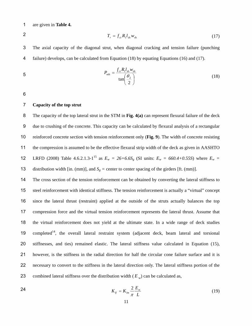
are given in Table 4. 1

dsdsctr wlRfT 1 (17) 2

The axial capacity of the diagonal strut, when diagonal cracking and tension failure (punching 3

failure) develops, can be calculated from Equation (18) by equating Equations (16) and (17). 4

2tan 2

1

dsdsct

uds

wlRfP

(18) 5

6

Capacity of the top strut 7

The capacity of the top lateral strut in the STM in Fig. 4(a) can represent flexural failure of the deck 8

due to crushing of the concrete. This capacity can be calculated by flexural analysis of a rectangular 9

reinforced concrete section with tension reinforcement only (Fig. 9). The width of concrete resisting 10

the compression is assumed to be the effective flexural strip width of the deck as given in AASHTO 11

LRFD (2008) Table 4.6.2.1.3-115 as Ew = 26+6.6Sg (SI units: Ew = 660.4+0.55S) where Ew = 12

distribution width [in. (mm)], and Sg = center to center spacing of the girders [ft. (mm)]. 13

The cross section of the tension reinforcement can be obtained by converting the lateral stiffness to 14

steel reinforcement with identical stiffness. The tension reinforcement is actually a “virtual” concept 15

since the lateral thrust (restraint) applied at the outside of the struts actually balances the top 16

compression force and the virtual tension reinforcement represents the lateral thrust. Assume that 17

the virtual reinforcement does not yield at the ultimate state. In a wide range of deck studies 18

completed14, the overall lateral restraint system (adjacent deck, beam lateral and torsional 19

stiffnesses, and ties) remained elastic. The lateral stiffness value calculated in Equation (15), 20

however, is the stiffness in the radial direction for half the circular cone failure surface and it is 21

necessary to convert to the stiffness in the lateral direction only. The lateral stiffness portion of the 22

combined lateral stiffness over the distribution width ( E w) can be calculated as, 23

L

EKK w

lmlf 2

(19) 24

12

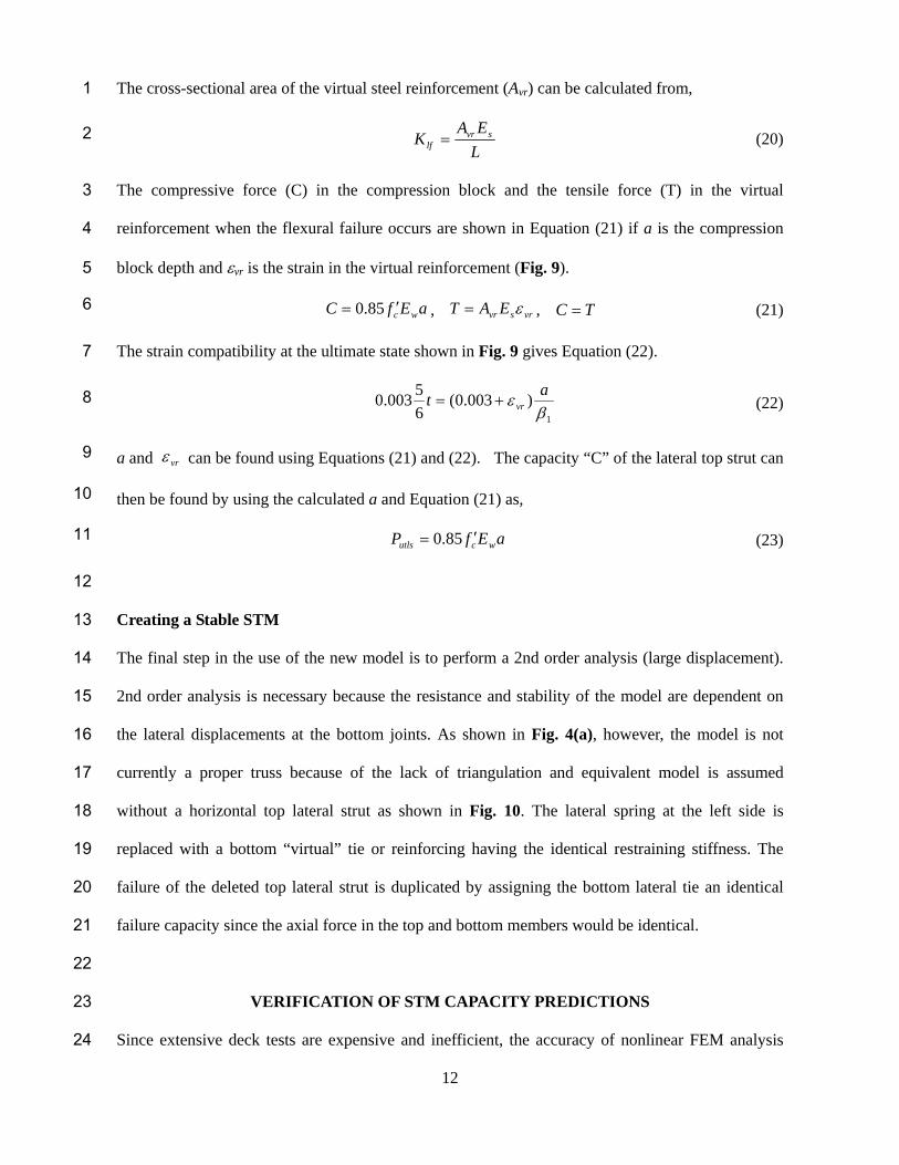
The cross-sectional area of the virtual steel reinforcement (Avr) can be calculated from, 1

L

EAK svr

lf (20) 2

The compressive force (C) in the compression block and the tensile force (T) in the virtual 3

reinforcement when the flexural failure occurs are shown in Equation (21) if a is the compression 4

block depth and vr is the strain in the virtual reinforcement (Fig. 9). 5

aEfC wc 85.0 , vrsvr EAT , TC (21) 6

The strain compatibility at the ultimate state shown in Fig. 9 gives Equation (22). 7

1

)003.0(6

5003.0

a

t vr (22) 8

a and vr can be found using Equations (21) and (22). The capacity “C” of the lateral top strut can 9

then be found by using the calculated a and Equation (21) as, 10

aEfP wcutls 85.0 (23) 11

12

Creating a Stable STM 13

The final step in the use of the new model is to perform a 2nd order analysis (large displacement). 14

2nd order analysis is necessary because the resistance and stability of the model are dependent on 15

the lateral displacements at the bottom joints. As shown in Fig. 4(a), however, the model is not 16

currently a proper truss because of the lack of triangulation and equivalent model is assumed 17

without a horizontal top lateral strut as shown in Fig. 10. The lateral spring at the left side is 18

replaced with a bottom “virtual” tie or reinforcing having the identical restraining stiffness. The 19

failure of the deleted top lateral strut is duplicated by assigning the bottom lateral tie an identical 20

failure capacity since the axial force in the top and bottom members would be identical. 21

22

VERIFICATION OF STM CAPACITY PREDICTIONS 23

Since extensive deck tests are expensive and inefficient, the accuracy of nonlinear FEM analysis 24

13

strength prediction for a large series of deck configurations was used as a basis of comparison with 1

the STM strength predictions. ABAQUS19 was used to conduct the FEM analyses. A complete 2

description of the FEM analysis technique is provided elsewhere14, 20. Validation of the FEM 3

analysis method strength prediction capability was achieved by comparison with a restrained deck 4

element experimental test as shown in Fig. 11. 14, 20 The strength prediction error was 6%, an 5

acceptable amount for estimating capacity of a structure that is very non-linear with a non-6

homogenous material. 7

A parametric study on the ultimate capacity of bridge decks using both FEM analysis and the 8

modified STM were performed to verify the STM predictions and to identify key performance 9

characteristics affected by design parameters. Ninety four analyses were conducted with variations 10

in deck depth, span, concrete strength, girder type and size, and restraint provided by ties between 11

Wisconsin 54 inch (1372 mm) deep girders21. 12

A deck restraing factor “R” given in Equation (24) was derived to describe the restraint provided by 13

steel ties between the girders. 14

)()(

)()(

tiessteellateralofspacinggirdersofspacingcentertocenter

deckofthicknesstiesteellateralaofstiffnessaxialR

(24) 15

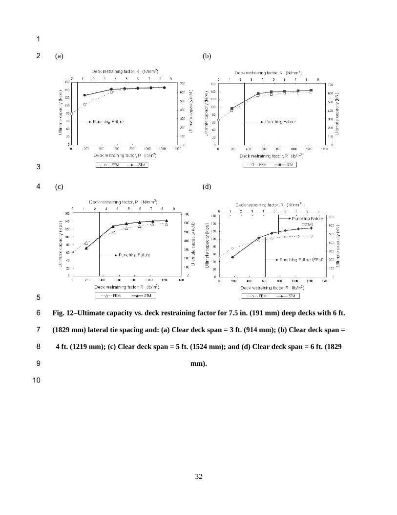
The results for a 7.5 in. (191 mm) deep deck with a 6 ft. (1829 mm) lateral tie spacing are shown in 16

Fig. 12. The comparison of the FEM and STM methods shows generally acceptable agreement, i.e. 17

small error, for clear deck spans less than 6 ft. (1830mm). When the clear deck span was 6 ft. (1830 18

mm) the STM analysis showed 4 ~ 18 % higher capacity compared to the FEM analysis. These 19

results indicate the STM may be unsafe for long span deck capacity and the application should be 20

limited to normal deck spans. 21

The failure mode changes from flexural to punching shear if an appropriate level of restraint exists. 22

The required amount of restraint appears to depend on the deck span length. Shear failure generally 23

occurred when the restraint (R) was above 600 lb/in2 (4.13 N/mm2). Improvement in the ultimate 24

strength is minimal with an increase of the deck restraining factor ( R ) over 900 lb/in2 (6.20 25

14

N/mm2). It is, therefore, recommended to design the lateral steel tie to provide the deck with a 1

restraining factor ( R ) of at least 900 lb/in2 (6.20 N/mm2). 2

FEM and STM analyses for a 7.5 in. (191 mm) deep deck with 8 ft. and 10ft. (2438 mm or 3050 3

mm) lateral tie spacings were also performed. The results were similar to those shown in Fig. 12. 4

The results indicate that for a given span length, deck thickness and deck restraining factor, the 5

failure capacity does not change significantly with tie spacings between 6ft. and 10ft. (1830 mm 6

and 3050 mm). Additional FEM and STM analyses were performed for two other types of wide 7

flange girders, Wisconsin 72W girders and Washington state WS53 girders, and the comparison 8

showed generally acceptable agreement14, 20. 9

10

SIMPLIFIED CAPACITY EQUATION 11

An alternate simpler method to predict the ultimate capacity of reinforcement-free decks on 54 to 12

72 in. (1372 to 1829 mm) deep wide flanged precast girders, for a wheel having an AASHTO15 13

patch size, is given by Pd as, 14

225.0

541.0894.113

td

tdddd S

KLtP (SI units:

225.0

541.0894.1227.2

td

tdddd S

KLtP ) (25) 15

The equation was fitted to results from the FEM parametric analyses. Restraint factors (R) of 200 16

lb/in2 to 1200 lb/in2 (1.38 N/mm2 to 8.27 N/mm2) were used with clear spans of 3 ft to 6 ft. (914 17

mm to 1829 mm), deck thicknesses of 7.0 in. to 9.0 in. (178 mm to 229mm) deck thickness, and 18

lateral steel tie spacing of 6 ft. to 10 ft. (1829 mm to 3048 mm). 19

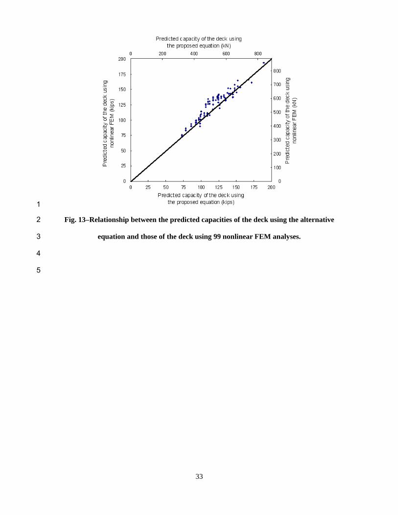
The equation on average predicted 94.8 % of the deck capacity defined by FEM analysis results. 20

The standard deviation was 5.8 %. The relationship between the predicted capacities of the deck 21

using the proposed equation and those of the deck using nonlinear FEM analysis is shown in Fig. 13. 22

The bold line in Fig. 13 indicates the result if the two analyses matched perfectly. Most of the points 23

are at the upper side of the bold line indicating that the proposed equation is conservative. 24

25

15

STM CAPACITY CALCULATION EXAMPLE 1

A step by step capacity calculation example for a reinforcement-free deck on 54 in. (1372mm) deep 2

wide flanged girders using the developed equations and the alternative equation is illustrated here. 3

1) Given information for the sample deck on Wisconsin 54W girders when the clear span of the 4

deck between girders is known: 5

Clear span of the deck: L = 4ft. (1219 mm) 6

Spacing of the girders: Sg = 8ft. (2438 mm) 7

Thickness of the web of the girder: tw = 6.5 in. (165 mm) 8

Design compressive strength of the deck: fc’ = 4000 psi (27.6 MPa), 1 =0.85 9

Design compressive strength of the girder: fc’ = 8000 psi (55.1 MPa) 10

Modulus of elasticity of the deck: Ed = 3605 ksi (24.8 GPa) 11

Modulus of elasticity of the girder: Eg = 5098 ksi (35.1 GPa) 12

Moment of inertia of the girder in weak axis: Iyg = 125056 in.4 (52,052106 mm4) 13

Modulus of elasticity of the lateral steel tie: Es = 29,000 ksi (199.8 GPa) 14

Spacing of the vehicle axles in longitudinal direction: Sw = 14 ft. (4267 mm) 15

Depth of the deck: t = 7.5 in. (191 mm) 16

Spacing of lateral steel ties: St = 10 ft. (3048 mm) 17

2) Find the needed axial stiffness of a single lateral tie ( tK ) from Equation (24) using the 18

recommended deck restraining factor (R) = 900 lb/in2. (6.20 N/mm2) 19

Kt = (900 lb/in2) Sg St / t = 1382.4 kip/in (242.1 kN/mm) 20

3) Calculate the cross-sectional area of a single lateral tie from the axial stiffness found above. 21

tK = )( wg

st

tS

EA

,

s

wgtt E

tSKA

)( = 4.886 in.2 (3152 mm2) 22

Assume tension tie bars with 2.5 in. (64 mm) diameter. 23

4

)7.2( 2inAt

= 4.909 in.2 (3167 mm2) 24

16

4) Find parameters from Tables 1-4. 1

2 = 53.117°, R2 = 1.50, 1R = 0.565, tlg = 0.0257 in. (0.653 mm) 2

5) Predict the ultimate capacity of the deck system using the modified STM analysis. 3

Calculate cross-sectional area of the diagonal strut using Equations (1)-(5). 4

1 =14.03°, lds = 20.63 in. (524.00 mm), D = 15.96 in. (405.38 mm), wds = 43.97 in. (1116.73 mm), 5

w1 = 2.43 in. (61.61 mm), w2 = 4.36 in. (110.73 mm), wavg = 6.79 in. (172.34 mm), 6

dsA = 298.31 in.2 (192,457.40 mm2) 7

Calculate combined restraint lmK using Equations (10), (12), (13) and (15) 8

ltK = 3,054,324 lb/in. (534,867 N/mm), bK lg = 29,977,388 lb/in. (5,249,583 N/mm) 9

tK lg = 2,933,783 lb/in (513,759 N/mm), lmK = 1,425,273 lb/in. (249,591 N/mm) 10

Calculate capacity of the truss members using Equations (18)-(23) 11

udsP 324,087 lb (1,441,541 N), SEw 6.626 = 78.8 in. (2001 mm), vrA = 2.446 in.2 (mm2), 12

a = 1.701 in. (43.21 mm), utlsP = 455,604 lb (2,026,527 N) 13

Construct the modified STM and perform 2nd order (P-delta) analysis to check if the model has 14

sufficient capacity to withstand the design load [97 kips (431 kN)]. 15

The member forces of the model under the design load were 218.4 kips (971 kN) for the diagonal 16

member and 231.6 kips (1030 kN) for the lateral member, indicating that the section of the deck 17

system is safe. 18

The ultimate capacity found from the second order truss analysis was 141.3 kips (629 kN). The 19

member forces at the failure of the model were 324.1 kips (1442 kN) for the diagonal member and 20

318.0 kips (1414 kN) for the lateral member. The diagonal member reached its capacity first - 21

indicating that the failure mode was a punching failure. 22

6) Comparison with the result using the proposed equation alternative to the modified STM analysis. 23

Use Equation (25) to calculate the predicted capacity of the deck. 24

td = 7.5 in. (191 mm), Ld = 4ft. = 48 in. (1219 mm), 25

17

tdK = )( wg

st

tS

EA

= 1389 kip/in (243.2 kN/mm), Std = 10 ft. = 120 in. (3048 mm), 1

225.0

541.0894.113

td

tdddd S

KLtP = 126.2 kips (561 kN) 2

The predicted capacity using the alternative equation is 126.2 kips (561 kN) versus the predicted 3

capacity using the modified STM [141.3 kips (629 kN)]. 4

5

CONCLUSIONS 6

The following conclusions may be made based on the development process of a new analysis tool 7

for the reinforcement free-decks: 8

1 The design load for reinforcement-free bridge decks on concrete wide flange girders was 9

examined based on the current AASHTO specification and previous studies on the capacity 10

of concrete decks under moving vehicle loads. The controlling state is the fatigue limit state 11

requiring a strength design load of 97 kips (431 kN) for a vehicle wheel load. This is a much 12

more severe design load than used in present design methods and specifications, but the 13

capacities of the restrained deck are also higher than expected. 14

2 The proposed equivalent 2D strut-and-tie model (STM) can effectively replace a time 15

consuming FEM analysis for predicting the capacity of a 7 in. (178 mm) or thicker [to 12 in. 16

(305mm)] restrained deck on concrete wide flange girders when the deck clear span does not 17

exceed 5 ft. (1524 mm) if the parameters predefined in Tables 1-4 are used. This limitation 18

does not hinder the practical application of the modified STM for the reinforcement-free 19

deck system since the minimum thickness of the deck prescribed in AASHTO LRFD bridge 20

design specification15 is 7 in. (178 mm) and the clear deck span of concrete wide flange 21

girder bridges rarely exceeds 5 ft. (1524 mm). 22

18

3 The model is capable of capturing the punching shear failure and the failure at mid-span due 1

to flexural crushing of concrete. The model provides an acceptable 2D axisymmetric 2

representation of the behavior of the restrained 3D deck. 3

4 The predicted capacities using the STM analyses for a 7.5 in. (191 mm) deep deck are 4

acceptable when the clear deck spans were between 3 ft. and 5 ft. (914 mm and 1524 mm). 5

When the clear deck span was 6 ft. (1829 mm) the STM analysis showed 4 ~ 18% higher 6

capacity compared to the FEM analysis. This result indicates that the proposed method 7

should currently be limited to deck clear spans of 5 ft. (1524 mm) or less. 8

5 The proposed method may be used for steel girders with clear deck spacing of less than 5 ft. 9

(1524 mm). In order to apply the method to steel girders it is necessary to evaluate the 10

contribution of the steel girders to the lateral stiffness of the restraining system. 11

12

ACKNOWLEDGEMENT 13

This project was supported through funding provided by the Federal Highway Administration 14

through the Wisconsin Department of Transportation under the Innovative Bridge Research and 15

Construction program. 16

17

NOTATION 18

a = height of a Whitney equivalent rectangular compressive stress block 19

dsA = average cross-sectional area of the diagonal strut 20

tA = cross-sectional area of a single steel tension tie 21

b = lateral (in perpendicular direction to the girder) length of the rectangular loading area 22

d = longitudinal (in parallel direction to the girder) length of the rectangular loading area 23

D = diameter of equivalent circular loading area 24

gE = elastic modulus of the girder 25

19

sE = modulus of elasticity of steel 1

ctf = tensile strength of the deck given by cf 5 psi (0.415 cf MPa), cf in psi (MPa) 2

ygI = weak axis moment of inertia of the girder 3

lK = stiffness of the spring at the bottom left side of the 2D model 4

lfK = lateral portion of the combined lateral stiffness 5

lgbK = stiffness of the spring at the bottom left side of the 2D model due to weak axis bending of 6

the girder 7

lgtK = stiffness of the spring at the bottom left side of the 2D model due to torsion of the girder 8

lmK = stiffness of the spring at the bottom left side of the 2D model 9

ltK = stiffness of the spring at the bottom left side of the 2D model representing the lateral 10

tension tie contribution to the restraint 11

tdK = axial stiffness of single lateral tie in Equation (25) [=)( wg

st

tS

EA

, kips/in (kN/mm)] 12

ttK = lateral stiffness of the tension ties resisting a single vehicle wheel 13

dsl = length of the diagonal strut 14

L = deck clear span between girder flanges 15

Ld = deck clear span between girder flanges in Equation (25), in. (mm) 16

dP = wheel load capacity of the deck in Equation (25), kips (kN) 17

lP = a sum of radial outward thrust in the form of a single force in the 2D model 18

usdP = capacity of the diagonal strut 19

utlsP = capacity of the lateral top strut 20

20

q = unit distributed thrust around the 3D cone 1

R = deck restraining factor 2

1R = a ratio of (cracked length found from FEM)/ dsl 3

tS = spacing of the tension ties 4

tdS = spacing of the tension ties in Equation (25), in. (mm) 5

gS = center to center spacing of the girders 6

wS = spacing of the vehicle axle in a longitudinal (parallel direction to the girder) direction 7

t = deck thickness 8

td = deck thickness in Equation (25), in. (mm) 9

wt = thickness of the web of the girder 10

T = sum of tensile force in the ties 11

rT = sum of resisting capacity of the ties 12

12avgw = average width of 1w and 2w 13

dsw = width of diagonal strut around half the circumference of the failure cone, in r direction 14

1w = width of the diagonal strut at its bottom 15

2w = width of the diagonal strut at its top 16

1 = a factor relating the depth of equivalent rectangular compressive stress block to the 17

neutral axis depth 18

l = lateral displacement in the STM due to the elongation of the restraints 19

lgb = lateral displacement due to bending of the girder in its weak axis 20

lgt = lateral torsional displacement at the top of the girder 21

lt = lateral displacement in STM due to the elongation of the tie 22

1 = lateral displacement at the loading location 23

21

2 = lateral displacement at the shear center of the girder 1

vr = strain in the virtual reinforcement 2

1 = angle of inclination of the diagonal strut 3

2 = spreading angle of the compressive force 4

5

REFERENCES 6

1. Schlaich, J.; Schafer, K.; and Jennewein, M., “Towards a Consistent Design of Structural 7

Concrete,” Journal of the Prestressed Concrete Institute, V. 32, 1978, pp. 74-150. 8

2. ACI Committee 318, “Building Code Requirements for Structural Concrete (ACI 318-08) and 9

Commentary (318R-08),” American Concrete Institute, Farmington Hills, MI, USA, 2008. 10

3. Tan, K. H., “Size Effect on Shear Strength of Deep Beams: Investigating with Strut-and-Tie 11

Model,” Journal of the Structural Engineering, ASCE, V. 132, No. 5, 2006, pp. 673-685. 12

4. Brena, S. F., and Morrison, M. C., “Factors Affecting Strength of Elements Designed using Strut-13

and-Tie Models,” ACI Structural Journal, V.104, No. 3, 2007, pp. 267-277. 14

5. Ley, M. T.; Riding, K. A.; Widianto.; Bae, S.; and Breen, J. E., “Experimental Verification of 15

Strut-and-Tie Model Design Method,” ACI Structural Journal, V. 104, No. 6, 2007, pp. 749-755. 16

6. Park, J., and Kuchma, D., “Strut-and-tie Model Analysis for Strength Prediction of Deep Beams,” 17

ACI Structural Journal, V. 104, No. 6, 2007, pp. 657-666. 18

7. Hewitt, B. E,. and Batchelor, B. deV., “Punching Shear Strength of Restrained Slabs,” Journal of 19

Structural Division, ASCE, V. 101, No. ST9, 1975, pp. 1837-1853. 20

8. Kuang, J. S., and Moley, C. T., “A Plasticity Model for Punching Shear of Laterally Restrained 21

Slabs with Compressive Membrane Action,” International Journal of Mechanical Sciences, V. 32, 22

No. 5, 1993, pp. 371-385. 23

9. Mufti, A. A., and Newhook, J. P., “Punching Shear Strength of Restrained Concrete Bridge Deck 24

Slabs,” ACI structural journal, V. 95, No. 4, 1998, pp. 375-381. 25

22

10. Mufti, A. A.; Bakht, B.; and Jaeger, L. G., “Fiber FRC Deck Slabs with Diminished Steel 1

Reinforcement,” IABSE Symposium Proceedings (Leningrad), 1991, pp. 388-389. 2

11. Mufti, A. A.; Jaeger, L. G..; Bakht, B.; and Wegner, L. D., “Experimental Investigation of Fibre-3

reinforced Concrete Deck Slabs without Internal Steel Reinforcement,” Canadian Journal of Civil 4

Engineering, V. 20, No. 3, Jun, 1993, pp. 398-406. 5

12. Oliva, M. G..; Bae, H.; Bank, L. C.; Russell, J. S.; Carter, J. W.; and Becker, S., “Design and 6

Construction of a Reinforcement Free Concrete Bridge Deck on Precast Bulb Tee Girders,” 7

Proceedings 2007 PCI/FHWA National Bridge Conference, Phoenix, AZ, USA, October 21-24, 8

2007, CD-ROM. 9

13. Naaman, A. E.; Wongtanakitcharoen; T.; and Hauser, G., “Influence of Different Fibers on 10

Plastic Shrinkage Cracking of Concrete,” ACI Materials Journal, V. 102, No. 1, 2005, pp. 49-58. 11

14. Bae, H., “Design of Reinforcement-free Bridge Decks with Wide Flange Prestressed Precast 12

Girders,” PhD Thesis, University of Wisconsin, Madison, WI, USA, 2008. 13

15. AASHTO., AASHTO LRFD Bridge Design Specifications, 4th Ed., American Association of 14

State Highway and Transportation Officials, Washington, D.C., 2008. 15

16. Dieter, D. A.; Dietsche, J. S.; Bank, L. C.; Oliva, M. G.; and Russell, J. S., “Concrete Bridge 16

Decks Constructed with FRP Stay-in-Place Forms and FRP Grid Reinforcing,” Journal of the 17

Transportation Research Board 1814, TRB, National Research Council, Washington, D.C., 2002, 18

pp. 219-226. 19

17. Bank, L. C.; Oliva, M. G.; Russell, J. S.; Jacobson, D. A., Conachen, M.; Nelson, B.; and 20

McMonigal, D., “Double Layer Prefabricated FRP Grids for Rapid Bridge Deck Construction: Case 21

Study,” Journal of Composites for Construction, ASCE, V. 10, No. 3, 2006, pp. 204-221. 22

18. Petrou, M. F.; Perdikaris, P. C.; and Wang, A., “Fatigue Behavior of Noncomposite Reinforced 23

Concrete Bridge Deck Models,” Transportation Research Board 1460, TRB, National Research 24

Council, Washington, D.C., 1994, pp. 73-80. 25

19. Hibbitt, Karlsson & Sorensen Inc., “ABAQUS User’s manual,” Hibbitt, Karlsson & Sorensen 26

23

Inc., Pawtucket, RI, USA, 2004. 1

20. Bae, H.; Oliva, M. G.; and Bank, L. C., “Obtaining optimal performance with reinforcement-2

free concrete highway bridge decks,” Engineering Structures, V. 32, No. 8, 2010, pp. 2300-2309. 3

21. Wisconsin Department of Transportation., WisDOT Bridge Manual, Wisconsin Department of 4

Transportation, Madison, WI, USA, 2010. (Website: http://www.dot.wisconsin.gov) 5

6

TABLES and FIGURES 7

8

List of Tables: 9

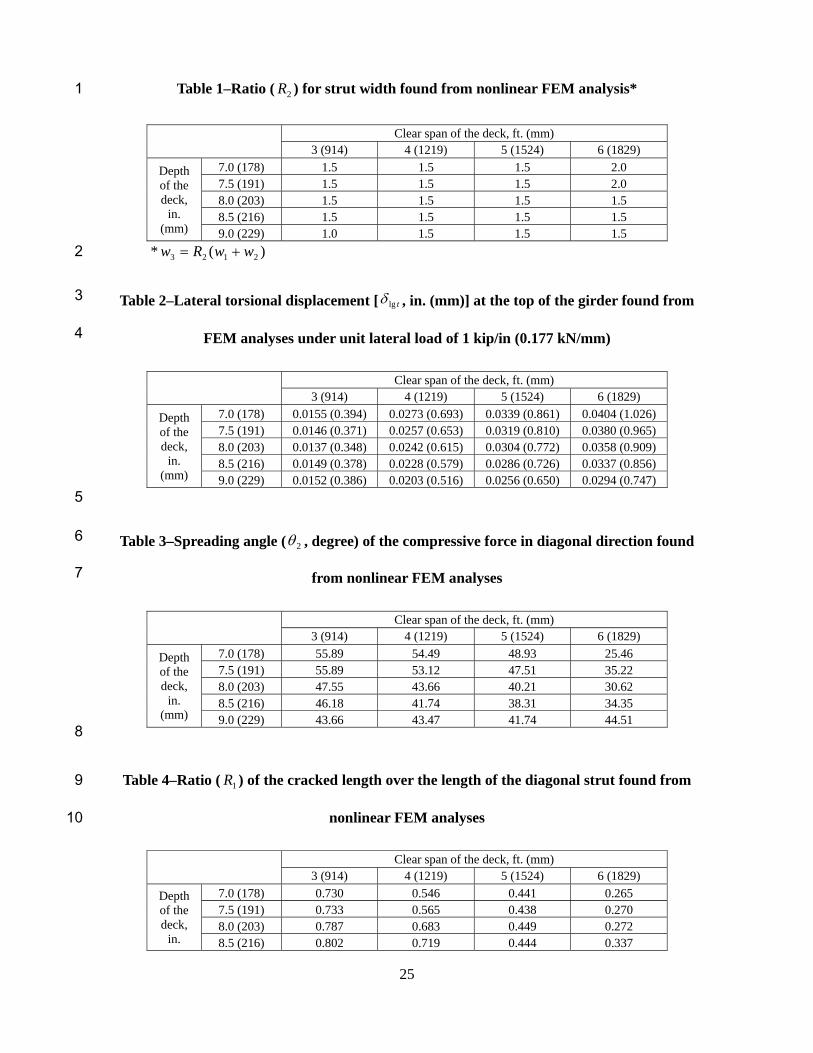
Table 1 – Ratio ( 2R ) for strut width found from nonlinear FEM analysis 10

Table 2 – Lateral torsional displacement [ tlg , in. (mm)] at the top of the girder found from FEM 11

analyses under unit lateral load of 1 kip/in (0.177 kN/mm) 12

Table 3 – Spreading angle ( 2 , degree) of the compressive force in diagonal direction found from 13

nonlinear FEM analyses 14

Table 4 – Ratio ( 1R ) of the cracked length over the length of the diagonal strut found from 15

nonlinear FEM analyses 16

17

List of Figures: 18

Fig. 1 – Reinforcement-free deck concept. 19

Fig. 2 – Failure shape of the punching shear failure at the deck: (a) Plan view of the deck and 20

girder; (b) Section A-A; and (c) Punched out volume 21

Fig. 3 – Stress trajectory and STM of the deck: (a) Compressive stress trajectory; and (b) Tensile 22

stress trajectory. 23

Fig. 4 – Strut-and-tie-model: (a) Simplified STM and “bottle like” shape of the actual diagonal strut 24

for the restrained deck with boundary condition; and (b) Detailed STM of diagonal strut. 25

24

Fig. 5 – Diagram of the lateral stiffness for the STM; (a) Plan view of the deck and girder; and (b) 1

Components of lateral stiffness. 2

Fig. 6 – Diagrams to calculate the spring stiffness of the STM: (a) 3D model; and (b) 2D model. 3

Fig. 7 – Distribution of the lateral load acting on the girder. 4

Fig. 8 – FEM analysis of the girder to find the lateral displacement due to torsion of the girder: (a) 5

Schematic drawing; and (b) Displacement at center span. 6

Fig. 9 – Stress and strain distribution in a mid-span section of the deck. 7

Fig. 10 – Simplification of the STM (Ed is modulus of elasticity of the deck). 8

Fig. 11 – Load vs. displacement plots from FEM analyses and restrained deck element experiment. 9

Fig. 12 – Ultimate capacity vs. deck restraining factor for 7.5 in. (191 mm) deep decks with 6 ft. 10

(1829 mm) lateral tie spacing and: (a) Clear deck span = 3 ft. (914 mm); (b) Clear deck span = 4 ft. 11

(1219 mm); (c) Clear deck span = 5 ft. (1524 mm); and (d) Clear deck span = 6 ft. (1829 mm). 12

Fig. 13 – Relationship between the predicted capacities of the deck using the alternative equation 13

and those of the deck using 99 nonlinear FEM analyses. 14

15

25

Table 1–Ratio ( 2R ) for strut width found from nonlinear FEM analysis* 1

Clear span of the deck, ft. (mm)

3 (914) 4 (1219) 5 (1524) 6 (1829)

Depth of the deck,

in. (mm)

7.0 (178) 1.5 1.5 1.5 2.0 7.5 (191) 1.5 1.5 1.5 2.0 8.0 (203) 1.5 1.5 1.5 1.5 8.5 (216) 1.5 1.5 1.5 1.5 9.0 (229) 1.0 1.5 1.5 1.5

* )( 2123 wwRw 2

Table 2–Lateral torsional displacement [ tlg , in. (mm)] at the top of the girder found from 3

FEM analyses under unit lateral load of 1 kip/in (0.177 kN/mm) 4

Clear span of the deck, ft. (mm)

3 (914) 4 (1219) 5 (1524) 6 (1829)

Depth of the deck,

in. (mm)

7.0 (178) 0.0155 (0.394) 0.0273 (0.693) 0.0339 (0.861) 0.0404 (1.026) 7.5 (191) 0.0146 (0.371) 0.0257 (0.653) 0.0319 (0.810) 0.0380 (0.965) 8.0 (203) 0.0137 (0.348) 0.0242 (0.615) 0.0304 (0.772) 0.0358 (0.909) 8.5 (216) 0.0149 (0.378) 0.0228 (0.579) 0.0286 (0.726) 0.0337 (0.856) 9.0 (229) 0.0152 (0.386) 0.0203 (0.516) 0.0256 (0.650) 0.0294 (0.747)

5

Table 3–Spreading angle ( 2 , degree) of the compressive force in diagonal direction found 6

from nonlinear FEM analyses 7

Clear span of the deck, ft. (mm)

3 (914) 4 (1219) 5 (1524) 6 (1829)

Depth of the deck,

in. (mm)

7.0 (178) 55.89 54.49 48.93 25.46 7.5 (191) 55.89 53.12 47.51 35.22 8.0 (203) 47.55 43.66 40.21 30.62 8.5 (216) 46.18 41.74 38.31 34.35 9.0 (229) 43.66 43.47 41.74 44.51

8

Table 4–Ratio ( 1R ) of the cracked length over the length of the diagonal strut found from 9

nonlinear FEM analyses 10

Clear span of the deck, ft. (mm)

3 (914) 4 (1219) 5 (1524) 6 (1829)

Depth of the deck,

in.

7.0 (178) 0.730 0.546 0.441 0.265 7.5 (191) 0.733 0.565 0.438 0.270 8.0 (203) 0.787 0.683 0.449 0.272 8.5 (216) 0.802 0.719 0.444 0.337

26

(mm) 9.0 (229) 0.891 0.719 0.444 0.335

1

27

1

2

Fig. 1–Reinforcement-free deck concept. 3

4

5

(a) (b) 6

7

8

9

(c) 10

11

12

13

Fig. 2–Failure shape of the punching shear failure at the deck: (a) Plan view of the deck and 14

girder; (b) Section A-A; and (c) Punched out volume. 15

16

28

(a) (b) 1

2

Fig. 3–Stress trajectory and STM of the deck: (a) Compressive stress trajectory; and (b) 3

Tensile stress trajectory. 4

5

(a) (b) 6

7

Fig. 4–Strut-and-tie-model: (a) Simplified STM and “bottle like” shape of the actual diagonal 8

strut for the restrained deck with boundary condition; and (b) Detailed STM of diagonal strut. 9

10

(a) (b) 11

12

Fig. 5–Diagram of the lateral stiffness for the STM; (a) Plan view of the deck and girder; and 13

(b) Components of lateral stiffness. 14

29

(a) (b) 1

2

Fig. 6–Diagrams to calculate the spring stiffness of the STM: (a) 3D model; and (b) 2D model. 3

4

5

6

Fig. 7–Distribution of the lateral load acting on the girder. 7

8

30

(a) (b) 1

2

Fig. 8–FEM analysis of the girder to find the lateral displacement due to torsion of the girder: 3

(a) Schematic drawing; and (b) Displacement at center span. 4

5

6

7

Fig. 9–Stress and strain distribution in a mid-span section of the deck. 8

9

10

11

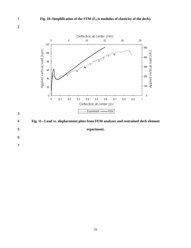
31

Fig. 10–Simplification of the STM (Ed is modulus of elasticity of the deck). 1

2

3

Fig. 11– Load vs. displacement plots from FEM analyses and restrained deck element 4

experiment. 5

6

7

32

1

(a) (b) 2

3

(c) (d) 4

5

Fig. 12–Ultimate capacity vs. deck restraining factor for 7.5 in. (191 mm) deep decks with 6 ft. 6

(1829 mm) lateral tie spacing and: (a) Clear deck span = 3 ft. (914 mm); (b) Clear deck span = 7

4 ft. (1219 mm); (c) Clear deck span = 5 ft. (1524 mm); and (d) Clear deck span = 6 ft. (1829 8

mm). 9

10

33

1

Fig. 13–Relationship between the predicted capacities of the deck using the alternative 2

equation and those of the deck using 99 nonlinear FEM analyses. 3

4

5