Embed Size (px)
Citation preview
Two-Parameter Selection Techniques forProjection-based Regularization Methods:
Application to Partial-Fourier pMRI
Misha E. Kilmer1
Scott Hoge2
1 Dept. of Mathematics, Tufts UniversityMedford, MA
2 Dept. of Radiology, Brigham and Women’s Hospital andHarvard Medical School, Boston, MA
Two-Parameter Selection Techniques for Projection-based Regularization Methods – p. 1/29
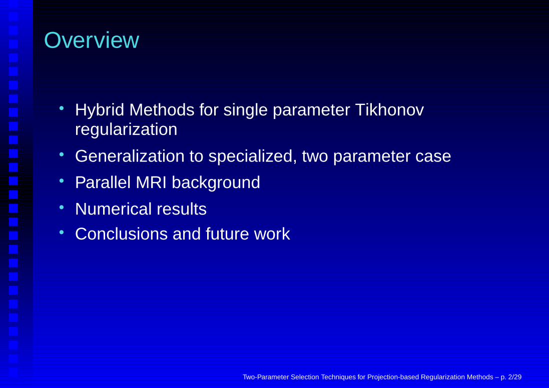
Overview
• Hybrid Methods for single parameter Tikhonovregularization
• Generalization to specialized, two parameter case• Parallel MRI background• Numerical results• Conclusions and future work
Two-Parameter Selection Techniques for Projection-based Regularization Methods – p. 2/29
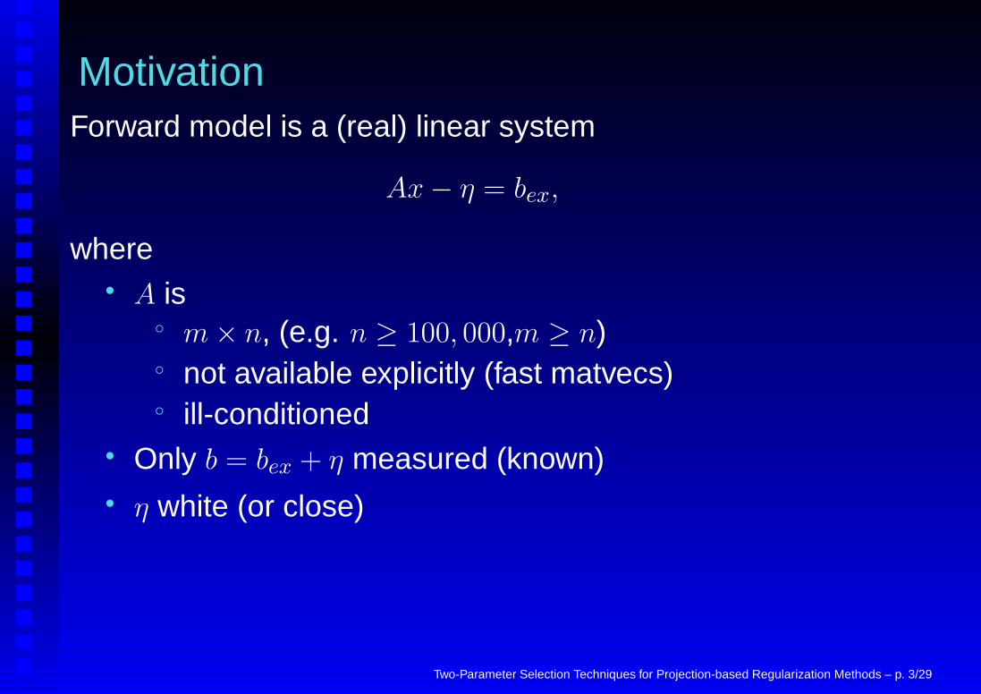
MotivationForward model is a (real) linear system
Ax− η = bex,
where• A is
◦ m× n, (e.g. n ≥ 100, 000,m ≥ n)◦ not available explicitly (fast matvecs)◦ ill-conditioned
• Only b = bex + η measured (known)• η white (or close)
Two-Parameter Selection Techniques for Projection-based Regularization Methods – p. 3/29
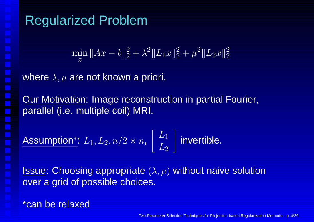
Regularized Problem
minx‖Ax− b‖22 + λ2‖L1x‖
22 + µ2‖L2x‖
22
where λ, µ are not known a priori.
Our Motivation: Image reconstruction in partial Fourier,parallel (i.e. multiple coil) MRI.
Assumption∗: L1, L2, n/2× n,[
L1
L2
]
invertible.
Issue: Choosing appropriate (λ, µ) without naive solutionover a grid of possible choices.
*can be relaxedTwo-Parameter Selection Techniques for Projection-based Regularization Methods – p. 4/29
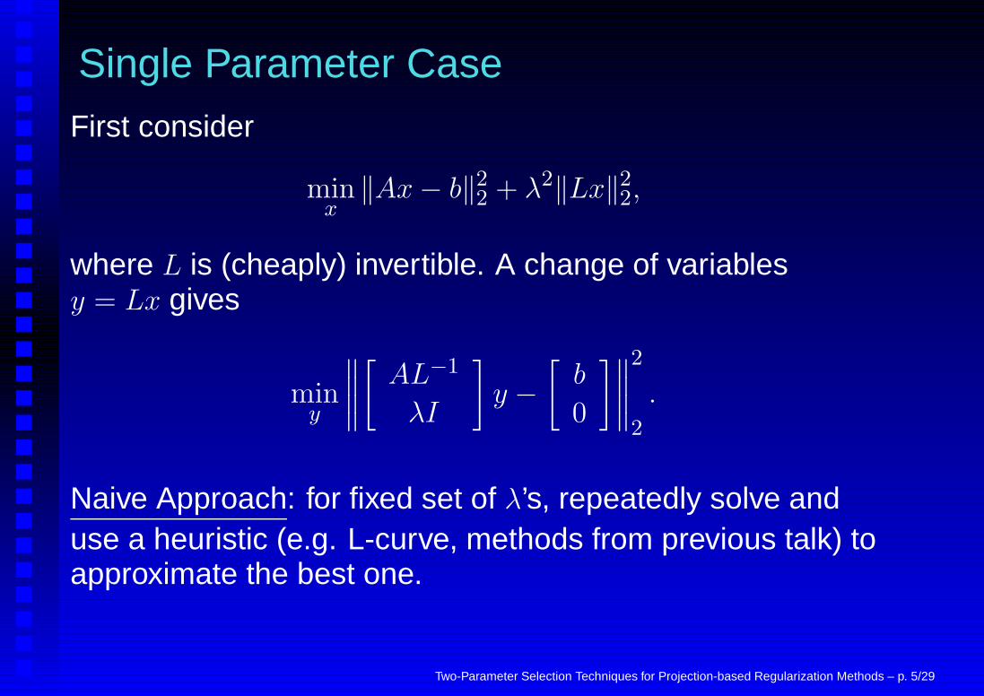
Single Parameter CaseFirst consider
minx‖Ax− b‖22 + λ2‖Lx‖22,
where L is (cheaply) invertible. A change of variablesy = Lx gives
miny
∥
∥
∥
∥
[
AL−1
λI
]
y −
[
b
0
]∥
∥
∥
∥
2
2
.
Naive Approach: for fixed set of λ’s, repeatedly solve anduse a heuristic (e.g. L-curve, methods from previous talk) toapproximate the best one.
Two-Parameter Selection Techniques for Projection-based Regularization Methods – p. 5/29
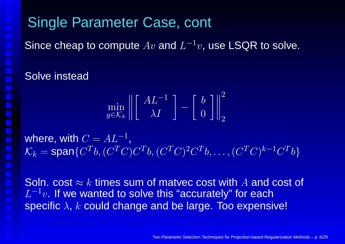
Single Parameter Case, cont
Since cheap to compute Av and L−1v, use LSQR to solve.
Solve instead
miny∈Kk
∥
∥
∥
∥
[
AL−1
λI
]
−
[
b
0
]∥
∥
∥
∥
2
2
where, with C = AL−1,Kk = span{CT b, (CT C)CT b, (CTC)2CT b, . . . , (CT C)k−1CT b}
Soln. cost ≈ k times sum of matvec cost with A and cost ofL−1v. If we wanted to solve this “accurately” for eachspecific λ, k could change and be large. Too expensive!
Two-Parameter Selection Techniques for Projection-based Regularization Methods – p. 6/29
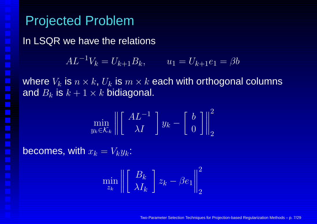
Projected ProblemIn LSQR we have the relations
AL−1Vk = Uk+1Bk, u1 = Uk+1e1 = βb
where Vk is n× k, Uk is m× k each with orthogonal columnsand Bk is k + 1× k bidiagonal.
minyk∈Kk
∥
∥
∥
∥
[
AL−1
λI
]
yk −
[
b
0
]∥
∥
∥
∥
2
2
becomes, with xk = Vkyk:
minzk
∥
∥
∥
∥
[
Bk
λIk
]
zk − βe1
∥
∥
∥
∥
2
2
Two-Parameter Selection Techniques for Projection-based Regularization Methods – p. 7/29
Regularized, Projected Problem
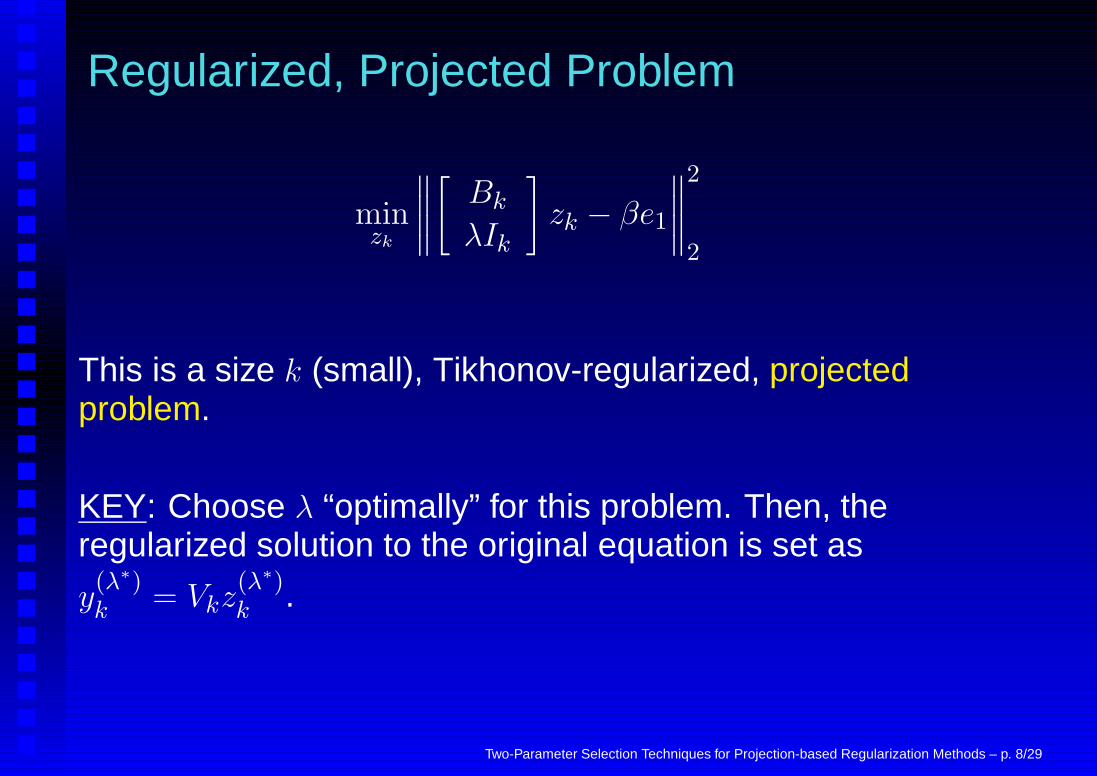
minzk
∥
∥
∥
∥
[
Bk
λIk
]
zk − βe1
∥
∥
∥
∥
2
2
This is a size k (small), Tikhonov-regularized, projectedproblem.
KEY: Choose λ “optimally” for this problem. Then, theregularized solution to the original equation is set as
y(λ∗)k = Vkz
(λ∗)k .
Two-Parameter Selection Techniques for Projection-based Regularization Methods – p. 8/29
Benefits
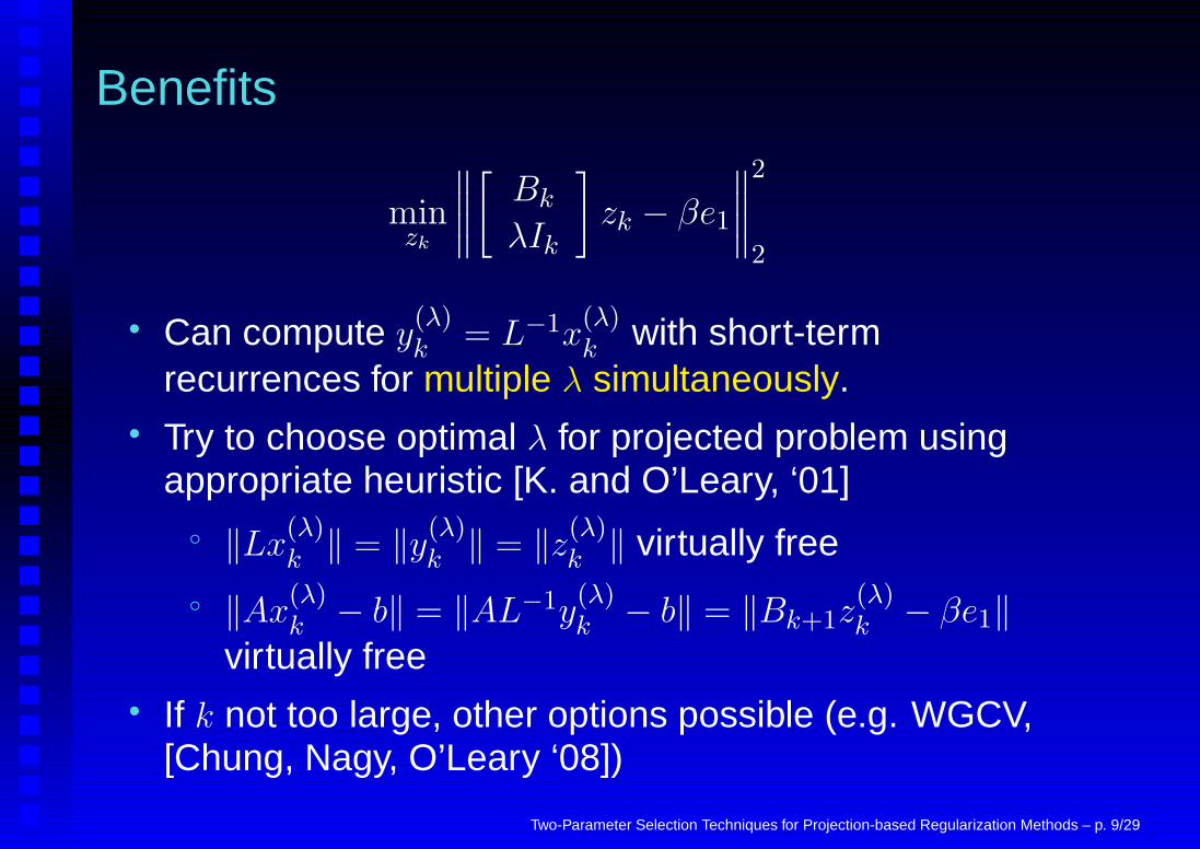
minzk
∥
∥
∥
∥
[
Bk
λIk
]
zk − βe1
∥
∥
∥
∥
2
2
• Can compute y(λ)k = L−1x
(λ)k with short-term
recurrences for multiple λ simultaneously.• Try to choose optimal λ for projected problem using
appropriate heuristic [K. and O’Leary, ‘01]◦ ‖Lx
(λ)k ‖ = ‖y
(λ)k ‖ = ‖z
(λ)k ‖ virtually free
◦ ‖Ax(λ)k − b‖ = ‖AL−1y
(λ)k − b‖ = ‖Bk+1z
(λ)k − βe1‖
virtually free• If k not too large, other options possible (e.g. WGCV,
[Chung, Nagy, O’Leary ‘08])
Two-Parameter Selection Techniques for Projection-based Regularization Methods – p. 9/29
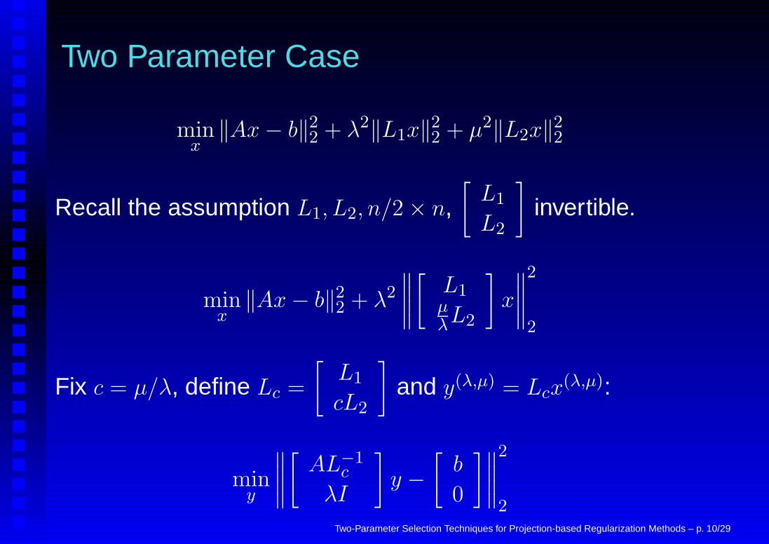
Two Parameter Case
minx‖Ax− b‖22 + λ2‖L1x‖
22 + µ2‖L2x‖
22
Recall the assumption L1, L2, n/2× n,[
L1
L2
]
invertible.
minx‖Ax− b‖22 + λ2
∥
∥
∥
∥
[
L1µλL2
]
x
∥
∥
∥
∥
2
2
Fix c = µ/λ, define Lc =
[
L1
cL2
]
and y(λ,µ) = Lcx(λ,µ):
miny
∥
∥
∥
∥
[
AL−1c
λI
]
y −
[
b
0
]∥
∥
∥
∥
2
2Two-Parameter Selection Techniques for Projection-based Regularization Methods – p. 10/29
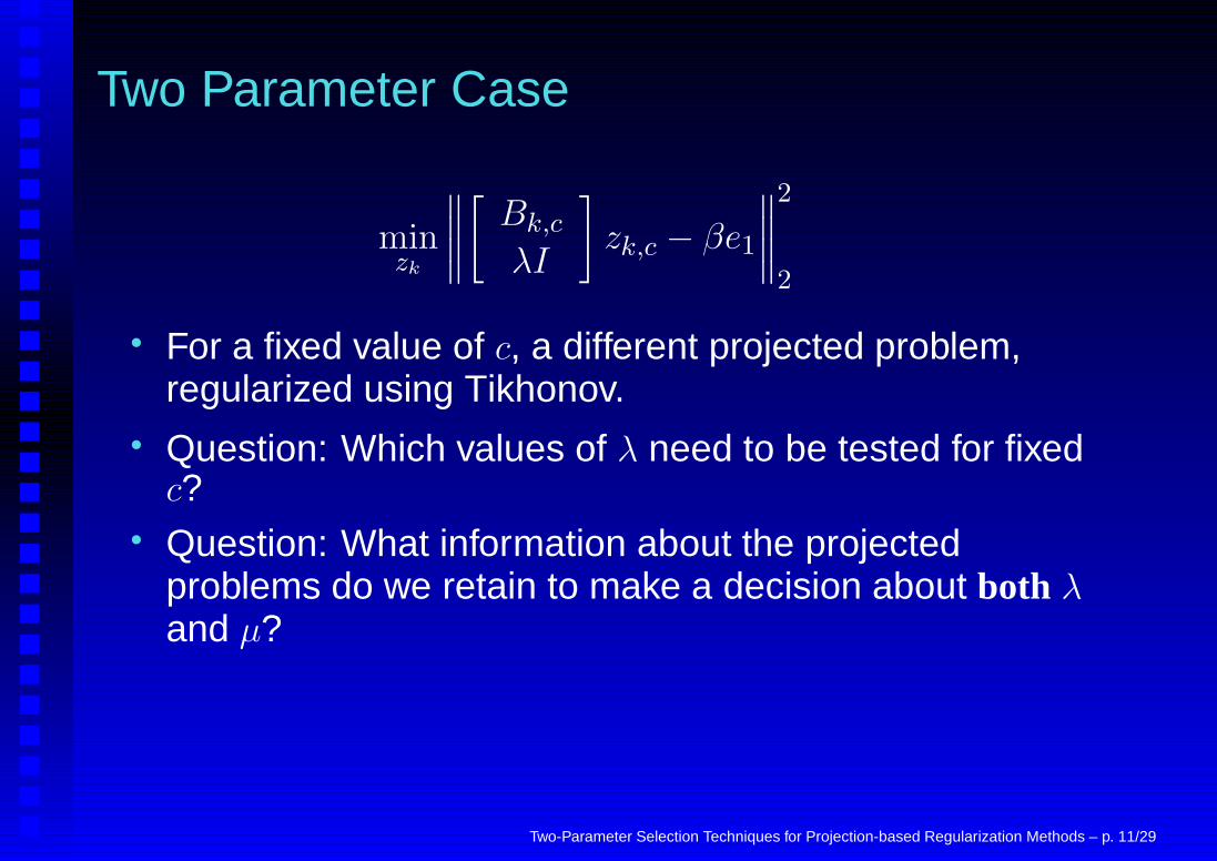
Two Parameter Case
minzk
∥
∥
∥
∥
[
Bk,c
λI
]
zk,c − βe1
∥
∥
∥
∥
2
2
• For a fixed value of c, a different projected problem,regularized using Tikhonov.
• Question: Which values of λ need to be tested for fixedc?
• Question: What information about the projectedproblems do we retain to make a decision about both λand µ?
Two-Parameter Selection Techniques for Projection-based Regularization Methods – p. 11/29
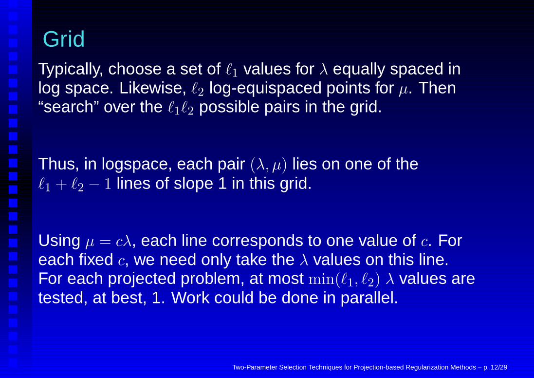
GridTypically, choose a set of `1 values for λ equally spaced inlog space. Likewise, `2 log-equispaced points for µ. Then“search” over the `1`2 possible pairs in the grid.
Thus, in logspace, each pair (λ, µ) lies on one of the`1 + `2 − 1 lines of slope 1 in this grid.
Using µ = cλ, each line corresponds to one value of c. Foreach fixed c, we need only take the λ values on this line.For each projected problem, at most min(`1, `2) λ values aretested, at best, 1. Work could be done in parallel.
Two-Parameter Selection Techniques for Projection-based Regularization Methods – p. 12/29
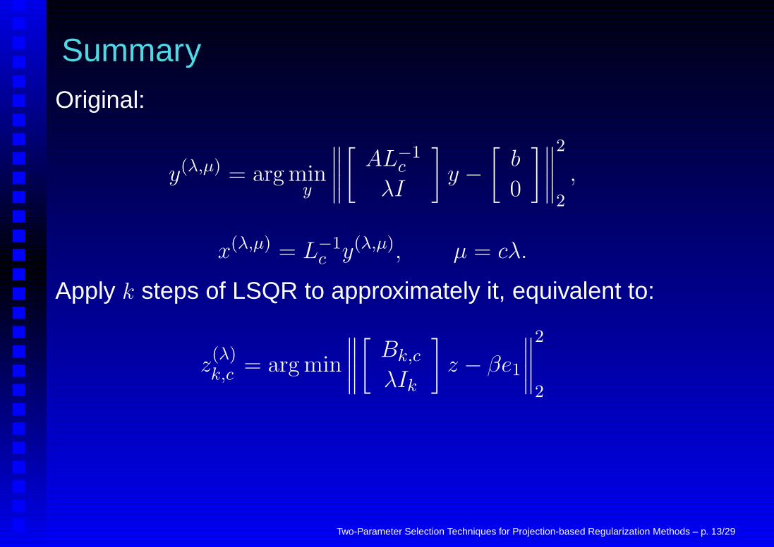
SummaryOriginal:
y(λ,µ) = arg miny
∥
∥
∥
∥
[
AL−1c
λI
]
y −
[
b
0
]∥
∥
∥
∥
2
2
,
x(λ,µ) = L−1c y(λ,µ), µ = cλ.
Apply k steps of LSQR to approximately it, equivalent to:
z(λ)k,c = arg min
∥
∥
∥
∥
[
Bk,c
λIk
]
z − βe1
∥
∥
∥
∥
2
2
Two-Parameter Selection Techniques for Projection-based Regularization Methods – p. 13/29
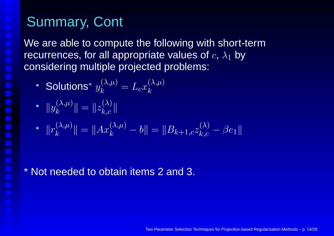
Summary, ContWe are able to compute the following with short-termrecurrences, for all appropriate values of c, λ1 byconsidering multiple projected problems:
• Solutions∗ y(λ,µ)k = Lcx
(λ,µ)k
• ‖y(λ,µ)k ‖ = ‖z
(λ)k,c ‖
• ‖r(λ,µ)k ‖ = ‖Ax
(λ,µ)k − b‖ = ‖Bk+1,cz
(λ)k,c − βe1‖
* Not needed to obtain items 2 and 3.
Two-Parameter Selection Techniques for Projection-based Regularization Methods – p. 14/29
GoalCompute near “optimal” values of λ, µ. Would like to do thisusing only information that was cheaply computed for eachprojected problem.
Following single-parameter case logic, knowing an “optimal”value of λ for each fixed-c line might be useful.
Added difficulty: each projected problem depends on afixed choice of c, but need whole picture. In particular,
‖Lcx(λ,µ)k ‖ is what is returned, not ‖L1x
(λ,µ)k ‖, ‖L2x
(λ,µ)k ‖.
Two-Parameter Selection Techniques for Projection-based Regularization Methods – p. 15/29
Regularization Parameter Selection
Scheme somewhat problem specific, main idea but may beuseful in other applications as well.
For each c, select regularization parameter λ for thecorresponding projected problem. Using µ = cλ, gives us`1 + `2 − 1 possible choices. Next use other (problemdependent) a priori information to select from among these.
For our application, enough to monitor sharp transitions inresidual norms (cheap, available).
Two-Parameter Selection Techniques for Projection-based Regularization Methods – p. 16/29
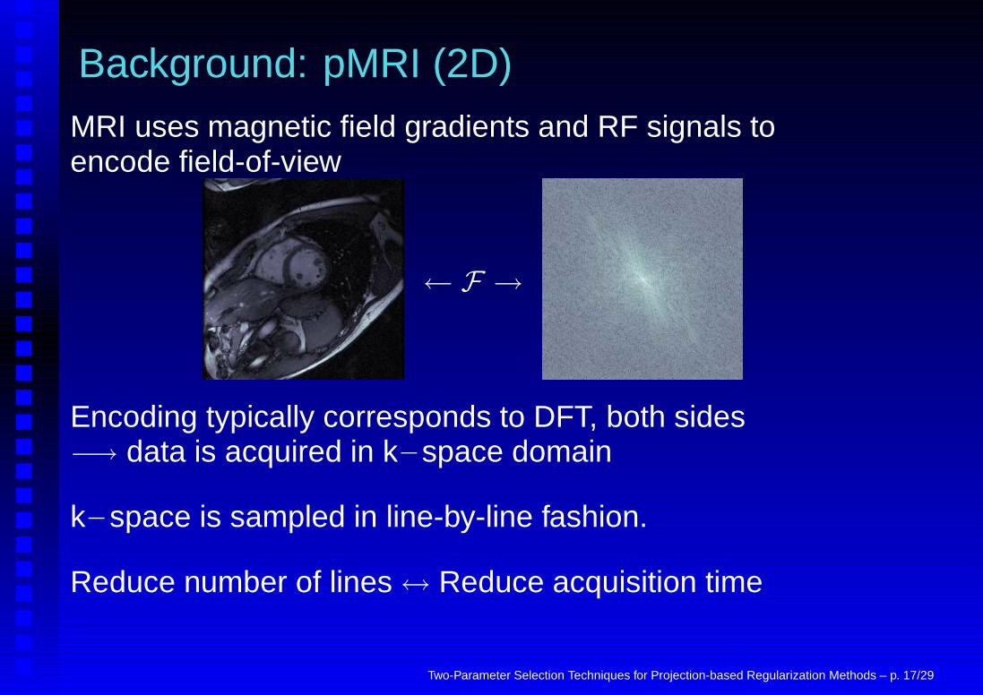
Background: pMRI (2D)MRI uses magnetic field gradients and RF signals toencode field-of-view
← F →
Encoding typically corresponds to DFT, both sides−→ data is acquired in k space domain
k space is sampled in line-by-line fashion.
Reduce number of lines↔ Reduce acquisition time
Two-Parameter Selection Techniques for Projection-based Regularization Methods – p. 17/29

2D pMRISub-sampling k-space produces aliasing in spatial domain.
← F →
Use multiple receiver coilsand each coil subsamples in parallel. 4coils, each subsampling by 4→ 16 min.scan now takes 4 min.
����
����
W2
W34
W1
W
Reconstruct image one column at a time (regularized soln.to Wρ = s).Similarly, 3D, reconstruct volume one 2D image slice at atime. Two-Parameter Selection Techniques for Projection-based Regularization Methods – p. 18/29
Fast imaging using partial-Fourier encoding
Strategy: • Acquire one half of k-space (top 1/2)• Use conjugate-symmetry assumption to
reconstruct the other half
Issues: • Conjugate-symmetry implies a real-valuedimage
• Field inhomogeneity and gradient fielderrors prevent exact conjugate-symmetryin k-space encoding.
Two-Parameter Selection Techniques for Projection-based Regularization Methods – p. 19/29
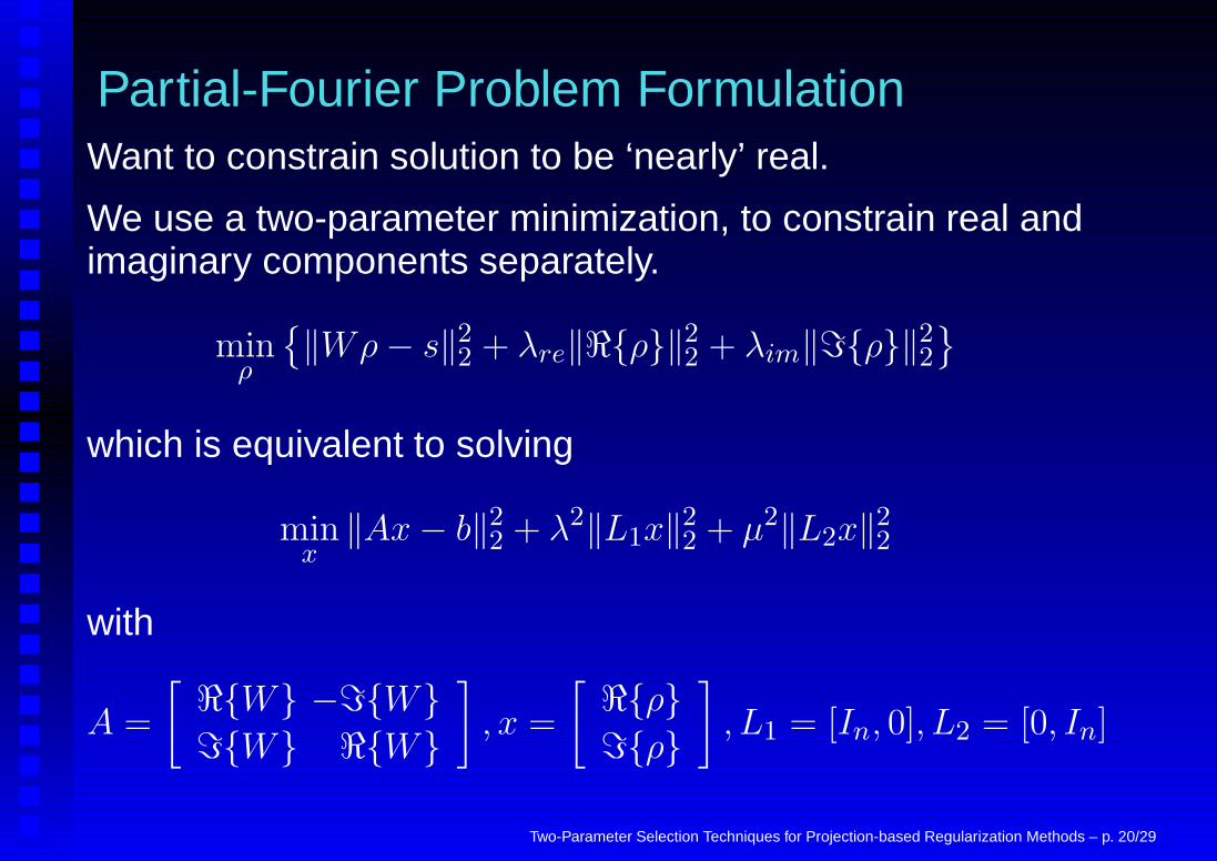
Partial-Fourier Problem FormulationWant to constrain solution to be ‘nearly’ real.
We use a two-parameter minimization, to constrain real andimaginary components separately.
minρ
{
‖Wρ− s‖22 + λre‖<{ρ}‖22 + λim‖={ρ}‖
22
}
which is equivalent to solving
minx‖Ax− b‖22 + λ2‖L1x‖
22 + µ2‖L2x‖
22
with
A =
[
<{W} −={W}
={W} <{W}
]
, x =
[
<{ρ}
={ρ}
]
, L1 = [In, 0], L2 = [0, In]
Two-Parameter Selection Techniques for Projection-based Regularization Methods – p. 20/29

Parameter SelectionSTEP 1: For each c (line) do:
• Compute the residual norms, as function of λ1, for theprojected problem (cheap!). Note these are the sameas residual norms corresponding to the large problem.
• Compute relative difference between neighboringterms on that line.
• Record λ value corresponding the sharpest transition.
STEP 2:
• If haven’t already, compute the xλ,µk ’s for these pairs.
• Throw out any “non-physical” solutions (e.g. ratio ofimaginary part to real part too large).
• Choose the remaining term with smallest residualnorm.
Two-Parameter Selection Techniques for Projection-based Regularization Methods – p. 21/29
Numerical ResultsHigh resolution phantom, 8 coil GE Scanner at BWH, single256x256 slice of 3D data set
• Sampled (partial Fourier) in ky-space 73 lines (at orabove 128); Sampled in kx-space 114 lines,nonuniformly.
• Acceleration factor ≈ 8• A is 133,152 x 131,072• λ1 = logspace(-5,2,10); λ2 = logspace(-3,4,10)• k fixed at 30• Simple thresholding on aliased image to throw out
non-physical solutions.
Two-Parameter Selection Techniques for Projection-based Regularization Methods – p. 22/29
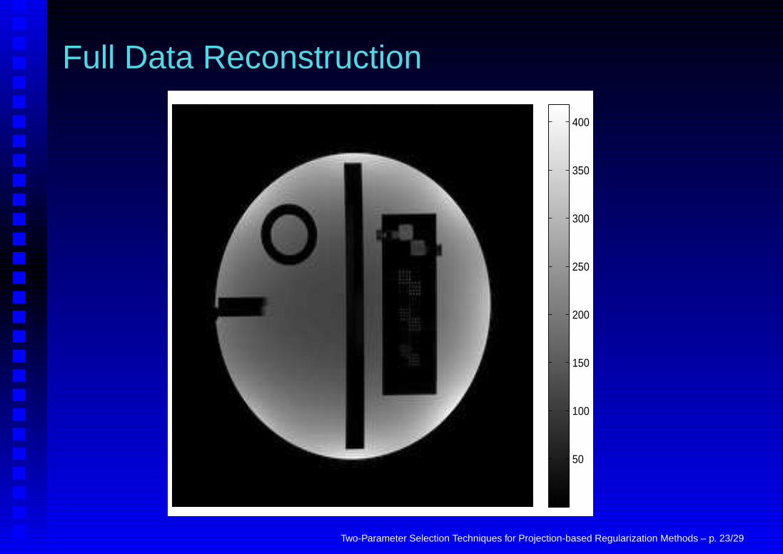
Full Data Reconstruction
50
100
150
200
250
300
350
400
Two-Parameter Selection Techniques for Projection-based Regularization Methods – p. 23/29
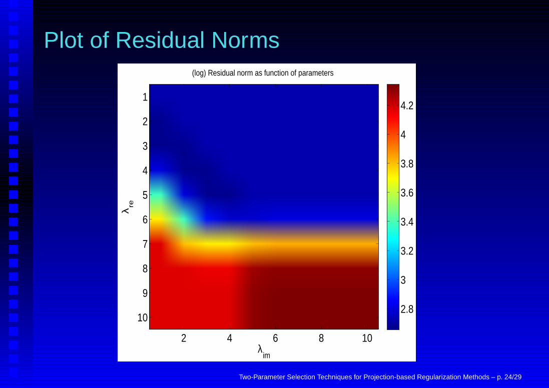
Plot of Residual Norms
λim
λre
(log) Residual norm as function of parameters
2 4 6 8 10
1
2
3
4
5
6
7
8
9
102.8
3
3.2
3.4
3.6
3.8
4
4.2
Two-Parameter Selection Techniques for Projection-based Regularization Methods – p. 24/29
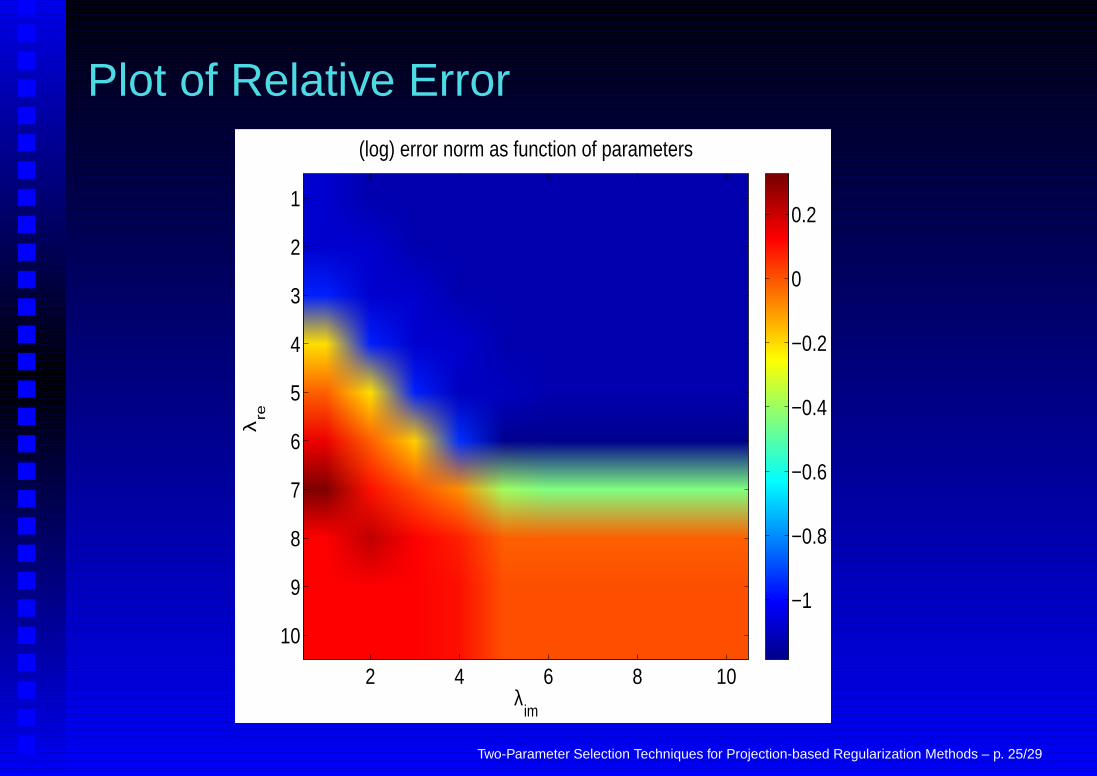
Plot of Relative Error
λim
λre
(log) error norm as function of parameters
2 4 6 8 10
1
2
3
4
5
6
7
8
9
10
−1
−0.8
−0.6
−0.4
−0.2
0
0.2
Two-Parameter Selection Techniques for Projection-based Regularization Methods – p. 25/29
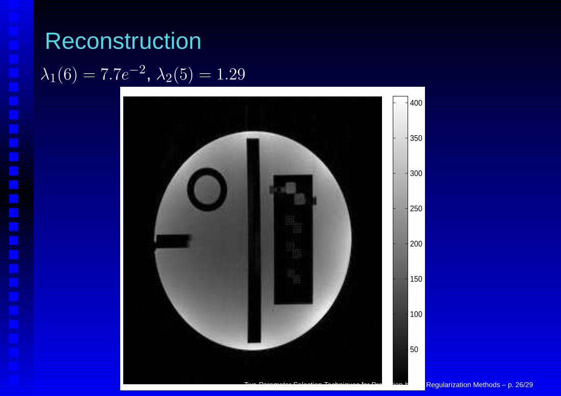
Reconstructionλ1(6) = 7.7e−2, λ2(5) = 1.29
50
100
150
200
250
300
350
400
Two-Parameter Selection Techniques for Projection-based Regularization Methods – p. 26/29
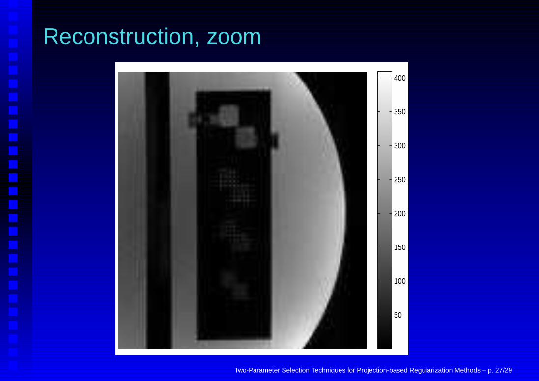
Reconstruction, zoom
50
100
150
200
250
300
350
400
Two-Parameter Selection Techniques for Projection-based Regularization Methods – p. 27/29
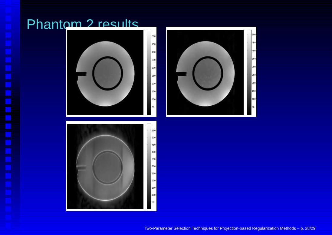
Phantom 2 results
50
100
150
200
250
300
350
400
450
500
50
100
150
200
250
300
350
400
450
500
50
100
150
200
250
300
350
400
450
500
550
Two-Parameter Selection Techniques for Projection-based Regularization Methods – p. 28/29
Conclusions and Future Work• Projection approaches can be very computationally
efficient – choose the regularization parameter for thesmaller, projected problem (cheaper).
• For 2D, we select first for individual projectedproblems, then over the whole.
• Best selection methods may be problem dependent.• Basic idea valid when L1, L2 not this special: Transform
to standard form or use hybrid approach of [K.,Hansen, Espanol, ‘07].
• Issue of choosing k [Chung, Nagy, O’Leary ‘08]. Not afactor for our application.
Two-Parameter Selection Techniques for Projection-based Regularization Methods – p. 29/29