Embed Size (px)
Citation preview

Regularization of Least Squares Problems
Heinrich [email protected]
Hamburg University of TechnologyInstitute of Numerical Simulation
TUHH Heinrich Voss Least Squares Problems Valencia 2010 1 / 82

Outline
1 Introduction
2 Least Squares Problems
3 Ill-conditioned problems
4 Regularization
5 Large problems
TUHH Heinrich Voss Least Squares Problems Valencia 2010 2 / 82

Introduction
Well-posed / ill-posed problems
Back in 1923 Hadamard introduced the concept of well-posed and ill-posedproblems.
A problem is well-posed, if— it is solvable— its solution is unique— its solution depends continuously on system parameters
(i.e. arbitrary small perturbation of the data can not cause arbitrary largeperturbation of the solution)
Otherwise it is ill-posed.
According to Hadamard’s philosophy, ill-posed problems are actually ill-posed,in the sense that the underlying model is wrong.
TUHH Heinrich Voss Least Squares Problems Valencia 2010 4 / 82

Introduction
Ill-posed problems
Ill-posed problems often arise in the form of inverse problems in many areasof science and engineering.
Ill-posed problems arise quite naturally if one is interested in determining theinternal structure of a physical system from the system’s measured behavior,or in determining the unknown input that gives rise to a measured outputsignal.
Examples are— computerized tomography, where the density inside a body is
reconstructed from the loss of intensity at detectors when scanning thebody with relatively thin X-ray beams, and thus tumors or other anomaliesare detected.
— solving diffusion equations in negative time direction to detect the sourceof pollution from measurements
Further examples appear in acoustics, astrometry, electromagnetic scattering,geophysics, optics, image restoration, signal processing, and others.
TUHH Heinrich Voss Least Squares Problems Valencia 2010 5 / 82

Least Squares Problems
Least Squares ProblemsLet
‖Ax − b‖ = min! where A ∈ Rm×n, b ∈ Rm,m ≥ n. (1)
Differentiatingϕ(x) = ‖Ax − b‖2
2 = (Ax − b)T (Ax − b) (2)
yields the necessary condition
AT Ax = AT b. (3)
called normal equations.
If the columns of A are linearly independent, then AT A is positive definite, i.e.ϕ is strictly convex and the solution is unique.
Geometrically, x∗ is a solution of (1) if and only if the residual r := b − Ax atx∗ is orthogonal to the range of A,
b − Ax∗ ⊥ R(A). (4)
TUHH Heinrich Voss Least Squares Problems Valencia 2010 7 / 82

Least Squares Problems
Solving LS problemsIf the columns of A are linearly independent, the solution x∗ can be obtainedsolving the normal equation by the Cholesky factorization of AT A > 0.
However, AT A may be badly conditioned, and then the solution obtained thisway can be useless.
In finite arithmetic the QR-decomposition of A is a more stable approach.
If A = QR, where Q ∈ Rm×m is orthogonal, R =
[R0
], R ∈ Rn×n upper
triangular, then
‖Ax − b‖2 = ‖Q(Rx −QT b)‖2 =
∥∥∥∥[Rx − β1−β2
]∥∥∥∥2, QT b =
[β1β2
],
and the unique solution of (1) is
x∗ = R−1β1.
TUHH Heinrich Voss Least Squares Problems Valencia 2010 8 / 82

Least Squares Problems
Singular value decompositionA powerful tool for the analysis of the least squares problem is the singularvalue decomposition (SVD) of A:
A = UΣV T (5)
with orthogonal matrices U ∈ Rm×m, V ∈ Rn×n and a diagonal matrixΣ ∈ Rm×n.
A more compact form of the SVD is
A = UΣV T (6)
with the matrix U ∈ Rm×n having orthonormal columns, an orthogonal matrixV ∈ Rn×n and a diagonal matrix Σ ∈ Rn×n = diag(σ1, . . . , σn).
It is common understanding that the columns of U and V are ordered andscaled such that σj ≥ 0 are nonnegative and are ordered by magnitude:
σ1 ≥ σ2 ≥ · · · ≥ σn ≥ 0.
σi , i = 1, . . . ,n are the singular values of A, the columns of U are the leftsingular vectors and the columns of V are the right singular vectors of A.
TUHH Heinrich Voss Least Squares Problems Valencia 2010 9 / 82

Least Squares Problems
Solving LS problems cnt.With y := V T x and c := UT b it holds
‖Ax − b‖2 = ‖UΣV T x − b‖2 = ‖Σy − c‖2.
For rank(A) = r it follows
yj =cj
σj, j = 1, . . . , r and yj ∈ R arbitrary for j > r .
Hence,
x =r∑
j=1
uTj bσj
vj +n∑
j=r+1
γjvj , γj ∈ R.
Since vr+1, . . . , vn span the kernel N (A) of A, the solution set of (1) is
L = xLS +N (A) (7)
where
xLS :=r∑
j=1
uTj bσj
vj
is the solution with minimal norm called minimum norm or pseudo normalsolution of (1).
TUHH Heinrich Voss Least Squares Problems Valencia 2010 10 / 82

Least Squares Problems
Pseudoinverse
For fixed A ∈ Rm×n the mapping that maps a vector b ∈ Rm to the minimumnorm solution xLS of ‖Ax − b‖ = min! obviously is linear, and therefore isrepresented by a matrix A† ∈ Rn×m.
A† is called pseudo inverse or generalized inverse or Moore-Penrose inverseof A.
If A has full rank n, then A† = (AT A)−1AT (follows from the normal equations),and if A is quadratic and nonsingular then A† = A−1.
For general A = UΣV T it follows from the representation of xLS that
A† = V Σ†UT , Σ† = diagτi, τi =
1/σi if σi > 0
0 if σi = 0
TUHH Heinrich Voss Least Squares Problems Valencia 2010 11 / 82

Least Squares Problems
Perturbation Theorem
Let the matrix A ∈ Rm×n, m ≥ n have full rank, let x be the unique solution ofthe least squares problem (1), and let x be the solution of a perturbed leastsquares problem
‖(A + δA)x − (b + δb)‖ = min! (8)
where the perturbation is not too large in the sense
ε := max(‖δA‖‖A‖
,‖δb‖‖b‖
)<
1κ2(A)
(9)
where κ2(A) := σ1/σn denotes the condition number of A.
Then it holds that
‖x − x‖‖x‖
≤ ε(
2κ2(A)
cos(θ)+ tan(θ) · κ2
2(A)
)+O(ε2) (10)
where θ is the angle between b and its projection onto R(A).
For a proof see the book of J. Demmel, Applied Linear Algebra.
TUHH Heinrich Voss Least Squares Problems Valencia 2010 12 / 82

Ill-conditioned problems
Ill-conditioned problems
In this talk we consider ill-conditioned problems (with large conditionnumbers), where small perturbations in the data A and b lead to largechanges of the least squares solution xLS.
When the system is not consistent, i.e. it holds that r = b − AxLS 6= 0, then inequation (10) it holds that tan(θ) 6= 0 which means that the relative error of theleast squares solution is roughly proportional to the square of the conditionnumber κ2(A).
When doing calculations in finite precision arithmetic the meaning of ’large’ iswith respect to the reciprocal of the machine precision.A large κ2(A) then leads to an unstable behavior of the computed leastsquares solution, i.e. in this case the solution x typically is physicallymeaningless.
TUHH Heinrich Voss Least Squares Problems Valencia 2010 14 / 82

Ill-conditioned problems
A toy problem
Consider the problem to determine the orthogonal projection of a givenfunction f : [0,1]→ R to the space Πn−1 of polynomials of degree n − 1 withrespect to the scalar product
〈f ,g〉 :=
∫ 1
0f (x)g(x) dx .
Choosing the (unfeasible) monomial basis 1, x , . . . , xn−1 this leads to thelinear system
Ay = b (1)
whereA = (aij )i,j=1,...,n, aij :=
1i + j − 1
, (2)
is the so called Hilbert matrix, and b ∈ Rn, bi := 〈f , x i−1〉.
TUHH Heinrich Voss Least Squares Problems Valencia 2010 15 / 82

Ill-conditioned problems
A toy problem cnt.
For dimensions n = 10, n = 20 and n = 40 we choose the right hand side bsuch that y = (1, . . . ,1)T is the unique solution.
Solving the problem with LU-factorization (in MATLAB A\b), the Choleskydecomposition, the QR factorization of A and the singular valuedecomposition of A we obtain the following errors in Euclidean norm:
n = 10 n = 20 n = 40LU factorization 5.24 E-4 8.25 E+1 3.78 E+2Cholesky 7.07 E-4 numer. not pos. def.QR decomposition 1.79 E-3 1.84 E+2 7.48 E+3SVD 1.23 E-5 9.60 E+1 1.05 E+3κ(A) 1.6 E+13 1.8 E+18 9.8 E+18 (?)
TUHH Heinrich Voss Least Squares Problems Valencia 2010 16 / 82
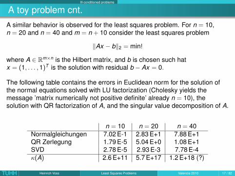
Ill-conditioned problems
A toy problem cnt.A similar behavior is observed for the least squares problem. For n = 10,n = 20 and n = 40 and m = n + 10 consider the least squares problem
‖Ax − b‖2 = min!
where A ∈ Rm×n is the Hilbert matrix, and b is chosen such hatx = (1, . . . ,1)T is the solution with residual b − Ax = 0.
The following table contains the errors in Euclidean norm for the solution ofthe normal equations solved with LU factorization (Cholesky yields themessage ’matrix numerically not positive definite’ already n = 10), thesolution with QR factorization of A, and the singular value decomposition of A.
n = 10 n = 20 n = 40Normalgleichungen 7.02 E-1 2.83 E+1 7.88 E+1QR Zerlegung 1.79 E-5 5.04 E+0 1.08 E+1SVD 2.78 E-5 2.93 E-3 7.78 E-4κ(A) 2.6 E+11 5.7 E+17 1.2 E+18 (?)
TUHH Heinrich Voss Least Squares Problems Valencia 2010 17 / 82

Ill-conditioned problems
Rank deficient problems
In rank-deficient problems there exist a well-determined gap between largeand small singular values of A.
Often the exact rank of the matrix A ∈ Rm×n is equal to n, with a cluster ofvery small singular values that are almost zero. This cluster can simply resultfrom an overdetermined linear system that is nearly consistent. The numberof singular values that do not correspond to the cluster at zero is denoted asthe numerical rank of A.
Methods for solving rank-deficient problems try to determine the numericalrank of A, which itself is a well-conditioned problem. If the numerical rank isknown, it is usually possible to eliminate the ill-conditioning. The problem isthen reduced to a well-conditioned LS problem of smaller size.
In this talk we concentrate on discrete ill-posed problems
TUHH Heinrich Voss Least Squares Problems Valencia 2010 18 / 82

Ill-conditioned problems
Rank deficient problems cnt.
0 5 10 15 20 25 3010
−40
10−30
10−20
10−10
100
singular values of rank deficient matrix
TUHH Heinrich Voss Least Squares Problems Valencia 2010 19 / 82

Ill-conditioned problems
Fredholm integral equation of the first kindFamous representatives of ill-posed problems are Fredholm integral equationsof the first kind that are almost always ill-posed.
∫Ω
K (s, t)f (t)dt = g(s), s ∈ Ω (11)
with a given kernel function K ∈ L2(Ω2) and right-hand side functiong ∈ L2(Ω).
Then with the singular value expansion
K (s, t) =∞∑j=1
µjuj (s)vj (s), µ1 ≥ µ2 ≥ · · · ≥ 0
a solution of (11) can be expressed as
f (t) =∞∑j=1
〈uj ,g〉µj
vj (t), 〈uj ,g〉 =
∫Ω
uj (s)g(s) ds.
TUHH Heinrich Voss Least Squares Problems Valencia 2010 20 / 82

Ill-conditioned problems
Fredholm integral equation of the first kind cnt.
The solution f is square integrable if the right hand side g satisfies the Picardcondition
∞∑j=1
(〈uj ,g〉µj
)2
<∞.
The Picard condition says that from some index j on the absolute value of thecoefficients 〈uj ,g〉 must decay faster than the corresponding singular valuesµj in order that a square integrable solution exists.
For g to be square integrable the coefficients 〈uj ,g〉 must decay faster than1/√
j , but the Picard condition puts a stronger requirement on g: thecoefficients must decay faster than µj/
√j .
TUHH Heinrich Voss Least Squares Problems Valencia 2010 21 / 82

Ill-conditioned problems
Discrete ill-posed problems
Discretizing a Fredholm integral equation results in discrete ill-posed problems
Ax = b
.
The matrix A inherits the following properties from the continuous problem(11): it is ill-conditioned with singular values gradually decaying to zero.
This is the main difference to rank-deficient problems.Discrete ill-posed problems have an ill-determined rank, i.e. theredoes not exist a gap in the singular values that could be used as anatural threshold.
TUHH Heinrich Voss Least Squares Problems Valencia 2010 22 / 82

Ill-conditioned problems
Discrete ill-posed problems cnt.
0 5 10 15 20 25 3010
−35
10−30
10−25
10−20
10−15
10−10
10−5
100
Singular values of discrete ill posed problem
TUHH Heinrich Voss Least Squares Problems Valencia 2010 23 / 82
Ill-conditioned problems
Discrete ill-posed problems cnt.
When the continuous problem satisfies the Picard condition, then the absolutevalues of the Fourier coefficients uT
i b decay gradually to zero with increasingi , where ui is the i th left singular vector obtained from the SVD of A.
Typically the number of sign changes of the components of the singularvectors ui and vi increases with the index i , this means that low-frequencycomponents correspond to large singular values and the smaller singularvalues correspond to singular vectors with many oscillations.
The Picard condition translates to the following discrete Picard condition:
With increasing index i, the coefficients |uTi b| on average decay
faster to zero than σi .
TUHH Heinrich Voss Least Squares Problems Valencia 2010 24 / 82

Ill-conditioned problems
Discrete ill-posed problems cnt.The typical situation in least squares problems is the following:Instead of the exact right-hand side b a vector b = b + εs with small ε > 0 andrandom noise vector s is given. The perturbation results from measurement ordiscretization errors.
The goal is to recover the solution xtrue of the underlying consistent system
Axtrue = b (12)
from the system Ax ≈ b, i.e. by solving the least squares problem
‖∆b‖ = min! subject to Ax = b + ∆b. (13)
For the solution it holds
xLS = A†b =r∑
i=1
uTi bσi
vi + ε
r∑i=1
uTi sσi
vi (14)
where r is the rank of A.TUHH Heinrich Voss Least Squares Problems Valencia 2010 25 / 82

Ill-conditioned problems
Discrete ill-posed problems cnt.
The solution consists of two terms, the first one is the true solution xtrue andthe second term is the contribution from the noise.
If the vector s consists of uncorrelated noise, the parts of s into the directionsof the left singular vectors stay roughly constant, i.e. uT
i s will not vary muchfor all i . Hence the second term uT
i s/σi blows up with increasing i .
The first term contains the parts of the exact right-hand side b developed intothe directions of the left singular vectors, i.e. the Fourier coefficients uT
i b.
If the discrete Picard condition is satisfied, then xLS is dominated by theinfluence of the noise, i.e. the solution will mainly consist of a linearcombination of right singular vectors corresponding to the smallest singularvalues of A.
TUHH Heinrich Voss Least Squares Problems Valencia 2010 26 / 82

Regularization
Regularization
Assume A has full rank . Then a regularized solution can be written in the form
xreg = V ΘΣ†UT b =n∑
i=1
fiuT
i bσi
vi =n∑
i=1
fiuT
i bσi
vi + ε
n∑i=1
fiuT
i sσi
vi . (15)
Here the matrix Θ ∈ Rn×n is a diagonal matrix, with the so called filter factorsfi on its diagonal.
A suitable regularization method adjusts the filter factors in such a way thatthe unwanted components of the SVD are damped whereas the wantedcomponents remain essentially unchanged.
Most regularization methods are much more efficient when the discrete Picardcondition is satisfied. But also when this condition does not hold the methodsperform well in general.
TUHH Heinrich Voss Least Squares Problems Valencia 2010 28 / 82

Regularization
Truncated SVDOne of the simplest regularization methods is the truncated singular valuedecomposition (TSVD). In the TSVD method the matrix A is replaced by itsbest rank-k approximation, measured in the 2-norm or the Frobenius norm
Ak =k∑
i=1
σiuivTi with ‖A− Ak‖2 = σk+1. (16)
The approximate solution xk for problem (13) is then given by
xk = A†k b =k∑
i=1
uTi bσi
vi =k∑
i=1
uTi bσi
vi + ε
k∑i=1
uTi sσi
vi (17)
or in terms of the filter coefficients we simply have the regularized solution(15) with
fi =
1 for i ≤ k0 for i > k (18)
TUHH Heinrich Voss Least Squares Problems Valencia 2010 29 / 82

Regularization
Truncated SVD cnt.
The solution xk does not contain any high frequency components, i.e. allsingular values starting from the index k + 1 are set to zero and thecorresponding singular vectors are disregarded in the solution. So the termuT
i s/σi in equation (17) corresponding to the noise s is prevented fromblowing up.
The TSVD method is particularly suitable for rank-deficient problems. When kreaches the numerical rank r of A the ideal approximation xr is found.
For discrete ill-posed problems the TSVD method can be applied as well,although the cut off filtering strategy is not the best choice when facinggradually decaying singular values of A.
TUHH Heinrich Voss Least Squares Problems Valencia 2010 30 / 82

Regularization
ExampleSolution of the Fredholm integral equation shaw from Hansen’s regularizationtool of dimension 40
−1.5 −1 −0.5 0 0.5 1 1.50
0.5
1
1.5
2
2.5exact solution of shaw; dim=40
TUHH Heinrich Voss Least Squares Problems Valencia 2010 31 / 82

Regularization
ExampleSolution of the Fredholm integral equation shaw from Hansen’s regularizationtool of dimension 40 and its approximation via LU factorization
−1.5 −1 −0.5 0 0.5 1 1.5−30
−20
−10
0
10
20
30exact solution of shaw and LU appr.; dim=40
TUHH Heinrich Voss Least Squares Problems Valencia 2010 32 / 82

Regularization
ExampleSolution of the Fredholm integral equation shaw from Hansen’s regularizationtool of dimension 40 and its approximation via complete SVD
−1.5 −1 −0.5 0 0.5 1 1.5−150
−100
−50
0
50
100
150
200exact solution of shaw and SVD appr.; dim=40
TUHH Heinrich Voss Least Squares Problems Valencia 2010 33 / 82

Regularization
ExampleSolution of the Fredholm integral equation shaw from Hansen’s regularizationtool of dimension 40 and its approximation via truncated SVD
−1.5 −1 −0.5 0 0.5 1 1.50
0.5
1
1.5
2
2.5exact solution of shaw and truncated SVD appr.; dim=40
blue:exactgreen:k=5red:k=10
TUHH Heinrich Voss Least Squares Problems Valencia 2010 34 / 82

Regularization
Tikhonov regularization
In Tikhonov regularization (introduced independently by Tikhonov (1963) andPhillips (1962)) the approximate solution xλ is defined as minimizer of thequadratic functional
‖Ax − b‖2 + λ‖Lx‖2 = min! (19)
The basic idea of Tikhonov regularization is the following: Minimizing thefunctional in (19) means to search for some xλ, providing at the same time asmall residual ‖Axλ − b‖ and a moderate value of the penalty function ‖Lxλ‖.
If the regularization parameter λ is chosen too small, (19) is too close to theoriginal problem and instabilities have to be expected.
If λ is chosen too large, the problem we solve has only little connection withthe original problem. Finding the optimal parameter is a tough problem.
TUHH Heinrich Voss Least Squares Problems Valencia 2010 35 / 82

Regularization
ExampleSolution of the Fredholm integral equation shaw from Hansen’s regularizationtool of dimension 40 and its approximation via Tikhonov regularization
−1.5 −1 −0.5 0 0.5 1 1.50
0.5
1
1.5
2
2.5exact solution of shaw and Tikhonov regularization; dim=40
blue:exactgreen:λ=1red:λ=1e−12
TUHH Heinrich Voss Least Squares Problems Valencia 2010 36 / 82

Regularization
Tikhonov regularization cnt.
Tikhonov regularization has an important equivalent formulation as
min ‖Ax − b‖ subject to ‖Lx‖ ≤ δ (20)
where δ is a positive constant.
(20) is a linear LS problem with a quadratic constraint, and using theLagrange multiplier formulation
L(x , λ) = ‖Ax − b‖2 + λ(‖Lx‖2 − δ2), (21)
it can be shown that if δ ≤ ‖xLS‖, where xLS denotes the LS solution of‖Ax − b‖ = min!, then the solution xδ of (20) is identical to the solution xλ of(19) for an appropriately chosen λ, and there is a monotonic relation betweenthe parameters δ and λ.
TUHH Heinrich Voss Least Squares Problems Valencia 2010 37 / 82

Regularization
Tikhonov regularization cnt.Problem (19) can be also expressed as an ordinary least squares problem:∥∥∥∥[ A√
λL
]x −
[b0
]∥∥∥∥2
= min! (22)
with the normal equations
(AT A + λLT L)x = AT b. (23)
Let the matrix Aλ := [AT ,√λLT ]T have full rank, then a unique solution exists.
For L = I (which is called the standard case) the solution xλ = xreg of (23) is
xλ = V ΘΣ†UT b =n∑
i=1
fiuT
i bσi
vi =n∑
i=1
σi (uTi b)
σ2i + λ
vi (24)
where A = UΣV T is the SVD of A. Hence, the filter factors are
fi =σ2
i
σ2i + λ
for L = I. (25)
For L 6= I a similar representation holds with the generalized SVD of (A,L).TUHH Heinrich Voss Least Squares Problems Valencia 2010 38 / 82

Regularization
Tikhonov regularization cnt.
For singular values much larger than λ the filter factors are fi ≈ 1 whereas forsingular values much smaller than λ it holds that fi ≈ σ2
i /λ ≈ 0.
The same holds for L 6= I with replacing σi by the generalized singular valuesγi .
Hence, Tikhonov regularization is damping the influence of the singularvectors corresponding to small singular values (i.e. the influence of highlyoscillating singular vectors).
Tikhonov regularization exhibits much smoother filter factors than truncatedSVD which is favorable for discrete ill-posed problems.
TUHH Heinrich Voss Least Squares Problems Valencia 2010 39 / 82

Regularization
Generalized Singular Value Decomposition
The generalized singular value decomposition (GSVD for short) is ageneralization of the SVD for matrix pairs (A,L).
The GSVD was introduced by Van Loan (1976) for analysis of matrix pencilsAT A + λLT L, λ ∈ R, and he showed that (similar to the ordinary case) thegeneralized singular values are the square roots of the eigenvalues of(AT A,LT L). The use of the GSVD in the analysis of discrete ill-posedproblems goes back to Varah (1979).
For the GSVD the number of columns of both matrices have to be identical,and typically it holds that A ∈ Rm×n and L ∈ Rp×n with m ≥ n ≥ p.
It is assumed that the regularization matrix L has full rank and that the kernelsdo not intersect, i.e. N (A) ∩N (L) = 0.
Under these conditions the following decomposition exists:
TUHH Heinrich Voss Least Squares Problems Valencia 2010 40 / 82

Regularization
Generalized Singular Value Decomposition cnt.With orthogonal matrices U ∈ Rm×m and V ∈ Rp×p and a nonsingular matrixX ∈ Rn×n
A = UΣLX−1 and L = V [M,0]X−1 (26)
where
ΣL = diag(σ1, . . . , σp,1, . . . ,1) ∈ Rm×n and M = diag(µ1, . . . , µp) ∈ Rp×p
(27)and it holds that
0 ≤ σ1 ≤ · · · ≤ σp ≤ 1 and 1 ≥ µ1 ≥ · · · ≥ µp > 0 (28)
σ2i + µ2
i = 1 for i = 1, . . . ,p. (29)
The ratios γi = σi/µi , i = 1, . . . ,p are termed generalized singular values of(A,L).
For L = In the generalized singular values γi are identical to the usual singularvalues of A, but one should be aware of the different ordering, i.e. the γi aremonotonically increasing with their index.
TUHH Heinrich Voss Least Squares Problems Valencia 2010 41 / 82
Regularization
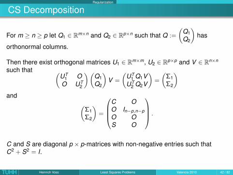
CS Decomposition
For m ≥ n ≥ p let Q1 ∈ Rm×n and Q2 ∈ Rp×n such that Q :=
(Q1Q2
)has
orthonormal columns.
Then there exist orthogonal matrices U1 ∈ Rm×m, U2 ∈ Rp×p and V ∈ Rn×n
such that (UT
1 OO UT
2
)(Q1Q2
)V =
(UT
1 Q1VUT
2 Q2V
)=
(Σ1Σ2
)and (
Σ1Σ2
)=
C OO In−p,n−pO OS O
.
C and S are diagonal p × p-matrices with non-negative entries such thatC2 + S2 = I.
TUHH Heinrich Voss Least Squares Problems Valencia 2010 42 / 82
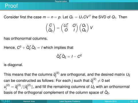
Regularization
Proof
Consider first the case m = n = p. Let Q1 = U1CV T the SVD of Q1. Then(CQ2
)=
(UT
1 OO I
)(Q1Q2
)V
has orthonormal columns.
Hence, C2 + QT2 Q2 = I which implies that
QT2 Q2 = I − C2
is diagonal.
This means that the columns q(2)j are orthogonal, and the desired matrix U2
can be constructed as follows: For each j such that q(2)j 6= 0 set
u(2)j = q(2)
j /‖q(2)j ‖, and fill the remaining columns of U2 with an orthonormal
basis of the orthogonal complement of the column space of Q2.
TUHH Heinrich Voss Least Squares Problems Valencia 2010 43 / 82

Regularization
Proof cnt.From the orthogonality of the columns of Q we have that U2 is orthogonal, and
UT2 QU2 = S where S = diags1, . . . , sp
with sj = ‖q(2)j ‖, if q(2)
j 6= 0 and sj = 0 otherwise.
This completes the proof for m = n = p.
For m ≥ n ≥ p letQ2V1 =
(Q21 O
), Q21 ∈ Rp×p
be the RQ factorization of Q2. Then(Q1Q2
)V1 =
(Q11 Q12
Q21 O
),
and the by the orthogonality
QT11Q12 = O, QT
12Q12 = I.
TUHH Heinrich Voss Least Squares Problems Valencia 2010 44 / 82

Regularization
Proof cnt.
Hence, ifU1 =
(U11 Q12
)is orthogonal, then
(UT
1 OO I
)(Q1Q2
)V1 =
UT11Q11 OO I
Q21 0
.
Since m + p − n ≥ p we may apply the QR factorization to UT11Q12 to obtain
UT1 (UT
11Q12) =
(Q11O
).
Thus, the problem is reduced to computing the CS decomposition of thesquare p × p-matrices Q11 and Q21, which completes the proof.
TUHH Heinrich Voss Least Squares Problems Valencia 2010 45 / 82
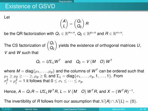
Regularization
Existence of GSVD
Let (AL
)=
(Q1Q2
)R
be the QR factorization with Q1 ∈ Rm×n, Q2 ∈ Rp×n and R ∈ Rn×n.
The CS factorization of(
Q1Q2
)yields the existence of orthogonal matrices U,
V and W such that
Q1 = UΣLW T and Q2 = V(M O
)W T
where M = diagµ1, . . . , µp and the columns of W T can be ordered such thatµ1 ≥ µ2 ≥ · · · ≥, µp ≥ 0, and ΣL = diagσ1, . . . , σp,1, . . . ,1. Fromσ2
j + µ2j = 1 it follows that 0 ≤ σ1 ≤ · · · ≤ σp.
Hence, A = Q1R = UΣLW T R, L = V(M O
)W T R, and X = (W T R)−1.
The invertibility of R follows from our assumption that N (A) ∩N (L) = 0.
TUHH Heinrich Voss Least Squares Problems Valencia 2010 46 / 82

Regularization
GSVD for discrete ill-posed problems
For general matrix pairs (A,L) little can be said about the appearance of theGSVD. However, for discrete ill-posed problems the following threecharacteristic features are often found:
— The generalized singular values σi decay towards 0 (fori = p,p − 1, . . . ,1). There is no typical gap in the spectrum separatinglarge generalized singular values from small ones.
— The singular vectors ui , vi , xi often have more sign changes in theirelements as the corresponding σi decrease. Hence, singular vectorscorresponding to tiny singular values represent highly oscillatingfunctions, whereas those corresponding to large singular valuesrepresent smooth functions. The last n − p columns of X usually havevery few sign changes.
— The Fourier coefficient of the uTi b of the right hand side on the average
decay faster to zero than the generalized singular values.
TUHH Heinrich Voss Least Squares Problems Valencia 2010 47 / 82

Regularization
Generalized Singular Value Decomposition cnt.
Let U = [Up,Um−p] and X = [Xp,Xn−p] where the index indicates the numberof columns of the corresponding matrix.
Then the columns of Xn−p span the kernel of L, i.e. N (L) = span Xn−p.
The pseudoinverse of A can be written by means of the GSVD of (A,L) as
A†L := [Xp,Xn−p]
[Σ†L 00 In−p
][Up,Un−p]T = XpΣ†LUT
p + Xn−pUTn−p. (30)
The matrix Σ†L is determined analogously to Σ†.
The solution of the least squares problem (1) is
xLS = A†b = A†Lb = XpΣ†LUTp b + Xn−pUT
n−pb =: x1L + x2
L .
Hence the solution xLS consists of two parts, the second of which x2L lies in the
nullspace of L
TUHH Heinrich Voss Least Squares Problems Valencia 2010 48 / 82
Regularization
Truncated GSVD
The idea of the truncated SVD approach can be extended to the GSVD case.
In the TGSVD method only the largest k (with k ≤ p) components of XpΣ†LUTp
are taken into account whereas the x2L remains unchanged. The solution xL,k
is given by xL,k = A†L,k b with
A†L,k := [Xp,Xn−p]
[Σ†L,k 0
0 In−p
][Up,Un−p]T = XpΣ†L,k UT
p + Xn−pUTn−p (31)
where Σ†L,k = diag(0, . . . ,0, σ−1p−k+1, . . . , σ
−1p ).
The main part of the solution xL,k now consists of k vectors from Xp, i.e.generalized singular vectors that exhibit properties of the regularization matrixL as well.
Since the GSVD is expensive to compute it should be regarded as ananalytical tool for regularizing least squares problems with a regularizationmatrix L.
TUHH Heinrich Voss Least Squares Problems Valencia 2010 49 / 82

Regularization
Tikhonov regularization via GSVD
A particularly nice feature of the GSVD is that it immediately lets us writedown a formula for the solution of the regularized solution of (19).
Introducing the filter function
fλ(γ) :=γ
γ + λ(32)
the Tikhonov approximation can be written as
xλ =
p∑j=1
fα(γ2j )
uTj bσj
xj +n∑
j=p+1
uTj bxj . (33)
Again the second (usually smooth) term xL is untouched by the regularizationwhereas the terms in the first sum are damped for γj λ (oscillatorycomponents, and due to the discrete Picard condition dominated by noise)and the other ones are only slightly changed.
TUHH Heinrich Voss Least Squares Problems Valencia 2010 50 / 82

Regularization
Implementation of Tikhonov regularizationConsider the standard form of regularization∥∥∥∥[ A√
λI
]x −
[b0
]∥∥∥∥2
= min! (34)
Multiplying A from the left and right by orthogonal matrices (which do notchange Euclidean norms) it can be transformed to bidiagonal form
A = U[
JO
]V T , U ∈ Rm×m, J ∈ Rn×n, V ∈ Rn×n
where U and V are orthogonal (which are not computed explicitly but arerepresented by a sequence of Householder transformation).
With these transformations the new right hand side is
c = UT b, c =: (cT1 , c
T2 )T , c1 ∈ Rn, c2 ∈ Rm−n
and the variable is transformed according to
x = V ξ.
TUHH Heinrich Voss Least Squares Problems Valencia 2010 51 / 82

Regularization
Implementation of Tikhonov regularization cnt.
The transformed problem reads∥∥∥∥[ J√λI
]ξ −
[c10
]∥∥∥∥2
= min! (35)
Thanks to the bidiagonal form of J, (35) can be solved very efficiently usingGivens transformations with only O(n) operations. Only these O(n)operations depend on the actual regularization parameter λ.
We considered only the standard case. If L 6= I problem (19) the problem istransformed first to standard form.
If L is square and invertible, then the standard form
‖Ax − b‖2 + λ‖x‖2 = min!
can be derived easily from x := Lx , A = AL−1 and b = b, such that the backtransformation simply is xλ = L−1xλ.
TUHH Heinrich Voss Least Squares Problems Valencia 2010 52 / 82

Regularization
Transformation into Standard Form
In the general case when L ∈ Rp×n is rectangular with full row rank p thetransformation can be performed via the GSVD.
The key step is to define the A-weighted generalized inverse of L as follows
L†A =(In − (A(In − L†L))†A
)L†. (36)
If p = n then L†L = I, and L†A = L† = L−1. For p < n however, L†A is in generaldifferent from the Moore-Penrose inverse L†.
We further need the component x0 of the regularized solution in the kernelN (L). Since I − L†L is the orthogonal projector onto N (L), it holds that
x0 = (A(In − L†L))†b.
TUHH Heinrich Voss Least Squares Problems Valencia 2010 53 / 82

Regularization
Transformation into Standard Form ct.
Given the GSVD of (A,L), L†A can be expressed as (cf. Elden 1982))
L†A = X[diagµ−1
j O
]V T . (37)
and x0 as
x0 =n∑
i=p+1
uTi bxi .
Then the standard-form quantities A and b obtain the form A := AL†A andb := b − Ax0, while the transformation back to general-form setting becomes
xλ = L†Axλ + x0
where xλ denotes the solution of the transformed LS problem in standardform.
TUHH Heinrich Voss Least Squares Problems Valencia 2010 54 / 82

Regularization
Choice of Regularization Matrix
In Tikhonov regularization one tries to balance the norm of the residual‖Ax − b‖ and the quantity ‖Lx‖ where L is chosen such that known additionalinformation about the solution can be implement.
Often some information about the smoothness of the solution xtrue is known,e.g. if the underlying continuous problem is known to have a smooth solutionthen this should hold true for the discrete solution xtrue as well. In that casethe matrix L can be chosen as a discrete derivative operator.
The simples (easiest to implement) regularization matrix is L = I, which isknown as the standard form. When nothing is known about the solution of theunperturbed system this is a sound choice.
From equation (14) it can be observed that the norm of xLS blows up forill-conditioned problems. Hence it is a reasonable choice simply to keep thenorm of the solution under control.
TUHH Heinrich Voss Least Squares Problems Valencia 2010 55 / 82

Regularization
Choice of Regularization Matrix cnt.
A common regularization matrix imposing some smoothness of the solution isthe scaled one-dimensional first-order discrete derivative operator
L1D =
−1 1. . . . . .
−1 1
∈ R(n−1)×n. (38)
The bilinear form〈x , y〉LT L := xT LT Ly (39)
does not induce a norm, but ‖x‖L :=√〈x , x〉LT L is only a seminorm.
Since the null space of L is given by N (L) = span(1, . . . ,1)T a constantcomponent of the solution is not affected by the Tikhonov regularization.
Singular vectors corresponding to σj = 2− 2 cos(jπ/n), j = 0, . . . ,n − 1 areuj = (cos((2i − 1)jπ/(2n)))i=1,...,n, and the influence of highly oscillatingcomponents are damped.
TUHH Heinrich Voss Least Squares Problems Valencia 2010 56 / 82

Regularization
Choice of Regularization Matrix cnt.
Since nonsingular regularization matrices are easier to handle than singularones a common approach is to use small perturbations.
If the perturbation is small enough the smoothing property is not deterioratedsignificantly. With a small diagonal element ε > 0
L1D =
−1 1
. . . . . .−1 1
ε
or L1D =
ε−1 1
. . . . . .−1 1
(40)
are approximations to L1D.
Which one of these modifications is appropriate depends on the behavior ofthe solution close to the boundary. The additional element ε forces either thefirst or last element to have small magnitude.
TUHH Heinrich Voss Least Squares Problems Valencia 2010 57 / 82

Regularization
Choice of Regularization Matrix cnt.A further common regularization matrix is the discrete second-order derivativeoperator
L2nd1D =
−1 2 −1. . . . . . . . .
−1 2 −1
∈ R(n−2)×n (41)
which does not affect constant and linear vectors.
A nonsingular approximation of L2nd1D is for example given by
L2nd1D =
2 −1−1 2 −1
. . . . . . . . .−1 2 −1
−1 2
∈ Rn×n (42)
which is obtained by adding one row at the top an one row at the bottom ofL2nd
1D ∈ R(n−2)×n. In this version Dirichlet boundary conditions are assumed atboth ends of the solution
TUHH Heinrich Voss Least Squares Problems Valencia 2010 58 / 82

Regularization
Choice of Regularization Matrix cnt.
The invertible approximations
L2nd1D =
2 −1−1 2 −1
. . . . . . . . .−1 2 −1
−1 1
or L2nd1D =
1 −1−1 2 −1
. . . . . . . . .−1 2 −1
−1 2
assume Dirichlet conditions on one side and Neumann boundary conditionson the other.
TUHH Heinrich Voss Least Squares Problems Valencia 2010 59 / 82

Regularization
Choice of regularization parameter
According to Hansen and Hanke (1993): “No black-box procedures forchoosing the regularization parameter λ are available, and most likely willnever exist”
However, there exist numerous heuristics for choosing λ. We discuss three ofthem. The goal of the parameter choice is a reasonable balancing betweenthe regularization error and perturbation error.
Let
xλ =n∑
i=1
fiuT
i bσi
vi + ε
n∑i=1
fiuT
i sσi
vi (43)
be the regularized solution of ‖Ax − b‖ = min! where b = b + εs and b is theexact right-hand side from Axtrue = b.
TUHH Heinrich Voss Least Squares Problems Valencia 2010 60 / 82

Regularization
Choice of regularization parameter cnt.The regularization error is defined as the distance of the first term in (43) toxtrue, i.e. ∥∥∥∥∥
n∑i=1
fiuT
i bσi
vi − xtrue
∥∥∥∥∥ =
∥∥∥∥∥n∑
i=1
fiuT
i bσi
vi −n∑
i=1
uTi bσi
vi
∥∥∥∥∥ (44)
and the perturbation error is defined as the norm of the second term in (43),i.e.
ε
∥∥∥∥∥n∑
i=1
fiuT
i sσi
vi
∥∥∥∥∥ . (45)
If all filter factors fi are chosen equal to one, the unregularized solution xLS isobtained with zero regularization error but large perturbation error, andchoosing all filter factors equal to zero leads to a large regularization error butzero perturbation error – which corresponds to the solution x = 0.
Increasing the regularization parameter λ reduces the regularization error andincreases the perturbation error. Methods are needed to balance these twoquantities.
TUHH Heinrich Voss Least Squares Problems Valencia 2010 61 / 82

Regularization
Discrepancy principle
The discrepancy principle assumes knowledge about the size of the error:
‖e‖ = ε‖s‖ ≈ δe.
The solution xλ is said to satisfy the discrepancy principle if the discrepancydλ := b − Axλ satisfies
‖dλ‖ = ‖e‖.
If the perturbation e is known to have zero mean and a covariance matrix σ20 I
(for instance if b is obtained from independent measurements) the value of δecan be chosen close to the expected value σ0
√m.
The idea of the discrepancy principle is that we can not expect to obtain amore accurate solution once the norm of the discrepancy has dropped belowthe approximate error bound δe.
TUHH Heinrich Voss Least Squares Problems Valencia 2010 62 / 82
Regularization
Generalized Cross Validation
The generalized cross validation is a popular method when no informationabout the size of the error ‖e‖ is available.
The idea behind GCV is that a good parameter should predict missing datavalues.
Assume that a data point bi is excluded from the right-hand side b ∈ Rm and aregularized solution is computed from the remaining system
A([1 : i − 1, i + 1 : m], :)xλ,i ≈ b(1 : i − 1, i + 1 : m).
Then the value A(i , :) · xλ,i should be close to the excluded value bi if areasonable parameter λ has been chosen.
TUHH Heinrich Voss Least Squares Problems Valencia 2010 63 / 82

Regularization
Generalized Cross Validation
In ordinary cross validation the ordering of the data plays a role, whilegeneralized cross validation is invariant to orthogonal transformations on b.
The GCV method seeks to minimize the predictive mean square error‖Axreg − b‖ with the exact right-hand side b. Since b is unknown theparameter is chosen as the minimizer of the GCV function
G(λ) =‖Axλ − b‖2
trace(I − AA](λ))2 (46)
where the A](λ) denotes the matrix that maps the vector b onto theregularized solution xλ .
Depending on the regularization method the matrix A] may not be explicitlyavailable or sometimes not unique. Typically the GCV function displays a flatbehavior around the minimum which makes its numerical computation difficult.
TUHH Heinrich Voss Least Squares Problems Valencia 2010 64 / 82

Regularization
L-curve criterion
The L-curve criterion is a heuristic approach. No convergence results areavailable.
It is based on a graph of the penalty term ‖Lxλ‖ versus the discrepancy norm‖b − Axλ‖. It is observed that when plotted in log-log scale this curve oftenhas a steep part, a flat part, and a distinct corner seperating these two parts.This explains the name L-curve.
The only assumptions that are needed to show this, is that the unperturbedcomponent of the right-hand side satisfies the discrete Picard condition andthat the perturbation does not dominate the right-hand side.
The flat part then corresponds to Lxλ where xλ is dominated by perturbationerrors, i.e. λ is chosen too large and not all the information in b is extracted.Moreover, the plateau of this part of the L-curve is at ‖Lxλ‖ ≈ ‖Lxtrue‖.
The vertical part corresponds to a solution that is dominated by perturbationerrors.
TUHH Heinrich Voss Least Squares Problems Valencia 2010 65 / 82

Regularization
L-curve; Hilbert matrix n=100
10−3
10−2
10−1
100
101
100
101
102
103
104
105
||Axλ−b||2
||xλ|| 2
L Kurve; Hilbertmatrix der Dimension 100; Stoerung 0.1%
α=1α=1e−2α=1e−4
α=1e−6
α=1e−8
α=1e−10
α=1e−12
α=1e−14
α=1e−16
TUHH Heinrich Voss Least Squares Problems Valencia 2010 66 / 82

Regularization
Toy problemThe following table contains the errors for the linear system Ax = b where A isthe Hilbert matrix, and b is such that x = ones(n,1) is the solution. Theregularization matrix is L = I and the regularization parameter is determinedby the L-curve strategy. The normal equations were solved by the Choleskyfactorization, QR factorization and SVD.
n = 10 n = 20 n = 40Tikhonov Cholesky 1.41 E-3 2.03 E-3 3.51 E-3Tikhonov QR 3.50 E-6 5.99 E-6 7.54 E-6Tikhonov SVD 3.43 E-6 6.33 E-6 9.66 E-6
The following table contains the results for the LS problems (m=n+20).
n = 10 n = 20 n = 40Tikhonov Cholesky 3.85 E-4 1.19 E-3 2.27 E-3Tikhonov QR 2.24 E-7 1.79 E-6 6.24 E-6Tikhonov SVD 8.51 E-7 1.61 E-6 3.45 E-6
TUHH Heinrich Voss Least Squares Problems Valencia 2010 67 / 82

Large problems
Large ill-posed problems
Until now we assumed that the SVD of A or TSVD of (A,L) is available whichis only reasonable for not too large dimensions.
We now assume that the matrix A is so large as to make the decomposition ofits singular value decomposition undesirable or infeasible.
The first method introduced by Bjorck (1988) combines the truncated SVDwith the bidiagonalization of Golub-Kahan-Lanczos.
With the starting vector b, put
β1u1 = b, α1v1 = AT u1, (47)
and for i = 1,2, . . . computeβi+1ui+1 = Avi − αiuiαi+1vi+1 = AT ui+1 − βi+1vi
(48)
where αi ≥ 0 and βi ≥ 0, i = 0,1,2, . . . are chosen so that ‖ui‖ = ‖vi‖ = 1.
TUHH Heinrich Voss Least Squares Problems Valencia 2010 69 / 82

Large problems
Bidiagonalization & TSVD
With
Uk = (u1, . . . ,uk ), Vk = (v1, . . . , vk ), Bk =
α1β1 α2
β3. . .. . . αk
βk
(49)
The recurrence relation can be rewritten as
Uk+1(β1e1) = b, (50)
AVk = Uk+1Bk , AT Uk+1 = Vk BTk + αk+1vk+1eT
k+1. (51)
We are looking for an approximate solution xk ∈ spanVk and writexk = Vk yk .
TUHH Heinrich Voss Least Squares Problems Valencia 2010 70 / 82

Large problems
Bidiagonalization & TSVD cnt.
From the first equation of (51) it follows Axk = AVk yk = Uk+1Bk yk , and since(in exact arithmetic) Uk+1 can be shown to be orthogonal, it follows that
‖b − Axk‖ = ‖Uk+1(β1e1 − Bk yk )‖ = ‖β1e1 − Bk yk‖.
Hence, ‖b − Axk‖ is minimized over span(Vk ) if yk solves the least squaresproblem
‖β1e1 − Bk yk‖ = min!. (52)
With dk := β1e1 − Bk yk it holds
AT (Axk − b) = AT Uk+1dk = Vk BTk dk + αk+1vk+1eT
k+1dk ,
and if yk solves (52) we get from bTk dk = 0
AT (b − Axk ) = αk+1vk+1eTk+1dk . (53)
TUHH Heinrich Voss Least Squares Problems Valencia 2010 71 / 82

Large problems
Bidiagonalization & TSVD cnt.
Assume that αi 6= 0 and βi 6= 0 for i = 1, . . . , k . If in the next step βi+1 = 0,then Bk has rank k and it follows that dk = 0, i.e. Axk = b. If βk+1 6= 0 butαk+1 = 0, then by (53) xk is a least squares solution of Ax = b.
Thus, the recurrence (51) cannot break down before solution of‖Ax − b‖ = min! is obtained.
The bidiagonalization algorithm (47), (48) is closely related to the Lanczosprocess applied to the symmetric matrix AT A. If the starting vector v1 is used,then it follows from (48)
(AT A)Vk = AT Uk+1Bk = Vk (BTk Bk ) + αk+1βk vk+1eT
k .
TUHH Heinrich Voss Least Squares Problems Valencia 2010 72 / 82
Large problems
Bidiagonalization & TSVD cnt.
To obtain a regulrized solution of ‖Ax − b‖ = min! consider the (full) SVD ofthe matrix Bk ∈ Rk+1×k
Bk = Pk
[Ωk0
]QT
k =k∑
i=1
ωipiqTi (54)
where Pk and Qk are square orthogonal matrices and
ω1 ≥ ω2 ≥ · · · ≥ ωk > 0. (55)
Then the solution yk to the least squares problem (52) can be written
yk = β1Qk (Ω−1k , 0)PT
k e1 = β1
k∑i=1
ω−1i κ1iqi (56)
with κij = (Pk )ij .
TUHH Heinrich Voss Least Squares Problems Valencia 2010 73 / 82

Large problems
Bidiagonalization & TSVD cnt.The corresponding residual vector is
dk = β1Pk ek+1eTk+1PT
k e1 = β1κ1,k+1pk+1,
from which we get‖b − Axk‖ = ‖dk‖ = β1|κ1,k+1|.
For a given threshold δ > 0 we define regularized solution by the TSVDmethod:
xk (δ) = Vk yk (δ), yk (δ) = β1
∑ωi>δ
ω−1i κ1iqi . (57)
Notice, that the norm of xk (δ) and the residual norm
‖xk (δ)‖2 = β21
∑ωi>δ
(κ1i )2 and ‖rk (δ)‖r = β2
1
∑ωi≤δ
κ21i
can be obtained for fixed k and δ without forming xk (δ) or yk (δ) explicitly.Hence, an “optimal” δ can be obtained by generalized cross validation or anL-curve method, and only after δ has been found xk (δ) is determined.
TUHH Heinrich Voss Least Squares Problems Valencia 2010 74 / 82

Large problems
Tikhonov regularization for large problemsConsider the Tikhonov regularization in standard form (L = I) and its normalequations
(AT A + µ−1I)x = AT b (58)
where the regularization parameter µ is positive and finite.
Usually λ = µ−1 is chosen, but for the method to develop (58) is moreconvenient.
The solution of (58) isxµ = (AT A + µ−1I)−1AT b (59)
and the discrepancydµ = b − Axµ. (60)
We assume that an estimate for the error ε of b is explicitly known. We seekfor a parameter µ such that
ε ≤ ‖dµ‖ ≤ ηε (61)
where the choice of η depends on the accuracy of the estimate ε.TUHH Heinrich Voss Least Squares Problems Valencia 2010 75 / 82

Large problems
Tikhonov regularization for large problems cnt.
Letφ(µ) := ‖b − Axµ‖2. (62)
Substituting the expression (59) into (62) and applying the identity
I − A(AT A + µ−1I)−1AT = (µAAT + I)−1
one gets thatφ(µ) = bT (µAAT + I)−2b. (63)
Hence, φ′(µ) ≤ 0 and φ′′(µ) ≥ 0 for µ ≥ 0, i.e. φ is monotonically decreasingand convex, and for τ ∈ (0, ‖b‖) the equation φ(µ) = τ has a unique solution.
Notice, that the function ν 7→ φ(1/ν) cannot be guaranteed to be convex. Thisis the reason why the regularization parameter µ is used instead of λ = 1/µ.
TUHH Heinrich Voss Least Squares Problems Valencia 2010 76 / 82

Large problems
Tikhonov regularization for large problems cnt.
Newton’s method converges globally to a solution of φ(µ)− ε2 = 0. However,for large dimension the evaluation of φ(µ) and φ′(µ) for fixed µ is much tooexpensive (or even impossible due to the high condition number of A).
Calvetti and Reichel (2003) took advantage of partial bidiagonalization of A toconstruct bounds to φ(µ) and thus determine a µ satisfying (61).
Application of ` ≤ minm,n bidiagonalization steps (cf. (48)) gives thedecomposition
AV` = U`B` + β`+1u`+1eT` , AT U` = V`BT
` , b = β1U`e1 (64)
where V` ∈ Rn×` and U` ∈ Rn×` have orthonormal columns and UT` u`+1 = 0.
β`+1 is a nonnegative scalar, and ‖u`+1‖ = 1 when β`+1 > 0.
B` ∈ R`×` is the bidiagonal matrix with diagonal elements αj and (positive)subdiagonal elements βj (B` is the submatrix of B` in (49) containing its first `rows).
TUHH Heinrich Voss Least Squares Problems Valencia 2010 77 / 82

Large problems
Tikhonov regularization for large problems cnt.
Combining the equations in (64) yields
AAT U` = U`B`BT` + α`β`+1u`+1eT
` (65)
which shows that the columns of U` are Lanczos vectors, and the matrixT` := B`BT
` is the tridiagonal matrix that would be obtained by applying `Lanczos steps to the symmetric matrix AAT with initial vector b.
Introduce the functions
φ`(µ) := ‖b‖2eT1 (µB`BT
` + I`)−2e1, (66)
φ`(µ) := ‖b‖2eT1 (µB`BT
` + I`+1)−2e1, (67)
TUHH Heinrich Voss Least Squares Problems Valencia 2010 78 / 82

Large problems
Tikhonov regularization for large problems cnt.
Substituting the spectral factorization AAT = W ΛW T withΛ = diagλ1, . . . , λm and W T W = I into φ one obtains
φ(µ) = bT W (µΛ + I)−2W T b =m∑
j=1
b2j
(µλj + 1)2 =:
∞∫0
1(µλ+ 1)2 dω(λ) (68)
where b = W T b, and ω chosen to be a piecewise constant function with jumpdiscontinuities of height b2
j at the eigenvalues λj .
Thus, the integral in the right-hand side is a Stieltjes integral defined by thespectral factorization of AAT and by the vector b.
TUHH Heinrich Voss Least Squares Problems Valencia 2010 79 / 82

Large problems
Tikhonov regularization for large problems cnt.Golub and Meurant (1993) proved that φ` defined in (66) is the `-point Gaußquadrature rule associated with the distribution function ω applied to thefunction
ψ(t) := (µt + 1)−2. (69)
Similarly, the function φ` in (67) is the (`+ 1)-point Gauß-Radau quadraturerule with an additional node at the origin associated with the distributionfunction ω applied to the function ψ.
Since for any fixed positive value of µ the derivatives of ψ with respect to t ofodd order are strictly negative and the derivatives of even order are strictlypositive for t ≥ 0, the remainder terms for Gauß and Gauß-Radau quadraturerules show
φ`(µ) < φ(µ) < φ`(µ). (70)
Instead of computing a value µ that satisfies (61), one seeks to determinevalues ` and µ such that
ε2 ≤ φ`(µ), φ`(µ) ≤ ε2η2. (71)
TUHH Heinrich Voss Least Squares Problems Valencia 2010 80 / 82

Large problems
Tikhonov regularization for large problems cnt.
A method for computing a suitable µ can be based on the fact that for everyµ > 0 it holds that
φk (µ) < φ`(µ) < φ(µ) < φ`(µ) < φk (µ) for 1 ≤ k < ` (72)
which was proved by Hanke (2003).
In general the value ` in pairs (`, µ) that satisfy (71) can be chosen quite small(cf. the examples in the paper of Calvetti and Reichel).
Once a suitable value µ of the regularization parameter is available, theregularized solution
xµ,` = V`yµ,` (73)
wher yµ,` ∈ R` satisfies the Galerkin equation
V T` (AT A + µ−1I)V`yµ,` = V`AT b. (74)
TUHH Heinrich Voss Least Squares Problems Valencia 2010 81 / 82

Large problems
Tikhonov regularization for large problems cnt.Using the recurrence relation (64) system (74) can be simplified to
(BT` B` + µ−1I`)yµ,` = β1BT
` e1. (75)
These are the normal equations associated with the least squares problem∥∥∥∥[µ1/2B`I`
]y − β1µ
1/2e1
∥∥∥∥ = min! (76)
which can be solved in O(`) arithmetic floating operations by using Givensrotations.
Methods based on bidiagonalization for standard regularization problems canalso be applied to a Tikhonov regularization problem with general L 6= I,provided that it can be transformed to standard form without too much effort(with the A-weighted pseudoinverse of L). For instance, when L is bandedwith small bandwidth and a known null space, the transformation is attractive.
Iterative projection methods for Tikhonov regularization with general L is anactive field of research.
TUHH Heinrich Voss Least Squares Problems Valencia 2010 82 / 82