1

Height (m)1·4 1·5 1·6 1·7 1·8

Weig

ht (k

g)

50

55

60

65

70

75

80

85

Time (hours)1 2 3 4 5 6

Co

ncen

trat

ion

2

4

6

8

10

12

Simple Linear Regression:

1. Finding the equation of the line of best fit

Objectives: To find the equation of the least squares regression line of y on x.

Background and general principle

The aim of regression is to find the linear

relationship between two variables. This is in

turn translated into a mathematical problem

of finding the equation of the line that is

closest to all points observed.

Consider the scatter plot on the right. One

possible line of best fit has been drawn on

the diagram. Some of the points lie above

the line and some lie below it.

The vertical distance each point is above or

below the line has been added to the

diagram. These distances are called deviations or errors – they are symbolised as nddd ,...,, 21 .

When drawing in a regression line, the aim is to make the line fit the points as closely as possible. We

do this by making the total of the squares of the deviations as small as possible, i.e. we minimise 2

id .

If a line of best fit is found using this principle, it is called the least-squares regression line.

Example 1:

A patient is given a drip feed containing a particular chemical and its concentration in his blood is

measured, in suitable units, at one hour intervals. The doctors believe that a linear relationship will

exist between the variables.

Time, x (hours) 0 1 2 3 4 5 6

Concentration, y 2.4 4.3 5.0 6.9 9.1 11.4 13.5

We can plot these data on a scatter graph –

time would be plotted on the horizontal axis

(as it is the independent variable). Time is

here referred to as a controlled variable,

since the experimenter fixed the value of this

variable in advance (measurements were

taken every hour).

Concentration is the dependent variable as the

concentration in the blood is likely to vary

according to time.

The doctor may wish to estimate the

concentration of the chemical in the blood after 3.5 hours.

She could do this by finding the equation of the line of best fit.

There is a formula which gives the equation of the line of best fit.

ε1

2

** The statistical equation of the simple linear regression line, when only the response variable Y is

random, is: xY 10 (or in terms of each point: iii xY 10 )

Here 0 is called the intercept, 1 the regression slope, is the random error with mean 0, x is the

regressor (independent variable), and Y the response variable (dependent variable).

** The least squares regression line is obtained by finding the values of 0 and 1 values (denoted in

the solutions as 10ˆ&ˆ ) that will minimize the sum of the squared vertical distances from all points

to the line: 2

10

22 ˆiiiii xyyyd

The solutions are found by solving the equations: 00

and 0

1

** The equation of the fitted least squares regression line is xY 10ˆˆˆ (or in terms of each point:

ii xY 10ˆˆˆ ) ----- For simplicity of notations, many books denote the fitted regression equation as:

xbbY 10ˆ (* you can see that for some examples, we will use this simpler notation.)

where xx

xy

S

S1 and xy 10

ˆˆ .

Notations: yyxxn

yxxyS iixy

;

2

2

2 xxn

xxS ixx ;

x and y are the mean values of x and y respectively.

Note 1: Please notice that in finding the least squares regression line, we do not need to assume

any distribution for the random errors i . However, for statistical inference on the model

parameters ( 0 and 1 ), it is assumed in our class that the errors have the following three properties:

Normally distributed errors

Homoscedasticity (constant error variance 2var i for Y at all levels of X)

Independent errors (usually checked when data collected over time or space)

***The above three properties can be summarized as: 2...

,0~ Ndii

i , ni ,,1

Note 2: Please notice that the least squares regression is only suitable when the random errors exist in

the dependent variable Y only. If the regression X is also random – it is then referred to as the Errors

in Variable (EIV) regression. One can find a good summary of the EIV regression in section 12.2 of

the book: “Statistical Inference” (2nd

edition) by George Casella and Roger Berger.

We can work out the equation for our example as follows:

37

21so216...10 xx

...514.77

6.52so6.525.13...3.44.2 yy

4.2095.136...3.41)4.20(xy

37

21so916...10 2222 xx

These could all be

found on a

calculator (if you

enter the data into a

calculator).

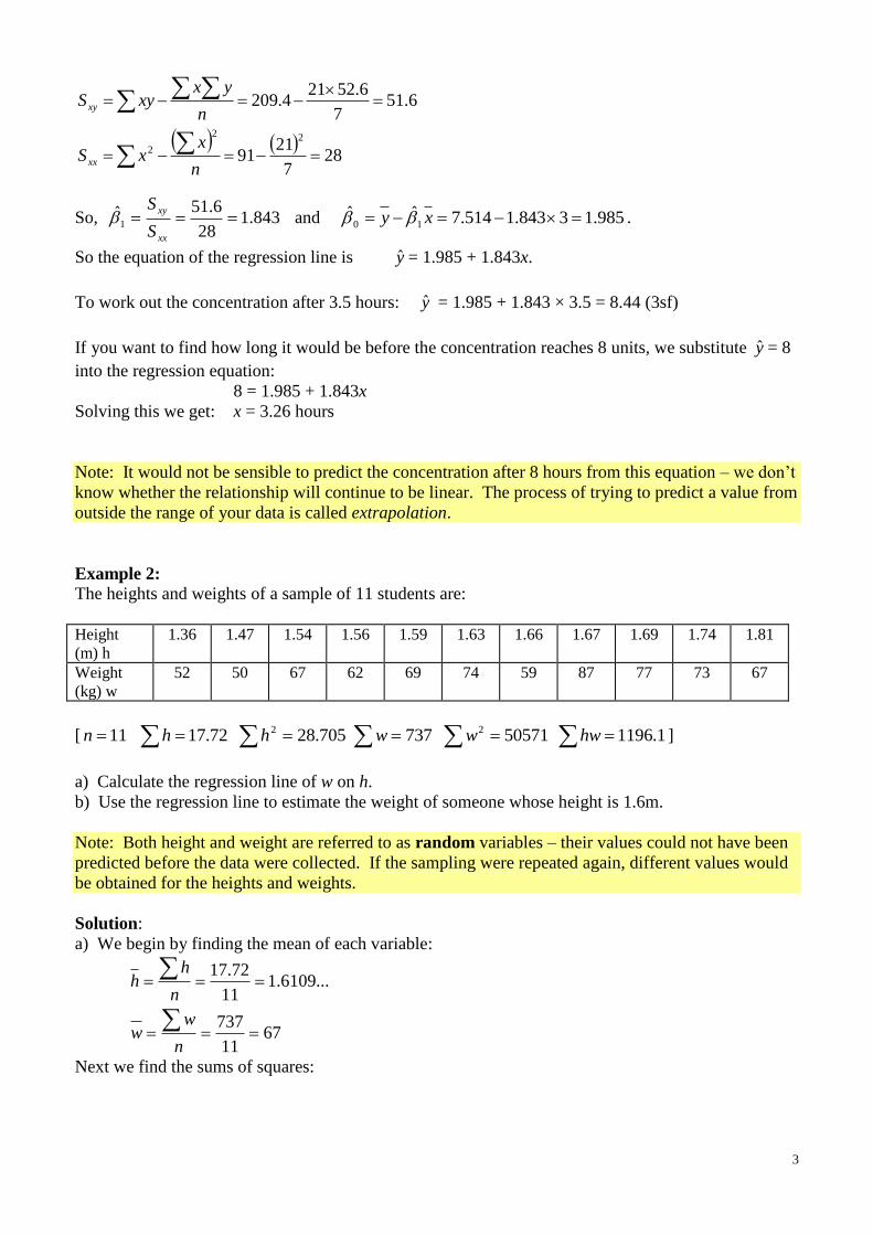
3

28

7

2191

6.517

6.52214.209

22

2

n

xxS

n

yxxyS

xx

xy

So, 843.128

6.51ˆ1

xx

xy

S

S and 985.13843.1514.7ˆˆ

10 xy .

So the equation of the regression line is y = 1.985 + 1.843x.

To work out the concentration after 3.5 hours: y = 1.985 + 1.843 × 3.5 = 8.44 (3sf)

If you want to find how long it would be before the concentration reaches 8 units, we substitute y = 8

into the regression equation:

8 = 1.985 + 1.843x

Solving this we get: x = 3.26 hours

Note: It would not be sensible to predict the concentration after 8 hours from this equation – we don’t

know whether the relationship will continue to be linear. The process of trying to predict a value from

outside the range of your data is called extrapolation.

Example 2: The heights and weights of a sample of 11 students are:

Height

(m) h

1.36 1.47 1.54 1.56 1.59 1.63 1.66 1.67 1.69 1.74 1.81

Weight

(kg) w

52 50 67 62 69 74 59 87 77 73 67

[ 1.119650571737705.2872.1711 22 hwwwhhn ]

a) Calculate the regression line of w on h.

b) Use the regression line to estimate the weight of someone whose height is 1.6m.

Note: Both height and weight are referred to as random variables – their values could not have been

predicted before the data were collected. If the sampling were repeated again, different values would

be obtained for the heights and weights.

Solution:

a) We begin by finding the mean of each variable:

6711

737

...6109.111

72.17

n

ww

n

hh

Next we find the sums of squares:

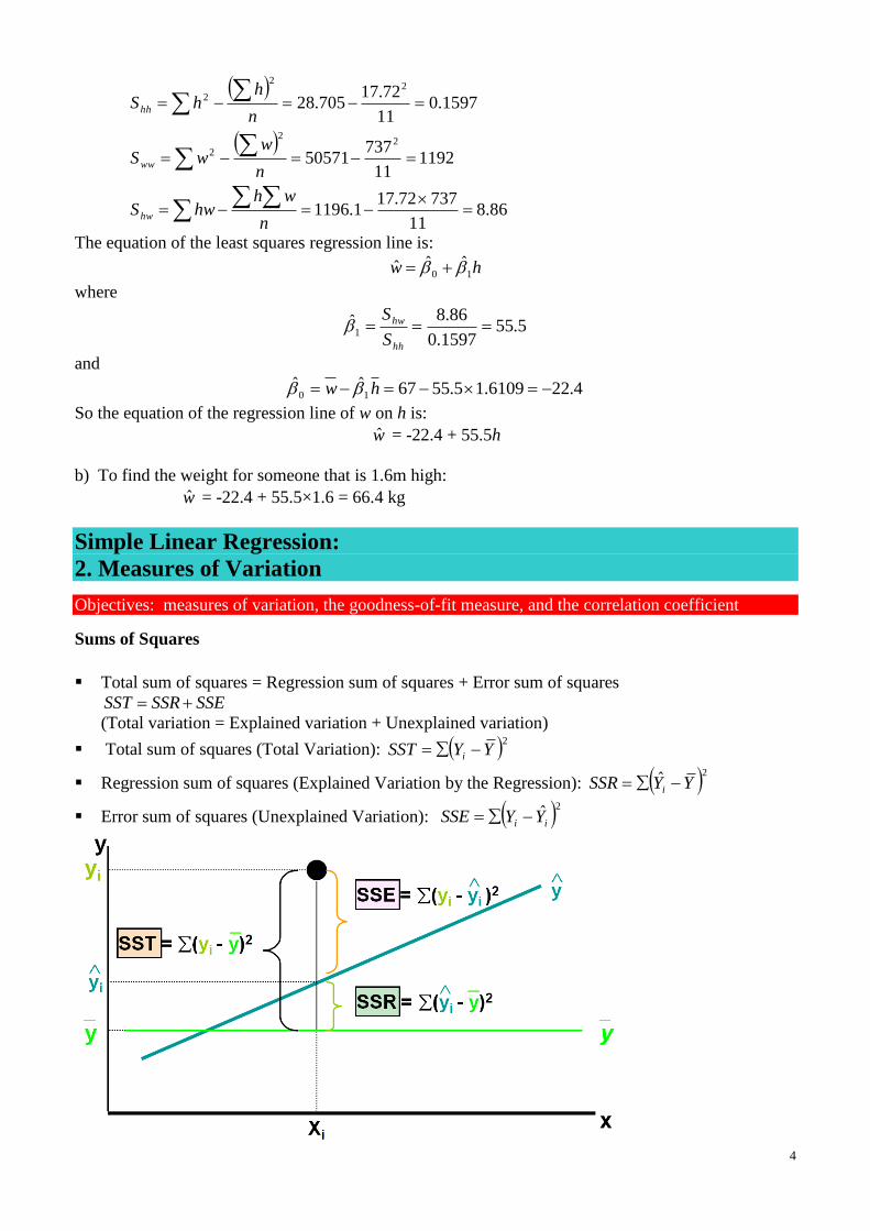
4

86.811

73772.171.1196

119211

73750571

1597.011

72.17705.28

22

2

22

2

n

whhwS

n

wwS

n

hhS

hw

ww

hh

The equation of the least squares regression line is:

hw 10ˆˆˆ

where

5.551597.0

86.8ˆ1

hh

hw

S

S

and

4.226109.15.5567ˆˆ10 hw

So the equation of the regression line of w on h is:

w = -22.4 + 55.5h

b) To find the weight for someone that is 1.6m high:

w = -22.4 + 55.5×1.6 = 66.4 kg

Simple Linear Regression:

2. Measures of Variation

Objectives: measures of variation, the goodness-of-fit measure, and the correlation coefficient

Sums of Squares

Total sum of squares = Regression sum of squares + Error sum of squares

SSESSRSST

(Total variation = Explained variation + Unexplained variation)

Total sum of squares (Total Variation): 2YYSST i

Regression sum of squares (Explained Variation by the Regression): 2ˆ YYSSR i

Error sum of squares (Unexplained Variation): 2ˆii YYSSE

5

Coefficients of Determination and Correlation

Coefficient of Determination – it is a measure of the regression goodness-of-fit

It also represents the proportion of variation in Y “explained” by the regression on X

SST

SSRR 2 ; 10 2 R

Pearson (Product-Moment) Correlation Coefficient -- measure of the direction and strength of

the linear association between Y and X

The sample correlation is denoted by r and is closely related to the coefficient of determination as

follows:

2

1ˆ Rsignr ; 11 r

The sample correlation is indeed defined by the following formula:

The corresponding population correlation between Y and X is denoted by ρ and defined by:

Therefore one can see that in the population correlation definition, both X and Y are assumed to

be random. When the joint distribution of X and Y is bivariate normal, one can perform the

following t-test to test whether the population correlation is zero:

• Hypotheses

H0: ρ = 0 (no correlation)

HA: ρ ≠ 0 (correlation exists)

• Test statistic

Note: One can show that this t-test is indeed the same t-test in testing the regression slope β1 = 0

shown in the following section.

Note: The sample correlation is not an unbiased estimator of the population correlation. You can

study this and other properties from the wiki site:

http://en.wikipedia.org/wiki/Pearson_product-moment_correlation_coefficient

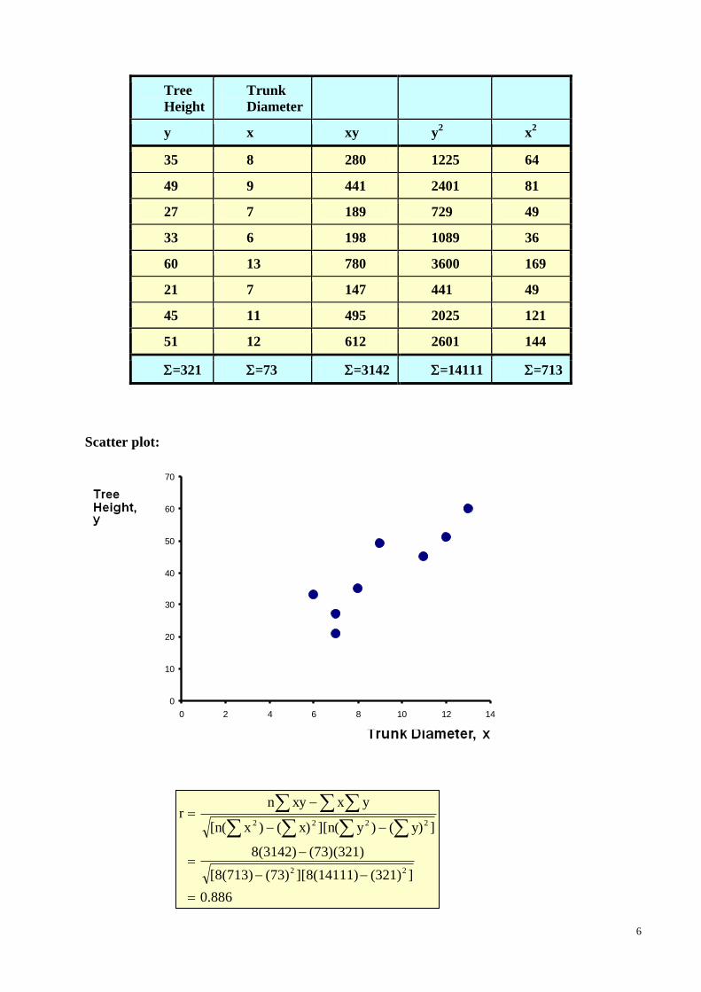
Example 3: The following example tabulates the relations between trunk diameter and tree height.

])()(][)()([])(][)([

))((

222222 yynxxn

yxxyn

SS

S

yyxx

yyxxr

YYXX

XY

YVarXVar

YYXXE

YVarXVar

YXCOV

,

22

0 ~0

2n

r1

rt

n

H

t

6

Tree

Height

Trunk

Diameter

y x xy y2 x

2

35 8 280 1225 64

49 9 441 2401 81

27 7 189 729 49

33 6 198 1089 36

60 13 780 3600 169

21 7 147 441 49

45 11 495 2025 121

51 12 612 2601 144

=321 =73 =3142 =14111 =713

Scatter plot:

0

10

20

30

40

50

60

70

0 2 4 6 8 10 12 14

0.886

](321)][8(14111)(73)[8(713)

(73)(321)8(3142)

]y)()y][n(x)()x[n(

yxxynr

22

2222

7

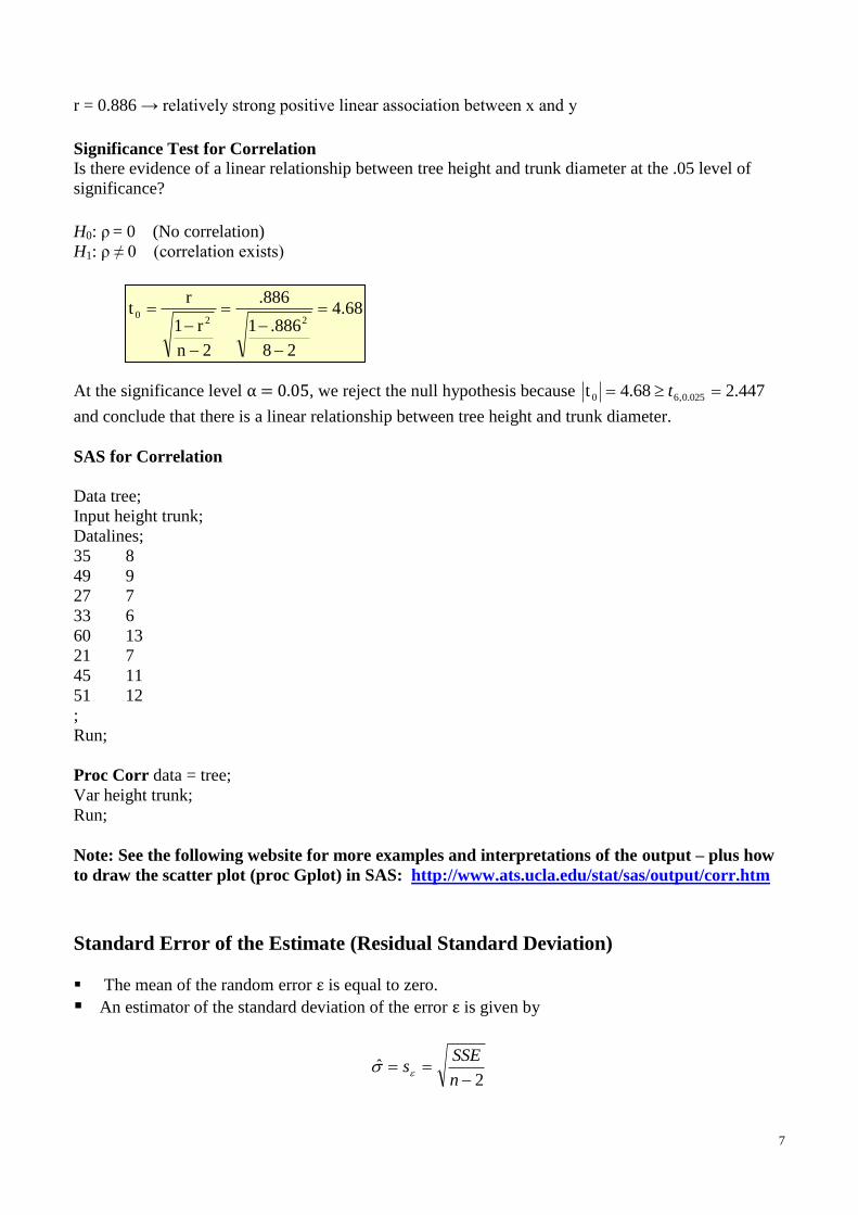
r = 0.886 → relatively strong positive linear association between x and y

Significance Test for Correlation

Is there evidence of a linear relationship between tree height and trunk diameter at the .05 level of

significance?

H0: ρ = 0 (No correlation)

H1: ρ ≠ 0 (correlation exists)

At the significance level α = 0.05, we reject the null hypothesis because 447.268.4t 025.0,60 t

and conclude that there is a linear relationship between tree height and trunk diameter.

SAS for Correlation

Data tree;

Input height trunk;

Datalines;

35 8

49 9

27 7

33 6

60 13

21 7

45 11

51 12

;

Run;

Proc Corr data = tree;

Var height trunk;

Run;

Note: See the following website for more examples and interpretations of the output – plus how

to draw the scatter plot (proc Gplot) in SAS: http://www.ats.ucla.edu/stat/sas/output/corr.htm

Standard Error of the Estimate (Residual Standard Deviation)

The mean of the random error ε is equal to zero.

An estimator of the standard deviation of the error ε is given by

2ˆ

n

SSEs

4.68

28

.8861

.886

2n

r1

rt

220

8

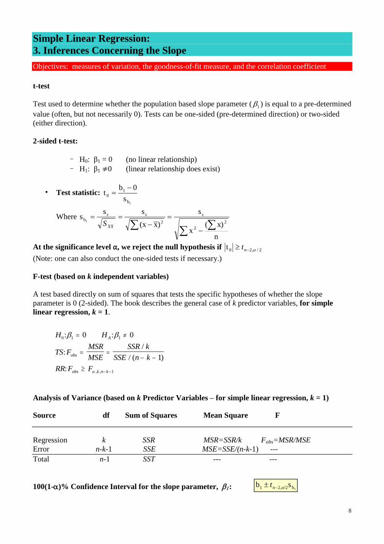
Simple Linear Regression:

3. Inferences Concerning the Slope

Objectives: measures of variation, the goodness-of-fit measure, and the correlation coefficient

t-test

Test used to determine whether the population based slope parameter ( 1 ) is equal to a pre-determined

value (often, but not necessarily 0). Tests can be one-sided (pre-determined direction) or two-sided

(either direction).

2-sided t-test:

– H0: β1 = 0 (no linear relationship)

– H1: β1 ≠0 (linear relationship does exist)

• Test statistic:

1b

10

s

0bt

Where

n

x)(x

s

)x(x

sss

2

2

ε

2

εε

b1

XXS

At the significance level α, we reject the null hypothesis if 2/,20t nt

(Note: one can also conduct the one-sided tests if necessary.)

F-test (based on k independent variables)

A test based directly on sum of squares that tests the specific hypotheses of whether the slope

parameter is 0 (2-sided). The book describes the general case of k predictor variables, for simple

linear regression, k = 1.

Analysis of Variance (based on k Predictor Variables – for simple linear regression, k = 1)

Source df Sum of Squares Mean Square F

Regression k SSR MSR=SSR/k Fobs=MSR/MSE

Error n-k-1 SSE MSE=SSE/(n-k-1) ---

Total n-1 SST --- ---

100(1-)% Confidence Interval for the slope parameter, :

H H

TS FMSR

MSE

SSR k

SSE n k

RR F F

A

obs

obs k n k

0 1 1

1

0 0

1

: :

:/

/ ( )

: , ,

1b/2,21 sb nt

9

If entire interval is positive, conclude >0 (Positive association)

If interval contains 0, conclude (do not reject) 0 (No association)

If entire interval is negative, conclude <0 (Negative association)

Example 4: A real estate agent wishes to examine the relationship between the selling price of a home

and its size (measured in square feet). A random sample of 10 houses is selected

– Dependent variable (y) = house price in $1000s

– Independent variable (x) = square feet

–

House Price in $1000s (y) Square Feet (x)

245 1400

312 1600

279 1700

308 1875

199 1100

219 1550

405 2350

324 2450

319 1425

255 1700

Solution: Regression analysis output:

Regression Statistics

Multiple R 0.76211

R Square 0.58082

Adjusted R

Square 0.52842

Standard Error 41.33032

Observations 10

ANOVAdf SS MS F

Significance

F

Regression 1 18934.9348

18934.934

8

11.084

8 0.01039

Residual 8 13665.5652 1708.1957

Total 9 32600.5000

Coefficien

ts Standard Error t Stat

P-

value Lower 95%

Upper

95%

Intercept 98.24833 58.03348 1.69296

0.1289

2 -35.57720

232.0738

6

Square Feet 0.10977 0.03297 3.32938

0.0103

9 0.03374 0.18580

10

• b1 measures the estimated change in the average value of Y as a result of a one-unit change in

X

– Here, b1 = .10977 tells us that the average value of a house increases by .10977($1000)

= $109.77, on average, for each additional one square foot of size

This means that 58.08% of the variation in house prices is explained by variation in square feet.

The standard error (estimated standard deviation of the random error) is also given in the output

(above).

• t test for a population slope

– Is there a linear relationship between x and y?

• Null and alternative hypotheses

– H0: β1 = 0 (no linear relationship)

– H1: β1 ≠ 0 (linear relationship does exist)

• Test statistic:

–

At the significance level α = 0.05, we reject the null hypothesis because

306.2329.3t 025.0,80 t and conclude that there is sufficient evidence that square footage affects

house price.

Confidence Interval Estimate of the Slope:

The 95% confidence interval for the slope is (0.0337, 0.1858)

Since the units of the house price variable is $1000s, we are 95% confident that the average impact on

sales price is between $33.70 and $185.80 per square foot of house size

This 95% confidence interval does not include 0.

Conclusion: There is a significant relationship between house price and square feet at the .05 level of

significance

Predict the price for a house with 2000 square feet:

feet) (square 0.10977 98.24833 price house Estimated

0.5808232600.5000

18934.9348

SST

SSRR 2

41.33032sε

329.3s

0bt

1b

10

1b/2,21 sb nt

317.85

0)0.1098(200 98.25

(sq.ft.) 0.1098 98.25 price house

11

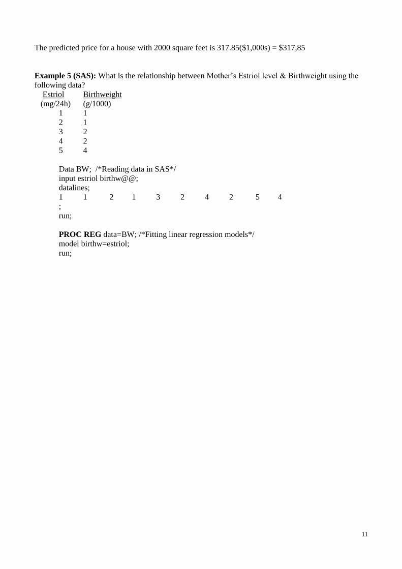
The predicted price for a house with 2000 square feet is 317.85($1,000s) = $317,85

Example 5 (SAS): What is the relationship between Mother’s Estriol level & Birthweight using the

following data?

Estriol Birthweight

(mg/24h) (g/1000)

1 1

2 1

3 2

4 2

5 4

Data BW; /*Reading data in SAS*/

input estriol birthw@@;

datalines;

1 1 2 1 3 2 4 2 5 4

;

run;

PROC REG data=BW; /*Fitting linear regression models*/

model birthw=estriol;

run;

12

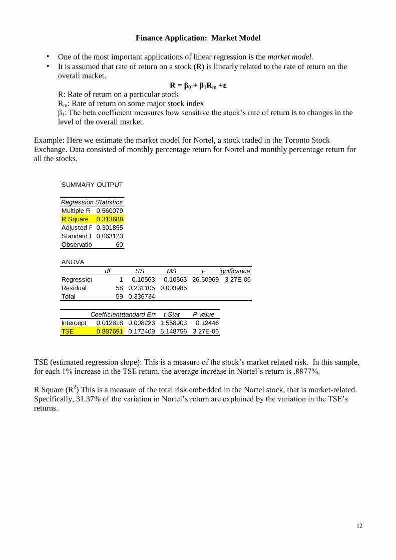
Finance Application: Market Model

• One of the most important applications of linear regression is the market model.

• It is assumed that rate of return on a stock (R) is linearly related to the rate of return on the

overall market.

R = β0 + β1Rm +ε

R: Rate of return on a particular stock

Rm: Rate of return on some major stock index

β1: The beta coefficient measures how sensitive the stock’s rate of return is to changes in the

level of the overall market.

Example: Here we estimate the market model for Nortel, a stock traded in the Toronto Stock

Exchange. Data consisted of monthly percentage return for Nortel and monthly percentage return for

all the stocks.

TSE (estimated regression slope): This is a measure of the stock’s market related risk. In this sample,

for each 1% increase in the TSE return, the average increase in Nortel’s return is .8877%.

R Square (R2) This is a measure of the total risk embedded in the Nortel stock, that is market-related.

Specifically, 31.37% of the variation in Nortel’s return are explained by the variation in the TSE’s

returns.

SUMMARY OUTPUT

Regression Statistics

Multiple R 0.560079

R Square 0.313688

Adjusted R Square0.301855

Standard Error0.063123

Observations 60

ANOVA

df SS MS F Significance F

Regression 1 0.10563 0.10563 26.50969 3.27E-06

Residual 58 0.231105 0.003985

Total 59 0.336734

CoefficientsStandard Error t Stat P-value

Intercept 0.012818 0.008223 1.558903 0.12446

TSE 0.887691 0.172409 5.148756 3.27E-06

13

Linear Regression in Matrix Form

Data:

).,,,,(,),,,,,(),,,,,( 12112222121112111 npnnnpp xxxyxxxyxxxy

The multiple linear regression model in scalar form is

.,,1),,0(~, 2

1122110 niNxxxy iiippiii

The above linear regression can also be represented in the vector/matrix form. Let

1

2

0

2

1

11

1221

1111

2

1

,,

1

1

1

,

pnnpn

p

p

nxx

xx

xx

X

y

y

y

βεy .

Then,

nnppn

pp

pp

nnppn

pp

pp

nxx

xx

xx

xx

xx

xx

y

y

y

2

1

11110

1212110

1111110

11110

21212110

11111110

2

1

y

= εXβ

npnpn

p

p

xx

xx

xx

2

1

1

1

0

11

1221

1111

1

1

1

.

Estimation: Least square method: The least square method is to find the estimate of β minimizing the sum of square of residual,

εεβ t

n

n

n

i

ipSS

2

1

21

1

2

110 ),,,()(

)()( XβyXβy t

since XβYε . Expanding )(βS yields

))(()()()( XβyXβyXβyXβyβ ttt tS

XβXβyX2βyy

XβXβyXβXβyyy

ttttt

tttttt

Note:

For two matrices A and B, tttABAB and 11 tt

AA

Similar to the procedure in finding the minimum of a function in calculus, the least square estimate b

can be found by solving the equation based on the first derivative of )(βS ,

14

0Xβ2Xy2X

β

XβXβyX2βyy

β

β

β

β

β ttttttt

1

1

0

)(

p

S

S

S

S

yXXβX tt

1

1

0

pb

b

b

yXX)(Xb t1t

The fitted regression equation is

1122110ˆ

pp xbxbxbby .

The fitted values (in vector):

ny

y

y

ˆ

ˆ

ˆ

ˆ 2

1

Xby

The residuals (in vector):

ne

e

e

2

1

ˆ eXbyyy

Note: (i) ,

)()( 1

1

aββ

aβ t

p

i

ii a

where

1

1

0

p

β and

pa

a

a

2

1

a .

(ii) ,2

)()( 1 1

11

Aβββ

Aββ t

p

i

p

j

ijji a

where A is any symmetric pp matrix.

Note: Since

XXXXXX tttttt ,

XX t is a symmetric matrix.

Also,

111 XXXXXX ttt

tt ,

1XX t is a symmetric matrix.

Note: YXXβX tt is called the normal equation.

Note: XXX)X(XyXyXXX)X(Xyy)XXb(yXe t1tttt1ttttttt

0XyXy tt .

15

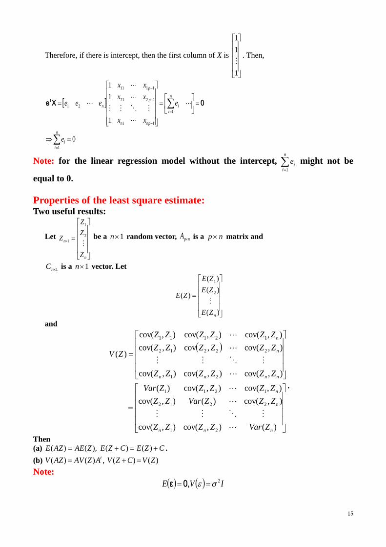
Therefore, if there is intercept, then the first column of X is

1

1

1

. Then,

0

1

1

1

1

1

11

1221

1111

21

n

i

i

n

i

i

npn

p

p

n

e

e

xx

xx

xx

eee 0Xe t

Note: for the linear regression model without the intercept,

n

i

ie1

might not be

equal to 0.

Properties of the least square estimate: Two useful results:

Let

n

n

Z

Z

Z

Z

2

1

1 be a 1n random vector, npA is a np matrix and

1nC is a 1n vector. Let

)(

)(

)(

)(2

1

nZE

ZE

ZE

ZE

and

)(),cov(),cov(

),cov()(),cov(

),cov(),cov()(

),cov(),cov(),cov(

),cov(,cov),cov(

),cov(),cov(),cov(

)(

21

2212

1211

21

22212

12111

nnn

n

n

nnnn

n

n

ZVarZZZZ

ZZZVarZZ

ZZZZZVar

ZZZZZZ

ZZZZZZ

ZZZZZZ

ZV

.

Then

(a) CZECZEZAEAZE )()( ),()( .

(b) )()( ,)()( ZVCZVAZAVAZV t

Note:

IVE 2, 0ε

16

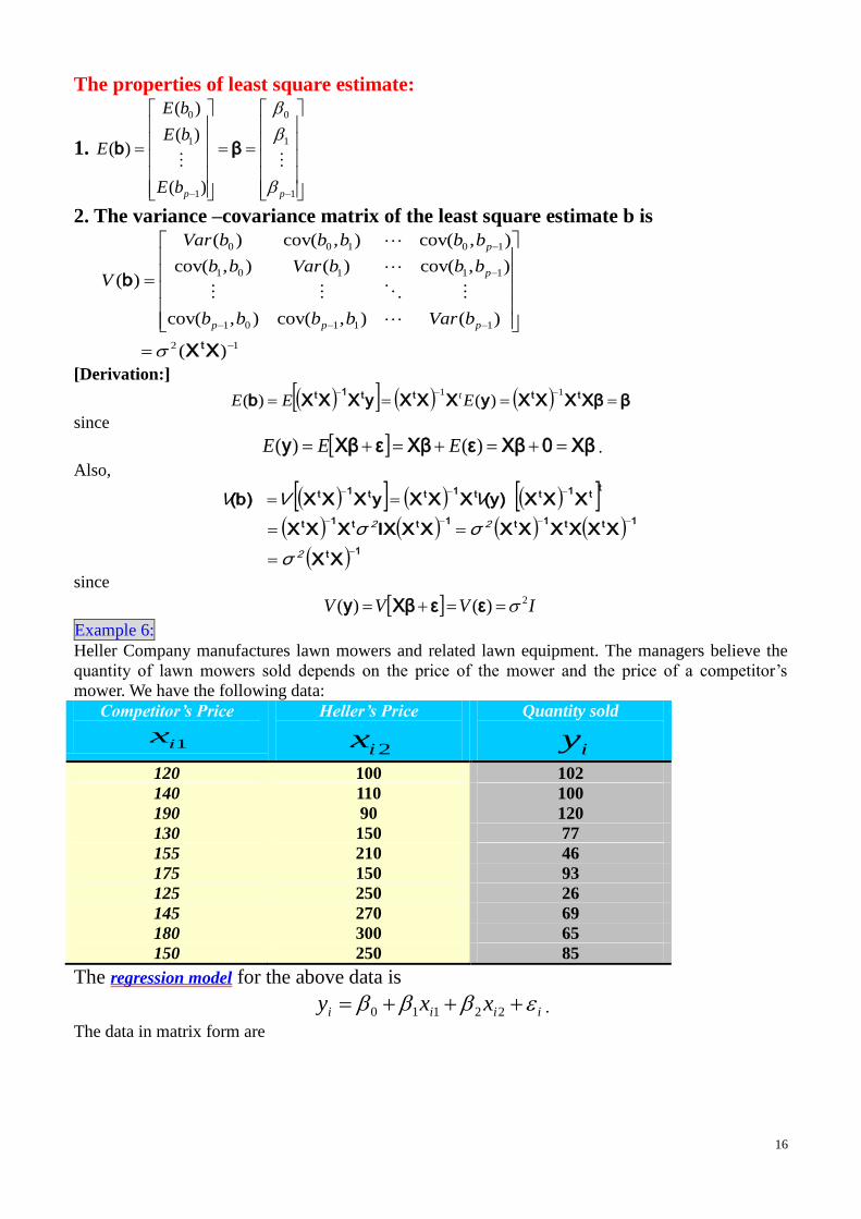
The properties of least square estimate:

1.

1

1

0

1

1

0

)(

)(

)(

)(

ppbE

bE

bE

E

βb

2. The variance –covariance matrix of the least square estimate b is

12

11101

11101

10100

)(

)(),cov(),cov(

),cov()(),cov(

),cov(),cov()(

)(

XX

b

t

ppp

p

p

bVarbbbb

bbbVarbb

bbbbbVar

V

[Derivation:]

βXβXXXyXXXyXXXb tttt1t 11

)()( EEE t

since

Xβ0XβεXβεXβy )()( EEE .

Also,

1t

1tt1t1tt1t

tt1tt1tt1t

XX

XXXXXXXXIXXXX

XXX(y)XXXyXXX(b)

2

22

σ

σσ

VVV

since

IVVV 2)()( εεXβy

Example 6:

Heller Company manufactures lawn mowers and related lawn equipment. The managers believe the

quantity of lawn mowers sold depends on the price of the mower and the price of a competitor’s

mower. We have the following data:

Competitor’s Price

1ix

Heller’s Price

2ix

Quantity sold

iy

120 100 102

140 110 100

190 90 120

130 150 77

155 210 46

175 150 93

125 250 26

145 270 69

180 300 65

150 250 85

The regression model for the above data is

iiii xxy 22110 .

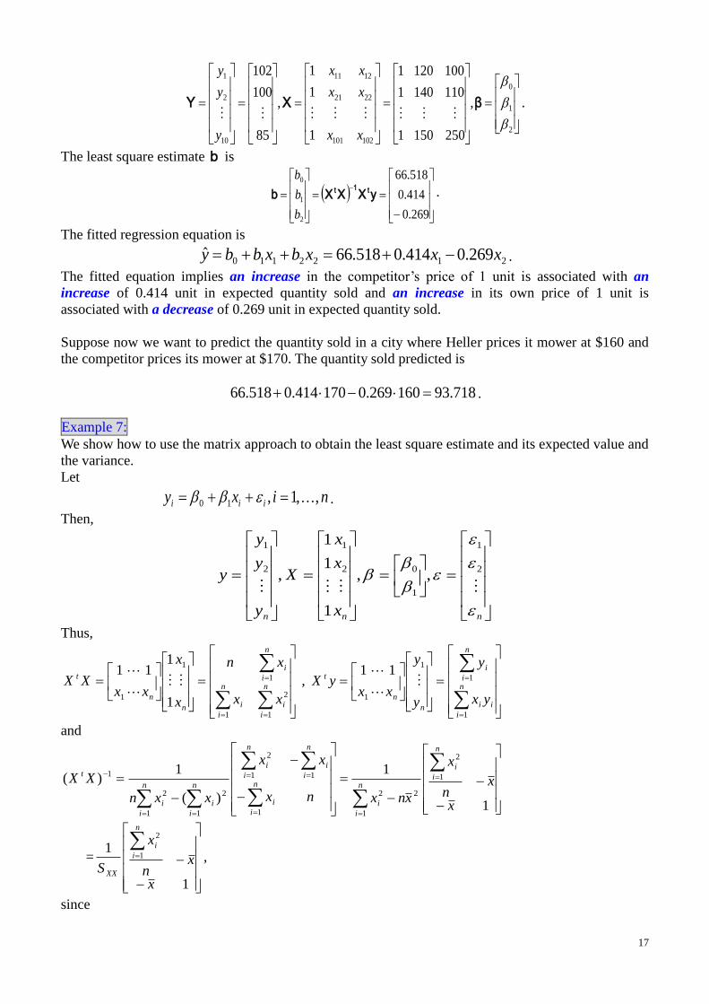
The data in matrix form are

17

2

1

0

102101

2221

1211

10

2

1

,

2501501

1101401

1001201

1

1

1

,

85

100

102

βXY

xx

xx

xx

y

y

y

.

The least square estimate b is

269.0

414.0

518.66

2

1

0

yXXXb t1t

b

b

b

.

The fitted regression equation is

2122110 269.0414.0518.66ˆ xxxbxbby .

The fitted equation implies an increase in the competitor’s price of 1 unit is associated with an

increase of 0.414 unit in expected quantity sold and an increase in its own price of 1 unit is

associated with a decrease of 0.269 unit in expected quantity sold.

Suppose now we want to predict the quantity sold in a city where Heller prices it mower at $160 and

the competitor prices its mower at $170. The quantity sold predicted is

718.93160269.0170414.0518.66 .

Example 7:

We show how to use the matrix approach to obtain the least square estimate and its expected value and

the variance.

Let

nixy iii ,,1,10 .

Then,

nnn x

x

x

X

y

y

y

y

2

1

1

02

1

2

1

,,

1

1

1

,

Thus,

n

i

i

n

i

i

n

i

i

n

n

t

xx

xn

x

x

xxXX

1

2

1

1

1

11

111

,

n

i

ii

n

i

i

n

n

t

yx

y

y

y

xxyX

1

1

1

1

11

and

1

1

)(

1)( 1

2

2

1

2

1

11

2

1

2

1

2

1

x

xn

x

xnxnx

xx

xxn

XX

n

i

i

n

i

i

n

i

i

n

i

i

n

i

i

n

i

i

n

i

i

t

=

1

11

2

x

xn

x

S

n

i

i

XX

,

since

18

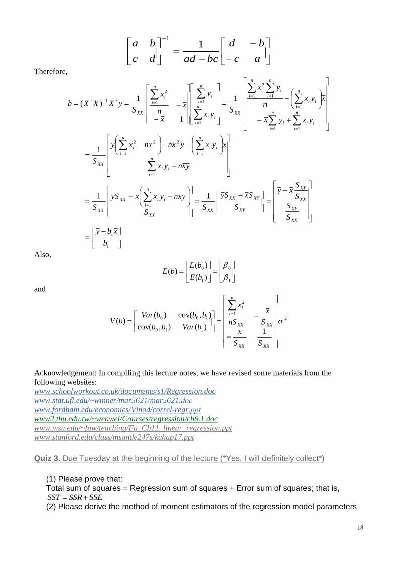
ac

bd

bcaddc

ba 11

Therefore,

n

i

ii

n

i

i

n

i

ii

n

i

i

n

i

i

XX

n

i

ii

n

i

i

n

i

i

XX

tt

yxyx

xyxn

yx

Syx

y

x

xn

x

SyXXXb

11

1

11

2

1

11

2

1 1

1

1)(

1

1

1

1

1

22

1

2

11

1

b

xby

S

S

S

Sxy

S

SxSy

SS

yxnyxxSy

S

yxnyx

xyxyxnxnxy

S

XX

XY

XX

XY

XY

XYXX

XXXY

n

i

iiXX

XX

n

i

ii

i

n

i

i

n

i

i

XX

Also,

1

0

1

0

)(

)()(

bE

bEbE

and

21

2

110

100

1)(),cov(

),cov()()(

XXXX

XXXX

n

i

i

SS

x

S

x

nS

x

bVarbb

bbbVarbV

Acknowledgement: In compiling this lecture notes, we have revised some materials from the

following websites:

www.schoolworkout.co.uk/documents/s1/Regression.doc

www.stat.ufl.edu/~winner/mar5621/mar5621

www.fordham.edu/economics/Vinod/correl-regr.

www2.thu.edu.tw/~wenwei/Courses/regression/ch6.1.doc

www.msu.edu/~fuw/teaching/Fu_Ch11_linear_regression.ppt

www.stanford.edu/class/msande247s/kchap17.ppt

Quiz 3. Due Tuesday at the beginning of the lecture (*Yes, I will definitely collect*)

(1) Please prove that: Total sum of squares = Regression sum of squares + Error sum of squares; that is,

SSESSRSST

(2) Please derive the method of moment estimators of the regression model parameters