REGIONAL EFFECTS OF MONETARY POLICY IN …web.usm.my/aamj/19012014/Art 6 (113-146).pdf · The Literature in Other Countries When discussing the regional effects of monetary policy,

Asian Academy of Management Journal, Vol. 19, No. 1, 113–146, 2014

© Asian Academy of Management and Penerbit Universiti Sains Malaysia, 2014

REGIONAL EFFECTS OF MONETARY POLICY IN CHINA: THE ROLE OF SPILLOVER EFFECTS

Guo Xiaohui1* and Tajul Ariffin Masron2

1 School of Economics, Hebei University, Baoding, 071002 China 1,2 School of Management, Universiti Sains Malaysia 11800 USM Pulau Pinang

*Corresponding author: [email protected]

ABSTRACT

This paper uses Structural Vector Autoregressive (SVAR) method to measure the regional effects of monetary policy in China during 1978–2011. The results provide evidence of different regional responses of real variables to monetary policy shocks. This paper proves that M2 is a better monetary policy indicator. We also find that when examining the regional effects of monetary policy in China, the spillover effects among regions are very important in the short run. In the long run, the influence of deposits transfer among regions is much bigger than that of the spillover effects.

Keywords: Monetary policy, structural vector autoregressive, spillover effects

INTRODUCTION

China's economy is huge and expanding rapidly. The growth of China's economy since the initiation of economic reform and opening up in 1978 has been one of the wonders of modern economic development. China has experienced unprecedented economic growth in the past thirty years, with GDP rising on average by almost 9.9% per annum from 1978 until 2011. Indeed, China overtook Japan and became the world's second largest GDP measured in US dollars in 2010.

Monetary policy has played an important role in China's fast-growing economy since 1978 (Hsing & Hsieh, 2004; Dickinson & Liu, 2007; He, Leung, & Chong, 2013). However, the conduct of monetary policy by the People's Bank of China (PBC, the central bank of China) depends primarily on the real economic conditions of the country as a whole without considering regional economic differences. China is a vast country with significant regional disparity. Given its size and geography, China can be divided into three regions: the developed eastern region and the less-developed middle and western regions1. Figure 1 shows that the output gap among the three regions has been widening since 1992. This notion of growing disparity in China is also supported by previous studies,

Guo Xiaohui and Tajul Ariffin Masron

114

including Pedroni and Yao (2006), Lau (2010) and Fan, Kanbur and Zhang (2011), among others.

Figure 1. The GDP per capita of the three regions (Unit: CNY) Data source: National Bureau of Statistics of China

In reality, diverse regions within a large country that have different structures may respond differently to changing economic circumstances. Thus, monetary policy may have varied influences on different regions (Carlino & DeFina, 1998). Therefore, China's common monetary policy may have different effects across different regions in China. Moreover, the varied effects of monetary policy may exacerbate existing regional disparities.

As we know, monetary policy will eventually affect regional economies through monetary transmission channels. However, this is far from the culmination of potential economic effects because different regions interact with each other through interregional links. For example, the earthquake that struck the Sichuan province of China in 2008 and caused substantial damage to the Sichuan economy initially affected only the output of Sichuan. However, it is possible that the economic shock caused by the earthquake eventually produced economic effects on nearby provinces, such as Gansu, Qinghai and Shaanxi. Such effects are called spillover effects. Therefore, monetary policy may have two distinct effects on each region: a direct effect via monetary transmission channels and an indirect effect produced by spillover effects among regions (see Figure 2). To our knowledge, the previous literature that examines the regional effects of monetary policy in China (such as Cortes & Kong, 2007) neglects to consider spillover effects. Thus, this study conducts an examination of the regional effects of China's monetary policy that accounts for spillover effects.

Regional Effects of Monetary Policy in China

115

Figure 2. Direct and indirect effects of monetary policy on regions LITERATURE REVIEW

The Literature in Other Countries

When discussing the regional effects of monetary policy, we use the Theory of Optimum Currency Area (OCA) as the theoretical basis. The OCA theory was introduced by Mundell (1961), who argued that a currency area should be a region whose borders need not necessarily coincide with state borders. The borders of an OCA may be beyond or within the borders of a state. For large countries with substantial disparities among regional economies, such as China, whether OCA standards are met would exert a significant influence on the effects of monetary policy. Therefore, many scholars (Beare, 1976; Cohen & Maeshiro, 1977; Fishkind, 1977; Garrison & Chang, 1979) have started to pay attention to the different regional effects of monetary policy within a single country. Empirical studies (Carlino & DeFina, 1998; 1999; Weber, 2006; Cortes & Kong, 2007; Georgopoulos, 2009) indicate that a common monetary policy does indeed exert varied regional effects in large countries, such as the United States, China, Canada and Australia.

Beare (1976) notes that money contributes to fluctuations in the activity levels of different regions of a national economy and uses a St. Louis reduced-form model to test the monetarist's view that business cycles are due primarily to monetary shocks at the regional level. The results suggest the importance of money in the determination of regional activity levels in the short run. Following Beare (1976), many other scholars (Cohen & Maeshiro, 1977; Mathur & Stein, 1983; Garrison

Monetary Policy

Region A

Region B

Monetary transmission Channel

The Spillover Effects

Direct Effect

Direct Effect

Indirect Effect


116

& Kort, 1983; Garrison & Chang, 1979) also examine the monetarist proposition that monetary policy has a significant impact on nominal income at the regional level.

The pioneering use of VAR models to estimate regional asymmetric reactions to shocks can be found in Carlino and DeFina (1998; 1999). Carlino and DeFina first apply the VAR method to study the differential regional effects of monetary policy in the United States and find that impulse response functions show that not all regions respond by the same magnitude. Carlino and DeFina (1998; 1999) also summarise three possible reasons why the Federal Reserve System (Fed) policy actions might have differential regional effects: different regional structures of interest-sensitive industries, regional differences in the mix of large and small firms, and differences in regions' reliance on small (versus large) banks. However, their findings only confirm the transmission of monetary policy through the interest rate channel. They find no evidence that a credit channel for monetary policy operates at the regional level.

De Lucio and Izquierdo (1999) use quarterly data for Spanish regions from 1978:01 to 1998:01 to study the different regional effects of a common monetary policy and the local characteristics that underlie these differential responses. They estimate a SVAR model for each Spanish region using SUR techniques to characterise regional responses. The results suggest that different Spanish regions react differently to a common monetary policy, similar to the results obtained by Carlino and DeFina (1999) for the U.S.

Since Carlino and DeFina (1998; 1999)'s pioneering work, many scholars have applied the VAR method to examine the regional effects of monetary policy in their own countries. Weber (2006) focuses on Australia, Nachane, Ray and Ghosh (2002) apply the VAR method in India, Cortes and Kong (2007) apply it China and Georgopoulos (2009) applies it in Canada. All of these studies confirm the existence of regional effects of monetary policy in their respective countries.

The Literature in China

Scholars started to pay attention to the regional effects of monetary policy in China from the quantitative perspective during the past 10 years. Most of these studies adopt the VAR method.

Kong et al. (2007) (in Chinese) use the VAR method to study the influences of monetary policy on real output in China as a whole and in 29 individual provinces (Tibet and Chongqing were not included in the study) from 1980 to 2005. Their VAR system uses five variables: M2, real effective exchange rate,


117

GDP deflator, provincial GDP and an exogenous variable, world output. They test the VAR model province by province and their results confirm the previous findings. Cortes and Kong (2007) measure the impact of monetary policy on real output in China and its individual provinces during 1980–2004 period using the Vector Error Correction (VEC) method. They develop a provincial GDP system comprising four endogenous variables (a monetary policy variable (M2 or bank lending rate), exchange rate, price index and provincial real GDP) and one exogenous variable, world GDP. Using VEC-generated impulse response functions, they find that monetary shocks produce greater responses in coastal provinces than in inland provinces.

Jiang and Chen (2009) (in Chinese) employ the SVAR method to examine this issue. Their regional SVAR system contains M2, real regional GDP, loans of financial institutions and a GDP deflator from 1978 to 2006. The difference is that they divide China into the eight regions defined in "The Strategy and Policy of Coordinated Regional Development" published by the Development Research Center of the State Council. They find that regions with higher productivity levels are more sensitive to monetary policy shocks.

One shortcoming of these studies is that they attempt to measure monetary policy impacts region by region (province by province) without accounting for spillover effects among regions. Ying (2000), Brun, Combes and Renald (2002), and Groenewold, Lee and Chen (2007) examine the spillover effects of output among the three regions and different provinces. They find that strong spillovers exist from the coastal region to the other two regions and from the Middle region to the western region. Thus, in this study, we will examine the regional effects of monetary policy accounting for spillover effects. Furthermore, we will compare the regional effects of monetary policy with and without spillover effects in order to check the significance of spillover effects.

METHODOLOGY

Model Specification

Following Carlino and DeFina (1998; 1999), we use the SVAR model to measure the regional effects of monetary policy in China. The advantage of the VAR model is that it does not rely on any economic theory. The specification of our SVAR model is as follows:


118

0 3 4

5 6 1

1 2i t i i t i i t i i t i

i t i t

k k k kt 1 =1 =1 =1 =1

k=1

c EGDP + Price MP EGDP MGDP

WGDP WDGDP e

α α α α α

α α− − − −

−

= ∑ ∑ ∑ ∑

∑

+ + + +

+ + (1)

0 1 2 3 4

5 6 2

k k k k2 i t i i t i i t i i t i

ki t i t

t =1 =1 =1 =1

=1

c MGDP Price MP EGDP MGDP

WGDP WDGDP e

β β β β β

β β− − − −

−

= + + + + +

+ +

∑ ∑ ∑ ∑∑

(2)

3 0 1 2 3 4

5 6 3

k k k ki t i i t i i t i i t i

ki t i t

t =1 =1 =1 =1

=1

c WGDP y Price MP EGDP MGDP

WGDP WDGDP e

γ γ γ γ

γ γ

− − − −

−

= + + + + +

+ +

∑ ∑ ∑ ∑∑

(3)

0 1 2 3 4

5 6 4

Pr k k k k4 t i t i i t i i t i i t i

ki t i t

=1 =1 =1 =1

=1

c ice a a Price a MP a EGDP a MGDP

a WGDP a WDGDP e− − − −

−

= + + + + +

+ +

∑ ∑ ∑ ∑∑

(4)

5 0 1 2 3 4

5 6 5

k k k ki t i i t i i t i i t i

ki t i t

=1 =1 =1 =1

=1

c MP b b Price b MP b EGDP b MGDP

b WGDP b WDGDP e− − − −

−

= + + + + +

+ +

∑ ∑ ∑ ∑∑

(5)

MP is the monetary policy variable (measured by M2, M1 or the one-year bank lending rate). Price is the national price level measured by the CPI index. EGDP, MGDP and WGDP are the real GDPs of the East, Middle and West, respectively. WDGDP is real World GDP, an exogenous variable. This SVAR system treats these variables (except WDGDP) as endogenous. It relies on these variables expressed as past values of the dependent variable and past values of the other variables in the model. We can estimate this SVAR model to analyse the system's responses to monetary policy shocks. The shock is the positive residual of one standard deviation unit in the monetary policy equation of the system.

We can express (1)–(5) in the form of vector Yt, where

Then, we get

1Y = [EGDP WGDP Prince MP ]t t t t t, , ,

( )CY = A(L)Y H L WDGDP ut t tt 1 + +− (6)


119

Where C is a 5 × 5 matrix of coefficients describing the contemporaneous correlation among the variables; A(L) and H(L) are 5 × 5 matrices of polynomials in the lag operator; and ut is a 5 × 1 vector of structural residuals. We will use annual data to estimate the model during 1978–2011.

1U [U U U U U ]t pt, mt,1t, 2t, 3t,− To see this more explicitly, we rewrite (6) as a reduced-form VAR:

( )Y = Z(L)Y G L WDGDP et t tt + +−1 (7)

where Z(L) = C–1A(L) and G(L) = C–1H(L) are infinite-order lag polynomials, and et = C-1ut and ut = Cet describe the relationship between the model's reduced-form residuals and the model's structural residuals. We can transform ut = Cet into an A-B SVAR specification in order to estimate the model: Aet = But. The problem of identifying the structural shocks ut from the VAR reduced-form residuals et and their variances will be discussed later. The solution depends on identification restrictions placed on the A and B matrices and on the variance-covariance matrix of structural errors.

Variable Selection

In our SVAR system, there are five endogenous variables: EGDP, MGDP, WGDP, Price and MP, and one exogenous variable, WDGDP. The estimating period is 1978–2011. EGDP, MGDP and WGDP are real regional GDPs in the East, Middle and West, respectively. These three variables measure regional-level economic activity. Price is the national price level measured by CPI (Consumer Price Index, 1978 = 100). The VAR model has been plagued by the price puzzle2 (Sims, 1992). Sims (1992) suggests that the price puzzle might be because interest rate innovations partially reflect inflationary pressures that lead to price increases. We include the price level in our model to examine the effects of monetary policy on inflation and the price puzzle. The exogenous variable WDGDP is included to isolate exogenous economic changes. China is an opening country, and foreign trade and FDI both provide momentum for China's economic growth. In recent years, China's economy has become more and more sensitive the world economy (Zhang & Zhang, 2003). Therefore, we add real world GDP as an exogenous variable in our SVAR system.


120

MP is the monetary policy variable. An important issue that arises in the analysis of regional effects of monetary policy is how to measure the stance of monetary policy. Bernanke and Blinder (1992) note that the Federal funds rate is a good indicator of monetary policy actions and suggest using innovations to the funds rate as a measure of changes in monetary policy. In China, all benchmark interest rates are regulated by the PBC. Because China is a transitioning country, interest rate liberalisation is in process; however, changes to the interest rate may not precisely reflect the supply and demand of funds. Monetary aggregates also are not ideal indicators of monetary policy because they are subject to a wide variety of disturbances, including shifts in the demand for money, which often dominate the information contained in monetary aggregates about changes in policy. In addition, Sun (2013) indicates that in China, M2 is also influenced by the PBC's foreign exchange purchases. Accordingly, these two variables are not the best measures of monetary policy in China. However because our estimation covers the period from the initiation of economic reform in 1978 until 2011, there are no other variables that are better monetary policy indicators than these two.

Previous studies, such as Song and Zhong (2006), Kong et al. (2007) and Cortes and Kong (2007), adopt M2 as the monetary policy variable. Cortes and Kong (2007) also use the bank lending rate as an indicator of monetary policy actions. In China, the one-year deposit and loan rates are the benchmark interest rates regulated by the PBC as monetary policy instruments. Kong et al. (2007) use a VAR model to measure the influence of monetary policy, represented by M2 or the bank lending rate, on the real economy. The results show that the influence of M2 is greater than the bank lending rate, so they conclude that M2 is better than the bank lending rate as a monetary policy variable. To demonstrate the robustness of the results of our SVAR model, we first use M2 as the monetary policy variable and then use M1 and the one-year bank lending rate as monetary policy variables to compare the results. The annual data for China during 1978–2011 are taken from the National Bureau of Statistics of China and the Almanac of China's Finance and Banking (1986–2012).

The Identification Problem

A widely recognised problem with SVAR is that the results are sensitive to the model's identification scheme (Sims & Zha, 1995). Thus, seemingly small changes in the identifying assumptions can lead to substantial changes in the estimated effects of the shocks and in their relative importance over the sample period. This sensitivity has led many researchers to test the results informally against over-identifying restrictions. A popular restriction used to identify monetary policy shocks and advocated by Bernanke and Blinder (1992) is that monetary policy has no instantaneous impact on output and inflation. This


121

assumption is appealing, given the broadly held view that the effects of monetary policy are not felt for a considerable time. Moreover, Fan, Yu and Zhang (2011) prove that the formulation of China's monetary policy follows the Taylor and McCallum rules3. Therefore, in this study, we adopt the restriction suggested by Bernanke and Blinder (1992). For the AB-SVAR model Aet = But, our first SVAR ordering of the five endogenous variables is EGDP, MGDP, WGDP, Price, MP. The identification matrices A and B are as follows:

A =

1 0 0 0 0

(8) a21 1 0 0 0 a31 a32 1 0 0 a41 a42 a43 1 0 a51 a52 a53 a54 1

B =

b11 0 0 0 0

(9) 0 b22 0 0 0 0 0 b33 0 0 0 0 0 b44 0 0 0 0 0 b55

Matrix A reflects the contemporaneous relationship of the five endogenous variables. We assume that monetary policy has no instantaneous impact on EGDP, MGDP, WGDP and Price. Within one period, EGDP can affect MGDP and WGDP and MGDP can affect WGDP, but MGDP and WGDP cannot affect EGDP and WGDP cannot affect MGDP (Groenewold, Lee, & Chen, 2007). Because the East is significantly more developed than the Middle and West, this assumption is in line with reality. We also assume that the structural residuals have unit variances; thus, we treat matrix B as a diagonal matrix. The elements in the main diagonal are simply the estimated standard deviations of the structural shocks.

In our first SVAR ordering of endogenous variables, we adopt the assumptions that monetary policy has no instantaneous impact on output and inflation and that the PBC formulates monetary policy based on the inflation and output gaps. Thus, the monetary policy variable ranks last in our first identification scheme. However, as Di Giacinto (2003) suggests, this assumption is likely to be too


122

restrictive in practice, especially when monthly time series are not available and the model is fitted using quarterly data. We use annual data, so this assumption is unlikely to stand. Thus, we rearrange the identification scheme and assume that monetary policy can affect the output of the three regions and the price level simultaneously. Accordingly, in our second identification scheme, the variables are arranged in the following order: MP, EGDP, MGDP, WGDP, Price. We will check the results to determine which order is better. EMPIRICAL RESULTS

Unit Root Tests

The variables used in the model must be stationary for conventional statistical measures to apply. We conduct augmented Dickey-Fuller (ADF) unit root tests on the level and first-difference of the system's variables in EVIEWS 6.0 (see Table 1). All variables are expressed in logs except RATE (the one-year bank lending rate). Table 1 shows that at level, the null hypothesis of the presence of unit root cannot be rejected in any case with the exception of WDGDP in the test with trend. At first difference, the null hypothesis can be rejected at conventional significance levels in all cases with the exception of MGDP in the test without trend and M2 in the test with trend. Therefore, at first difference, all series are stationary. Thus, first-difference of all variables is used to estimate the models. First, we run the Johansen Cointegration Test, and the result shows that no cointegration exists. Then, we run the SVAR model to make the estimation.

Table 1 Unit root tests for the variables-ADF tests

Variables Level First difference

Constant Constant with trend Constant Constant with trend

EGDP 0.669668 –2.758048 –3.491011** –3.486980*

MGDP 4.849211 1.236744 –2.410885 –5.868106***

WGDP 2.034578 3.076974 –2.913406* –3.694673**

WDGDP –0.532897 –3.508133* –4.573133*** –4.488870***

Price –1.080992 –1.064806 –3.158645** –3.237786*

M2 –2.522664 –0.922921 –3.296976** –1.897371

M1 –1.294201 –1.410353 –5.306168*** –5.404989***

RATE –2.419492 –2.914012 –3.881310*** –3.971721**


123

Impulse Response Functions

Impulse response to M2 (ranked last)

First, we use M2 as the monetary policy variable. The ordering of endogenous variables is the first order described in The Identification Problem: EGDP, MGDP, WGDP, Price, MP. For our first SVAR model, the lag length is one and the identification matrices are matrix A and matrix B. All inverse roots lie inside the unit circle, which shows that our estimated SVAR model is stable. The model is just-identified through structural factorisation with matrices A and B. We then obtain our first SVAR-generated impulse response graph (see Figure 3 and 4).

Figure 3 displays the impulse responses to a structural one-standard-deviation (3.4448%) unanticipated increase in M2 change. The solid lines represent the point estimate of variables' impulse responses. The dashed lines show plus/minus two standard error bands (analytic). Because we assume that monetary policy affects other variables with a one-period lag, the three regions' GDP growth responses begin to increase after one year, reach their peaks at the second year and then decline gradually and finally die out to zero. The impulse responses indicate that monetary policy shocks have their maximum impacts on the real GDP growth of the East, Middle and West at the second year. However, the magnitudes of the responses are very different. EGDP growth shows a maximum 0.7114% increase at the second year, whereas the growth of MGDP and WGDP increase by maximums of 0.2942% and 0.2459%, respectively. The price response reaches its peak at the third year and later decreases gradually to zero.

Figure 4 shows accumulated responses to a structural one S.D. (3.4448%) unanticipated increase in M2 change. The cumulative maximum increase of EGDP growth is 1.0219% at the third year. After six years, it remains stable and asymptotes to 0.5896% at the 10th year. The maximum cumulative increase of MGDP growth is 0.4269% at the third year. The response then decreases gradually and becomes negative after six years. Finally, it remains stable at –0.3865% at the 10th year. The maximum cumulative increase of WGDP growth is 0.2459% at the second year. The response then decreases gradually and becomes negative after five years. Finally, it remains stable at –0.6686% at the 10th year. The responses of M2 and CPI increase gradually and remain stable after six years.


124

Figure 3. Responses to structural one S.D. innovation ± 2 S.E. (M2 ranked last)


125

Figure 4. Accumulated responses to structural one S.D. innovation ± 2 S.E (M2 ranked last)


126

Impulse response to M2 (ranked first)

Our second ordering of the variables is MP, EGDP, MGDP, WGDP, Price. Here, M2 ranks first. We run our second SVAR model using the second order of variables and a lag length of one. We use the same identification matrices, A and B. The second SVAR-generated impulse response graphs are shown in Figures 5 and 6.

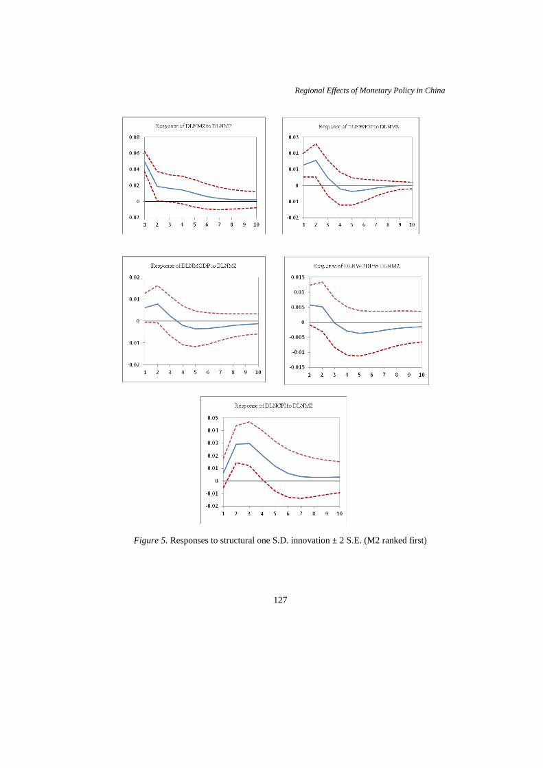
Figure 5 displays the impulse responses to a structural one-standard-deviation (4.9948%) unanticipated increase in M2 change. The growth of EGDP begins to increase at the first year and reaches a maximum 1.5688% increase at the second year. The response becomes negative after the fourth year and then gradually dies out to zero. MGDP growth has its maximum increase (0.7805%) at the second year, and the growth of WGDP has its maximum increase (0.5734%) at the first year. The price level response reaches its peak (2.9633%) at the third year and then gradually decreases to zero.

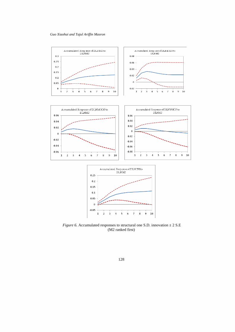
Figure 6 shows accumulated responses to a structural one S.D. (4.9948%) unanticipated increase in M2 change. We can see that the maximum cumulative increase of EGDP growth is 3.3272% at the third year. After six years, the cumulative response remains stable (2.2855%, at the 10th year). The cumulative maximum increase of MGDP growth is 1.6292% at the third year. The response then decreases gradually and asymptotes to zero at the 10th year. The maximum cumulative increase of WGDP growth is 1.0862% at the second year. The response then decreases gradually and becomes negative after six years. Finally, it remains stable at –0.7073% at the 10th year. The responses of M2 and CPI increase gradually and remain stable after six years.

Comparing the impulse responses of first SVAR model with those of the second SVAR model, we can see clearly that the results of the second model are much better. When monetary policy is allowed to influence output and inflation instantaneously, the responses of all variables are much larger. For example, in the first model, the cumulative response of MGDP growth becomes negative after six years and remains at –0.3865% at the 10th year. By comparison, when monetary policy is allowed to influence output and inflation instantaneously, the cumulative response of MGDP growth remains positive in all periods and gradually asymptotes to zero at the 10th year. Therefore, the second order of variables is better than the first order. Accordingly, we run our other SVAR analyses using the second ordering of variables: MP, EGDP, MGDP, WGDP, Price. The monetary policy variable ranks first.


127

Figure 5. Responses to structural one S.D. innovation ± 2 S.E. (M2 ranked first)


128

Figure 6. Accumulated responses to structural one S.D. innovation ± 2 S.E (M2 ranked first)


129

Impulse response to M1

Our first and second SVAR models use M2 as the monetary policy variable. Our third model will use M1 as the monetary policy variable. The order of variables is the same as in our second SVAR model: MP, EGDP, MGDP, WGDP, Price. M1 ranks first and the lag length is one. We use the same identification matrices used the first and second SVAR models. This model is also stable and the third SVAR-generated impulse response graphs are presented in Figures 7 and 8.

Figure 7 displays the impulse responses to a structural one-standard-deviation (6.6839%) unanticipated increase in M1 change. Changes in the three regions' GDP growths all exhibit the same trend: they initially increase and reach their peaks within two years. The responses become negative after the third year and gradually asymptote to zero in the long run. The growth of EGDP reaches a maximum 1.2936% increase at the first year. The MGDP growth has its maximum increase of 0.8451% at the second year and the maximum increase of WGDP growth (0.5933%) occurs at the second year. The price level response reaches its peak (3.2272%) at the second year, and then decreases gradually to zero.

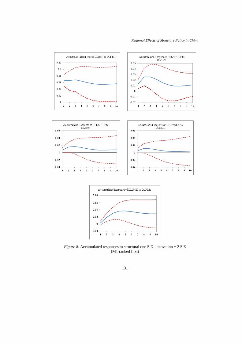
Figure 8 shows accumulated responses to the innovation (6.6839%) of M1. We can see that the cumulative responses of the three regions' respective GDP growths remain positive during the entire period. The maximum cumulative increase of EGDP growth is 2.5695% at the second year. After six years, the cumulative response remains stable (1.1325%, at the 10th year). The maximum cumulative increase of MGDP growth is 1.6716% at the third year. Then, the response gradually approaches 0.7862% at the 10th year. The maximum cumulative increase of WGDP growth is 1.1427% at the second year. Then, the response decreases gradually and remains stable (0.3983%, at the 10th year). The response of CPI increases gradually and remains stable after six years.


130

Figure 7. Responses to structural one S.D. innovation ± 2 S.E. (M1 ranked first)


131

Figure 8. Accumulated responses to structural one S.D. innovation ± 2 S.E (M1 ranked first)


132

Impulse response to one-year bank lending rate

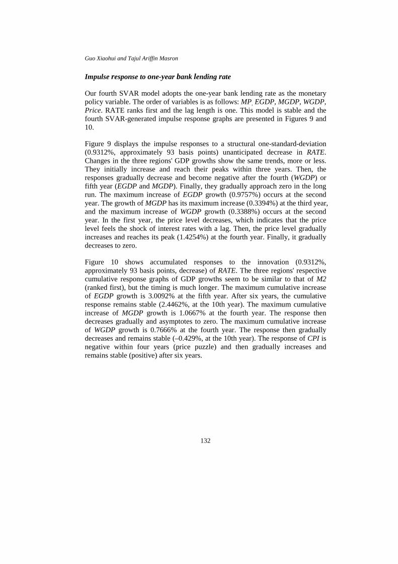
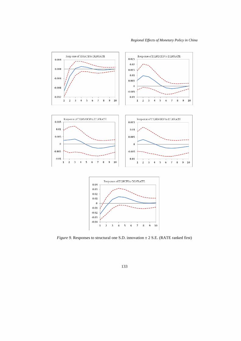
Our fourth SVAR model adopts the one-year bank lending rate as the monetary policy variable. The order of variables is as follows: MP, EGDP, MGDP, WGDP, Price. RATE ranks first and the lag length is one. This model is stable and the fourth SVAR-generated impulse response graphs are presented in Figures 9 and 10.

Figure 9 displays the impulse responses to a structural one-standard-deviation (0.9312%, approximately 93 basis points) unanticipated decrease in RATE. Changes in the three regions' GDP growths show the same trends, more or less. They initially increase and reach their peaks within three years. Then, the responses gradually decrease and become negative after the fourth (WGDP) or fifth year (EGDP and MGDP). Finally, they gradually approach zero in the long run. The maximum increase of EGDP growth (0.9757%) occurs at the second year. The growth of MGDP has its maximum increase (0.3394%) at the third year, and the maximum increase of WGDP growth (0.3388%) occurs at the second year. In the first year, the price level decreases, which indicates that the price level feels the shock of interest rates with a lag. Then, the price level gradually increases and reaches its peak (1.4254%) at the fourth year. Finally, it gradually decreases to zero.

Figure 10 shows accumulated responses to the innovation (0.9312%, approximately 93 basis points, decrease) of RATE. The three regions' respective cumulative response graphs of GDP growths seem to be similar to that of M2 (ranked first), but the timing is much longer. The maximum cumulative increase of EGDP growth is 3.0092% at the fifth year. After six years, the cumulative response remains stable (2.4462%, at the 10th year). The maximum cumulative increase of MGDP growth is 1.0667% at the fourth year. The response then decreases gradually and asymptotes to zero. The maximum cumulative increase of WGDP growth is 0.7666% at the fourth year. The response then gradually decreases and remains stable (–0.429%, at the 10th year). The response of CPI is negative within four years (price puzzle) and then gradually increases and remains stable (positive) after six years.


133

Figure 9. Responses to structural one S.D. innovation ± 2 S.E. (RATE ranked first)


134

Figure 10. Accumulated responses to structural one S.D. innovation ± 2 S.E (RATE ranked first)


135

Summary

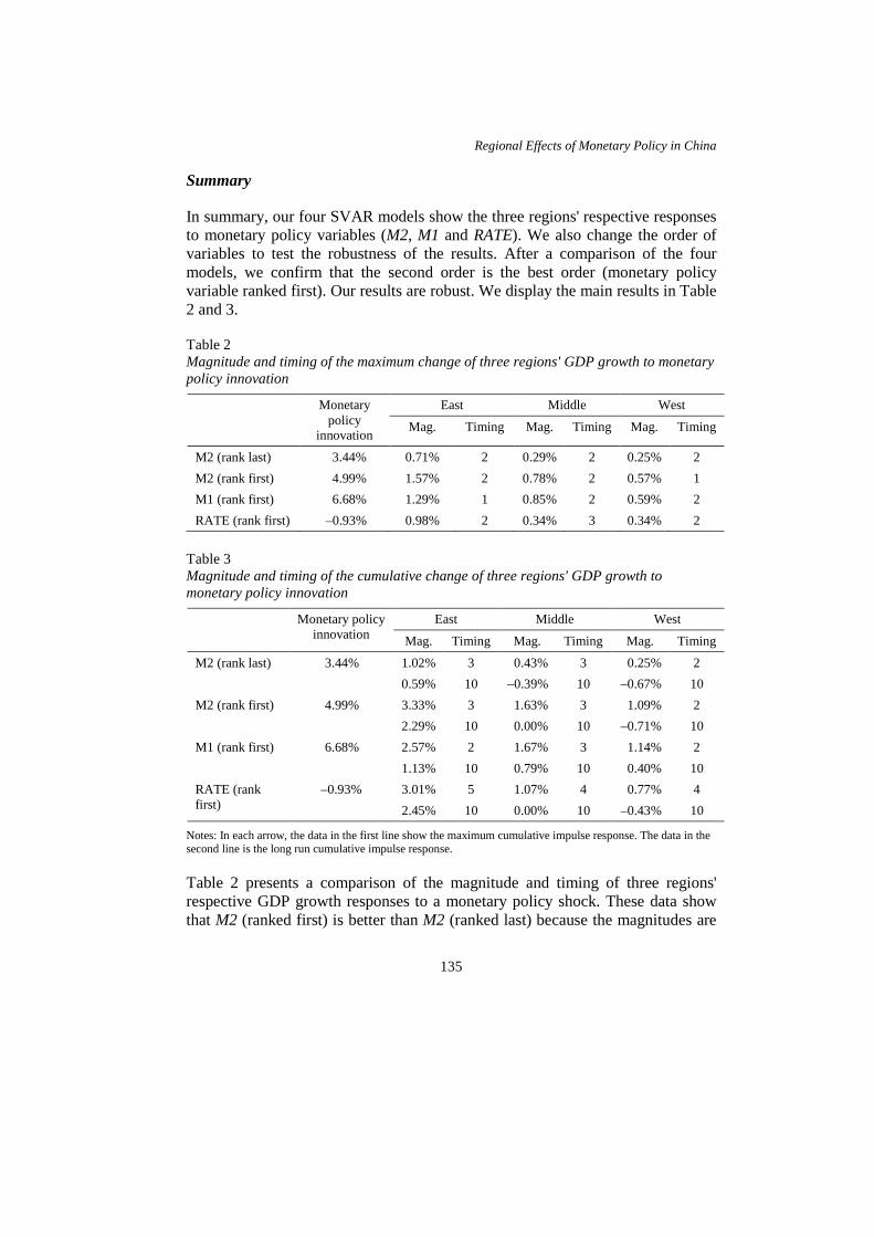
In summary, our four SVAR models show the three regions' respective responses to monetary policy variables (M2, M1 and RATE). We also change the order of variables to test the robustness of the results. After a comparison of the four models, we confirm that the second order is the best order (monetary policy variable ranked first). Our results are robust. We display the main results in Table 2 and 3.

Table 2 Magnitude and timing of the maximum change of three regions' GDP growth to monetary policy innovation

Monetary policy

innovation

East Middle West

Mag. Timing Mag. Timing Mag. Timing

M2 (rank last) 3.44% 0.71% 2 0.29% 2 0.25% 2 M2 (rank first) 4.99% 1.57% 2 0.78% 2 0.57% 1 M1 (rank first) 6.68% 1.29% 1 0.85% 2 0.59% 2 RATE (rank first) –0.93% 0.98% 2 0.34% 3 0.34% 2

Table 3 Magnitude and timing of the cumulative change of three regions' GDP growth to monetary policy innovation

Monetary policy innovation

East Middle West


M2 (rank last) 3.44% 1.02% 3 0.43% 3 0.25% 2 0.59% 10 –0.39% 10 –0.67% 10

M2 (rank first) 4.99% 3.33% 3 1.63% 3 1.09% 2 2.29% 10 0.00% 10 –0.71% 10

M1 (rank first) 6.68% 2.57% 2 1.67% 3 1.14% 2 1.13% 10 0.79% 10 0.40% 10

RATE (rank first)

–0.93% 3.01% 5 1.07% 4 0.77% 4 2.45% 10 0.00% 10 –0.43% 10

Notes: In each arrow, the data in the first line show the maximum cumulative impulse response. The data in the second line is the long run cumulative impulse response.

Table 2 presents a comparison of the magnitude and timing of three regions' respective GDP growth responses to a monetary policy shock. These data show that M2 (ranked first) is better than M2 (ranked last) because the magnitudes are


136

much bigger. An examination of the regional effects of monetary policy using annual data demonstrates the reasonableness of the assumption that monetary policy can affect output and inflation within one period. Therefore, we should rank the monetary policy variable first among all variables. According to the magnitude and timing of the three regions' responses, M2 is the best monetary policy indicator among the three indicators (M2, M1and RATE).

Table 3 shows the maximum responses and long-run responses (10 years) of the three regions. The maximum responses indicate that M2 is the best indicator among the three indicators. The long-run response levels suggest that M1 also is a good indicator because the long-run responses of all three regions remain positive with M1 ranked first. However, the long-run responses of the three regions to M2 (ranked first) and RATE are rather similar, which shows the robustness of the results. Therefore, we think that M2 is the best measure of monetary policy. Accordingly, when examining the regional effects of monetary policy, we use M2 (ranked first) as our benchmark monetary policy variable, and we use M1 and RATE as complementary analyses.

According to Tables 2 and 3 (M2 (ranked first) as our benchmark variable), when there is an unanticipated increase (4.99%) in M2 change, EGDP growth shows the biggest magnitude of increase (1.57%). This is almost twice the magnitude of the response of MGDP growth and three times the magnitude of the response of WGDP growth. Similar results are obtained for the cumulative maximum responses of the three regions' GDP growths to a M2 shock (3.33%, 1.63% and 1.09% for the East, Middle and West, respectively). With respect to long-run cumulative response levels, the cumulative response of EGDP growth is positive (3.33%), the long-run cumulative response of MGDP is about zero, and the long-run cumulative response of WGDP growth is negative (–0.71%). Hence, we can see that common monetary policy provides a significant stimulus for economic growth in the East but has less impact in the Middle and West. Moreover, the gap among the three regions keeps widening.

The Spillover Effects

The main advantage of our SVAR analysis is that we consider the spillover effects among the three regions. We argue that the influence of spillover effects should be emphasised when examining the regional effects of monetary policy, and the shortcoming of previous studies is that they ignore these effects. Because the previous studies ignoring spillover effects also use different control variables, different periods and different regional divisions, a direct comparison of our results to theirs is impossible and meaningless. Therefore, we estimate regional


137

SVAR models that do not consider spillover effects to compare to our benchmark SVAR model. This comparison highlights the importance of spillover effects.

Figure 11. Responses and accumulated responses to structural one S.D. innovation ± 2 S.E (M2)


138

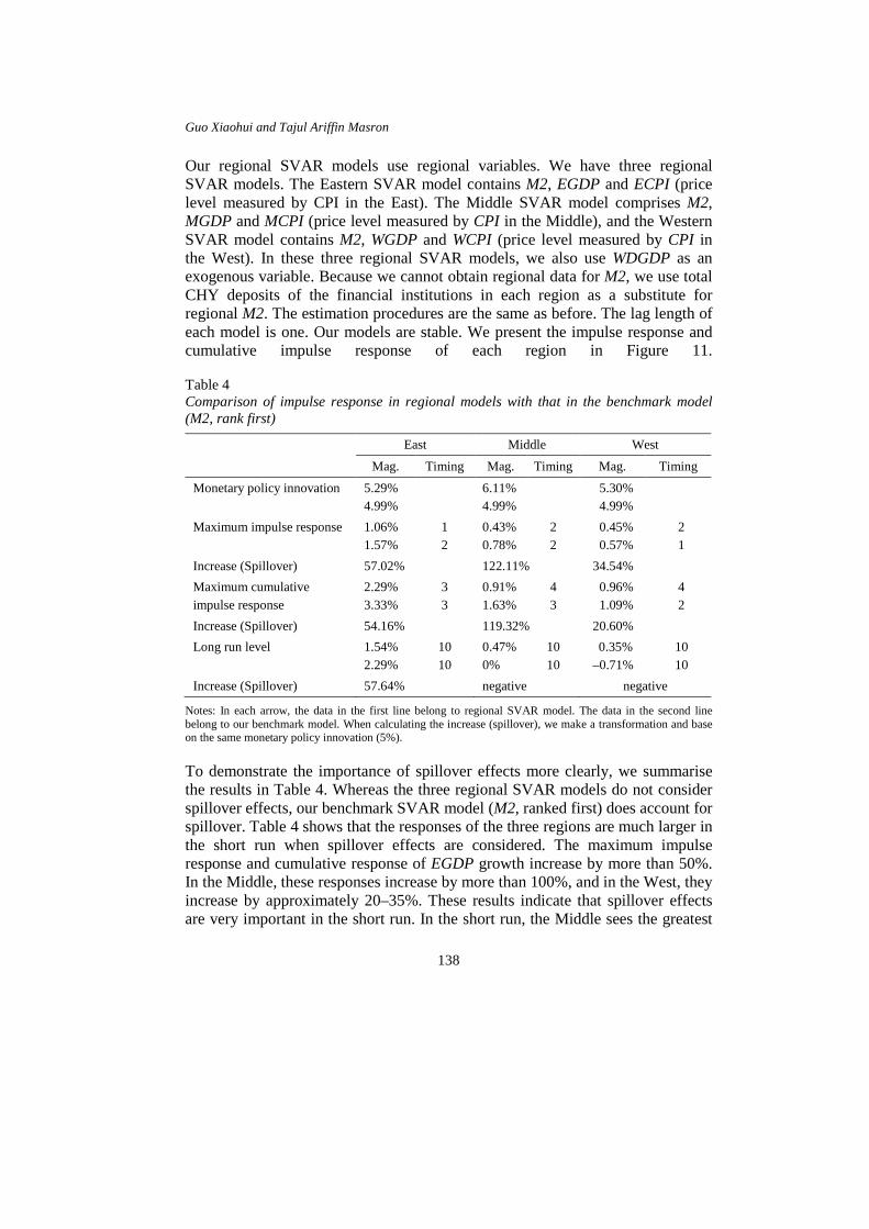
Our regional SVAR models use regional variables. We have three regional SVAR models. The Eastern SVAR model contains M2, EGDP and ECPI (price level measured by CPI in the East). The Middle SVAR model comprises M2, MGDP and MCPI (price level measured by CPI in the Middle), and the Western SVAR model contains M2, WGDP and WCPI (price level measured by CPI in the West). In these three regional SVAR models, we also use WDGDP as an exogenous variable. Because we cannot obtain regional data for M2, we use total CHY deposits of the financial institutions in each region as a substitute for regional M2. The estimation procedures are the same as before. The lag length of each model is one. Our models are stable. We present the impulse response and cumulative impulse response of each region in Figure 11. Table 4 Comparison of impulse response in regional models with that in the benchmark model (M2, rank first)

East Middle West


Monetary policy innovation 5.29% 4.99%

6.11% 4.99%

5.30% 4.99%

Maximum impulse response 1.06% 1.57%

1 2

0.43% 0.78%

2 2

0.45% 0.57%

2 1

Increase (Spillover) 57.02% 122.11% 34.54% Maximum cumulative impulse response

2.29% 3.33%

3 3

0.91% 1.63%

4 3

0.96% 1.09%

4 2

Increase (Spillover) 54.16% 119.32% 20.60% Long run level 1.54%

2.29% 10 10

0.47% 0%

10 10

0.35% –0.71%

10 10

Increase (Spillover) 57.64% negative negative

Notes: In each arrow, the data in the first line belong to regional SVAR model. The data in the second line belong to our benchmark model. When calculating the increase (spillover), we make a transformation and base on the same monetary policy innovation (5%).

To demonstrate the importance of spillover effects more clearly, we summarise the results in Table 4. Whereas the three regional SVAR models do not consider spillover effects, our benchmark SVAR model (M2, ranked first) does account for spillover. Table 4 shows that the responses of the three regions are much larger in the short run when spillover effects are considered. The maximum impulse response and cumulative response of EGDP growth increase by more than 50%. In the Middle, these responses increase by more than 100%, and in the West, they increase by approximately 20–35%. These results indicate that spillover effects are very important in the short run. In the short run, the Middle sees the greatest


139

amount of spillover effects, followed by the East. The West sees the smallest level of spillover. In the long run, the three regions' respective responses are all positive when spillover effects are ignored. By contrast, when spillover effects are considered, only the long-run response of EGDP growth increases by more than 50%, whereas the long-run responses of the Middle and West are both negative.

The reason for the differences between the short- and long-run results is the transfer of bank deposits from one region to another in China. Specifically, the banking system in China is monopolised by four state-owned joint-stock banks (the Industrial and Commercial bank of China, the Bank of China, the Construction Bank of China and the Agricultural Bank of China). These four banks have adopted branch-banking systems, and their respective branches are located throughout the country. In the past thirty years, branches in the Middle and West have collected a substantial sum of deposits. However, not all of these deposits are used to support the development of the Middle and West. Because the East has developed much faster, some of the deposits collected in the Middle and West are transferred to branches in the East to support the development of that region.

In our SVAR model, we use M2 as monetary policy variable. In the short run, spillover effects work because the deposits have no time to transfer. Therefore, in the short run, the spillover effects are very significant. However, deposits have plenty time to transfer in the long run. The negative influence of fund transfers is much larger than the positive influence of spillover effects. Accordingly, when spillover effects are considered, the long-run levels of cumulative responses of MGDP growth and WGDP growth are zero and negative, respectively. However, if we assume that all growth deposits collected in a particular region are used for the development of that region (our regional models), the long-run level of cumulative responses of MGDP growth and WGDP growth are both positive. This means that the rapid growth of the East over the past thirty years has been at the expense of growth in the Middle and West (the long-run cumulative response of EGDP growth shows an increase of more than 50% when spillover effects are considered, whereas the long-run cumulative responses of MGDP growth and WGDP growth are both negative). This phenomenon also indicates that previous analyses of the regional effects of monetary policy in China that do not account for spillover effects tend to overestimate the long-run responses of the Middle and West and underestimate the long-run effects in the East.


140

This explanation also can be proved by the data presented in Figure 8. M1 comprises primarily cash and demand deposits. It is highly liquid and impossible to transfer across regions. Therefore, the long-run cumulative responses of MGDP growth and EGDP growth are both positive.

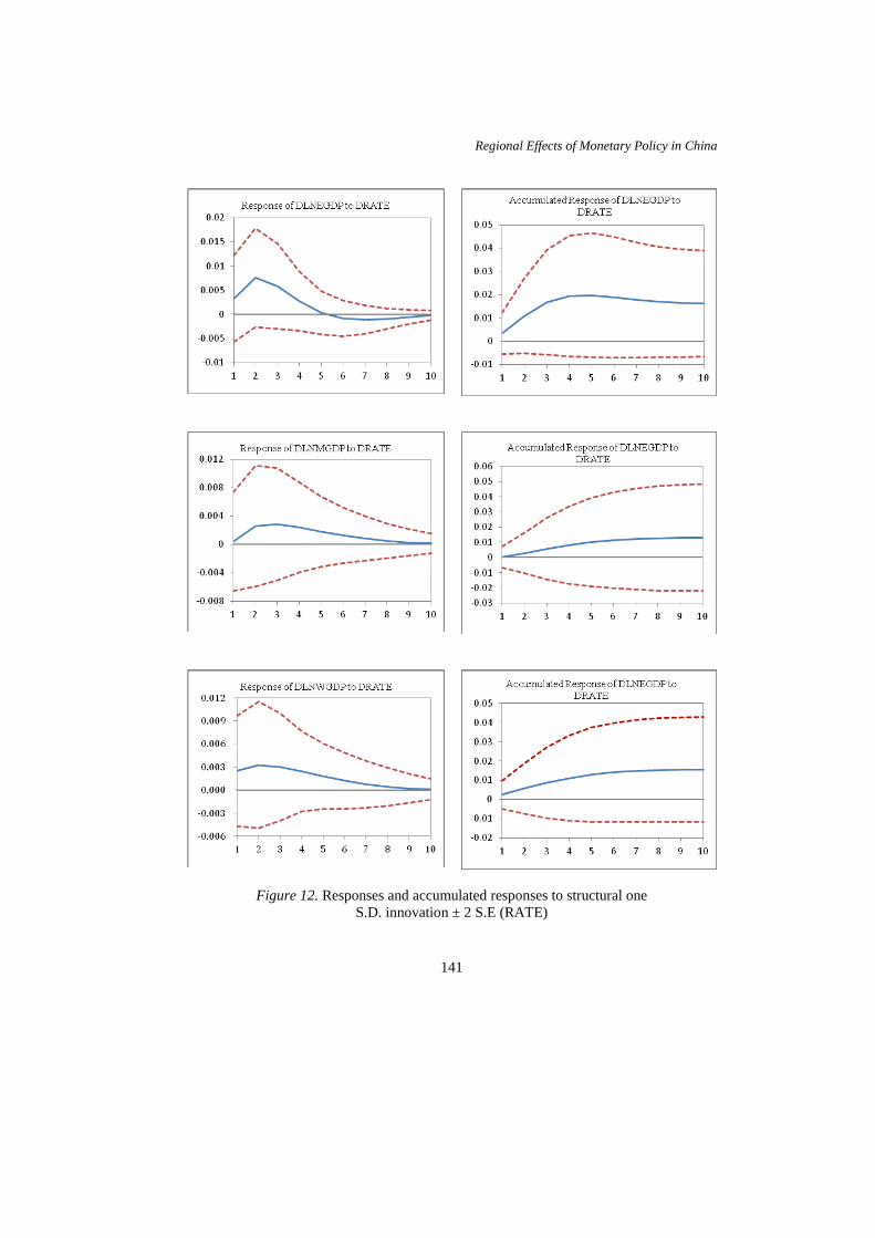
Some may question the use of total CHY deposits in a region's financial institutions to measure M2 in our regional models. This measurement may account to some extent for spillover effects. However, to show the robustness of our results, we also use the one-year bank lending rate as the monetary policy variable in our three regional SVAR models. The results are shown in Figure 12 and Table 5. Table 5 demonstrates that spillover effects remain very important and our results are rather robust.

Table 5 Comparison of impulse response in regional models with that in our national model (RATE)

East Middle West


Monetary policy innovation –0.93% –0.93%

–0.97% –0.93%

–0.96% –0.93%

Maximum impulse response 0.76% 0.98%

2 2

0.28% 0.34%

3 3

0.32% 0.34%

2 2

Increase (Spillover) 28.95% 26.65% 9.68% Maximum cumulative impulse response

1.98% 3.01%

5 5

– 1.07%

– 4

– 0.77%

– 4

Increase (Spillover) 52.02% – – Long run level 1.61%

2.45% 10 10

1.31% 0%

10 10

1.56% –0.43%

10 10

Increase (Spillover) 52.17% negative negative

Notes: In each arrow, the data in the first line belong to regional SVAR model. The data in the second line belong to our national model. When calculating the increase (spillover), we make a transformation and base on the same monetary policy innovation (–1%).


141

Figure 12. Responses and accumulated responses to structural one S.D. innovation ± 2 S.E (RATE)


142

CONCLUSION

This paper uses annual data from 1978 to 2011 for the three regions of China to study the regional effects of common monetary policy. We propose a SVAR model that includes real and monetary variables to identify output responses to monetary policy. The results confirm that the three regions respond differently to monetary policy. The East shows the largest response, the Middle shows the second-largest response, and the West shows the smallest response. These findings confirm that in China, common monetary policy has different impacts on different regional economies. Moreover, the different regional effects of monetary policy widen the economic gap among the three regions.

When the PBC formulates and implements common monetary policy, it should take these different effects into account. In fact, the PBC has already implemented the Differentiated Deposit Requirement Ratio (DDRR)4 policy, whose primary purpose was to restrain lending by financial institutions with inadequate capital and poor asset quality. However, the PBC recently expanded the use of this policy to support certain less-developed rural regions. For example, they applied a lower DDRR to support the reconstruction of the earthquake-stricken area (six cities in Sichuan province) from 2008:06 to 2011:06. If we can prove that this use of DDRR policy supports the economic growth of this disaster area (another paper, forthcoming), then we can suggest that the PBC consider expanding this application of DDRR policy to less-developed regions (the Middle and West) or rural areas to promote more coordinated regional economic development.

We also check the results using different monetary policy variables: M2, M1 and the one-year bank lending rate. The results show that M2 is the best monetary policy indicator among these variables because M2 provides satisfactory and robust results.

We also examine the importance of spillover effects. We compare the results of our benchmark SVAR model with the regional SVAR models and find that in the short run, spillover effects are very important. However, in the long run, the influence of deposit transfers is much larger than the impact of spillover effects. Therefore, in the past thirty years, the rapid growth of the East has been at the expense of growth in the Middle and West. We also find that previous studies that examine the regional effects of monetary policy without accounting for spillover effects tend to underestimate the influence of monetary policy on each region in the short run. In addition, in the long run, they overestimate the influence of monetary policy in the Middle and West and underestimate its effects in the East.


143

This study also has several limitations. First, because of the lack of quarterly regional GDP data, we must use annual data. Thirty-four years of data, from 1978 to 2011, may be not enough. Moreover, China has undergone substantial economic changes in the past three decades. Due to the data limitations, we cannot check the structural break by dividing the estimation period.

Second, in the past 30 years, the monetary policy instruments used by the PBC have changed several times. Currently, the PBC uses a variety of monetary policy instruments simultaneously to regulate the economy. Some authors, such as Sun (2013), indicate that one single instrument might not adequately represent the monetary policy stance. He, Leung and Chong (2013) also suggest that an analysis based on a single monetary tool may not provide a good evaluation of the PBC's monetary policy. Xiong (2012) summarises information regarding several monetary policy instruments and develops a new policy stance index. He et al. (2013) suggest a factor that tracks a wide range of the market-based policy instruments that are at the disposal of the PBC to represent the general stance of the monetary policy. Unfortunately, the empirical periods covered by these studies are limited to recent years (after 1998). Because our estimation period covers the initiation of economic reform and opening up in 1978 until 2011, we cannot obtain such a policy stance index due to the data limitations. These shortcomings may be resolved when the information and data problems are addressed. NOTES 1. According to the Western Development Strategy enacted in 2000, the eastern region

contains 11 provinces: Beijing, Tianjin, Hebei, Liaoning, Shanghai, Jiangsu, Zhejiang, Fujian, Shandong, Guangdong and Hainan. The middle region comprises 8 provinces: Shanxi, Jilin, Heilongjiang, Anhui, Jiangxi, Henan, Hubei and Hunan. The western region is made up of 12 provinces: Neimenggu, Guangxi, Chongqing, Sichuan, Guizhou, Yunnan, Tibet, Shaanxi, Gansu, Qinghai, Ningxia and Xinjiang. The term "coastal areas" refers to the eastern region and the term "inland areas" refers to the middle and western regions.

2. When monetary policy shocks are identified with innovations in interest rates, the responses of output and money supply are correct because monetary tightening (an increase in interest rates) is associated with a decrease in money supply and output. However, the response of the price level is incorrect because monetary tightening is associated with an increase in the price level, not a decrease (see Sims, 1992).

3. The Taylor (1993) rule proposes that central banks should modify nominal interest rates based on gaps between the target inflation rate and the expected inflation rate and between target output and expected output. The McCallum (1988) rule describes


144

how money supply can be used as a tool to achieve target outputs and inflation rates and is a parallel to the Taylor rule. The two rules describe how central banks raise (reduce) interest rates (money supply) when the expected inflation is higher (lower) than the target inflation rate and when actual output is greater (smaller) than natural output.

4. The essence of DDRR policy is that the required reserve ratio applicable to a financial institution is based on indicators such as its capital-adequacy ratio and asset quality. The lower the capital-adequacy ratio of a financial institution and the higher its NPL (Non-Performing Loan) ratio, the higher the applicable required reserve ratio.

REFERENCES

Beare, J. B. (1976). A monetarist model of regional business cycles. Journal of Regional Science, 16(1), 57.

Bernanke, B. S., & Blinder, A. S. (1992). The federal funds rate and the channels of monetary transmission. American Economic Review, 82(4), 901–921.

Brun, J. F., Combes, J. L., & Renard, M. F. (2002). Are there spillover effects between coastal and non-coastal regions in China? China Economic Review, 13(2–3), 161–169.

Carlino, G., & DeFina, R. (1996). Does monetary policy have differential regional effects? Federal Reserve Bank of Philadelphia Business Review (March/April 1996), 17–27.

Carlino, G., & DeFina, R. (1998). The differential regional effects of monetary policy. Review of Economics & Statistics, 80(4), 572–587.

Carlino, G., & DeFina, R. (1999). The differential regional effects of monetary policy: Evidence from the U.S. states. Federal Reserve Bank of Philadelphia Business Review Working Paper, No. 97-12/R, 1–30.

Chen, M., & Zheng, Y. (2008). China's regional disparity and its policy responses. China & World Economy, 16(4), 16–32.

Cohen, J., & Maeshiro, A. (1977). The significance of money on the state level: Note. Journal of Money, Credit and Banking, 9(4), 672–678.

Cortes, B. S., & Kong, D. (2007). Regional effects of Chinese monetary policy. The International Journal of Economic Policy Studies 2, 15–28.

De Lucio, J. J., & Izquierdo, M. (1999). Local responses to a global monetary policy - The regional structure of financial system. Fundación de Estudios de Economía Aplicada, FEDEA – D.T. 99-14, 1–24.

Di Giacinto, V. (2003). Differential regional effects of monetary policy: A geographical SVAR approach. International Regional Science Review, 26(3), 313–341.

Dickinson, D., & Liu, J. (2007). The real effects of monetary policy in China: An empirical analysis. China Economic Review, 18(1), 87–111.

Fan, L., Yu, Y., & Zhang, C. (2011). An empirical evaluation of China's monetary policies. Journal of Macroeconomics, 33(2), 358–371.

Fan, S., Kanbur, R., & Zhang, X. (2011). China's regional disparities: Experience and policy. Review of Development Finance, 1(1), 47–56.


145

Fishkind, H. H. (1977). The regional impact of monetary policy: An economic simulation study of Indiana 1958–1973. Journal of Regional Science, 17(1), 77.

Fleisher, B., Haizheng, L., & Minqiang, Z. (2008). Human capital, economic growth, and regional inequality in China. RPRT. IZA Discussion Papers, Institute for the Study of Labor (IZA).

Garrison, C. B., & Chang, H. S. (1979). The effect of monetary and fiscal policies on regional business cycles. International Regional Science Review, 4(2), 167–180.

Garrison, C. B., & Kort, J. R. (1983). Regional impact of monetary and fiscal policy: A comment. Journal of Regional Science, 23(2), 249–261.

Georgopoulos, G. (2009). Measuring regional effects of monetary policy in Canada. Applied Economics, 41(16), 2093–2113.

Groenewold, N., Lee, G., & Chen, A. (2007). Regional output spillovers in China: Estimates from a VAR model. Papers in Regional Science, 86(1), 101–122.

He, Q., Leung, P. H., & Chong, T. T. L. (2013). Factor-augmented VAR analysis of the monetary policy in China. China Economic Review, 25, 88–104.

Hsing, Y., & Hsieh, W. (2004). Impacts of monetary, fiscal and exchange rate policies on output in China: A VAR approach. Economics of Planning, 37(2), 125–139.

Jeon, Y., & Miller, S. M. (2004). The geographic distribution of the size and timing of monetary policy actions (Working Paper 2004–22). Department of Economics, University of Connecticut, pp. 1–37.

Jiang, Y., & Chen, Z. (2009) (in Chinese). Empirical analysis of regional effects of monetary policy employing SVAR in China. Journal of Financial Research, 346(4), 180–195.

Kanbur, R., & Zhang, X. (2005). Fifty years of regional inequality in China: A journey through central planning, reform, and review of development economics. Review of Development Economics, 9(1), 87–106.

Kong, D., Cortes, B. S., & Qin, D. (2007) (in Chinese). Empirical analysis of provincial effectiveness of monetary policy in China. Journal of Financial Research, 330(12), 17–26.

Lau, C. K. M. (2010). New evidence about regional income divergence in China. China Economic Review, 21(2), 293–309.

Mathur, V. K., & Stein, S. (1983). Regional impact of monetary and fiscal policy: A comments. Journal of Regional Science, 23(2), 249.

McCallum, B. (1998). Robustness Properties of a rule for monetary policy. Carnagie-Rochester Conference Series on Public Policy, 29, 173–203.

Mundell, R. A. (1961). A theory of optimum currency areas. The American Economic Review, 51(4), 657–665.

Nachane, D. M., Ray, P., & Ghosh, S. (2002). Does monetary policy have differential state-level effects? An empirical evaluation. Economic and Political Weekly, 37(47), 4723–4728.

Owyang, M. T., & Wall, H. J. (2005). Structural breaks and regional disparities in the transmission of monetary policy (Working Paper Series 2003–008C), Federal Reserve Bank of St. Louis, pp. 1–36.

Pedroni, P., & Yao, J. Y. (2006). Regional income divergence in China. Journal of Asian Economics, 17(2), 294–315.


146

Sims, C. A. (1992). Interpreting the macroeconomic time series facts: The effects of monetary policy. European Economic Review, 36(5), 975–1000.

Sims, C. A., & Zha, T. A. (1995). Does monetary policy generate recessions. Working Paper, Yale University.

Song, W., & Zhong, Z. (2006) (in Chinese). The existence and origin of regional effects of monetary policy in China–An analysis based on the theory of optimum currency areas. Economic Research Journal, 3, 46–58.

Sun, R. (2013). Does monetary policy matter in China? A narrative approach. China Economic Review, 26, 56–74.

Taylor, J. B. (1993). Discretion versus policy rules in practice. Carnagie-Rochester Conference Series Public Policy, 39, 195–214.

Weber, E. J. (2006). Monetary policy in a heterogeneous monetary union: The Australian Experience. Applied Economics, 38(21), 2487–2495.

Xiong, W. (2012). Measuring the monetary policy stance of the People’s Bank of China: An ordered probit analysis. China Economic Review, 23(3), 512–533.

Ying, L. G. (2000). Measuring the spillover effects: Some Chinese evidence. Papers in Regional Science, 79(1), 75–89.

Zhang, X., & Zhang, K. H. (2003). How does globalization affect regional inequality within a developing country? Evidence from China. The Journal of Development Studies, 39(4), 47–67.

Documents

REGIONAL EFFECTS OF MONETARY POLICY IN …web.usm.my/aamj/19012014/Art 6 (113-146).pdf · The Literature in Other Countries When discussing the regional effects of monetary policy,