Embed Size (px)
Citation preview
Preliminary Draft Do not quote
Regional Differences in the Labor Market Impact of Immigration: Evidence from Spain
Catalina Amuedo-Dorantes Department of Economics
San Diego State University & IZA e-mail: [email protected]
Sara de la Rica Depto. Fundamentos del Análisis Económico II
Universidad del País Vasco & IZA e-mail: [email protected]
I. Introduction
How immigration affects the labor market of the host country is a topic of major
concern for many immigrant-receiving nations. Spain is no exception following the
rapid increase in immigrant flows experienced over the past decade. In 1991, only 1.2
percent of the Spanish adult population (about 300,000 individuals) was foreign-born.
Within a decade, this percentage quadrupled to 4.0 percent (1,370,000 individuals) and,
by 2005, it reached 8.0 percent (3,100,000 individuals). Not surprisingly, about 60
percent of Spanish citizens declared immigration as their main social concern, before
unemployment, housing and terrorism (CIS, September 2006). Yet, immigration
concerns vary by region along with the geographic distribution and impact of
immigrants. Indeed, most immigrants are concentrated in a few Spanish regions that
absorb about 83.5 percent of the immigrant flow and where immigrants represent up to
17 percent of the adult working population, i.e. Andalucía, Balearic Islands, Canary
Islands, Cataluña, Valencia, Madrid and Murcia (see Tables 1 and 2).
How has immigration affected Spanish natives? And, does this impact differ
substantially by region? In this paper, we address these two questions with an analysis
of the impact of recent immigration flows to the Spanish economy while taking into
account regional differences. As in the Hecksher-Olin Model, where trade raises
national income if the factor shares in the trading partner differ from those in the home
country, immigration raises income inasmuch the skill shares of the inflow of
immigrants differ from those of natives. The greater the difference between the skill
shares of natives and immigrants, the greater the increase in income will be. This
implies that the increase in income depends on the degree of substitutability between
natives and immigrants, with an underlying redistribution of income from groups of
natives to those of incoming immigrants with similar skills as well as to groups of
1

immigrants and natives with complementary skills. It is this income redistribution that
often lies behind anti-immigration sentiments and, more importantly, substantiates the
need to gain a better understanding of the consequences that immigrant concentration
may have on the well-being of natives at the regional and national levels.
To date, most studies concerning the effects of immigration on natives on
account of the differential skill share between immigrant and native groups have
focused on the impact of immigration on the national economy (e.g. Altonji and Card
2001; Card 2001; Borjas 1995, 2003; Ottaviano and Peri 2005, 2006). Peri (2006) is an
exception with its focus on the effect of immigration on natives’ wages in California.
The present study follows this literature and computes the net immigration surplus (IS)
accruing to the various Spanish regions on account of the uneven distribution of
immigrants throughout Spain and the regional variation in skills between immigrants
and natives. At the core of these figures lays a crucial policy question regarding the role
of immigration in balancing out differences in the supply of specific skills across
regions and, in that manner, in reducing regional labor market disequilibria.
The rest of the paper is organized as follows: Section II provides a description of
the data we will be using in our analysis and Section III discusses some descriptive
evidence on the regional distribution by skill level of the foreign-born relative to
natives. Section IV presents the production function we use in our structural approach
to estimate the IS in each of the main immigrant-receiving regions as well as at the
national level. Results and shortcomings of the analysis are discussed in Sections V and
VI, respectively, whereas Section VII concludes the study.
II. Data
In our analysis, we use the 2001 Census data. The Census has the advantage of,
in principle, interviewing all immigrants regardless of their legal status. Nonetheless,
2

we are aware that an important fraction of unauthorized immigrants may not fill in the
questionnaire and, as such, this group is likely to be under-represented in the Census.
The Census gathers information on personal and demographic characteristics (such as
age, education or province of residence). This information is used to group individuals
into education and experience (proxied using age and educational attainment) cells.
However, the Census is limited with respect to the list of variables for which
data are compiled. For instance, it lacks information on where respondents completed
their schooling; as such, we are left to assume that, for our group of recent migrants, this
is likely to have taken place in their countries of origin.1 Additionally, the Census does
not contain any data on language skills or on the nationality of respondents’ parents and
grandparents. As such, we define immigrants as individuals reporting a foreign
nationality. More important to the study at hand is the lack of information on labor
earnings in the Census. To supplement this shortcoming, we rely on wage data from the
1995 and 2002 Earnings Structure Surveys –known by their acronyms of EES-95 and
EES-02. These surveys include random samples of establishments in the
manufacturing, construction and service industries. Additionally, we make use of the
1995 and 2002 Current Population Surveys, which contain detailed information on
employment and immigration for those two years –data we rely upon to compute
employment and wages for natives and immigrants in various skill groups later on.
III. Some Descriptive Evidence
A) Differences in the Regional Distribution of Immigrants and Natives
The figures in Table 1 and Table 2 provide testimony of the fast growing
presence of immigrants in the various Spanish regions. Specifically, the first three
columns of Table 1 display the increasing fraction of the overall adult population – 1 The Census question regarding the educational attainment of individuals 10 years of age and older is phrased as follows: “What is the highest grade you have completed?”
3

defined as individuals 16 years of age and older– with a foreign nationality. In certain
immigrant-receiving regions, such as Cataluña or Madrid, the percentage of immigrants
has grown from 2 percent to around 12 percent in approximately 14 years. As a fraction
of the adult working population, the increase is even more pronounced, moving from 2
percent to as much as 17 percent in Madrid or 19 percent in Balearic Islands.
Furthermore, as noted in the Introduction, immigrants are unevenly distributed
throughout Spain. The figures in Table 2 show that a few regions, such as Andalucía,
Balearic Islands, Canary Islands, Cataluña, Valencia, Madrid and Murcia, concentrate
most immigrants. In 1991, these Spanish regions accounted for 78 percent of all
immigrants –a percentage that grew to 83 percent by 2001. In contrast, only 65 percent
of natives lived in those regions during that period of time.
B) Differences in the Educational and Age Distribution of Immigrants and
Natives
The growingly uneven regional distribution of immigrants is, nonetheless,
accompanied by small differences in the skill shares of immigrants and natives, both at
the national and regional levels. Figures 1 through 12 display the percentage of foreign-
born and native workers with a particular educational attainment and in a specific age
group –both variables to be used in constructing education and experience groups.
Perhaps the most surprising finding from Figures 1 through 6 is the astonishing
similarity education-wise of employed immigrants and natives in Spain. Immigrants
seem to have a slight greater presence relative to natives among workers with less than a
primary education at the national level (Figure 1) and at the regional level (Figures 2
through 6). Additionally, there are some differences in the relative incidence of
immigrants among groups of workers with a secondary or university education in some
of the regions being examined but nevertheless, differences are small. For instance, the
4

fraction of immigrants with a secondary education is practically 10 percentage points
lower than the corresponding share of natives in Cataluña and Murcia. Likewise, the
share of working immigrants with a university degree is about 10 percentage points
lower than the corresponding share of working natives in Madrid and Murcia.
How distinct are the age distributions of working immigrants and natives?
Figures 7 through 12 address this question. Not surprisingly, immigrants are, overall,
younger than natives and, as such, the fraction of working immigrants of a younger age
is higher than the corresponding fraction of working natives nationwide (Figure 7).
Differences in the age distribution of both groups are particularly acute in Cataluña,
Madrid, Murcia, and Valencia (see Figures 9 through 12). For instance, the fraction of
working immigrants 25 to 34 years of age is about 10 percentage points higher than the
corresponding fraction of natives in all those regions. In contrast, the fraction of
employed immigrants 45 years of age and older in those four regions is anywhere
between 13 and 20 percentage points lower than the corresponding fraction of natives.
In sum, working immigrants and natives appear to have similar educational
attainment, even if they differ with respect to age. This apparent similarity in the
distribution of immigrants and natives education-wise can play an important role in
shaping the IS, which is proportional to the difference in skill shares between
immigrants and natives.
IV. Theoretical Framework
Our main objective is to learn about the gains to native Spaniards from
increasing immigrant flows during the past decades. Do natives benefit from
immigration? How large are those benefits? And, do these gains from immigration
fluctuate by region as a by-product of varying production complementarities between
immigrants and natives in each of those regions?
5
A) Computing the Immigration Surplus
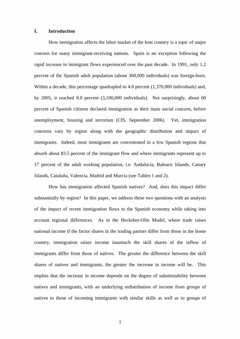
In order to address the aforementioned questions, we make use of simple
framework proposed by Borjas (1995, p.21) to estimate the immigration surplus (IS)
that accrues to natives. We adapt Borjas’ (1995) calculation of the immigrant surplus
under the assumption of homogeneous labor to a case of heterogeneous labor where
workers can present up to n different skills. We assume a production technology that
can be described by the following concave and linear homogeneous production
function:
( )1, , ..., nQ f K L L= (1)
where and ib iβ denote the shares of natives and immigrants, respectively, with a
particular skill level i, with . Each skill level i is defined in terms of educational
attainment
1...i = n
( )k and experience ( )j . Educational attainment is measured in eight
categories: less than primary, primary, secondary, first level of vocational training,
second level of vocational training, high-school, first level of a university education and
second level of a university education. Experience, on the other hand, is proxied with
age. We distinguish seven age categories: less than 30, 30-34, 35-39, 40-44, 45-49, 50-
54 and 55-65.
We make several assumptions about the production function. First, we assume
that all capital is owned by natives. Immigrants do not contribute any capital. If they
did, the IS accruing to natives would only be smaller as we shall discuss later on.
Second, the supply of labor is perfectly inelastic. As noted by Borjas (1995), this
assumption only makes the calculation of the IS simpler. Third, we assume that native
and immigrant workers within a particular skill i are perfect substitutes –an assumption
we will double check later. Fourth, we assume that capital is infinitely elastically
supplied at a constant rate r. This assumption is more realistic than assuming a fixed-
6
capital stock and it implies that all output will be distributed to workers as r. Capital
owners do not obtain any gain as there is no change in the interest rate, r. Finally, we
assume that the production function exhibits constant returns to scale. Therefore, the
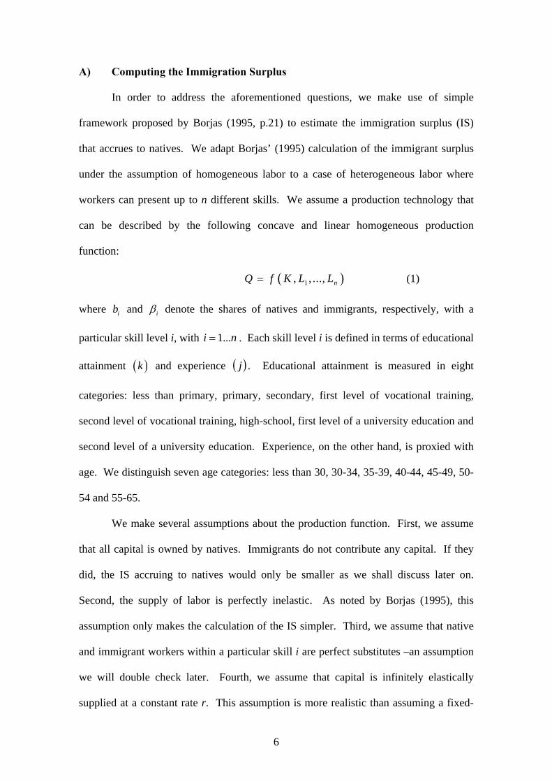
entire output is distributed among workers as r is constant. At equilibrium, the price of
each of the factors of production has to equal its corresponding value of marginal
product and the increase in income accruing to natives following the entry of M
immigrants (i.e. the increase in national income per unit of output accruing to natives) is
given by:
1 21 2( ... )N n
nQ r w w wIS K b N b N b NQ M M M M
MQ
Δ ∂ ∂ ∂ ∂= = + + + +
∂ ∂ ∂ ∂ (2)
Under the assumption that capital is infinitely elastically supplied at a constant rate r,
we can rewrite equation (2) as:
( ) ( ) ( )1 21 1 1 2 2 2
1 ...2
N nn N N
Q w wIS b N b M b N b M b N b MQ M M
β β βΔ ∂ ∂⎡ ⎤= = − + − + + −⎢ ⎥∂ ∂⎣ ⎦wM∂∂
(3)
As in free trade, immigrants create a surplus as long as their skills differ from those of
natives, i.e. the IS is positive only when ( ) 0i ib β− ≠ . Otherwise, owing to the CES
assumption, the prices of the various factors of production would remain unchanged (as
their relative supplies would remain unaltered) and natives would not gain anything
from immigration.
Given that: ( )i i ii i
i i
w w L wb i
M L M Lβ∂ ∂ ∂ ∂
= = −∂ ∂ ∂ ∂
, we can convert equation (3) into
percentage terms and measure the surplus at the average value of M, which yields the
following expression for the IS at the national level:
2
1 1
( )1 (1 )2
n nN i i
iji ji
Q b isIS m mQ p
β= =
Δ −= = − − e∑ ∑
(4)
7
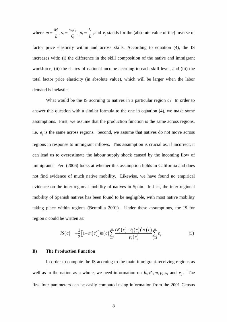
where , , ,i i ii i
w L LMm s pL Q L
= = = ijeand stands for the (absolute value of the) inverse of
factor price elasticity within and across skills. According to equation (4), the IS
increases with: (i) the difference in the skill composition of the native and immigrant
workforce, (ii) the shares of national income accruing to each skill level, and (iii) the
total factor price elasticity (in absolute value), which will be larger when the labor
demand is inelastic.
What would be the IS accruing to natives in a particular region c? In order to
answer this question with a similar formula to the one in equation (4), we make some
assumptions. First, we assume that the production function is the same across regions,
i.e. is the same across regions. Second, we assume that natives do not move across
regions in response to immigrant inflows. This assumption is crucial as, if incorrect, it
can lead us to overestimate the labour supply shock caused by the incoming flow of
immigrants. Peri (2006) looks at whether this assumption holds in California and does
not find evidence of much native mobility. Likewise, we have found no empirical
evidence on the inter-regional mobility of natives in Spain. In fact, the inter-regional
mobility of Spanish natives has been found to be negligible, with most native mobility
taking place within regions (Bentolila 2001). Under these assumptions, the IS for
region c could be written as:
ije
( ) ( ) ( ) ( ) ( ) ( )( )
2
1 1
( )1 12
n ni i i
iji ji
c b c s cIS c m c m c e
p cβ
= =
−= − −⎡ ⎤⎣ ⎦ ∑ ∑ (5)
B) The Production Function
In order to compute the IS accruing to the main immigrant-receiving regions as
well as to the nation as a whole, we need information on , , , ,i i i ib m p sβ and . The
first four parameters can be easily computed using information from the 2001 Census
ije
8
data. However, in order to compute the factor price elasticities ( )ije , we need to make
some specific assumptions regarding the technology at hand. Following Borjas (2003),
we assume a three-level CES technology. This type of production function imposes
certain simplifications. Specifically, we assume that natives and immigrants within the
same education-age group are perfect substitutes, with the elasticity of substitution
between workers with the same education (or with the same experience) being the same
across adjacent educational (or experience) categories. Therefore, under the three-level
CES production function, we assume that workers with similar educational attainment
are aggregated to form the labor supply of a particular education group. Workers of
different educational levels but with the same work experience, as captured by age, are,
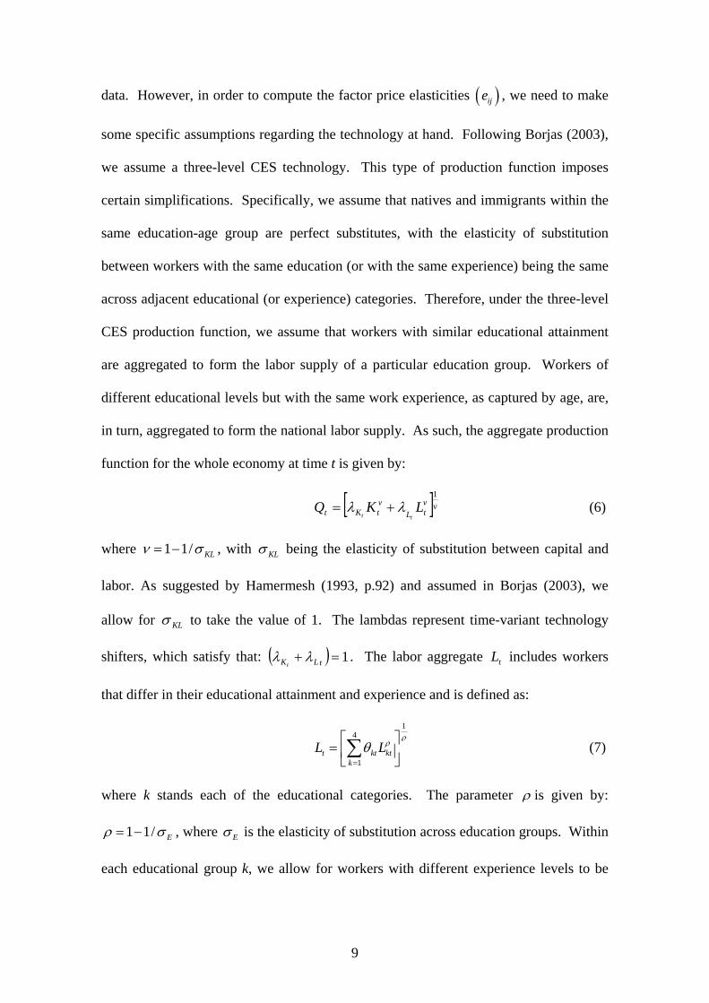
in turn, aggregated to form the national labor supply. As such, the aggregate production
function for the whole economy at time t is given by:
[ ]vvtL
vtKt LKQ
tt
1
λλ += (6)
where 1 1/ KLν σ= − , with KLσ being the elasticity of substitution between capital and
labor. As suggested by Hamermesh (1993, p.92) and assumed in Borjas (2003), we
allow for KLσ to take the value of 1. The lambdas represent time-variant technology
shifters, which satisfy that: ( ) 1=+ tLKtλλ . The labor aggregate includes workers
that differ in their educational attainment and experience and is defined as:
tL
14
1t kt k
kL L t
ρρθ
=
⎡ ⎤= ⎢ ⎥⎣ ⎦∑ (7)
where k stands each of the educational categories. The parameter ρ is given by:
1 1/ Eρ σ= − , where Eσ is the elasticity of substitution across education groups. Within
each educational group k, we allow for workers with different experience levels to be
9

imperfect substitutes. As such, the labor supply of workers within a particular
educational group at a point in time is given by:
14
1kt kj kjt
j
L Lη
ηα=
⎡ ⎤= ⎢ ⎥⎣ ⎦∑ (8)
where j are age intervals. The parameter η is given by: 1 1/ jη σ= − , where jσ
measures the elasticity of substitution between workers with different experience levels
but within the same educational group.
One advantage of the three-level CES production function is that the technology
can be summarized in terms of three elasticities of substitution: jEKL σσσ ,, . As noted
by Card and Lemieux (2001), the marginal productivity condition describing the wage
for workers in skill group for this type of production function allows us to get an
estimate of
( tjk ,, )
jσ as follows:
( ) 1log logkjt t kt kj kjtj
w Lδ δ δ σ⎛ ⎞= + + − ⎜ ⎟⎝ ⎠
(9)
whereas the marginal condition determining the wage of workers in a particular
educational group k allows us to derive an estimate of Eσ from:
( ) 1log logkt t kt ktE
w Lδ δ σ⎛ ⎞= + −⎜ ⎟⎝ ⎠
(10)
In order to estimate equations (9) and (10), we need aggregate data on wages and
total employment for each skill category in the various time periods. As noted in the
Data section, one important drawback of the Spanish Data is that neither the Census nor
the Current Population Survey report wages. All the wage information comes from the
Spanish Earnings Structure Surveys in 1995 and 2002. Employment data (as well as
data on the number of immigrants, which is used to instrument for employment) for
each skill cell is derived from the 1995 and 2002 Spanish Current Population Surveys.
10

Overall, we have 56 skill cells resulting from 8 educational categories and 7 age groups
detailed earlier in the paper. Because we have data for two time periods, i.e. 1995 and
2002, we have a total of 112 observations for the estimation of equation (9) and 16
observations, i.e. 8 educational categories and 2 time periods, for the estimation of
equation (10). Because of the limited number of observations available, we do not
include interaction terms between education and experience (which imply an additional
56 dummies) in the estimation of equation (9). Instead, and in addition to the time
fixed-effects and the interaction terms between time and education in equation (9), we
include sets of education, experience, and time interacted with experience dummies
(which amount to a total of 22 dummies instead). Equation (10) is estimated as is, that
is, with 1 time fixed-effect and 7 interaction terms between time and the educational
categories (i.e. a total of 8 dummies) using the 16 observations we have at hand.
We initially estimate equations (9) and (10) using OLS.2 Subsequently, we
account for the endogeneity of the workforce size to wages in a particular cell using the
number of immigrants in that cell at the national level as an instrument for the cell’s
workforce size.3 Table 3 displays the results from the estimation of equations (9) and
(10) at the national and regional levels using OLS and IV techniques. The implied
elasticity of substitution across experience (age) groups is approximately 5.3 —a figure
not far off from the Card-Lemieux (2001) estimates ranging between 3.8 to 4.9 using
U.S. data. However, our point estimate of the elasticity of substitution across education
groups is significantly larger in number (about 12.5) than the one found by Borjas
(2003) and Katz-Murphy (1992) for the U.S. (between 1.1 and 3.1). Because equation
2 We use the logarithm of gross annual earnings as the dependent variable and weight the regressions by the size of each cell. Standard-errors are corrected for clustering at the cell level. 3 This IV is valid insofar the number of immigrants in a particular cell is independent of the relative wages for the various cell categories. Even if this unlikely, cells with higher relative wages should have a larger number of workers in them and, therefore, we would still have underestimates of the negative impact of a labor supply increase on the average cell wage.
11
(10) is estimated using only 16 observations, our estimate of the elasticity of
substitution among workers with different levels of education is highly imprecise.
Indeed, it is not statistically different from zero. Therefore, in the estimation of the IS,
we use a value of 1.5 for the elasticity of substitution among workers of different
educational attainment.4
With estimates for the three elasticities summarizing our production function, we
can proceed to compute the factor price elasticities describing the wage impacts of
immigration on natives in the same education-experience group, as well as in other
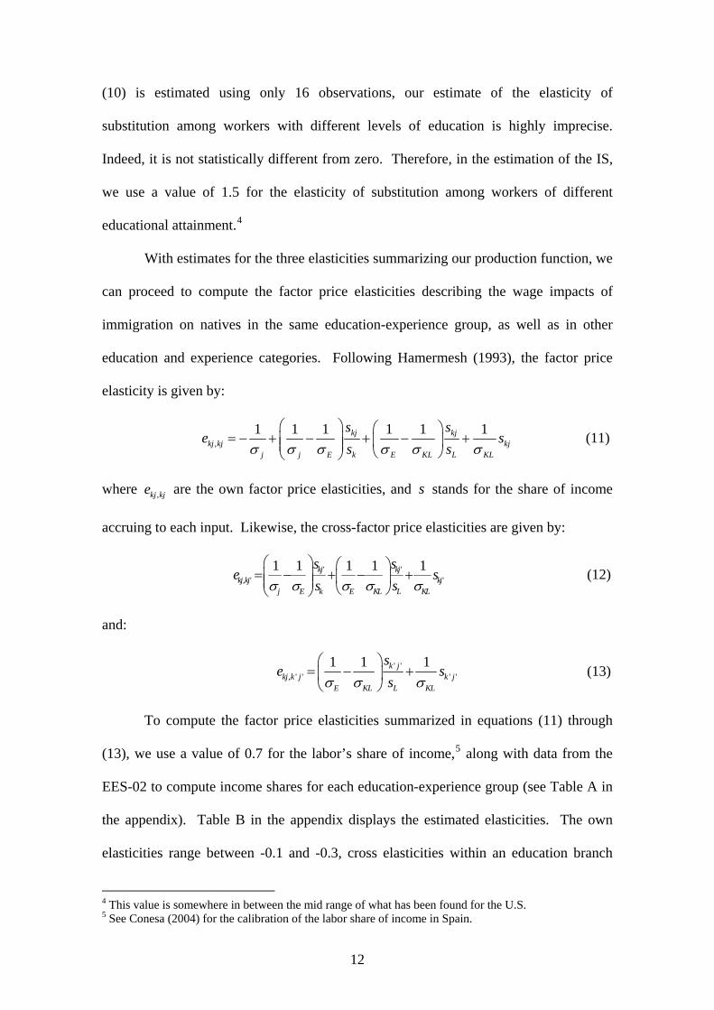
education and experience categories. Following Hamermesh (1993), the factor price
elasticity is given by:
,1 1 1 1 1 1kj kj
kj kj kjj j E k E KL L KL
s se s
s sσ σ σ σ σ σ⎛ ⎞ ⎛ ⎞
= − + − + − +⎜ ⎟ ⎜ ⎟⎜ ⎟ ⎝ ⎠⎝ ⎠ (11)
where are the own factor price elasticities, and stands for the share of income
accruing to each input. Likewise, the cross-factor price elasticities are given by:
,kj kje s
' ', ' '
1 1 1 1 1kj kjkj kj kj
j E k E KL L KL
s se s
s sσ σ σ σ σ⎛ ⎞ ⎛ ⎞
= − + − +⎜ ⎟ ⎜ ⎟⎜ ⎟ ⎝ ⎠⎝ ⎠ (12)
and:
' ', ' ' ' '
1 1 1k jkj k j k j
E KL L KL
se
sσ σ σ⎛ ⎞
= − +⎜ ⎟⎝ ⎠
s
(13)
To compute the factor price elasticities summarized in equations (11) through
(13), we use a value of 0.7 for the labor’s share of income,5 along with data from the
EES-02 to compute income shares for each education-experience group (see Table A in
the appendix). Table B in the appendix displays the estimated elasticities. The own
elasticities range between -0.1 and -0.3, cross elasticities within an education branch
4 This value is somewhere in between the mid range of what has been found for the U.S. 5 See Conesa (2004) for the calibration of the labor share of income in Spain.
12
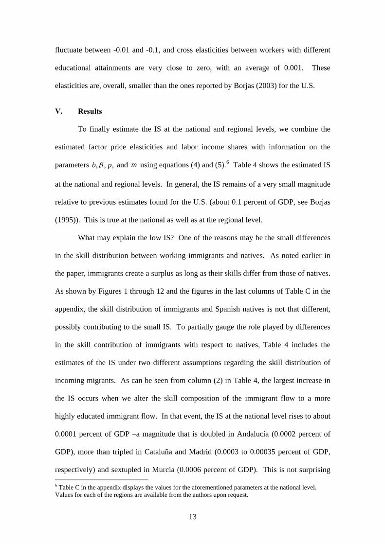
fluctuate between -0.01 and -0.1, and cross elasticities between workers with different
educational attainments are very close to zero, with an average of 0.001. These
elasticities are, overall, smaller than the ones reported by Borjas (2003) for the U.S.
V. Results
To finally estimate the IS at the national and regional levels, we combine the
estimated factor price elasticities and labor income shares with information on the
parameters ,,, pb β and using equations (4) and (5).m 6 Table 4 shows the estimated IS
at the national and regional levels. In general, the IS remains of a very small magnitude
relative to previous estimates found for the U.S. (about 0.1 percent of GDP, see Borjas
(1995)). This is true at the national as well as at the regional level.
What may explain the low IS? One of the reasons may be the small differences
in the skill distribution between working immigrants and natives. As noted earlier in
the paper, immigrants create a surplus as long as their skills differ from those of natives.
As shown by Figures 1 through 12 and the figures in the last columns of Table C in the
appendix, the skill distribution of immigrants and Spanish natives is not that different,
possibly contributing to the small IS. To partially gauge the role played by differences
in the skill contribution of immigrants with respect to natives, Table 4 includes the
estimates of the IS under two different assumptions regarding the skill distribution of
incoming migrants. As can be seen from column (2) in Table 4, the largest increase in
the IS occurs when we alter the skill composition of the immigrant flow to a more
highly educated immigrant flow. In that event, the IS at the national level rises to about
0.0001 percent of GDP –a magnitude that is doubled in Andalucía (0.0002 percent of
GDP), more than tripled in Cataluña and Madrid (0.0003 to 0.00035 percent of GDP,
respectively) and sextupled in Murcia (0.0006 percent of GDP). This is not surprising 6 Table C in the appendix displays the values for the aforementioned parameters at the national level. Values for each of the regions are available from the authors upon request.
13
given the greater share of income that accrues to more skilled workers and, in any event,
suggests that a potential explanation for the small size of the Spanish IS may lay on the
skill similarity between immigrants and natives.
Another reason for the low IS may reside in the lower factor price elasticities for
Spain relative to the U.S. (see Borjas (2003) for U.S. figures). We thus experiment with
imposing a much larger value for the factor price elasticity, i.e. -1. Indeed, we find that
the IS more than triples, rising from 2x10⁻⁶ percent of GDP in column (1) to 7x10⁻⁶
percent of GDP in column (4), Table 4. The numbers are, nevertheless, very small.
What may, nonetheless, explain the lower factor price elasticity in the Spanish case? Is
this a reasonable finding? We believe it is given the higher wage rigidity in Europe and,
in particular, Spain, relative to the U.S. The higher wage rigidity in Spain is a by-
product of a more regulated wage-setting that occurs through collective bargaining
agreements often negotiated at the sector and even national level.
In addition to the two aforementioned reasons, there are a number of
assumptions made in the model that could also play a role in the low IS. One example
is the assumption that iβ is exogenous. However, the parameter iβ is unlikely to be
exogenous as immigrants may locate themselves in regions where their skills are most
valued. Therefore, in column (5) of Table 4, we instrument this parameter with the
share of immigrants in a particular education-experience category at a national level.
The IS figures, however, become slightly smaller and, as such, do not suggest that the
endogeneity of iβ is causing an underestimate of the IS.
A third potential explanation for a small IS could be the size of the immigrant
shock, i.e. . The figures in columns (1) through (5) use the 2001 immigrant share in
the Spanish workforce. Because much of the increase in immigration has occurred in
recent years, we re-compute the IS using the 2006 figures. The figures in column (6)
m
14
indicate that the IS doubles from 2x10⁻⁶ percent of GDP in column (1) to 4x10⁻⁶ percent
of GDP in column (6). This is still a small figure. However, it is important to keep in
mind that, while immigrants account for up to 40 percent of the workforce in some U.S.
regions, in Spain this figure does not exceed 15 percent. A small immigrant shock may
not require a significant adjustment in factor prices, i.e. native wages, and,
consequently, may yield a low IS.
VI. Limitations of the Computed Immigration Surplus
At this juncture in the paper, it is worth discussing a couple of limitations in the
computation of the IS. A first limitation comes from the assumption of identical factor
price elasticities across the various Spanish regions. As noted by Ciccone and Peri
(2006), immigration may create positive externalities affecting the local wage structure.
In that event, we may underestimate factor price elasticities in those regions where the
externalities are larger. However, the assumption of factor price equalization across
regions in a smaller economy, like Spain, where wages are often negotiated at the sector
or national level in collective bargaining agreements is not far fetched. Furthermore,
while the computed IS under the assumption of a much larger factor price elasticity of
-1 (see column (4) in Table 4) increases in size, it does not remotely bring the IS
estimates close to the figures found for the U.S.
Yet, the most pressing limitation is the perfect substitutability between
immigrants and natives within a skill cell assumed by the three-level CES production
function. The latter suggests that immigrants and natives compete against each other
within each skill cell. A first way to assess whether this is the case is to compute the
index proposed by Altonji and Card (1991). As noted in Card (2001), the index for any
given occupation would be given by: q ∑= q qI
qN
qNI fffI /, , where and are
the fractions of natives and immigrants of a particular skill group employed in
Nqf I
qf
15

occupation , with reflecting the overall fraction of the workforce in that particular
cell employed in that occupation. If both immigrants and natives have similar
occupation distributions, the index should take value of 1, whereas immigrants and
natives with very distinct occupation distributions would result in an index close to zero.
Table 5 shows the index of competition for immigrants and natives computed using
occupations held by workers grouped at the one-digit ISCO-88 level so as to avoid some
empty occupation categories at the cell level. For all education-experience groups, we
find indexes with values near one; thus suggesting that immigrants and natives within a
skill group are likely to serve as fairly good substitutes.
q qf
However, the above index groups immigrants and natives at one-digit ISCO-88
occupational level categories, possibly not capturing any ongoing segregation within
skill level. Therefore, we use instead two-digit ISCO-88 occupational level categories
and plot the occupational distributions of immigrants and natives within a particular
skill level –defined by their educational attainment and age. If immigrants and natives
within skill groups are perfect substitutes, their occupational distributions within skill
levels should be very similar. For the sake of brevity, we display the plots of the
occupational distribution of immigrants and natives in the skill level where immigrant
density is at its highest, i.e. the skill level defined by having secondary level studies and
being younger than 30 years of age. Approximately 13.2 percent of immigrants in the
Spanish territory belong to this skill level, as well as 11.3 percent of immigrants in
Andalucía, 10.3 percent of immigrants in Cataluña, 15 percent of immigrants in
Valencia, 14.4 percent of immigrants in Madrid and 17.1 percent of immigrants in
Murcia. One of the facts revealed by Figures 13 through 18 is the unequal occupational
distribution of immigrants and natives within the skill level under consideration.
Immigrants younger than 30 years of age with secondary studies are more frequently
16

working in jobs for non-qualified workers in the 91 through 99 occupational coding
range relative to similarly skilled natives. This finding is suggestive of their imperfect
substitutability within a skill cell. Therefore, the assumption of perfect substitutability
between immigrants and natives within a skill cell may not be a reasonable one once we
consider a fine occupational disaggregated level.
VII. Summary and Conclusions
Spain has experienced growing immigration inflows during the past decade. As
such, it is only logical to question how these new immigrants have affected Spanish
natives. Additionally, given the uneven distribution of immigrants throughout the
Spanish territory and the important labor market disequilibria found across Spanish
regions, it is also important to understand how the recent immigrant inflows’ impact
may have differed across Spanish regions. In this paper, we address these questions
using data from the 2001 Census, along with aggregate time series data from the 1995
and 2002 Current Population Surveys and Earnings Structure Surveys. With the
aforementioned data, and assuming a three-level CES production function along with
minimal interregional labor mobility or shifts in the production of goods that intensively
employ migrants (Lewis 2003), we compute the immigration surplus (IS) accruing to
Spanish natives at the national and regional levels via changes in relative factor prices.
We find a small IS of approximately 2x10⁻⁶ percent of GDP, which increases to 0.0001
percent of GDP depending on the assumptions made in the calculation. The IS accruing
to the regions receiving most immigrants is up to six times larger, i.e. Murcia. Yet,
these figures still remain well below previous estimates for the U.S. (about 0.1 percent
of GDP, see Borjas (1995)).
After reviewing the various model assumptions possibly driving our results, we
conclude that there are two potential reasons for the small value of the IS in Spain:
17
(1) the small differences in the skill distribution of immigrants and Spanish natives, and
(2) the relatively low factor price elasticity characteristic of countries with greater wage
rigidities, such as Spain. High wage rigidity is often due to the broad collective
bargaining agreements typically used as the principal wage-setting mechanism.
Additionally, we note that the computed IS assumes perfect substitutability
within cells between immigrants and natives. Yet, the two-digit level occupational
distribution of natives and immigrants within the skill group with the largest
concentration of immigrants (i.e. the skill group corresponding to a secondary education
and 30 years of age or younger) is far from similar. Instead, immigrants seem to be
more concentrated in non-qualified occupations in the 91 through 99 coding range than
their similarly skilled native counterparts, challenging the validity of the assumption of
perfect substitutability of immigrants and natives within a skill level and, as such, the IS
being computed.
Finally, it is worth noting that the computed IS does not take into account the
fact that immigrants create consumption externalities. Specifically, increase the demand
for various goods and services. The growing demand shifts the labor demand curve to
the right, creates employment, and raises the IS beyond the figure computed herein.
Likewise, the IS does not include other costs and benefits from immigration. As such, a
low IS does not imply that immigrants do not significantly impact the Spanish economy.
We know they do in a variety of facets. For instance, immigrants alter the demand for
social and educational services, typically financed through income taxes. Similarly, the
IS ignores the contribution of immigrants to the population pyramid –a contribution that
may be crucial in financing the retirement of a progressively older population owing to
declining fertility rates and increasing longevity.
18

References
Altonji, Joseph and D. Card (2001), “The effect of immigration on the labor market
outcomes of less-skilled natives” in John M. Abowd and Richard Freeman, eds,
Immigration, Trade and the Labor Market. Chicago: The University of Chicago Press,
1991.
Bentolila, Samuel (2001), “Las Migraciones Interiores in España”, Working Paper
FEDEA # 2001-07.
Borjas, George (1995), “The Economic Benefits of Immigration”, Journal of Economic
Perspectives, vol. 9, nº. 2.
Borjas, George (2003), “The Labor Demand Curve is Downward Sloping: Reexamining
the impacts of Immigration on the Labor Market” Quarterly Journal of Economics, 118,
pages: 1334-1374.
Card, David (2001), “Immigrant Inflows, Native Outflows and the Local Labor Market
Impacts of Higher Immigration” Journal of Labor Economics, 19 (January).
Card David and Thomas Lemieux (2001), “Can Falling Supply explain the rising
returns to College for Younger Men? A Cohort Based Analysis” Quarterly Journal of
Economics, Vol. CXVI, pages: 705-746.
Ciccone, Antonio and Giovanni Peri (2006), “Identifying Human-Capital Externalities:
Theory and Evidence” Review of Economic Studies, 73, pages: 381-412.
Conesa, Juan and Timothy Kehoe (2004), “Productivity, Taxes and Hours worked in
Spain: 1970-2000” mimeo.
19

Hamermesh Daniel (1993), “Labor Demand”, Princeton University Press, Princeton
New Jersey, 1993.
Katz, Larry and Murphy, Kevin (1992), “Change in Relative Wages 1963-1987: Supply
and Demand Factors” Quarterly Journal of Economics 107, pages 35-38.
Lewis, Ethan (2003), “Local Open Economies within the US: How do industries
respond to Immigration?” Working Paper No. 04-1, Federal Reserve Bank of
Philadelphia.
Ottaviano, Gianmarco and G. Peri (2005), “Rethinking the Gains from Immigration:
Theory and Evidence from the US” NBER Working Paper # 11672.
Ottaviano, Gianmarco and G. Peri (2006), “Rethinking the Gains from Immigration on
Wages” NBER Working Paper # 12497
Peri, Giovanni (2006), “Immigrants' Complementarities and Native Wages: Evidence
from California”, Working Paper, University of California.
20

Table 1: Percentage of Immigrants in Population and Employment (1991-2005)
Percent of Immigrants in the Adult Population
Percent of Immigrants in the Adult Employed Population Regions 1991
Census 2001
Census 2005
Padrón 1991
Census 2001
Census 2005
Padrón
Average 1.2 4.0 8.5 1.1 4.6 10.9 Andalucía 1.0 2.5 5.6 0.8 2.9 7.2 Aragón 0.5 3.0 7.2 0.5 4.1 10.0 Asturias 0.8 1.3 2.7 0.7 1.6 3.1 Balearic Islands 2.9 8.4 16.3 2.3 8.4 18.9 Canary I. 2.6 6.1 11.5 0.3 6.2 14.0 Cantabria 0.7 1.3 3.8 0.4 1.5 4.9 C. León 0.5 1.5 3.5 0.5 1.9 5.0 C. La Mancha 0.2 2.9 6.1 0.2 3.4 8.6 Cataluña 1.6 4.6 11.3 1.4 5.2 12.9 C. Valenciana 1.6 5.6 12.6 0.8 5.3 15.4 Extremadura 0.3 1.2 1.9 0.3 1.5 2.4 Galicia 1.1 1.2 2.6 0.9 1.3 2.9 Madrid 1.9 6.6 13.2 1.7 8.4 17.0 Murcia 0.4 5.9 12.5 0.4 8.8 16.3 Navarra 0.6 4.1 7.8 0.6 5.1 10.0 P.Vasco 0.6 1.5 3.5 0.5 1.6 4.5 Rioja 0.6 4.5 10.4 0.7 5.5 13.1 C. y Melilla 0.3 7.8 - 2.7 5.4 -
Note: The adult population is defined as individuals 16 years of age and older. Adult Population (1991 Census): 30,665,000. Adult Population (2001 Census): 34,223,000. Adult Population (2005 Padrón): 36,415,975.
21
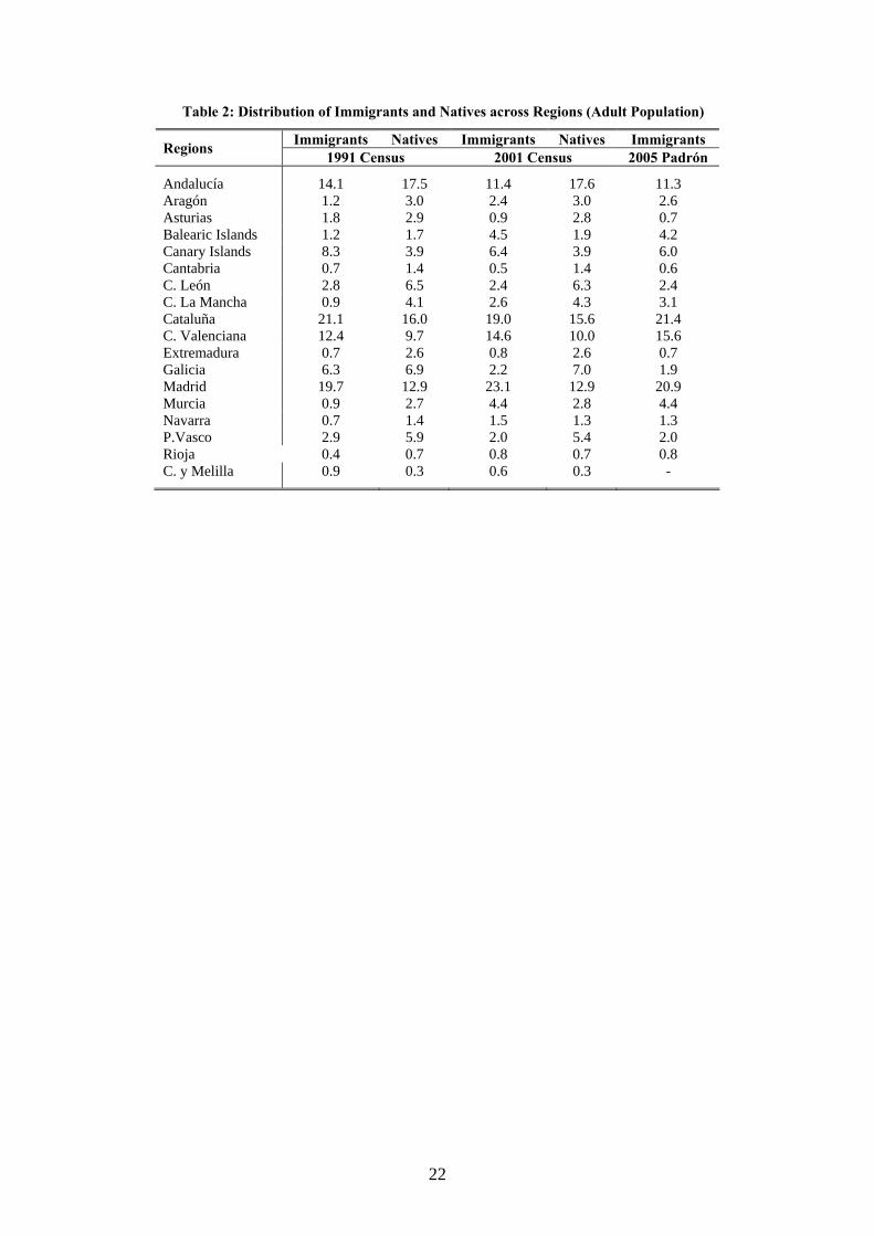
Table 2: Distribution of Immigrants and Natives across Regions (Adult Population)
Immigrants Natives Immigrants Natives Immigrants Regions 1991 Census 2001 Census 2005 Padrón
Andalucía 14.1 17.5 11.4 17.6 11.3 Aragón 1.2 3.0 2.4 3.0 2.6 Asturias 1.8 2.9 0.9 2.8 0.7 Balearic Islands 1.2 1.7 4.5 1.9 4.2 Canary Islands 8.3 3.9 6.4 3.9 6.0 Cantabria 0.7 1.4 0.5 1.4 0.6 C. León 2.8 6.5 2.4 6.3 2.4 C. La Mancha 0.9 4.1 2.6 4.3 3.1 Cataluña 21.1 16.0 19.0 15.6 21.4 C. Valenciana 12.4 9.7 14.6 10.0 15.6 Extremadura 0.7 2.6 0.8 2.6 0.7 Galicia 6.3 6.9 2.2 7.0 1.9 Madrid 19.7 12.9 23.1 12.9 20.9 Murcia 0.9 2.7 4.4 2.8 4.4 Navarra 0.7 1.4 1.5 1.3 1.3 P.Vasco 2.9 5.9 2.0 5.4 2.0 Rioja 0.4 0.7 0.8 0.7 0.8 C. y Melilla 0.9 0.3 0.6 0.3 -
22

Table 3: Elasticities of Substitution at the National Level (Dependent Variable: Log Gross Annual Earnings)
Elasticity of Substitution across Experience Groups (1/ jσ )
Elasticity of Substitution across Educational Groups (1/ Eσ )
OLS IV OLS IV
-0.057
(0.014)
-0.19
(0.07)
-0.139
(0.08)
-0.08
(0.08)
Note: The regressions estimating (1/ jσ ) include 7 education fixed-effects, 6 fixed-age effects, 1 year effect, interactions between year and education effects and interactions between year and age effects. We do not include interaction terms between education and experience (age) groups because the total number of observations in those regressions is only 112. We instrument the log of the number employed in each cell with the number of working immigrants in that cell at the national level. The regressions estimating (1/ Eσ ) include 1 year effect and interactions between education and year effects. The number of observations in those regressions is only 16 and the same instruments used in the estimation of (1/ jσ ) is used.
23
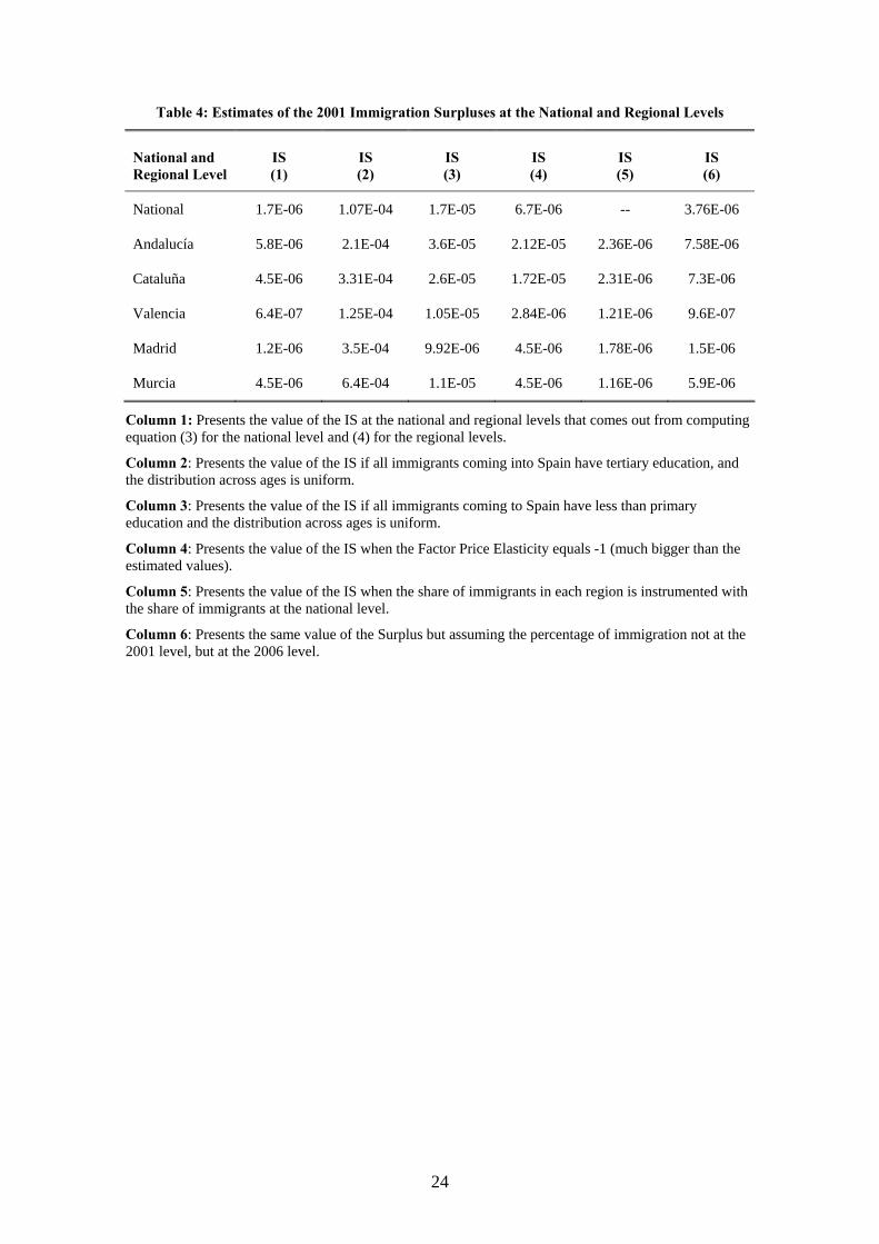
Table 4: Estimates of the 2001 Immigration Surpluses at the National and Regional Levels
National and Regional Level
IS (1)
IS (2)
IS (3)
IS (4)
IS (5)
IS (6)
National 1.7E-06 1.07E-04 1.7E-05 6.7E-06 -- 3.76E-06
Andalucía 5.8E-06 2.1E-04 3.6E-05 2.12E-05 2.36E-06 7.58E-06
Cataluña 4.5E-06 3.31E-04 2.6E-05 1.72E-05 2.31E-06 7.3E-06
Valencia 6.4E-07 1.25E-04 1.05E-05 2.84E-06 1.21E-06 9.6E-07
Madrid 1.2E-06 3.5E-04 9.92E-06 4.5E-06 1.78E-06 1.5E-06
Murcia 4.5E-06 6.4E-04 1.1E-05 4.5E-06 1.16E-06 5.9E-06
Column 1: Presents the value of the IS at the national and regional levels that comes out from computing equation (3) for the national level and (4) for the regional levels.
Column 2: Presents the value of the IS if all immigrants coming into Spain have tertiary education, and the distribution across ages is uniform.
Column 3: Presents the value of the IS if all immigrants coming to Spain have less than primary education and the distribution across ages is uniform.
Column 4: Presents the value of the IS when the Factor Price Elasticity equals -1 (much bigger than the estimated values).
Column 5: Presents the value of the IS when the share of immigrants in each region is instrumented with the share of immigrants at the national level.
Column 6: Presents the same value of the Surplus but assuming the percentage of immigration not at the 2001 level, but at the 2006 level.
24

Table 5: Occupational Distribution of Natives and Immigrants, by Skill Group
Education Age Index of Competition
Less than Primary <30 0.952 Less than Primary 30-34 0.957 Less than Primary 35-39 0.967 Less than Primary 40-44 0.970 Less than Primary 45-49 0.986 Less than Primary 50-54 0.995 Less than Primary >54 0.996 Primary <30 0.984 Primary 30-34 0.973 Primary 35-39 0.979 Primary 40-44 0.984 Primary 45-49 0.988 Primary 50-54 0.995 Primary >54 0.997 Secondary <30 0.986 Secondary 30-34 0.980 Secondary 35-39 0.982 Secondary 40-44 0.984 Secondary 45-49 0.988 Secondary 50-54 0.993 Secondary >54 0.995 Vocational Training (1st cycle) <30 0.992 Vocational Training (1st cycle) 30-34 0.989 Vocational Training (1st cycle) 35-39 0.993 Vocational Training (1st cycle) 40-44 0.978 Vocational Training (1st cycle) 45-49 0.992 Vocational Training (1st cycle) 50-54 0.997 Vocational Training(1st cycle) >54 0.995 Vocational Training (2nd cycle) <30 0.993 Vocational Training (2nd cycle) 30-34 0.983 Vocational Training (2nd cycle) 35-39 0.984 Vocational Training (2nd cycle) 40-44 0.970 Vocational Training (2nd cycle) 45-49 0.976 Vocational Training (2nd cycle) 50-54 0.989 Vocational Training (2nd cycle) >54 0.994 High School <30 0.943 High School 30-34 0.912 High School 35-39 0.938 High School 40-44 0.949 High School 45-49 0.947 High School 50-54 0.972 High School >54 0.992 University (1st cycle) <30 0.975 University (1st cycle) 30-34 0.949 University (1st cycle) 35-39 0.943 University (1st cycle) 40-44 0.957 University (1st cycle) 45-49 0.965 University (1st cycle) 50-54 0.986 University (1st cycle) >54 0.994 University (2nd cycle) <30 0.976 University (2nd cycle) 30-34 0.963 University (2nd cycle) 35-39 0.942 University (2nd cycle) 40-44 0.960 University (2nd cycle) 45-49 0.966 University (2nd cycle) 50-54 0.993 University (2nd cycle) >54 0.993
25
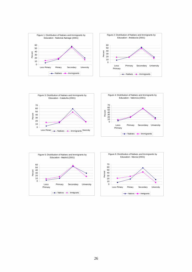
Figure 1: Distribution of Natives and Immigrants by Education - National Average (2001)
0102030405060
Less Primary Primary Secondary University
Perc
ent
Natives Immigrants
Figure 2: Distribution of Natives and Immigrants by Education - Andalucía (2001)
0102030405060
LessPrimary
Primary Secondary University
Perc
ent
Natives Immigrants
Figure 3: Distribution of Natives and Immigrants by Education - Cataluña (2001)
010203040506070
Less Primary Primary Secondary University
Perc
ent
Natives Immigrants
Figure 4: Distribution of Natives and Immigrants by Education - Valencia (2001)
010203040506070
LessPrimary
Primary Secondary University
Perc
ent
Natives Immigrants
Figure 5: Distribution of Natives and Immigrants by Education - Madrid (2001)
0102030405060
LessPrimary
Primary Secondary University
Perc
ent
Natives Immigrants
Figure 6: Distribution of Natives and Immigrants by Education - Murcia (2001)
010203040506070
Less Primary Primary Secondary University
Perc
ent
Natives Immigrants
26

Figure 7: Age Distribution of Native and Immigrant Workers - National Average (2001)
05
1015202530354045
16-24 25-34 35-44 45-65
Perc
enta
ge
Natives Immigrants
Figure 8: Age Distribution of Native and Immigrant Workers Andalucía (2001)
05
10152025303540
16-24 25-34 35-44 45-65
Perc
enta
ge
Natives Immigrants
Figure 9: Age Distribution of Native and Immigrant Workers Catalonia (2001)
05
1015202530354045
16-24 25-34 35-44 45-65
Perc
enta
ge
Natives Immigrants
Figure 10: Age Distribution of Native and Immigrant Workers Valencia (2001)
05
1015202530354045
16-24 25-34 35-44 45-65
Perc
enta
ge
Natives Immigrants
Figure 11: Age Distribution of Native and Immigrant Workers Madrid (2001)
05
1015202530354045
16-24 25-34 35-44 45-65
Perc
enta
ge
Natives Immigrants
Figure 12: Age Distribution of Native and Immigrant Workers Murcia (2001)
0
10
20
30
40
50
16-24 25-34 35-44 45-65
Perc
enta
ge
Natives Immigrants
27
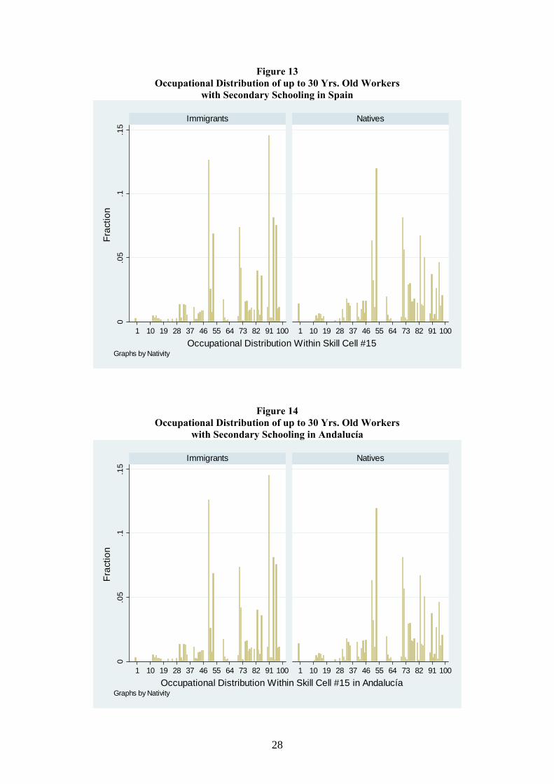
Figure 13 Occupational Distribution of up to 30 Yrs. Old Workers
with Secondary Schooling in Spain
0.0
5.1
.15
1 10 19 28 37 46 55 64 73 82 91 100 1 10 19 28 37 46 55 64 73 82 91 100
Immigrants NativesFr
actio
n
Occupational Distribution Within Skill Cell #15Graphs by Nativity
Figure 14 Occupational Distribution of up to 30 Yrs. Old Workers
with Secondary Schooling in Andalucía
0.0
5.1
.15
1 10 19 28 37 46 55 64 73 82 91 100 1 10 19 28 37 46 55 64 73 82 91 100
Immigrants Natives
Frac
tion
Occupational Distribution Within Skill Cell #15 in AndalucíaGraphs by Nativity
28
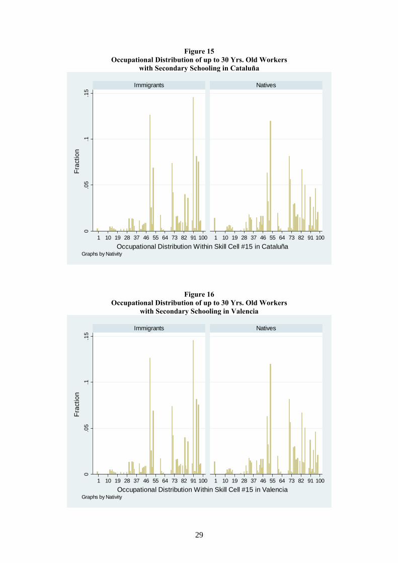
Figure 15 Occupational Distribution of up to 30 Yrs. Old Workers
with Secondary Schooling in Cataluña
0.0
5.1
.15
1 10 19 28 37 46 55 64 73 82 91 100 1 10 19 28 37 46 55 64 73 82 91 100
Immigrants NativesFr
actio
n
Occupational Distribution Within Skill Cell #15 in CataluñaGraphs by Nativity
Figure 16 Occupational Distribution of up to 30 Yrs. Old Workers
with Secondary Schooling in Valencia
0.0
5.1
.15
1 10 19 28 37 46 55 64 73 82 91 100 1 10 19 28 37 46 55 64 73 82 91 100
Immigrants Natives
Frac
tion
Occupational Distribution Within Skill Cell #15 in ValenciaGraphs by Nativity
29
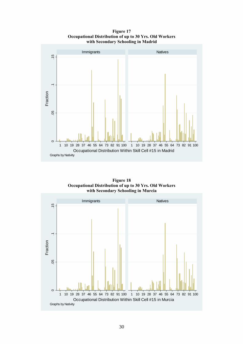
Figure 17 Occupational Distribution of up to 30 Yrs. Old Workers
with Secondary Schooling in Madrid
0.0
5.1
.15
1 10 19 28 37 46 55 64 73 82 91 100 1 10 19 28 37 46 55 64 73 82 91 100
Immigrants NativesFr
actio
n
Occupational Distribution Within Skill Cell #15 in MadridGraphs by Nativity
Figure 18 Occupational Distribution of up to 30 Yrs. Old Workers
with Secondary Schooling in Murcia
0.0
5.1
.15
1 10 19 28 37 46 55 64 73 82 91 100 1 10 19 28 37 46 55 64 73 82 91 100
Immigrants Natives
Frac
tion
Occupational Distribution Within Skill Cell #15 in MurciaGraphs by Nativity
30

APPENDIX TABLES Table A: Income Shares, by Skill Group
Education Age Cell Income
Shares
Income Shares (within education
branch)
Less than Primary <30 0.001 0.018 Less than Primary 30-34 0.001 0.018 Less than Primary 35-39 0.001 0.018 Less than Primary 40-44 0.002 0.018 Less than Primary 45-49 0.003 0.018 Less than Primary 50-54 0.005 0.018 Less than Primary >54 0.007 0.018 Primary <30 0.012 0.132 Primary 30-34 0.007 0.132 Primary 35-39 0.010 0.132 Primary 40-44 0.021 0.132 Primary 45-49 0.029 0.132 Primary 50-54 0.031 0.132 Primary >54 0.036 0.132 Secondary <30 0.063 0.132 Secondary 30-34 0.029 0.205 Secondary 35-39 0.033 0.205 Secondary 40-44 0.028 0.205 Secondary 45-49 0.020 0.205 Secondary 50-54 0.016 0.205 Secondary >54 0.012 0.205 Vocational Training (1st cycle) <30 0.016 0.052 Vocational Training (1st cycle) 30-34 0.008 0.052 Vocational Training (1st cycle) 35-39 0.010 0.052 Vocational Training (1st cycle) 40-44 0.006 0.052 Vocational Training (1st cycle) 45-49 0.005 0.052 Vocational Training (1st cycle) 50-54 0.003 0.052 Vocational Training(1st cycle) >54 0.002 0.052 Vocational Training (2nd cycle) <30 0.025 0.074 Vocational Training (2nd cycle) 30-34 0.012 0.106 Vocational Training (2nd cycle) 35-39 0.010 0.106 Vocational Training (2nd cycle) 40-44 0.008 0.106 Vocational Training (2nd cycle) 45-49 0.007 0.106 Vocational Training (2nd cycle) 50-54 0.005 0.106 Vocational Training (2nd cycle) >54 0.004 0.106 High School <30 0.026 0.100 High School 30-34 0.012 0.100 High School 35-39 0.014 0.100 High School 40-44 0.015 0.100 High School 45-49 0.014 0.100 High School 50-54 0.008 0.100 High School >54 0.006 0.100 University (1st cycle) <30 0.014 0.056 University (1st cycle) 30-34 0.008 0.080 University (1st cycle) 35-39 0.008 0.080 University (1st cycle) 40-44 0.007 0.080 University (1st cycle) 45-49 0.007 0.080 University (1st cycle) 50-54 0.006 0.080 University (1st cycle) >54 0.006 0.080 University (2nd cycle) <30 0.013 0.063 University (2nd cycle) 30-34 0.010 0.063 University (2nd cycle) 35-39 0.011 0.063 University (2nd cycle) 40-44 0.008 0.063 University (2nd cycle) 45-49 0.008 0.063 University (2nd cycle) 50-54 0.005 0.063 University (2nd cycle) >54 0.006 0.063
31
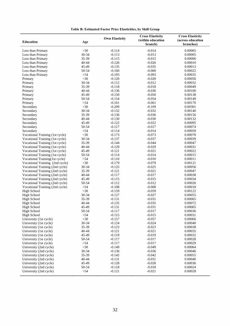
Table B: Estimated Factor Price Elasticities, by Skill Group
Education Age Own Elasticity
Cross Elasticity (within education
branch)
Cross Elasticity (across education
branches)
Less than Primary <30 -0.114 -0.014 0.00005 Less than Primary 30-34 -0.113 -0.013 0.00005 Less than Primary 35-39 -0.115 -0.015 0.00006 Less than Primary 40-44 -0.126 -0.026 0.00010 Less than Primary 45-49 -0.135 -0.035 0.00013 Less than Primary 50-54 -0.160 -0.060 0.00022 Less than Primary >54 -0.193 -0.093 0.00035 Primary <30 -0.120 -0.020 0.00056 Primary 30-34 -0.112 -0.012 0.00032 Primary 35-39 -0.118 -0.018 0.00049 Primary 40-44 -0.136 -0.036 0.00100 Primary 45-49 -0.150 -0.050 0.00138 Primary 50-54 -0.154 -0.054 0.00149 Primary >54 -0.161 -0.061 0.00170 Secondary <30 -0.209 -0.109 0.00301 Secondary 30-34 -0.132 -0.032 0.00140 Secondary 35-39 -0.136 -0.036 0.00156 Secondary 40-44 -0.130 -0.030 0.00132 Secondary 45-49 -0.122 -0.022 0.00095 Secondary 50-54 -0.117 -0.017 0.00074 Secondary >54 -0.114 -0.014 0.00059 Vocational Training (1st cycle) <30 -0.173 -0.073 0.00078 Vocational Training (1st cycle) 30-34 -0.137 -0.037 0.00039 Vocational Training (1st cycle) 35-39 -0.144 -0.044 0.00047 Vocational Training (1st cycle) 40-44 -0.129 -0.029 0.00031 Vocational Training (1st cycle) 45-49 -0.121 -0.021 0.00022 Vocational Training (1st cycle) 50-54 -0.114 -0.014 0.00015 Vocational Training(1st cycle) >54 -0.110 -0.010 0.00011 Vocational Training (2nd cycle) <30 -0.179 -0.079 0.00121 Vocational Training (2nd cycle) 30-34 -0.125 -0.025 0.00056 Vocational Training (2nd cycle) 35-39 -0.121 -0.021 0.00047 Vocational Training (2nd cycle) 40-44 -0.117 -0.017 0.00038 Vocational Training (2nd cycle) 45-49 -0.115 -0.015 0.00034 Vocational Training (2nd cycle) 50-54 -0.112 -0.012 0.00026 Vocational Training (2nd cycle) >54 -0.108 -0.008 0.00018 High School <30 -0.159 -0.059 0.00122 High School 30-34 -0.127 -0.027 0.00055 High School 35-39 -0.131 -0.031 0.00065 High School 40-44 -0.135 -0.035 0.00072 High School 45-49 -0.131 -0.031 0.00065 High School 50-54 -0.117 -0.017 0.00036 High School >54 -0.115 -0.015 0.00031 University (1st cycle) <30 -0.157 -0.057 0.00066 University (1st cycle) 30-34 -0.124 -0.024 0.00040 University (1st cycle) 35-39 -0.123 -0.023 0.00038 University (1st cycle) 40-44 -0.121 -0.021 0.00035 University (1st cycle) 45-49 -0.119 -0.019 0.00032 University (1st cycle) 50-54 -0.117 -0.017 0.00028 University (1st cycle) >54 -0.117 -0.017 0.00029 University (2nd cycle) <30 -0.149 -0.049 0.00064 University (2nd cycle) 30-34 -0.136 -0.036 0.00046 University (2nd cycle) 35-39 -0.142 -0.042 0.00055 University (2nd cycle) 40-44 -0.131 -0.031 0.00040 University (2nd cycle) 45-49 -0.128 -0.028 0.00036 University (2nd cycle) 50-54 -0.118 -0.018 0.00024 University (2nd cycle) >54 -0.121 -0.021 0.00028
32

Table C: Parameter Estimates, by Skill Group
Education Age p m β b
Less than Primary <30 0.007 0.047 0.048 0.005 Less than Primary 30-34 0.004 0.047 0.023 0.003 Less than Primary 35-39 0.004 0.047 0.019 0.004 Less than Primary 40-44 0.006 0.047 0.016 0.006 Less than Primary 45-49 0.007 0.047 0.009 0.007 Less than Primary 50-54 0.009 0.047 0.004 0.010 Less than Primary >54 0.015 0.047 0.003 0.015 Primary <30 0.036 0.047 0.081 0.034 Primary 30-34 0.018 0.047 0.035 0.017 Primary 35-39 0.021 0.047 0.028 0.020 Primary 40-44 0.023 0.047 0.020 0.023 Primary 45-49 0.024 0.047 0.013 0.024 Primary 50-54 0.023 0.047 0.007 0.024 Primary >54 0.026 0.047 0.005 0.027 Secondary <30 0.105 0.047 0.132 0.104 Secondary 30-34 0.044 0.047 0.049 0.044 Secondary 35-39 0.043 0.047 0.037 0.044 Secondary 40-44 0.039 0.047 0.025 0.040 Secondary 45-49 0.032 0.047 0.017 0.033 Secondary 50-54 0.025 0.047 0.009 0.025 Secondary >54 0.019 0.047 0.007 0.020 Vocational Training (1st cycle) <30 0.026 0.047 0.019 0.026 Vocational Training (1st cycle) 30-34 0.011 0.047 0.008 0.012 Vocational Training (1st cycle) 35-39 0.010 0.047 0.005 0.010 Vocational Training (1st cycle) 40-44 0.006 0.047 0.004 0.006 Vocational Training (1st cycle) 45-49 0.004 0.047 0.002 0.004 Vocational Training (1st cycle) 50-54 0.003 0.047 0.002 0.003 Vocational Training(1st cycle) >54 0.002 0.047 0.001 0.002 Vocational Training (2nd cycle) <30 0.033 0.047 0.017 0.034 Vocational Training (2nd cycle) 30-34 0.015 0.047 0.009 0.015 Vocational Training (2nd cycle) 35-39 0.011 0.047 0.007 0.011 Vocational Training (2nd cycle) 40-44 0.006 0.047 0.004 0.006 Vocational Training (2nd cycle) 45-49 0.004 0.047 0.003 0.004 Vocational Training (2nd cycle) 50-54 0.003 0.047 0.002 0.003 Vocational Training (2nd cycle) >54 0.002 0.047 0.001 0.002 High School <30 0.042 0.047 0.075 0.040 High School 30-34 0.021 0.047 0.037 0.020 High School 35-39 0.021 0.047 0.028 0.020 High School 40-44 0.018 0.047 0.018 0.019 High School 45-49 0.012 0.047 0.011 0.013 High School 50-54 0.007 0.047 0.006 0.007 High School >54 0.005 0.047 0.005 0.005 University (1st cycle) <30 0.031 0.047 0.020 0.031 University (1st cycle) 30-34 0.016 0.047 0.014 0.016 University (1st cycle) 35-39 0.014 0.047 0.011 0.014 University (1st cycle) 40-44 0.013 0.047 0.007 0.013 University (1st cycle) 45-49 0.009 0.047 0.004 0.009 University (1st cycle) 50-54 0.007 0.047 0.003 0.007 University (1st cycle) >54 0.006 0.047 0.002 0.006 University (2nd cycle) <30 0.030 0.047 0.024 0.031 University (2nd cycle) 30-34 0.022 0.047 0.021 0.022 University (2nd cycle) 35-39 0.019 0.047 0.017 0.019 University (2nd cycle) 40-44 0.016 0.047 0.012 0.016 University (2nd cycle) 45-49 0.011 0.047 0.007 0.011 University (2nd cycle) 50-54 0.007 0.047 0.005 0.007 University (2nd cycle) >54 0.006 0.047 0.004 0.006
33